3D hydrodynamic simulations of massive main-sequence stars. I. Dynamics and mixing of convection and internal gravity waves

Abstract

We performed 3D hydrodynamic simulations of the inner $\approx 50\%$ radial extent of a $25\;\mathrm{\mathrm{M}_{\odot}}$ star in the early phase of the main sequence and investigate core convection and internal gravity waves in the core-envelope boundary region. Simulations for different grid resolutions and driving luminosities establish scaling relations to constrain models of mixing for 1D applications. As in previous works, the turbulent mass entrainment rate extrapolated to nominal heating is unrealistically high ($1.58\times 10^{-4}\;\mathrm{\mathrm{M}_{\odot}\,{\mathrm{yr}}^{-1}}$), which is discussed in terms of the non-equilibrium response of the simulations to the initial stratification. We measure quantitatively the effect of mixing due to internal gravity waves excited by core convection interacting with the boundary in our simulations. The wave power spectral density as a function of frequency and wavelength agrees well with the GYRE eigenmode predictions based on the 1D spherically averaged radial profile. A diffusion coefficient profile that reproduces the spherically averaged abundance distribution evolution is determined for each simulation. Through a combination of eigenmode analysis and scaling relations it is shown that in the $N^{2}$-peak region, mixing is due to internal gravity waves and follows the scaling relation $D_{\mathrm{IGW-hydro}}\propto L^{4/3}$ over a $\goa 2\;\mathrm{\mathrm{dex}}$ range of heating factors. Different extrapolations of the mixing efficiency down to nominal heating are discussed. If internal gravity wave mixing is due to thermally-enhanced shear mixing, an upper limit is $D_{\mathrm{IGW}}\loa 2$ to $3\times 10^{4}\;\mathrm{cm^{2}/s}$ at nominal heating in the $N^{2}$-peak region above the convective core.

1 Introduction

The properties of core convection determine the observational properties of main-sequence stars individually and as a population and set the stage for all subsequent evolutionary phases of intermediate mass and massive stars. Convective boundary mixing (CBM) infuences the main-sequence lifetime and the internal stratification for later evolutionary phases. It has been calibrated in 1D stellar evolution models by comparing model predictions with the observed width of the main sequence either from photometry or spectroscopy (e.g. Schaller et al., 1992; Kozhurina-Platais et al., 1997) or from eclipsing binaries (e.g. Stancliffe et al., 2015; Claret & Torres, 2019; Tkachenko et al., 2020). It is now also possible to constrain CBM through asteroseismology observations (e.g. Moravveji et al., 2015; Noll et al., 2021), and even more detailed model properties such as the temperature gradient or mixing in the stable layer may be constrained in the future (Pedersen et al., 2018; Michielsen et al., 2019; Michielsen et al., 2021; Bowman & Michielsen, 2021). For massive stars, the observed width of the main sequence appears to require more efficient mixing beyond the convective core compared to the range of values typically calibrated with the methods mentioned above (Castro et al., 2014; Schneider et al., 2018).

Observations of massive main-sequence stars also show clear observational evidence of mixing in the stable layers all the way to the surface. Venn et al. (2002) reported depletion of B and simultaneous enrichment of N in B-type stars that generally matched the predictions of rotating stars. However, more recent work has revealed a picture that appears to be more complicated, such as larger N enhancement and B depletion than predicted by rotating models (Mendel et al., 2006; Martins et al., 2015) and slowly rotating N-enriched stars (Morel et al., 2008; Hunter et al., 2008; Dufton et al., 2018) in which rotation-induced mixing predictions seem to fall short and additional physics processes must be at work. In a careful statistical analysis, Aerts et al. (2014) found that observed stellar rotation rates have no predictive power regarding the observed N enhancement (see also Markova et al., 2018). This adds to the motivation to investigate and possibly identify and quantify mixing processes that are unrelated to rotation in the stable layers of massive stars.

One such possible transport mechanism is internal gravity waves (IGW) (Press, 1981; Talon & Charbonnel, 2005) that would transport species (Garcia Lopez & Spruit, 1991; Denissenkov & Tout, 2003) and angular momentum (Kumar et al., 1999). Analytical approaches such as those mentioned rely on a number of assumptions, such as the wave-generating mechanism and power spectrum as well as the fundamental transport physics of IGWs (Lecoanet & Quataert, 2013). Ultimately, realistic representations of these complicated fluid-dynamics properties can be revealed by multi-dimensional hydrodynamic simulations. IGWs have indeed been observed and analyzed in numerous simulations, for example of solar-type stars (Dintrans et al., 2005; Rogers et al., 2006; Alvan et al., 2015), of He-shell flash convection (Herwig et al., 2006), and of O-shell and core convection (Meakin & Arnett, 2007; Gilet et al., 2013; Browning et al., 2004). Based on 2D simulations, Rogers et al. (2013) investigated the role of IGWs in transporting angular momentum in massive stars. Predicting (Aerts & Rogers, 2015) and indeed observing (Bowman et al., 2019a, b, 2020) oscillations due to stochastically excited IGWs in massive stars has triggered renewed efforts to determine the quantitative properties of IGW spectra from 2D (Horst et al., 2020) and 3D (Edelmann et al., 2019) simulations.

Despite great progress in multi-dimensional convection simulations in general and of core convection in massive stars specifically, the computational cost of these simulations is still placing severe limitations on obtaining quantitative and even qualitative results. Attempts to determine quantitative mixing efficiencies of IGWs from simulations are still in their infancy. As far as we are aware, only Rogers & McElwaine (2017) derived a diffusion coefficient profile for IGW mixing for the radiative envelope from anelastic 2D simulations of a $3\mathrm{M}_{\odot}$ star based on a tracer-particle post-processing approach (similar to the approach by Freytag et al., 1996; Herwig et al., 2006). However, the actual magnitude could not be reliably determined. When applied in 1D stellar evolution calculations, the diffusion coefficients from the 2D simulations had to be reduced by approximately four orders of magnitude in order to match asteroseismic observations (Pedersen et al., 2018, 2021).

The computational challenge is indeed substantial and multi-faceted. In order to explore both convective boundary and IGW mixing quantitatively, simulations must represent the core and a good portion of the radiative envelope with sufficiently fine grid resolution to resolve both convective and wave fluid motions. The simulations should include the global morphology of the largest core-convection modes, which requires $4\pi$ 3D domains of the complete sphere. As the large-scale convective motions approach the convective boundary, the spatial resolution should be sufficient to capture the relative shift of spectral power to smaller scales and the interaction of these convective boundary motions with the radiative layer above, within a narrow interfacial region. Simulations need to have sufficient resolution in the stable layer to capture the dominant wavelength of IGWs (Gilet et al., 2013). Even if simulations are targeting only the dynamic response to a given thermal state, for example the radial structure from a stellar evolution model, they need to cover enough star time, so that any inevitable initial simulation transients can be excluded from the analysis of a sufficiently long subsequent quasi-steady state. Another challenge is the likely discrepancy between a stellar evolution structure and the thermal-dynamic equilibrium at which the 3D hydrodynamic simulation would ultimately arrive. The computational demands for sufficient spatial resolution are very significant. For example, even one 3D simulation of adiabatic interior convection with ten convective turn-over times with a heating boost factor ($1000\times$) resulting in ten times higher convective velocities can take several tens of millions of core hours (Horst et al., 2020). Even with the most efficient codes and on the largest available supercomputers, it is therefore impractical to just run such 3D simulations for years of star times.

The aim of this work is to report the results of our initial set of 3D hydrodynamic simulations of a $25\mathrm{M}_{\odot}$ main-sequence star with the PPMstar code. We characterize the flow morphology of core convection and boundary layers, the mixing processes in the core-envelope interfacial region, and the excitation and mixing of IGWs in the stable layers immediately adjacent to the convective core, based on high-resolution simulations. We establish the behavior of our simulation results under grid refinement and as a function of heating factor. In order to establish a baseline for future work, we adopt idealized input physics by assuming an ideal gas equation of state. Additional physics ingredients, such as radiation pressure, radiative diffusion, and rotation will be deferred to a later time at which we plan to document the differential effect of adding those physics processes one at a time. In this way we hope ultimately to get a clearer understanding of the impact of each individual physics aspect and their mutual interaction. This paper has a companion paper (Thompson et al., 2023, Paper II) that focuses on the asteroseismic properties and predictions of our simulations.

In §2, we present the simulation method and simulation setup and assumptions, as well as our wave and mixing analysis techniques. §3 describes the general flow morphology and the entrainment process. The convective boundary section §4 includes a discussion on the location of the boundary and the simultaneous presence of convective and wave motions in the boundary region. In §5, we estimate the mixing efficiency of IGWs and briefly demonstrate possible implications for physical mixing process of IGWs. The paper closes with conclusions in §6.

2 Methods and assumptions

2.1 Base state for 3D simulations from stellar evolution

2.1.1 Properties of the 1D model

One goal of this work is to establish how convection and wave mixing based on a particular base state stratification behave in three dimensions. In 3D simulations, the complete fluid-dynamics equations are solved as opposed to the one-dimensional picture that we obtain from stellar evolution, in which convection is approximated by the mixing-length theory (MLT) and supplemented by a convective boundary mixing model. Obviously, the representation of the important boundary layer is qualitatively and conceptually different in the two cases. The results of the 3D simulations are the dynamic response to the given base state, and in as much as the 1D base state is not realistic, the 3D dynamic response will not be either. In fact, since the dynamics of the 3D simulation are obviously going to be different compared to the picture of the dynamics of the 1D model according to the MLT, we must expect the 3D simulation to evolve on a local secular time scale toward a different dynamic-thermal equilibrium. The diffusive time scale to equilibrate, say one pressure scale height above the convective core, is of the order of thousands of convective turn-over times, whereas in these simulations we cover less than a hundred convective turn-overs (at $1000\times$ heating factor). Thus we cannot expect to reach a new thermal equilibrium, which justifies ignoring radiation diffusion altogether in this initial investigation. By investigating the 3D dynamic response, we aim to reveal the fundamental dynamic processes of the configuration taken from the 1D model, which will hopefully lead in turn to a better understanding of the complex dynamic interactions and physical processes at the convective boundary, and ultimately to more realistic CBM models for 1D stellar evolution.

As outlined in the introduction, in many 3D simulations enhanced heating rates are assumed to accommodate various computational limitations. As we will show in this paper, in simulations with larger heating factors, for example $1000$, mass entrainment rates are large enough and simulations can be followed long enough so that the initially assumed boundary stratification will be completely rearranged after an initial phase of a few hundred hours (cf. §4.1). The detail of the initial stratification in the boundary region is then obviously no longer important. At lower heating rates, for example a boost factor of $100$, the original boundary interface will not be changed very much over months of simulated star time (cf. §4.1).

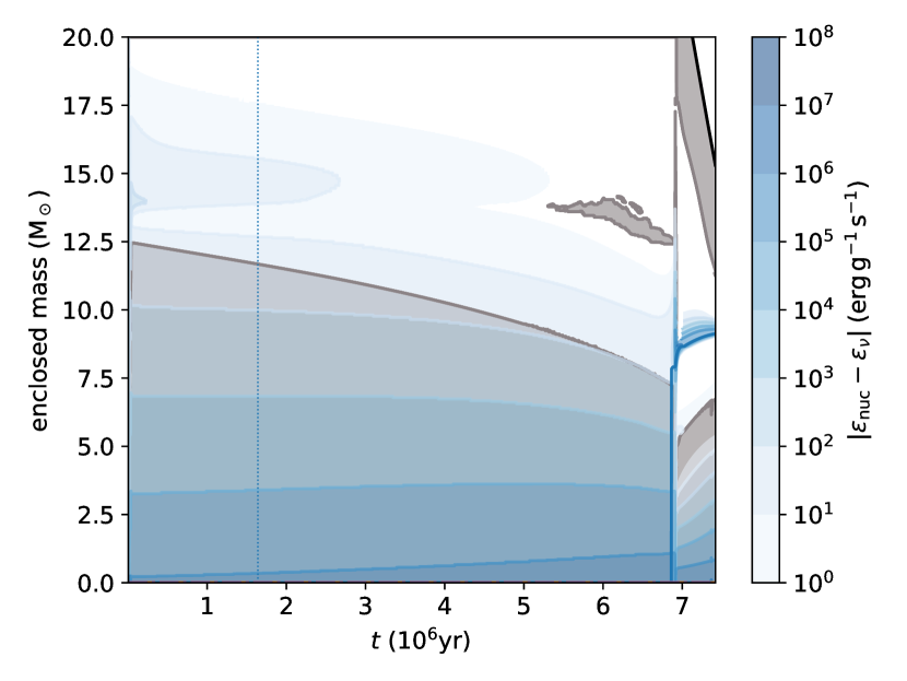
Figure 1: Kippenhahn diagram of the $25\mathrm{M}_{\odot}$ MESA stellar evolution model template from Davis et al. (2018) during H-burning core-convection phase. The vertical dotted line shows the time of model 4000 that has been used for the initial stratification of the 3D hydro simulations shown in this paper.

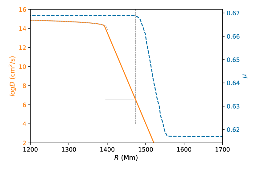
Figure 2: Profile of the diffusion coefficient and mean molecular weight $\mu$ of the MESA model from which the base state for the 3D hydrodynamic simulations is derived. Shown is the convective boundary region. The solid, horizontal black line indicates the range from the convective boundary according to the Schwarzschild condition ($r_{\mathrm{SB}}=1395\mathrm{M}\mathrm{m}$) to $r_{\mathrm{SB}}+0.18\mathrm{H_{P0}}$ where $\mathrm{H_{P0}}=417.8\mathrm{M}\mathrm{m}$ is the pressure scale height at $r_{\mathrm{SB}}$. The vertical dashed line marks the approximate radius to which the exponential CBM has mixed species essentially completely. The time of the model is indicated in Fig. 1 with a vertical dotted line.

The base state is constructed from the $25\mathrm{M}_{\odot}$ MESA stellar evolution model (time step 4000 of the template run from Davis et al., 2018) $1.64\times 10^{6}\mathrm{yr}$ after the start of H burning on the zero-age main sequence (Fig. 1). The central H mass fraction has decreased to $X(\mathrm{H})_{\mathrm{c}}=0.606$ from initially $0.706$. In the MESA simulation H-core burning ends after $6.91\times 10^{6}\mathrm{yr}$.

The fact that the mass of the convective core of 1D main-sequence models is decreasing throughout the H-core burning phase (Fig. 1) determines how the convective boundary mixing model shapes the mean molecular weight $\mu$ profile at the boundary (Fig. 2). The diffusion coefficient profile reflects efficient convective species mixing inside the Schwarzschild boundary and the decrease of the mixing coefficient according to the exponential boundary mixing model outside the Schwarzschild boundary. For the H-core burning phase the template model Davis et al. (2018) adopted $f_{\mathrm{ov}}=0.022$. The effectiveness of convective boundary mixing depends on how fast the boundary is changing its location. For a given Lagrangian boundary velocity a certain part of the exponential CBM region is essentially instantaneously mixed. For a faster moving boundary this layer is smaller. The relationship between the progression of the convective boundary and the mixing properties of exponential convective boundary mixing has already been described in detail by Herwig (2000) in the context of the formation of the ${{\mathrm{}}}{{\mathrm{{}^{13}}}}{\mathrm{C}}$ pocket for the $s$ process at the bottom of the convective envelope in AGB stars and the modeling of the third dredge-up phenomenon. In Fig. 2 the instantaneously mixed layer outside the formally convective core is indicated by the horizontal solid line and this region has an extent of $\approx 0.18\mathrm{H_{P0}}$. The boundary of the instantaneously mixed layer is indicated by the vertical dashed line. The $\mu$ gradient above the dashed line is due to two processes. In the immediate vicinity of the dashed line the profile is the result of the exponential mixing, but the bulk of this profile is due to the receding core convection. It reflects the history of the core shrinking, which in turn is impacted by the assumed value for $f_{\mathrm{ov}}$ in the stellar evolution model. In this work we show that the region of the $\mu$ gradient hosts a particular set of internal gravity waves that is associated with mixing. The $\mu$ gradient is a dominant contribution to the $N^{2}$ profile, where $N$ is the Brunt-Väisälä frequency. It is useful to keep in mind what the origin of this $\mu$ profile and thus the $N^{2}$-peak profile in the underlying 1D model is.

Another point deserves explanation. According to the exponential convective boundary mixing model, the region outside the Schwarzschild boundary obeys the radiative temperature gradient. This assumption stems from the original work by Freytag et al. (1996) who based their analysis on the shallow surface convection of white dwarfs and A-type stars. Whether or not this assumption is appropriate in the deep interior is uncertain. Recent idealized simulations (Anders et al., 2022) in plane-parallel geometry that ignore the $\mu$ gradient suggest that if applied to a $25\mathrm{M}_{\odot}$ stellar model, a very large penetration zone forms over timescales corresponding to $60,000$ convective turn-over times, much longer than the thermal time scale of the envelope of this $25\mathrm{M}_{\odot}$ stellar model ($\approx 5000$ convective turn-over times). The question of the temperature gradient in the convective boundary layer may be constrained in the future by asteroseismology (e.g.  Michielsen et al., 2019; Michielsen et al., 2021). But in any case it requires including radiation diffusion. We plan to report on such simulations in the future (Mao et al., 2023, Paper III) and just note that the results reported here for the dynamic response to the adopted MESA base state do not change qualitatively when radiation pressure and diffusion are added. In our 3D simulations we assume that the entire instantaneously mixed core up to the location where $\nabla\mu\neq 0$ (indicated by the dashed vertical line in Fig. 2) is adiabatically stratified. In other words, initially and contrary to the 1D model the entropy and $\mu$ gradient are assumed to be the same across the convective boundary except where they have to diverge where the $\mu$ gradient becomes zero outside the core, yet the entropy gradient remains positive, see Fig. 3 just above $\approx 1550\;\mathrm{\mathrm{M}\mathrm{m}}$. As the simulations progress the $\mu$ and entropy gradients can decouple depending on the relative strength and physical processes of species and heat mixing or diffusion, the latter due to radiation (not included here) or numerical effects.

2.1.2 Constructing the 3D base state

The radiation pressure fraction is $\approx 20\%$ throughout the stellar model in the core and the envelope with the exception of the outermost $\approx 300\mathrm{M}\mathrm{m}$, where it amounts to $\approx 50\%$. In the 3D simulations presented in this work, we adopt the ideal gas equation of state and ignore the radiation pressure. With this assumption we plan to establish a baseline of idealized simulation results in the same spirit as Jones et al. (2017), from which we can establish the impact of adding additional physics, such as radiation pressure, in the future.

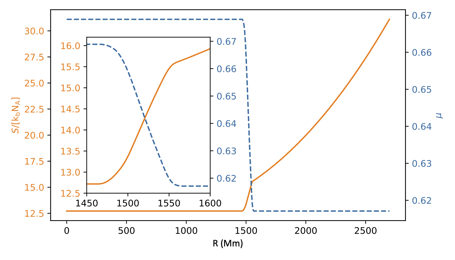
Figure 3: Entropy $S$ and mean molecular weight $\mu$ 1D stratifications (cf. Fig. 2) adopted as the base state for the 3D hydrodynamic simulations. Entropy is given in terms of code units. The PPMstar code units are length $L=10^{8}\mathrm{c}\mathrm{m}$, mass $M=10^{27}\mathrm{g}$, time $T=\mathrm{s}$, and temperature $\Theta=\mathrm{K}$.

We construct the base state or initial stratification of our simulations as follows. We use the MESA density, temperature, and mean molecular weight $\mu$ profile and calculate the entropy profile according to the assumed ideal gas EOS. We then smooth the S and $\mu$ profiles (see below) and enforce a zero gradient for entropy in the core. This determines the central pressure. The density and pressure profiles of the base state then follow from requiring hydrostatic equilibrium and mass conservation together with the equation of state.

Quantities that represent derivatives, such as the Brunt-Väisälä frequency $N$, are usually quite noisy when using a default MESA inlist file, unless special care is taken to optimize for smooth stratification profiles (e.g. Michielsen et al., 2021). However, such smoothing measures may reflect stellar physics assumptions that are uncertain and that the 3D hydrodynamic simulation is supposed to reveal. Any given 1D stellar evolution profile carries assumptions about turbulent and IGW mixing, CBM mixing, and how the turbulence and wave motions are interacting with radiative diffusion. Certain properties of the 3D simulation may depend sensitively on the assumptions made to construct the 1D base state from a stellar evolution model, while others may be more robust. Ultimately an iterative process involving parameter studies with different physics assumptions and careful analysis is required to disentangle these complex interrelations, which are beyond the scope of this paper. In view of this complication to constructing a base state for the 3D simulations, we adopt an approach in which we take the MESA profile as it is calculated with standard assumptions and then apply a smoothing procedure in a post-processing step (see §A for details). The resulting base state definition consists of the central pressure and the entropy $S$ and mean molecular weight $\mu$ profiles (Fig. 3).

Because the radiation pressure contribution is ignored, not all state variables can match the MESA profile. This is a common problem when mapping between 1D and 3D simulations with different equation of state assumptions. One can only select two variables to match the other state. Our 3D base state matches the entropy and the $\mu$ profiles of the 1D MESA profiles in the transition from the top of the convection zone and throughout the envelope because these two quantities determine the stability of the stratification. There is still some freedom in selecting the central conditions. In our base state, the central pressure and density are $20\%$ and $15\%$ smaller while the temperature is $17\%$ larger than in the MESA model. Additional technical details and a comparison with the MESA profiles are given in appendix §A.

2.2 Stellar hydrodynamics simulations

We use the PPMstar gas dynamics code (Woodward et al., 2015; Jones et al., 2017; Woodward et al., 2019; Andrassy et al., 2020; Andrassy et al., 2022), with several important updates. This version solves the conservation laws in terms of perturbations with respect to a base state. As a result, the computation can be carried out in 32-bit precision and at high accuracy. The other update relates to an improvement of how accurately mixing at the convective boundary is treated. In the past, our simulations had often focused on the ingestion of small amounts of material from the stable layer into the convective layer, and great care had been taken to advect correctly such small amounts of entrained material. In the main-sequence simulations it is however equally important to understand how much convective core material is mixed outward into the stable layer. Therefore, envelope fluid concentrations close to one are now treated equally accurately as those close to zero.

The nuclear energy input from H burning that drives the convection is represented by a constant volume heating with a Gaussian profile in the radial direction that matches the heating profile in the MESA model.

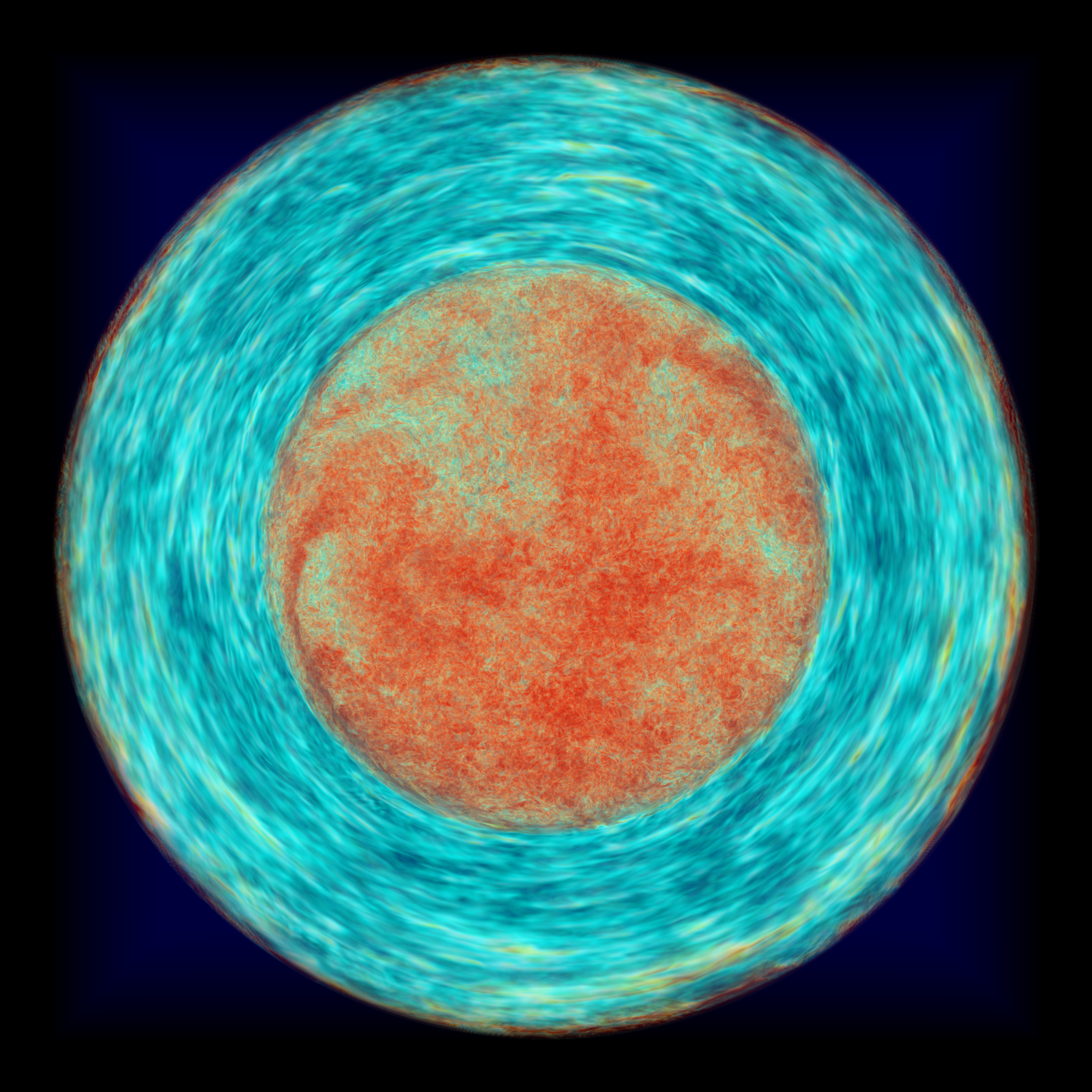
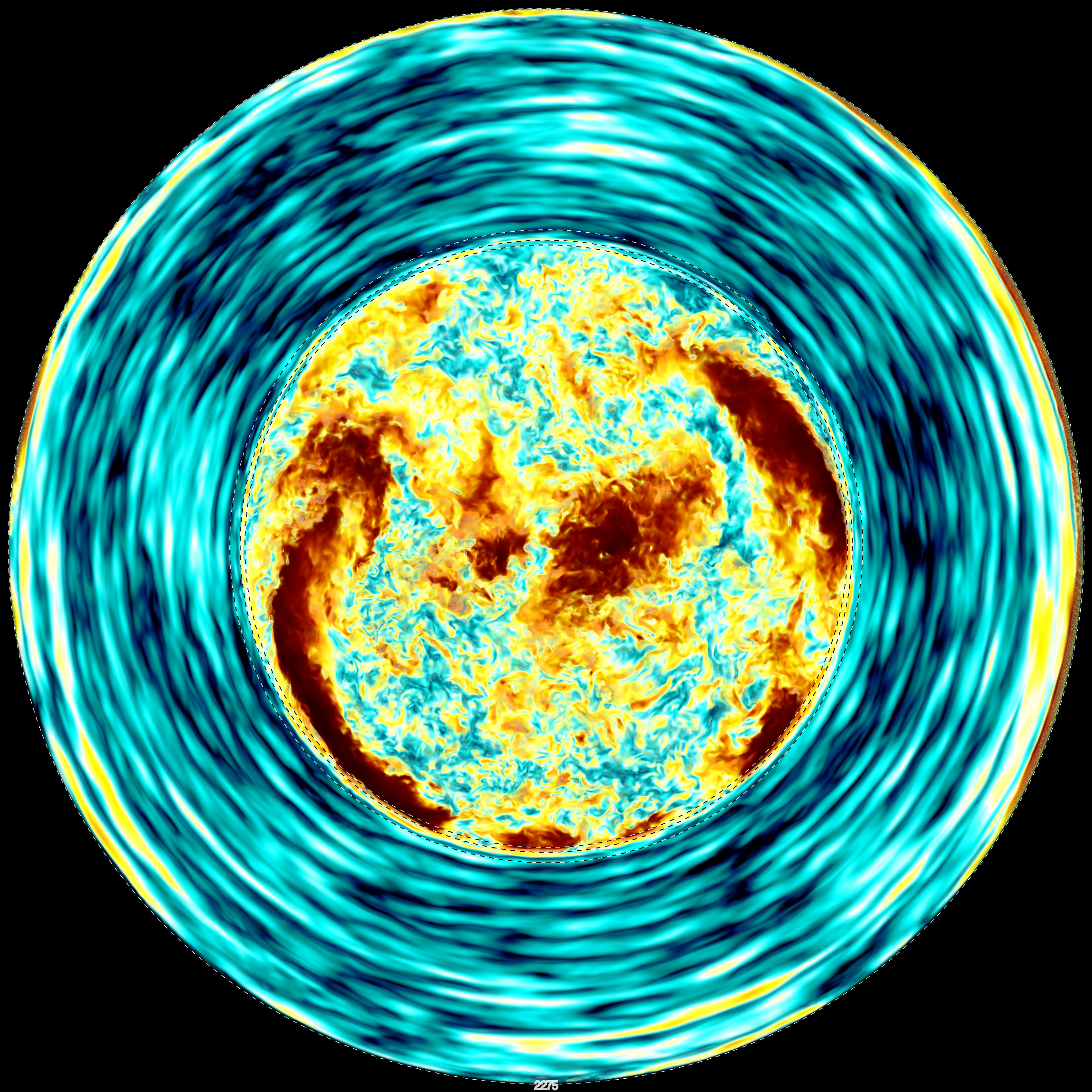
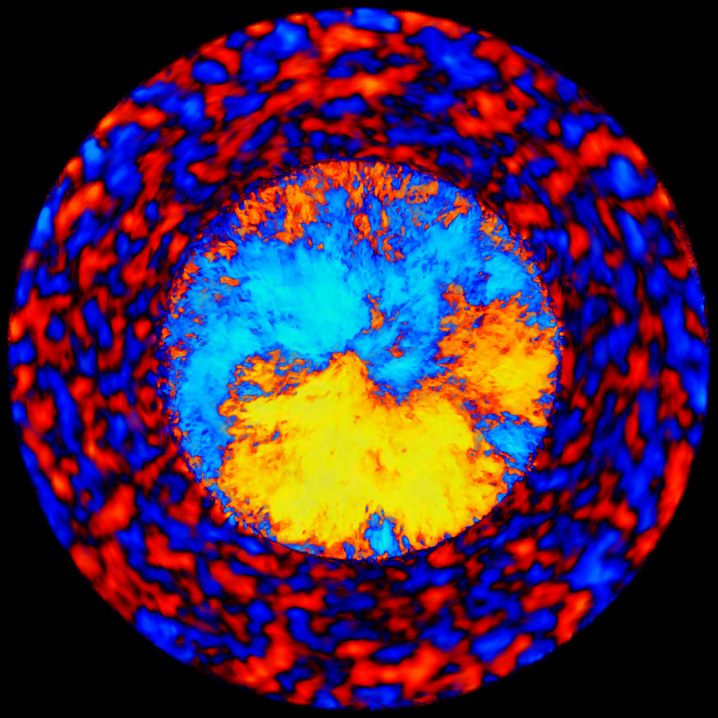
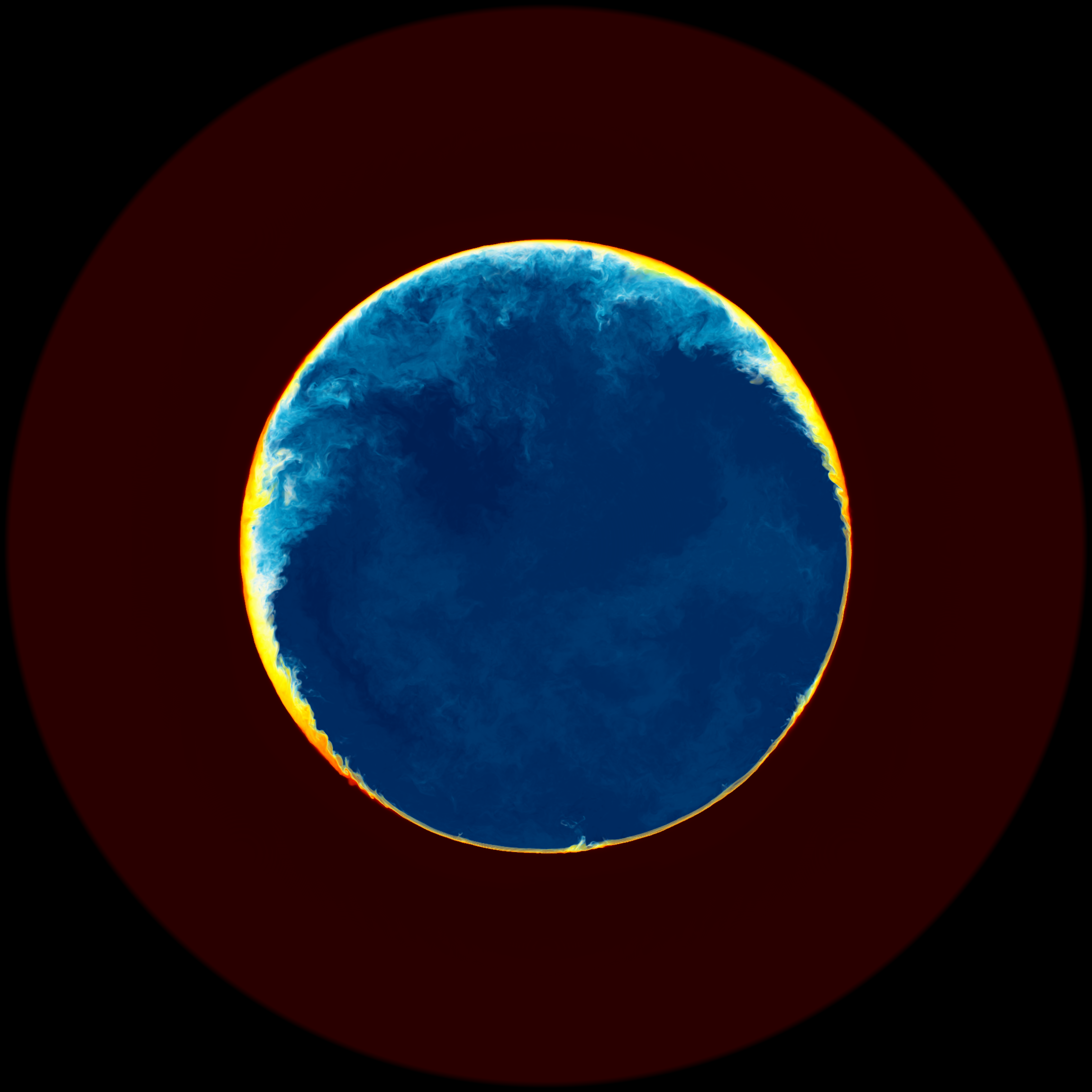
Figure 4: Renderings of vorticity (left top, from red to yellow, white, light and darker blue represents decreasing magnitudes of vorticity), horizontal velocity magnitude (right top, the same color sequence as for vorticity represents decreasing magnitudes of the horizontal velocity component), radial velocity magnitude (bottom left, blueish colors are inward motions, red-orange colors are outward directed flows), and fractional volume of the material initially only in the radiative zone of a central slice at $t=1615.25\mathrm{h}$ (dump 2275) from simulation M115 ($1728^{3}$ grid). These images have non-linear color and transparency maps intended to bring out important flow patterns as clearly as possible. The images are not intended to provide a quantitative scale, which can instead be derived from line plots such as Fig. 5 and Figs. 7 and 8. Movies and full-resolution images of these quantities are available at https://www.ppmstar.org.

PPMstar performs its computations in Cartesian coordinates using a uniform 3-D grid of cubical grid cells. This structure of the computation optimizes numerical accuracy for a general fluid flow problem. It also gives rise to a simple and highly effective design in which the computation proceeds in symmetrized sequences of 1-D passes in the 3 coordinate directions, a procedure called directional operator splitting. One consequence of our coordinate choice is that the application of boundary conditions becomes more difficult. We generally place the grid boundaries at radii that are well removed from the action that is under study. Boundary conditions are implemented at specific radii, an inner radius (or optionally no inner radius) and an outer radius. Because we place these bounding spheres well away from the region of study, we handle them in ways that make their implementation easy. It is important to realize that we do not attempt to apply our boundary conditions on truly spherical surfaces. Instead, we approximate the sphere by the nearest set of cubical grid cell faces. This means that the bounding sphere is ragged at the scale of the grid. Since the grid is made fine enough to faithfully compute the fluid flow, this raggedness of the bounding spheres is usually not a concern, especially since they are located well away from the convection zone. When studying core convection, we have no inner bounding sphere, and the outer one, given the Cartesian grid, is better resolved than any spherical surface inside it. At the bounding sphere we impose a reflecting boundary condition. This is imposed using ghost cells that mirror the cells across the bounding surfaces. This is done in each 1-D pass, and in each such pass the bounding surface is perpendicular to the direction of the pass, but it is not perpendicular to the gravitational acceleration vector. For our convenience, we therefore smoothly turn off gravity beginning a few grid cell widths in radius before the bounding sphere is reached. This allows us to implement a trivially simple boundary condition in each 1-D pass. The cost of this approach is that we introduce a very thin layer in which the gravitational acceleration smoothly drops to zero right next to the boundary. In the simulations we have performed with this code to date, this has caused no noticeable problems. If one is only interested in the convection flow and the behavior near the convective boundary or boundaries, this approach is easily defended. If one is also interested in studying the internal gravity waves that are excited by the convection and that propagate in the stably stratified regions outside it, the reflection properties of the gravity waves at the boundaries, if those boundaries are reached by the waves, could matter. Any impact this approximation may have on our results would be revealedin the resolution study we typically do on any problem we work on.

We perform simulations for a range of heating rates and grid resolutions. Simulations with different grid resolutions allow some estimate about the numerical convergence properties. In most cases it is sufficient to determine if simulations are approaching convergence under grid refinement, i.e. does the ratio of quantities of interest become smaller for equal ratios of grid refinement. If this is the case, a simulation series with different grid sizes gives an indication of the accuracy of quantitative results.

All of our simulations have a larger driving luminosity compared to the nominal energy generation rate of the $25\mathrm{M}_{\odot}$ stellar model. This is necessary because at nominal heating the Mach number $\mathcal{M}$ of the convective flow is very small. According to the MLT velocities from the MESA template model the average is $\mathcal{M}\approx 5\times 10^{-4}$. Prohibitively small computational grid cells would be required for accurate simulations. Recall that the PPMstar code is an explicit gas dynamics code, and although it is optimized to efficiently perform low-$\mathcal{M}$ number stellar convection simulations, there is a natural limit for what can be expected of any such numerical approach. We vary the heating factor from $10^{1.5}$ to $10^{4}$. Such a heating series allows us to extrapolate relevant quantities to the nominal heating of the simulated star (Table 1).

Table 1: Summary of simulations used in this paper. Given are the run ID, number of grid zones in each dimension, the length of the simulated time in hours, the heating factor compared to the nominal luminosity of the 1D stellar model and the number of convective turnovers $N_{\mathrm{conv}}$ computed. For the latter the length of the run from column three is divided by the convective turnover time for $1000\times$ heating runs of $128\;\mathrm{\mathrm{h}}$ (cf. §3.1.1) scaled according to $U_{\mathrm{conv}}\propto L^{1/3}$ (cf. §5.1).

ID	grid	$t_{\mathrm{end}}/\mathrm{h}$	$\log L/L_{\mathrm{\star}}$	$N_{\mathrm{conv}}$
M109	768	885	4.0	14.9
M118	1152	905	4.0	15.2
M108	768	1414	3.5	16.2
M119	1152	1414	3.5	16.2
M107	768	7049	3.0	55.1
M114	1152	4189	3.0	32.7
M115	1728	2473	3.0	19.3
M111	2688	1355	3.0	10.6
M106	768	3472	2.5	18.5
M100	1152	1531	2.5	8.1
M105	768	2847	2.0	10.3
M116	1152	2885	2.0	10.5
M110	768	2155	1.5	5.3
M117	1152	3370	1.5	8.3

As in previous work (Andrassy et al., 2020; Stephens et al., 2021), the analysis is based on three different types of output from the PPMstar code. In these main-sequence simulations, detailed outputs that we call dumps are written to disk every $42.6\mathrm{min}$ of star time (in most of the simulations discussed here) which corresponds to $\approx 400$ time steps on a $768^{3}$ grid and correspondingly more on the larger grids. For each dump, radial profiles of spherically averaged quantities are written out as well as briquette data that contains relevant derived quantities, such as the vorticity, calculated from the full-resolution grid and then averaged to a 3D grid that is four times smaller in each Eulerian grid dimension. This filtered data is of high quality and can usually be analyzed conveniently in a post-processing step. The third output type are the 3D full resolution byte-sized data cubes used to generate images. A number of default images are also written out for convenience during the simulation at each dump.

2.3 Wave analysis

A key analysis of our simulations is to determine the oscillation properties of our 3D simulations. Paper II is dedicated to a comprehensive wave analysis of these simulations, including predictions of asteroseismic observations. Here we use the wave analysis to identify fluid motions due to IGWs in the layers immediately above the convection zone, as these may be relevant for the convective boundary mixing as discussed in §4.3.

In brief, our wave analysis consists of two parts. We determine the vibrational modes present in the simulations to generate a frequency-wavenumber diagram by post-processing the 3D briquette (cf. §2.2) velocity data. The GYRE code (Townsend & Teitler, 2013; Townsend et al., 2018) searches for eigenfrequencies of standing wave modes for a specified value of $l$ and a range of $n$. We calculate eigenfrequencies of IGWs for spherical harmonic degrees $1\leq l\leq 50$ and radial orders $n\in[-1\dots-20]$ according to the 1D spherically averaged stratification of the 3D simulation using GYRE. By comparing the GYRE predictions with the spherical harmonics decomposition of the 3D simulation, we can identify the dominant presence of certain IGWs in the 3D simulation and ascertain the wave nature of the fluid motions.

First, we decompose each of 2000 dumps into spherical harmonics using the SHTools library. We then take the discrete Fourier transform of each spherical harmonic coefficient after applying a Hanning window to control spectral leakage. Finally, for each frequency bin, we compute the spherical harmonic power spectrum normalized by degree $l$. This results in a grid of power spectral density as a function of temporal frequency and spherical harmonic degree $l$, the $l-\nu$ diagram. It can then be compared to the theoretical dispersion relations and calculations from GYRE.

To calculate properties of IGW modes from the radial profiles of the spherically averaged stratification for a given dump of a 3D simulation with the stellar oscillation code GYRE, the radial profile data from the 3D simulation is transformed to the MESA input format readable by GYRE as explained in Paper II. By tuning the control parameters of the GYRE code, we have been able to determine the spherical harmonic degree $l$ from 1 to 50, finding g-mode oscillations of the orders $n$ from -1 to -20, f modes, and a few low-radial order p modes. The results of this analysis are described in §4.3. Throughout this paper, $N$ is the angular Brunt-Väisälä frequency.

2.4 Mixing analysis

We determine radial diffusion coefficient profiles by feeding appropriately averaged radial abundance profiles into the inversion of the diffusion equation and determine the profile $D(r)$ that would have been needed in 1D to generate the observed evolution of abundance profiles from spherically and time-averaged 3D data as first introduced by Jones et al. (2017). The method is based on comparing angle-averaged radial profiles of composition at two points in time with some time averaging applied around both endpoints to suppress statistical noise. The transformation from the first profile to the second is then assumed to be due to a diffusive process, and the diffusion coefficient is derived by inverting an appropriate discrete diffusion equation. The most important updates as compared to Jones et al. (2017) are: (1) we formulate the diffusion equation using the mass coordinate as an independent variable and (2) we take the star’s spherical geometry into account. The mapping from Eulerian to mass coordinates becomes important where mixing is slow and differences between the two composition profiles become dominated by 1D compression and expansion of the stratification.

We will critically interpret the IGW mixing results obtained in this way in terms of mixing due to IGWs inducing shear mixing (e.g. Denissenkov & Tout, 2003, and references therein) in the general framework of shear-induced mixing by small-scale turbulence (Garcia Lopez & Spruit, 1991; Zahn, 1992a; Prat et al., 2016). In this picture, IGWs are generating shear motions reflected in magnitude by the vorticity acting against the stabilizing effect of positive Brunt-Väisälä frequency. For $\omega\ll N$, the IGW fluid motion is nearly horizontal with a vertical velocity shear

$$\frac{du_{\mathrm{h}}}{dr}\approx u_{\mathrm{h}}k_{\mathrm{v}}\approx u_{\mathrm{h}}k_{\mathrm{h}}\left(\frac{N}{\omega}\right)\mathrm{\,,}$$

where $u_{\mathrm{h(v)}}$ is the horizontal (vertical) velocity component, $k_{\mathrm{h(v)}}$ the horizontal (vertical) wave number, $\omega$ the wave frequency, and $N$ the buoyancy frequency (Garcia Lopez & Spruit, 1991).

The diffusion coefficient for shear-induced mixing by small-scale turbulence has been estimated by Zahn (1992b) as

$$D_{\mathrm{shear}}\approx\eta\frac{\left(\frac{du_{\mathrm{h}}}{dr}\right)^{2}}{N^{2}}K{}$$ (1)

where

$$K=\frac{4acT^{3}}{3\kappa\rho^{2}C_{\mathrm{P}}}{}$$ (2)

is the thermal diffusivity and $\eta\approx 0.1$. Using the definition of the Richardson number $Ri$ (Eqn.  8.13, Shu, 1992, §B)

$$Ri=\frac{N^{2}}{(du_{\mathrm{h}}/dr)^{2}}{}$$ (3)

the diffusion coefficient is

$$D_{\mathrm{shear}}\approx\eta\frac{K}{Ri}{}$$ (4)

This estimate of shear-induced mixing is supported by 3D hydrodynamic simulations by Prat et al. (2016) for horizontal velocity shear artificially set up in a box. If the Richardson number in Eq. (4) exceeds its critical value $1/4$, the vertical variation of the horizontal velocity of IGW oscillations is stable for adiabatic fluid motion. Through radiative heat losses, perturbed fluid elements can lose some of their entropy memory and shear instability can develop even when $Ri>1/4$ (Townsend, 1958), provided that the viscosity is too small to stabilize it. Zahn (1974) proposed a new instability criterion that takes into account a finite viscosity, according to which shear mixing may occur when $Ri\,Pr\la 10^{-3}$ (Garaud, 2021). For extremely low Prandtl numbers $Pr=\nu/K\ll 1$ in stellar interiors, e.g. for $Pr\sim 10^{-6}$ in the radiative envelope of our $25\mathrm{M}_{\odot}$ model, such instability and shear-induced mixing may develop at relatively large values of $Ri\la 10^{3}$.

The horizontal components of the vorticity of the IGW fluid motion can be estimated as

$$(\nabla\times\mathbf{u})_{y}=\frac{\partial u_{x}}{\partial z}-\frac{\partial u_{z}}{\partial x}\approx u_{\mathrm{h}}k_{\mathrm{v}}-u_{\mathrm{v}}k_{\mathrm{h}}\approx u_{\mathrm{h}}k_{\mathrm{h}}\frac{N}{\omega}\ ,{}$$ (5)

or $(\nabla\times\mathbf{u})^{2}_{y}\approx(u_{\mathrm{h}}k_{\mathrm{h}})^{2}\left(\frac{N}{\omega}\right)^{2}\approx(u_{\mathrm{h}}k_{\mathrm{v}})^{2}$. A similar estimate can be obtained for the x component of the vorticity. If the total vorticity magnitude $|\nabla\times\mathbf{u}|$ is dominated by the horizontal vorticity magnitude $|\nabla\times\mathbf{u}|_{\mathrm{h}}$ (as is the case in our simulations, §5.2), then $(u_{\mathrm{h}}k_{\mathrm{v}})^{2}\approx(\nabla\times\mathbf{u})^{2}$ and

$$D_{\mathrm{IGW}}\approx\eta\frac{(\nabla\times\mathbf{u})^{2}}{N^{2}}K{}$$ (6)

which implies in this case $Ri\approx\frac{N^{2}}{|\bm{\nabla\times}u|^{2}}$. The factor $\eta$ of order unity reflects the specific type of shear motion. It has been determined for specific flow morphologies from hydrodynamic simulations (Prat et al., 2016; Garaud et al., 2017). The exact morphology of IGW-induced instabilities is not yet clear, and it therefore remains to be shown if these calibrations can be applied directly in this case. We apply these concepts to interpret IGW mixing efficiencies measured from our 3D simulations in §5.3.

3 General flow morphology

3.1 The velocity field

An initial impression of the general flow morphology is provided by central plane slices of velocity components, vorticity, and concentration of the fluid in the stable layer shown in Fig. 4. The highly turbulent convective core with finely granulated three-dimensional distribution of vorticity is clearly distinguished from the orderly and layered motion patterns seen in the stable envelope. These regular fluid motions that are well distinguished in both velocity components and in the vorticity are dominantly IGWs, as we demonstrate in detail in Paper II.

3.1.1 The dipole dominating the convective core

The largest scale motion in the convection zone is the single dipole mode that is best seen from the radial velocity image. For the dump shown in Fig. 4, the dipole is almost exactly aligned along the north-south direction. It is well known that the largest scale mode of a convectively stratified layer fills the largest vertical size of the convection zone. For a fully convective non-rotating sphere, this mode is the dipole (Jacobs et al., 1998; Porter et al., 2000; Kuhlen et al., 2003). Our core convection simulations are no different in that regard. Only non-spherical macro physics processes such as rotation may break up this symmetry (Woodward et al., 2022, Paper IV).

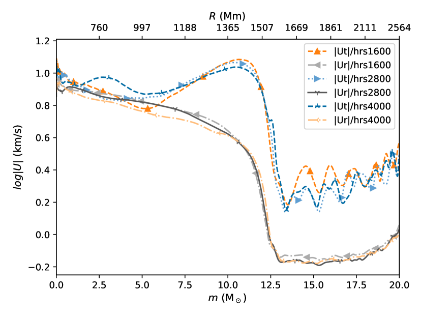
Figure 5: Radial and tangential velocity component of run M114 ($1000\times$ heating, $1152^{3}$ grid). For each velocity component three different times are shown to demonstrate the typical amplitude of fluctuations.

The large-scale dipole flow passes right through the centre and diverges when reaching the boundary in this case near the south pole. The convective fluids return to the downflow origin at the antipode located near the north pole in a sweeping tangential flow along the convective boundary along both the east and west meridians. The visualization of the tangential velocity magnitude (Fig. 4) resembles the shape of a horseshoe (dark red indicating the largest tangential velocity magnitudes) that is aligned with the convective boundary and open to the north. At about the location of the equator for the flow along the western meridian and about $30\deg$ further north along the eastern meridian, the tangential boundary layer flow starts to separate from the boundary and begins to develop an inward-directed velocity component. The flow forms a characteristic wedge in these locations that is also seen in the vorticity image.

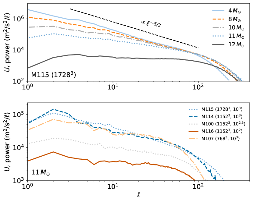
Figure 6: Top panel: Spectra of deep core and core close to boundary show how the turbulent spectrum changes from Kolmogorov to flat (the legend gives the mass coordinates where each spectrum was calculated). The power in the radial velocity component is binned as a function of the spherical harmonics angular degree $\ell$, and the spectra are averaged over dumps 1900 to 2300. Bottom panel: Spectra at a fixed mass coordinate but with different grid resolutions (see legend) as well as for lower heating rates. The same dumps as in the top panel are used.

In Woodward et al. (2015), we have identified this boundary layer separation region as the key feature that facilitates the entrainment of fluid from the stable layer into the convection zone for the case of the upper boundary of He-shell convection in a low-mass star. Boundary-layer separation is a basic phenomenon in fluid dynamics and described in introductory textbooks (e.g. Kundu & Cohen, 2008). Flow separating from a boundary experiences additional nonlinear instabilities that resist analytical descriptions. However, the reason for the separation of the flow from the boundary is straightforward. The $\mathcal{M}$ number of the simulated convection, for example in simulation M114 ($1000\times$ heating factor, $1152^{3}$ grid) is $\mathcal{M}\approx 0.015$ with maximum values reaching $0.06$ in some locations near the convective boundary. At such low $\mathcal{M}$ numbers, the flow is nearly incompressible. Momentum conservation dictates that a flow against an opposing pressure gradient has to develop a perpendicular velocity component. In this case, the opposing pressure gradient originates from the opposite tangential boundary-layer flow heading toward the origin of the downdraft. The outward-directed perpendicular flow direction is prohibited by the stiff convective boundary and therefore only the inward-directed perpendicular flow is possible. Because of the low $\mathcal{M}$ number, this boundary separation starts already at a large distance away from the antipode near the north pole, where the centre of the downdraft is located. As we discuss below, the boundary-layer separation wedges are where the entrainment of material from the stable layer into the convective core takes place. The wedges are also a key mechanism in exciting IGWs (Paper II).

Finally, for later use it is useful to specify a convective timescale. If we adopt for the $1000\times$ runs an average convective velocity of $U_{\mathrm{conv}}\approx 6.5\mathrm{k}\mathrm{m}/\mathrm{s}$ (Fig. 5) and adopt as convective crossing distance the diameter of the convective dipole to be $2R_{\mathrm{conv}}\approx 3000\;\mathrm{\mathrm{M}\mathrm{m}}$ then the convective time scale is $128\mathrm{h}$ (or $\approx 180$ dumps).

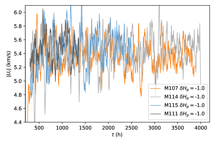
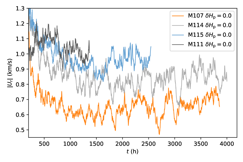
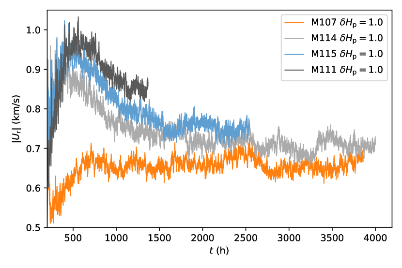
Figure 7: Spherically averaged radial velocity magnitude time evolution for grid resolutions $768^{3}$ (M107), $1152^{3}$ (M114), $1728^{3}$ (M115), and $2688^{3}$ (M111, cf. Table 1) at $r_{\mathrm{N^{2}-peak}}\pm\mathrm{H_{P0}}$ (labels $\pm\delta H_{\mathrm{p}}$), where $r_{\mathrm{N^{2}-peak}}$ is where $N^{2}$ has a maximum in the boundary region and $\delta H_{\mathrm{p}}$ is in units of $\mathrm{H_{P0}}$. At $r_{\mathrm{N^{2}-peak}}$ $\mathrm{H_{P0}}=349\mathrm{M}\mathrm{m}$ or $4.6\mathrm{M}_{\odot}$ at $t=1662\mathrm{h}$ of simulation M115.

3.1.2 Radius dependence of the velocity spectrum in core convection

The global dipole nature of the flow is also revealed in spherically averaged radial and tangential velocity component profile plots shown in Fig. 5. The convective boundary is located approximately at mass coordinate $12.5\mathrm{M}_{\odot}$ (cf. §4.3 for more details on the determining the location of the convective boundary more accurately). Near the convective boundary inside the convection zone ($7.5\mathrm{M}_{\odot}$ to $12.5\mathrm{M}_{\odot}$), the tangential velocity component is up to $50\%$ larger than the radial velocity. This broad peak of the tangential velocity magnitude represents the sweeping circular boundary layer flow from where the dipole approaches the boundary toward the antipode where the downdraft originates. Correspondingly, the radial velocity component continuously decreases toward the boundary with peak values found in the central region of the convective core. This asymmetry between radial and tangential velocity components is similar to what shell convection shows where the tangential velocity magnitude peaks both just below the upper boundary and above the lower boundary (Jones et al., 2017; Andrassy et al., 2020; Stephens et al., 2021).

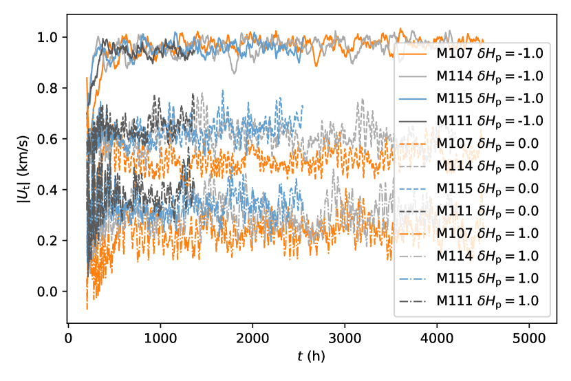
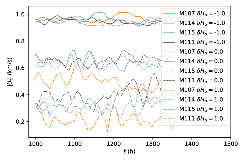
Figure 8: Similar to Fig. 7 for the tangential velocity component, except in decimal logarithms.

The change of the convective flows from radial-component dominated in the deep core and tangential-component dominated near the boundary has important consequences for power spectra of convective motions that break down radial velocity by spherical harmonic degree $l$. In the deep core, the scales from the large dipole mode to the the smallest homogeneous turbulent motions assume a turbulent spectrum in which the largest scales dominate (Fig. 6). However, closer to the boundary, large-scale radial motions are suppressed compared to the deeper layers, simply because they do not fit into the smaller remaining vertical distance to the stiff convective boundary. The spectrum of $U_{\mathrm{r}}$ becomes flatter and the relative importance of smaller-scale motions increases. At or just below the convective boundary the spatial radial velocity spectrum is indeed flat. Interestingly, the spatial spectrum of the horizontal velocity component remains $\propto l^{-5/3}$ near the boundary, and even into the stable layer (cf. §4.2).

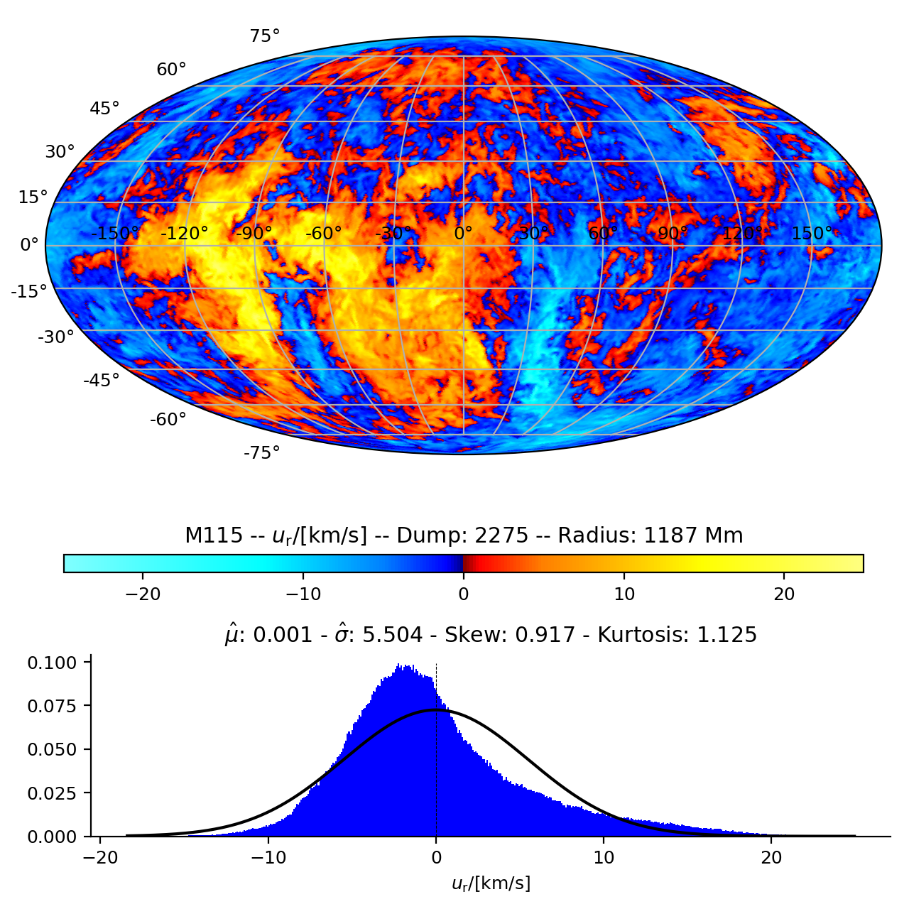
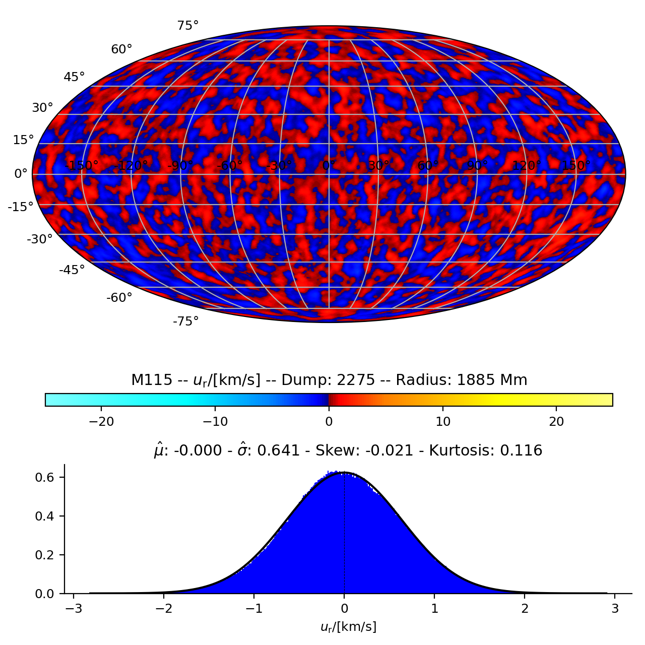
Figure 9: Mollweide projections of the radial velocity component and probability distribution function on the $4\pi$ sphere for run M115 ($1728^{3}$-grid). Left: For radius $r=r_{\mathrm{N^{2}-peak}}-\mathrm{H_{P0}}=(1536-349)\mathrm{M}\mathrm{m}=1187\mathrm{M}\mathrm{m}$ in the convective core. Right: For $r=r_{\mathrm{N^{2}-peak}}+\mathrm{H_{P0}}=(1536+349)\mathrm{M}\mathrm{m}=1885\mathrm{M}\mathrm{m}$ in the stable envelope. The radius $r_{\mathrm{N^{2}-peak}}$ is at or just above the convective boundary as discussed in §4.3. The black solid lines are Gaussians fitted to the PDFs. Labels provide the values for the moments mean, standard deviation, skew, and excess kurtosis.

This change of the spectrum of scales from the central region of the convection zone to the boundary has already been noted for the case of He-shell flash convection in rapidly-accreting white dwarfs by Stephens et al. (2021), who used this spectral profile information from the 3D simulations to feed a reduced-dimensionality advective mixing and nucleosynthesis post-processing scheme. The centre-plane images in Fig. 4 reveal that the boundary-layer separation wedges described above are locations where motions of all scales including very small scales originate. This spectrum of motions is also an important ingredient in modeling the excitation of IGWs. One key result is that the immediate convective region below the boundary is not dominated by a few low wave numbers, but rather power of the radial velocity component is almost equally distributed over a wide range of represented scales.

3.1.3 Wave motions in the stable envelope

The time evolution over long and short periods of radial and tangential velocity components in the core, boundary, and envelope region is shown in Figs. 7 and 8. The amplitudes of the tangential velocity component waves in the envelope are larger by about a factor $\approx 2.5$ than those of the radial component in both temporal and spatial dimension (see also Fig. 5), as expected for IGWs.

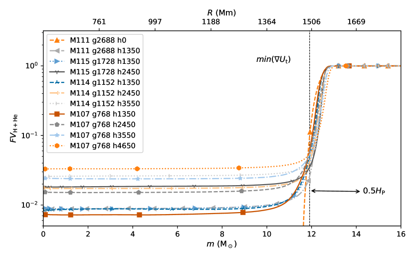
Figure 10: Fractional volume of the fluid in the stable layer (H+He) for three grid resolutions at different times. The vertical dashed line shows the location where the radial gradient of the tangential velocity has a minimum ($\min d|U_{\mathrm{t}}|/dr$) in run M107 at $t=1600\mathrm{h}$, which can be taken as the location of the convective boundary (see §4 for a discussion of where the convective boundary is located).

Both the tangential and the horizontal velocity component ultimately adopt a steady-state in which neither velocity component changes nor drifts noticeably as a function of time. The $768^{3}$-grid simulation M107 has been followed for $7059\;\mathrm{\mathrm{h}}$ and does not show a trend of the velocity magnitude in the envelope beyond the time shown in Figs. 7 and 8.

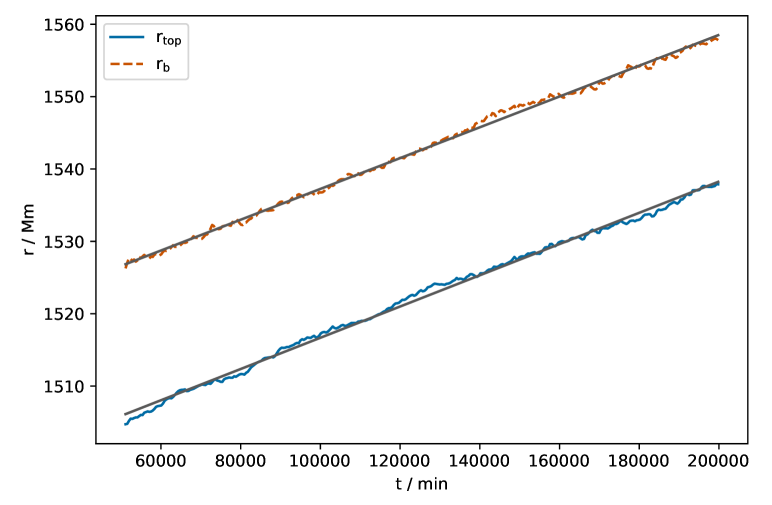
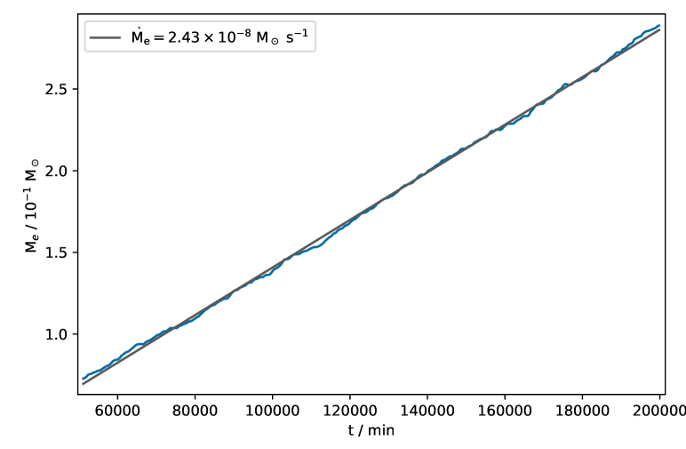
Figure 11: Time evolution of the convective boundary radius (top panel). Shown is the radius $r_{\mathrm{b}}$ where $\max dFV/dr$ and the radius $r_{\mathrm{top}}$ which is one $FV$ scale height further inward ($r_{\mathrm{top}}=r_{\mathrm{b}}-H_{FV}$). The mass integration is carried out to $r_{\mathrm{top}}$. A linear fit of the resulting entrained mass evolution (bottom panel) yields the entrainment rate.

For the tangential velocity component, the initial transient to reach this steady state is of the order of a convective turn-over time (see also discussion in §5.2). The radial component appears to go through a longer transient period of $\approx 1500\;\mathrm{\mathrm{h}}$ until it settles into the steady state value. This longer time scale is also the time it takes for the boundary to migrate through the initial $N^{2}$ profile due to mass entrainment (cf. discussion in §2.1.1 and results in §4.1). Possibly the radial velocity component is more sensitive to the exact shape of the boundary in the $N^{2}$-peak region.

The time-evolution comparison of results obtained from simulations on different grid sizes indicates that velocity component magnitudes and their oscillation properties are essentially in good agreement among the different grid resolutions. Only the $768^{3}$-grid results diverge by a small amount in predicted envelope velocities.

3.1.4 Statistics of convective and wave motions

Another way to visualize the fundamental difference between the flow patterns in the core and the envelope is to use velocity images on spheres of constant radius. Fig. 9 shows such images for the radial velocity component for a radius well inside the convection zone and a radius one pressure-scale height above the convection zone in the stable layer. These projection images onto a sphere reveal large and coherent upflow areas and somewhat more narrow downflow lanes. Smaller-scale structures are distributed throughout the sphere and blur the distinction between up- and downflow areas. In the stable layer, smaller regions of upward- and downward-directed flow are ordered in a semi-regular fashion. This difference can be expressed quantitatively through the probability distribution function (PDF) shown below each image and its higher-order moments. The convective PDF has a large skew, meaning it has significant asymmetry compared to a Gaussian. There are more units of area on the sphere with downflows than upflows. However, the largest radial velocities are found in areas with upflows rather than downflows. The relative strength of the far tail is measured by the excess kurtosis. Large values of kurtosis indicate an overabundance of far-tail events. Turbulent convection is intermittent with gusts of larger-than-average flow speeds occurring at random times. This is reflected in the larger kurtosis compared to the PDF of the stable envelope.

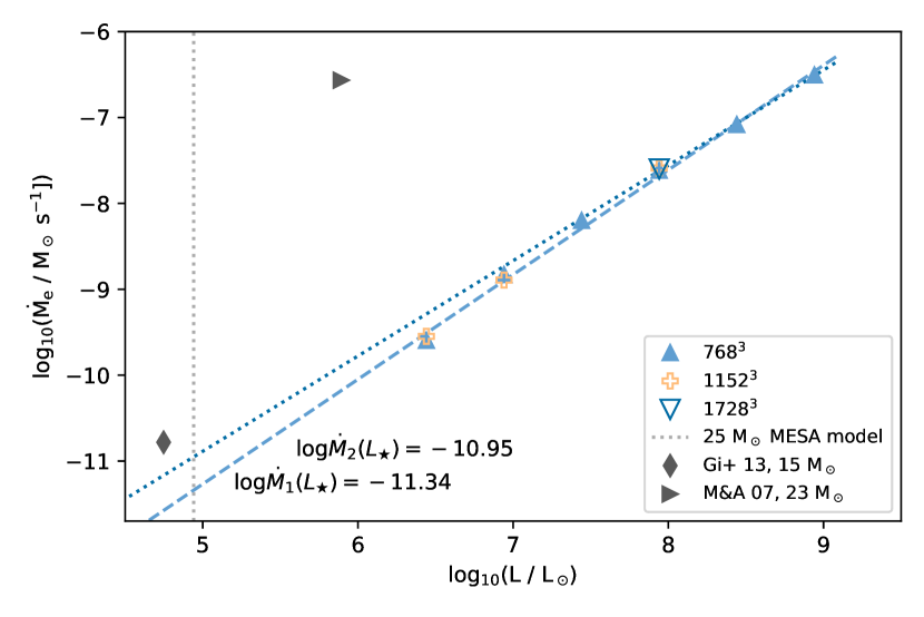
Figure 12: Entrainment rates as a function of driving luminosity for runs with different grid resolutions as indicated in the legend. Two linear fits are provided. Fit $\dot{M}_{1}$ (dashed line) is based on the highest resolution run available for each heating rate. The second fit (dotted line) includes only the $768^{3}$ grid runs for the three highest heating rates. Fit parameter uncertainties are standard deviations of the fitting only. The vertical grey dotted line indicates the nominal luminosity of the underlying 1D MESA model. The intercept values of both fits with the nominal heating ordinate are indicated as well as the entrainment rates reported by Gilet et al. (2013) and Meakin & Arnett (2007) for similar simulations.

The PDF of radial velocities in the envelope on the other hand is represented almost perfectly with a Gaussian distribution. Anticipating the presentation of the spectra of IGWs in the boundary region in §4.2 and in the entire envelope (Thompson et al., 2023, Paper II), we note that the IGWs in the stable layers of these simulations have power in the radial velocity component peaking at spherical harmonic degree $l\approx 30$ and that IGWs with all eigenfrequencies below the Brunt-Väisälä frequency are well-represented. As demonstrated elsewhere in more detail, the coherent superposition of this wide range of IGW eigenmodes results in a Gaussian PDF. This feature of the $U_{\mathrm{r}}$ PDF is thus a quantitative symptom of a velocity field dominated by IGWs. We use this statistical difference between convective and wave motions in §4.3 to characterize the motions in the convective boundary region.

3.2 Entrainment

In §3.1.1 we discussed the fluid morphology of the giant dipole modes and the intimately related boundary-separation wedges. The orientation of the dipole drifts as the simulation proceeds, which can be best observed by watching the movies. This drift time scale is that of several convective turnovers of $\approx 128\;\mathrm{\mathrm{h}}$ (§3.1.1). The convective boundary is stiff, and at the location where the uprising flow impacts the radial position of the convective boundary it is only minimally displaced. At the boundary, the flow is redirected from a radial to a dominantly horizontal component. The large impact zone of the outward flow of the dipole approaching the boundary at the south pole in Fig. 4 would be the closest thing to what one might consider a plume in these simulations. However, the southern hemisphere where this impact takes place is not where the entrainment takes place. The bottom-right panel in Fig. 4 shows the concentration of the material initially only in the stable layer that we refer to as the H+He fluid.

The instabilities induced by the boundary-layer separation flows that we call the wedge features are responsible for the entrainment of material from the stable layer into the convection zone. This is evident by comparing the velocity centre-plane images (Fig. 4) with the image of the H+He fluid, where orange, yellow, and white colors indicate partially-mixed zones. These regions of effective entrainment are located opposite to each other on the boundary circle near the east and west equator coordinates. The dipole axis is tilted a bit to the west in the dump shown. The dominant hydrodynamic mechanism of entrainment is here, as it was in He-shell flash convection (Woodward et al., 2015), the instabilities induced by boundary-layer separation of large-scale flow sweeping along the convective boundary.

The continuous entrainment process leads to an accumulation of H+He fluid in the convective core. Spherically averaging the H+He concentration leads to profiles as shown in Fig. 10 for the three different grids used in the $1000\times$ heating simulations. After $4000\mathrm{h}$, or $31$ convective timescales ($128\;\mathrm{\mathrm{h}}$, §3.1.1) the H+He stable-layer fluid has accumulated to a level of $\approx 3\times 10^{-2}$ in the convective core.

Integrating over the H+He fluid concentration from the centre to the convective boundary gives the total entrained mass. With respect to the upper boundary for the entrained mass integration, we use a similar approach as Jones et al. (2017), but instead of the minimum gradient of the tangential velocity component we adopt here the maximum gradient of the H+He fractional volume $FV$ reduced by one $FV$ scale height. This is essentially equivalent to integrating to the radius at which $FV=0.1$. Using $FV$ instead of $U_{\mathrm{t}}$ gives a smoother boundary evolution for main-sequence simulations because the $\min d|U_{\mathrm{t}}|/dr$ criterion often finds a location just outside the dynamic boundary that is dominated by the $n=-1$ IGWs (§4.2). The entrained H+He mass evolves linearly with time, and examples are shown in Fig. 11 for simulations with different grid resolutions and heating factors. In each case, the initial transient ($\approx 300$ to $\approx 1000\mathrm{h}$) of the simulation was discarded for the purpose of fitting a linear relation to the entrainment evolution. During this initial transient, the entrained mass as a function of time would still show non-linear behaviours that can in part be understood in terms of the evolution of the convective boundary profile as a function of time and heating factor as discussed in §4. This fit of the entrained mass determines an entrainment rate for each simulation. For simulations of O-shell convection in massive stars, we have previously found a linear relation between the heating factor and the entrainment rate (Jones et al., 2017; Andrassy et al., 2020). Fig. 12 shows the entrainment rates for all heating factors and grid resolutions included in this paper.

For a few heating factors, we have carried out simulations for multiple grid resolutions. The entrainment rate does not depend systematically or significantly on grid resolution for our simulations. Next, we note that again, as in O-shell simulations, the entrainment rates follow a linear trend over a wide range of heating rates. Two linear fits are shown in Fig. 12. One includes only the three highest heating rates $1000$, $3162$, and $10000$, while the other fit includes all heating rates.

Either way the resulting mass entrainment rate at nominal heating is unrealistically large, $\approx 5\times 10^{-12}\;\mathrm{\mathrm{M}_{\odot}/\mathrm{s}}$ for the second fit. This is $992\mathrm{M}_{\odot}$ applied over the H-core burning lifetime of $6.91\times 10^{6}\;\mathrm{\mathrm{yr}}$. This interpretation of the derived entrainment rate obviously does not make sense. Our simulations are not alone in predicting very large entrainment rates, but in good agreement with those of Gilet et al. (2013), who used a low-$\mathcal{M}$ number solution scheme. They include radiation pressure but like us ignore radiative diffusion. Meakin & Arnett (2007) report an entrainment rate about three orders of magnitude higher than our simulations and included both radiation pressure and radiation diffusion. Preliminary tests that we will describe in detail in a forthcoming publication indicate that neither the addition of radiation pressure, radiative diffusion or the addition of rotation resolves the unrealistically high entrainment rate. Instead, the strong time-dependence of the response of the 3D hydrodynamic simulation to the adopted MESA base state signals that the initial MESA base state is out of thermal-dynamic equilibrium in the 3D hydro framework. The large entrainment rate leads to an increasing nearly-adiabatic layer outside the initial convective boundary. Thus the large entrainment rate phase of these 3D simulations represents the approach toward a thermal-dynamic equilibrium state with a larger nearly-adiabatic core. Our own preliminary tests and simulations by Anders et al. (2022) show that indeed such simulations reach a quasi-equilibrium state.

4 The convective boundary

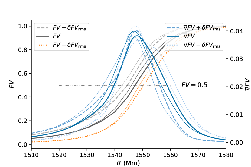
Figure 13: FV profiles (left ordinate) and FV gradients from FV spline interpolations of FV (right ordinate) at the boundary for $2450\;\mathrm{\mathrm{h}}$ (thick lines) and $2350\;\mathrm{\mathrm{h}}$ (thin lines), run M115 ($1000\times$ heating factor, $1728^{3}$ grid)

.

Figure 14: Radial profile of Brunt-Väisälä frequency for low heating factor runs (Table 1).

An important goal of this paper is to improve our understanding of the hydrodynamic processes and properties of the convective boundary. In this section, we describe the properties of the boundary, how to determine its location, and the different types of motions in the boundary region. Again, an important aspect is to demonstrate how the results depend on grid resolution. We will focus the discussion on the $1000\times$ simulations, for which simulations with four grid resolutions have been used (M107 – $768^{3}$, M114 – $1152^{3}$, M115 – $1728^{3}$ and M111 – $2688^{3}$).

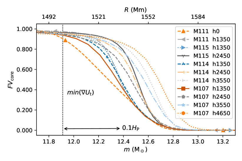
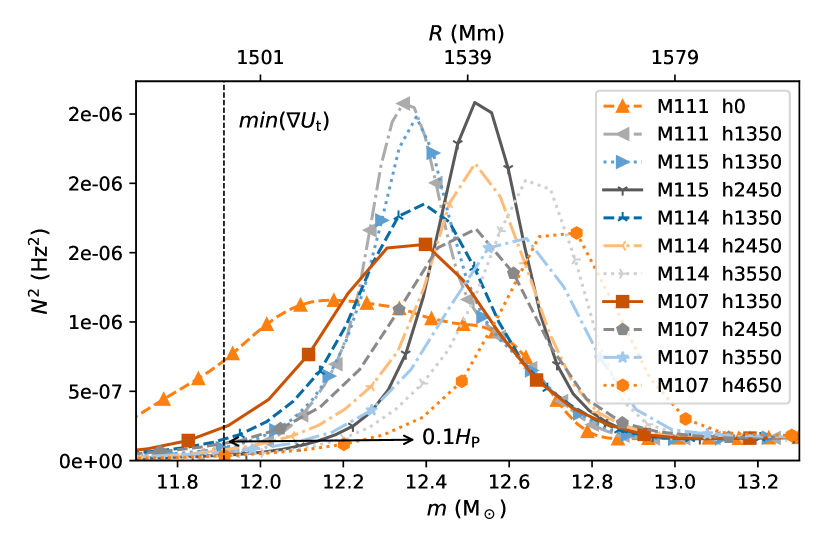
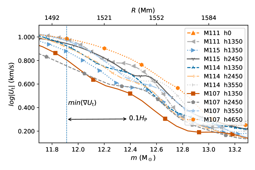
Figure 15: Radial profiles of the core fluid, $N^{2}$, and the magnitude of the tangential velocity component. The legend gives the run ID (Table 1), the grid size, and the time in hours. Markers are shown every three data points. The vertical line shows for run M107 and $1350\;\mathrm{\mathrm{h}}$ the location of the minimum (steepest) gradient of the tangential velocity component, which is one of the criteria for the boundary of the convection zone (cf. §4.3). For reference the size of $0.1\mathrm{H_{P}}$ is shown with a horizontal arrow. The abscissa at the top gives the radius according to $r(m)$ for $1350\;\mathrm{\mathrm{h}}$ of run M107, see text for details.

4.1 Evolution of the boundary in terms of spherical averages

Radial profiles of 3D simulation quantities averaged on spheres are an obviously useful dimensional reduction when the goal is to develop models for applications in 1D stellar evolution codes. We are mentioning two complications. The first is that because we keep heating the core at rates that are much larger than the nominal heating rate, and we do not include radiation diffusion (simulations with radiative diffusion will be presented in Paper III Mao et al., 2023), the core is expanding and thereby the radial coordinate of the boundary is moving slightly. This effect is easily taken care of by working with radial profiles in terms of the mass coordinate.

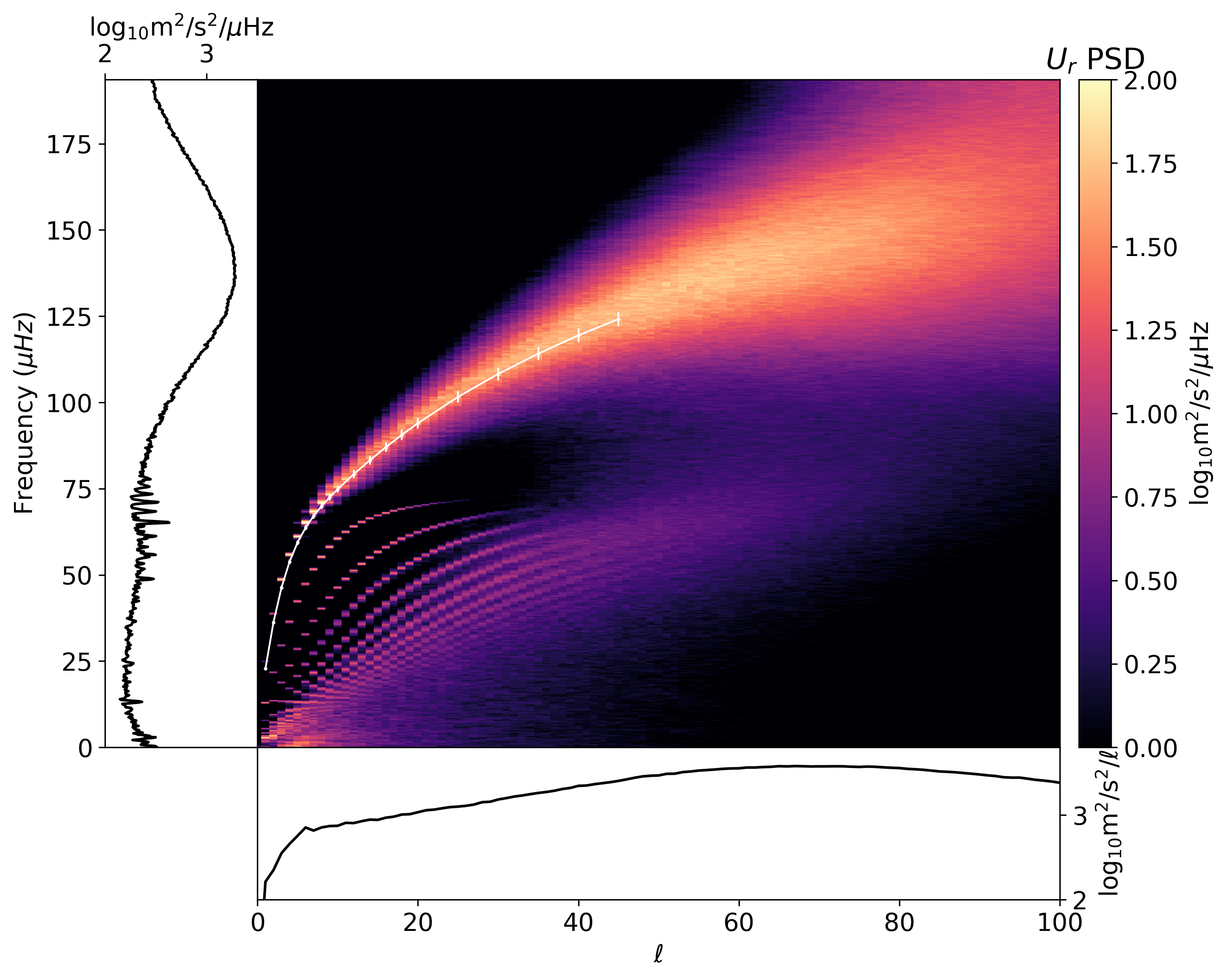
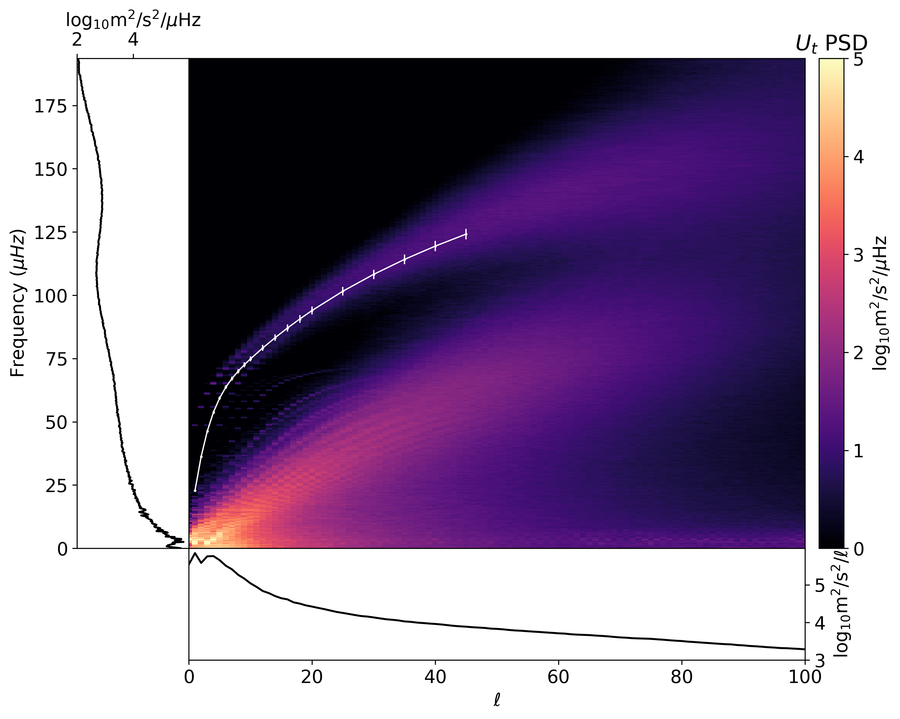
Figure 16: Power spectral density as a function of spherical harmonic angular degree $l$ and cyclic frequency ($l-\nu$ diagram) for the radial (top) and horizontal (middle) velocity components in simulation M114 ($1000\times$, $1152^{3}$ grid) at $r=12.6\mathrm{M}_{\odot}$, where the peak of $N^{2}$ is located. Dumps 3925 to 5924 were used. The white line with dots are $n=-1$ modes determined from the GYRE calculations for the spherically-averaged stratification of dump 3925. The abscissa and ordinate include projected spectra in terms of spherical harmonic $l$ and frequency, respectively.

The second point is a bit more subtle. The boundary according to the adopted MESA base state is very stiff, which implies that the boundary layer is narrow in the radial direction. The largest-scale modes of the convection may lead to a non-spherical deformation of the position of the convective boundaries, or of certain features. When taking an average over a deformed surface, for example of the concentration, one obtains a smoothly varying profile. However, when averaging over an undeformed surface, which has for each boundary surface element a turbulently mixed interface where each vertical volume element truly consists of a mix of the two materials separated by the boundary, then the resulting averaged vertical profile is likewise a smoothly varying profile. Only in the latter case does the radial concentration profile represent partial mixing. The situation is like that of ocean swell from a distant storm on a calm day. Taking horizontal averages will yield a smoothly varying vertical profile, but nowhere except on the molecular level can there be found a volume element that contains water and air. This second aspect of radial profiles from spherical averages of 3D data is much more difficult to take into account.

An estimate for the magnitude of this effect can be obtained from the 3D spherical rms-deviations of the FV profile. Fig. 13 shows these for two times approximately one convective turnover apart, as well as their derivatives, which would correspond to the $N^{2}$ profiles. The maximum of the gradient differs by $\loa 3\;\mathrm{\mathrm{M}\mathrm{m}}$ between $FV\pm\delta FV_{\mathrm{rms}}$ profiles, whereas the radius at which $FV=0.5$ differs at both times by $\approx 5\;\mathrm{\mathrm{M}\mathrm{m}}$. Further insight into how much the dominant spherical boundary features are subject to deformation and what the internal structure of the boundary is will be explored in §4.3.

The key quantities are shown for the narrow $\approx 100\mathrm{M}\mathrm{m}$-wide boundary layer region in Fig. 14 for lower heating runs and for $1000\times$ heating factor simulations in Fig. 15. The concentration of the core material traces mixing while $N^{2}$ (which is proportional to the entropy gradient) represents the stability of the stratification, and the magnitude of the tangential velocity represents the average of the actual fluid flow. For low heating factors the initial boundary stratification (cf. §2.1) is somewhat deformed but the entrainment rate overall is too small to migrate the boundary signifcantly over the durartion of the simulation. At $1000\times$ heating rate the initial boundary structure is entirely erased after about $1000\;\mathrm{\mathrm{h}}$, as discussed already in §3.2. In these simulations, the entrainment rate is so high that the boundary migrates through the mass region of the original $N^{2}$ peak region and establishes a new $N^{2}$ profile that has no memory of the initial stratification and is only due to hydrodynamic processes. The $N^{2}$-peak becomes higher and narrower, and this trend is more pronounced for higher-resolution grids. Visual inspection of the peak $N^{2}$ values as a function of grid resolution shows that the maximum steepness of the boundary is increasing with grid resolution. This can be understood in terms of IGW mixing in the $N^{2}$-peak region decreasing with grid resolution, as explained below. The rate of boundary progression is constant and the same for each of the three grids, and it is equal to the mass entrainment rate reported in Fig. 12.

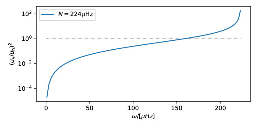
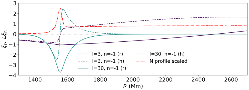
Figure 17: Top panel: Ratio of vertical to horizontal velocity component according to Eq. (8) for N at the $N^{2}$-peak location of run M114 (Fig. 15). Bottom: Radial $\xi_{r}$ and horizontal $L\xi_{\mathrm{h}}=\sqrt{l(l+1)}\xi_{\mathrm{h}}$ oscillation displacement amplitudes of two $n=-1$ modes with $l=3$ and $l=30$ calculated with GYRE for dump $3925$ of simulation M114 (cf. §2.3).

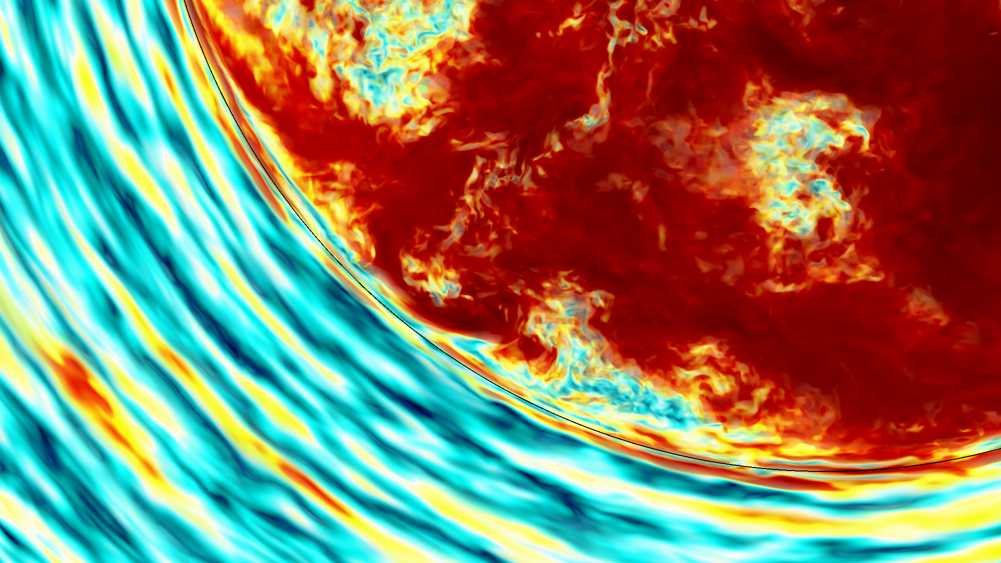
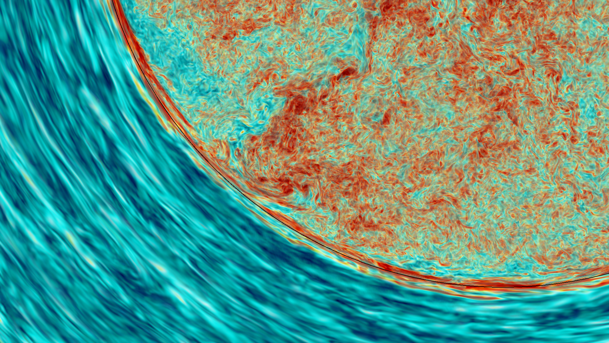
Figure 18: Zoomed-in images of the tangential velocity component (top) and vorticity magnitude in the convective boundary region from run M111 ($2688^{3}$ grid) dump 1225. The black circular lines show the radial location of the $N^{2}$-peak.

$N^{2}$ (which is $\propto dS/dr$) follows $dFV/dr$ in this transition region except where these gradients transition to different envelope values at the top of the $N^{2}$ profile. Once the $N^{2}$ peak has passed through the initial $N^{2}$-peak region given by the initial stratification, it migrates outwardly in a self-similar form. The same is true for the concentration profile which, like the $N^{2}$-peak region, has an approximate width of $0.2\mathrm{H_{P}}$, as shown in the top panel of Fig. 15. This means that mixing processes must occur on both sides of the peak of $N^{2}$ and across the entire peak region. We establish in §5 that the $N^{2}$-peak region experiences mixing due to IGWs. It then follows that the shape of the $N^{2}$-peak profile is a convolution of its migration in mass coordinate and the IGW mixing, similar to how it works for the convective boundary in a 1D stellar evolution model (second-last paragraph in §2.1.1). IGW mixing in the $N^{2}$-peak region is inversely proportional to grid resolution (§5.3.2), while the entrainment rate is essentially independent of grid resolution (Fig. 12). Therefore, the $N^{2}$-peak profile for higher-resolution runs is narrower as the simulation evolves toward quasi-equilibrium.

Jones et al. (2017) adopted the criterion $\min d|U_{\mathrm{t}}|/dr$ to locate the convective boundary. In Figs. 10 and 15 that location is shown by a vertical line for run M107 at $t=1000\;\mathrm{\mathrm{h}}$. It is also clear that the decrease of $|U_{\mathrm{t}}|$ is not monotone nor steady in many of the cases shown, as we would expect from an exponential decay of convective velocities assumed for the 1D exponential diffusive CBM model. At times, the tangential velocity component can even increase with radius, indicative of wave motions. For this reason, as discussed in §3.2, we did not adopt the $\min d|U_{\mathrm{t}}|/dr$ criterion as the entrained mass integration boundary but instead the $\max dFV/dr$ criterion.

4.2 The $n=-1$ IGW mode in the convective boundary region

In the $1000\;\mathrm{\mathrm{h}}$ profile of M107 (Fig. 15), the dashed vertical line indicates the location where the dominant convective flow velocities are dropping off rapidly. In this section, we demonstrate that the velocity field transitions rapidly above the vertical dashed line from convection-dominated to wave-dominated, and that the layers at and above $N^{2}$-peak, according to our diagnostics, are exclusively populated by wave motions.

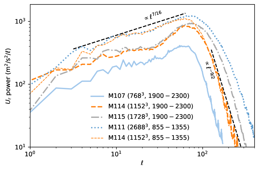
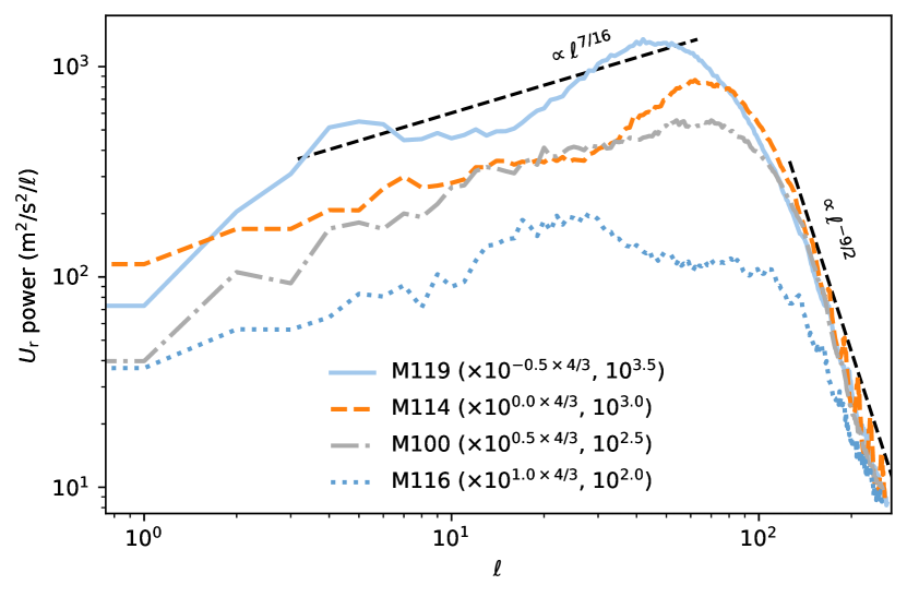
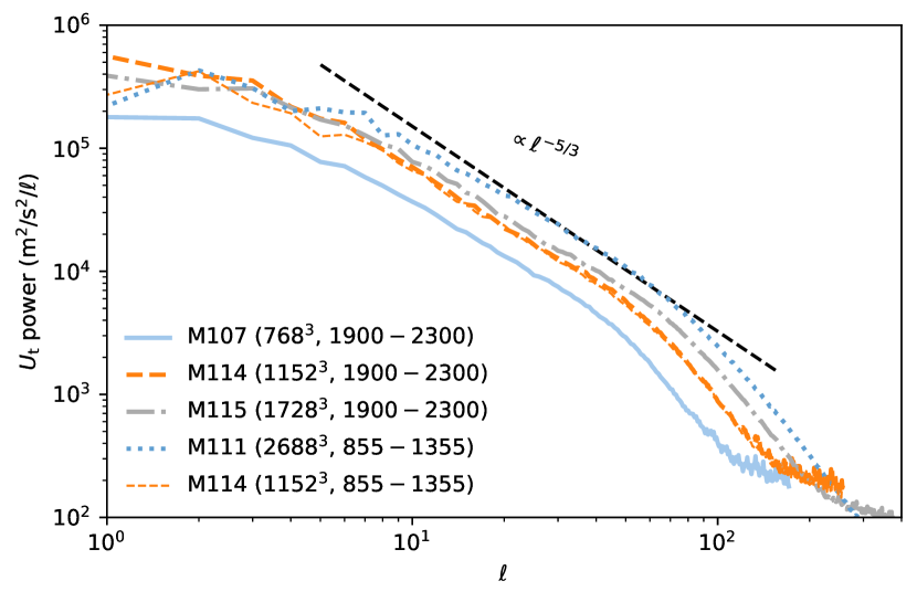
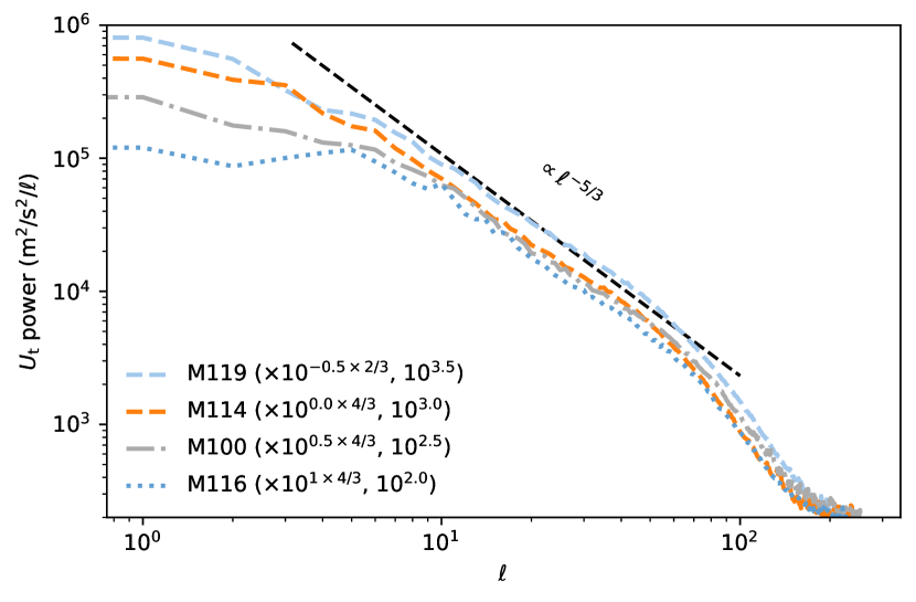
Figure 19: Spatial power spectral distribution of radial (top row) and horizontal (bottom row) velocity component for different resolutions at $1000\times$ heating factor (left column) and for different heating factors (right column, $1152^{3}$ grids) at the location of the maximum of the $N^{2}$-peak. Spectra for different heating factors are scaled according to the velocity scaling relations established in §5.2 as indicated in the legend. Various power laws are shown to guide the eye. Spectra with different boost factors shown in the right panels are also averaged over $300$ to $400$ dumps.

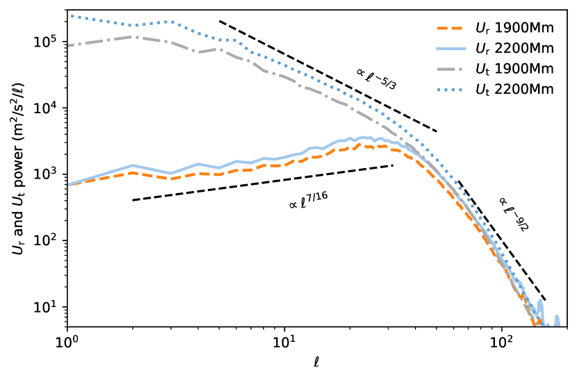
Figure 20: Horizontal and radial velocity component power spectra as in Fig. 19 for run M114 (1152-grid) averaged over dump range $1900$ to 2300 at two radii in the envelope one to two pressure scale heights above the $N^{2}$-peak location.

This is demonstrated by performing a spatio-temporal wave analysis (see §2.3 for details). $l-\nu$ diagrams for core and envelope radii are be presented by Thompson et al. (2023, Paper II). Here we focus just on the wave analysis of the immediate convective boundary layer. Fig. 16 shows the $l-\nu$ diagram derived from the 3D simulations for the $N^{2}$-peak radius along with the $n=-1$ modes predicted by GYRE for the M114 stratification.

As expected for IGWs, low-frequency modes have overall a large ratio of horizontal to vertical velocity component ($u_{\mathrm{h}}/u_{\mathrm{v}}\gg 1$). Given the kinetic energy flux of IGWs (e.g. Eq. 39 Press, 1981)

$$F_{\mathrm{IGW}}=\rho u_{\mathrm{v}}^{2}\frac{N}{k_{\mathrm{h}}}\sqrt{1-\frac{\omega^{2}}{N^{2}}}=\rho u_{\mathrm{h}}^{2}\frac{\omega^{2}}{Nk_{\mathrm{h}}}(1-\frac{\omega^{2}}{N^{2}})^{-1/2}{}$$ (7)

the frequency dependence of the ratio of the velocity components is

$$\frac{u_{v}^{2}}{u_{h}^{2}}=\frac{\omega^{2}}{N^{2}(1-\omega^{2}/N^{2})}{}$$ (8)

and shown in Fig. 17. The velocity ratio is $u_{\mathrm{v}}/u_{\mathrm{h}}>1$ for $\omega/N>0.7$ but for $\omega\ll N$ the power of the horizontal velocity component exceeds the power in the radial component by two orders of magnitude.

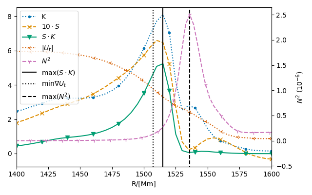
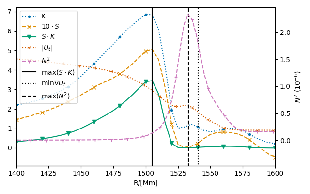
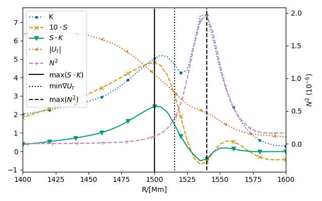
Figure 21: Radial profiles of kurtosis $K$, weighted skewness $S$ (scaled a factor of $10$ for visibility), their product $S\cdot K$, the norm of the tangential velocity $|U_{\mathrm{t}}|$, and the Brunt-Väisälä frequency $N^{2}$ in units of $\mathrm{rad/s}$. Top: M115 at $1615.25$hr (dump 2275 shown in Figs. 4 and 22); middle: M115 at $1444.15$hr ; bottom: M114 at $1619.5$hr.

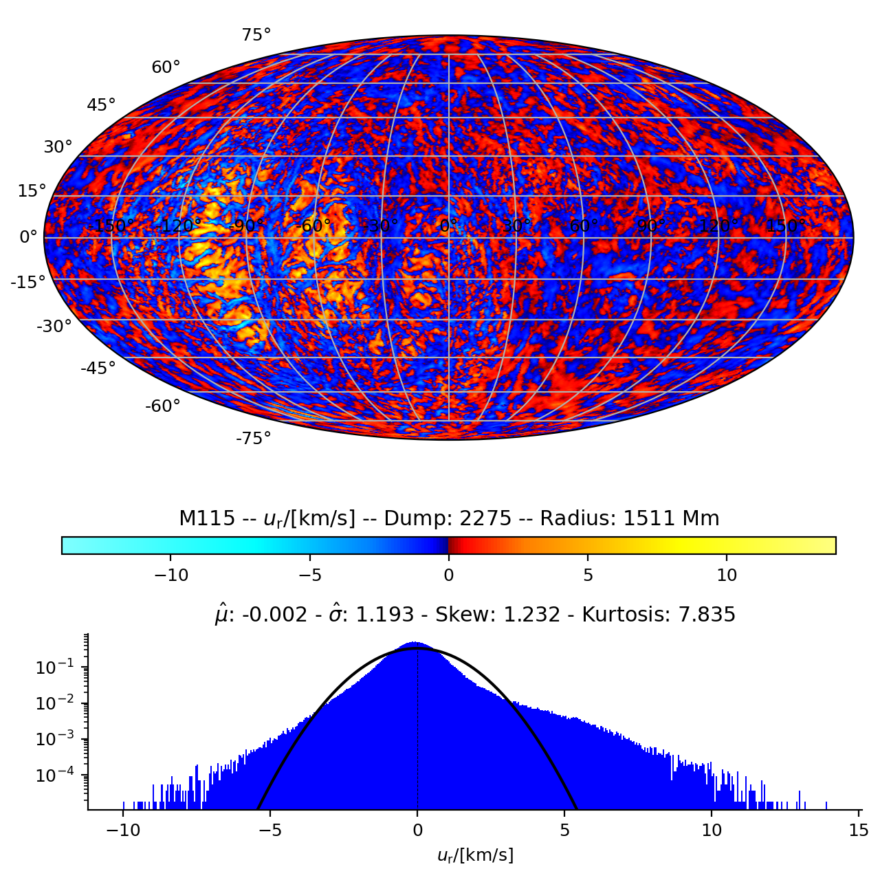
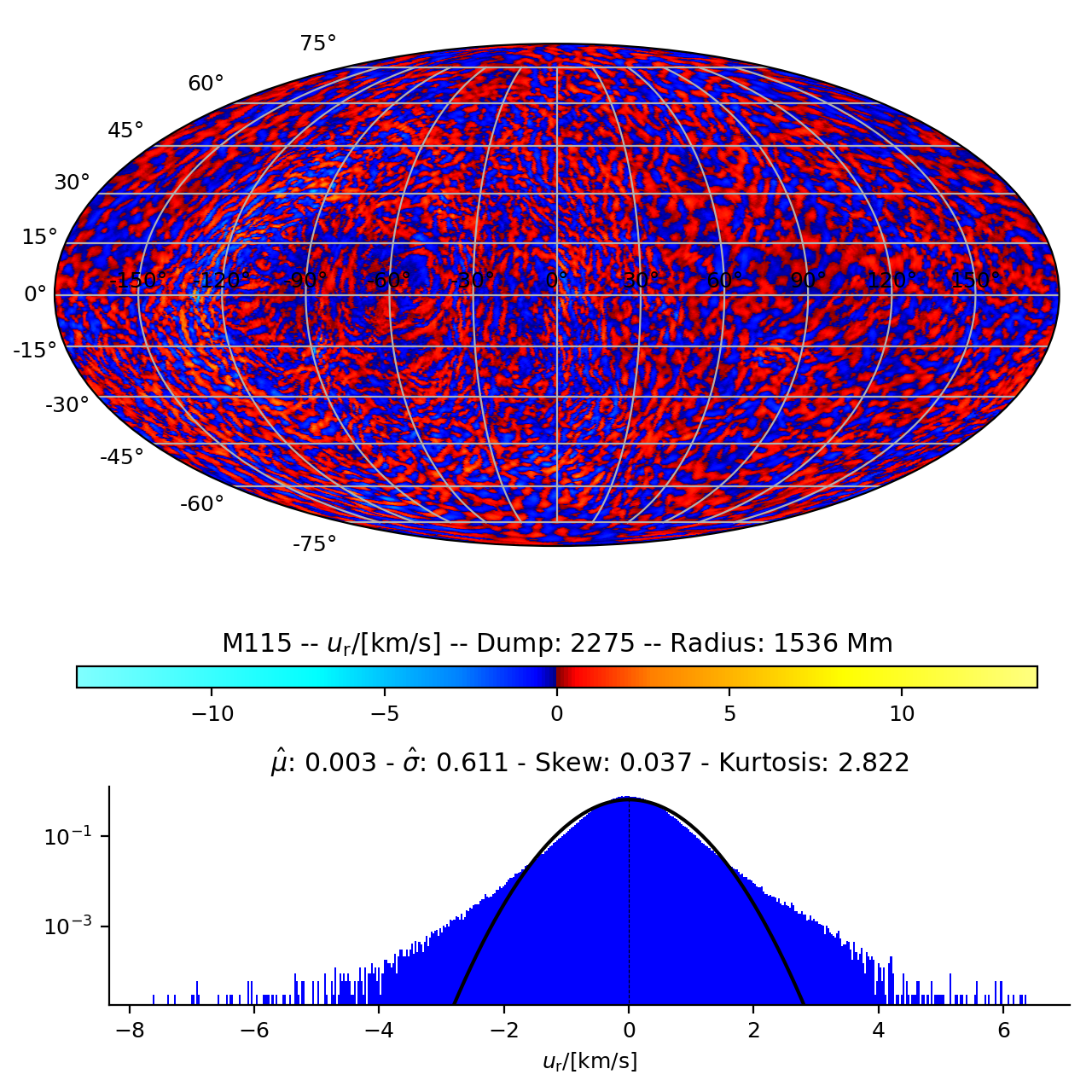
Figure 22: Mollweide projections of the radial velocity component and PDF on the $4\pi$ sphere. Left: At the location of the convective boundary according to the K-S-product-peak criterion at $r_{\mathrm{KS-peak}}=1511\mathrm{M}\mathrm{m}$. Right: At the location of the peak of $N^{2}$ at $r_{\mathrm{N^{2}-peak}}=1536\mathrm{M}\mathrm{m}$.

The power spectral distribution shown in $l-\nu$ diagrams for the radial and horizontal velocity components (Fig. 16) reflect this expectation that $U_{\mathrm{t}}$ is overall larger than $U_{\mathrm{r}}$ power. The power in the radial component $U_{\mathrm{r}}$ is dominantly associated with the $n=-1$ mode at high $l$. At low frequencies, a much smaller amount of power is associated with higher $n$ modes. The $U_{\mathrm{r}}$ power is largest at high $l\geq 50$ and high frequencies $f\approx 140\;\mathrm{\mu\mathrm{Hz}}$. This frequency is much higher than the convective frequency, which is $\approx 2.5\;\mathrm{\mu\mathrm{Hz}}$ at $1000\times$ heating. Power associated with convective motions is found in the lower-left corner at $f\leq 50\;\mathrm{\mu\mathrm{Hz}}$ and $l\leq 60$ (Fig. 13 Thompson et al., 2023, Paper II). The $U_{\mathrm{r}}$ $l-\nu$ diagram shows essentially no power that could be associated with those frequencies. The $U_{\mathrm{t}}$ power on the other hand is dominantly concentrated in eigenmodes with low frequencies and correspondingly low wave numbers.

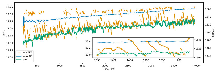
Figure 23: Time evolution of the mass coordinate of the maximum of the skew-kurtosis product $SK$, the steepest radial gradient of the tangential velocity component $\min d|U_{\mathrm{t}}|/dr$ and the peak of the squared Brunt-Väisälä frequency $\max(N^{2})$ for simulation M114 ($1152^{3}$) and, in the inset, more detail from the M115 simulation ($1728^{3}$). These three quantities mark the location of the convective boundary in different ways, see text for discussion.

Fig. 17 (bottom panel) shows the radial and horizontal components of the displacement amplitude of two $n=-1$ modes from the GYRE calculation, for $l=3$ and $l=30$. The high-$l$ modes have peaks of opposing direction bracketing a node at the $N^{2}$ peak location. The $l=3$ mode as an example for a low-$l$ mode also has a sign change in the horizontal velocity component at the $N^{2}$-peak radius. This means that these IGW modes have horizontal components exactly opposite right above and below the $N^{2}$-peak location, where the radial component has a single maximum. For high $l$ values, the mode amplitude is sharply peaked in and around the narrow $N^{2}$-peak region and falls off quickly both outwardly in the stable layer and inwardly in the convectively unstable layer.

Inspection of centre-plane horizontal-velocity component slices (Fig. 18) immediately reveal these $n=-1$ modes and specifically the nodal location that separates opposite directions of horizontal flow. The location of the $N^{2}$-peak radius is shown as a thin black line and coincides for most of the boundary arc shown with a minimum in $|U_{\mathrm{t}}|$. Along the boundary, the IGW fluid motion is detached from the convective horizontal flow and its independent and distinct nature becomes apparent. The vorticity image also reveals the layered nature of the flow in the $N^{2}$-peak region, which is distinctly different from the irregular vorticity distribution characteristic of convection as seen in the core.

The discussion of IGW mixing in terms of the shear-mixing model (Eq. (6), §5.3) involves scaling relations of vorticity (§5.2). The spatial spectra represent the scale distribution of velocity power and therefore determines the denominator of the velocity derivative vorticity. It is therefore useful to establish how the spatial spectra at $N^{2}$-peak depend on heating factor and on grid resolution. This is shown in Fig. 19. For both velocity components the spectra are truncated at high $l$ according the grid resolution. The spectra are extracted from the filtered briquette data outputs (§2.2) with grid resolution reduced by a factor 4 in each dimension. If $N_{\mathrm{r}}$ is the radius of $N^{2}$-peak in units of simulation grid cells then the maximum resolvable $l$ is $l_{\mathrm{max}}=\pi N_{\mathrm{r}}/4$ which is $174$ for a $768^{3}$ grid, and accordingly higher for finer grids. Of course, the largest $l$ that can be captured on the simulation grid that has $4x$ higher resolution than the briquette data is accordingly higher. In simulations with radiation diffusion high-$l$ modes would be truncated due to radiative damping. Thus, while in these simulations the downturn or truncation at high $l$ is impacted by the given resolving power the overall shape of the spectrum is expected to be similar to that in simualtions with radiative damping in which the high-$l$ truncation is not caused by the limited grid resolution.

The radial and horizontal velocity components have very different spatial spectra. $U_{\mathrm{r}}$ spectra are peaked around $l\approx 60$ with a steep decline at higher wave numbers. $U_{\mathrm{t}}$ appears to resemble the power law characteristic for turbulence. However, carefull inspection of the bottom-left region of low $l$ and $\nu$ in Fig. 16 shows that in the $l-\nu$ diagram power is associated with discrete IGW eigenmodes, and not chaotically distributed at lower wave number and frequency as is typical for convection (see Paper II for examples of $l-\nu$ diagrams for the proper convection zone). In addition, the spectra further away from $N^{2}$-peak (see Fig. 20) show the same spectral shapes and power laws for both radial and tangential velocity components at a location where the velocity is undoubtedly purely of IGW nature. In particular, also in the envelope does the horizontal velocity component power spectrum follow up to the $l$ where the peak in power for $U_{\mathrm{r}}$ is located, the $-5/3$ power law. The only difference is that the peak in power for $U_{\mathrm{r}}$ is at $l\approx 30$ in the envelope rather than near $\approx 60$ at $N^{2}$-peak. The envelope IGW spectrum is further discussed in Paper II. It therefore appears that the familiar $-5/3$ power law that $U_{\mathrm{t}}$ IGW spectra show at lower $l$ is not a symptom of the flow actually being turbulent. However, IGW eigenmodes have a radial displacement amplitude profile (Fig. 17) and spectra are global. Since there is little resistance to flow in the horizontal direction it is maybe reasonable to expect that the turbulent excitation spectrum manifest at least in the horizontal velocity component does imprint itself onto the IGW spectrum. However, as shown here, the radial velocity component does not follow this pattern.

According to our analysis the $U_{\mathrm{r}}$ power is independently of heating distributed along the $n=-1$ and other IGW eigenmodes (Fig. 16). Run M119 should have more power at larger $l$ than the lower heating runs which is not the case. Irrespective of heating rate the $U_{\mathrm{r}}$ spectra drop off steeply at high $l$ in a similar manner. The spectrum of neither velocity component depends much on grid resolution for $l\loa 60$, but more power appears for higher wavenumbers for finer grids. For all cases shown in the top-left panel the peak of the spectrum falls in the range $l\in[60...74]$. The details of the spectra depends on the exact shape of the $N^{2}$-peak feature. In the left panels the M114 case is shown for both the later dump range when the boundary has migrated through the initial profile, and the earlier dump range that is also available for the highest resolution run M111 (cf. §4.1). For the $U_{\mathrm{r}}$ power the M114 run for the early dump range and M111 (also for the early dump range) agree very well on the left up-sloping part of the spectrum. At the peak these two lines depart from each other and at the down-sloping high-$l$ part to the right of the peak instead both M114 spectra for the different dump ranges agree very well. This indicates that for the left part of the spectrum corresponding to larger-scale modes the shape of the $N^{2}$-peak dominates over grid resolution, whereas for high wavenumbers the resolving power of small scales corresponding to grid resolution becomes important.

For the tangential velocity component (bottom row in Fig. 19) the spectrum does not depend significantly on heating rate, nor on grid resolution, except that again for more refined grids power extends to higher wave numbers. If anything, it appears that lower heating rates have less power at the lowest wave numbers which generally for IGWs correspond to lower frequencies, despite having lower convective frequencies. However, this difference is probably rather attributed to the systematic difference in $N^{2}$-peak shape considering the discussion above concerning the two dump ranges shown for M114.

The conclusion of this section is that the various diagnostics of the velocity field support the finding that at the radius of the $N^{2}$-peak  the flow is dominantly due to IGWs, and that the radial velocity power is dominantly in the $n=-1$ mode.

4.3 Where is the convective boundary?

As shown in §3.1.4, convective and wave fluid motions have very different statistical properties. Convective flow has an asymmetric (high skew) and fat-tailed (high excess kurtosis) radial velocity distribution function. Wave motions have a Gaussian PDF. In addition to the wave analysis presented in the previous section, we can use this statistical property to characterize the boundary layer and determine quantitatively how convective motions transition into wave motions.

Using the 3D briquette data output, we determine the higher-order moments skew ($S$) and excess kurtosis ($K$) as a function of radius. Fig. 21 shows the profiles of these quantities for three times in the M115 simulation. The times were selected to demonstrate properties of different quantities to track the location of the convective boundary, as explained below. The general behavior of the higher-order moments is to increase substantially outward toward the convective boundary. Both skew and kurtosis have a prominent peak approximately $20$ to $40\;\mathrm{\mathrm{M}\mathrm{m}}$ below the location of the $N^{2}$ peak. However, for the kurtosis this may be a local maximum, with the global maximum at times aligning with the peak of $N^{2}$ as in the example shown in the bottom panel of Fig. 21. The skew may have a second local maximum just outside of the $N^{2}$ peak. However, the product $S\cdot K$ has one easily detectable maximum at the top of the convection zone, close to the location where the gradient of the tangential velocity has a minimum most of the time.

In Fig. 22, we show radial velocity projections using the same colour maps as in Fig. 9. Now, the PDFs are on a logarithmic scale to better show the far-tail distributions. Shown are the projected $U_{\mathrm{r}}$ image and PDF for the radius of $\max S\cdot K$ and $\max N^{2}$ for dump 2275, which is also shown in the top panel of Fig. 21. In both distributions, maximum and mean are now nearly identical, reflecting the symmetry of up- and downflows for most fluid elements. Comparing the left panels of Fig. 9 with both panels in Fig. 22 shows that two side-by-side upflow regions at longitude $-60\deg$ and $-100\deg$ and latitudes ranging from $+15\deg$ to $-45\deg$ leave clear imprints at the location $\max(S\cdot K)$, where they represent the largest radial velocities. These convective motions are still identifiable in the right panel of Fig. 22 at the radius of $\max N^{2}$, although at velocity magnitudes that represent less of an outlier to the general distribution. While most surface areas at the location of $\max(S\cdot K)$ approach the Gaussian distribution characteristic of wave motions with generally lower and symmetric radial velocities, substantial convective incursions take place, especially where the dipole impacts the convective boundary. These populate the far tail of the distribution, leading to very large kurtosis values. These far-tail velocity elements are predominantly contributing positive radial velocities as shown in the PDF in the left panel of Fig. 22, which causes the asymmetry of the distribution reflected in the large skew. However, only about $0.1\;\mathrm{\mathrm{H_{P}}}$ further out, at the location of $\max N^{2}$, the skew has a minimum close to values of $0.0$ in all cases. The $n=-1$ IGW mode (cf. §4.2) enforces an almost perfectly symmetric radial velocity distribution.

At this location, the kurtosis has smaller values than where $\max S\cdot K$, but not always. The bottom panel of Fig. 21 shows an example where the global maximum of $K$ coincides with $\max N^{2}$. However, the skew is nearly zero at this location, which excludes the possibility that far-tail events indicated by high $K$ are due to a convective intrusion of the dipole impacting the convective boundary, as that would be a far-tail event with only positive velocity. Fluctuating kurtosis and nearly-zero skew may rather be the signature of a time-variable spectrum of $n=-1$ modes.

$S$ has at all times a clear minimum of nearly-zero values at the location of $\max N^{2}$, where the radial oscillation amplitude of the $n=-1$ mode has a maximum (bottom panel Fig. 17). The $n=-1$ mode enforces the symmetry of the flow pattern at this location. Just above $S$ sees a low relative maximum. This is where oscillation power shifts from the $n=-1$ to more-negative modes, and a mix of distributions with different mean values causes asymmetry.

Although the eye is able to recognize the convective flow pattern in the radial velocity projection at $\max N^{2}$ (right panel Fig. 22), the PDF does not show the characteristics of convection (large $K$ and $S$). This suggests that coherent convective motions are not able to penetrate past the $\max N^{2}$ radius.

The increasing stability of the stratification from the convection zone to the radius of $\max S\cdot K$ and $\max N^{2}$ is reflected by the decrease of the variance (given along with each PDF plot in Figs. 9 and 22) as the average of the convective radial velocity magnitude decreases. At $\max N^{2}$, the variance is the same as it is further above in the stable layer. This is consistent with the notion that at and above the radius $\max N^{2}$, convective motions play a minor role, and that $\max N^{2}$ is above the convective boundary.

The maximum of kurtosis and skew at the convective boundary can then be interpreted as the result of a radial velocity PDF generally contracting in terms of variance across the boundary, supplemented however with occasional massive incursions of the large-scale convective system, most prominently the large dipole mode. We therefore propose the condition $\max S\cdot K$ as a dynamic criterion for the convective boundary, above which fluid motions are dominated by waves and below which fluid motions are predominantly convective. This criterion is more reliable than the $\min d|U_{\mathrm{t}}|/dr$ criterion used in Jones et al. (2017). As shown in Fig. 21, the $\min d|U_{\mathrm{t}}|/dr$ location is not well-defined in these main-sequence simulations due to the strong IGW velocity component in the region just above the convective boundary, and it can also be located above $\max N^{2}$, as in the case shown in the middle panel. This effect only becomes noticeable in simulations with high grid resolution in which the radial morphology of the IGWs is sufficiently resolved.

The long- and short-term evolution of the different convective boundary criteria candidates are shown in Fig. 23. The derivative of this boundary mass migration gives the same entrainment rate as in §3.2. The difference in the variability of the three locations is noteworthy. As explained above, the $\min d|U_{\mathrm{t}}|/dr$ location is highly variable, as high-resolution simulations resolve IGWs and place it on the edge of individual oscillations or at the edge of the convection zone in some erratic and alternating fashion. The $\max S\cdot K$ criterion, on the other hand, is well-defined, and the radial fluctuation of the convective boundary according to this criterion is $\approx 15\;\mathrm{\mathrm{M}\mathrm{m}}$ or $\lessapprox 0.05\;\mathrm{\mathrm{H_{P}}}$. However, the radial variability of the location of $\max N^{2}$ is ten times smaller, corresponding to only $1/2$ grid cell size of run M115 with a $1728^{3}$ grid. This small variability over long time-scales corresponds to the estimate of the magnitude of spherical deformation’s effects discussed in §4.1 (cf. Fig. 13).

5 Mixing due to internal gravity waves

In this section, we determine the mixing efficiency in the convective core and at the $N^{2}$-peak location using the technique outlined in §2.4. We present scaling relations with heating and interpret the simulation results in the framework of shear-induced mixing outlined in §2.4.

5.1 Mixing in terms of diffusion due to convection and IGWs

In the previous section we have demonstrated how the flow transitions from convective advection-dominated to wave motion-dominated in the region between the $S\cdot K$ peak and the $N^{2}$ peak (Fig. 21, §4.3). Around the $N^{2}$-peak radial fluid motions are dominated by the $n=-1$ IGW mode (Fig. 16), and to the left of the $N^{2}$-peak  mixing is mostly due to the decaying convective boundary flow.

Fig. 24 shows the determination of the $D$ profile from the diffusion equation inversion method (as described in §2.4). For this method to work well, it is required that the FV gradient be not almost zero. For this reason, we measure the convective mixing well inside the convective boundary but not too deep inside the core where the FV gradient is very small (Fig. 10). The coefficient $D_{\mathrm{conv-hydro}}$ in the convection zone is taken at the radius $0.75\mathrm{H_{P0}}$ below the radius of the $N^{2}$-peak. The diffusion coefficient $D_{\mathrm{IGW-hydro}}$ is recorded at the radius where the $N^{2}$-peak is located and where IGWs dominate mixing (§4.2). These two mixing coefficients are measured in the same way for all runs listed in Table 1 and shown as a function of the heating factor in Fig. 25.

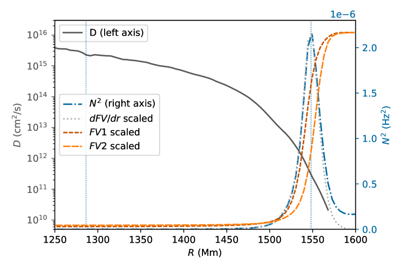
Figure 24: Diffusion coefficient $D$ from evolution of spherically averaged abundance profiles for heating factors $1000\times$ (M114, top) and $100\times$ (M116, bottom). $D$ is calculated according to the diffusion equation inversion method (§2.4). For M116 the two time average dump ranges are $[1050,2050]$ and $[3050,4050]$ respectively, and for M114 the averaging dump ranges are $[2725,3200]$ and $[3450,3925]$ respectively. Shown also is the Brunt-Väisälä frequency squared (blue dash-dotted) and the gradient of the fractional volume concentration (dotted grey lines, taken of the FV profile at the dump in the middle of the total range used for this analysis, which is dump $2550$ for M116 and 3325 for M114, and scaled so that the FV gradient and $N^{2}$ curve peaks match). The thin, blue-dotted vertical lines to the right indicate the radius of $N^{2}$-peak for which a power spectrum is shown in Fig. 16 and where $D_{\mathrm{IGW-hydro}}$ is measured. The left vertical lines are at the location $0.75\mathrm{H_{P0}}$ further inward, where the convective diffusion coefficient $D_{\mathrm{conv-hydro}}$ is measured. Also shown are the two fractional volume concentration profiles FV1 and FV2 (scaled to match the range on the right axis, $FV\in[0,1]$) at the first and last dump of the overall dump ranges used for the $D$ analysis.

Just as found previously (Müller et al., 2016; Jones et al., 2017; Andrassy et al., 2020), both convective velocity components follow the scaling $U_{\mathrm{conv}}\propto L^{1/3}$ (Fig. 26). The convective mixing coefficient follows the same scaling, consistent with the usual expression $D_{\mathrm{conv}}=\frac{1}{3}l_{\mathrm{mix}}v_{\mathrm{conv}}$ where $l_{\mathrm{mix}}$ is the mixing length. Since both $D_{\mathrm{conv-hydro}}$ and the convective velocities scale with the heating factor with the same power, then, assuming the above expression for $D_{\mathrm{conv}}$, the mixing length $l_{\mathrm{mix}}$ is independent of the heating factor. Fig. 27 shows

$$\alpha_{\mathrm{mix}}=\frac{1}{\mathrm{H_{P}}}l_{\mathrm{mix}}=\frac{3}{\mathrm{H_{P}}}\frac{D_{\mathrm{conv-hydro}}}{u}{}$$ (9)

for $u=U_{\mathrm{r}}$, the radial velocity component, and $u=U_{\mathrm{total}}=\sqrt{U_{\mathrm{r}}^{2}+U_{\mathrm{h}}^{2}}$, the total velocity magnitude.

The mixing-length parameter determined in this way increases from the convective boundary, where it is essentially zero, to order unity at almost one pressure scale height into the convective core, i.e. at about one pressure scale height into the convection from the Schwarzschild boundary $\alpha_{\mathrm{mix}}\approx 1$. A gradual increase of the mixing length from the boundary to well inside the convective core has previously been observed in hydrodynamic simulations of O-shell convection in a massive star by Jones et al. (2017, Eq.  (4)), who suggested that the mixing length parameter should be

$$\alpha_{1}=\min(\alpha_{\mathrm{mix}},\frac{|r-r_{\mathrm{SB}}|}{\mathrm{H_{P}}})\,.{}$$ (10)

adopting $\alpha_{\mathrm{mix}}=1$. $\alpha_{1}$ calculated in this way is shown in Fig. 27, and the slight bend reflects the radius dependence of $\mathrm{H_{P}}$. In these core-convection simulations, the mixing-length parameter is better modeled with an exponential

$$\delta r=\frac{|r-r_{\mathrm{SB}}|}{\mathrm{H_{P}}}\,,\ \alpha_{2}=\min(\alpha_{\mathrm{mix}},4e^{7(\delta r-1)}){}$$ (11)

again adopting $\alpha_{\mathrm{mix}}=1$. As shown in Fig. 27 this matches the mixing-length parameter profile determined from the simulations using the total velocity magnitude better.

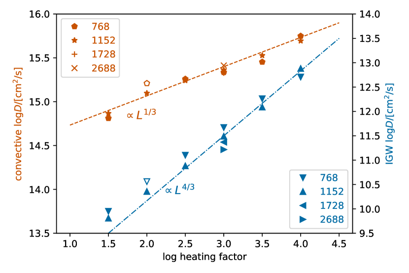
Figure 25: Scaling of diffusion coefficients determined by the diffusion equation inversion method (§2.4) as a function of heating factor. Hexagons, stars, plusses, and crosses represent convective diffusion coefficients $D_{\mathrm{conv-hydro}}$ taken at $0.75\mathrm{H_{P0}}$ below the $N^{2}$-peak radius (left axis). Triangles show the diffusion coefficients $D_{\mathrm{IGW-hydro}}$ at the $N^{2}$-peak radius as shown in Fig. 24. Two power laws shifted to be nearer to where the points are located are shown with dashed and dash-dotted lines.

The diffusion coefficient determined at the radius of the $N^{2}$-peak follows a scaling with heating factor $\propto L^{4/3}$ for heating factors $\geq 10^{2.5}$. This is distinctly different from the mixing scaling found for $D_{\mathrm{conv-hydro}}$ measured in the convective core and implies that the physical mixing process is fundamentally different from turbulent convection. This adds evidence to the expectation that mixing at the $N^{2}$-peak is caused by IGWs. In §5.3 we compare this mixing with predictions in terms of IGW-induced shear according to Eq. (6), and we turn therefore now to exploring the properties of vorticity in our simulations.

5.2 Vorticity scaling relations

Expression Eq. (6) relies on the assumption that the horizontal vorticity component is much larger than the radial vorticity component, so that $|\bm{\nabla\times}u|\approx|\bm{\nabla\times}u|_{\mathrm{h}}$. This is indeed expected for IGWs and borne out by our simulations, as shown in Fig. 28. The bottom panel shows the exact location of the $N^{2}$-peak in relation to the vorticity profile, as well as the Richardson number calculated from the vorticity as outlined in §2.4, using spline representations to find the precise vorticity at the radius of the $N^{2}$-peak. This shows that the local vorticity magnitude peak is $\approx 25\;\mathrm{\mathrm{M}\mathrm{m}}$ further inward relative to the $N^{2}$-peak, and that at that radius and above, the ratio of horizontal to vertical vorticity components exceeds $\approx 10$.

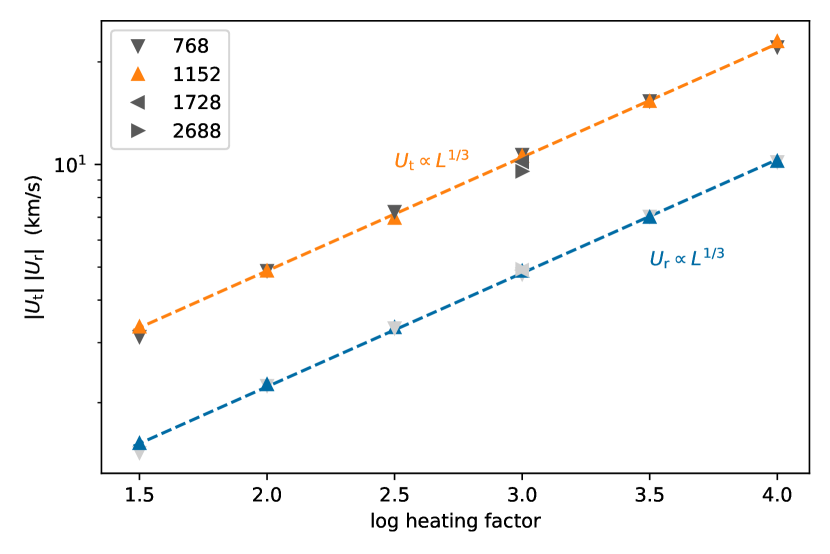
Figure 26: Horizontal and radial velocity magnitude in the convection zone at the same radius, $0.75\mathrm{H_{P0}}$ inward from the radius of the $N^{2}$-peak.

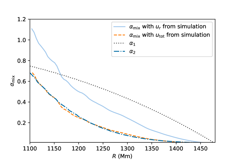
Figure 27: Mixing-length parameter $\alpha_{\mathrm{mix}}$ as a function of radius in the outer third of the convective core for simulation M116 ($100\times$ heating factor, $1152^{3}$-grid) using Eq. (9) with radial velocity component (blue solid) and total velocity magnitude (dashed orange) as well $\alpha_{1}$ according to Eq. (10) and $\alpha_{2}$ according to Eq. (11). See text for details.

The vorticity profiles for four different grid resolutions are shown in Fig. 29. The lower three grid resolutions are shown averaged over a time range after the convective boundary has migrated through the initial $N^{2}$-peak profile (Fig. 15). The idea was that we may avoid in this way a possible dependence of the vorticity profile on the shape of the $N^{2}$-peak profile. The highest resolution run was not followed to those late times. For this reason, the time ranges over which we average the three lower resolution runs and the highest resolution runs are not the same. In any case, in these simulations vorticity magnitude of IGWs in the stable layer shows no sign of convergence. At $N^{2}$-peak $|\bm{\nabla\times}u|^{2}$ scales $\propto N_{\mathrm{x}}^{2}$ (Fig. 30). The question of whether or not the IGW vorticity converges in the simulations will depend on the effect of radiative diffusion, which could dampen small-scale fluctuations. This question will therefore be revisited with simulations that include radiative diffusion and have reached a quasi-equilibrium.

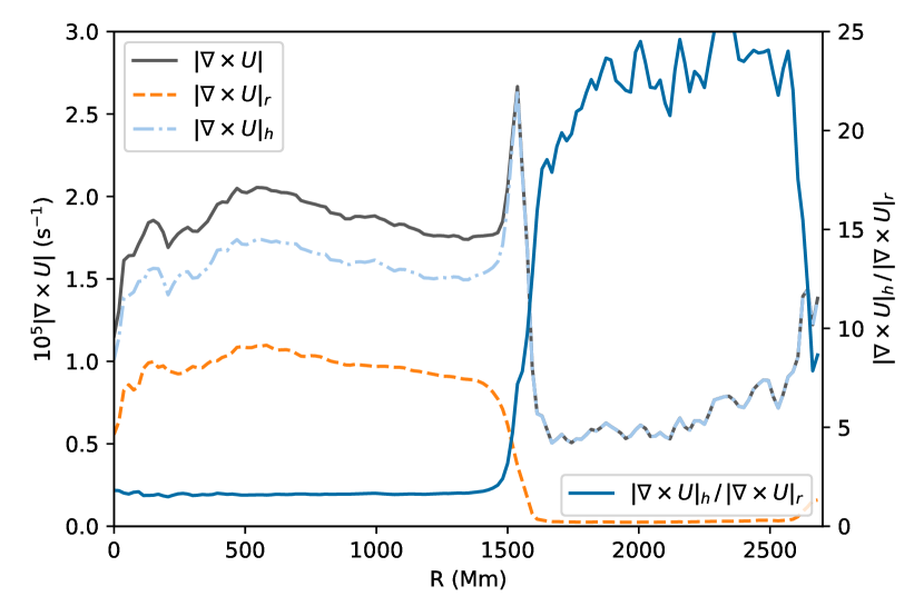
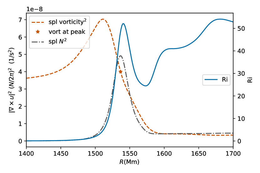
Figure 28: Top: Vorticity profile as well as the radial and horizontal components. Bottom: Profiles of $|\bm{\nabla\times}u|^{2}$, $N^{2}$, and the Richardson number $Ri\approx\frac{N^{2}}{|\bm{\nabla\times}u|^{2}}$ (cf. §2.4). The orange star indicates the radius of the $N^{2}$-peak. Both plots are for run M114 ($1152^{3}$ grid, $1000\times$ heating factor) at dump 4425 corresponding to time $3142\;\mathrm{\mathrm{h}}$.

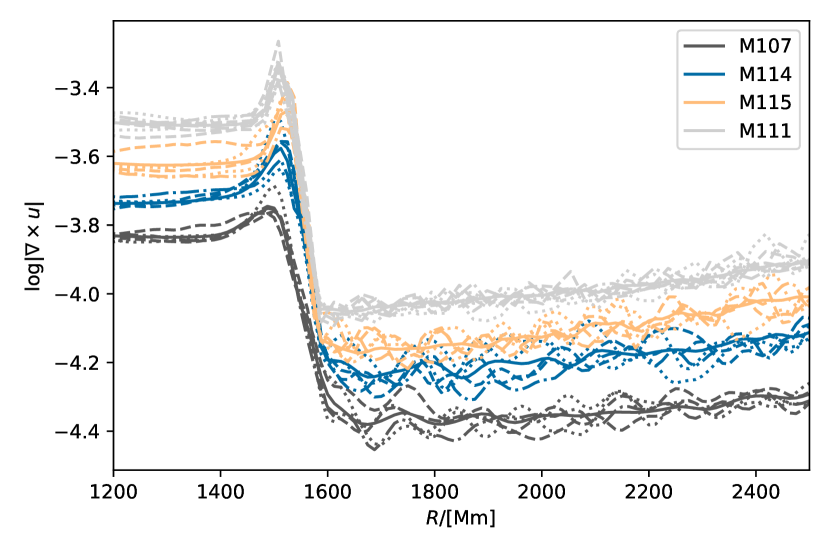
Figure 29: Spherically averaged vorticity profiles for $1000\times$ heating runs in M107 ($768^{3}$), M114 ($1152^{3}$), M115 ($1728^{3}$), and M111 ($2688^{3}$). Solid lines show the average of 442 dumps between $t=1349$ and $1662\;\mathrm{\mathrm{h}}$, except for M111, where 817 dumps in the time range $569$ to $1316\;\mathrm{\mathrm{h}}$ are averaged. The dashed, dotted, and dash-dotted lines show spherically averaged profiles for individual dumps in this time range every 100 dumps. The 3D vorticity data is calculated from the briquette data.

The analysis of the time evolution of vorticity shows fluctuations over long periods. The M107 time evolution of the average in the range $1900<R/\mathrm{M}\mathrm{m}<2100$ shows long-term $\approx 700\mathrm{h}$ variations with amplitudes of $\approx 10\%$.

Next we establish how vorticity scales with heating rate. The simulation vorticity in the convection zone displays the scaling relation $|\nabla\times U|\propto L^{1/3}$ (top panel Fig. 31). The spectrum represents the spatial scale distribution and therefore the denominator of the velocity gradient. The spectrum (Fig. 6) remains approximately the same as a function of heating, and thus the vorticity scaling follows the velocity scaling (§5.1).

The expected scaling of IGW vorticity with heating factor is based on the assumption that the kinetic energy flux of IGWs is proportional to the convective flux

$$F_{\mathrm{IGW}}=\mathcal{M}F_{\mathrm{conv}},$$

where $\mathcal{M}\propto v_{\mathrm{conv}}$ is the Mach number (e.g. Rogers et al., 2013). Given Eq. (7) and $v_{\mathrm{conv}}\propto L^{1/3}\propto F_{\mathrm{conv}}^{1/3}$, it follows that

$$U_{\mathrm{r}}\propto L^{2/3}$$

and

$$U_{\mathrm{t}}\propto L^{2/3}$$

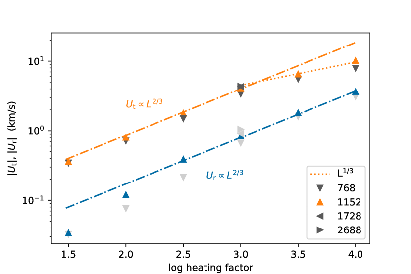
Figure 32: Tangential and radial velocity components at the $N^{2}$-peak radius as a function of heating factor. Upside-down triangles are from the $1152^{3}$-grid simulations. The lower sequence of blue and light grey symbols show the radial velocity component. Orange and dark grey symbols represent the tangential velocity component. Dash-dotted lines show scaling $\propto{2/3}$ and the dotted line shows scaling $\propto{1/3}$.

for fixed values of $n$ and $l$ and for the same stellar model. Our simulations are mostly consistent with this scaling. Fig. 32 shows the tangential and radial velocity component magnitudes at the radius of the $N^{2}$-peak. For the simulations with the lowest heating factors the grid resolution becomes insufficient and the radial velocity component values drop below the scaling relation. Note how the $768^{3}$-grid simulations drop more than those with $1152^{3}$ grid. The scaling relation for these velocities one pressure scale height $\mathrm{H_{P0}}$ further out in the envelope looks the same, except with tangential velocities roughly a factor of two smaller (Figs. 8 and 7). However, at both locations, the tangential velocity component deviates from the scaling relation for IGWs derived above to follow $\propto L^{1/3}$ for heating factors $>1000$.

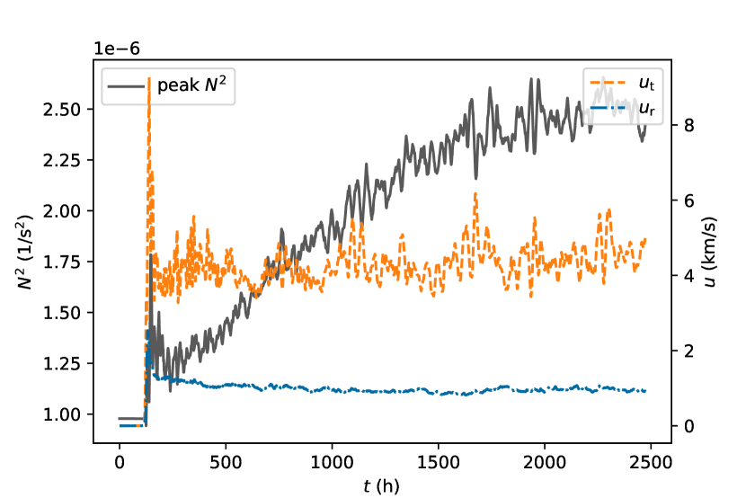
Figure 33: Tangential and radial velocity magnitude at the radius of the $N^{2}$-peak for run M115 ($1728$ grid, $1000\times$ heating factor) and the value of $N^{2}$ at the radius of the $N^{2}$-peak. $N^{2}$ gradually increases over the first $1500\;\mathrm{\mathrm{h}}$ while the boundary migrates outward through the initial boundary profile (cf. §4.1 and middle panel Fig. 15).

One may think that this break from the scaling relation by the tangential velocity component is due to lower heating factor runs retaining most of their original $N^{2}$-peak profiles, while velocities for higher heating factor runs have been measured at later times, when the boundary has migrated through the initial $N^{2}$-peak profile as discussed previously in §4.1. If this were the case, we would see variation in the tangential velocity component during the initial $1500\;\mathrm{\mathrm{h}}$ as the convective boundary migrates through the initial $N^{2}$-peak profile in a $1000\times$ heating run. Fig. 33 shows that this is not the case. Immediately after the initial $\approx 100\;\mathrm{\mathrm{h}}$ (about a convective turn-over time), when the first convective plumes reach the boundary, the horizontal velocity magnitude reaches its steady-state value. During the initial $\approx 1500\;\mathrm{\mathrm{h}}$, the maximum $N^{2}$ value gradually increases, signaling the continued change of the profile. After this time, the $N^{2}$ max remains constant, corresponding to the phase of self-similar migration of the boundary. During this entire time, the tangential velocity magnitude remains constant, demonstrating that it does not depend on the shape of the $N^{2}$-peak.

Instead, a different explanation of the break from the tangential velocity scaling relation is more plausible. The velocities of IGWs scale with twice the power the convective velocities scale with. At some heating factor the IGW velocities would exceed the convective velocities. For heating factor $10^{4}\times$, the tangential velocity according to the scaling law would be $18.6\;\mathrm{\mathrm{k}\mathrm{m}\sec^{-1}}$ at the $N^{2}$-peak  whereas the convective tangential velocity component at $0.75\mathrm{H_{P0}}$ further inward is $22.6\;\mathrm{\mathrm{k}\mathrm{m}\sec^{-1}}$. Since IGW motions are excited by convective motions in the core it makes sense that at some point the IGW velocities cannot continue to follow their steep power law, but instead will follow the shallower power law of the convective motions.

For heating rates $\leq 100\times$ for an $1152^{3}$ grid and $\leq 316\times$ for a $752^{3}$ grid, $\mathcal{M}$ numbers become too low for the given grid resolution to resolve the flow velocities accurately (see Andrassy et al., 2020, for same effect in O-shell convection simulations, Fig.  15) which shows first in the smaller $U_{\mathrm{r}}$ component.

Again, since the IGW spectrum does not depend much on the heating factor, especially at high wave numbers (Fig. 19) the IGW vorticity follows the same scaling $|\nabla\times U|\propto L^{2/3}$ as the velocity. The IGW vorticity data in the radiative envelope from our simulations is consistent with this scaling for heating factors in the range $100$ to $1000$ (Fig. 31) for both the envelope and the $N^{2}$-peak radius. Extra care has been taken in view of the steep vorticity gradient at $N^{2}$-peak to retrieve the values from spline interpolations (bottom panel, Fig. 28). Fig. 31 shows the vorticity scaling for both the envelope (orange symbols in top panel) and for the $N^{2}$-peak (bottom panel).

The simulation vorticity follows the scaling pattern of the tangential velocity component $\propto L^{2/3}$ for heating factors $<1000$ and $\propto L^{1/3}$ for larger heating factors. Since the vorticity magnitude for IGWs is essentially the horizontal vorticity component (Fig. 28), this implies that the total vorticity magnitude is dominated by the term $\partial U_{\mathrm{h}}/\partial r$ in Eq. (5), and it confirms that the simulated IGW vorticity magnitude represents dominantly horizontal shear motions.

The $768^{3}$-grid simulations generally fall below the scaling $L^{2/3}$, and the change to $1/3$ scaling is not as clear as it is in the $1152^{3}$-grid simulations. This is especially so for the lowest heating factor, where also the $1152^{3}$-grid vorticity falls below the $L^{2/3}$ scaling. This effect can be attributed to insufficient grid resolution at the lowest $\mathcal{M}$ numbers. Since the tangential velocity component does trace the $2/3$ power law down to the lowest heating factors, it is likely that at these low heating rates, the radial resolution of horizontal flow features is insufficient to capture the smaller scales, hence the calculated velocity gradients are too small.

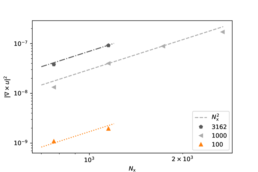
Figure 30: $|\bm{\nabla\times}u|^{2}$ at $N^{2}$-peak radius as a function of grid resolution. $N_{\mathrm{x}}$ is the number of grid cells in one dimension. The legend gives the heating factor.

The peak of the $U_{\mathrm{r}}$ spectra is somewhat lower for the highest and lowest heating rates. However, for the lowest heating rate the deviation of spherically- and time-averaged radial velocities from the scaling laws established by the higher heating-rate runs (§5.2) suggests that the lowest heating rate case shown (M116) has insufficient grid resolution at $1152^{3}$ grids to resolve the $U_{\mathrm{r}}$ velocity component accurately. Saux et al. (2022) suggested that higher heating rates with their larger convective frequencies would excite IGWs with higher frequencies. There is no evidence for that in these spectra at the $N^{2}$-peak location. However, if such differences appear only near the convective frequency then higher frequency resolution, i.e. longer time series than available from these simulations may be required to detect such trend if it exists.

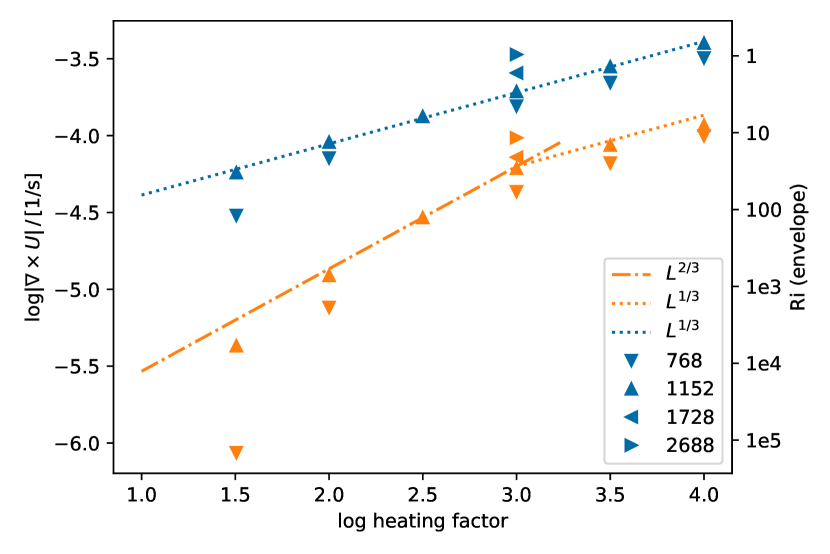
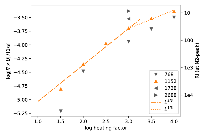
Figure 31: Vorticity as a function of heating. Top: envelope (orange) and convection (blue); bottom: at $N^{2}$-peak radius. The vorticity values for the envelope are obtained by time-averaging the spherical averages (Fig. 29) over the range $R/\mathrm{M}\mathrm{m}\in[1800,2000]$. The convective vorticity values are the radial average over the range $800<R/\mathrm{M}\mathrm{m}<1100$. On the right ordinate, the Richardson number according to Eq. (3) is shown. Strictly speaking, each point would have its own value of $N^{2}$, and points can’t simultaneously be on the same vorticity scale and on the same Ri scale. Here, the Ri axis is indicative, assuming for all points the average value for $N^{2}$ at the $N^{2}$-peak of all $1152^{3}$-grid simulations ($<N^{2}>=1.5\times 10^{-6}\;\mathrm{\mathrm{1/s^{2}}}$ , $N^{2}\in[1.1,1.9]10^{-6}\mathrm{1/s^{2}}$).

5.3 Critical interpretation of measured IGW mixing as shear-mixing

In this section, we discuss the scaling relations from the simulations for IGW mixing and vorticity under the assumption that IGW mixing is due to shear mixing as described in §2.4, specifically Eq. (6). We thereby test whether, based on the simulations presented here, we are able to confirm or rule out that this is the case.

5.3.1 Scaling of $D_{\mathrm{IGW-hydro}}$ with $1/Ri$

Fig. 25 shows that, focusing on the $1152^{3}$-grid simulations, the measured $D_{\mathrm{IGW-hydro}}$ mixing coefficients follow the scaling $\propto L^{4/3}$ for $\log\mathrm{heating\ factors}\goa 2$. This would be consistent with the shear-mixing model Eq. (6) with IGW vorticity scaling with $L^{2/3}$. However, $|\bm{\nabla\times}u|\propto L^{1/3}$ and not $\propto L^{2/3}$ for heating factors $\geq 1000\times$, yet $D_{\mathrm{IGW-hydro}}$ does not follow this power-law change toward a slower increase with heating. Again, as in the previous section, we consider if this behaviour could be due to the somewhat different $N^{2}$-peak profiles for lower heating rate runs versus the higher heating rate runs. The possible effect of the $N^{2}$ dependence in Eq. (6) can be eliminated by establishing the scaling relation of $D_{\mathrm{IGW-hydro}}$ with $1/Ri$:

$$D_{\mathrm{IGW-hydro}}\propto\frac{1}{Ri}\approx\frac{(\nabla\times\mathbf{u})^{2}}{N^{2}}\propto L^{4/3}\,.{}$$ (12)

If IGW mixing is due to shear mixing following Eq. (6), then we should find $D_{\mathrm{IGW-hydro}}\propto\frac{1}{Ri}$ for all heating factors. However, as shown in Fig. 34, this is not the case. Focusing again on the higher accuracy $1152^{3}$-grid simulations, the scaling follows the trend expected for shear mixing for heating factors $<1000\times$. But for larger heating factors, the scaling power changes by a factor of two, consistent with the change of vorticity scaling being the dominant aspect. Thus, the small variation of $N^{2}$ as a function of heating is not responsible for the change of scaling at heating factors $\geq 1000\times$. To make this point even clearer, we show each pair of ($1/Ri$, $D_{\mathrm{IGW-hydro}}$) in Fig. 34 using both the actual $N^{2}$ value measured for each simulation (filled symbols), as well as the $1/Ri$ values resulting from using an average, constant value for $N^{2}$ (open symbols). This shows that while individual points may shift a bit, the break from the scaling in Eq. (12) does not depend on the minor dependence of $N^{2}$ on the heating factor.

The change of scaling in Fig. 34 seems to be in contradiction to the hypothesis that the measured IGW mixing is due to shear mixing according to Eq. (12). Even though the vorticities do not follow the scaling law expected for IGWs for heating factors $>1000\times$ because the tangential velocity does not follow the IGW scaling relation in those cases (§5.2), we may still expect Eq. (12) to hold. But this is not the case, as the break from scaling in the relation of $D_{\mathrm{IGW-hydro}}$ with $1/Ri$ (Fig. 34) shows. A complicating factor could be that Eq. (6) also contains the thermal conductivity, which will be discussed in the next section.

The $768^{3}$-grid simulations follow the scaling $D_{\mathrm{IGW-hydro}}\propto 1/Ri$ for all but the lowest heating factor. However, as pointed out before, $768^{3}$-grid vorticities less accurately follow the $L^{2/3}$ IGW vorticity scaling and therefore do not exhibit the change in scaling from power $2/3$ to $1/3$ as clearly. For the lowest heating factors, mixing is larger compared to the $L^{4/3}$ scaling (Fig. 25), and more so for smaller grids. This is consistent with numerical diffusion contributions, to be discussed further below.

A question arises as to how sensitive the determination of $D$ and $1/Ri$ is to the exact position of where the values are taken (cf. Fig. 28). Mini-profiles provided for runs M114 and M116 as short solid lines in Fig. 34 show the simultaneous change of both quantities accrosss the $N^{2}$-peak feature. For each of these lines, the large $1/Ri$ end of the line corresponds to the inside of the $N^{2}$-peak profile, and this is the convection side. For the broader M116 peak, the mini-profile is approximately aligned with the $\propto 1/Ri$ scaling law. The M114 mini-profile follows the heating-series scaling relation broadly but deviates on the stable side of the $N^{2}$-peak profile.

5.3.2 Thermal conduction

These simulations do not include thermal conduction. However, the shear-mixing model described in §2.4 requires that $D_{\mathrm{IGW-hydro}}\propto$ the thermal diffusivity $K$ (Eq. (2)). As discussed in §2.4, thermal loss of entropy memory enables shear flows to cause mixing for $Ri>1/4$. Without thermal conduction, displaced fluid elements would remember the entropy of their origin and return ultimately to that radial position. Thus, thermal conduction would facilitate partial or complete entropy memory loss without which mixing according to the shear mixing mechanism outlined in §2.4 would be impossible. Since these simulations do not include thermal conduction explicitly, numerical diffusion of entropy would be facilitating IGW mixing if it is caused by shear according to Eq. (2). The numerical entropy diffusion would be related to the accuracy of PPM used to calculate the hydrodynamics, with error terms expected to scale with the number of grid points (in one dimension) $N_{\mathrm{x}}$ as $N_{\mathrm{x}}^{-3}$ (Porter & Woodward, 1994). However, the advection of concentration $FV$ is done in PPMstar with the higher-order PPB method. Due to this feature of PPMstar treating hydrodynamic and concentration advection at different orders, these simulations could capture mixing due to small-scale shear at $Ri>1/4$ calculated with high-order PPB aided by thermal conduction due to more efficient entropy diffusion resulting from the lower order of PPM.

More specifically, in the presence of fluid shear the PPM difference scheme has an effective numerical viscosity that has been measured and characterized quantitatively in Porter & Woodward (1994). This viscosity arises from interpolation errors that cause a slight diffusion of mometum. The diffusion of entropy in such a flow should occur through the same sort of interpolation errors and thus should be characterized in the same way in terms not of effective viscosity but instead of effective thermal diffusivity. The effective viscosity of the PPM scheme in this context consists of two terms, one that scales as $\Delta x^{3}/\lambda^{2}$ and another scaling as $\Delta x^{4}/\lambda^{3}$ where $\Delta x$ is the cell width. The second term becomes important only for sinusoidal disturbance wavelengths, $\lambda$, that are smaller than about $10\Delta x$. For reasonably resolved wavelengths $\lambda$ the dominant term in the effective viscosity of the PPM scheme scales as $\Delta x^{3}/\lambda^{2}$. This means that for a given grid cell size $\Delta x$ the effective viscosity is inversely proportional to the square of the disturbance wavelength. Consequently, there is no single viscosity that one can ascribe to a PPM simulation on a given grid, because the effective viscosity rapidly becomes smaller as the wavelength of the disturbance of interest increases. In the flows discussed here, we consider shear generated by IGWs in the region of $N^{2}$-peak at the convective boundary. If we consider grids that all capture the spectrum of such IGWs fairly well, then we would expect the resulting diffusion of entropy to scale with $\Delta x^{3}$. If, instead, more of the IGW spectrum at shorter wavelengths is captured as the grid is refined, and if this newly captured spectrum component contains sufficient power to be important in diffusing entropy, then the effective entropy or species diffusion could scale differently with $\Delta x$. As shown in the left column of Fig. 19 the overall spectrum is captured fairly well by all grids, but it is also correct that more power appears at higher wave numbers.

In PPMstar species advection is followed with the higher-order PPB scheme (Woodward et al., 2015) whereas the hydro is computed using PPM. Formally, PPB is two orders more accurate than PPM, so its numerical diffusion should scale with grid resolution not as $\Delta x^{3}$ but as $\Delta x^{5}$. Ultimately, an advection scheme can capture species flows in absolute terms only as accurately as the underlying velocity field. In the bottom panel of Fig. 24, it can be seen that the FV gradient profile differs slightly from the $N^{2}$ profile. In a hypothetical simulation without physical heat conduction in which the numerical species and entropy diffusion are the same, initially identical $FV$ (concentration) and entropy profiles must remain identical with time everywhere in the simulation. In the bottom panel of Fig. 24 it can be seen that the $FV$ gradient profile is slightly different from the $N^{2}$ profile. Despite not including thermal diffusivity in these simulations, numerical diffusion of heat changes the entropy profile in addition to dynamic process, which for concentration mixing are followed with the higher accuracy of the PPB scheme. This is an indication that in these simulations species mixing and entropy mixing are indeed subject to different numerical accuracy.

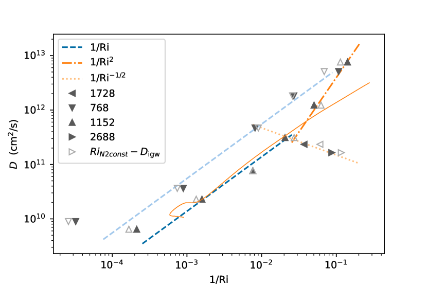
Figure 34: IGW mixing diffusion coefficient at the $N^{2}$-peak radius as in Fig. 25 as a function of $1/Ri=\frac{|\bm{\nabla\times}u|^{2}}{N^{2}}$. In order to show the magnitude of the variation of $N^{2}$, open symbols show $1/Ri$ values calculated with the $N^{2}$ average of the $1152^{3}$-grid simulations (see caption of Fig. 31). A thin solid orange line provides the relation between $D$ and $1/Ri$ along the $N^{2}$-peak profile for M116 (Fig. 24) for the radius range $R\in[1465,1555]\;\mathrm{\mathrm{M}\mathrm{m}}$, where values of large $1/Ri$ correspond to small radii.

$D_{\mathrm{IGW-hydro}}$ is the measurement of species transport determined from the time evolution of $FV$ profiles of the simulations (§5.1). Fig. 34 shows that $D_{\mathrm{IGW-hydro}}\propto(1/Ri)^{-1/2}$ as a function of grid resolution for heating factor $1000$. This suggests to analyze the dependence of the species and entropy diffusivity on grid resolution a bit further. Fig. 35 shows that $D_{\mathrm{IGW-hydro}}\propto N_{\mathrm{x}}^{-1}$, where $N_{\mathrm{x}}$ is the number of grid points in one direction. This would be consistent with the case of numerical diffusivity proportional to $\Delta x$ mentioned above. $N^{2}$ does not depend significantly on $N_{\mathrm{x}}$. However, $|\bm{\nabla\times}u|^{2}\propto N_{\mathrm{x}}^{2}$ (Fig. 30), and if IGW mixing is due to shear according to Eq. (6) the scaling of $D_{\mathrm{IGW-hydro}}$ with grid resolution can also be understood as a consequence of numerical entropy diffusion scaling with $N_{\mathrm{x}}^{-3}$. Using the measured $D_{\mathrm{IGW-hydro}}$ and $|\bm{\nabla\times}u|$  a hydrodynamic IGW diffusivity can be determined according to

$$K_{\mathrm{hydro}}=\frac{D_{\mathrm{hydro}}{N^{2}}}{\eta(\nabla\times\mathbf{u})^{2}}\,.{}$$ (13)

This would be a reflection of the numerical PPM entropy diffusivity if the measured $D_{\mathrm{IGW-hydro}}$ is due to shear mixing according to Eq. (6), and using $\eta=1$. Then the scaling for $K_{\mathrm{hydro}}$ with $N_{\mathrm{x}}$ follows from that of vorticity and $D_{\mathrm{IGW-hydro}}$ and is $\propto N_{\mathrm{x}}^{-1}/N_{\mathrm{x}}^{2}=N_{\mathrm{x}}^{-3}$ as shown in Fig. 36. This corresponds to the expected scaling of the PPM error terms if all grids resolve the relevant scales reasonably well (Porter & Woodward, 1994).

$K_{\mathrm{hydro}}$ is a possible expression of the entropy diffusion in the sense that if IGW mixing is due to shear mixing according to Eq. (6), then the PPM entropy diffusion has the same cumulative effect on entropy memory loss of perturbed fluid elements that a thermal diffusivity of this magnitude would have, given the measured mixing, the vorticity and $N^{2}$ of the simulation. However, as explained earlier in this section numerical entropy diffusivity has a very different dependence on the spatial spectrum than radiative diffusion would have. Therefore, the values and scaling relations determined for $K_{\mathrm{hydro}}$ are specific to the particular setup and are not numerically equal to a numerical viscosity. With these caveats in mind, we can then ask what the grid size would be so that for a given simulation of this setup, the effect of thermal conductivity $K$ is approximately as large as the measured $K_{\mathrm{hydro}}$. In order to maintain the same thermal equilibrium stratification, $K$ would be added $\propto L$ in simulations with radiative diffusion. The $K$ values according to this scaling have been added as horizontal dotted lines for three heating factors to Fig. 36. Assuming $\eta=1$ simulations with $N_{\mathrm{x}}\goa 1400$ would satisfy $K_{\mathrm{hydro}}\loa K$ for $1000\times$ heating factors. At this or finer grids, a physical diffusivity scaled proportionally to the heating factor would dominate over numerical entropy mixing in its impact on IGW mixing if that mixing is due to shear mixing. Thermal diffusivity would have a number of other effects on the dynamic evolution of the overall simulation, for example in establishing the quasi-equilibrium state. The grid dependence of those effects would be different for numerical entropy diffusion compared to thermal diffusion.

Using a larger heating rate would in principle require a smaller $N_{\mathrm{x}}$, except that the measured mixing does not follow the shear mixing scaling in that case, thus making application of Eq. (13) questionable.

Considering the complex nature of the flow under consideration this analysis of cumulative effects of different types of error terms in the framework of a specific physics model may necessarily remain somewhat inconclusive. However, having established the dependencies of various quantities related to cause and effect of IGW mixing on grid resolution in these simulations without thermal conduction provides a valuable reference point for simulations that do include thermal diffusion.

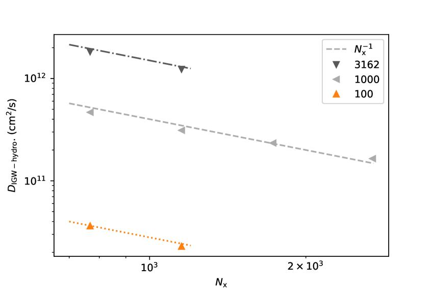
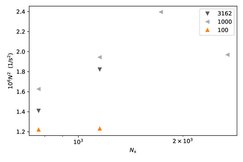
Figure 35: Top: $D_{\mathrm{IGW-hydro}}$ at $N^{2}$-peak radius as a function of grid resolution. $N_{\mathrm{x}}$ is the number of grid cells in one dimension. A power law with exponent $-1$ is also shown. The power law fit gives an exponent $-0.85$. Bottom: $N^{2}$ at peak. The lower $N^{2}$ for the $2688^{3}$-grid $1000\times$ run (M111) is due to the shorter duration of that run, in which the initial $N^{2}$-peak profile still dominates over the dumps averaged (cf. Fig. 33).

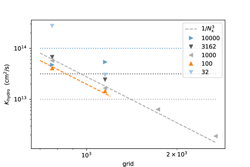
Figure 36: IGW effective entropy diffusivity in terms of $K_{\mathrm{hydro}}$ calculated from Eq. (13) under the assumption that measured IGW mixing is due to shear mixing, and using the simulation values $D_{\mathrm{IGW-hydro}}$  $|\bm{\nabla\times}u|$ shown in Fig. 35, and $\eta=1$. Dotted horizontal lines indicate the radiative diffusivity when scaled as $K\propto L$, from bottom to top for heating factors $1000\times$, $3162\times$, $10000\times$.

5.4 Discussion

The main results and findings of this section are as follows:

• We measured convective mixing and mixing due to IGWs for heating factors from $31.6\times$ to $10,000\times$, for at least two grid resolutions in each case, and for four grid resolutions for heating factor $1000\times$. These two sets of mixing coefficients follow distinctly different scaling relations $D_{\mathrm{conv-hydro}}\propto L^{1/3}$ and $D_{\mathrm{IGW-hydro}}\propto L^{4/3}$. This confirms their distinctly different underlying mixing physics.

• The convective mixing results are consistent with the commonly adopted relation $D_{\mathrm{conv-hydro}}\propto l_{\mathrm{mix}}v_{\mathrm{conv}}$. Our simulations support a new exponential model (Eq. (11)) of how the mixing-length parameter decreases toward the convective boundary of main-sequence core convection in a massive star. This mixing-length parameter can be used to relate the MLT convective velocity to the species-mixing diffusion coefficient, instead of using a constant MLT mixing-length parameter throughout the entire convection zone.

• We probe to what extent the measured IGW mixing is consistent with the predictions of shear-induced mixing (§2.4, Eq. (6)). The total vorticity magnitude of IGWs is dominated by the horizontal component, which in turn is dominated by the derivative of the horizontal velocity component in the radial direction. It follows a scaling law $|\bm{\nabla\times}u|^{2}\propto L^{4/3}$ for heating rates up to $1000\times$, but $\propto L^{2/3}$ above, likely because the higher power of IGW velocity scaling relative to convective velocity scaling leads to IGW velocities approaching those of the convective core. No matter what the cause of this change in scaling the measured $D_{\mathrm{IGW-hydro}}$ values should remain $\propto 1/Ri\propto|\bm{\nabla\times}u|^{2}$ according to the shear-mixing prediction of IGWs, which they do not (Fig. 34). This finding questions the interpretation of IGW mixing measured in these simulations as due to shear mixing according to Eq. (6).

• In these simulations without radiative conduction, the role of $K$ in Eq. (6) would be that of numerical entropy diffusion, which can be expressed as an equivalent $K_{\mathrm{hydro}}$ (Eq. (13)). This inferred diffusivity follows the scaling as a function of grid resolution that is consistent with the expected PPM error term if the relevant spectrum of IGWs is reasonably resolved on all grids.

This leads to the question of what can be concluded about the IGW mixing at nominal heating in a real star. By conducting a grid of simulations as a function of heating factor and grid resolution we have measured mixing due to IGWs in the $N^{2}$-peak region. The measured scaling for $D_{\mathrm{IGW-hydro}}\propto L^{4/3}$ does not explicitly take into account the expected dependence on $K$. If we use the scaling relation as it derives from the simulations (Fig. 25), then extrapolating the $1000\times$ measured $D_{\mathrm{IGW-hydro}}$ values to nominal heating yields $D_{\mathrm{IGW}}\approx 2.5\times 10^{7}\;\mathrm{cm^{2}/s}$. Such a large IGW mixing value would lead to significant changes of the evolution of a $25\;\mathrm{\mathrm{M}_{\odot}}$ star, in the Hertzsprung-Russell diagram and in terms of internal mixing that would lead to surface enrichment of He and CNO elements.

However, if we assume that IGW mixing is due to thermally-enhanced shear-mixing according to Eq. (6) (adopting for this estimate $\eta=1$), we can arrive at an estimate in the following way. The dependence of $K_{\mathrm{hydro}}$ on the heating factor is rather small (Fig. 36). We tentatively interpret Fig. 36 to suggest that a simulation with a heating factor of $1000\times$ and a grid size $N_{\mathrm{x}}$ somewhere between the $1152^{3}$ and $1728^{3}$ grid would be equivalent to a simulation with a radiative diffusivity $K$ that has been scaled $\propto L$, because at that $N_{\mathrm{x}}$ the inferred $K_{\mathrm{hydro}}$ is approximately the same as would be the scaled radiative diffusivity. A simulation with such a $N_{\mathrm{x}}$ therefore mimics a simulation with radiative diffusion included at the scaled rate. Then, interpolating between the measured diffusivities of the $1152^{3}$- (M114) and $1728^{3}$-grid (M115) runs, the resulting IGW diffusivity at $1000\times$ heating factor would be $\approx 3\times 10^{11}\;\mathrm{cm^{2}/s}$. Adopting from §5.2 that $|\bm{\nabla\times}u|^{2}\propto L^{4/3}$ and that $N^{2}$ does not contribute significantly to the scaling of $D_{\mathrm{IGW-thermal}}$, and considering that we assumed $K\propto L$, the scaling for IGW shear mixing would be $D_{\mathrm{IGW-thermal}}\propto L^{7/3}$ and $3\times 10^{11}\;\mathrm{cm^{2}/s}$ at $1000\times$ heating factor would correspond to $\approx 3\times 10^{4}\;\mathrm{cm^{2}/s}$ at nominal heating. This would be an upper limit, since it is possible that $\eta<1$.

Alternatively, scaling $Ri\approx N^{2}/|\bm{\nabla\times}u|^{2}\approx 50$ at $N^{2}$-peak (Fig. 28) using $|\bm{\nabla\times}u|^{2}\propto L^{4/3}$ and adopting for the nominal thermal diffusivity $K\approx 10^{10}\;\mathrm{cm^{2}/s}$, the estimate for IGW diffusivity is $D_{\mathrm{IGW}}\approx K/Ri=2\times 10^{4}\;\mathrm{cm^{2}/s}$, again adopting $\eta=1$. Such a low value would have a limited and local effect on mixing in the boundary region immediately above the convection-dominated core but would not contribute to mixing from the core to the surface over the main-sequence lifetime of a $25\;\mathrm{\mathrm{M}_{\odot}}$ star.

6 Conclusions

Our $4\pi$ 3D simulations include the entire convective core and an additional $\approx 1000\;\mathrm{Mm}$ in radius of stably stratified star above the convective core, amounting in combination to $\approx 50\%$ of the radial extent of a H-burning $25\mathrm{M}_{\odot}$ star. Convective flows are large-scale, and the largest coherent structure is a drifting dipole in which flows are passing through the centre to the convective boundary and returning along the boundary to the antipode. There, mutually opposing horizontal pressure gradients of the converging flow force the flow inward and create highly unstable boundary-separation wedges.

It is interesting to compare these results with the picture of convection on which MLT is based. The convection zone contains radially just over two pressure-scale heights. The notion of a dominant fluid element descending for a distance of about a mixing length toward the centre, and fluid elements rising from the centre to the boundary, can indeed be observed in the 3D simulations. But in the simulations, these same fluid flow elements simply stream right through the centre and do not turn around there. Our simulations show instead large-scale flows that flow directly through the central region but that do not originate nor terminate there, as in a flower petal pattern.

The power spectrum shows the familiar turbulent cascade in the inner regions but the spectrum of the radial velocity component flattens toward the boundary, while the spatial spectrum of the tangential velocity component remains close to $\propto l^{-5/3}$. Interactions of a broad spectrum of equally powerful convective motions excite IGWs in the stable layer. These IGWs display eigenmodes in good agreement with the predictions of GYRE models based on the spherically averaged radial structure of the 3D simulations. The transition from convective-dominated to wave-dominated flows can be characterized from the 3D data through the higher-order moments of the PDF of the radial velocity on the sphere of a given radius. The product of the skew and excess kurtosis has a maximum at the dynamic boundary, and for IGWs the PDF is Gaussian.

Our simulations show an unrealistically high mass-entrainment rate, similar to previous simulations (Meakin & Arnett, 2007; Gilet et al., 2013). The reason for these high entrainment rates is that the underlying MESA model, from which the initial setup for the 3D simulation is derived, is not in dynamic-thermal equilibrium (Anders et al., 2022). Simulations with radiative diffusion included, and with a sufficiently large nearly-adiabatic penetration zone, show a realistic mass-entrainment rate and will be presented in a forthcoming paper.

In §5, we showed that we measure mixing due to IGWs in the $N^{2}$-peak region. In order to determine IGW mixing at nominal heating, it is essential to identify the actual physical mechanism of IGW mixing in order to apply the correct scaling relation. In this paper, we have explored the shear-mixing model to this end (§2.4). The simulations presented here do not provide conclusive evidence for this physical mixing process. If IGW mixing is due to shear, as described by Eq. (6), then the simulations presented in this paper suggest that $D_{\mathrm{IGW}}\approx 2$ to $3\times 10^{4}\;\mathrm{cm^{2}/s}$ in the $N^{2}$-peak region above the convective core. Such mixing rates would at most have local impact on mixing but would not lead to mixing that alters the surface composition in a $25\;\mathrm{\mathrm{M}_{\odot}}$ star over the main-sequence lifetime. However, other physical mixing mechanisms are possibly responsible for IGW mixing. For example, in a forthcoming paper, we will explore a process that we call advective stochastic mixing (ASM), which would scale as $D_{\mathrm{IGW}}\propto U_{\mathrm{r}}^{2}/N$ and may depend less or not at all on thermal diffusivity. This model would also be compatible with the scaling relations established here but would lead to larger IGW mixing efficiencies when extrapolated to nominal heating.

Data availability

3D and spherically averaged 1D simulation outputs are available at https://www.ppmstar.org along with python notebooks that have been used to create plots in this paper.

Appendix A Constructing the 1D base state

In order to construct the base state from a MESA profile, the entropy and pressure is calculated from the MESA temperature, density, and mean molecular weight profiles.

$$P_{\mathrm{gas}} = \frac{\mathcal{R}}{\mu}\rho T$$ (14)

$$S_{\mathrm{gas}} = c_{V}\log T-\frac{\mathcal{R}}{\mu}\log\rho+\mathrm{const.}{}$$ (15)

With a maximum radius of $R_{\mathrm{max}}=2700\mathrm{M}\mathrm{m}$, for these simulations a grid cell is $\Delta x=7.03\mathrm{M}\mathrm{m}$ on a $768^{3}$-grid. This is usually the smallest grid used in our simulations. The following filtering procedure is performed on a ten times finer radial grid. The entropy on this filtering grid is obtained by interpolating the entropy calculated with Eq. (15) from the MESA $T$, $\rho$, and $\mu$ using scipy.interpolate.PchipInterpolator.

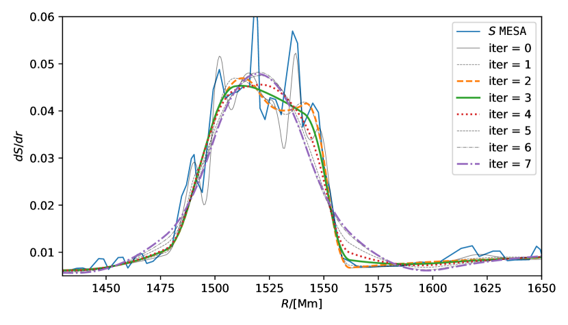
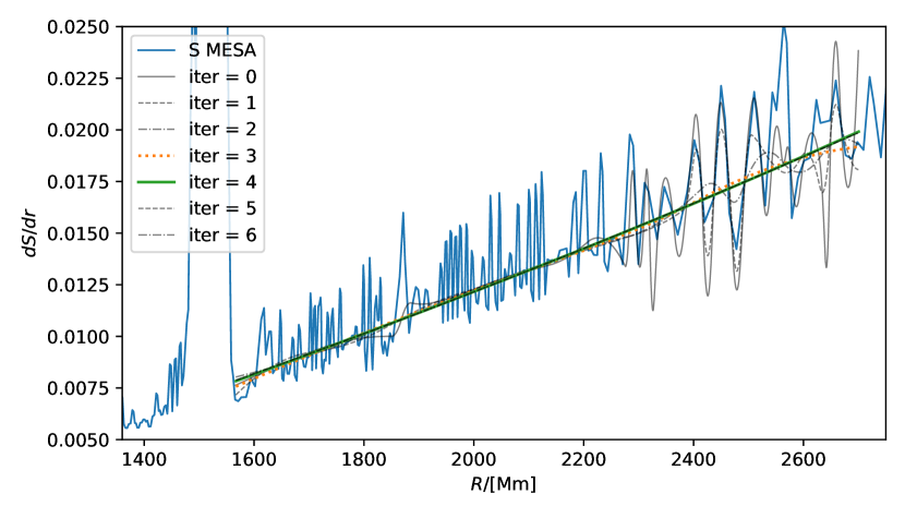
Figure 37: Filtering of MESA radial entropy derivative through recursive spline fitting, done separately for the core-envelope transition (top) and the envelope (bottom).

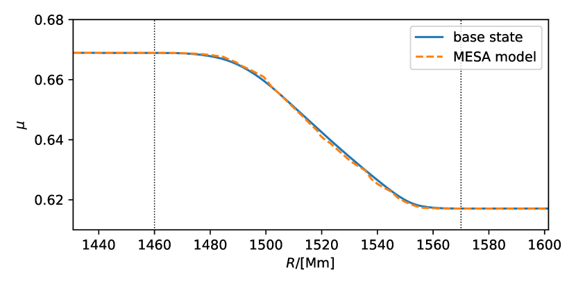
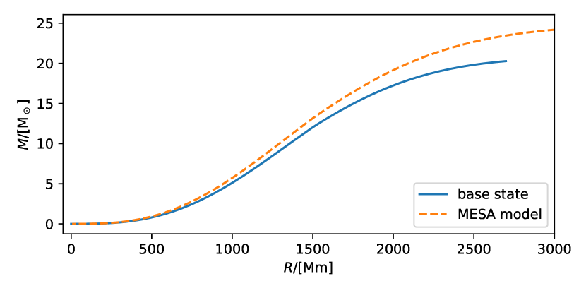
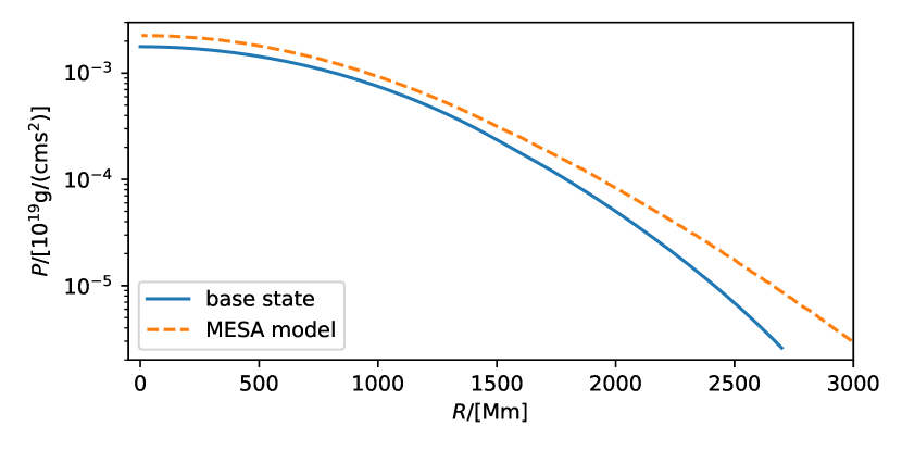
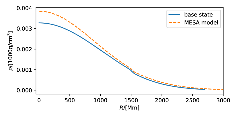
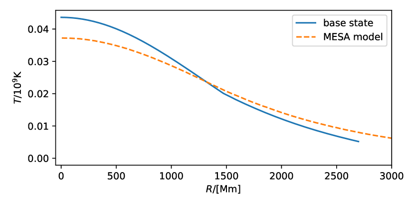
Figure 38: Comparison of adopted base state for the 3D simulations and the MESA radial profile. From top to bottom: mean molecular weight, mass, pressure, density, temperature. Except for mass, quantities are given in their code units.

In order to remove short wavelength noise in the radial MESA profile and obtain profiles with smooth first derivatives and continuous second derivatives, we have tried a number of strategies to filter the MESA entropy profile, including moving averages with different filter width, fitting the boundary with up to three Gaussians, or fitting with up to 20th-degree polynomials. None of these methods was particularly satisfactory. We found that the best way to preserve the overall shape of the radial entropy gradient without introducing short wavelength oscillations or ringing is with recursive spline fitting.

For up to $\approx 10$ iterations, the grid is moved by a small amount and the entropy is interpolated onto this moved grid using the SciPy method interpolate.splrep, with small values for the smoothing condition $s$ and the spline function defined for the previous grid. The best result is achieved when moving the grid by a single-digit percentage $p_{\mathrm{mv}}$ of the interpolation grid. The number of iterations $n_{\mathrm{iter\_filt}}$ is selected by visual inspection with the goal to filter small wavelength noise from the MESA profile, retain the overall stratification, and not introduce new spatial oscillations not present in the MESA profile.

To filter the core-envelope transition $s=0.04$, $p_{\mathrm{mv}}=5\%$ and $n_{\mathrm{iter\_filt}}=4$ (iter=3 in Fig. 37), and for the envelope $s=0.1$, $p_{\mathrm{mv}}=20\%$ and $n_{\mathrm{iter\_filt}}=5$ (iter=4). The exact values are sensitive to the specific underlying MESA model and details of the interpolation grid. The entropy gradient in the core is set to zero and a radius range is determined by visual inspection in which the core solution is stitched to the transition region ($R_{\mathrm{stich\_env}}\in[1460,1490]$) and in turn to the envelope profile ($R_{\mathrm{stich\_env}}\in[1550,1570]$). The transition from one solution to the other in the stitched region is modelled with $\sin(x)$, $x\in[-pi/2,\pi/2]$, appropriately scaled.

For the $\mu$ profile, we model the transition to have in the core-envelope transition the same radial gradient profile as the entropy normalized by $\Delta\mu/\Delta S$, where each of these quantities is the integral across the transition. The $\mu$ gradient has to approach zero at the top of the core-envelope transition, while the entropy gradient stays positive. This difference is accommodated by adding another stitching radius range ($[1551,1560]$) at the top of the core-envelope transition. The resulting $\mu$ profile is shown in comparison with the MESA profile in Fig. 38 along with the other state variables and the enclosed mass.

Appendix B Derivation of Ri

Here we show that Eq. (3) is equivalent to the definition of Ri. In Eq. (3), $N^{2}$ can be expressed as

$$N^{2}=\frac{g\delta}{H_{P}}\left(\nabla_{\rm ad}-\nabla+\frac{\phi}{\delta}\nabla_{\mu}\right),$$ (16)

where $\delta\equiv-\left.\frac{\partial\ln\rho}{\partial\ln T}\right|_{P,\mu}$, $\phi\equiv\left.\frac{\partial\ln\rho}{\partial\ln\mu}\right|_{P,T}$, and the different gradients have their standard meanings. Using those definitions, we have

$$N^{2}=\frac{g}{\rho}\left(\left.\frac{\partial\rho}{\partial T}\right|_{P,\mu}\left.\frac{\partial T}{\partial P}\right|_{S,\mu}\frac{dP}{dz}-\left.\frac{\partial\rho}{\partial T}\right|_{P,\mu}\frac{dT}{dz}-\left.\frac{\partial\rho}{\partial\mu}\right|_{P,T}\frac{d\mu}{dz}\right).{}$$ (17)

The first term can be written as

$$\left.\frac{\partial\rho}{\partial T}\right|_{P,\mu}\left.\frac{\partial T}{\partial P}\right|_{S,\mu}\frac{dP}{dz}=-\left.\frac{\partial\rho}{\partial S}\right|_{P,\mu}\left.\frac{\partial S}{\partial P}\right|_{T,\mu}\frac{dP}{dz},{}$$ (18)

where we have made use of the Maxwell relations $\left.\frac{\partial\rho}{\partial T}\right|_{P,\mu}=\rho^{2}\left.\frac{\partial S}{\partial P}\right|_{T,\mu}$ and $\left.\frac{\partial T}{\partial P}\right|_{S,\mu}=-\frac{1}{\rho^{2}}\left.\frac{\partial\rho}{\partial S}\right|_{P,\mu}$. The second term of Eq. (17) can be expresed as

$$-\left.\frac{\partial\rho}{\partial T}\right|_{P,\mu}\frac{dT}{dz}=-\left.\frac{\partial\rho}{\partial S}\right|_{P,\mu}\left.\frac{\partial S}{\partial T}\right|_{P,\mu}\frac{dT}{dz},$$ (19)

and the third term as

$$-\left.\frac{\partial\rho}{\partial\mu}\right|_{P,T}\frac{d\mu}{dz}=-\left.\frac{\partial\rho}{\partial S}\right|_{P,T}\left.\frac{\partial S}{\partial\mu}\right|_{P,T}\frac{d\mu}{dz}.{}$$ (20)

Now, since

$$\frac{dS}{dz}=\left.\frac{\partial S}{\partial P}\right|_{T,\mu}\frac{dP}{dz}+\left.\frac{\partial S}{\partial T}\right|_{P,\mu}\frac{dT}{dz}+\left.\frac{\partial S}{\partial\mu}\right|_{P,T}\frac{d\mu}{dz},$$ (21)

substituting Eqs. (18)–(20) into Eq. (17) yields

$$N^{2}=\frac{-g(\partial\rho/\partial S)_{P}(dS/dz)}{\rho}.$$ (22)

We can then see that Eq. (3) is equivalent to the definition of Ri (Eqn.  8.13, Shu, 1992)

$${\rm Ri}\equiv\frac{-g(\partial\rho/\partial S)_{P}(dS/dz)}{\rho(dU/dz)^{2}}=\frac{N^{2}}{(dU/dz)^{2}}.$$ (23)

References

- Aerts & Rogers (2015) Aerts C., Rogers T. M., 2015, ApJ, 806, L33
- Aerts et al. (2014) Aerts C., Molenberghs G., Kenward M. G., Neiner C., 2014, ApJ, 781, 88
- Alvan et al. (2015) Alvan L., Strugarek A., Brun A. S., Mathis S., García R. A., 2015, A&A, 581, A112
- Anders et al. (2022) Anders E. H., Jermyn A. S., Lecoanet D., Brown B. P., 2022, ApJ, 926, 169
- Andrassy et al. (2020) Andrassy R., Herwig F., Woodward P., Ritter C., 2020, MNRAS, 491, 972
- Andrassy et al. (2022) Andrassy R., et al., 2022, A&A, 659, A193
- Bowman & Michielsen (2021) Bowman D. M., Michielsen M., 2021, A&A, 656, A158
- Bowman et al. (2019a) Bowman D. M., et al., 2019a, Nature Astronomy 2018, 528, 1
- Bowman et al. (2019b) Bowman D. M., et al., 2019b, A&A, 621, A135
- Bowman et al. (2020) Bowman D. M., Burssens S., Simón-Díaz S., Edelmann P. V. F., Rogers T. M., Horst L., Röpke F. K., Aerts C., 2020, A&A, 640, A36
- Browning et al. (2004) Browning M. K., Brun A. S., Toomre J., 2004, ApJ, 601, 512
- Castro et al. (2014) Castro N., Fossati L., Langer N., Simón-Díaz S., Schneider F. R. N., Izzard R. G., 2014, A&A, 570, L13
- Claret & Torres (2019) Claret A., Torres G., 2019, ApJ, 876, 134
- Davis et al. (2018) Davis A., Jones S., Herwig F., 2018, MNRAS, 484, 3921
- Denissenkov & Tout (2003) Denissenkov P. A., Tout C. A., 2003, MNRAS, 340, 722
- Denissenkov et al. (2012) Denissenkov P. A., Herwig F., Bildsten L., Paxton B., 2012, ApJ, 762, 8
- Dintrans et al. (2005) Dintrans B., Brandenburg A., Nordlund A., Stein R. F., 2005, A&A, 438, 365
- Dufton et al. (2018) Dufton P. L., et al., 2018, A&A, 615, A101
- Edelmann et al. (2019) Edelmann P. V. F., Ratnasingam R. P., Pedersen M. G., Bowman D. M., Prat V., Rogers T. M., 2019, ApJ, 876, 4
- Freytag et al. (1996) Freytag B., Ludwig H. G., Steffen M., 1996, A&A, 313, 497
- Garaud (2021) Garaud P., 2021, Physical Review Fluids, 6, 030501
- Garaud et al. (2017) Garaud P., Gagnier D., Verhoeven J., 2017, ApJ, 837, 133
- Garcia Lopez & Spruit (1991) Garcia Lopez R. J., Spruit H. C., 1991, ApJ, 377, 268
- Gilet et al. (2013) Gilet C., Almgren A. S., Bell J. B., Nonaka A., Woosley S. E., Zingale M., 2013, ApJ, 773, 137
- Herwig (2000) Herwig F., 2000, A&A, 360, 952
- Herwig et al. (2006) Herwig F., Freytag B., Hueckstaedt R. M., Timmes F. X., 2006, ApJ, 642, 1057
- Horst et al. (2020) Horst L., Edelmann P. V. F., Andrássy R., Röpke F. K., Bowman D. M., Aerts C., Ratnasingam R. P., 2020, A&A, 641, A18
- Hunter et al. (2008) Hunter I., et al., 2008, ApJ, 676, L29
- Jacobs et al. (1998) Jacobs M. L., Porter D. H., Woodward P. R., 1998, in American Astronomical Society Meeting Abstracts. p. 44.05
- Jones et al. (2017) Jones S., Andrássy R., Sandalski S., Davis A., Woodward P., Herwig F., 2017, MNRAS, 465, 2991
- Kozhurina-Platais et al. (1997) Kozhurina-Platais V., Demarque P., Platais I., Orosz J. A., Barnes S., 1997, The Astronomical Journal, 113, 1045
- Kuhlen et al. (2003) Kuhlen M., Woosley W. E., Glatzmaier G. A., 2003, in Turcotte S., Keller S. C., Cavallo R. M., eds, Astronomical Society of the Pacific Conference Series Vol. 293, 3D Stellar Evolution. p. 147 (arXiv:astro-ph/0210557)
- Kumar et al. (1999) Kumar P., Talon S., Zahn J.-P., 1999, ApJ, 520, 859
- Kundu & Cohen (2008) Kundu P. K., Cohen I. M., 2008, Fluid Mechanics: Fourth Edition
- Lecoanet & Quataert (2013) Lecoanet D., Quataert E., 2013, MNRAS, 430, 2363
- Mao et al. (2023) Mao H., Woodward P., Herwig F., Denissenkov P. A., Blouin S., Thompson W., 2023, ApJ, revision requested, p. arXiv:2304.10470
- Markova et al. (2018) Markova N., Puls J., Langer N., 2018, A&A, 613, A12
- Martins et al. (2015) Martins F., Simón-Díaz S., Palacios A., Howarth I., Georgy C., Walborn N. R., Bouret J. C., Barbá R., 2015, A&A, 578, A109
- Meakin & Arnett (2007) Meakin C. A., Arnett W. D., 2007, ApJ, 667, 448
- Mendel et al. (2006) Mendel J. T., Venn K. A., Proffitt C. R., Brooks A. M., Lambert D. L., 2006, ApJ, 640, 1039
- Michielsen et al. (2019) Michielsen M., Pedersen M. G., Augustson K. C., Mathis S., Aerts C., 2019, A&A, 628, A76
- Michielsen et al. (2021) Michielsen M., Aerts C., Bowman D. M., 2021, Astronomy & Astrophysics, 650, A175
- Moravveji et al. (2015) Moravveji E., Aerts C., Papics P. I., Triana S. A., Vandoren B., 2015, A&A, 580, A27
- Morel et al. (2008) Morel T., Hubrig S., Briquet M., 2008, A&A, 481, 453
- Müller et al. (2016) Müller B., Viallet M., Heger A., Janka H.-T., 2016, ApJ, 833, 124
- Noll et al. (2021) Noll A., Deheuvels S., Ballot J., 2021, A&A, 647, A187
- Pedersen et al. (2018) Pedersen M. G., Aerts C., Papics P. I., Rogers T. M., 2018, A&A, 614, A128
- Pedersen et al. (2021) Pedersen M. G., et al., 2021, Nature Astronomy, 5, 715
- Porter & Woodward (1994) Porter D. H., Woodward P. R., 1994, The Astrophysical Journal Supplement Series, 93, 309
- Porter et al. (2000) Porter D. H., Woodward P. R., Jacobs M. L., 2000, in Buchler J. R., Kandrup H., eds, Vol. 898, Astrophysical Turbulence and Convection. p. 1, doi:10.1111/j.1749-6632.2000.tb06160.x
- Prat et al. (2016) Prat V., Guilet J., Viallet M., Müller E., 2016, A&A, 592, A59
- Press (1981) Press W. H., 1981, Astrophysical Journal, 245, 286
- Rogers & McElwaine (2017) Rogers T. M., McElwaine J. N., 2017, ApJ, 848, L1
- Rogers et al. (2006) Rogers T. M., Glatzmaier G. A., Jones C. A., 2006, ApJ, 653, 765
- Rogers et al. (2013) Rogers T. M., Lin D. N. C., McElwaine J. N., Lau H. H. B., 2013, ApJ, 772, 21
- Saux et al. (2022) Saux A. L., et al., 2022, Astronomy & Astrophysics, 660, A51
- Schaller et al. (1992) Schaller G., Schaerer D., Meynet G., Maeder A., 1992, Astronomy and Astrophysics Supplement Series, 96, 269
- Schneider et al. (2018) Schneider F. R. N., et al., 2018, A&A, 618, A73
- Shu (1992) Shu F. H., 1992, The physics of astrophysics. Volume II: Gas dynamics.
- Stancliffe et al. (2015) Stancliffe R. J., Fossati L., Passy J. C., Schneider F. R. N., 2015, A&A, 575, A117
- Stephens et al. (2021) Stephens D., Herwig F., Woodward P., Denissenkov P., Andrassy R., Mao H., 2021, MNRAS, 504, 744
- Talon & Charbonnel (2005) Talon S., Charbonnel C., 2005, A&A, 440, 981
- Thompson et al. (2023) Thompson W., Herwig F., Woodward P. R., Mao H., Denissenkov P., Bowman D. M., Blouin S., 2023, MNRAS, resubmitted, arXiv:2303.06125,
- Tkachenko et al. (2020) Tkachenko A., et al., 2020, A&A, 637, A60
- Townsend (1958) Townsend A. A., 1958, Journal of Fluid Mechanics, 4, 361
- Townsend & Teitler (2013) Townsend R. H. D., Teitler S. A., 2013, MNRAS, 435, 3406
- Townsend et al. (2018) Townsend R. H. D., Goldstein J., Zweibel E. G., 2018, MNRAS, 475, 879
- Venn et al. (2002) Venn K. A., Brooks A. M., Lambert D. L., Lemke M., Langer N., Lennon D. J., Keenan F. P., 2002, ApJ, 565, 571
- Woodward et al. (2015) Woodward P. R., Herwig F., Lin P.-H., 2015, ApJ, 798, 49
- Woodward et al. (2019) Woodward P. R., Lin P.-H., Mao H., Andrassy R., Herwig F., 2019, in Journal of Physics Conference Series. p. 012020 (arXiv:1810.13416), doi:10.1088/1742-6596/1225/1/012020
- Woodward et al. (2022) Woodward P., Mao H., Suntharalingam A., Herwig F., 2022, MNRAS
- Zahn (1974) Zahn J. P., 1974, in Ledoux P., Noels A., Rodgers A. W., eds, Vol. 59, Stellar Instability and Evolution. p. 185
- Zahn (1992a) Zahn J. P., 1992a, A&A, 265, 115
- Zahn (1992b) Zahn J. P., 1992b, A&A, 265, 115