Monte Carlo study of Schwinger model
without the sign problem

Abstract

Monte Carlo study of the Schwinger model (quantum electrodynamics in one spatial dimension) with a topological $\theta$ term is very difficult due to the sign problem in the conventional lattice formulation. In this paper, we point out that this problem can be circumvented by utilizing the lattice formulation of the bosonized Schwinger model, initially invented by Bender et al. in 1985. After conducting a detailed review of their lattice formulation, we explicitly validate its correctness through detailed comparisons with analytical and previous numerical results at $\theta=0$. We also obtain the $\theta$ dependence of the chiral condensate and successfully reproduce the mass perturbation result for small fermion masses $m/g\lesssim 0.125$. As an application, we perform a precise calculation of the string tension and quantitatively reveal the confining properties in the Schwigner model at finite temperature and $\theta$ region for the first time. In particular, we find that the string tension is negative for noninteger probe charges around $\theta=\pi$ at low temperatures.

1 Introduction

Monte Carlo study of lattice quantum chromodynamics (QCD) is established as the most reliable method to investigate the static properties of the strong interaction. However, in certain situations such as with a topological $\theta$ term or at finite density, the Euclidean action of QCD can become complex, and the stochastic estimation of the Euclidean path-integral is no longer possible. This is the sign problem in QCD. Since the same problem appears in various fields of physics, the search for a new method to overcome the sign problem is of significant importance.

The Schwinger model (quantum electrodynamics in one spatial dimension) Schwinger:1962tp has been often utilized as a testing ground of methods aimed at overcoming the sign problem. There are several reasons. First, the Schwinger model shares many low-energy phenomena with QCD, thereby the model offers valuable insights into the strong interaction. Secondly, owing to its low dimensionality, the Schwinger model can be well investigated analytically using bosonization Coleman:1974bu ; Mandelstam:1975hb ; Coleman:1975pw ; Coleman:1976uz ; Fischler:1978ms ; Manton:1985jm ; Iso:1988zi ; Hetrick:1988yg ; Smilga:1992hx ; Smilga:1996pi and even exactly solvable when the fermion is massless Schwinger:1962tp ; Manton:1985jm ; Iso:1988zi ; Hetrick:1988yg ; Sachs:1991en . This enables us to check our numerical results to some extent. Also, the Schwinger model can be transformed into a spin system by integrating out the gauge fields and using the Jordan–Wigner transformation. The dimension of the resulting spin Hamiltonian is finite, albeit exponentially large. Recently, many approaches have been applied to the Schwinger model, including the tensor network method Byrnes:2002nv ; Banuls:2013jaa ; Buyens:2013yza ; Shimizu:2014uva ; Shimizu:2014fsa ; Buyens:2014pga ; Banuls:2015sta ; Buyens:2015tea ; Banuls:2016lkq ; Buyens:2016ecr ; Banuls:2016gid ; Buyens:2017crb ; Funcke:2019zna ; Ercolessi:2017jbi , the quantum computing Kuhn:2014rha ; Zache:2018cqq ; Kokail:2018eiw ; Magnifico:2019kyj ; Chakraborty:2020uhf ; Honda:2021aum ; Thompson:2021eze ; Honda:2021ovk ; Halimeh:2022pkw ; Xie:2022jgj , the dual formulation Gattringer:2015nea ; Goschl:2017kml , and the Lefschetz thimble method Tanizaki:2016xcu ; Alexandru:2018ngw . Among them, the tensor network method based on the spin Hamiltonian formulation has achieved unparalleled success so far.

In 1985, well before these studies, Bender, Rothe, and Rothe developed the lattice formulation of the bosonized Schwinger model and calculated the static potential at $\theta=0$ by evaluating its ground state energy in the presence of static probe charges Bender:1984qg . A notable feature of their lattice formulation was their method of addressing the normal ordering, which arises in the bosonized Hamiltonian for regularization. Their study provided a distinct lattice formulation of the Schwinger model, differing from the conventional ones, such that using the Kogut–Susskind formulation Kogut:1974ag . Despite its significance, their paper has not received much attention to date for some reason.

In this paper, we propose to utilize the lattice bosonized Schwinger model as a method to circumvent the sign problem in the Schwinger model. In this formulation, the Euclidean action is real even with a $\theta$ term. Hence the sign problem does not emerge. After conducting a detailed review of the lattice formulation, we explicitly validate its correctness by reproducing previous analytical and numerical results. As an application, we perform an extensive calculation of the string tension and quantitatively reveal the confining properties in the Schinger model at finite temperature and $\theta$ for the first time. The present method is quite simple and the same idea could be straightforwardly applied to a wide variety of fermionic models in one spatial dimension.

This paper is organized as follows. In section 2, we provide a comprehensive review of the lattice bosonized Schwinger model. In particular, we explicitly document the correspondence with the original Schwinger model’s bare fermion mass, which was absent in Ref. Bender:1984qg . In section 3, we verify the lattice formulation by reproducing previous analytical and numerical results. In section 4, we explain our method to calculate the string tension and perform an extensive calculation of the string tension at finite temperature and $\theta$. Section 5 is devoted to summary and future study.

2 Lattice bosonized Schwinger model

In this section, we conduct a comprehensive review of the lattice bosonized Schwinger model of Bender et al. in 1985 Bender:1984qg . The Euclidean action of the (original) Schwinger model with a $\theta$ term reads

$$S_{E}=\int d^{2}x\,\overline{\psi}\quantity(\not{\partial}+g\not{A}+m)\psi+\frac{1}{4}F_{\mu\nu}F_{\mu\nu}+i\theta\frac{g}{4\pi}\epsilon_{\mu\nu}F_{\mu\nu}.$$ (1)

Here $F_{\mu\nu}=\partial_{\mu}A_{\nu}-\partial_{\nu}A_{\mu}$ is the field strength of the $\mathrm{U}(1)$ gauge field $A_{\mu}$, $\psi$ the Dirac fermion, $g$ the dimensionful gauge coupling, and $m$ the fermion mass. After bosonization and integrating out the gauge fields, the Hamiltonian of the bosonized Schwinger model reads Coleman:1975pw

$$H=\int dx\,\frac{1}{2}\pi^{2}+\frac{1}{2}\quantity(\partial_{x}\phi)^{2}+\frac{g^{2}}{2\pi}\quantity(\phi+\frac{\theta}{2\sqrt{\pi}})^{2}-\frac{e^{\gamma}}{2\pi^{3/2}}mg\mathcal{N}_{g/\sqrt{\pi}}\cos(2\sqrt{\pi}\phi).$$ (2)

Here $\pi$ is the conjugate momentum, $\gamma$ Euler’s constant, and $\mathcal{N}_{g/\sqrt{\pi}}$ denotes the normal ordering with respect to the boson mass $g/\sqrt{\pi}$. It is evident from this form that the $\theta$ term is irrelevant at $m=0$. For the path-integral formulation of this model on a lattice, the normal ordering appearing in the cosine term must be removed properly.

In the seminal paper on bosonization in 1975 Coleman:1974bu , using Wick’s theorem, Coleman showed that the normal ordering can be removed as

$$\mathcal{N}_{\mu}\exp(i\beta\phi)=\exp{\frac{\beta^{2}}{2}\Delta\quantity(x=0;\mu)}\exp(i\beta\phi),$$ (3)

where $\Delta\quantity(x;\mu)$ is the Feynman propagator for the scalar field of mass $\mu$, and $\beta$ is an arbitrary real number. The Feynman propagator is divergent at the origin in the continuum. This divergence can be regularized with an ultraviolet (UV) cutoff $\Lambda$ by subtracting the divergent part as

$$\Delta(x;\mu;\Lambda)\coloneqq\Delta(x;\mu)-\Delta(x;\Lambda)=\frac{1}{2\pi}\ln\frac{\Lambda}{\mu}+\mathcal{O}(x^{2}),$$ (4)

leading to the well-known formula Coleman:1974bu

$$\mathcal{N}_{\mu}\exp(i\beta\phi(x))=\quantity(\Lambda/\mu)^{\beta^{2}/4\pi}\exp(i\beta\phi(x)).$$ (5)

The re-normal ordering formula Coleman:1974bu

$$\mathcal{N}_{\mu}\exp(i\beta\phi(x))=\quantity(\mu^{\prime}/\mu)^{\beta^{2}/4\pi}\mathcal{N}_{\mu^{\prime}}\exp(i\beta\phi(x))$$ (6)

is also obtained from Eq. (5).

In the infinitely large lattice system, the Feynman propagator

$$\Delta\quantity(x;\mu;\frac{1}{a}) =\int^{\pi}_{-\pi}\frac{d^{2}k}{\quantity(2\pi)^{2}}e^{ikx}\Delta(k,ag),$$ (7)

$$\Delta(k,ag) =\quantity(4\sum_{\mu}\sin^{2}\quantity(\frac{k_{\mu}}{2})+\quantity(a\mu)^{2})^{-1}$$ (8)

is naturally regularized with the lattice spacing $a$. By substituting it into Eq. (3), the lattice counterpart of Eq. (5) can be obtained Bender:1984qg :

$$\mathcal{N}_{g/\sqrt{\pi}}\exp(i\beta\phi_{x}) =\mathcal{O}(1/ag)^{\beta^{2}/4\pi}\exp(i\beta\phi_{x}),$$ (9)

$$\mathcal{O}(1/ag) \coloneqq\exp{2\pi\Delta\quantity(0;\frac{g}{\sqrt{\pi}};\frac{1}{a})}.$$ (10)

The factor $\mathcal{O}(1/ag)$ defined here appears frequently in the following, and we call it the UV divergent factor in this paper since it is divergent in the continuum limit $ag\to 0$. Table 1 shows the actual values of the UV divergent factor (10) at various lattice spacings.

$ag$	$\mathcal{O}(1/ag)$	$ag\mathcal{O}(1/ag)$
2.8	2.962097…	8.293871…
0.4	24.63885…	9.855540…
0.2	49.86135…	9.972271…
0.1	100.1014…	10.01014…
0.025	401.0057…	10.02514…
0.01	1002.625…	10.02625…
0.001	10026.50…	10.02650…

Table 1: The UV divergent factors $\mathcal{O}(1/ag)$ (10) at various lattice spacings.

We find the UV divergent factor behaves as $\mathcal{O}\quantity(1/ag)\simeq 10/ag$ at $ag\ll 1$.

We can now define the lattice counterpart of the Hamiltonian (2) without using the normal ordering prescription

$$aH=\sum_{x=0}^{L_{x}-1}\frac{1}{2}\quantity(a\pi_{x})^{2}+\frac{1}{2}\quantity(\partial_{x}\phi_{x})^{2}+\frac{\quantity(ag)^{2}}{2\pi}\quantity(\phi_{x}+\frac{\theta}{2\sqrt{\pi}})^{2}-\frac{e^{\gamma}}{2\pi^{3/2}}\frac{m}{g}\quantity(ag)^{2}\mathcal{O}(1/ag)\cos(2\sqrt{\pi}\phi_{x}),$$ (11)

where $\partial_{x}$ denotes the forward derivative $\partial_{x}f_{x}\coloneqq f_{x+1}-f_{x}$. Since the continuum model (2) is formulated on an infinite line, the spatial length $L_{x}ag$ should be infinitely large in principle. However, in practical numerical simulations, $L_{x}$ must be finite and some boundary condition must be specified. In this paper, we impose the periodic boundary condition to preserve the translational symmetry and expect that the boundary condition becomes irrelevant in the large spatial length limit $L_{x}ag\to\infty$.

The thermal expectation value of an observable $O(\phi)$ at temperature $T/g=\quantity(L_{\tau}ag)^{-1}$ can be expressed using the path-integral Matsubara:1955ws

$$\expectationvalue{O(\phi)} =\left.\tr O(\phi)e^{-H/T}\middle/\tr e^{-H/T}\right.$$ (12a)

$$=\left.\int D\phi\,O(\phi)e^{-S_{E}}\middle/\int D\phi\,e^{-S_{E}},\right.$$ (12b)

where $S_{E}$ is the lattice Euclidean action of the bosonized Schwinger model

$$S_{E}=\sum_{\tau=0}^{L_{\tau}-1}\sum_{x=0}^{L_{x}-1}\frac{1}{2}\quantity(\partial_{\tau}\phi_{x,\tau})^{2}+\frac{1}{2}\quantity(\partial_{x}\phi_{x,\tau})^{2}+\frac{\quantity(ag)^{2}}{2\pi}\quantity(\phi_{x,\tau}+\frac{\theta}{2\sqrt{\pi}})^{2}\\ -\frac{e^{\gamma}}{2\pi^{3/2}}\frac{m}{g}\quantity(ag)^{2}\mathcal{O}(1/ag)\cos(2\sqrt{\pi}\phi_{x,\tau}).$$ (13)

Here the periodic boundary condition must be imposed for the imaginary time direction since the scalar field is bosonic. The lattice Euclidean action (13) is obviously real and bounded below even at $\theta\neq 0$, meaning no sign problem. The Monte Carlo configurations can be easily generated by combined use of the heat-bath algorithm and the rejection sampling, just like the case of $\mathrm{SU}(2)$ Yang–Mills theory Creutz:1980zw .

3 Verification of the lattice formulation

In this section, we verify the lattice bosonized Schwinger model (13) by reproducing analytical and numerical results in the literature. As an observable, we focus on the chiral condensate

$$\overline{\psi}\psi =-\frac{e^{\gamma}}{2\pi^{3/2}}g\mathcal{N}_{g/\sqrt{\pi}}\cos(2\sqrt{\pi}\phi)$$ (14a)

$$=-\frac{e^{\gamma}}{2\pi^{3/2}}g\mathcal{O}(1/ag)\cos(2\sqrt{\pi}\phi),$$ (14b)

because it is directly related to the nontrivial normal ordering and is suitable for the check of the present lattice formulation.

3.1 Analyical expression for the chiral condensate at $m=0$

We first derive the analytical expression for the chiral condensate at $m=0$

$$\expectationvalue{\overline{\psi}\psi}_{\mathrm{lat.}}=-\frac{e^{\gamma}}{2\pi^{3/2}}g\mathcal{O}(1/ag)\expectationvalue{\cos(2\sqrt{\pi}\phi)}_{m=0}.$$ (15)

Using Wick’s theorem, the thermal expectation value of $\exp(i\beta\phi)$ is analytically obtained as

$$\expectationvalue{\exp(i\beta\phi)}_{m=0}=\exp{-\frac{\beta^{2}}{2}\Delta\quantity(0;\frac{g}{\sqrt{\pi}};\frac{1}{a})_{L_{x},L_{\tau}}},$$ (16)

where $\Delta(0;g/\sqrt{\pi};1/a)_{L_{x},L_{\tau}}$ is the Feynman propagator in the lattice system with $L_{x}\times L_{\tau}$ sites in the periodic boundary conditions, and its explicit form reads

$$\Delta\quantity(x;\frac{g}{\sqrt{\pi}};\frac{1}{a})_{L_{x},L_{\tau}}=\frac{1}{L_{x}L_{\tau}}\sum_{k_{x}=2\pi/L_{x},4\pi/L_{x},\dots}^{2\pi}\sum_{k_{\tau}=2\pi/L_{\tau},4\pi/L_{\tau},\dots}^{2\pi}e^{ikx}\Delta(k,ag).$$ (17)

Hence, we obtain

$$\expectationvalue{\overline{\psi}\psi}_{\mathrm{lat.}}=-\frac{e^{\gamma}}{2\pi^{3/2}}g\exp[-2\pi\quantity{\Delta\quantity(0;\frac{g}{\sqrt{\pi}};\frac{1}{a})_{L_{x},L_{\tau}}-\Delta\quantity(0;\frac{g}{\sqrt{\pi}};\frac{1}{a})}].$$ (18)

At zero temperature in the large spatial length limit ($L_{x}ag,L_{\tau}ag\to\infty)$, the argument of the exponential becomes zero, and the analytically exact chiral condensate

$$\expectationvalue{\overline{\psi}\psi}_{\mathrm{cont.}}=-\frac{e^{\gamma}}{2\pi^{3/2}}g$$ (19)

is reproduced. In the large spatial length and continuum limits ($L_{x}ag,1/ag\to\infty$), the analytical chiral condensate (18) should converge to that obtained by directly evaluating the fermionic path-integral in the continuum formulation Sachs:1991en

$$\expectationvalue{\overline{\psi}\psi}_{\mathrm{cont.}} =-\frac{e^{\gamma}}{2\pi^{3/2}}g\exp{2I\quantity(\frac{g}{\sqrt{\pi}T})},$$ (20)

$$I(x) \coloneqq\int_{0}^{\infty}dt\,\quantity(1-e^{x\cosh t})^{-1}.$$ (21)

We can investigate the finite lattice spacing and spatial length effects at $m=0$ by comparing Eqs. (18) and (20). The upper half of Fig. 1 shows the two analytical chiral condensates (18, 20) at various lattice spacings $ag$ and two spatial lengths $L_{x}ag=11.2,22.4$. Remarkably, we find that the lattice chiral condensate (18) appears to agree with the continuum one (20) even at a very large lattice spacing $ag=2.8$. For a more detailed investigation, we show the ratio of the two analytical chiral condensates (18, 20) at the same parameters in the lower half of Fig. 1. We find that the $ag$ dependence is almost negligible for $ag\leq 0.2$. At $L_{x}ag=11.2$, the spatial length is not satisfactory large, and some discrepancies can be seen. These discrepancies are almost absent at $L_{x}ag=22.4$. Note that the small discrepancies at high temperatures $(T/g)^{-1}\lesssim 1$ should not be taken seriously because the chiral condensate is almost zero at these temperatures. We conclude that both continuum and large spatial length limits are reliably taken for $ag\lesssim 0.2,L_{x}ag=22.4$ at $m=0$. In the following numerical simulations at $m\neq 0$ in this section, we very conservatively use the lattice of $ag=0.025,L_{x}=896$ and generate $N_{\mathrm{conf}}=10^{6}$ Monte Carlo configurations for each measurement, unless otherwise mentioned.

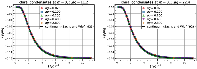
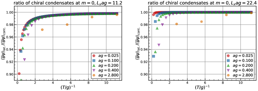
Figure 1: (Upper half) The two analytical chiral condensates (18, 20) as a function of temperature at $L_{x}ag=11.2$ (left) and $L_{x}ag=22.4$ (right). (Lower half) Ratio of the two analytical chiral condensates at the same parameters.

3.2 Chiral condensate at $m\neq 0$

We next calculate the chiral condensate at $m\neq 0,\theta=0$. While there exists no analytically exact result, the chiral condensates at both zero and nonzero temperatures have been extensively studied using the tensor network method Buyens:2014pga ; Banuls:2016lkq ; Buyens:2016ecr . We compare our results with theirs and check the lattice formulation. We stress that this serves as another nontrivial check since we are dealing with the normal ordering dynamically in this case. In this subsection, we remove the logarithmic divergence in the chiral condensate at $m\neq 0$ by subtracting the free chiral condensate at (almost) zero temperature following Refs. Buyens:2014pga ; Banuls:2016lkq ; Buyens:2016ecr . We use the jackknife method to estimate statistical errors.

The chiral condensates at $T/g=\quantity(448\times 0.025)^{-1}$ obtained in this work and the most recent results by the tensor network method at zero temperature Banuls:2016lkq are summarized in Table 2. Our numerical results match theirs with approximately one percent accuracy. It is notable that our results are obtained with no continuum nor infinite spatial length extrapolation in contrast to the tensor network calculations, although the errors are far larger. If one aims at the precision of Ref. Banuls:2016lkq using the current lattice parameters, around $N_{\mathrm{conf}}=10^{10}\text{--}10^{12}$ configurations are required, which is not practically feasible.

$m/g$	This work	Ref. Banuls:2016lkq	This work / Ref. Banuls:2016lkq
0.0625	0.11506(91)	0.1139657(8)	1.0096(80)
0.125	0.09249(66)	0.0920205(5)	1.0051(72)
0.25	0.06629(62)	0.0666457(3)	0.9947(93)
0.5	0.04207(37)	0.0423492(20)	0.9935(87)
1	0.02385(22)	0.0238535(28)	0.9997(93)

Table 2: Absolute values of the chiral condensates at $T/g=\quantity(448\times 0.025)^{-1}$ obtained in this work, compared with the tensor network results at zero temperature Banuls:2016lkq .

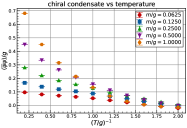
Figure 2: Temperature dependence of the chiral condensate at $m/g=0.0625,0.125,0.25,0.5,1$.

The present method is advantageous at finite temperatures. Figure 2 shows the temperature dependence of the chiral condensate at $m/g=0.0625,0.125,0.25,0.5,1$. Our numerical results are seemingly consistent with the tensor network results Banuls:2016lkq ; Buyens:2016ecr (see Fig. 4 in Ref. Buyens:2016ecr ), and we achieve better precision at high temperatures. Those results provide further evidence that the lattice formulation of the bosonized Schwinger model is valid.

3.3 Finite $\theta$

After verifying the formulation, we next study the Schwinger model with a $\theta$ term, which is inaccessible by the standard Monte Carlo simulation based on the conventional lattice formulation due to the sign problem. In the present method, no difficulty exists. Figure 3 shows the $\theta$ dependences of the chiral condensates

$$\expectationvalue{\overline{\psi}\psi}_{\theta}=-\frac{e^{\gamma}}{2\pi^{3/2}}g\mathcal{O}(1/ag)\expectationvalue{\cos(2\sqrt{\pi}\phi)}_{\theta}$$ (22)

at $m/g=0.0625,0.125,0.25,0.5$. Here Monte Carlo configurations only at $\theta\leq\pi$ are generated, and data points at $\theta>\pi$ are obtained using the line symmetry at $\theta=\pi$. The statistical errors are all smaller than the symbols, even though the chiral condensates at nonzero $\theta$ are evaluated using $N_{\mathrm{conf}}=10^{5}$ configurations. The chiral condensates at $m/g=0.0625,0.125,0.25$ are compared with the leading-order mass perturbation Adam:1997wt ; Adam:1998tw

$$\expectationvalue{\overline{\psi}\psi}_{\theta}-\expectationvalue{\overline{\psi}\psi}_{\theta=0}=\frac{e^{\gamma}}{2\pi^{3/2}}g\quantity(1-\cos\theta)-0.358m\quantity(1-\cos 2\theta).$$ (23)

The mass perturbation theory works well at $m/g=0.0625,0.125$, whereas sizable deviations appear at $m/g=0.25$. These behaviors are consistent with the tensor network results at zero temperature Buyens:2017crb ; Funcke:2019zna , although we are calculating the chiral condensates at very low yet not zero temperature $T/g=(448\times 0.025)^{-1}$.

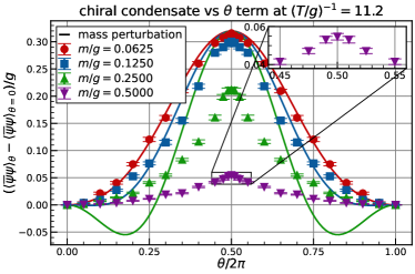
Figure 3: $\theta$ dependence of the chiral condensate at $m/g=0.0625,0.125,0.25,0.5,T/g=\quantity(448\times 0.025)^{-1}$. The chiral condensates at $m/g=0.0625,0.125,0.25$ are compared with the leading-order mass perturbation (23) (solid line).

A cusp-like behavior is observed at $\theta=\pi,m/g=0.5$ in Fig. 3, which might suggest the spontaneous CP symmetry breaking. It is well known that the spontaneous CP symmetry breaking occurs at zero temperature for sufficiently large fermion masses $m/g\gtrsim 0.33$ Coleman:1976uz ; Hamer:1982mx ; Ranft:1982bi ; Byrnes:2002nv ; Shimizu:2014fsa ; Buyens:2017crb ; Azcoiti:2017mxl ; Thompson:2021eze . The analogy with the quantum Ising chain and a tensor network study Buyens:2016ecr suggest that the CP symmetry is restored at any nonzero temperature. To give a definitive answer to this issue, a very careful finite-size scaling analysis is required. Although such a study would be meaningful, we leave it as a future study and turn our attention to confining properties in the Schwinger model at finite temperature and $\theta$.

4 Confinement at finite temperature and $\theta$

We finally investigate confinement/deconfinement properties in the Schwinger model at finite temperature and $\theta$. For this purpose, we calculate the string tension in the $(T,\theta)$ plane.

Let us explain our method to calculate the string tension. Because the $\theta$ angle is physically interpreted as the background electric field $E_{\mathrm{ex}}=(\theta/2\pi)g$ Coleman:1976uz , the inclusion of the two static probe charges $q_{p}g,-q_{p}g$ separated infinity can be described through a modification of the $\theta$ angle:

$$\theta\to 2\pi q_{p}+\theta.$$ (24)

The string tension (coefficient of the linear term in the static potential) between two static probe charges $q_{p}g,-q_{p}g$ can be obtained from the difference in free energy densities

$$\sigma(q_{p},\theta)=f(2\pi q_{p}+\theta)-f(\theta)=\frac{-1}{L_{x}L_{\tau}a^{2}}\ln\frac{Z(2\pi q_{p}+\theta)}{Z(\theta)},$$ (25)

where $Z(\theta)$ is the partition function

$$Z(\theta)=\tr e^{-H(\theta)/T}\propto\int D\phi\,e^{-S_{E}(\theta)}.$$ (26)

The computation of the free energy density itself is difficult by the Monte Carlo method since it cannot be expressed as an expectation value. However, the difference can be:

$$\sigma(q_{p},\theta)=\frac{-1}{L_{x}L_{\tau}a^{2}}\ln\expectationvalue{\exp[-\frac{\quantity(ag)^{2}}{\sqrt{\pi}}\sum_{x,\tau}q_{p}\quantity(\phi_{x,\tau}+\frac{\theta+\pi q_{p}}{2\sqrt{\pi}})]}_{\theta}.$$ (27)

In practical numerical simulations, direct evaluation using Eq. (27) leads to large statistical and systematic errors at large $q_{p}$. To avoid this problem, we consider to decompose the string tension at

$$q_{p}=N\delta q_{p},\quad\theta=M\delta\theta,\quad N,M\in\mathbb{Z},$$ (28)

where $\delta q_{p},\delta\theta$ are some small step widths. When $\delta q_{p}=\delta\theta/2\pi$, the free energy density can be expressed as

$$f(2\pi q_{p}+\theta)=f((N+M)\delta\theta)\eqqcolon f_{N+M}.$$ (29)

Using this notation, the string tension can be decomposed as follows

$$\sigma(N\delta q_{p},M\delta\theta) =f_{N+M}-f_{M}$$ (30a)

$$=\sum_{i=0}^{N-1}f_{i+M+1}-f_{i+M}$$ (30b)

$$=\frac{-1}{L_{x}L_{\tau}a^{2}}\sum_{i=0}^{N-1}\ln\expectationvalue{\exp[-\frac{\quantity(ag)^{2}}{\sqrt{\pi}}\sum_{x,\tau}\delta q_{p}\quantity(\phi_{x,\tau}+\frac{\theta+\pi\delta q_{p}}{2\sqrt{\pi}})]}_{\theta=\quantity(i+M)\delta\theta}.$$ (30c)

By using Eq. (30c) instead of Eq. (27), we can greatly mitigate the large statistical and systematic errors at large $q_{p}$ since $q_{p}$ in Eq. (27) is now replaced by $\delta q_{p}$.

Figure 4 shows the probe charge dependence of the string tension at $ag=0.4,0.2,0.1$ and $m/g=0.25,0.5$. The results are obtained from $N_{\mathrm{conf}}=10^{6}$ configurations at $\theta/\pi$ ranging from $0.0$ to $1.0$ with a step width of $\delta\theta/\pi=0.1$. The temperature and spatial length are held constant at $T/g=11.2^{-1}$ and $L_{x}ag=22.4$, respectively. We find that the results at $ag=0.4,0.2,0.1$ exhibit exceptional precision and agreement. Motivated by this, we use the lattice of $ag=0.2,L_{x}=112$ in the following analysis.

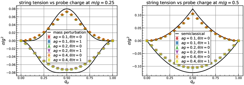
Figure 4: Probe charge dependence of the string tension for $\theta=0,\pi$ at $m/g=0.25$ (left) and $m/g=0.5$ (right). The string tensions at $m/g=0.25$ and $m/g=0.5$ are compared with the mass perturbation (32) and the semiclassical estimates (31), respectively. The temperature and spatial length are held constant at $T/g=11.2^{-1}$ and $L_{x}ag=22.4$, respectively.

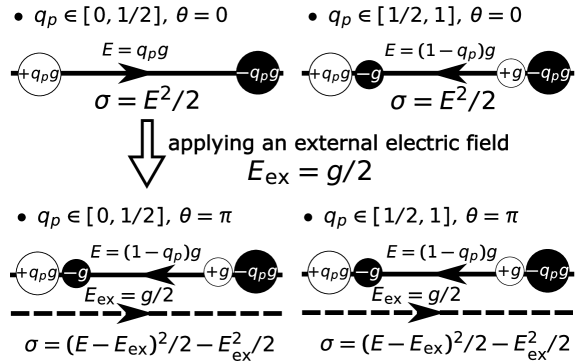
Figure 5: Semiclassical picture of the string tension between two static probe charges $q_{p}g,-q_{p}g$.

In Fig. 4, we observe peculiar behaviors in the string tension: at $\theta=0$, there is a peak in the string tension at $q_{p}=0.5$. More interestingly, the string tension becomes negative for noninteger probe charges at $\theta=\pi$. These behaviors can be well understood through semiclassical analysis of the string tension (see Fig. 5). For $q_{p}\in\quantity[0,1/2],\theta=0$, a constant electric field $E=q_{p}g$ appears between the two static probe charges at the classical level due to the Gauss law, as shown in the upper left of Fig. 5. Consequently, the string tension increases quadratically as the probe charge $q_{p}$ increases. When $q_{p}$ exceeds $1/2$, and the distance between the probe charges is sufficiently large, the vacuum produces a fermion-antifermion pair, reducing the total electric field by forming a two “meson” system (upper right of Fig. 5). Setting $\theta=\pi$, i.e., applying an external electric field $E_{\mathrm{ex}}=g/2$, to the two “meson” system, the external electric field works to decrease the total electric field, resulting in the negative string tension. In the case of the single “meson” system (upper left of Fig. 5), as the external electric field approaches $g/2$, the vacuum would again produce a fermion-antifermion pair to decrease the total electric field by forming a two “meson“ system at a certain value of $\theta$. Therefore, at $\theta=\pi$, the configuration is the same regardless of the probe charge, as shown in the lower of Fig. 5. The resulting semiclassical estimate for the string tension is then given by

$$\sigma/g^{2}=\begin{cases}\frac{1}{2}q_{p}^{2},&q_{p}\in\quantity[0,\frac{1}{2}],\,\theta=0,\\ \frac{1}{2}\quantity(1-q_{p})^{2},&q_{p}\in\quantity[\frac{1}{2},1],\,\theta=0,\\ -\frac{1}{2}q_{p}\quantity(1-q_{p}),&q_{p}\in\quantity[0,1],\,\theta=\pi.\end{cases}$$ (31)

In the right panel of Fig. 4, we find that the semiclassical string tension (31) successfully explains the qualitative behaviors of our numerical results.

While it is hard to give an intuitive explanation for the negative string tension at small fermion mass, the next-to-leading order mass perturbation Adam:1996rd ; Adam:1997wt

$$\sigma/g^{2}=\frac{e^{\gamma}}{2\pi^{3/2}}\frac{m}{g}\quantity(\cos(\theta)-\cos(2\pi q_{p}+\theta))-0.179\quantity(\frac{m}{g})^{2}\quantity(\cos(2\theta)-\cos(4\pi q_{p}+2\theta))$$ (32)

successfully explains the qualitative behaviors, as shown in the left panel of Fig. 4. We note that the string tensions at $\theta=0$ at various masses, probe charges, and temperatures have been already obtained with high precision by the tensor network method Buyens:2015tea ; Buyens:2016ecr ; Buyens:2017crb . However, the string tension at nonzero $\theta$ has not been investigated well so far. In the case of the charge-$3$ Schwinger model, the string tension between integer probe charges at nonzero $\theta$ was studied in Ref. Honda:2021ovk through quantum simulation on a classical simulator. Negative string tension was observed at large $\theta$, although reliable continuum extrapolation was difficult due to a limited number of lattice sites ($N\leq 25$) and slow convergence to the continuum limit. In Refs. Misumi:2019dwq ; Honda:2021ovk , the negative string tension between integer probe charges in the charge-$q$ Schwinger model, where $q$ is an integer larger than $1$, was explained in terms of the $\mathbb{Z}_{q}$ 1-form symmetry. Unfortunately, their argument can not be applied to the present case. Nevertheless, our numerical results demonstrate that the negative string tension appears for noninteger probe charges at almost zero temperature in the standard Schwinger model.

After confirming the effectiveness of our method in calculating the string tension and giving an intuitive physical explanation, we explain our simulation strategy to establish the string tension in the $(T,\theta)$ plane. To cover almost the entire $(T,\theta)$ plane, we generate $N_{\mathrm{conf}}=10^{6}$ Monte Carlo configurations at $L_{\tau}=4,6,8,10,12,16,20,24,28,40,56$, with $\theta/\pi$ ranging from $0.0$ to $1.0$ with a step width of $\delta\theta/\pi=0.1$. By combining these configurations with the reweighing method, we achieve a very smooth surface in the $(T,\theta)$ plane. For both $T$ and $\theta$ directions, we obtain ten data points between adjacent simulation points, each reweighted from the nearest simulation point. This results in $12^{2}$ data points within the unit cell formed by four simulation points.

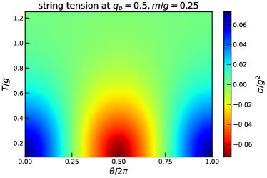
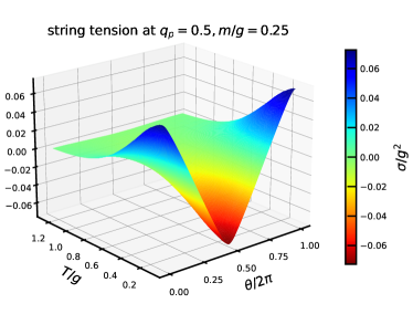
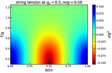
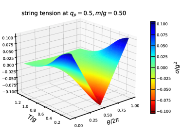
Figure 6: The string tension at $q_{p}=0.5$ in the $(T,\theta)$ plane at $m/g=0.25$ (upper half) and $m/g=0.5$ (lower half).

Figure 6 shows the string tension at $q_{p}=0.5$ in the $(T,\theta)$ plane at $m/g=0.25$ (upper half) and $m/g=0.5$ (lower half). At $q_{p}=0.5$, one can easily show that

$$\sigma(0.5,\theta+\pi)=-\sigma(0.5,\theta).$$ (33)

For both $m/g=0.25$ and $m/g=0.5$, the string tension is positive around $\theta\simeq 0$ at low temperatures, indicating confinement. The string tension diminishes as $\theta$ increases and becomes zero at $\theta/\pi=0.5$. With further increases in $\theta$, the string tension becomes negative and reaches its minimum at $\theta=\pi$. The peak height is roughly proportional to the fermion mass $m/g$. As temperature increases, the string tension gradually converges to zero at all $\theta$, indicating deconfinement. In Fig. 7, we show similar plots but at $q_{p}=0.3$, where simple constraint like Eq. (33) does not exist. Consequently, we observe shifts of the peak positions. Nevertheless, the basic pattern remains the same: the system undergoes a smooth transition from the confining phase to the inverse confining phase as $\theta$ goes from $0$ to $\pi$, and this transition becomes weakened as temperature increases.

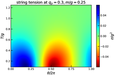
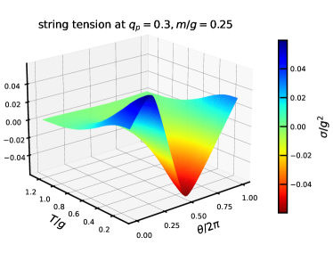
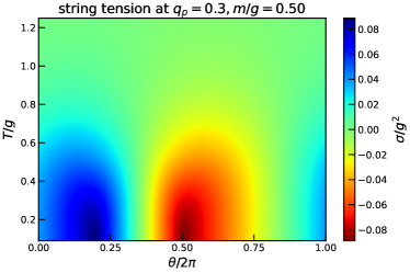
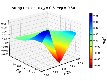
Figure 7: The string tension at $q_{p}=0.3$ in the $(T,\theta)$ plane at $m/g=0.25$ (upper half) and $m/g=0.5$ (lower half).

5 Summary and future study

In this paper, we have revisited the lattice formulation of the bosonized Schwinger model of Bender et al. in 1985 Bender:1984qg and shed new light on it as a method for circumventing the sign problem. After conducting a comprehensive review of their accomplishment, we have verified the formulation by reproducing the analytical chiral condensate at $m=0$ and also by comparing our numerical results at $m\neq 0$ with previous numerical studies. As an application, we have studied confining properties in the Schwinger model at finite temperature and $\theta$. We have established the string tension in the $(T,\theta)$ plane for the first time and revealed the confining properties in the Schwigner model quantitatively. In particular, we found that the string tension is negative for noninteger probe charges around $\theta=\pi$ at low temperatures.

The present method has both advantages and drawbacks compared to spin Hamiltonian approaches. Because of the fast convergence to the continuum limit and low numerical cost, no continuum nor infinite spatial length extrapolation is needed in practice, as was demonstrated in this paper. Also, thermal expectation values can be very easily calculated in the method. On the other hand, expectation values at exactly zero temperature cannot be obtained. Moreover, it seems very hard to achieve the precision of the tensor network method at zero temperature. Thus, these two approaches complement each other and would promote further understanding of the Schwinger model. In particular, investigating the fate of CP symmetry at finite temperature would be an attractive future study, which can be pursued using the present method.

As another future study, the application of the lattice formulation to other models would be intriguing. The work of Bender et al. has revealed that it is possible to formulate a bosonized fermionic model on a lattice even with a nontrivial interaction, at least in the case of the Schwinger model. An important question that arises here is the feasibility of applying the lattice formulation to other fermionic models in one spatial dimension, such as the multi-flavor Schwinger model, the gauged Thirring model, one-dimensional QCD, and so on. Because the key formula (9) is model-independent, and bosonization is a rather universal concept in one spatial dimension, the lattice formulation is expected to be applicable to a wide variety of fermionic models.

- (1) J.S. Schwinger, Gauge Invariance and Mass. 2., Phys. Rev. 128 (1962) 2425.
- (2) S.R. Coleman, The Quantum Sine-Gordon Equation as the Massive Thirring Model, Phys. Rev. D 11 (1975) 2088.
- (3) S. Mandelstam, Soliton Operators for the Quantized Sine-Gordon Equation, Phys. Rev. D 11 (1975) 3026.
- (4) S.R. Coleman, R. Jackiw and L. Susskind, Charge Shielding and Quark Confinement in the Massive Schwinger Model, Annals Phys. 93 (1975) 267.
- (5) S.R. Coleman, More About the Massive Schwinger Model, Annals Phys. 101 (1976) 239.
- (6) W. Fischler, J.B. Kogut and L. Susskind, Quark Confinement in Unusual Environments, Phys. Rev. D 19 (1979) 1188.
- (7) N.S. Manton, The Schwinger Model and Its Axial Anomaly, Annals Phys. 159 (1985) 220.
- (8) S. Iso and H. Murayama, Hamiltonian Formulation of the Schwinger Model: Nonconfinement and Screening of the Charge, Prog. Theor. Phys. 84 (1990) 142.
- (9) J.E. Hetrick and Y. Hosotani, QED ON A CIRCLE, Phys. Rev. D 38 (1988) 2621.
- (10) A.V. Smilga, On the fermion condensate in Schwinger model, Phys. Lett. B 278 (1992) 371.
- (11) A.V. Smilga, Critical amplitudes in two-dimensional theories, Phys. Rev. D 55 (1997) 443 [hep-th/9607154].
- (12) I. Sachs and A. Wipf, Finite temperature Schwinger model, Helv. Phys. Acta 65 (1992) 652 [1005.1822].
- (13) T.M.R. Byrnes, P. Sriganesh, R.J. Bursill and C.J. Hamer, Density matrix renormalization group approach to the massive Schwinger model, Phys. Rev. D 66 (2002) 013002 [hep-lat/0202014].
- (14) M.C. Bañuls, K. Cichy, K. Jansen and J.I. Cirac, The mass spectrum of the Schwinger model with Matrix Product States, JHEP 11 (2013) 158 [1305.3765].
- (15) B. Buyens, J. Haegeman, K. Van Acoleyen, H. Verschelde and F. Verstraete, Matrix product states for gauge field theories, Phys. Rev. Lett. 113 (2014) 091601 [1312.6654].
- (16) Y. Shimizu and Y. Kuramashi, Grassmann tensor renormalization group approach to one-flavor lattice Schwinger model, Phys. Rev. D 90 (2014) 014508 [1403.0642].
- (17) Y. Shimizu and Y. Kuramashi, Critical behavior of the lattice Schwinger model with a topological term at using the Grassmann tensor renormalization group, Phys. Rev. D 90 (2014) 074503 [1408.0897].
- (18) B. Buyens, K. Van Acoleyen, J. Haegeman and F. Verstraete, Matrix product states for Hamiltonian lattice gauge theories, PoS LATTICE2014 (2014) 308 [1411.0020].
- (19) M.C. Bañuls, K. Cichy, J.I. Cirac, K. Jansen and H. Saito, Thermal evolution of the Schwinger model with Matrix Product Operators, Phys. Rev. D 92 (2015) 034519 [1505.00279].
- (20) B. Buyens, J. Haegeman, H. Verschelde, F. Verstraete and K. Van Acoleyen, Confinement and string breaking for QED2 in the Hamiltonian picture, Phys. Rev. X 6 (2016) 041040 [1509.00246].
- (21) M.C. Bañuls, K. Cichy, K. Jansen and H. Saito, Chiral condensate in the Schwinger model with Matrix Product Operators, Phys. Rev. D 93 (2016) 094512 [1603.05002].
- (22) B. Buyens, F. Verstraete and K. Van Acoleyen, Hamiltonian simulation of the Schwinger model at finite temperature, Phys. Rev. D 94 (2016) 085018 [1606.03385].
- (23) M.C. Bañuls, K. Cichy, J.I. Cirac, K. Jansen and S. Kühn, Density Induced Phase Transitions in the Schwinger Model: A Study with Matrix Product States, Phys. Rev. Lett. 118 (2017) 071601 [1611.00705].
- (24) B. Buyens, S. Montangero, J. Haegeman, F. Verstraete and K. Van Acoleyen, Finite-representation approximation of lattice gauge theories at the continuum limit with tensor networks, Phys. Rev. D 95 (2017) 094509 [1702.08838].
- (25) L. Funcke, K. Jansen and S. Kühn, Topological vacuum structure of the Schwinger model with matrix product states, Phys. Rev. D 101 (2020) 054507 [1908.00551].
- (26) E. Ercolessi, P. Facchi, G. Magnifico, S. Pascazio and F.V. Pepe, Phase Transitions in Gauge Models: Towards Quantum Simulations of the Schwinger-Weyl QED, Phys. Rev. D 98 (2018) 074503 [1705.11047].
- (27) S. Kühn, J.I. Cirac and M.-C. Bañuls, Quantum simulation of the Schwinger model: A study of feasibility, Phys. Rev. A 90 (2014) 042305 [1407.4995].
- (28) T.V. Zache, N. Mueller, J.T. Schneider, F. Jendrzejewski, J. Berges and P. Hauke, Dynamical Topological Transitions in the Massive Schwinger Model with a Term, Phys. Rev. Lett. 122 (2019) 050403 [1808.07885].
- (29) C. Kokail et al., Self-verifying variational quantum simulation of lattice models, Nature 569 (2019) 355 [1810.03421].
- (30) G. Magnifico, M. Dalmonte, P. Facchi, S. Pascazio, F.V. Pepe and E. Ercolessi, Real Time Dynamics and Confinement in the Schwinger-Weyl lattice model for 1+1 QED, Quantum 4 (2020) 281 [1909.04821].
- (31) B. Chakraborty, M. Honda, T. Izubuchi, Y. Kikuchi and A. Tomiya, Classically emulated digital quantum simulation of the Schwinger model with a topological term via adiabatic state preparation, Phys. Rev. D 105 (2022) 094503 [2001.00485].
- (32) M. Honda, E. Itou, Y. Kikuchi, L. Nagano and T. Okuda, Classically emulated digital quantum simulation for screening and confinement in the Schwinger model with a topological term, Phys. Rev. D 105 (2022) 014504 [2105.03276].
- (33) S. Thompson and G. Siopsis, Quantum computation of phase transition in the massive Schwinger model, Quantum Sci. Technol. 7 (2022) 035001 [2110.13046].
- (34) M. Honda, E. Itou, Y. Kikuchi and Y. Tanizaki, Negative string tension of a higher-charge Schwinger model via digital quantum simulation, PTEP 2022 (2022) 033B01 [2110.14105].
- (35) J.C. Halimeh, I.P. McCulloch, B. Yang and P. Hauke, Tuning the Topological -Angle in Cold-Atom Quantum Simulators of Gauge Theories, PRX Quantum 3 (2022) 040316 [2204.06570].
- (36) QuNu collaboration, Variational thermal quantum simulation of the lattice Schwinger model, Phys. Rev. D 106 (2022) 054509 [2205.12767].
- (37) C. Gattringer, T. Kloiber and V. Sazonov, Solving the sign problems of the massless lattice Schwinger model with a dual formulation, Nucl. Phys. B 897 (2015) 732 [1502.05479].
- (38) D. Göschl, C. Gattringer, A. Lehmann and C. Weis, Simulation strategies for the massless lattice Schwinger model in the dual formulation, Nucl. Phys. B 924 (2017) 63 [1708.00649].
- (39) Y. Tanizaki and M. Tachibana, Multi-flavor massless QED2 at finite densities via Lefschetz thimbles, JHEP 02 (2017) 081 [1612.06529].
- (40) A. Alexandru, G. Başar, P.F. Bedaque, H. Lamm and S. Lawrence, Finite Density Near Lefschetz Thimbles, Phys. Rev. D 98 (2018) 034506 [1807.02027].
- (41) I. Bender, H.J. Rothe and K.D. Rothe, Monte Carlo Study of Screening Versus Confinement in the Massless and Massive Schwinger Model, Nucl. Phys. B 251 (1985) 745.
- (42) J.B. Kogut and L. Susskind, Hamiltonian Formulation of Wilson’s Lattice Gauge Theories, Phys. Rev. D 11 (1975) 395.
- (43) T. Matsubara, A New approach to quantum statistical mechanics, Prog. Theor. Phys. 14 (1955) 351.
- (44) M. Creutz, Monte Carlo Study of Quantized SU(2) Gauge Theory, Phys. Rev. D 21 (1980) 2308.
- (45) C. Adam, Massive Schwinger model within mass perturbation theory, Annals Phys. 259 (1997) 1 [hep-th/9704064].
- (46) C. Adam, Normalization of the chiral condensate in the massive Schwinger model, Phys. Lett. B 440 (1998) 117 [hep-th/9806211].
- (47) C.J. Hamer, J.B. Kogut, D.P. Crewther and M.M. Mazzolini, The Massive Schwinger Model on a Lattice: Background Field, Chiral Symmetry and the String Tension, Nucl. Phys. B 208 (1982) 413.
- (48) J. Ranft and A. Schiller, Local Hamiltonian Monte Carlo Study of the Massive Schwinger Model in an External Background Field, Phys. Lett. B 122 (1983) 403.
- (49) V. Azcoiti, E. Follana, E. Royo-Amondarain, G. Di Carlo and A. Vaquero Avilés-Casco, Massive Schwinger model at finite , Phys. Rev. D 97 (2018) 014507 [1709.07667].
- (50) C. Adam, Charge screening and confinement in the massive Schwinger model, Phys. Lett. B 394 (1997) 161 [hep-th/9609155].
- (51) T. Misumi, Y. Tanizaki and M. Ünsal, Fractional angle, ’t Hooft anomaly, and quantum instantons in charge- multi-flavor Schwinger model, JHEP 07 (2019) 018 [1905.05781].