Integrating Automatic and Manual Reserves in Optimal Power Flow via Chance Constraints

Abstract

Uncertainty in renewable energy generation has the potential to adversely impact the operation of electric power systems. Numerous approaches to manage this impact have been proposed, ranging from stochastic and chance-constrained programming to robust optimization. However, these approaches either tend to be conservative in their assumptions, causing higher-than-necessary costs, or leave the system vulnerable to low probability, high impact uncertainty realizations. To address this issue, we propose a new formulation for stochastic optimal power flow that explicitly distinguishes between “normal operation”, in which automatic generation control (AGC) is sufficient to guarantee system security, and “adverse operation”, in which the system operator is required to take additional actions, e.g., manual reserve deployment. This formulation can be understood as a combination of a joint chance-constrained problem, which enforces that AGC should be sufficient with a high probability, with specific treatment of large-disturbance scenarios that allows for additional, more complex redispatch actions. The new formulation has been compared with the classical ones in a case study on the IEEE-118 bus system. We observe that our consideration of extreme scenarios enables solutions that are more secure than typical chance-constrained formulations, yet less costly than solutions that guarantee robust feasibility with only AGC.

Nomenclature

The main notation used throughout the text is stated below for quick reference.

-A Sets

• Set of generating units, indexed by $g$.

• Set of transmission lines, indexed by $l$.

• Set of nodes, indexed by $n$.

-B Parameters

• Linear operating cost of generating unit $g$ [€/MWh].

• Downward/Upward reserve capacity cost of generating unit $g$ [€/MW].

• Downward/Upward reserve cost of generating unit $g$ [€/MWh].

• Power transfer distribution factor (PTDF) of transmission line $l$ with respect to node $n$.

• Forecasted demand at node $n$ [MW].

• Maximum capacity of transmission line $l$ [MW].

• Minimum/Maximum output of unit $g$ [MW].

• Ability of generator $g$ to provide downward and upward reserves [MW].

• Actual wind power production at node $n$ [MW].

• Forecasted wind power production at node $n$ [MW].

• Error of the predicted wind power at node $n$ [MW].

-C Variables

• Power output dispatch of unit $g$ [MW].

• Reserve deployed by unit $g$ [MW].

• Downward/Upward reserve deployed by unit $g$ [MW].

• Downward/Upward reserve capacity of unit $g$ [MW].

• Manual adjustment of power output dispatch at unit $g$ [MW].

• Participation factor of unit $g$.

I Introduction

The Optimal Power Flow (OPF) is a classical tool widely used for day-ahead and real-time power system operations, electricity markets, long-term planning, and many other applications [1, 2, 3]. In its deterministic version, the OPF problem seeks to determine the least-costly dispatch of thermal generating units to satisfy the system’s demand, while complying with the technical limits of production and transmission network equipment [4]. However, the increasing integration of renewable energy sources into power systems leads to increased variability and uncertainty in both the power generation and associated power flows. Understanding and quantifying the impact of this uncertainty on decision-making problems such as the OPF is crucial to ensure the secure operation of power systems [5].

Given this context, a large and growing body of work has addressed the stochastic version of the optimal power flow (SOPF) problem [6]. The SOPF aims to minimize expected operational cost and avoid constraint violations while considering the uncertainty in its random parameters. Existing works deal with uncertainty in SOPF using different approaches such as multi-stage stochastic programming [7], robust or worst-case optimization [8, 9, 10] or chance-constraints [11, 12, 13, 14, 15, 16, 17, 18]. The major challenge is to design a model that captures the risk of constraint violations and accurately reflects the operation of power systems, while maintaining computational tractability.

When modeling the impact of uncertain generation on short-term operations (i.e. day-ahead until real-time), it is common to assume that forecast errors and renewable energy variability will be balanced by the deployment of generation reserves, and in particular, by systems such as the automatic generation control (AGC) [19]. A benefit of modeling system balancing through AGC is that it is naturally represented as an affine control policy, which also simplifies the solution of the optimization problem. However, the common AGC models implemented in the literature typically assume that all generators contribute reserve power according to the affine policy, even for large uncertainty deviations. In reality, generator output will saturate (or stop increasing/decreasing as the deviation grows larger) when they hit their lower or upper generation limit. Furthermore, operators generally take additional actions to manage both balancing and congestion in situations with very large deviations. For example, the North American Reliability Corporation (NERC) [20] standard for regulating the use of AGC, BAL-005, states that if the AGC becomes inoperative or may impair the reliability of the interconnection, the system operator must use manual controls to adjust generation in order to guarantee balance.

While a limited number of studies have shown that modeling generation saturation [21] or accounting for manual reserve activation during large deviations [22] leads to better operating conditions, these models are often computationally expensive. Thus, a more common approach is to apply the affine control policy, but explicitly disregard constraint satisfaction in a fraction of the most severe operating conditions. This is typically done by introducing chance constraints that allow violations in a (typically small) percentage of scenarios [23, 11, 12, 14, 15, 16, 17, 18], or by solving robust optimization formulations where the uncertainty set has been designed to contain a certain probability mass [24]. Unfortunately, by failing to model the impact of the worst scenarios (those for which the constraint satisfaction is discarded), a chance-constrained formulation may leave the system vulnerable to large disruptions that include generator and line outages, or load shed. As discussed in [14], there could be instances where the combination of generators and renewable outputs collude to produce power flows that significantly exceed the nominal line ratings, even in the absence of a large total power deviation. When the maximum rating of a line is exceeded, this line becomes more likely to trip, leaving the network vulnerable to cascading failures and associated load shed.

To address this issue, in this work we propose a new SOPF formulation where, in the worst-case scenarios, operators account for additional reserve to reduce their impact. The proposed formulation distinguishes between two different operating regimes: normal operation and adverse operation. In normal operation, AGC is sufficient to maintain the system balance, while in adverse operation, the system operator may need to implement additional actions, such as manual adjustments, to preserve system security.

Unlike the standard joint chance-constrained OPF (JCC-OPF), which limits the joint probability of violation of technical constraints, our formulation uses a joint chance-constraint to control the probability of utilizing different reserve actions. Thus, we can impose that AGC alone is to be sufficient with a high probability, while additional corrective actions are only to be implemented for the most adverse scenarios. In doing so, we reduce the need for frequent manual intervention by operators (computational expensive), while also guaranteeing that additional resources are available to handle adverse operating conditions, e.g., by scheduling more reserve capacity for manual deployment.

To demonstrate the suitability of our proposed formulation, we conduct a computational experiment that compared it to two state-of-the-art approaches. The former is the standard JCC-OPF, whose drawback is to leave the power system vulnerable to severe events, e.g., by dispatching insufficient generation capacity or giving up on alleviating congestion. The second approach guarantees robust feasibility using AGC only, which results in conservative solutions with increased operating costs, for instance, due to inefficient and oversized generation capacity. Our novel formulation results in decisions that are more reliable than the former approach and more cost-efficient than the latter.

The main contributions of our work are thus the following:

• We propose a novel formulation that accounts for various reserve actions employed in actual power system operations, such as AGC and manual re-dispatch.

• We use a joint chance constraint to restrict the probability of manual adjustments occurring instead of limiting the probability of violation of technical constraints. Hence, we consider a more realistic setting where the AGC operates under ordinary system conditions and the manual adjustments, which are not automatic, are implemented under adverse scenarios only.

• We show that our approach yields solutions that are more reliable than the conventional joint chance-constrained DC-OPF, yet less costly than those approaches that guarantee robust feasibility.

The rest of this paper is organized as follows. Section II describes the proposed SOPF formulation, which is derived from two traditional approaches in the literature. Section III describes the reformulation and algorithm used to make our proposal tractable and computationally efficient. Section IV explains the methodology we use to benchmark our approach, while Section V discusses experimental results from a case study. Finally, conclusions are duly drawn in Section VI.

II Problem Formulation

We start this section by introducing a standard and well-known formulation of the joint chance-constrained DC-OPF problem, which will serve us a basis to construct and motivate our proposal immediately after. To lighten the formulation of this problem, we assume that there is one dispatchable generator, one uncertain power source (e.g., a wind farm) and one power load per node $n$. The power dispatch of the generator, the power produced by the uncertain power source and the power consumed by the power load are denoted by $p_{n}$, $\tilde{w}_{n}$, and $d_{n}$, respectively.

The power $\tilde{w}_{n}$ generated by the uncertain power source at node $n$ is modeled as a random variable, which we decompose as $\tilde{w}_{n}=\widehat{w}_{n}+\omega_{n}$, with $\widehat{w}_{n}$ being the forecast value (assumed unbiased) and $\omega_{n}$ the associated forecast error. The system-wide aggregate forecast error is given by $\Omega=\sum_{n\in\mathcal{N}}\omega_{n}$, which is balanced by the dispatchable generators through the deployment of reserve. The reserve deployment follows an affine control policy, modeling the actions of the Automatic Generation Control (AGC). According to this policy, the reserve provided by the generator at node $n$ is given by $r_{n}(\boldsymbol{\omega})=-\beta_{n}\Omega$, where $\beta_{n}$ is the participation factor and $\boldsymbol{\omega}$ represents the vector of power forecast errors across all nodes. Furthermore, we distinguish between upward or positive reserve $r^{+}_{n}(\boldsymbol{\omega})$ and downward or negative reserve $r^{-}_{n}(\boldsymbol{\omega})$, with $r_{n}(\boldsymbol{\omega})=r^{+}_{n}(\boldsymbol{\omega})-r^{-}_{n}(\boldsymbol{\omega})$.

With this notation in place, the joint chance-constrained DC-OPF problem can be formulated as follows:

$$\min_{\Xi} \quad\sum_{n}c_{n}\,p_{n}+c^{u}_{n}r^{u}_{n}+c^{d}_{n}r^{d}_{n}$$

$$\hskip 56.9055pt+\mathbb{E}\left[c^{+}_{n}r^{+}_{n}(\boldsymbol{\omega})-c^{-}_{n}r^{-}_{n}(\boldsymbol{\omega})\right]$$ (1a)

s.t. $$\sum_{n}\beta_{n}=1$$ (1b)

$$\sum_{n}(p_{n}+\widehat{w}_{n}-d_{n})=0$$ (1c)

$$\underline{p}_{n}+r^{d}_{n}\leq p_{n}\leq\overline{p}_{n}-r^{u}_{n},\quad\forall n$$ (1d)

$$0\leq r^{d}_{n}\leq\overline{r}^{d}_{n},\quad\forall n$$ (1e)

$$0\leq r^{u}_{n}\leq\overline{r}^{u}_{n},\quad\forall n$$ (1f)

$$r^{+}_{n}(\boldsymbol{\omega})-r^{-}_{n}(\boldsymbol{\omega})=-\Omega\beta_{n},\forall n$$ (1g)

$$\mathbb{P}\left(\begin{array}[]{l}-r^{d}_{n}\leq-\Omega\beta_{n}\leq r^{u}_{n},\quad\forall n\\ -\overline{f}_{l}\leq\displaystyle\sum_{n}B_{ln}(p_{n}-\Omega\beta_{n}+\\ \hskip 19.91684pt+\widehat{w}_{n}+\omega_{n}-d_{n})\leq\overline{f}_{l},\forall l\end{array}\right)\geq 1-\epsilon$$ (1k)

$$\beta_{n},r^{+}_{n}(\boldsymbol{\omega}),r^{-}_{n}(\boldsymbol{\omega})\geq 0,\quad\forall n,$$ (1l)

where $\Xi=(p_{n},r^{+}_{n}(\boldsymbol{\omega}),r^{-}_{n}(\boldsymbol{\omega}),r^{d}_{n},r^{u}_{n},\beta_{n})$ is the set of decision variables. We remark that $r^{d}_{n}$ and $r^{u}_{n}$ are the downward and upward reserve capacity provided by the dispatchable generator at node $n$. This reserve capacity is procured by the system operator before the forecast errors $\boldsymbol{\omega}$ are known.

The three terms of the objective function (1a) to be minimized correspond to the power dispatch cost, the cost of procuring reserve capacity, and the expected cost related to the actual deployment of that capacity, respectively. The power balance in the system is guaranteed for all possible realizations of $\boldsymbol{\omega}$ through equations (1b) and (1c). Note that by requiring $\beta_{n}\geq 0$ in (1l), we enforce that all reserve deployment only acts to counterbalance forecast, rather than also allowing redispatch among generators to counter congestion. Constraints (1d) ensure that the power produced by dispatchable generators is within their minimum and maximum power output limits, i.e., $\underline{p}_{n}$ and $\overline{p}_{n}$, respectively, considering the reserve capacity the system operator procures from them. Constraints (1e) and (1f) set a limit on the maximum reserve capacity each generator is willing or able to provide. Equation (1g) models the affine control policy for reserve deployment (AGC) we discussed above. Expression (1k) constitutes the joint chance-constraint system by which the system operator states that the reserves deployed and the line flows must be within their bounds with a probability greater than or equal to $1-\epsilon$. Accordingly, parameter $\epsilon$ is the maximum allowed probability of constraint violation set by the operator. In (1k), $l$ is the index of transmission lines in the power network and $\overline{f}_{l}$ stands for the capacity limit of line $l$. Finally, (1l) imposes the positive character of decision variables $\beta_{n}$ and random functions $r^{+}_{n}(\boldsymbol{\omega})$ and $r^{-}_{n}(\boldsymbol{\omega})$ for all $n$. Note that the probability in (1k) is computed over the probability space of $\boldsymbol{\omega}$ and that the equality (1g) and the inequality (1l) must hold for almost all $\boldsymbol{\omega}$.

The popularity of the joint chance-constrained formulation (1) stems from its ability to reduce the expected system operating cost substantially by allowing the violation of reserve capacity constraints and/or line flow limits under a small $\epsilon$-percentage of realizations of $\boldsymbol{\omega}$. These realizations, or scenarios, are thus the most detrimental to the system in terms of cost. Parameter $\epsilon$ in (1) controls the level of risk aversion of the system operator (the lower, the more risk averse), to the point that if $\epsilon$ is set to $0$, formulation (1) becomes robustly feasible, meaning that all the constraints and variable limits are to be satisfied with probability one.

Nonetheless, the critical nature of power systems practically forces operators to guarantee robust feasibility. In this regard, formulation (1), even if $\epsilon=0$, offers an incomplete picture of how power systems are actually operated. Indeed, in those very few $\boldsymbol{\omega}$-scenarios for which AGC is unable or too costly to ensure the system’s integrity, the operators can still take over the affine control policy and manually set new operating points for some generators in the system, those needed to guarantee the satisfaction of the system’s constraints ideally at the minimum cost. The fact that formulation (1) ignores the possibility of a manual control taking over AGC (albeit with a low occurrence) causes it to underestimate the operating cost when $\epsilon>0$ or overestimate it when robust feasibility is pursued ($\epsilon=0$). The ultimate result is that formulation (1) may produce uneconomical or suboptimal affine control policies.

To illustrate our point, we use an example based on the small power system depicted in Fig. 1. The system includes two thermal generating units with the linear production costs, reserve capacity costs and maximum power limits indicated in the figure. For simplicity, the susceptances of all lines are assumed to be 1 p.u. and the capacity of each line is also specified in the figure. A single demand of 80 MW is located at node $n_{3}$, where there is also a wind farm with a predicted output of 20 MW. We assume that the associated (random) forecast error can take on three different values only, namely, $20$, $10$, and $-20$ MW, corresponding to three equally probable realizations or scenarios 1, 2 and 3, in that order. The costs of deploying upward and downward reserve, i.e., $c^{+}_{n}$ and $c^{-}_{n}$, are 1.2 and 0.8 times the generator’s linear operating cost, respectively.

Results from problem (1) when $\epsilon=1/3$ and $\epsilon=0$ are collated in the first two rows of Table I. These results include the optimal power dispatch, participation factors and procured reserve capacities, together with the optimal expected operating cost. Unsurprisingly, the results are quite sensitive to $\epsilon$. For example, when this is set to zero (to achieve robust feasibility), much more reserve capacity is to be procured than when we allow the system’s constraints to be violated under one of the scenarios, in particular, scenario 3. Accordingly, the cost increases from €95 to €137.5, when $\epsilon$ goes from 1/3 to 0. In contrast, if we take the solution delivered for $\epsilon=1/3$ and scenario 3 actually occurs, meaning that the wind power forecast error takes on the value $-20$MW, the AGC requires generator $g_{2}$ to increase its production up to $65$MW, that is, above its maximum output limit, while exceeding the maximum capacity of line $l_{1}$ too. But what is more important from a practical point of view is that, under such a scenario, the solution to problem (1) when $\epsilon=1/3$ does not allow for any manual re-dispatch that can restore system feasibility immediately after, because no upward reserve capacity has been procured beforehand.

Consequently, formulation (1) may be too risky or too costly. Instead, we propose next a novel joint chance-constrained formulation of the DC-OPF problem that does account for the possibility of resorting to a manual re-dispatch in this $\epsilon$-percentage of events in which the implementation of AGC is too expensive or even infeasible. For this, we replace the set of constraints (1g)–(1k) in (1) with the following ones:

$$\sum_{n}\alpha_{n}(\boldsymbol{\omega})=0$$ (2a)

$$r^{+}_{n}(\boldsymbol{\omega})-r^{-}_{n}(\boldsymbol{\omega})=-\Omega\beta_{n}+\alpha_{n}(\boldsymbol{\omega}),\forall n$$ (2b)

$$-r^{d}_{n}\leq-\Omega\beta_{n}+\alpha_{n}(\boldsymbol{\omega})\leq r^{u}_{n},\quad\forall n$$ (2c)

$$-\overline{f}_{l}\leq\sum_{n}B_{ln}(p_{n}-\Omega\beta_{n}+\alpha_{n}(\boldsymbol{\omega})+$$

$$\hskip 71.13188pt+\widehat{w}_{n}+\omega_{n}-d_{n})\leq\overline{f}_{l},\quad\forall l$$ (2d)

$$\mathbb{P}\left(\alpha_{n}(\boldsymbol{\omega})=0,\quad\forall n\right)\geq 1-\epsilon,$$ (2e)

where $\alpha_{n}(\omega)$ is a random variable that represents the manual adjustment of the power output of the generator located at node $n$.

Equation (2a) is required for the implemented power adjustments to preserve the power balance. Equation (2b) is analogous to (1g), but including the manual adjustment requested by the system operator. Inequalities (2c) and (2d) enforce that the use of AGC in combination with manual re-dispatch guarantees that the system’s constraints are satisfied under any realization of $\boldsymbol{\omega}$. Finally, in our proposal, chance-constrained programming is employed for a different purpose than that in (1). Specifically, the chance-constraint (2e) seeks to characterize the use of manual control as an occassional recourse action, thus ensuring that AGC is the standard control policy. Again constraints (2a)–(2d) are to be satisfied for almost all $\boldsymbol{\omega}$.

Our proposal can thus be formulated as follows:

$$\min_{\Xi}\quad \sum_{n}c_{n}\,p_{n}+c^{u}_{n}r^{u}_{n}+c^{d}_{n}r^{d}_{n}$$

$$\hskip 56.9055pt+\mathbb{E}\left[c^{+}_{n}r^{+}_{n}(\boldsymbol{\omega})-c^{-}_{n}r^{-}_{n}(\boldsymbol{\omega})\right]$$ (3a)

s.t. $$\eqref{eq:JCCOPF_balance1}-\eqref{eq:JCCOPF_maxupres}$$ (3b)

$$\eqref{eq:balance_FJCCOPF}-\eqref{eq:manual_FJCCOPF}$$ (3c)

$$\eqref{eq:JCCOPF_charac}.$$ (3d)

Coming back to our example, results from (3) are also included in the last row of Table I. Observe that the system operating cost is significantly reduced with respect to that of formulation (1) with $\epsilon=0$. Furthermore, as in the case of formulation (1) with $\epsilon=1/3$, our proposal also renders a solution for which, if scenario 3 occurs, the implementation of AGC violates the maximum output limit of generator $g_{2}$ and the capacity of line $l_{1}$. However, unlike the solution to (1), the one delivered by our proposal procures $20$ MW of upward reserve capacity from generator $g_{1}$ so that the system operator can release this generator from AGC and manually dispatch it at $20$ MW under scenario 3.

In the following section, we discuss how we solve formulations (1) and (3).

Figure 1: Three-node illustrative example

TABLE I: Results – Illustrative Example

Method	$p_{1}$	$p_{2}$	$\beta_{1}$	$\beta_{2}$	$r^{u}_{1}$	$r^{u}_{2}$	$r^{d}_{1}$	$r^{d}_{2}$	Cost (€)
model (1) ($\epsilon=1/3$)	15	45	0	1	0	0	0	20	95
model (1) ($\epsilon=0$)	12.5	47.5	0.625	0.375	12.5	7.5	12.5	7.5	137.5
model (3) ($\epsilon=1/3$)	15	45	0	1	20	0	0	20	123

III Solution methodology

Chance-constrained programs such as (1) and (3) belong to the class of NP-hard problems. In general, there is no finite tractable reformulation of the chance-constraint (1k) or (2e). As a result, a wide variety of different approaches have been proposed to approximate the feasible region determined by these constraints, namely, Distributionally Robust Optimization (DRO) [25], the Scenario Approach (SA) [26], Sample Average Approximation (SAA) [27], and the inner convex approximations based on the Conditional Value-at-Risk (CVaR) [28] or ALSO-X [29]. In this work, we resort to SAA boosted with bounding, tightening and valid inequalities. Consequently, the chance-constrained programs (1) and (3) are reformulated as mixed-integer programs (MIP). To do that, we assume that $\boldsymbol{\omega}$ has a finite discrete support defined by a collection of atoms $\{\boldsymbol{\omega}_{s}\in\mathbb{R}^{|\mathcal{N}|},s\in\mathcal{S}\}$ and respective probability masses $\mathbb{P}(\boldsymbol{\omega}=\boldsymbol{\omega}_{s})=\frac{1}{|\mathcal{S}|}$, $\forall s\in\mathcal{S}=\{1,\dots,|\mathcal{S}|\}$. Accordingly, $\omega_{ns}$ and $\Omega_{s}$ are realizations of the respective random variables under scenario $s$, and the decisions $\alpha_{ns}$, $r_{ns}^{+}$ and $r_{ns}^{-}$ for the dispatchable unit at node $n$ may vary for each scenario $s$. We define $q=\left\lfloor\epsilon|\mathcal{S}|\right\rfloor$ and the vector $\boldsymbol{y}$ of binary variables $y_{s}$, $\forall s\in\mathcal{S}$. Thus, the MIP reformulation of problem (3) writes as follows:

$$\min_{\Theta}\quad \sum_{n}c_{n}\,p_{n}+c^{u}_{n}r^{u}_{n}+c^{d}_{n}r^{d}_{n}+\frac{1}{|\mathcal{S}|}\sum_{s}c^{+}_{n}r^{+}_{ns}-c^{-}_{n}r^{-}_{ns}$$ (4a)

s.t. $$\eqref{eq:JCCOPF_balance1}-\eqref{eq:JCCOPF_maxupres}$$ (4b)

$$\sum_{n}\alpha_{ns}=0,\quad\forall s$$ (4c)

$$r^{+}_{ns}-r^{-}_{ns}=-\Omega_{s}\beta_{n}+\alpha_{ns},\quad\forall n,s$$ (4d)

$$-r^{d}_{n}\leq-\Omega_{s}\beta_{n}+\alpha_{ns}\leq r^{u}_{n},\quad\forall n,s$$ (4e)

$$-\overline{f}_{l}\leq\sum_{n}B_{ln}(p_{n}-\Omega_{s}\beta_{n}+\alpha_{ns}+$$

$$\hskip 56.9055pt+\widehat{w}_{n}+\omega_{ns}-d_{n})\leq\overline{f}_{l},\quad\forall l,s$$ (4f)

$$-y_{s}\overline{r}^{d}_{n}\leq\alpha_{ns}\leq y_{s}\overline{r}^{u}_{n},\quad\forall n,s$$ (4g)

$$\beta_{n},r^{+}_{ns},r^{-}_{ns}\geq 0,\quad\forall n,s$$ (4h)

$$\sum_{s\in\mathcal{S}}y_{s}\leq q$$ (4i)

$$y_{s}\in\{0,1\},\quad\forall s,$$ (4j)

where the set of decision variables is $\Theta=(p_{n},r^{-}_{ns},r^{+}_{ns}$ $r^{d}_{g},r^{u}_{g},y_{s},\alpha_{ns},\beta_{n})$. Constraints (4g)–(4j) represent the sample-based MIP reformulation of the joint chance-constraint (2e). For a given scenario $s\in\mathcal{S}$, the inequalities (4g) establish that a manual adjustment to the production of the dispatchable unit at node $n$ in scenario $s$ can only be done when $y_{s}=1$. Otherwise, if $y_{s}=0$, the power forecast error must be handled by the AGC. Expression (4i) ensures that the probability of the joint chance-constraint is met and (4j) enforces the binary character of variables $y_{s}$. A MIP reformulation for the sample average approximation of (1) can be found in [30].

As mentioned above, problem (4) (and the SAA-based reformulation of (1) too) becomes rapidly intractable as the power system size and/or the number of scenarios $|\mathcal{S}|$ grows. To alleviate this issue, we make use of the methodology proposed in [30], where a synergistic combination of constraint screening and valid inequalities is exploited. In particular, line flow constraints that remain nonbinding for all scenarios $s\in\mathcal{S}$ have been screened out. The identification of these constraints is carried out by computing the worst-case flow per line $l$ in both directions. Essentially, this involves solving $2\times|\mathcal{S}|$ linear programs per line $l$ maximizing (minimizing) the corresponding line flow and taking eventually the maximum (minimum). If this maximum (minimum) is strictly smaller (greater) than (minus) the line capacity $\overline{f}_{l}$ ($-\overline{f}_{l}$), the $\leq$-constraint ($\geq$) in (4f) can be safely removed from (4) for all scenarios. Furthermore, to tighten the relaxed LP formulation of (4), we introduce the valid inequalities developed in [30], which guarantee that, in at least $(1-\epsilon)$-percentage of scenarios, constraints (4e) and (4f) must be individually satisfied by the deployment of AGC only.

Alternatively, we have also implemented an adaptation of the inner convex approximation ALSO-X [29], which is able to identify good feasible solutions of problem (4). As the original approximation algorithm, our adaptation works iteratively: It first relaxes the integrality of $\boldsymbol{y}$ and then enters a loop whose core step is to perform a bisection search over parameter $q$. A pseudocode is provided in Algorithm 1.

Algorithm 1 Adaptation of ALSO-X

Input: Stopping tolerance parameter $\delta$

1:Relax the integrality of $\boldsymbol{y}$

2:$\underline{q}\leftarrow 0$, $\overline{q}\leftarrow\left\lfloor\epsilon|\mathcal{S}|\right\rfloor$

3:while $\overline{q}-\underline{q}\geq\delta$ do

4:     Set $q=(\underline{q}+\overline{q})/2$ and retrieve $\Theta^{*}$ as an optimal solution to (4).

5:     Set $\underline{q}=q$ if $\mathbb{P}\left(\boldsymbol{y}^{*}=0\right)\geq 1-\epsilon$; otherwise, $\overline{q}=q$

6:end while

Output: A feasible solution of model (4).

IV Evaluation procedure

In this section, we outline the procedure for evaluating the performance of the two approaches compared in this paper, namely:

• The joint chance-constrained problem with automatic generation control only formulated in (1) and denoted as AGC-$\epsilon$ hereinafter. For $\epsilon=0$, the constrains must be satisfied for all scenarios and model (1) is formulated as a linear program. For $\epsilon\neq 0$, model (1) is reformulated as a MIP problem and efficiently solved using the procedure described in [30].

• The joint chance-constrained problem with both automatic and manual generation control formulated in (3) and denoted as AMGC-$\epsilon$. Notice that for $\epsilon=0$, the results obtained by AGC-0 and AMGC-0 are the same. For $\epsilon\neq 0$, model (3) is reformulated as the MIP model (4) and solved using the procedure described in Section III. The approach that solves model (4) using the heuristic procedure described in Algorithm 1 is denoted as AMGC-H-$\epsilon$.

First, let $(p_{n}^{*},r^{d,*}_{g},r^{u,*}_{g},\beta^{*}_{n})$ denote the optimal dispatch and reserve capacity decisions delivered by AGC-$\epsilon$, AMGC-$\epsilon$ or AMGC-H-$\epsilon$ with the in-sample scenario set $\mathcal{S}$. We evaluate the performance of these decisions on an out-of-sample scenario set denoted by $\mathcal{S}^{\prime}$ and indexed by $s^{\prime}$, with $|\mathcal{S}|\ll|\mathcal{S}^{\prime}|$. Each out-of-sample scenario $s^{\prime}$ is characterized by the realization of the forecast errors $\omega_{ns^{\prime}}$ and the system-wise aggregate forecast error $\Omega_{s^{\prime}}$, with $\Omega_{s^{\prime}}=\sum_{n\in\mathcal{N}}\omega_{ns^{\prime}}$. For each scenario $s^{\prime}$, we formulate the following real-time operation problem:

$$\min_{\Psi}\hskip 2.84544pt \sum_{n}c_{n}\,p^{*}_{n}+c^{u}_{n}r^{u,*}_{n}+c^{d}_{n}r^{d,*}_{n}+c^{+}_{n}r^{+}_{ns^{\prime}}$$

$$\hskip 71.13188pt-c^{-}_{n}r^{-}_{ns^{\prime}}+P(\Delta^{+}_{ns^{\prime}}+\Delta^{-}_{ns^{\prime}})$$ (5a)

s.t. $$\sum_{n}\alpha_{ns^{\prime}}+\Delta^{+}_{ns^{\prime}}-\Delta^{-}_{ns^{\prime}}=0,$$ (5b)

$$r^{+}_{ns^{\prime}}-r^{-}_{ns^{\prime}}=-\Omega_{s^{\prime}}\beta^{*}_{n}+\alpha_{ns^{\prime}},\quad\forall n$$ (5c)

$$-r^{d,*}_{n}\leq-\Omega_{s^{\prime}}\beta^{*}_{n}+\alpha_{ns^{\prime}}\leq r^{u,*}_{n},\quad\forall n$$ (5d)

$$-\overline{f}_{l}\leq\sum_{n}B_{ln}(p^{*}_{n}-\Omega_{s^{\prime}}\beta^{*}_{n}+\alpha_{ns^{\prime}}+\widehat{w}_{n}+$$

$$\hskip 28.45274pt+\omega_{ns^{\prime}}-d_{n}+\Delta^{+}_{ns^{\prime}}-\Delta^{-}_{ns^{\prime}})\leq\overline{f}_{l},\quad\forall l$$ (5e)

$$r^{+}_{ns^{\prime}},r^{-}_{ns^{\prime}},\Delta^{+}_{ns^{\prime}},\Delta^{-}_{ns^{\prime}}\geq 0,\quad\forall n.$$ (5f)

Note that $\Psi=(r^{+}_{ns^{\prime}},r^{-}_{ns^{\prime}},\alpha_{ns^{\prime}},\Delta^{+}_{ns^{\prime}},\Delta^{-}_{ns^{\prime}})$ where $\Delta^{+}_{ns^{\prime}}$ and $\Delta^{-}_{ns^{\prime}}$ are two slack variables that quantify the positive and negative power deviations at each node $n$, respectively. These deviations are penalized in the objective function through parameter $P$. For each scenario $s^{\prime}$, model (5) determines the reserve deployments to keep the network balanced at the minimum cost. Note that constraints (5b)-(5f) are equivalent to constraints (4c)-(4h) but with the addition of the slack variables $\Delta^{+}_{ns^{\prime}},\Delta^{-}_{ns^{\prime}}$, which guarantee the feasibility of model (5) for any scenario realization.

Using the solution to model (5), we split the out-of-sample scenario set $\mathcal{S}^{\prime}$ into three subsets as follows. First, we solve model (5) with variables $\alpha_{ns^{\prime}}$, $\Delta^{+}_{ns^{\prime}}$ and $\Delta^{-}_{ns^{\prime}}$ fixed to 0, that is, enforcing that forecast errors can only be handled by AGC. If the problem is feasible, the scenario $s^{\prime}$ belongs to subset $\mathcal{S}^{\prime}_{\text{A}}$ and the real-time operation cost is denoted by $C_{s^{\prime}}$. If this problem is infeasible, we solve model (5) without fixing any variable. If $\max(\Delta^{+}_{ns^{\prime}},\Delta^{-}_{ns^{\prime}})=0$, then the forecast errors can be offset using automatic and manual reserves, and scenario $s^{\prime}$ is included in subset $\mathcal{S}^{\prime}_{\text{M}}$. Finally, if $\max(\Delta^{+}_{ns^{\prime}},\Delta^{-}_{ns^{\prime}})>0$, then automatic and manual reserves are not enough to maintain the power balance and power deviations occur during the real-time operation. In that case, scenario $s^{\prime}$ belongs to the subset $\mathcal{S}^{\prime}_{\text{D}}$. In the next section, we evaluate the performance of the different approaches by comparing the percentage of scenarios that belong to each subset as well as the expected cost of the real-time operation.

V Numerical Results

In this section, we compare the performance of the different approaches presented in Section II using a modified version of the IEEE-118 test system widely employed in the technical literature on the topic. The IEEE-118 test system has 118 nodes, 19 generators and 186 transmission lines, and the original data pertaining to this system are publicly available in the repository [31]. We assume that six generators can provide reserves, and their corresponding data is collated in Table II. Notice that units 12, 65 and 111 have a much higher production cost than units 49, 61 and 100. For these six units, the reserve deployment costs are computed as $c^{-}_{n}=0.8\,c_{n}$ and $c^{+}_{n}=1.2\,c_{n}$, and the reserve capacity costs are $c^{d}_{n}=c^{u}_{n}=0.2c_{n}$. Besides, we add 25 wind power plants throughout the system as suggested in [32]. We consider that the wind power forecast error is normally distributed, i.e., $\boldsymbol{\omega}\sim N(\mathbf{0},\Sigma)$, where $\mathbf{0}$ and $\Sigma$ represent, respectively, the zero vector and the covariance matrix. We also assume that the standard deviation of $\omega_{n}$ at node $n$ is a 15% of the wind power forecast $w_{n}$. The uncertainty pertaining to the renewable generation of the wind farms is characterized using 1000 scenarios, that is, $|\mathcal{S}|=1000$. Finally, the penalty cost $P$ due to deviations is twice the production cost of the most expensive generator. All data of this modified 118-bus system is available at [33].

TABLE II: Generators with capability to provide reserve.

$n$	$c_{n}$	$c^{-}_{n}$	$c^{+}_{n}$	$c^{d}_{n}/c^{u}_{n}$	$\overline{r}^{d}_{n}/\overline{r}^{u}_{n}$
12	124.6	99.7	149.5	24.9	85
49	16.7	13.3	20.0	3.3	223
61	16.1	12.8	19.3	3.2	195
65	100.0	80.0	120.0	20.0	441
100	12.6	10.1	15.1	2.5	653
111	110.0	88.0	132.0	22.0	79

To provide meaningful statistics, each method is run for ten different sets of randomly generated scenarios. Accordingly, we report results averaged over these ten instances. All optimization problems have been solved using GUROBI 9.1.2 [34] on a Linux-based server with CPUs clocking at 2.6 GHz, 6 threads and 16 GB of RAM. In all cases, the optimality GAP has been set to $10^{-9}\%$ and the time limit to 10 hours.

We compare the different approaches following the out-of-sample evaluation procedure described in Section IV with 100 000 different scenarios drawn from the same distribution, that is, $|\mathcal{S}^{\prime}|=100\,000$. Table III collates the results of four different approaches, namely: i) AGC-0, which corresponds to model (1) with $\epsilon=0\%$ (i.e., all scenarios must be satisfied); ii) AGC-5, which is model (1) with $\epsilon=5\%$ (that is, 50 scenarios may have violated constraints); iii) the proposed AMGC-5 approach, which is model (3) with $\epsilon=5\%$ (50 scenarios may use manual adjustments to re-dispatch generators), and iv) AMGC-H-5, which corresponds to an heuristic procedure to solve AMGC-5. These results include the percentage of (i) the number of scenarios in which the forecast errors are handled using automatic generation control only $|\mathcal{S}^{\prime}_{\text{A}}|$, (ii) the number of scenarios in which manual re-dispatch is required to keep power balance throughout the network $|\mathcal{S}^{\prime}_{\text{M}}|$, (iii) the number of scenarios in which automatic and manual reserves are not enough to offset power imbalances and therefore, power deviations are inevitable and the system security is compromised $|\mathcal{S}^{\prime}_{\text{D}}|$, and (iv) the total expected cost.

TABLE III: Out-of-sample performance comparison.

	$|\mathcal{S}^{\prime}_{\text{A}}|$	$|\mathcal{S}^{\prime}_{\text{M}}|$	$|\mathcal{S}^{\prime}_{\text{D}}|$	$\mathbb{E}[C_{s^{\prime}}]$ (k€)
AGC-0	99.56%	0.16%	0.28%	73.65
AGC-5	94.12%	0.17%	5.71%	53.04
AMGC-5	94.30%	5.41%	0.29%	60.15
AMGC-H-5	94.77%	4.98%	0.25%	61.05

As expected, AGC-0 gives very conservative and expensive solutions in which power imbalances are handled using AGC in 99.56% of the scenarios. Conversely, AGC-5 obtains OPF solutions that are 28% cheaper on average than those of AGC-0. However, these solutions are not able to offset power imbalances with both types of reserves in 5.71% of the scenarios, thus compromising the safety of the system. The proposed AMGC-5 approach is able to compute dispatch solutions taking into account both automatic and manual reserves. Indeed, imbalances are compensated with AGC in 94.30% of the scenarios, and manual reserves are only required in 5.41% of them. Note that these percentages are very close to the desired values of 95% and 5%. Although deviations still exist in 0.29% of the scenarios, the proposed methodology reduces the expected cost by 18% with respect to AGC-0 for similar reliability levels. Finally, the results of AMGC-H-5 are slightly more conservative and expensive than those of AMGC-5, but certainly these results confirm that Algorithm 1 is able to provide a good feasible solution to the proposed formulation (4).

TABLE IV: Comparison of decisions made by AGC and AMGC.

	Cheap Generators				Expensive Generators
	$\beta$	$r^{d}$	$r^{u}$		$\beta$	$r^{d}$	$r^{u}$
AGC-0	0.77	533.6	538.5		0.23	160.1	162.5
AGC-5	1.00	509.4	364.5		0.00	0.0	0.0
AMGC-5	0.99	684.7	386.3		0.01	7.9	314.7
AMGC-H-5	0.96	675.7	395.3		0.04	16.9	305.6

To give more details on the out-of-sample performance of the different approaches, Table IV gathers a summary of the OPF decisions $\beta^{*}_{n}$, $r^{d,*}_{n}$ and $r^{u,*}_{n}$. For conciseness, we aggregate the units providing reserves into cheap and expensive generators. Interestingly, AGC-0 yields more conservative OPF decisions since both cheap and expensive generators are dispatched to provide AGC. Conversely, the other methods mainly allocate AGC to cheap generators only. Notice that in the case of AGC-5, the values of $\beta$, $r^{d}$ and $r^{u}$ are 0 for expensive generators, which means that these units will not be available for manual reserve during the real-time operation of the power system and therefore, the probability of incurring in dangerous power deviations increases. Conversely, both AMGC-5 and AMGC-H-5 procure more reserve capacities so that cheap and expensive generators can be effectively and efficiently redispatched to minimize the real-time operation cost while reducing power deviations.

To further illustrate the differences between the methods compared in this section, we compute for each out-of-sample scenario $s^{\prime}$ the total deviation $\Delta_{s^{\prime}}$ as follows:

$$\Delta_{s^{\prime}}=\sum_{n}\left(\Delta^{+}_{ns^{\prime}}+\Delta^{-}_{ns^{\prime}}\right)$$

Figure 2 plots the average value of $\Delta_{s^{\prime}}$ for the 5% scenarios with largest deviations ($\bar{\Delta}^{\text{5}\%}$) versus the expected cost for each of the 10 independent samples. As observed, AGC-0 involves very low deviation levels but the highest expected cost. Under AGC-5, the expected cost is decreased at the expense of increasing the system deviations. Finally, the two methods proposed in this paper manage to maintain the low levels of deviations featured by AGC-0 at a significantly lower cost.

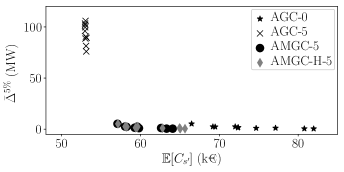
Figure 2: Expected cost vs. the average deviation of the %5 scenarios with the largest deviations.

To conclude this case study, we provide the average computational times of the different approaches. Since AGC-0 is formulated as a linear programming problem, it takes 6.1s on average to be solved. Using the efficient solution procedure proposed in [30], AGC-5 is solved in 14.3s. Since the proposed AMGC-5 requires the use of extra variables to properly model the deployment of manual reserves, its average computational time increases up to 4648s. Nevertheless, the heuristic procedure described in Section III is able to reduce this time to 60s with a very slight impact on the performance of AMGC-5.

VI Conclusions

Existing approaches to solve the stochastic OPF are either overly conservative and expensive, or leave the system vulnerable to low probability, high impact events. To address this issue, we present a novel stochastic optimal power flow formulation that distinguishes between “normal” operation conditions in which power deviations are balanced with AGC only, and “adverse” operation under which manual re-dispatch actions are required. As a result, our approach yields solutions that are more reliable and less conservative than existing approaches in the literature.

Our model is formulated as a joint chance-constraint program that limits the probability that operators manually adjust the power output of the generators. To assess the contributions of our proposal, we compare it with existing approaches using an illustrative 3-bus network and a more realistic 118-bus system. The obtained results for the larger system demonstrate that the proposed methodology is able to yield dispatch decisions that maintain almost identical security levels, but are 18% cheaper than approaches that pursue feasibility with AGC actions only under any uncertainty realization. As a counterpart, the computational burden of the proposed approach increases due to the modeling of the manual re-dispatch actions. However, we also suggest an heuristic algorithm to solve the proposed model and verify that the computational time is drastically shortened without causing a significant decline in performance.

References

- [1] J. Carpentier, “Optimal power flows,” International Journal of Electrical Power & Energy Systems, vol. 1, no. 1, pp. 3–15, 1979.
- [2] B. Stott and O. Alsaç, “Optimal power flow: Basic requirements for real-life problems and their solutions,” in SEPOPE XII Symposium, Rio de Janeiro, Brazil, vol. 11, pp. 1–10, 2012.
- [3] M. Shahidehpour, H. Yamin, and Z. Li, Market operations in electric power systems: forecasting, scheduling, and risk management. John Wiley & Sons, 2003.
- [4] S. Frank, I. Steponavice, and S. Rebennack, “Optimal power flow: A bibliographic survey I,” Energy Systems, vol. 3, no. 3, pp. 221–258, 2012.
- [5] L. Xie, P. M. Carvalho, L. A. Ferreira, J. Liu, B. H. Krogh, N. Popli, and M. D. Ilić, “Wind integration in power systems: Operational challenges and possible solutions,” Proceedings of the IEEE, vol. 99, no. 1, pp. 214–232, 2010.
- [6] L. A. Roald, D. Pozo, A. Papavasiliou, D. K. Molzahn, J. Kazempour, and A. Conejo, “Power systems optimization under uncertainty: A review of methods and applications,” Electric Power Systems Research, vol. 214, p. 108725, 2023.
- [7] J. M. Morales, A. J. Conejo, and J. Perez-Ruiz, “Economic valuation of reserves in power systems with high penetration of wind power,” IEEE Transactions on Power Systems, vol. 24, no. 2, pp. 900–910, 2009.
- [8] R. A. Jabr, S. Karaki, and J. A. Korbane, “Robust multi-period OPF with storage and renewables,” IEEE Transactions on Power Systems, vol. 30, no. 5, pp. 2790–2799, 2015.
- [9] J. Warrington, P. Goulart, S. Mariéthoz, and M. Morari, “Policy-based reserves for power systems,” IEEE Transactions on Power Systems, vol. 28, no. 4, pp. 4427–4437, 2013.
- [10] A. Lorca and X. A. Sun, “The adaptive robust multi-period alternating current optimal power flow problem,” IEEE Transactions on Power Systems, vol. 33, no. 2, pp. 1993–2003, 2018.
- [11] W. Van Ackooij, R. Zorgati, R. Henrion, and A. Möller, “Chance constrained programming and its applications to energy management,” Stochastic Optimization-Seeing the Optimal for the Uncertain, pp. 291–320, 2011.
- [12] M. Vrakopoulou, K. Margellos, J. Lygeros, and G. Andersson, “Probabilistic guarantees for the N-1 security of systems with wind power generation,” in Reliability and Risk Evaluation of Wind Integrated Power Systems, pp. 59–73, Springer, 2013.
- [13] L. Roald, F. Oldewurtel, T. Krause, and G. Andersson, “Analytical reformulation of security constrained optimal power flow with probabilistic constraints,” in 2013 IEEE Grenoble Conference, pp. 1–6, IEEE, 2013.
- [14] D. Bienstock, M. Chertkov, and S. Harnett, “Chance-constrained optimal power flow: Risk-aware network control under uncertainty,” SIAM Review, vol. 56, no. 3, pp. 461–495, 2014.
- [15] M. Lubin, Y. Dvorkin, and S. Backhaus, “A robust approach to chance constrained optimal power flow with renewable generation,” IEEE Transactions on Power Systems, vol. 31, no. 5, pp. 3840–3849, 2015.
- [16] A. M. Hou and L. A. Roald, “Chance constraint tuning for optimal power flow,” in 2020 International Conference on Probabilistic Methods Applied to Power Systems (PMAPS), pp. 1–6, 2020.
- [17] A. Peña-Ordieres, D. K. Molzahn, L. A. Roald, and A. Wächter, “DC optimal power flow with joint chance constraints,” IEEE Transactions on Power Systems, vol. 36, no. 1, pp. 147–158, 2021.
- [18] A. Esteban-Pérez and J. M. Morales, “Distributionally robust optimal power flow with contextual information,” European Journal of Operational Research, vol. 306, no. 3, pp. 1047–1058, 2023.
- [19] J. Warrington, P. J. Goulart, S. Mariéthoz, and M. Morari, “Robust reserve operation in power systems using affine policies,” in 2012 IEEE 51st IEEE Conference on Decision and Control (CDC), pp. 1111–1117, 2012.
- [20] North American Reliability Corporation (NERC), “Standard BAL-005 - Automatic Generation Control.” [Online]. Available: https://www.nerc.com/pa/Stand/Pages/Default.aspx, 2009.
- [21] R. Kannan, J. R. Luedtke, and L. A. Roald, “Stochastic DC optimal power flow with reserve saturation,” Electric Power Systems Research, vol. 189, p. 106566, 2020.
- [22] L. Roald, S. Misra, M. Chertkov, and G. Andersson, “Optimal power flow with weighted chance constraints and general policies for generation control,” in 2015 54th IEEE conference on decision and control (CDC), pp. 6927–6933, IEEE, 2015.
- [23] B. L. Miller and H. M. Wagner, “Chance constrained programming with joint constraints,” Operations Research, vol. 13, no. 6, pp. 930–945, 1965.
- [24] K. Margellos, V. Rostampour, M. Vrakopoulou, M. Prandini, G. Andersson, and J. Lygeros, “Stochastic unit commitment and reserve scheduling: A tractable formulation with probabilistic certificates,” in 2013 European Control Conference (ECC), pp. 2513–2518, 2013.
- [25] G. A. Hanasusanto, V. Roitch, D. Kuhn, and W. Wiesemann, “Ambiguous joint chance constraints under mean and dispersion information,” Operations Research, vol. 65, no. 3, pp. 751–767, 2017.
- [26] A. Nemirovski and A. Shapiro, “Scenario approximations of chance constraints,” Probabilistic and randomized methods for design under uncertainty, pp. 3–47, 2006.
- [27] J. Luedtke, “A branch-and-cut decomposition algorithm for solving chance-constrained mathematical programs with finite support,” Mathematical Programming, vol. 146, pp. 219–244, Aug. 2014.
- [28] A. Nemirovski and A. Shapiro, “Convex approximations of chance constrained programs,” SIAM Journal on Optimization, vol. 17, no. 4, pp. 969–996, 2007.
- [29] N. Jiang and W. Xie, “ALSO-X and ALSO-X+: Better convex approximations for chance constrained programs,” Operations Research, 2022.
- [30] Á. Porras, C. Domínguez, J. M. Morales, and S. Pineda, “Tight and compact sample average approximation for joint chance constrained optimal power flow,” arXiv preprint arXiv:2205.03370, 2022.
- [31] Power Grid Lib, 2022. GitHub repository, available at: (https://github.com/power-grid-lib/pglib-opf).
- [32] L. Roald, S. Misra, M. Chertkov, S. Backhaus, and G. Andersson, “Chance constrained optimal power flow with curtailment and reserves from wind power plants,” arXiv preprint arXiv:1601.04321, 2016.
- [33] OASYS, “Data of 118-node power system,” GitHub repository (https://github.com/groupoasys/AGC_and_Manual_Reserve_CC), 2023.
- [34] Gurobi Optimization, LLC, “Gurobi Optimizer Reference Manual,” 2022.