CERN-TH-2022-108
IFIC/23-08
KA-TP-02-2023
P3H-23-013
PSI-PR-23-6 Full NLO QCD predictions for Higgs-pair production in the 2-Higgs-Doublet Model

Abstract

After the discovery of the Higgs boson in 2012 at the CERN Large Hadron Collider (LHC), the study of its properties still leaves room for an extended Higgs sector with more than one Higgs boson. 2-Higgs Doublet Models (2HDMs) are well-motivated extensions of the Standard Model (SM) with five physical Higgs bosons: two CP-even states $h$ and $H$, one CP-odd state $A$, and two charged states $H^{\pm}$. In this letter, we present the calculation of the full next-to-leading order (NLO) QCD corrections to $hH$ and $AA$ production at the LHC in the 2HDM at small values of the ratio of the vacuum expectation values, $\tan\beta$, including the exact top-mass dependence everywhere in the calculation. Using techniques applied in the NLO QCD SM Higgs pair production calculation, we present results for the total cross section as well as for the invariant Higgs-pair-mass distribution at the LHC. We also provide the top-quark scale and scheme uncertainties which are found to be sizeable.

1 Introduction

2-Higgs Doublet Models Lee (1973); Branco et al. (2012) are well motivated extensions of the SM. They belong to the simplest Higgs sector extensions of the SM that, taking into account all relevant theoretical and experimental constraints, are testable at the LHC. In their type II version they contain the Higgs sector of the Minimal Supersymmetric extension of the SM (MSSM) as a special case. Featuring five physical Higgs bosons after electroweak symmetry breaking (EWSB), they represent an ideal benchmark framework for the investigation of various possible new physics effects to be expected at the LHC in multi-Higgs boson sectors.

The neutral Higgs boson pairs of the 2HDM are dominantly produced via the loop-induced gluon-fusion process $gg\to\phi_{1}\phi_{2}$, where $\phi_{1/2}$ denote scalar or pseudoscalar Higgs bosons of the 2HDM. Only for mixed scalar+pseudoscalar Higgs production the Drell–Yan-type process $q\bar{q}\to Z^{*}\to A+h/H$ takes over the dominant role in large regions of the parameter space Dawson et al. (1998). The topic of our paper is the calculation of the full NLO QCD corrections to scalar Higgs-pair and pseudoscalar Higgs-pair production via gluon fusion within the 2HDM.

In the past the NLO QCD corrections to the gluon-fusion process $gg\to HH$ have been calculated within the SM and the MSSM in the heavy-top limit (HTL) Dawson et al. (1998). This calculation has been extended to the NNLO QCD corrections in the HTL de Florian and Mazzitelli (2013a, b); Grigo et al. (2014). Quite recently, this level has been extended to the N³LO order in the HTL Banerjee et al. (2018); Chen et al. (2020a, b); Spira (2016). On the other hand finite top mass effects beyond the HTL have turned out to be sizeable Borowka et al. (2016a, b); Baglio et al. (2019, 2020, 2021). The inclusion of the related uncertainties due to the scheme and scale dependence of the virtual top mass has been shown to be mandatory, since they dominate the intrinsic theoretical uncertainties Baglio et al. (2019, 2020, 2021). For BSM scenarios, the NLO QCD corrections to all production modes involving scalar and pseudoscalar Higgs bosons are known in the HTL Dawson et al. (1998), while partial results for the virtual corrections to pseudoscalar Higgs-pair production are known beyond NLO QCD within the HTL Bhattacharya et al. (2020).

The paper is organised as follows. In Section 2 we introduce the 2HDM and the benchmark point we have selected to obtain our numerical results, then we give a short description of the details of our calculation in Section 3. Our results for $hH$ and $AA$ production are presented in Section 4. The theoretical uncertainties are discussed in Section 5, in particular the top-quark scale and scheme uncertainties in Section 5.2. A short conclusion is given in Section 6.

2 The 2-Higgs Doublet Model

The 2HDM is obtained by extending the SM by a second Higgs doublet with the same hypercharge. We work within the 2HDM version with a softly broken $\mathbb{Z}_{2}$ symmetry under which the two Higgs doublets $\Phi_{1,2}$ behave as $\Phi_{1}\to-\Phi_{1}$ and $\Phi_{2}\to\Phi_{2}$. In terms of the two $SU(2)_{L}$ Higgs doublets with hypercharge $Y=+1$ the most general scalar potential that is invariant under the $SU(2)_{L}\times U(1)_{Y}$ gauge symmetry and that has a softly broken $\mathbb{Z}_{2}$ symmetry is given by

$$V = m_{11}^{2}|\Phi_{1}|^{2}+m_{22}^{2}|\Phi_{2}|^{2}-m_{12}^{2}(\Phi_{1}^{\dagger}\Phi_{2}+h.c.)$$ (1)

$$+\frac{\lambda_{1}}{2}(\Phi_{1}^{\dagger}\Phi_{1})^{2}+\frac{\lambda_{2}}{2}(\Phi_{2}^{\dagger}\Phi_{2})^{2}+\lambda_{3}(\Phi_{1}^{\dagger}\Phi_{1})(\Phi_{2}^{\dagger}\Phi_{2})$$

$$+\lambda_{4}(\Phi_{1}^{\dagger}\Phi_{2})(\Phi_{2}^{\dagger}\Phi_{1})+\frac{\lambda_{5}}{2}[(\Phi_{1}^{\dagger}\Phi_{2})^{2}+h.c.]\;.$$

Working in the CP-conserving 2HDM, the three mass parameters, $m_{11}$, $m_{22}$ and $m_{12}$, and the five coupling parameters $\lambda_{1}$-$\lambda_{5}$ are real. The discrete $\mathbb{Z}_{2}$ symmetry (softly broken by the term proportional to $m_{12}^{2}$) has been introduced to ensure the absence of tree-level flavour-changing neutral currents (FCNC). Extending the $\mathbb{Z}_{2}$ symmetry to the fermion sector, all families of same-charge fermions will be forced to couple to a single doublet so that tree-level FCNCs will be eliminated Branco et al. (2012); Glashow and Weinberg (1977). This implies four different types of doublet couplings to the fermions that are listed in Table 1 together with the transformation properties of the fermions. The corresponding 2HDM types are named type I, type II, lepton-specific and flipped. The resulting couplings of the fermions normalised to the SM couplings can be found in Branco et al. (2012).

Model	$u_{R}$	$d_{R}$	$e_{R}$	$Q$	$u_{R}$	$d_{R}$	$L$	$l_{R}$
type I	$\Phi_{2}$	$\Phi_{2}$	$\Phi_{2}$	$+$	$+$	$+$	$+$	$+$
type II	$\Phi_{2}$	$\Phi_{1}$	$\Phi_{1}$	$+$	$+$	$-$	$+$	$-$
flipped	$\Phi_{2}$	$\Phi_{1}$	$\Phi_{2}$	$+$	$+$	$-$	$+$	$+$
lepton-specific	$\Phi_{2}$	$\Phi_{2}$	$\Phi_{1}$	$+$	$+$	$+$	$+$	$-$

Table 1: Classification of the Yukawa types of the $\mathbb{Z}_{2}$ symmetric 2HDM. 2nd-4th columns: allowed coupling combinations of Higgs doublet and fermion types; last five columns: $\mathbb{Z}_{2}$ assignments for the quark doublet $Q$, the up-type quark singlet $u_{R}$, the down-type quark singlet $d_{R}$, the lepton doublet $L$, and the lepton singlet $l_{R}$.

After EWSB, the Higgs doublets $\Phi_{i}$ $(i=1,2)$ can be expressed in terms of their vacuum expectation values (VEV) $v_{i}$, the charged complex fields $\phi_{i}^{+}$, and the real neutral CP-even and CP-odd fields $\rho_{i}$ and $\eta_{i}$, respectively, as

$$\Phi_{1}=\left(\begin{array}[]{c}\phi_{1}^{+}\\ \frac{\rho_{1}+i\eta_{1}+v_{1}}{\sqrt{2}}\end{array}\right)\qquad\mbox{and}\qquad\Phi_{2}=\left(\begin{array}[]{c}\phi_{2}^{+}\\ \frac{\rho_{2}+i\eta_{2}+v_{2}}{\sqrt{2}}\end{array}\right)\;.$$ (6)

The mass matrices are obtained from the terms bilinear in the Higgs fields in the potential. Due to charge and CP conservation they decompose into $2\times 2$ matrices ${\cal M}_{S}$, ${\cal M}_{P}$ and ${\cal M}_{C}$ for the neutral CP-even, neutral CP-odd and charged Higgs sector. They are diagonalised by the following orthogonal transformations

$$\left(\begin{array}[]{c}\rho_{1}\\ \rho_{2}\end{array}\right) = R(\alpha)\left(\begin{array}[]{c}H\\ h\end{array}\right)\;,$$ (11)

$$\left(\begin{array}[]{c}\eta_{1}\\ \eta_{2}\end{array}\right) = R(\beta)\left(\begin{array}[]{c}G^{0}\\ A\end{array}\right)\;,$$ (16)

$$\left(\begin{array}[]{c}\phi_{1}^{\pm}\\ \phi^{\pm}_{2}\end{array}\right) = R(\beta)\left(\begin{array}[]{c}G^{\pm}\\ H^{\pm}\end{array}\right)\;.$$ (21)

This leads to the physical Higgs states, a neutral light CP-even, $h$, a neutral heavy CP-even, $H$, a neutral CP-odd, $A$, and two charged Higgs bosons, $H^{\pm}$. By definition, $m_{h}<m_{H}$. The massless pseudo-Nambu-Goldstone bosons $G^{\pm}$ and $G^{0}$ are absorbed by the longitudinal components of the massive gauge bosons, the charged $W^{\pm}$ and the $Z$ boson, respectively. The rotation matrices are given in terms of the mixing angles $\vartheta=\alpha$ and $\beta$, respectively, and read

$$R(\vartheta)=\left(\begin{array}[]{cc}\cos\vartheta&-\sin\vartheta\\ \sin\vartheta&\cos\vartheta\end{array}\right)\;.$$ (24)

The mixing angle $\beta$ is related to the two VEVs as

$$\tan\beta=\frac{v_{2}}{v_{1}}\;,$$ (25)

with $v_{1}^{2}+v_{2}^{2}=v^{2}=1/(\sqrt{2}G_{F})\approx(246\mbox{ GeV})^{2}$. The mixing angle $\alpha$ is given by

$$\tan 2\alpha=\frac{2({\cal M}_{S})_{12}}{({\cal M}_{S})_{11}-({\cal M}_{S})_{22}}\;,$$ (26)

where $({\cal M}_{S})_{ij}$ ($i,j=1,2$) denote the matrix elements of the neutral CP-even scalar mass matrix ${\cal M}_{S}$. Introducing

$$M^{2}\equiv\frac{m_{12}^{2}}{s_{\beta}c_{\beta}}$$ (27)

we obtain Kanemura et al. (2004)

$$\tan 2\alpha=\frac{s_{2\beta}(M^{2}-\lambda_{345}v^{2})}{c_{\beta}^{2}(M^{2}-\lambda_{1}v^{2})-s_{\beta}^{2}(M^{2}-\lambda_{2}v^{2})}\;,$$ (28)

in terms of the abbreviation

$$\lambda_{345}\equiv\lambda_{3}+\lambda_{4}+\lambda_{5}$$ (29)

and using the short-hand notation $s_{x}\equiv\sin x$ etc.

In the minimum of the potential, the following conditions have to be fulfilled,

$$\left\langle\frac{\partial V}{\partial\Phi_{1}}\right\rangle=\left\langle\frac{\partial V}{\partial\Phi_{2}}\right\rangle=0\;,$$ (30)

where the brackets denote the vacuum expectation values. This results in the two equations

$$m_{11}^{2} = m_{12}^{2}\frac{v_{2}}{v_{1}}-\frac{\lambda_{1}v_{1}^{2}}{2}-\frac{\lambda_{345}v_{2}^{2}}{2}\;,$$ (31)

$$m_{22}^{2} = m_{12}^{2}\frac{v_{1}}{v_{2}}-\frac{\lambda_{2}v_{2}^{2}}{2}-\frac{\lambda_{345}v_{1}^{2}}{2}\;.$$ (32)

Exploiting the minimum conditions of the potential, we use the following set of independent input parameters of the model,

$$m_{h},\;m_{H},\;m_{A},\;m_{H^{\pm}},\;m_{12}^{2},\;\alpha,\;\tan\beta,\;v\;.$$ (33)

In this work we choose a benchmark point of the 2HDM type I, in which the couplings of the two Higgs doublets to the up- and down-type fermions are equal. The benchmark point of the 2HDM type I that we use in our numerical analysis is given by the following set of input parameters

$$\begin{array}[]{lcllcl}m_{h}&=&125.09\mbox{ GeV},&m_{H}&=&134.817\mbox{ GeV},\\ m_{A}&=&134.711\mbox{ GeV},&m_{H^{\pm}}&=&161.5\mbox{ GeV},\\ m_{12}^{2}&=&4305\mbox{ GeV}^{2},&\alpha&=&-0.102,\\ \tan\beta&=&3.759,&v&=&246.22\mbox{ GeV}\;.\end{array}$$ (38)

It fulfils all relevant theoretical and experimental constraints. For a description of the constraints, see Ref. Abouabid et al. (2022).

3 Calculation

3.1 Partonic leading order cross section

Figure 1: Generic one-loop diagrams for LO Higgs-boson pair production via gluon fusion, $gg\to\phi_{1}\phi_{2}$, in the 2HDM type I. The contribution from triple Higgs couplings is marked in red. Note that $\phi_{1}\phi_{2}=hH$ or $AA$.

As we work in the 2HDM type I, we are dominated by the top-quark loop contributions so that we neglect the bottom-quark loops as well as light-quark loops. Note that while we work in the 2HDM type I, we could apply our approximation to the 2HDM (with natural flavour conservation) of any type as long as we work at low $\tan\beta$ values, as the top-quark Yukawa coupling is the same in all 2HDM types. In particular we could apply our approximation to the 2HDM type II and even to the MSSM as long as the squark contributions can be suppressed, which is the case for squark mass above 400 GeV Dawson et al. (1998). This is typically the case in current MSSM fits to data Athron et al. (2017a, b); Bagnaschi et al. (2018, 2019); Arbey et al. (2022). The leading-order (LO) diagrams for $hH$ and $AA$ production, as depicted in Fig. 1 include triangle diagrams, involving a light and heavy CP-even Higgs $h,H$ propagator coupled to the final-state Higgs bosons with various triple Higgs couplings, and box diagrams with two Yukawa couplings. Note, that we focus here on the production of a mixed CP-even and a pure CP-odd Higgs pair. The analytical results and the numerical method for LO and NLO QCD $hh$ and $HH$ production can be derived from the SM results Glover and van der Bij (1988); Plehn et al. (1996); Borowka et al. (2016a, b); Baglio et al. (2019, 2020) by simple adjustments of the involved Yukawa and trilinear Higgs self-couplings as well as the sum over Higgs-boson propagators. It should be noted that for larger Higgs masses, as e.g. for $HH$ production, the top-mass effects and the associated mass and scheme uncertainties will be larger than for an SM Higgs mass of 125 GeV.

We follow the conventions of Ref. Dawson et al. (1998) and decompose the cross section into scalar form factors after the application of two tensor projectors on the matrix elements. The partonic cross section $\hat{\sigma}(gg\to\phi_{1}\phi_{2})$, with $\phi_{1}\phi_{2}=hH$ or $AA$, can be written as

$$\hat{\sigma}_{\rm LO}={\cal S}~{}\frac{G_{F}^{2}\alpha_{s}^{2}(\mu_{R}^{2})}{256\,\left(2\pi\right)^{3}}\int_{\hat{t}_{-}}^{\hat{t}^{+}}d\hat{t}\, \Big{[}\left|\left(C_{\triangle}^{h}+C_{\triangle}^{H}\right)F_{\triangle}+C_{\square}F_{\square}\right|^{2}$$

$$+\left|C_{\square}G_{\square}\right|^{2}\Big{]},$$ (39)

where $G_{F}=1.1663787\cdot 10^{-5}\,\mathrm{GeV^{-2}}$ is the Fermi constant, $\alpha_{s}(\mu_{R}^{2})$ is the strong coupling constant evaluated at the renormalisation scale $\mu_{R}$, and the Mandelstam variables $\hat{s}$ and $\hat{t}$ are given by

$$\hat{s} =Q^{2}=m_{\phi_{1}\phi_{2}}^{2},$$

$$\hat{t} =-\frac{1}{2}\left[Q^{2}-m_{\phi_{1}}^{2}-m_{\phi_{2}}^{2}-\sqrt{\lambda\left(Q^{2},m_{\phi_{1}}^{2},m_{\phi_{2}}^{2}\right)}\,\cos\theta\right],$$ (40)

with the scattering angle $\theta$ in the partonic c.m. system and where $m_{\phi_{1}}$ and $m_{\phi_{2}}$ are the Higgs boson masses, i.e. either $m_{\phi_{1}}=m_{h}$ and $m_{\phi_{2}}=m_{H}$ or $m_{\phi_{1}}=m_{\phi_{2}}=m_{A}$. The variable $m_{\phi_{1}\phi_{2}}$ denotes the invariant Higgs-pair mass. The factor ${\cal S}$ is a symmetry factor, ${\cal S}=1/2$ for $AA$ production and ${\cal S}=1$ for $hH$ production. The Källen function $\lambda$ is given by

$$\lambda(x,y,z)=(x-y-z)^{2}-4yz.$$ (41)

The integrations limits read as

$$\hat{t}_{\pm}=-\frac{1}{2}\left[Q^{2}-m_{\phi_{1}}^{2}-m_{\phi_{2}}^{2}\mp\sqrt{\lambda\left(Q^{2},m_{\phi_{1}}^{2},m_{\phi_{2}}^{2}\right)}\,\right].$$ (42)

The coefficients $C_{\triangle}^{h/H}$ contain the triple Higgs couplings$\lambda_{\phi_{1}\phi_{2}h/H}$ and the reduced Yukawa couplings $g_{h/H}^{t}$, which are given by the 2HDM Yukawa coupling modification w.r.t. to the SM top-Yukawa coupling, as well as the CP-even Higgs boson propagators,

$$C_{\triangle}^{h/H}=\lambda_{\phi_{1}\phi_{2}h/H}\,\,g_{h/H}^{t}\,\frac{v}{Q^{2}-m_{h/H}^{2}}\;.$$ (43)

The coefficient $C_{\square}$ contains only reduced Yukawa couplings to the final-state Higgs bosons,

$$C_{\square}=g_{\phi_{1}}^{t}g_{\phi_{2}}^{t}.$$ (44)

For the various $\phi_{1,2}$ they are given by

$$g_{h}^{t}=\cos\alpha/\sin\beta\,,\quad g_{H}^{t}=\sin\alpha/\sin\beta\;,\quad g_{A}^{t}=\cot\beta\;.$$ (45)

In the heavy top-limit (HTL) approximation, the form factors reduce to

$$F_{\triangle}=\frac{2}{3}\,a,\,\,\,F_{\square}=\frac{2}{3},\,\,\,G_{\square}=0,$$ (46)

with $a=-1$ for $hH$ production and $a=1$ for $AA$ production. The full $m_{t}$-dependence at LO can be found in Refs. Glover and van der Bij (1988); Plehn et al. (1996).

3.2 Hadronic cross section

The structure of the NLO QCD corrections is very similar to the SM case presented in Refs. Baglio et al. (2019, 2020). They include two-loop virtual corrections to the triangle and box diagrams, one-particle-reducible diagrams involving two triangle diagrams connected by a virtual gluon exchange, and one-loop real corrections involving an extra parton in the final state. The partonic contributions are then convolved with the parton distributions functions (PDFs) $f_{i}$ evaluated at the factorisation scale $\mu_{F}$ in order to obtain the hadronic cross section. The parton luminosities $d\mathcal{L}^{ij}/d\tau$ can be defined as

$$\frac{d\mathcal{L}^{ij}}{d\tau}=\int_{\tau}^{1}\frac{dx}{x}f_{i}\left(x,\mu_{F}\right)f_{j}\left(\frac{\tau}{x},\mu_{F}\right),$$ (47)

with $\tau=Q^{2}/s$, $s$ being the hadronic c.m. energy, so that the NLO hadronic differential cross section with respect to $Q^{2}$ can be written as

$$\frac{d\sigma_{\rm NLO}}{dQ^{2}}=\frac{d\sigma_{\rm LO}}{dQ^{2}}+\frac{d\Delta\sigma_{\rm virt}}{dQ^{2}}+\frac{d\Delta\sigma_{gg}}{dQ^{2}}+\frac{d\Delta\sigma_{qg}}{dQ^{2}}+\frac{d\Delta\sigma_{q\bar{q}}}{dQ^{2}},$$ (48)

with the LO and the virtual and real correction contributions

$$\frac{d\sigma_{\rm LO}}{dQ^{2}} =\left.\frac{d\mathcal{L}^{gg}}{d\tau}\frac{\hat{\sigma}_{\rm LO}\left(Q^{2}\right)}{s}\right|_{\tau=\frac{Q^{2}}{s}},$$

$$\frac{d\Delta\sigma_{\rm virt}}{dQ^{2}} =\left.\frac{\alpha_{s}\left(\mu_{R}^{2}\right)}{\pi}\frac{d\mathcal{L}^{gg}}{d\tau}\frac{\hat{\sigma}_{\rm LO}\left(Q^{2}\right)}{s}\,C_{\rm virt}\left(Q^{2}\right)\right|_{\tau=\frac{Q^{2}}{s}},$$

$$\frac{d\Delta\sigma_{ij}}{dQ^{2}} =\left.\frac{\alpha_{s}\left(\mu_{R}^{2}\right)}{\pi}\int_{\frac{Q^{2}}{s}}^{1}\frac{dz}{z^{2}}\frac{d\mathcal{L}^{ij}}{d\tau}\,\frac{\hat{\sigma}_{\rm LO}\left(Q^{2}\right)}{s}C_{ij}(z)\right|_{\tau=\frac{Q^{2}}{zs}},$$ (49)

for $ij=gg$, $\displaystyle\sum_{q,\bar{q}}qg$, and $\displaystyle\sum_{q}q\bar{q}$, $z=Q^{2}/\tau s$, and the variable $\tau$ is restricted to $\tau>\tau_{0}=\left(m_{\phi_{1}}+m_{\phi_{2}}\right)^{2}/s$. We include five external massless quark flavours. The coefficients $C_{virt}$ of the virtual and $C_{ij}$ of the real corrections in the HTL have been obtained in Ref. Dawson et al. (1998) and are given by

$$C_{virt} =\frac{11}{2}+\pi^{2}+C^{\infty,\,\phi_{1}\phi_{2}}_{\triangle\triangle}+\frac{33-2N_{F}}{6}\log\frac{\mu_{R}^{2}}{Q^{2}},$$

$$C_{\triangle\triangle} =$$

$$\Re e~{}\frac{\int_{\hat{t}_{-}}^{\hat{t}_{+}}d\hat{t}\left\{\left[c_{1}C_{\square}(C_{\triangle}F_{\triangle}+F_{\Box})+c_{2}\frac{p_{T}^{2}}{\hat{t}}C_{\square}^{2}G_{\Box}\right]+(\hat{t}\leftrightarrow\hat{u})\right\}}{\int_{\hat{t}_{-}}^{\hat{t}_{+}}d\hat{t}\left\{|C_{\triangle}F_{\triangle}+C_{\square}F_{\Box}|^{2}+|C_{\square}G_{\Box}|^{2}\right\}},$$

$$C^{\infty,\,hH}_{\triangle\triangle} =\left.C_{\triangle\triangle}\right|_{c_{1}=c_{2}=2/9},$$

$$C^{\infty,\,AA}_{\triangle\triangle} =\left.C_{\triangle\triangle}\right|_{c_{1}=-c_{2}=-1/2},$$

$$C_{gg} =-zP_{gg}(z)\log\frac{\mu_{F}^{2}}{\tau s}-\frac{11}{2}(1-z)^{3}$$

$$\qquad+6[1+z^{4}+(1-z)^{4}]\left(\frac{\log(1-z)}{1-z}\right)_{+},$$

$$C_{gq} =-\frac{z}{2}P_{gq}(z)\log\frac{\mu_{F}^{2}}{\tau s(1-z)^{2}}+\frac{2}{3}z^{2}-(1-z)^{2},$$

$$C_{q\bar{q}} =\frac{32}{27}(1-z)^{3},$$ (50)

where $C^{\infty,\,hH/AA}_{\triangle\triangle}$ denotes the contribution of the one-particle reducible diagrams in the HTL with the transverse momentum $p_{T}^{2}=(\hat{t}\hat{u}-m_{\phi_{1}}^{2}m_{\phi_{2}}^{2})/Q^{2}$ involving $\hat{u}=m_{\phi_{1}}^{2}+m_{\phi_{2}}^{2}-Q^{2}-\hat{t}$. The functions $P_{gg}(z)$ and $P_{gq}(z)$ are the related Altarelli-Parisi splitting kernels Altarelli and Parisi (1977), given by

$$P_{gg}(z) =6\left\{\left(\frac{1}{1-z}\right)_{+}+\frac{1}{z}-2+z(1-z)\right\}$$

$$\qquad\qquad\qquad\qquad\qquad\qquad+\frac{33-2N_{F}}{6}\delta(1-z),$$

$$P_{gq}(z) =\frac{4}{3}\frac{1+(1-z)^{2}}{z},$$ (51)

with $N_{F}=5$ in our calculation. The cross section $\hat{\sigma}_{\rm LO}(Q^{2})$ is calculated in the full theory, i.e. taking into account the finite top-quark mass at the integrand-level. The total cross section can be obtained after a final integration over $Q^{2}$ between the threshold $\left(m_{\phi_{1}}+m_{\phi_{2}}\right)^{2}$ and the hadronic c.m. energy $s$.

3.3 Virtual corrections

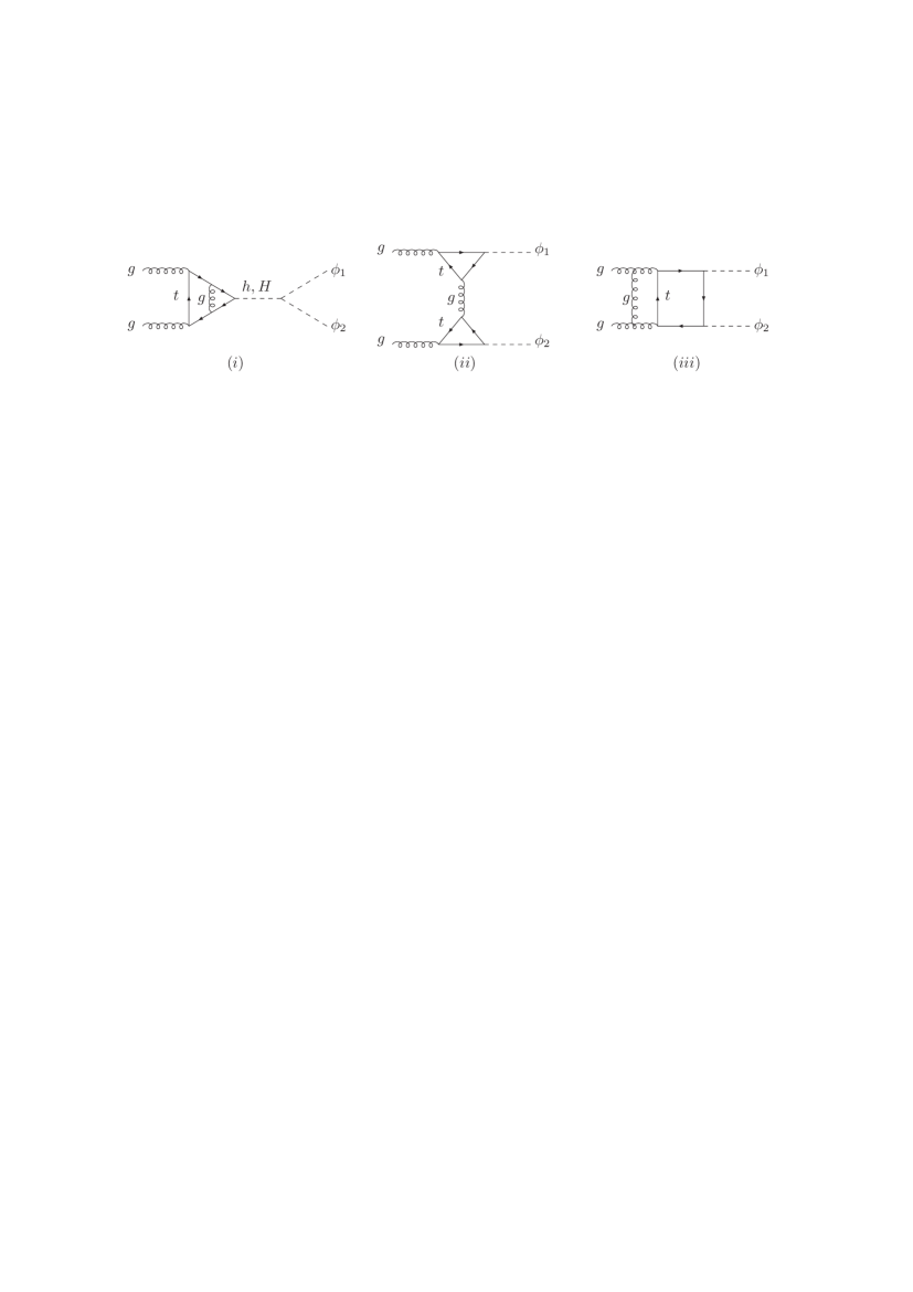
Figure 2: Generic two-loop diagrams for Higgs pair production via gluon fusion, $gg\to\phi_{1}\phi_{2}~{}(\phi_{1}\phi_{2}=hH,AA)$: (i) two-loop triangle diagrams, (ii) one-particle reducible diagrams, (iii) two-loop box diagrams.

Three generic types of diagrams contribute to the virtual corrections cf. Fig. 2: (i) two-loop triangle diagrams involving the light and heavy scalar Higgs bosons in the s-channel propagators, (ii) one-particle reducible diagrams emerging from two triangular top loops coupling to a single external Higgs boson that are connected by t-channel gluon exchange and (iii) two-loop box diagrams. The diagrams of class (i) consist of off-shell single scalar Higgs production dressed with the trilinear Higgs vertex. The relative QCD corrections coincide with the NLO QCD corrections to scalar Higgs boson production with mass $Q$ and can thus be adopted from the single-Higgs calculation Graudenz et al. (1993); Spira et al. (1995); Harlander and Kant (2005); Anastasiou et al. (2009); Aglietti et al. (2007). The diagrams of class (ii) define the coefficients $c_{1},c_{2}$ in Eq. (50). The analytical expressions of the coefficients $c_{1},c_{2}$ of the one-particle reducible contributions can be obtained from the corresponding Higgs decay widths of $\phi\to Z\gamma~{}(\phi=h,H,A)$ Cahn et al. (1979); Bergstrom and Hulth (1985); Gamberini et al. (1987) with the corresponding adjustments of the involved couplings. The full top-mass dependence of $c_{1},c_{2}$ is given by

$$c_{1} =c_{2}=2\left[I_{1}(\tau_{h},\lambda_{\hat{t}})-I_{2}(\tau_{h},\lambda_{\hat{t}})\right]$$

$$\qquad\;\;\;\;\times\left[I_{1}(\tau_{H},\lambda_{\hat{t}})-I_{2}(\tau_{H},\lambda_{\hat{t}})\right]\quad\mbox{for $\phi_{1}\phi_{2}=hH$}$$

$$c_{1} =-c_{2}=-2\left[I_{2}(\tau_{A},\lambda_{\hat{t}})\right]^{2}\qquad\qquad\mbox{for $\phi_{1}\phi_{2}=AA$}$$

$$I_{1}(\tau,\lambda) =\frac{\tau\lambda}{2(\tau-\lambda)}+\frac{\tau^{2}\lambda^{2}}{2(\tau-\lambda)^{2}}\left[f(\tau)-f(\lambda)\right]$$

$$\qquad+\frac{\tau^{2}\lambda}{(\tau-\lambda)^{2}}\left[g(\tau)-g(\lambda)\right],$$

$$I_{2}(\tau,\lambda) =-\frac{\tau\lambda}{2(\tau-\lambda)}\left[f(\tau)-f(\lambda)\right]$$ (52)

with $\tau_{\phi}=4m_{t}^{2}/m_{\phi}^{2}~{}(\phi=h,H,A)$ and $\lambda_{\hat{t}}=4m_{t}^{2}/\hat{t}$. The generic loop functions are given by

$$f(\tau) =\left\{\begin{array}[]{ll}\displaystyle\arcsin^{2}\frac{1}{\sqrt{\tau}}&\tau\geq 1\\ \displaystyle-\frac{1}{4}\left[\log\frac{1+\sqrt{1-\tau}}{1-\sqrt{1-\tau}}-i\pi\right]^{2}&\tau<1\end{array}\right.$$ (55)

$$g(\tau) =\left\{\begin{array}[]{ll}\displaystyle\sqrt{\tau-1}~{}\arcsin\frac{1}{\sqrt{\tau}}&\tau\geq 1\\ \displaystyle\frac{\sqrt{1-\tau}}{2}\left[\log\frac{1+\sqrt{1-\tau}}{1-\sqrt{1-\tau}}-i\pi\right]&\tau<1\end{array}\right.$$ (58)

These expressions approach the HTL values given in Eq. (50).

The involved part of our calculation is the two-loop box diagrams of type (iii). We have used the same method as in Refs. Baglio et al. (2019, 2020, 2021), i.e. we have performed a Feynman parametrisation, end-point subtractions and the subtraction of special infrared terms to allow for a clean separation of the ultraviolet and infrared singularities. For the stabilisation of the 6-dimensional Feynman integrals we have applied integrations by parts to reduce the powers of the singular denominators and performed the integrations with a small imaginary part of the virtual top mass. In order to arrive at the narrow-width approximation for the virtual top mass, we have used Richardson extrapolations Richardson (1911) along the lines of our SM calculation of Refs. Baglio et al. (2019, 2020). However, here we needed to extend the calculation for scalar Higgs-boson pairs to the case of different final-state Higgs masses. For the calculation of pseudoscalar Higgs-boson pairs, we have used a naive anti-commuting $\gamma_{5}$ matrix at the pseudoscalar vertices, since only even numbers of $\gamma_{5}$ contribute to the (${\cal CP}$-even) virtual corrections diagram by diagram. For this case, we have used the same projectors as in the double-scalar case, since the contributing tensor structures are the same. Since each individual two-loop box diagram is singular for the $\hat{t}$ integration, we have applied a technical cut at the integration boundaries and included a suitable substitution to stabilise this integration for each diagram. We have checked explicitly that our results do not depend on this technical cut.

The top mass has been renormalised in both the on-shell scheme and in the $\overline{\rm MS}$ scheme. The on-shell scheme predictions are our default central predictions while the $\overline{\rm MS}$ scheme predictions are used to calculate the top-quark scale and scheme uncertainties, see below. The strong coupling constant is renormalised in the $\overline{\rm MS}$ scheme with 5 active flavours. We have obtained finite results for the virtual corrections by subtracting the HTL results as in the SM case so that we end up effectively calculating the NLO mass effects only. To obtain the final hadronic differential cross section, we have added back the HTL results calculated with HPAIR. The calculation of each two-loop box diagram has been performed independently at least twice with different Feynman parametrisations and we have obtained full agreement within the numerical precision.

3.4 Real corrections

The calculation of the finite mass effects in the real corrections, $\Delta\sigma_{ij}^{\rm mass}=\Delta\sigma_{ij}-\Delta\sigma_{ij}^{\rm HTL}$, follows closely the method described in Refs. Baglio et al. (2019, 2020) for the SM case. The HTL contributions are calculated again with the program HPAIR while the partonic mass effects are obtained as

$$d\Delta\hat{\sigma}_{ij}^{\rm mass}=d\Delta\hat{\sigma}_{ij}-d\hat{\sigma}_{\rm LO}(\tilde{p}_{i})\frac{d\Delta\hat{\sigma}_{ij}^{\rm HTL}(p_{i})}{d\hat{\sigma}_{\rm LO}^{\rm HTL}(\tilde{p}_{i})},$$ (59)

where the exact four-momenta $p_{i}$ are mapped onto LO sub-space four-momenta $\tilde{p}_{i}$ following Ref. Catani and Seymour (1997).

The HTL matrix elements have been calculated analytically, while the full one-loop matrix elements have been obtained by two different methods. They have been generated using FeynArts Hahn (2001) and FormCalc Hahn and Perez-Victoria (1999) on the one hand, and obtained analytically using FeynCalc Shtabovenko et al. (2020) on the other hand. The scalar one-loop integrals have then been calculated numerically using the library COLLIER 1.2 Denner et al. (2017). The phase-space has also been parameterised in two different ways. The two methods agree within the numerical precision.

4 Numerical results

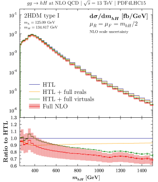
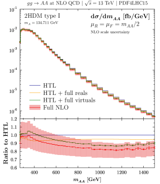
Figure 3: Invariant Higgs-pair-mass distributions for Higgs boson pair production via gluon fusion at the 13 TeV LHC as a function of $Q$ using the PDF4LHC15 PDF set, in the 2HDM type I. Left: CP-even $hH$ production. Right: CP-odd $AA$ production. In both panels, the Born-improved HTL results (in blue), HTL results including the full real corrections (in yellow), HTL results including the full virtual corrections (in green, including the numerical error), and the full NLO QCD results (in red, including the numerical error) are depicted. The inserts below display the ratio to the NLO HTL result for the different calculations. The red band indicates the renormalisation and factorisation scale uncertainties for the results including the full NLO QCD corrections.

We present our numerical results at a hadron $pp$ collider for c.m. energies of $\sqrt{s}=13$ and 14 TeV (LHC energies), $\sqrt{s}=27$ TeV (high-energy variant of the LHC, the HE-LHC), and $\sqrt{s}=100$ TeV (FCC energy). We use $m_{t}=172.5$ GeV for the on-shell top-quark mass. We have performed the calculation using the NLO PDF set PDF4LHC15 Butterworth et al. (2016) as implemented in the LHAPDF-6 library Buckley et al. (2015). Our central scale choice is $\mu_{R}=\mu_{F}=\mu_{0}=Q/2$, and $\alpha_{s}(M_{Z}^{2})$ is set according to the chosen PDF set, with an NLO running in the five-flavour scheme. As done also in the SM calculation Baglio et al. (2019, 2020), we have used the narrow-width approximation for the top quark. We use the 2HDM benchmark scenario given in Eq. (38).

We have calculated a grid of $Q$-values from $Q=259.907$ $(269.422)~{}\mathrm{GeV}$, for $hH$ production (for $AA$ production), to $Q=1500~{}\mathrm{GeV}$, so that we obtain the invariant Higgs-pair-mass distributions depicted in Fig. 3 for $hH$ production (left) and $AA$ production (right), for the LHC at 13 TeV. The results at 14 TeV are shown in Fig. 4, while the results for the HE-LHC are shown in Fig. 5 and the results for the FCC in Fig. 6. The full NLO QCD results are displayed in red, including the numerical errors as well as a band indicating the renormalisation and factorisation scale uncertainties obtained with a standard seven-point variation around our central scale choice (cf. Subsec. 5.1). The blue line shows the (Born-improved) HTL prediction, while the yellow line displays the HTL supplemented by the full mass effects in the real corrections only and the green line (including numerical errors) the HTL supplemented by the full mass effects in the virtual corrections only.

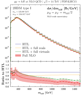
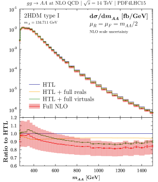
Figure 4: Same as in Fig. 3 but for $\sqrt{s}=14~{}\mathrm{TeV}$.

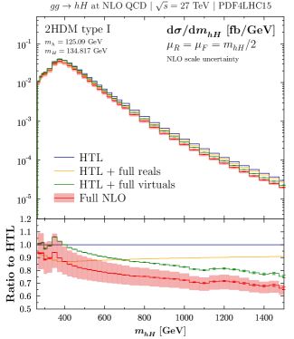
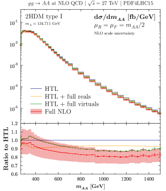
Figure 5: Same as in Fig. 3 but for $\sqrt{s}=27~{}\mathrm{TeV}$.

The mass effects in the real corrections increase with increasing c.m. energy both for $hH$ and $AA$ final states. In CP-even $hH$ production, they reach a negative peak at around $Q=400~{}\mathrm{GeV}$ and are of the order of $-10\%$ at 13 TeV (of the order of $-20\%$ at 100 TeV) before mildly increasing up to around -$6\%$ at $Q=1500~{}\mathrm{GeV}$ at 13 TeV ($-14\%$ at 100 TeV). In CP-odd $AA$ production, the behaviour of the mass effects in the real corrections is slightly different. There is also a negative peak around $Q=400~{}\mathrm{GeV}$, of the order of $-8\%$ at 13 TeV ($-14\%$ at 100 TeV), but then it mildly increases before reaching a plateau around $Q=1000~{}\mathrm{GeV}$. The mass effects are then practically constant, about $-6\%$ at 13 TeV ($-11\%$ at 100 TeV). The mass effects in the virtual corrections are negative at large $Q$ values for both $hH$ and $AA$ final states, as expected by the restoration of partial-wave unitarity in the high-energy limit. Combined with the mass effects in the real corrections, the full mass effects reach about $-30\%$ ($-40\%$) at $Q\simeq 1500~{}\mathrm{GeV}$ for $hH$ production, at lower c.m. energies (at 100 TeV), while the mass effects in the virtual corrections are smaller for $AA$ production, reaching about $-15\%$ ($-20\%$ for $Q\simeq 1500~{}\mathrm{GeV}$, at lower c.m. energies (at 100 TeV). This is the same behaviour that is observed in the SM case Borowka et al. (2016a, b); Baglio et al. (2019, 2020), albeit with a smaller correction for $AA$ production. Note that the mild increase in the mass effects in the virtual corrections at large $Q$ values for $AA$ production can be attributed to numerical fluctuations. The most striking difference between CP-even and CP-odd pair production can be seen around the $t\bar{t}$ threshold and below. There is a distortion of the shape that is distinctly different from the SM case and also between $hH$ and $AA$ productions, hence discriminating between the two production channels.

We have also obtained the total cross sections from the differential distributions, using a numerical integration of $Q$. For $Q$ between 300 GeV and 1500 GeV we have used the trapezoidal method supplemented by a Richardson extrapolation Richardson (1911) while we use a Simpson’s 3/8 rule Abramowitz and Stegun (1964) for $Q$ between 270 GeV and 300 GeV and a simple trapezoid for $Q$ between the threshold and 270 GeV. For the FCC c.m. energy of 100 TeV we have also included three new $Q$ bins between 1500 GeV and 2500 GeV and add their contribution using a Simpson’s rule. Including the numerical errors on the final decimal number, we have obtained the following results for the full NLO QCD total cross sections for $hH$ and $AA$ production in our 2HDM benchmark scenario, using PDF4LHC15 PDF sets,

$$13~{}\mathrm{TeV}:\,\,\sigma_{gg\to hH}=1.592(1)\,\mathrm{fb},\quad\sigma_{gg\to AA}=1.643(1)\,\mathrm{fb},$$

$$14~{}\mathrm{TeV}:\,\,\sigma_{gg\to hH}=1.876(1)\,\mathrm{fb},\quad\sigma_{gg\to AA}=1.927(1)\,\mathrm{fb},$$

$$27~{}\mathrm{TeV}:\,\,\sigma_{gg\to hH}=7.036(4)\,\mathrm{fb},\quad\sigma_{gg\to AA}=7.012(4)\,\mathrm{fb},$$

$$100~{}\mathrm{TeV}:\,\,\sigma_{gg\to hH}=60.49(4)\,\mathrm{fb},\quad\sigma_{gg\to AA}=58.12(3)\,\mathrm{fb}.$$ (60)

The corresponding results in the (Born-improved) HTL approximation, obtained using the same numerical integration of the $Q$ grid, are

$$13~{}\mathrm{TeV}:\,\,\sigma_{gg\to hH}^{\rm HTL}=1.793\,\mathrm{fb},\quad\sigma_{gg\to AA}^{\rm HTL}=1.717\,\mathrm{fb},$$

$$14~{}\mathrm{TeV}:\,\,\sigma_{gg\to hH}^{\rm HTL}=2.120\,\mathrm{fb},\quad\sigma_{gg\to AA}^{\rm HTL}=2.018\,\mathrm{fb},$$

$$27~{}\mathrm{TeV}:\,\,\sigma_{gg\to hH}^{\rm HTL}=8.240\,\mathrm{fb},\quad\sigma_{gg\to AA}^{\rm HTL}=7.504\,\mathrm{fb},$$

$$100~{}\mathrm{TeV}:\,\,\sigma_{gg\to hH}^{\rm HTL}=76.32\,\mathrm{fb},\quad\sigma_{gg\to AA}^{\rm HTL}=65.28\,\mathrm{fb}.$$ (61)

The comparison of Eq. (60) with Eq. (61) gives a $\simeq-12\%$ top-mass effect correction at NLO on the total cross section for $hH$ production at LHC energies ($\simeq-21\%$ at the 100 TeV FCC), and a $\simeq-5\%$ correction for $AA$ production at LHC energies ($\simeq-11\%$ at the 100 TeV FCC). While the mass effects are of similar size as the SM Higgs-pair production for CP-even Higgs bosons, they are smaller for CP-odd Higgs pair production.

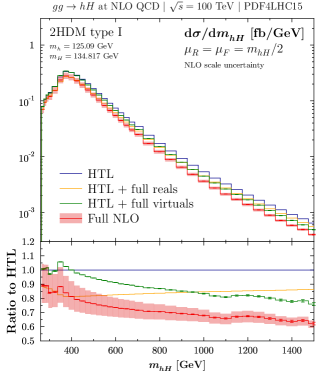
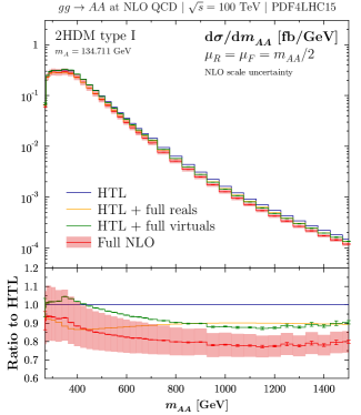
Figure 6: Same as in Fig. 3 but for $\sqrt{s}=100~{}\mathrm{TeV}$.

5 Theoretical uncertainties

5.1 Factorisation and renormalisation scale uncertainties

We have estimated the factorisation and renormalisation scale uncertainties using the standard seven-point method. We have varied both the factorisation scale $\mu_{F}$ and the renormalisation scale $\mu_{R}$ around our central scale choice $\mu_{R}=\mu_{F}=Q/2$, by a factor of two up and down while avoiding the choices leading to the ratio $\mu_{R}/\mu_{F}$ being either greater than two or smaller than one-half. The maximal and minimal cross sections obtained by this procedure are then compared to the nominal cross section obtained with the central scale choice.

We have obtained for the total cross section calculated with PDF4LHC15 parton densities the following scale uncertainties for CP-even Higgs-pair production $hH$,

$$13~{}\mathrm{TeV}:\quad\sigma_{gg\to hH}=1.592(1)^{+15.2\%}_{-13.4\%}\,\mathrm{fb},$$

$$14~{}\mathrm{TeV}:\quad\sigma_{gg\to hH}=1.876(1)^{+14.9\%}_{-13.2\%}\,\mathrm{fb},$$

$$27~{}\mathrm{TeV}:\quad\sigma_{gg\to hH}=7.036(4)^{+13.1\%}_{-11.4\%}\,\mathrm{fb},$$

$$100~{}\mathrm{TeV}:\quad\sigma_{gg\to hH}=60.49(4)^{+12.4\%}_{-10.9\%}\,\mathrm{fb},$$ (62)

while we have obtained the following results for CP-odd Higgs-pair production $AA$,

$$13~{}\mathrm{TeV}:\quad\sigma_{gg\to AA}=1.643(1)^{+17.4\%}_{-14.4\%}\,\mathrm{fb},$$

$$14~{}\mathrm{TeV}:\quad\sigma_{gg\to AA}=1.927(1)^{+17.1\%}_{-14.2\%}\,\mathrm{fb},$$

$$27~{}\mathrm{TeV}:\quad\sigma_{gg\to AA}=7.012(4)^{+15.3\%}_{-12.7\%}\,\mathrm{fb},$$

$$100~{}\mathrm{TeV}:\quad\sigma_{gg\to AA}=58.12(3)^{+15.2\%}_{-12.6\%}\,\mathrm{fb}.$$ (63)

The scale uncertainties are similar to what is obtained for SM Higgs pair production Borowka et al. (2016a, b); Baglio et al. (2019, 2020). They are slightly larger in $AA$ production than in $hH$ production. We have also found the following scale dependences for the differential cross section at 13 TeV for four distinct values of $Q$,

$$\frac{d\sigma(gg\to hH)}{dQ}\Big{|}_{Q=300~{}{\rm GeV}} =0.004278(2)^{+16.4\%}_{-13.6\%}\,\mathrm{fb/GeV},$$

$$\frac{d\sigma(gg\to hH)}{dQ}\Big{|}_{Q=400~{}{\rm GeV}} =0.007522(5)^{+15.6\%}_{-13.6\%}\,\mathrm{fb/GeV},$$

$$\frac{d\sigma(gg\to hH)}{dQ}\Big{|}_{Q=600~{}{\rm GeV}} =0.0010217(9)^{+12.1\%}_{-12.3\%}\,\mathrm{fb/GeV},$$

$$\frac{d\sigma(gg\to hH)}{dQ}\Big{|}_{Q=1200~{}{\rm GeV}} =0.00000956(6)^{+8.1\%}_{-11.3\%}\,\mathrm{fb/GeV},$$ (64)

and

$$\frac{d\sigma(gg\to AA)}{dQ}\Big{|}_{Q=300~{}{\rm GeV}} =0.01005(2)^{+18.3\%}_{-14.7\%}\,\mathrm{fb/GeV},$$

$$\frac{d\sigma(gg\to AA)}{dQ}\Big{|}_{Q=400~{}{\rm GeV}} =0.006346(6)^{+17.1\%}_{-14.4\%}\,\mathrm{fb/GeV},$$

$$\frac{d\sigma(gg\to AA)}{dQ}\Big{|}_{Q=600~{}{\rm GeV}} =0.0005328(7)^{+14.4\%}_{-13.4\%}\,\mathrm{fb/GeV},$$

$$\frac{d\sigma(gg\to AA)}{dQ}\Big{|}_{Q=1200~{}{\rm GeV}} =0.00000280(2)^{+9.7\%}_{-12.0\%}\,\mathrm{fb/GeV}.$$ (65)

5.2 Top-quark scale and scheme uncertainties

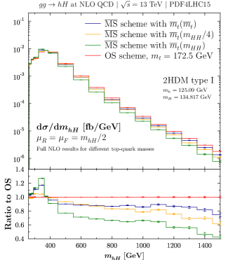
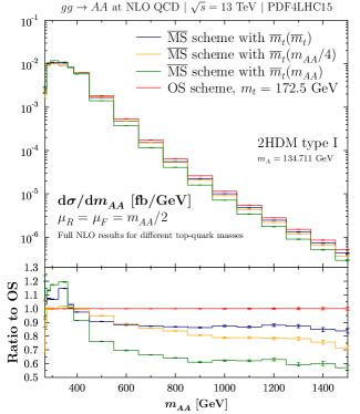
Figure 7: Higgs-pair invariant mass distribution at the 13 TeV LHC with different scale and scheme for the top-quark mass, in the 2HDM type I. Left: CP-even $hH$ production. Right: CP-odd $AA$ production. The lower panels display the ratio to the default OS prediction.

The calculation of the NLO QCD corrections has been performed in two different schemes for the renormalisation of the top-quark mass. Our central predictions use the on-shell (OS) scheme with a mass $m_{t}=172.5~{}\mathrm{GeV}$ both in the Yukawa couplings and in the loop propagators. The $\overline{\text{MS}}$ scheme can instead be used, with an appropriate choice of the top-quark mass counterterm. On top of this scheme choice, there is also a scale choice for the renormalisation of the top-quark mass, $\overline{m}(\mu_{t})$. To obtain the top-quark scale and scheme uncertainties, we have compared three $\overline{\text{MS}}$ predictions to our central OS prediction, for $\mu_{t}=Q/4$, $Q$, and $\mu_{t}$ at the $\overline{\rm MS}$ top mass itself, $\overline{m}_{t}(\overline{m}_{t})=163.02$ GeV for our choice of the OS top-quark mass value, obtained with an N³LO evolution and conversion of the pole into the $\overline{\rm MS}$ mass $\overline{m}_{t}(\overline{m}_{t})$. The minimal and maximal cross sections against the central OS prediction are used to calculate the scale and scheme uncertainties. This procedure has already been used for SM predictions and this gives rise to significant uncertainties that are comparable or even larger than the usual factorisation and renormalisation scale uncertainties Baglio et al. (2019, 2020, 2021).

We compare the five predictions (the OS predictions and the three $\overline{\text{MS}}$ predictions) in Fig. 7 at the 13 TeV LHC, in Fig. 8 at the 14 TeV LHC, in Fig. 9 at the 27 TeV HE-LHC, and in Fig. 10 at the 100 TeV FCC. The red lines display the OS full NLO QCD Higgs-pair invariant mass distributions, the blue lines the $\overline{\text{MS}}$ full NLO QCD predictions with $\overline{m}_{t}(\overline{m}_{t})$, the yellow lines the $\overline{\text{MS}}$ full NLO QCD predictions with $\overline{m}_{t}(Q/4)$, and the green lines exhibit the $\overline{\text{MS}}$ full NLO QCD predictions with $\overline{m}_{t}(Q)$. For $Q$ values above $Q=400$ GeV, the $\overline{\text{MS}}$ prediction with $\mu_{t}=Q$ always leads to the smallest distribution while the maximum at large $Q$ values is given by the OS prediction. The lower panels in each figures display the ratios of the various predictions to our central OS prediction. As in the SM case, we see large deviations at large $Q$ values, $\simeq-50\%$ at $Q=1500$ GeV for all c.m. energies. We have obtained the following uncertainties at 13 TeV for selected $Q$ values in $hH$ production using PDF4LHC15 parton densities,

$$\frac{d\sigma(gg\to hH)}{dQ}\Big{|}_{Q=300~{}{\rm GeV}} =0.004278(2)^{+13\%}_{-0\%}\,\mathrm{fb/GeV},$$

$$\frac{d\sigma(gg\to hH)}{dQ}\Big{|}_{Q=400~{}{\rm GeV}} =0.007522(5)^{+0\%}_{-9\%}\,\mathrm{fb/GeV},$$

$$\frac{d\sigma(gg\to hH)}{dQ}\Big{|}_{Q=600~{}{\rm GeV}} =0.0010217(9)^{+0\%}_{-29\%}\,\mathrm{fb/GeV},$$

$$\frac{d\sigma(gg\to hH)}{dQ}\Big{|}_{Q=1200~{}{\rm GeV}} =0.00000956(6)^{+0\%}_{-44\%}\,\mathrm{fb/GeV},$$ (66)

and the following uncertainties in $AA$ production,

$$\frac{d\sigma(gg\to AA)}{dQ}\Big{|}_{Q=300~{}{\rm GeV}} =0.01005(2)^{+17\%}_{-1\%}\,\mathrm{fb/GeV},$$

$$\frac{d\sigma(gg\to AA)}{dQ}\Big{|}_{Q=400~{}{\rm GeV}} =0.006346(6)^{+0\%}_{-9\%}\,\mathrm{fb/GeV},$$

$$\frac{d\sigma(gg\to AA)}{dQ}\Big{|}_{Q=600~{}{\rm GeV}} =0.0005328(7)^{+0\%}_{-30\%}\,\mathrm{fb/GeV},$$

$$\frac{d\sigma(gg\to AA)}{dQ}\Big{|}_{Q=1200~{}{\rm GeV}} =0.00000280(2)^{+0\%}_{-37\%}\,\mathrm{fb/GeV}.$$ (67)

As already seen in the SM case, the top-quark scale and scheme uncertainties turn out to be significant, as large or even larger than the factorisation and renormalisation scale uncertainties. For $Q>400$ GeV, the maximum cross section is always the OS prediction.

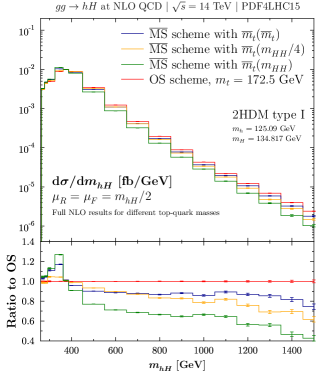
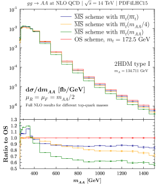
Figure 8: Same as in Fig. 7 but for $\sqrt{s}=14~{}\mathrm{TeV}$.

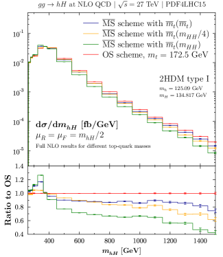
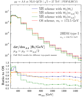
Figure 9: Same as in Fig. 7 but for $\sqrt{s}=27~{}\mathrm{TeV}$.

From the differential distributions, we can obtain the top-quark scale and scheme uncertainties on the total cross section. We adopt the envelope for each Q-bin individually to build up two maximal and minimal differential distributions and we integrate these distributions over $Q$ using fits of the various distributions which are then numerically integrated. We have arrived at the following top-quark scale and scheme uncertainties for the CP-even $hH$ total cross section,

$$13~{}\mathrm{TeV}:\quad\sigma_{gg\to hH}=1.592(1)^{+6\%}_{-11\%}\,\mathrm{fb},$$

$$14~{}\mathrm{TeV}:\quad\sigma_{gg\to hH}=1.876(1)^{+6\%}_{-11\%}\,\mathrm{fb},$$

$$27~{}\mathrm{TeV}:\quad\sigma_{gg\to hH}=7.036(4)^{+5\%}_{-12\%}\,\mathrm{fb},$$

$$100~{}\mathrm{TeV}:\quad\sigma_{gg\to hH}=60.49(4)^{+4\%}_{-14\%}\,\mathrm{fb},$$ (68)

and we have obtained the following results for the CP-odd $AA$ total cross section,

$$13~{}\mathrm{TeV}:\quad\sigma_{gg\to AA}=1.643(1)^{+9\%}_{-7\%}\,\mathrm{fb},$$

$$14~{}\mathrm{TeV}:\quad\sigma_{gg\to AA}=1.927(1)^{+9\%}_{-8\%}\,\mathrm{fb},$$

$$27~{}\mathrm{TeV}:\quad\sigma_{gg\to AA}=7.012(4)^{+8\%}_{-8\%}\,\mathrm{fb},$$

$$100~{}\mathrm{TeV}:\quad\sigma_{gg\to AA}=58.12(3)^{+7\%}_{-9\%}\,\mathrm{fb}.$$ (69)

The scale and scheme uncertainties are sizeable and should be included in an uncertainty analysis of the 2HDM Higgs-pair production cross sections according to the procedure of Ref. Baglio et al. (2021).

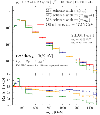
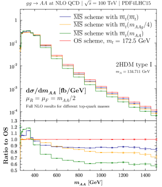
Figure 10: Same as in Fig. 7 but for $\sqrt{s}=100~{}\mathrm{TeV}$.

6 Conclusions

In this work, we have calculated the full NLO QCD corrections to mixed scalar and pure pseudoscalar Higgs-boson pair production via gluon fusion $gg\to hH,AA$ within the 2HDM type I, working in our benchmark scenario that is not excluded at the LHC. We have integrated the two-loop box diagrams numerically by performing end-point and infrared subtractions of the contributing Feynman integrals. A numerical stabilisation across the virtual thresholds has been achieved by integration by parts of the integrand to reduce the power of the problematic denominators of the Feynman integrals. The results of the triangle diagrams, involving s-channel scalar Higgs propagators and the corresponding trilinear Higgs couplings, have been adopted from the single-Higgs case. The one-particle reducible contributions emerging from either two single scalar or pseudoscalar Higgs couplings to gluons can be derived from the known results for $h,H,A\to Z\gamma$ with appropriate replacements of the contributing couplings and masses. After renormalising the top mass and the strong coupling, we have subtracted the (Born-improved) HTL to obtain the pure virtual NLO top-mass effects. The real corrections have been computed by generating the full one-loop matrix elements with automatic tools. These have then been connected to suitable subtraction matrix elements in the HTL for the radiation part, but keeping the full LO top-mass dependence. This could be achieved by suitably projected 4-momenta inside the LO sub-matrix elements. This yields the pure NLO top-mass effects of the real corrections.

Adding both subtracted virtual and real corrections, we obtain the full NLO QCD top-mass effects that have then been added to the (Born-improved) HTL results of Ref. Dawson et al. (1998) by using the code Hpair. Very similar to the corresponding SM calculation of Refs. Borowka et al. (2016a, b); Baglio et al. (2019, 2020, 2021), we find NLO top-mass effects of about 15–25% (depending on the collider energy) for the total cross sections if the top mass is defined as the top pole mass. For the invariant Higgs-pair mass distribution, the NLO top-mass effects can reach a level 30–40% for large invariant mass values. The larger the hadronic collider energy, the larger NLO top-mass effects emerge. The renormalisation and factorisation scale dependence induces uncertainties at the level of 10–15% for scalar Higgs pairs and 12–17% for pseudoscalar Higgs pairs at NLO, i.e. similar to the SM case. We have studied the additional theoretical uncertainties originating from the scale and scheme choice of the virtual top mass and obtained additional uncertainties of about 5–15% for scalar and about 10% for pseudoscalar Higgs-pair production that are significant and should be included in future Higgs-pair analyses. These uncertainties are larger for distributions at large invariant Higgs-pair masses.