On the convergence of the Willmore flow with Dirichlet boundary conditions

Abstract.

Very little is yet known regarding the Willmore flow of surfaces with Dirichlet boundary conditions. We consider surfaces with a rotational symmetry as initial data and prove a global existence and convergence result for solutions of the Willmore flow with initial data below an explicit, sharp energy threshold. Strikingly, this threshold depends on the prescribed boundary conditions — it can even be made to be $0$. We show sharpness for some critical boundary data by constructing surfaces above this energy threshold so that the corresponding Willmore flow develops a singularity. Finally, a Li-Yau inequality for open curves in $\mathbb{H}^{2}$ is proved.

1. Introduction and main results

For an immersion $f\colon\Sigma\to\operatorname{\mathbb{R}}^{3}$ of an oriented surface $\Sigma$ with boundary, one defines its Willmore energy by

(1.1) $$\mathcal{W}(f)\vcentcolon=\int_{\Sigma}H^{2}\,d\mu.$$

Here $H=\langle\vec{H},\vec{N}\rangle$ denotes the scalar mean curvature, i.e., the arithmetic mean of its principal curvatures, $\mu$ the surface measure on $\Sigma$ induced by the pull-back metric $g_{f}=f^{*}\langle\cdot,\cdot\rangle$ of the Euclidean metric in $\operatorname{\mathbb{R}}^{3}$, and $\vec{N}$ is a smooth choice of a unit normal to $f$ depending on the orientation of $\Sigma$.

Initially, the study of the Willmore energy focused mainly on closed surfaces, i.e., the case $\partial\Sigma=\emptyset$. Among compact, closed immersed surfaces in $\operatorname{\mathbb{R}}^{3}$, round spheres are the only minimizers of $\mathcal{W}$ and have energy $4\pi$. Remarkably, for such surfaces, the Willmore functional is invariant with respect to smooth conformal transformations.

Regarding the minimization of the Willmore energy among surfaces with boundary, there are several results on the existence of minimizers and critical points where different boundary conditions are prescribed, cf. [31, 7, 9, 8, 2, 15, 16, 28, 18]. In the recent contribution [25], Metsch covers the area-preserving Willmore flow with free boundary conditions. More precisely, he considers surfaces which are suitably close to a half-sphere with a small radius and which are sliding on the boundary of a domain while meeting it orthogonally.

Early work by Kuwert-Schätzle in [19] sparked great interest in the analytical properties, especially regarding long-time behavior, of the Willmore flow. Together with their results in [21] and [20], employing a suitable blow-up analysis, Kuwert-Schätzle managed to prove the following. If the initial datum $f_{0}$ is a smooth, spherical immersion (that is, $\Sigma=\mathbb{S}^{2}$) whose Willmore energy does not exceed $8\pi$, then the Willmore flow exists globally and, after suitable reparametrization, converges to a round sphere, i.e. to the global minimizer of the Willmore functional. Further, as it turns out, the energy constraint of $8\pi$ is in general sharp. Indeed, in [3], Blatt constructs spherical immersions whose Willmore energy approaches $8\pi$ arbitrarily close from above, but the Willmore flow starting in each of those immersions develops a singularity. Various numerical studies on the singular behavior of the Willmore flow are carried out in [24, 1].

In the case of immersed tori with a rotational symmetry in $\operatorname{\mathbb{R}}^{3}$, similar findings are made in [10]. As long as the Willmore energy of the initial torus does not exceed $8\pi$, Dall’Acqua-Müller-Schätzle-Spener prove global existence and convergence to the Clifford torus, the global Willmore minimizer among immersed tori. Further, they construct singular examples showing the optimality of the threshold.

The aim of this work is to give a contribution to the Willmore flow with Dirichlet boundary conditions. This being to the author’s knowledge the first work on this problem, due to its complexity, we allow ourselves to focus on a special class of initial data. This enables to go beyond perturbations of critical points of the Willmore functional.

More precisely, our analysis focuses on initial data topologically given as a cylinder $\Sigma=[0,1]\times\mathbb{S}^{1}$ with a rotational symmetry satisfying prescribed Dirichlet boundary conditions. We show global existence and convergence of solutions to the quasi-linear fourth-order Willmore boundary- and initial value problem below an explicit energy threshold that depends only on the data of the problem. Denoting by $\mathbb{H}^{2}$ the hyperbolic half-plane, by $K$ the scalar Gaussian curvature and by $\nu_{f}\colon\partial\Sigma\to\mathbb{S}^{2}$ the outward pointing unit normal field at the boundary, our main result is the following theorem.

Theorem 1.1.

Let $u_{0}\colon[0,1]\to\mathbb{H}^{2}$, $u_{0}=(u_{0}^{(1)},u_{0}^{(2)})^{t}$, denote an immersed profile curve and $f_{u_{0}}$ the associated surface of revolution on $\Sigma=[0,1]\times\mathbb{S}^{1}$, cf. (2.6). If

(1.2) $$\mathcal{W}(f_{u_{0}})\leq 4\pi-2\pi\frac{\partial_{x}u_{0}^{(2)}}{|\partial_{x}u_{0}|}\Big{|}_{0}^{1},$$

then there is a global solution $f\colon[0,\infty)\times\Sigma\to\operatorname{\mathbb{R}}^{3}$ to the Willmore flow with Dirichlet boundary conditions, i.e., to

(1.3) $$\begin{cases}\partial_{t}f=-(\Delta_{g_{f}}{H}+2{H}(H^{2}-K))\vec{N}&\text{in $[0,\infty)\times\Sigma$}\\ f(0,\cdot)=f_{u_{0}}&\text{in $\Sigma$}\\ f(t,y)=f_{u_{0}}(y)&\text{for $t\geq 0$ and $y\in\partial\Sigma$}\\ \nu_{f(t,\cdot)}(y)=\nu_{f_{u_{0}}}(y)&\text{for $t\geq 0$ and $y\in\partial\Sigma$}.\end{cases}$$

Moreover, $f(t,\cdot)$ is a surface of revolution for all $t\geq 0$ and converges up to reparametrization smoothly to a Willmore surface of revolution $f_{\infty}$ for $t\to\infty$. Lastly, $f(t,\cdot)$ for all $t\geq 0$ and $f_{\infty}$ are necessarily embedded.

We actually show global existence and convergence if one replaces (1.2) by the assumption that the hyperbolic lengths of the profile curves of $f(t,\cdot)$ remain uniformly bounded in time.

In comparison to the aforementioned results in [21, 10], the energy threshold (1.2) now depends on the Dirichlet boundary data. Strikingly, as a new feature appearing in this problem, depending on the data, it can attain any value in $[0,8\pi]$.

Knowing that, thanks to the well-posedness of the problem, solutions to (1.3) retain their rotational symmetry along the flow, we rewrite (1.3) as an evolution equation for the profile curves. The hyperbolic plane $\mathbb{H}^{2}$ naturally comes up when studying Willmore surfaces of revolution. Bryant-Griffiths found in [4] that the hyperbolic elastic energy

(1.4) $$\operatorname{\mathcal{E}}(u)\vcentcolon=\int_{I}|\vec{\kappa}|_{g}^{2}\,ds$$

where $\vec{\kappa}$ is the hyperbolic curvature, and the Willmore energy $\mathcal{W}(f_{u})$ of its surface of revolution are related by

(1.5) $$\frac{2}{\pi}\mathcal{W}(f_{u})=\operatorname{\mathcal{E}}(u)-4\frac{\partial_{x}u^{(2)}}{|\partial_{x}u|}\Big{|}_{\partial I}.$$

However, the corresponding gradient flows differ. Even though the evolution of the profile curves of surfaces evolving by Willmore flow resembles the equation for the hyperbolic elastic flow, cf. Section 2, they differ by a non-constant factor that becomes singular as the curves approach the rotation-axis, cf. [14]. Therefore, it is not clear why results on the elastic flow should aid in understanding the Willmore flow — even in the rotationally symmetric setting. The methods based on interpolation inequalities used in the study of many non-linear evolution PDEs can however be adapted to the problem. The energy threshold provides control of the singular factor. To the author’s knowledge, this is the first contribution where (1.3) is solved with an argument of this kind. In particular, the method differs from the one employed in [21, 10].

Furthermore, we construct initial data for which the Willmore flow (1.3) becomes singular. More precisely, we give a sequence of initial data satisfying fixed critical Dirichlet boundary conditions showing that (1.2) is sharp for this choice.

Theorem 1.2.

There are immersed profile curves $u_{0}^{n}\colon[0,1]\to\mathbb{H}^{2}$, $n\in\operatorname{\mathbb{N}}$, with boundary data $u_{0}^{n}(0)=u_{0}^{n}(1)=(0,1)^{t}$ and $\partial_{s}u_{0}^{n}(0)=-(0,1)^{t}$, $\partial_{s}u_{0}^{n}(1)=(0,1)^{t}$ satisfying

(1.6) $$\mathcal{W}(f_{u_{0}^{n}})\searrow 0\quad\text{for $n\to\infty$}$$

such that, for any $n\in\operatorname{\mathbb{N}}$, the maximal solution $f^{n}$ of (1.3) with $u_{0}=u_{0}^{n}$ develops a singularity. More precisely, the hyperbolic lengths of the profile curves of $f^{n}(t,\cdot)$ are unbounded in time $t$.

Since the hyperbolic length is not uniformly bounded in time, one either obtaines that the maximal existence time is finite or that reparametrizations of the solution do not converge for $t\to\infty$.

In the construction of the singular examples of Theorem 1.2, the setting of open curves introduces several difficulties compared to the case of closed curves. For instance, the singular examples constructed in [3, 26, 10] are based upon the concept of winding numbers. The winding number is constant along the flow and this fact allows to rule out all possible limits. However, for open curves, arguments based on winding numbers cannot be applied in this way. One original contribution of this work is a new argument without the aid of such topological invariants. Furthermore, understanding all potential limits is significantly more involved now that there is no closing condition.

The last statement in the formulation of Theorem 1.1 is based on a result which may be of interest by itself. Namely, we prove the following Li-Yau inequality (cf. [23]) for open curves in $\mathbb{H}^{2}$.

Theorem 1.3.

Any immersion $u\in W^{2,2}([0,1],\mathbb{H}^{2})$ with $\operatorname{\mathcal{E}}(u)\leq 8$ is an embedding.

This paper is structured as follows. In Section 2, the geometric background is developed. Firstly, the evolution equation for the profile curves is recalled. Afterwards, in Section 2.1, the singular factor in the evolution equation of the profile curves is controlled by suitable a-priori bounds for the distance of a surface of revolution to the rotation axis. Section 3 is dedicated to proving global existence of (1.3) and subconvergence. Using a Łojasiewicz-inequality for $\operatorname{\mathcal{E}}$, the subconvergence is promoted to convergence in Section 4. Section 5 is dedicated to the rigorous construction of singular examples for (1.3). To this end, various properties for segments of hyperbolic elastica which may be interesting in their own right are proved. Finally, Section 6 contains a proof of the Li-Yau inequality for open curves in $\mathbb{H}^{2}$.

2. Preliminaries

Throughout this article, we consider the half-plane model for the hyperbolic space, i.e., the Riemannian manifold $(\mathbb{H}^{2},g)$ with $\mathbb{H}^{2}\vcentcolon=\{(y^{(1)},y^{(2)})^{t}\in\operatorname{\mathbb{R}}^{2}:y^{(2)}>0\}$ and $g_{(y^{(1)},y^{(2)})}=\frac{1}{(y^{(2)})^{2}}\langle\cdot,\cdot\rangle.$ where $\langle\cdot,\cdot\rangle$ and $|\cdot|$ denote the Euclidean scalar product and norm. Given a smooth curve $u\colon I\to\mathbb{H}^{2}$ on a compact interval $I\subseteq\operatorname{\mathbb{R}}$, we define $ds\vcentcolon=ds_{u}\vcentcolon=|\partial_{x}u|_{g}dx$ and $\partial_{s}\,\cdot\vcentcolon=\partial_{s_{u}}\cdot\vcentcolon=\frac{\partial_{x}\,\cdot}{|\partial_{x}u|_{g}}$ so that $\mathcal{L}_{\mathbb{H}^{2}}(u)\vcentcolon=\int_{I}\,ds$. For a smooth vector field $X=(X^{(1)},X^{(2)})^{t}\colon I\to\operatorname{\mathbb{R}}^{2}$ along $u$,

(2.1) $$\nabla_{\partial_{x}}X=\begin{pmatrix}\partial_{x}X^{(1)}-\frac{1}{u^{(2)}}(X^{(1)}\partial_{x}u^{(2)}+X^{(2)}\partial_{x}u^{(1)})\\ \partial_{x}X^{(2)}+\frac{1}{u^{(2)}}(X^{(1)}\partial_{x}u^{(1)}-X^{(2)}\partial_{x}u^{(2)})\end{pmatrix}$$

denotes its covariant derivative in the global coordinates $(y^{(1)},y^{(2)})$ making the identification $\partial_{y^{(1)}}=(1,0)^{t}$ and $\partial_{y^{(2)}}=(0,1)^{t}$. The curvature $\vec{\kappa}$ of $u$ is

(2.2) $$\vec{\kappa}\vcentcolon=\nabla_{\partial_{s_{u}}}\partial_{s_{u}}u$$

and its elastic energy $\operatorname{\mathcal{E}}(u)\vcentcolon=\int_{I}|\vec{\kappa}|_{g}^{2}\,ds$. In order to compute the $L^{2}$-gradient, consider $U\colon(-\varepsilon,\varepsilon)\times I\to\mathbb{H}^{2}$ smooth such that each $U(t,\cdot)\colon I\to\mathbb{H}^{2}$ is an immersion and $\partial_{t}U(t,y)=0$, $\partial_{t}\partial_{s}U(t,y)=0$ for all $y\in\partial I$. Define $u\vcentcolon=U(0,\cdot)$ and $V\vcentcolon=\partial_{t}U(0,\cdot)$. As in [13, Remark 2.5], one finds

(2.3) $$\frac{d}{dt}\operatorname{\mathcal{E}}(U(t,\cdot))\Big{|}_{t=0}=\int_{I}\bigr{\langle}2(\nabla_{\partial_{s}}^{\perp})^{2}\vec{\kappa}+|\vec{\kappa}|_{g}^{2}\vec{\kappa}-2\vec{\kappa},V\bigl{\rangle}_{g}\,ds_{u}$$

where $\nabla_{\partial_{s}}^{\perp}\cdot\vcentcolon=\nabla_{\partial_{s}}\cdot\,-\,\langle\nabla_{\partial_{s}}\cdot\,,\partial_{s}u\rangle\partial_{s}u$. Therefore, we define

(2.4) $$\nabla_{L^{2}(ds_{u})}\operatorname{\mathcal{E}}(u)\vcentcolon=2(\nabla_{\partial_{s}}^{\perp})^{2}\vec{\kappa}+|\vec{\kappa}|_{g}^{2}\vec{\kappa}-2\vec{\kappa}.$$

Remark 2.1.

Clearly, $\operatorname{\mathcal{E}}$ is invariant with respect to isometries of $\mathbb{H}^{2}$. Particularly useful examples of such isometries are given by the following Möbius transformations: Identifying $\mathbb{H}^{2}$ with the subset $\{x+iy:y>0\}\subseteq\operatorname{\mathbb{C}}$

(2.5) $$\mathbb{H}^{2}\to\mathbb{H}^{2},\quad z=x+iy\mapsto\frac{az+b}{cz+d}$$

is an isometry of $\mathbb{H}^{2}$ for any $a,b,c,d\in\operatorname{\mathbb{R}}$ with $ad-bc>0$.

Furthermore, $f_{u}$ denotes the surface of revolution associated to $u$ where

(2.6) $$f_{u}\colon I\times\mathbb{S}^{1}\to\operatorname{\mathbb{R}}^{3},\quad(x,\theta)\mapsto(u^{(1)}(x),u^{(2)}(x)\cos\theta,u^{(2)}(x)\sin\theta)^{t}$$

where we identify $\mathbb{S}^{1}=\operatorname{\mathbb{R}}/(2\pi\operatorname{\mathbb{Z}})$. For the induced area measure $\mu_{f_{u}}$ on $I\times\mathbb{S}^{1}$,

(2.7) $$\mu_{f_{u}}(I\times\mathbb{S}^{1})=2\pi\int_{I}u^{(2)}|\partial_{x}u|\,dx.$$

Furthermore, if $g\colon[a,b]\to(0,\infty)$ is a smooth map and $u(x)=(x,g(x))^{t}$ for $x\in[a,b]$, one finds as in [18, Equation (2.14)] that

(2.8) $$\operatorname{\mathcal{E}}(u)=\int_{a}^{b}\frac{(\partial_{x}^{2}g(x))^{2}g(x)}{(1+(\partial_{x}g(x))^{2})^{\frac{5}{2}}}+\frac{1}{g(x)\sqrt{1+(\partial_{x}g(x))^{2}}}\,dx+2\frac{\partial_{x}g}{\sqrt{1+(\partial_{x}g)^{2}}}\Big{|}_{a}^{b}.$$

The equality in (1.5) yields that, for fixed clamped boundary data, if $f_{u}$ is a Willmore surface, then $u$ is a critical point of $\operatorname{\mathcal{E}}$. For the converse:

Lemma 2.2 ([14, Thm. 4.1]).

For a smooth immersion $u\colon I\to\mathbb{H}^{2}$, one has

(2.9) $$(\nabla_{\partial_{s}}^{\perp})^{2}\vec{\kappa}+\frac{1}{2}|\vec{\kappa}|^{2}_{g}\vec{\kappa}-\vec{\kappa}=2(u^{(2)})^{4}\left(\Delta_{g_{f_{u}}}H+2H(H^{2}-K)\right)\vec{n}$$

where $\vec{n}=\frac{1}{|\partial_{x}u|}(\partial_{x}u^{(2)},-\partial_{x}u^{(1)})^{t}$, $H$ denotes the scalar mean-curvature and $K$ the Gaussian curvature of $f_{u}$.

We obtain the following result motivating the studies of this article.

Corollary 2.3.

Consider $u\colon[0,T)\times I\to\mathbb{H}^{2}$ smooth solving

(2.10) $$\partial_{t}u=-\frac{1}{2(u^{(2)})^{4}}\bigl{(}(\nabla_{\partial_{s}}^{\perp})^{2}\vec{\kappa}+\frac{1}{2}|\vec{\kappa}|_{g}^{2}\vec{\kappa}-\vec{\kappa}\bigr{)}=-\frac{1}{4(u^{(2)})^{4}}\nabla_{L^{2}(ds_{u})}\operatorname{\mathcal{E}}(u)$$

on $[0,T)\times I$. Then $f_{u}$ solves the Willmore flow equation

(2.11) $$\partial_{t}f_{u}=-\left(\Delta_{g_{f_{u}}}H+2H(H^{2}-K)\right)\vec{N}$$

on $[0,T)\times(I\times\mathbb{S}^{1})$ where $\vec{N}=\frac{1}{|\partial_{x}u|}(\partial_{x}u^{(2)}(x),-\partial_{x}u^{(1)}(x)\cos\theta,-\partial_{x}u^{(1)}(x)\sin\theta)^{t}$.

2.1. A-priori bounds for curves with elastic energy below 8

The following result slightly generalizes the argument of [18, Lemma 4.2].

Lemma 2.4.

Consider a sequence $(u_{n})_{n\in\operatorname{\mathbb{N}}}$ of smooth, immersed curves $[0,1]\to\mathbb{H}^{2}$ such that, for $\alpha>0$, $u_{n}^{(2)}(0)\geq\alpha$ and $u_{n}^{(2)}(1)\geq\alpha$ for each $n\in\operatorname{\mathbb{N}}$. Furthermore, suppose that

(2.12) $$\sup_{n\in\operatorname{\mathbb{N}}}\operatorname{\mathcal{E}}(u_{n})<8.$$

Then there exists $c>0$ with $u_{n}^{(2)}\geq c$ for any $n\in\operatorname{\mathbb{N}}$.

Proof.

Suppose that the statement is false. That is, choosing $(x_{n})_{n\in\operatorname{\mathbb{N}}}\subseteq[0,1]$ with $u_{n}^{(2)}(x_{n})=\min_{[0,1]}u_{n}^{(2)}$, we have $u_{n}^{(2)}(x_{n})\to 0$ after passing on to a subsequence. Since $u_{n}^{(2)}(0)\geq\alpha$ and $u_{n}^{(2)}(1)\geq\alpha$, we may w.l.o.g. suppose that $u_{n}^{(2)}(x_{n})<\alpha$ and whence $x_{n}\in(0,1)$ with $\partial_{x}u_{n}^{(2)}(x_{n})=0$ for any $n\in\operatorname{\mathbb{N}}$.

Claim 1. There exist $0\leq a_{n}\leq x_{n}^{-}\leq x_{n}\leq x_{n}^{+}\leq b_{n}\leq 1$ such that

(2.13) $$\partial_{x}u_{n}^{(2)}(a_{n})\leq 0,u_{n}^{(2)}(a_{n})=\alpha\quad\text{and}\quad\partial_{x}u_{n}^{(2)}(b_{n})\geq 0,u_{n}^{(2)}(b_{n})=\alpha,$$

and

(2.14) $$\bigg{|}\frac{\partial_{x}u_{n}^{(2)}}{|\partial_{x}u_{n}|}(x_{n}^{-})\bigg{|},\bigg{|}\frac{\partial_{x}u_{n}^{(2)}}{|\partial_{x}u_{n}|}(x_{n}^{+})\bigg{|}\to 1$$

for $n\to\infty$. Notice that (2.14) and the fact that $\partial_{x}u_{n}^{(2)}(x_{n})=0$ yield $x_{n}^{-}<x_{n}<x_{n}^{+}$ for sufficiently large values of $n$.

Proof of Claim 1..

Since $u_{n}^{(2)}(x_{n})<\alpha$, setting

(2.15) $$a_{n}=\sup\{x\in[0,x_{n}]:u_{n}^{(2)}(x)\geq\alpha\}\quad\text{and}\quad b_{n}=\inf\{x\in[x_{n},1]:u_{n}^{(2)}(x)\geq\alpha\},$$

(2.13) follows. Proceeding by contradiction, suppose that no such sequence $(x_{n}^{-})$ exists. After passing to a subsequence without relabeling, we may w.l.o.g. assume

(2.16) $$\sup_{x\in[a_{n},x_{n}]}\bigg{|}\frac{\partial_{x}u_{n}^{(2)}}{|\partial_{x}u_{n}|}(x)\bigg{|}\leq 1-\delta.$$

Particularly, (2.16) yields

(2.17) $$0\leq(\partial_{x}u_{n}^{(2)})^{2}(1-(1-\delta)^{2})\leq(1-\delta)^{2}(\partial_{x}u_{n}^{(1)})^{2}.$$

Whence, since each $u_{n}$ is an immersion, it follows that $|\partial_{x}u_{n}^{(1)}|>0$ on $[a_{n},x_{n}]$ for any $n\in\operatorname{\mathbb{N}}$. Particularly, one can reparametrize $u_{n}$ as a graph on $[a_{n},x_{n}]$. Indeed, define $\varphi_{n}\colon[a_{n},x_{n}]\to[u_{n}^{(1)}(a_{n}),u_{n}^{(1)}(x_{n})]$ by $\varphi_{n}\vcentcolon=(u_{n}^{(1)})|_{[a_{n},x_{n}]}$. Since $|\partial_{x}u_{n}^{(1)}|>0$, we obtain that $\varphi_{n}$ is a diffeomorphism and $\psi_{n}\vcentcolon=\varphi_{n}^{-1}$ satisfies $\partial_{y}\psi_{n}=\frac{1}{\partial_{x}u_{n}^{(1)}\circ\psi_{n}}$. Defining $g_{n}\colon[u_{n}^{(1)}(a_{n}),u_{n}^{(1)}(x_{n})]\to(0,\infty)$ by $y\mapsto u_{n}^{(2)}\circ\psi_{n}(y)$, we have

(2.18) $$u_{n}(\psi_{n}(y))=(u_{n}^{(1)}(\psi_{n}(y)),g_{n}(y))^{t}=(y,g_{n}(y))^{t}$$

for $y\in[u_{n}^{(1)}(a_{n}),u_{n}^{(1)}(x_{n})]$. Moreover, observe that

(2.19) $$\partial_{x}u_{n}^{(1)}=\partial_{x}\varphi_{n}\quad\text{and}\quad\partial_{x}u_{n}^{(2)}=\partial_{x}(g_{n}\circ\varphi_{n})=\partial_{y}g_{n}\circ\varphi_{n}\cdot\partial_{x}\varphi_{n}.$$

Whence, (2.16) and (2.19) yield

(2.20) $$\sup_{y\in[u_{n}^{(1)}(a_{n}),u_{n}^{(1)}(x_{n})]}\bigg{|}\frac{\partial_{y}g_{n}}{\sqrt{1+(\partial_{y}g_{n})^{2}}}(y)\bigg{|}\leq 1-\delta.$$

Particularly, since $1-\delta<1$, one obtains that there exists $C>0$ with

(2.21) $$\sup_{y\in[u_{n}^{(1)}(a_{n}),u_{n}^{(1)}(x_{n})]}|\partial_{y}g_{n}(y)|\leq C\quad\text{for all }n\in\operatorname{\mathbb{N}}.$$

Using (2.8), we conclude that

(2.22) $$8 \geq\operatorname{\mathcal{E}}(u_{n})\geq\operatorname{\mathcal{E}}(u_{n}|_{[a_{n},x_{n}]})=\operatorname{\mathcal{E}}(u_{n}\circ\psi_{n}|_{[u_{n}^{(1)}(a_{n}),u_{n}^{(1)}(x_{n})]})$$

$$\underset{\eqref{eq:el-en-graphs}}{\geq}\int_{u_{n}^{(1)}(a_{n})}^{u_{n}^{(1)}(x_{n})}\frac{1}{g_{n}\sqrt{1+(\partial_{y}g_{n})^{2}}}\,dy-4=\int_{u_{n}^{(1)}(a_{n})}^{u_{n}^{(1)}(x_{n})}\frac{\sqrt{1+(\partial_{y}g_{n})^{2}}}{g_{n}\cdot(1+(\partial_{y}g_{n})^{2})}\,dy-4$$

$$\underset{\eqref{eq:bbl-4}}{\geq}\frac{1}{1+C^{2}}\cdot\bigg{|}\int_{u_{n}^{(1)}(a_{n})}^{u_{n}^{(1)}(x_{n})}\frac{\partial_{y}g_{n}}{g_{n}}\,dy\bigg{|}-4=\frac{1}{1+C^{2}}\cdot\int_{u_{n}^{(2)}(x_{n})}^{\alpha}\frac{1}{r}\,dr-4\to\infty$$

since $u_{n}^{(2)}(x_{n})\to 0$. As this is a contradiction, one obtains the existence of the sequence $(x_{n}^{-})$. Similarly, working on $[x_{n},b_{n}]$, one obtains the existence of $(x_{n}^{+})$. ∎

Consider now $n\in\operatorname{\mathbb{N}}$. Then we distinguish two cases. Firstly, suppose that $\partial_{x}u_{n}^{(2)}(x_{n}^{-})<0$. Using (1.5),

(2.23) $$\operatorname{\mathcal{E}}(u_{n}|_{[0,x_{n}]}) \geq\operatorname{\mathcal{E}}(u_{n}|_{[x_{n}^{-},x_{n}]})\underset{\eqref{eq:el-vs-will}}{=}\frac{2}{\pi}\mathcal{W}(f_{u_{n}|_{[x_{n}^{-},x_{n}]}})+4\frac{\partial_{x}u_{n}^{(2)}}{|\partial_{x}u_{n}|}\Big{|}_{x_{n}^{-}}^{x_{n}}$$

$$\geq 4\bigg{(}\frac{\partial_{x}u_{n}^{(2)}(x_{n})}{|\partial_{x}u_{n}(x_{n})|}-\frac{\partial_{x}u_{n}^{(2)}(x_{n}^{-})}{|\partial_{x}u_{n}(x_{n}^{-})|}\bigg{)}=-4\frac{\partial_{x}u_{n}^{(2)}(x_{n}^{-})}{|\partial_{x}u_{n}(x_{n}^{-})|}.$$

Secondly, if $\partial_{x}u_{n}^{(2)}(x_{n}^{-})\geq 0$, then

(2.24) $$\operatorname{\mathcal{E}}(u_{n}|_{[0,x_{n}]}) \geq\operatorname{\mathcal{E}}(u_{n}|_{[a_{n},x_{n}^{-}]})\underset{\eqref{eq:el-vs-will}}{=}\frac{2}{\pi}\mathcal{W}(f_{u_{n}|_{[a_{n},x_{n}^{-}]}})+4\frac{\partial_{x}u_{n}^{(2)}}{|\partial_{x}u_{n}|}\Big{|}_{a_{n}}^{x_{n}^{-}}$$

$$\geq 4\bigg{(}\frac{\partial_{x}u_{n}^{(2)}(x_{n}^{-})}{|\partial_{x}u_{n}(x_{n}^{-})|}-\frac{\partial_{x}u_{n}^{(2)}(a_{n})}{|\partial_{x}u_{n}(a_{n})|}\bigg{)}\underset{\eqref{eq:bbl-1}}{\geq}4\frac{\partial_{x}u_{n}^{(2)}(x_{n}^{-})}{|\partial_{x}u_{n}(x_{n}^{-})|}.$$

Using (2.14), we thus obtain that

(2.25) $$\operatorname{\mathcal{E}}(u_{n}|_{[0,x_{n}]})\geq 4+o(1).$$

Similarly, suppose that $\partial_{x}u_{n}^{(2)}(x_{n}^{+})>0$. Using (1.5),

(2.26) $$\operatorname{\mathcal{E}}(u_{n}|_{[x_{n},1]}) \geq\operatorname{\mathcal{E}}(u_{n}|_{[x_{n},x_{n}^{+}]})\underset{\eqref{eq:el-vs-will}}{=}\frac{2}{\pi}\mathcal{W}(f_{u_{n}|_{[x_{n},x_{n}^{+}]}})+4\frac{\partial_{x}u_{n}^{(2)}}{|\partial_{x}u_{n}|}\Big{|}_{x_{n}}^{x_{n}^{+}}$$

$$\geq 4\bigg{(}\frac{\partial_{x}u_{n}^{(2)}(x_{n}^{+})}{|\partial_{x}u_{n}(x_{n}^{+})|}-\frac{\partial_{x}u_{n}^{(2)}(x_{n})}{|\partial_{x}u_{n}(x_{n})|}\bigg{)}=4\frac{\partial_{x}u_{n}^{(2)}(x_{n}^{+})}{|\partial_{x}u_{n}(x_{n}^{+})|}.$$

Conversely, if $\partial_{x}u_{n}^{2}(x_{n}^{+})\leq 0$, then

(2.27) $$\operatorname{\mathcal{E}}(u_{n}|_{[x_{n},1]}) \geq\operatorname{\mathcal{E}}(u_{n}|_{[x_{n}^{+},b_{n}]})\underset{\eqref{eq:el-vs-will}}{=}\frac{2}{\pi}\mathcal{W}(f_{u_{n}|_{[x_{n}^{+},b_{n}]}})+4\frac{\partial_{x}u_{n}^{(2)}}{|\partial_{x}u_{n}|}\Big{|}_{x_{n}^{+}}^{b_{n}}$$

$$\geq 4\bigg{(}\frac{\partial_{x}u_{n}^{(2)}(b_{n})}{|\partial_{x}u_{n}(b_{n})|}-\frac{\partial_{x}u_{n}^{(2)}(x_{n}^{+})}{|\partial_{x}u_{n}(x_{n}^{+})|}\bigg{)}\underset{\eqref{eq:bbl-1}}{\geq}-4\frac{\partial_{x}u_{n}^{(2)}(x_{n}^{+})}{|\partial_{x}u_{n}(x_{n}^{+})|}.$$

Using again (2.14), we also obtain $\operatorname{\mathcal{E}}(u_{n}|_{[x_{n},1]})\geq 4+o(1)$, so together with (2.25), $\operatorname{\mathcal{E}}(u_{n})=\operatorname{\mathcal{E}}(u_{n}|_{[0,x_{n}]})+\operatorname{\mathcal{E}}(u_{n}|_{[x_{n},1]})\geq 8+o(1)$ which contradicts (2.12). ∎

Remark 2.5.

The energy bound in (2.12) is actually sharp. Indeed, for some $a>0$ and for $\varepsilon>0$ sufficiently small, consider the catenary curves $u_{\varepsilon}\colon[-a,a]\to\mathbb{H}^{2}$, $x\mapsto(x,{\varepsilon}\cdot\cosh(x/{\varepsilon}))$. Using (2.8) with $g_{\varepsilon}(x)\vcentcolon={\varepsilon}\cosh(x/{\varepsilon})$, one computes

(2.28) $$\operatorname{\mathcal{E}}(u_{\varepsilon}) =\frac{2}{{\varepsilon}}\int_{-a}^{a}\frac{1}{\cosh^{2}(x/{\varepsilon})}\,dx+2\bigg{[}\frac{\partial_{x}g_{\varepsilon}}{\sqrt{1+(\partial_{x}g_{\varepsilon})^{2}}}(a)-\frac{\partial_{x}g_{\varepsilon}}{\sqrt{1+(\partial_{x}g_{\varepsilon})^{2}}}(-a)\bigg{]}$$

$$=4\frac{e^{2a/\varepsilon}-1}{e^{2a/\varepsilon}+1}+4\tanh(a/\varepsilon)\to 8$$

for $\varepsilon\searrow 0$. Whence, $(u_{\varepsilon})_{\varepsilon>0}$ satisfy $\sup_{\varepsilon>0}\operatorname{\mathcal{E}}(u_{\varepsilon})=8$, $u_{\varepsilon}^{(2)}(\pm a)\geq\frac{3a}{2}>0$ for all $\varepsilon>0$, but $u_{\varepsilon}^{(2)}(0)=\varepsilon\to 0$. Lemma 2.4 might seem counter-intuitive since $\operatorname{\mathcal{E}}$ is invariant with respect to scaling by any parameter $\varepsilon>0$ (cf. Remark 2.1). However, the condition $\smash{u_{n}^{(2)}(0),u_{n}^{(2)}(1)\geq\alpha}$ prevents unfavorable scaling-effects.

Lemma 2.6.

Consider a sequence $(u_{n})_{n\in\operatorname{\mathbb{N}}}$ of smooth, immersed curves $[0,1]\to\mathbb{H}^{2}$ such that, for $z_{1},z_{2}\in\mathbb{H}^{2}$, $u_{n}(0)=z_{1}$ and $u_{n}(1)=z_{2}$ for each $n\in\operatorname{\mathbb{N}}$. If

(2.29) $$\sup_{n\in\operatorname{\mathbb{N}}}\operatorname{\mathcal{E}}(u_{n})<8,$$

then there exists $C>0$ with $|u_{n}|\leq C$ for any $n\in\operatorname{\mathbb{N}}$.

Proof.

Suppose that $(|u_{n}|)_{n\in\operatorname{\mathbb{N}}}$ is unbounded. As in the proof of [18, Lemma 4.3], one constructs an inversion (and thus an isometry) $R$ of the hyperbolic plane $\mathbb{H}^{2}$ such that, after passing to a subsequence, $\min_{[0,1]}(R\circ u_{n})^{(2)}\to 0$. For instance, one might choose $R(z)\vcentcolon=-\frac{1}{z}$ for $z\in\mathbb{H}^{2}\subseteq\operatorname{\mathbb{C}}$. Using Remark 2.1 and (2.29), $\sup_{n\in\operatorname{\mathbb{N}}}\operatorname{\mathcal{E}}(R\circ u_{n})<8$ and $(R\circ u_{n})(0)=R(z_{1}),\,(R\circ u_{n})(1)=R(z_{2})$ for all $n\in\operatorname{\mathbb{N}}$. By Lemma 2.4, $(R\circ u_{n})^{(2)}$ is uniformly bounded from below, a contradiction. ∎

Corollary 2.7.

Consider $p_{1},p_{2}\in\mathbb{H}^{2}$ and a subset $\mathcal{U}$ of the class of smooth immersions $[a,b]\to\mathbb{H}^{2}$ with $u(a)=p_{1}$ and $u(b)=p_{2}$ for all $u\in\mathcal{U}$. If $\sup_{u\in\mathcal{U}}\operatorname{\mathcal{E}}(u)<8$, then $\sup_{u\in\mathcal{U}}\mathcal{L}_{\mathbb{H}^{2}}(u)<\infty$.

Proof.

By Lemmata 2.4 and 2.6, there exists $K\subseteq\mathbb{H}^{2}$ compact with $u([a,b])\subseteq K$ for all $u\in\mathcal{U}$. Particularly, there exists $c>0$ with $u^{(2)}>c$ for all $u\in\mathcal{U}$.

Fix now any $u\in\mathcal{U}$. For the associated surface of revolution $f_{u}$, one has

(2.30) $$\mu_{f_{u}}([a,b]\times\mathbb{S}^{1})=2\pi\int_{I}u^{(2)}|\partial_{x}u|\,dx=2\pi\int_{I}(u^{(2)})^{2}|\partial_{x}u|_{g}\,dx\geq 2\pi c^{2}\mathcal{L}_{\mathbb{H}^{2}}(u).$$

Moreover, the area can be estimated by the Willmore energy, the diameter and a term only depending on the boundary-set $f_{u}(\{a,b\}\times\mathbb{S}^{1})$, cf. [28, bottom of p.538]. Since the diameter is controlled by $K$ and since, by (1.5), $\mathcal{W}(f_{u})\leq\frac{\pi}{2}\cdot(8+8)=8\pi$, $\sup_{u\in\mathcal{U}}\mathcal{L}_{\mathbb{H}^{2}}(u)\leq C(\frac{1}{c},K,8\pi,p_{1},p_{2})$ which concludes the proof. ∎

Remark 2.8.

Let $p\in\mathbb{H}^{2}$ and consider a subset $\mathcal{U}$ of the class of smooth immersions $[a,b]\to\mathbb{H}^{2}$ with $u(b)=p$. If $\smash{\sup_{u\in\mathcal{U}}\mathcal{L}_{\mathbb{H}^{2}}(u)<\infty}$, then there clearly exists $K\subseteq\mathbb{H}^{2}$ compact with $u([a,b])\subseteq K$ for all $u\in\mathcal{U}$.

3. Global existence and subconvergence

3.1. Evolution equations

Consider the following evolution equations of the relevant geometric quantities.

Lemma 3.1 ([13, Lemma 2.4]).

Let $u\colon[0,T)\times I\to\mathbb{H}^{2}$ be a smooth, immersed curve with $\partial_{t}u=V$ such that $\langle V,\partial_{s}u\rangle_{g}=0$. Further, consider a vector field $N\colon[0,T)\times I\to T\mathbb{H}^{2}$ which is normal to $\partial_{s}u$. Then the following formulae hold.

(3.1) $$\partial_{t}(ds_{u}) =(\partial_{s}\varphi-\langle V,\vec{\kappa}\rangle_{g})ds_{u}$$

(3.2) $$\nabla_{\partial_{s}}N =\nabla_{\partial_{s}}^{\perp}N-\langle N,\vec{\kappa}\rangle_{g}\partial_{s}u$$

(3.3) $$\nabla_{\partial_{t}}\partial_{s}u =\nabla_{\partial_{s}}^{\perp}V$$

(3.4) $$\quad(\nabla_{\partial_{t}}^{\perp}\nabla_{\partial_{s}}^{\perp}-\nabla_{\partial_{s}}^{\perp}\nabla_{\partial_{t}}^{\perp})N =\langle V,\vec{\kappa}\rangle_{g}\nabla_{\partial_{s}}^{\perp}N+\langle N,\vec{\kappa}\rangle_{g}\nabla_{\partial_{s}}^{\perp}V-\langle N,\nabla_{\partial_{s}}^{\perp}V\rangle_{g}\vec{\kappa}\qquad$$

(3.5) $$\nabla_{\partial_{t}}^{\perp}\vec{\kappa} =(\nabla_{\partial_{s}}^{\perp})^{2}V+\langle V,\vec{\kappa}\rangle_{g}\vec{\kappa}-V.$$

Notation 3.2.

Firstly, consider integers $a,b,d\in\operatorname{\mathbb{N}}_{0}$. We denote terms of type

(3.6) $$T_{u}(\partial_{s}u,\dots,\partial_{s}u,(\nabla_{\partial_{s}}^{\perp})^{i_{1}}\vec{\kappa},\dots,(\nabla_{\partial_{s}}^{\perp})^{i_{b-1}}\vec{\kappa})\cdot(\nabla_{\partial_{s}}^{\perp})^{i_{b}}\vec{\kappa}\quad\text{or}$$

(3.7) $$T_{u}(\partial_{s}u,\dots,\partial_{s}u,(\nabla_{\partial_{s}}^{\perp})^{i_{1}}\vec{\kappa},\dots,(\nabla_{\partial_{s}}^{\perp})^{i_{b}}\vec{\kappa})$$

by $P_{a}^{b,d}$ where $T$ is a smooth tensor field on $\mathbb{H}^{2}$ with $\sum_{j=1}^{b}i_{j}=a$ and $\displaystyle\max_{1\leq i\leq b}i_{j}\leq d$.

Remark 3.3.

For a particular term $P_{a}^{b,d}$ and compact $K\subseteq\mathbb{H}^{2}$ containing the trace of $u$, define

(3.8) $$C(P_{a}^{b,d},K)\vcentcolon=\max_{p\in K}\max_{\begin{subarray}{c}v_{1},v_{2},\dots\in T_{p}\mathbb{H}^{2},\\ |v_{1}|_{g},|v_{2}|_{g},\dots\leq 1\end{subarray}}T_{p}(v_{1},v_{2},\dots).$$

Writing $|x|_{g}=|x|$ with an abuse of notation for reals $x\in\operatorname{\mathbb{R}}$, one then obtains

(3.9) $$|P_{a}^{b,d}|_{g}\leq C(P_{a}^{b,d},K)\cdot|(\nabla_{\partial_{s}}^{\perp})^{i_{1}}\vec{\kappa}|_{g}\cdots|(\nabla_{\partial_{s}}^{\perp})^{i_{b}}\vec{\kappa}|_{g}.$$

Notation 3.4.

Consider integers $A,B,d\in\operatorname{\mathbb{N}}_{0}$ with $B\geq 1$. We write $\llbracket A,B\rrbracket_{d}$ for any finite sum of terms of type $P_{a}^{b,d}$ where

(3.10) $$a+\frac{b}{2}\leq A+\frac{B}{2}.$$

Example 3.5.

The requirement on $A,B$ in (3.10) describes the right algebra to apply an interpolation inequality (cf. Proposition 3.13). Moreover, the structure in (3.6) enables us to easily keep track of (derivatives of) lower-order terms in (2.10). Indeed, consider for instance

(3.11) $$-\frac{1}{2(u^{(2)})^{4}}|\vec{\kappa}|_{g}^{2}\vec{\kappa}=T_{u}(\vec{\kappa},\vec{\kappa})\vec{\kappa}=\llbracket 0,3\rrbracket_{0}$$

with $T_{(x,y)}(v_{1},v_{2})\vcentcolon=-\frac{1}{2y^{4}}\langle v_{1},v_{2}\rangle_{g}$. By differentiating, we obtain

(3.12) $$\nabla_{\partial_{s}}^{\perp}\bigg{(}-\frac{1}{2(u^{(2)})^{4}}|\vec{\kappa}|_{g}^{2}\vec{\kappa}\bigg{)}=\frac{2}{(u^{(2)})^{5}}|\kappa|_{g}^{2}\cdot\partial_{s}u^{(2)}\cdot\vec{\kappa}+2T_{u}(\nabla_{\partial_{s}}^{\perp}\vec{\kappa},\vec{\kappa})\vec{\kappa}+T(\vec{\kappa},\vec{\kappa})\nabla_{\partial_{s}}^{\perp}\vec{\kappa}.$$

The lower order terms in this computation can be efficiently taken care of by using the tensorial structure in (3.11) as in the following lemma.

Lemma 3.6.

Using Notation 3.4,

(3.13) $$\nabla_{\partial_{s}}^{\perp}\llbracket A,B\rrbracket_{d}=\llbracket A+1,B\rrbracket_{d+1}.$$

On the notation. By (3.6), $\llbracket A,B\rrbracket_{d}$ is either scalar or a vector field normal to $u$. In the scalar case, we understand that $\nabla_{\partial_{s}}^{\perp}\llbracket A,B\rrbracket_{d}\vcentcolon=\partial_{s}\llbracket A,B\rrbracket_{d}$ and proceed analogously for further directional derivatives such as $\nabla_{\partial_{t}}^{\perp}$.

Proof.

Consider any scalar term $P_{a}^{b,d}$ with $a+\frac{b}{2}\leq A+\frac{B}{2}$ given as in (3.6). Firstly,

(3.14) $$\partial_{s}T_{u}(\partial_{s}u,\dots\, ,\partial_{s}u,(\nabla_{\partial_{s}}^{\perp})^{i_{1}}\vec{\kappa},\dots,(\nabla_{\partial_{s}}^{\perp})^{i_{b}}\vec{\kappa})=(\nabla T)_{u}(\partial_{s}u,\dots,(\nabla_{\partial_{s}}^{\perp})^{i_{b}}\vec{\kappa},\partial_{s}u)$$

(3.15) $$\quad+T_{u}(\vec{\kappa},\partial_{s}u,\dots,\partial_{s}u,(\nabla_{\partial_{s}}^{\perp})^{i_{1}}\vec{\kappa},\dots,(\nabla_{\partial_{s}}^{\perp})^{i_{b}}\vec{\kappa})$$

(3.16) $$\quad+T_{u}(\partial_{s}u,\dots,\partial_{s}u,\vec{\kappa},(\nabla_{\partial_{s}}^{\perp})^{i_{1}}\vec{\kappa},\dots,(\nabla_{\partial_{s}}^{\perp})^{i_{b}}\vec{\kappa})$$

(3.17) $$\quad+T_{u}(\partial_{s}u,\dots,\partial_{s}u,\nabla_{\partial_{s}}(\nabla_{\partial_{s}}^{\perp})^{i_{1}}\vec{\kappa},\dots,(\nabla_{\partial_{s}}^{\perp})^{i_{b}}\vec{\kappa})$$

(3.18) $$\quad+T_{u}(\partial_{s}u,\dots,\partial_{s}u,(\nabla_{\partial_{s}}^{\perp})^{i_{1}}\vec{\kappa},\dots,\nabla_{\partial_{s}}(\nabla_{\partial_{s}}^{\perp})^{i_{b}}\vec{\kappa}).$$

Using (3.2), $\partial_{s}\left(T_{u}(\partial_{s}u,\dots,(\nabla_{\partial_{s}}^{\perp})^{i_{b}}\vec{\kappa})\right)=\llbracket A+1,B\rrbracket_{d+1}$ and thus (3.13). ∎

Remark 3.7.

Consider $u\colon[0,T)\times I\to M$ smooth and

(3.19) $$V=a(u)\cdot((\nabla_{\partial_{s}}^{\perp})^{2}\vec{\kappa}+\frac{1}{2}|\vec{\kappa}|_{g}^{2}\vec{\kappa}-\vec{\kappa})$$

where $a\colon\mathbb{H}^{2}\to(-\infty,0)$ is smooth. Whence, writing $a=a(u)$ for short,

(3.20) $$V =a(\nabla_{\partial_{s}}^{\perp})^{2}\vec{\kappa}+\llbracket 0,3\rrbracket_{0}=\llbracket 2,1\rrbracket_{2}\quad\text{and thus}$$

$$\nabla_{\partial_{s}}^{\perp}V =a(\nabla_{\partial_{s}}^{\perp})^{3}\vec{\kappa}+\partial_{s}a(\nabla_{\partial_{s}}^{\perp})^{2}\vec{\kappa}+\llbracket 1,3\rrbracket_{1}=\llbracket 3,1\rrbracket_{3},$$

$$(\nabla_{\partial_{s}}^{\perp})^{2}V =a(\nabla_{\partial_{s}}^{\perp})^{4}\vec{\kappa}+2\partial_{s}a(\nabla_{\partial_{s}}^{\perp})^{3}\vec{\kappa}+\llbracket 2,3\rrbracket_{2}.$$

Thus, by (3.5),

(3.21) $$\nabla_{\partial_{t}}^{\perp}\vec{\kappa}=(\nabla_{\partial_{s}}^{\perp})^{2}V+\llbracket 2,3\rrbracket_{2}=a(\nabla_{\partial_{s}}^{\perp})^{4}\vec{\kappa}+2\partial_{s}a(\nabla_{\partial_{s}}^{\perp})^{3}\vec{\kappa}+\llbracket 2,3\rrbracket_{2}=\llbracket 4,1\rrbracket_{4}.$$

Lemma 3.8.

Consider $u\colon[0,T)\times I\to\mathbb{H}^{2}$ smooth with $\partial_{t}u=a(u)\nabla_{L^{2}(ds_{u})}\operatorname{\mathcal{E}}(u)$ where $a\colon\mathbb{H}^{2}\to(-\infty,0)$ is smooth and write $\phi_{l}\vcentcolon=(\nabla_{\partial_{s}}^{\perp})^{l}\vec{\kappa}$. For any $l\in\operatorname{\mathbb{N}}_{0}$ and $k,m\in\operatorname{\mathbb{N}}$, writing $a=a(u)$ for short, we then obtain the following formulae.

(3.22) $$\nabla_{\partial_{t}}^{\perp}(\nabla_{\partial_{s}}^{\perp})^{k}\phi_{l}-(\nabla_{\partial_{s}}^{\perp})^{k}\nabla_{\partial_{t}}^{\perp}\phi_{l} =\llbracket k+l+2,3\rrbracket_{\max\{k+l,k+2\}},$$

(3.23) $$(\nabla_{\partial_{t}}^{\perp})\llbracket A,B\rrbracket_{d} =\llbracket 4+A,B\rrbracket_{4+A},$$

(3.24) $$(\nabla_{\partial_{t}}^{\perp})^{m}u-a^{m}(\nabla_{\partial_{s}}^{\perp})^{4m-2}\vec{\kappa} =2(m-1)m\cdot a^{m-1}\partial_{s}a\cdot(\nabla_{\partial_{s}}^{\perp})^{4m-3}\vec{\kappa}$$

(3.25) $$\quad+\llbracket 4m-4,3\rrbracket_{4m-4}.$$

Proof.

For (3.22), observe that, for $A\in\operatorname{\mathbb{N}}$, (3.4) yields

(3.26) $$\nabla_{\partial_{t}}^{\perp}\nabla_{\partial_{s}}^{\perp}\phi_{A}-\nabla_{\partial_{s}}^{\perp}\nabla_{\partial_{t}}^{\perp}\phi_{A} =\langle V,\vec{\kappa}\rangle_{g}\nabla_{\partial_{s}}^{\perp}\phi_{A}+\langle\phi_{A},\vec{\kappa}\rangle_{g}\nabla_{\partial_{s}}^{\perp}V-\langle\phi_{A},\nabla_{\partial_{s}}^{\perp}V\rangle_{g}\vec{\kappa}$$

$$=\llbracket A+3,3\rrbracket_{\max\{A+1,3\}}$$

using Remark 3.7. Since

(3.27) $$\nabla_{\partial_{t}}^{\perp}(\nabla_{\partial_{s}}^{\perp})^{k}\phi_{l}-(\nabla_{\partial_{s}}^{\perp})^{k}\nabla_{\partial_{t}}^{\perp}\phi_{l}=\sum_{i=0}^{k-1}(\nabla_{\partial_{s}}^{\perp})^{i}\left(\nabla_{\partial_{t}}^{\perp}\nabla_{\partial_{s}}^{\perp}\phi_{k+l-1-i}-\nabla_{\partial_{s}}^{\perp}\nabla_{\partial_{t}}^{\perp}\phi_{k+l-1-i}\right),$$

(3.22) follows. For (3.23), we firstly verify $\nabla_{\partial_{t}}^{\perp}\phi_{l}=\llbracket 4+l,1\rrbracket_{4+l}$. By (3.21), (3.22),

(3.28) $$\nabla_{\partial_{t}}^{\perp}\phi_{l} =\nabla_{\partial_{t}}^{\perp}(\nabla_{\partial_{s}}^{\perp})^{l}\vec{\kappa}=(\nabla_{\partial_{s}}^{\perp})^{l}\nabla_{\partial_{t}}^{\perp}\vec{\kappa}+\llbracket l+2,3\rrbracket_{l+2}$$

(3.29) $$=(\nabla_{\partial_{s}}^{\perp})^{l}\llbracket 4,1\rrbracket_{4}+\llbracket l+2,3\rrbracket_{l+2}=\llbracket 4+l,1\rrbracket_{4+l}.$$

Recalling the definition of $\llbracket A,B\rrbracket_{d}$, this immediately yields (3.23) with a similar argument as in the proof of Lemma 3.6 using (3.3) to deal with lower-order terms such as $\nabla_{\partial_{t}}\partial_{s}u$. Lastly, regarding (3.25), note that the case $m=1$ is a consequence of $\partial_{t}u=V$ and (3.20). Before showing the general case by induction, consider

(3.30) $$\partial_{t}a=a^{\prime}(u)\cdot\partial_{t}u=a^{\prime}(u)\cdot V=\llbracket 2,1\rrbracket_{2},$$

using (3.20), and

(3.31) $$\partial_{t}\partial_{s}a =\partial_{t}\left(a^{\prime}(u)\cdot\partial_{s}u\right)=a^{\prime\prime}(u)(\partial_{s}u,V)+a^{\prime}(u)\partial_{t}\partial_{s}u$$

$$=\llbracket 2,1\rrbracket_{2}+a^{\prime}(u)\cdot\bigl{(}\partial_{t}\left[\raise 2.15277pt\hbox{$1$}\kern-1.49994pt/\kern-0.50003pt\lower 1.07639pt\hbox{$|\partial_{x}u|_{g}$}\right]\partial_{x}u+\partial_{s}\partial_{t}u\bigr{)}$$

$$=\llbracket 2,1\rrbracket_{2}+a^{\prime}(u)\cdot\left(\langle V,\vec{\kappa}\rangle_{g}\partial_{s}u+\partial_{s}V\right)=\llbracket 3,1\rrbracket_{3},$$

using (3.20). Suppose that (3.25) holds for some $m\in\operatorname{\mathbb{N}}$. Using (3.22), (3.23),

(3.32) $$(\nabla_{\partial_{t}}^{\perp})^{m+1}u= a^{m}(\nabla_{\partial_{s}}^{\perp})^{4m-2}\nabla_{\partial_{t}}^{\perp}\vec{\kappa}$$

$$+2(m-1)m\cdot a^{m-1}\partial_{s}a\cdot(\nabla_{\partial_{s}}^{\perp})^{4m-3}\nabla_{\partial_{t}}^{\perp}\vec{\kappa}+\llbracket 4m,3\rrbracket_{4m}$$

where we also used (3.30) and (3.31) in the last equality. Using (3.21),

(3.33) $$( \nabla_{\partial_{s}}^{\perp})^{4m-2}\nabla_{\partial_{t}}^{\perp}\vec{\kappa}$$

$$=\sum_{j=0}^{4m-2}{4m-2\choose j}\left(\partial_{s}^{4m-2-j}a\cdot(\nabla_{\partial_{s}}^{\perp})^{4+j}\vec{\kappa}+2\partial_{s}^{4m-1-j}a\cdot(\nabla_{\partial_{s}}^{\perp})^{3+j}\vec{\kappa}\right)+\llbracket 4m,3\rrbracket_{4m}$$

$$=a(\nabla_{\partial_{s}}^{\perp})^{4m+2}\vec{\kappa}+((4m-2)+2)\cdot\partial_{s}a\cdot(\nabla_{\partial_{s}}^{\perp})^{4m+1}\vec{\kappa}+\llbracket 4m,3\rrbracket_{4m}$$

and similarly

(3.34) $$(\nabla_{\partial_{s}}^{\perp})^{4m-3}\nabla_{\partial_{t}}^{\perp}\vec{\kappa}=a(\nabla_{\partial_{s}}^{\perp})^{4m+1}\vec{\kappa}+\llbracket 4m,3\rrbracket_{4m}.$$

Combining, (3.32), (3.33) and (3.34) yields (3.25). ∎

Lemma 3.9.

Consider $u\colon[0,T)\times I\to\mathbb{H}^{2}$ smooth with $\partial_{t}u=\vcentcolon V$ normal to $\partial_{s}u$. Consider another normal vector field $N\colon[0,T)\times I\to T\mathbb{H}^{2}$ along $u$ and, for $a\colon\mathbb{H}^{2}\to(-\infty,0)$ smooth, define $Y\vcentcolon=\nabla_{\partial_{t}}^{\perp}N+(\nabla_{\partial_{s}}^{\perp})^{2}\left(|a(u)|\cdot(\nabla_{\partial_{s}}^{\perp})^{2}N\right)$. If $N,\nabla_{\partial_{s}}^{\perp}N=0$ on $(0,T)\times\partial I$, then

(3.35) $$\frac{d}{dt}\frac{1}{2}\int_{I}|N|_{g}^{2}\,ds+\int_{I}|a(u)|\cdot\big{|}(\nabla_{\partial_{s}}^{\perp})^{2}N\big{|}_{g}^{2}\,ds=\int_{I}\langle Y,N\rangle_{g}\,ds-\frac{1}{2}\int_{I}\left|N\right|_{g}^{2}\langle\vec{\kappa},V\rangle_{g}\,ds.$$

Proof.

The claim follows by a simple integration by parts argument. ∎

Lemma 3.10.

Under the assumptions of Lemma 3.8, it holds that $\nabla_{\partial_{s}}\vec{\kappa}=\nabla_{\partial_{s}}^{\perp}\vec{\kappa}-|\vec{\kappa}|_{g}^{2}\partial_{s}u$ and, for all $m\geq 2$,

(3.36) $$\nabla_{\partial_{s}}^{m}\vec{\kappa}=(\nabla_{\partial_{s}}^{\perp})^{m}\vec{\kappa}+\llbracket m-1,2\rrbracket_{m-1}\cdot\partial_{s}u+\llbracket m-2,3\rrbracket_{m-2}.$$

Proof.

Follows from (3.2) by induction. ∎

3.2. Global existence and subconvergence

Notation 3.11.

For a smooth immersion $u\colon I\to\mathbb{H}^{2}$, for $1\leq p<\infty$, write

(3.37) $$\|(\nabla_{\partial_{s}}^{\perp})^{j}\vec{\kappa}\|_{p}\vcentcolon=\Big{(}\int_{I}|(\nabla_{\partial_{s}}^{\perp})^{j}\vec{\kappa}|_{g}^{p}\,ds\Big{)}^{\frac{1}{p}}\quad\text{and}\quad\|(\nabla_{\partial_{s}}^{\perp})^{j}\vec{\kappa}\|_{\infty}\vcentcolon=\mathrm{sup}_{I}|(\nabla_{\partial_{s}}^{\perp})^{j}\vec{\kappa}|_{g}.$$

Then $\|\vec{\kappa}\|_{m,p}\vcentcolon=\sum_{j=0}^{m}\|(\nabla_{\partial_{s}}^{\perp})^{j}\vec{\kappa}\|_{p}$ for $p\in[1,\infty]$.

The following interpolation results will be used repeatedly.

Proposition 3.12.

Consider a smooth immersion $u\colon I\to\mathbb{H}^{2}$ with $\mathcal{L}_{\mathbb{H}^{2}}(u)>0$. Let $k\in\operatorname{\mathbb{N}}$, $p\in[2,\infty]$ and $0\leq i<k$. Then there exists $C=C(i,k,p,1/\mathcal{L}_{\mathbb{H}^{2}}(u))$ such that, writing $\alpha=(i+\frac{1}{2}-\frac{1}{p})/k$,

(3.38) $$\|(\nabla_{\partial_{s}}^{\perp})^{i}\vec{\kappa}\|_{p}\leq C\cdot\|\vec{\kappa}\|_{k,2}^{\alpha}\|\vec{\kappa}\|_{2}^{1-\alpha}.$$

Proof.

This can be proved analogously to [13, Proposition 4.1]. ∎

Proposition 3.13.

Consider a smooth immersion $u\colon I\to\mathbb{H}^{2}$ with $\mathcal{L}_{\mathbb{H}^{2}}(u)>0$. Further suppose that there exists $K\subseteq\mathbb{H}^{2}$ compact with $u(I)\subseteq K$. For any $k\in\operatorname{\mathbb{N}}$ and integers $a,b,d$ with $b\geq 2$, $d\leq k-1$ and $a+\frac{b}{2}<2k+1$, there is a constant $C$ depending only on $k$, $a$, $b$, ${1}/{\mathcal{L}_{\mathbb{H}^{2}}(u)}$ and $C(P_{a}^{b,d},K)$ from (3.8) with

(3.39) $$\int_{I}|P_{a}^{b,d}|_{g}\,ds\leq C\cdot\|\vec{\kappa}\|_{k,2}^{\gamma}\cdot\|\vec{\kappa}\|_{2}^{b-\gamma}$$

where $\gamma=(a+b/2-1)/k$. Moreover, for any $\varepsilon\in(0,1)$,

(3.40) $$\int_{I}|P_{a}^{b,d}|_{g}\,ds\leq\varepsilon\|(\nabla_{\partial_{s}}^{\perp})^{k}\vec{\kappa}\|_{2}^{2}+C\varepsilon^{-\frac{\gamma}{2-\gamma}}\|\vec{\kappa}\|_{2}^{2\frac{b-\gamma}{2-\gamma}}+C\|\vec{\kappa}\|_{2}^{b}.$$

Proof.

Using (3.9), the statement is shown just as [13, Proposition 4.3]. ∎

Theorem 3.14.

Let $u_{0}\colon I\to\mathbb{H}^{2}$ be a smooth immersion, $a\colon\mathbb{H}^{2}\to(-\infty,0)$ smooth and suppose that $u\colon[0,T)\times I\to\mathbb{H}^{2}$ is a time-maximal solution of

(3.41) $$\begin{cases}\partial_{t}u=a(u)((\nabla_{\partial_{s}}^{\perp})^{2}\vec{\kappa}+\frac{1}{2}|\vec{\kappa}|_{g}^{2}\vec{\kappa}-\vec{\kappa})&\text{on }[0,T)\times I\\ u(0,\cdot)=u_{0}&\text{on }I\\ u(t,y)=u_{0}(y)&\text{for }(t,y)\in[0,T)\times\partial I\\ \partial_{s}u(t,y)=\partial_{s}u_{0}(y)&\text{for }(t,y)\in[0,T)\times\partial I.\end{cases}$$

with

(3.42) $$\sup_{t\in[0,T)}\mathcal{L}_{\mathbb{H}^{2}}(u(t,\cdot))<\infty.$$

Then the solution exists globally in time, that is, $T=\infty$.

Remark 3.15.

With the same arguments as in [30], the existence of a time-maximal solution $u$ of (3.41) can be shown for any immersion $u_{0}\in W^{2,2}(I,\mathbb{H}^{2})$ yielding, for any $0<T^{\prime}<T$,

(3.43) $$u\in C^{\infty}((0,T),\mathbb{H}^{2})\cap W^{1,2}([0,T^{\prime}],L^{2}(I,\mathbb{H}^{2}))\cap L^{2}([0,T^{\prime}],W^{4,2}(I,\mathbb{H}^{2})).$$

Especially, $u(t,\cdot)\to u_{0}$ in $W^{2,2}(I,\mathbb{H}^{2})$ for $t\searrow 0$.

Proof of Theorem 3.14.

Firstly, note

(3.44) $$\frac{d}{dt}\operatorname{\mathcal{E}}(u(t,\cdot))=-\int_{I}|a(u)|\cdot|(\nabla_{\partial_{s}}^{\perp})^{2}\vec{\kappa}+\frac{1}{2}|\vec{\kappa}|_{g}^{2}\vec{\kappa}-\vec{\kappa}|_{g}^{2}\leq 0.$$

Moreover, by (3.42) and Remark 2.8 with $p=u_{0}(y)$ for some $y\in\partial I$, there exists a compact $K\subseteq\mathbb{H}^{2}$ with $u(t,x)\in K$ for all $t\in[0,T)$ and $x\in I$.

Secondly, we establish a lower bound on the length of each $u(t,\cdot)$. Write $I=[\alpha,\beta]$. If $u(\alpha)\neq u(\beta)$, this is clear. Next, if $u(\alpha)$ = $u(\beta)$ but $\partial_{s}u(\alpha)\neq\partial_{s}u(\beta)$, then there exists $v\in\operatorname{\mathbb{R}}^{2}$ with $|v|=1$ such that $\langle\partial_{s}u(\alpha),v\rangle_{g}\neq\langle\partial_{s}u(\beta),v\rangle_{g}$. Particularly,

(3.45) $$0< |\langle\partial_{s}u(\beta),v\rangle_{g}-\langle\partial_{s}u(\alpha),v\rangle_{g}|\leq\int_{I}|\partial_{s}\langle\partial_{s}u,v\rangle_{g}|\,ds=\int_{I}|\langle\vec{\kappa},v\rangle_{g}|\,ds$$

$$\leq(\operatorname{\mathcal{E}}(u))^{\frac{1}{2}}\cdot\bigg{(}\int_{I}\frac{1}{(u^{(2)})^{2}}\,ds\bigg{)}^{\frac{1}{2}}\leq(\operatorname{\mathcal{E}}(u_{0}))^{\frac{1}{2}}\Big{(}\mathcal{L}_{\mathbb{H}^{2}}(u)/\min_{(x,y)\in K}y^{2}\Big{)}^{\frac{1}{2}}$$

which shows boundedness of the hyperbolic length from below. Lastly, if $u(\alpha)=u(\beta)$ and $\partial_{s}u(\alpha)=\partial_{s}u(\beta)$, Fenchel’s theorem in $\mathbb{H}^{2}$ (cf. [13, Theorem 2.3]) yields

(3.46) $$2\pi\leq\int_{I}|\vec{\kappa}|_{g}\,ds\leq\sqrt{\mathcal{L}_{\mathbb{H}^{2}}(u)}\sqrt{\operatorname{\mathcal{E}}(u)}\leq\sqrt{\operatorname{\mathcal{E}}(u_{0})}\cdot\sqrt{\mathcal{L}_{\mathbb{H}^{2}}(u)}$$

and thus again boundedness of $\mathcal{L}_{\mathbb{H}^{2}}(u)$ from below. From now on, write $a=a(u)$.

Step 1: Time-uniform bounds on $\|(\nabla_{\partial_{s}}^{\perp})^{l}\vec{\kappa}\|_{2}$. Firstly, we apply Lemma 3.9 with $N=|a|^{\eta}(\nabla_{\partial_{t}}^{\perp})^{m}u$ for fixed $m\in\operatorname{\mathbb{N}}$ where $\eta\vcentcolon=-\frac{1}{2}$. Notice that $N,\nabla_{\partial_{s}}^{\perp}N=0$ on $[0,T)\times\partial I$ by the boundary conditions, cf. [11, Remark 2.5]. One obtains

(3.47) $$\frac{d}{dt}\frac{1}{2} \int_{I}|a|^{2\eta}\cdot|(\nabla_{\partial_{t}}^{\perp})^{m}u|_{g}^{2}\,ds+\int_{I}|a|\cdot|(\nabla_{\partial_{s}}^{\perp})^{2}[|a|^{\eta}(\nabla_{\partial_{t}}^{\perp})^{m}u]|_{g}^{2}\,ds$$

$$=\int_{I}\langle Y,|a|^{\eta}(\nabla_{\partial_{t}}^{\perp})^{m}u\rangle_{g}\,ds-\frac{1}{2}\int_{I}|a|^{2\eta}\cdot|(\nabla_{\partial_{t}}^{\perp})^{m}u|_{g}^{2}\langle\vec{\kappa},V\rangle_{g}\,ds$$

where

(3.48) $$Y=|a|^{\eta}(\nabla_{\partial_{t}}^{\perp})^{m+1}u+(\nabla_{\partial_{s}}^{\perp})^{2}\left[|a|\cdot(\nabla_{\partial_{s}}^{\perp})^{2}(|a|^{\eta}\cdot(\nabla_{\partial_{t}}^{\perp})^{m}u)\right]+\llbracket 4m,3\rrbracket_{4m}$$

and $V$ is as in (3.20). In computing $Y$ in (3.48), terms involving $\partial_{t}a$ contribute only to $\llbracket 4m,3\rrbracket_{4m}$, cf. (3.30). Using $|a|=-a$, we compute

(3.49) $$( \nabla_{\partial_{s}}^{\perp})^{2}\left[|a|\cdot(\nabla_{\partial_{s}}^{\perp})^{2}(|a|^{\eta}\cdot(\nabla_{\partial_{t}}^{\perp})^{m}u)\right]$$

$$=(\nabla_{\partial_{s}}^{\perp})^{2}\Bigl{[}|a|\cdot\bigl{(}|a|^{\eta}(\nabla_{\partial_{s}}^{\perp})^{2}(\nabla_{\partial_{t}}^{\perp})^{m}u-2\eta|a|^{\eta-1}\partial_{s}a\nabla_{\partial_{s}}^{\perp}(\nabla_{\partial_{t}}^{\perp})^{m}u\bigr{)}$$

$$\quad+\llbracket 4m-2,3\rrbracket_{4m-2}\Bigr{]}$$

$$=-a|a|^{\eta}(\nabla_{\partial_{s}}^{\perp})^{4}(\nabla_{\partial_{t}}^{\perp})^{m}u-2(\eta+1)|a|^{\eta}\partial_{s}a(\nabla_{\partial_{s}}^{\perp})^{3}(\nabla_{\partial_{t}}^{\perp})^{m}u$$

$$\quad-2\eta|a|^{\eta}\partial_{s}a(\nabla_{\partial_{s}}^{\perp})^{3}(\nabla_{\partial_{t}}^{\perp})^{m}u+\llbracket 4m,3\rrbracket_{4m}$$

$$=-a|a|^{\eta}(\nabla_{\partial_{s}}^{\perp})^{4}(\nabla_{\partial_{t}}^{\perp})^{m}u-2\smash{\underbrace{(2\eta+1)}_{\mathclap{=\,0\text{ by the above choice of $\eta$.}}}}|a|^{\eta}\partial_{s}a(\nabla_{\partial_{s}}^{\perp})^{3}(\nabla_{\partial_{t}}^{\perp})^{m}u+\llbracket 4m,3\rrbracket_{4m}$$

and, using (3.25),

(3.50) $$( \nabla_{\partial_{s}}^{\perp})^{4}(\nabla_{\partial_{t}}^{\perp})^{m}u$$

$$=a^{m}(\nabla_{\partial_{s}}^{\perp})^{4m+2}\vec{\kappa}+2m(m+1)a^{m-1}\partial_{s}a(\nabla_{\partial_{s}}^{\perp})^{4m+1}\vec{\kappa}+\llbracket 4m,3\rrbracket_{4m}.$$

Whence, combining (3.49) and (3.50), and observing that the terms of order $4m+2$ and $4m+1$ in $\vec{\kappa}$ cancel with the corresponding ones in $(\nabla_{\partial_{t}}^{\perp})^{m+1}u$, using (3.25) and (3.48), $Y=\llbracket 4m,3\rrbracket_{4m}$. Since we would like to apply Proposition 3.13 to the right-hand-side of (3.47) with $k=4m$, we need to make sure that there are no terms of order $4m$ to which we apply the interpolation inequality.

Claim 1. We have that

(3.51) $$\int_{I}\langle Y,|a|^{\eta}(\nabla_{\partial_{t}}^{\perp})^{m}u\rangle\,ds=\int_{I}\llbracket 8m-2,4\rrbracket_{4m-1}\,ds.$$

Proof of Claim 1..

Consider any term in $Y=\llbracket 4m,3\rrbracket_{4m}$ which contains a term $(\nabla_{\partial_{s}}^{\perp})^{4m}\vec{\kappa}$. In general, one such term is given by

(3.52) $$T_{u}(\underbrace{\partial_{s}u,\dots,\partial_{s}u}_{c\in\operatorname{\mathbb{N}}_{0}\text{-times}},\underbrace{\vec{\kappa},\dots,\vec{\kappa}}_{b\in\operatorname{\mathbb{N}}_{0}\text{-times}},(\nabla_{\partial_{s}}^{\perp})^{4m}\vec{\kappa})^{\perp}$$

where $T\in\mathcal{T}^{c+b+1}_{1}(\mathbb{H}^{2})$ is a vector-valued tensor field on $\mathbb{H}^{2}$ and

(3.53) $$4m+\frac{1}{2}(b+1)\leq 4m+\frac{3}{2}\quad\Longleftrightarrow\quad b\leq 2.$$

By the product rule for covariant differentiation of tensors and (3.2), (3.53),

(3.54) $$T(\partial_{s}u,\dots,(\nabla_{\partial_{s}}^{\perp})^{4m}\vec{\kappa})^{\perp}=\nabla_{\partial_{s}}^{\perp}\bigl{(}\smash{\underbrace{T(\partial_{s}u,\dots,(\nabla_{\partial_{s}}^{\perp})^{4m-1}\vec{\kappa})^{\perp}}_{=\,\llbracket 4m-1,3\rrbracket_{4m-1}}}\bigr{)}+\llbracket 4m,3\rrbracket_{4m-1}.$$

Whence, integration by parts yields

(3.55) $$\int_{I}\langle T(\partial_{s}u,\dots,(\nabla_{\partial_{s}}^{\perp})^{4m}\vec{\kappa})^{\perp},|a|^{\eta}(\nabla_{\partial_{t}}^{\perp})^{m}u\rangle_{g}\,ds$$

$$=\int_{I}-\langle\llbracket 4m-1,3\rrbracket_{4m-1},\nabla_{\partial_{s}}^{\perp}\bigl{[}|a|^{\eta}(\nabla_{\partial_{t}}^{\perp})^{m}u\bigr{]}\rangle_{g}+\langle\llbracket 4m,3\rrbracket_{4m-1},|a|^{\eta}(\nabla_{\partial_{t}}^{\perp})^{m}u\rangle_{g}\,ds$$

$$=\int_{I}\llbracket 8m-2,4\rrbracket_{4m-1}\,ds$$

since $(\nabla_{\partial_{t}}^{\perp})^{m}u=0$ on $\partial I$ due to the clamped boundary conditions. ∎

Altogether, recalling from (3.20) that $V=\llbracket 2,1\rrbracket_{2}$ and using Claim 1, one obtains

(3.56) $$\int_{I}\langle Y,|a|^{\eta}(\nabla_{\partial_{t}}^{\perp})^{m}u\rangle_{g}-\frac{1}{2}|a|^{2\eta}|(\nabla_{\partial_{t}}^{\perp})^{m}u|_{g}^{2}\langle\vec{\kappa},V\rangle_{g}\,ds=\int_{I}\llbracket 8m-2,4\rrbracket_{4m-1}\,ds.$$

Furthermore,

(3.57) $$(\nabla_{\partial_{s}}^{\perp})^{2}\Bigl{[}|a|^{\eta}\cdot(\nabla_{\partial_{t}}^{\perp})^{m}u\Bigr{]}=|a|^{\eta}a^{m}\cdot(\nabla_{\partial_{s}}^{\perp})^{4m}\vec{\kappa}+\llbracket 4m-1,1\rrbracket_{4m-1}$$

by (3.25) and

(3.58) $$\int_{I}|(\nabla_{\partial_{t}}^{\perp})^{m}u|_{g}^{2}\,ds=\int_{I}\llbracket 8m-4,2\rrbracket_{4m-2}\,ds.$$

From (3.47) and (3.56), (3.57) and (3.58), one obtains the following relation.

(3.59) $$\frac{d}{dt}\frac{1}{2} \int_{I}|a|^{2\eta}|(\nabla_{\partial_{t}}^{\perp})^{m}u|_{g}^{2}\,ds+\frac{1}{2}\int_{I}|a|^{2\eta}|(\nabla_{\partial_{t}}^{\perp})^{m}u|_{g}^{2}\,ds+\frac{1}{2}\int_{I}|a|^{2\eta m+1}|(\nabla_{\partial_{s}}^{\perp})^{4m}\vec{\kappa}|_{g}^{2}\,ds$$

$$\leq\int_{I}|\llbracket 8m-2,4\rrbracket_{4m-1}|\,ds.$$

Now we apply the interpolation inequality in Proposition 3.13 to the above. To this end, apply (3.40) to each term $P_{a}^{b,4m-1}$ in $\llbracket 8m-2,4\rrbracket_{4m-1}$ from (3.59) with $k=4m$. This is possible since

(3.60) $$a+\frac{b}{2}\leq 8m-2+\frac{4}{2}=8m<8m+1=2k+1,\quad 4m-1<4m$$

and since $\mathcal{L}_{\mathbb{H}^{2}}(u(t,\cdot))$ is uniformly bounded from below by the considerations at the very beginning. Moreover, $\|\vec{\kappa}\|_{2}$ is uniformly bounded in $t\in[0,T)$ due to (3.44). Hence, by (3.40) and Proposition 3.13, there exists a constant $C_{m}$ only depending on $k=4m$, the uniform lower bound on the length and on all parameters $a,b$ as well as all constants $\smash{C(P_{a}^{b,4m-1},K)}$ for the finitely many terms $\smash{P_{a}^{b,4m-1}}$ comprising $\smash{\llbracket 8m-2,4\rrbracket_{4m-1}}$ from (3.59) such that

(3.61) $$\int_{I}|\llbracket 8m-2,4\rrbracket_{4m-1}|\,ds\leq\frac{\min_{K}|a|^{2\eta m+1}}{2}\|(\nabla_{\partial_{s}}^{\perp})^{4m}\vec{\kappa}\|_{2}^{2}+\frac{1}{2}C_{m}.$$

Combining (3.59) and (3.61),

(3.62) $$\frac{d}{dt}\int_{I}|a|^{2\eta}|(\nabla_{\partial_{t}}^{\perp})^{m}u|_{g}^{2}\,ds+\int_{I}|a|^{2\eta}|(\nabla_{\partial_{t}}^{\perp})^{m}u|_{g}^{2}\,ds\leq C_{m}$$

uniformly in $t\in(0,T)$. Whence, by Gronwall’s inequality and the time-uniform bounds on $|a(u)|$,

(3.63) $$\sup_{t\in(0,T)}\|(\nabla_{\partial_{t}}^{\perp})^{m}u\|_{2}(t)<\infty.$$

By (3.25), we have

(3.64) $$\int_{I}|(\nabla_{\partial_{s}}^{\perp})^{4m-2}\vec{\kappa}|_{g}^{2}\,ds\leq\frac{2}{\min_{K}|a|^{m}}\int_{I}|(\nabla_{\partial_{t}}^{\perp})^{m}u|_{g}^{2}\,ds+\int_{I}\llbracket 8m-6,2\rrbracket_{4m-3}\,ds.$$

Whence, (3.40) with $k=4m-2$ and $\varepsilon=\frac{1}{2}$ applied to the second term on the right-hand-side of (3.64) and (3.63) yield $\sup_{t\in(0,T)}\|(\nabla_{\partial_{s}}^{\perp})^{4m-2}\vec{\kappa}\|_{2}(t)<\infty$. Applying again (3.40), we obtain

(3.65) $$\sup_{t\in(0,T)}\|(\nabla_{\partial_{s}}^{\perp})^{l}\vec{\kappa}\|_{2}(t)<\infty\quad\text{for all $l\in\operatorname{\mathbb{N}}$}.$$

Step 2: Time-uniform bounds on $\||\nabla_{\partial_{s}}^{l}\vec{\kappa}|_{g}\|_{\infty}$. Since the length of the curves $u(t,\cdot)$ is uniformly bounded from below, (3.38) in Proposition 3.12 and (3.65) yield

(3.66) $$\sup_{t\in(0,T)}\||(\nabla_{\partial_{s}}^{\perp})^{l}\vec{\kappa}|_{g}\|_{\infty}(t)<\infty\quad\text{for all $l\in\operatorname{\mathbb{N}}$}.$$

Using (3.36), for any $l\in\operatorname{\mathbb{N}}$, one immediately obtains that also

(3.67) $$\sup_{t\in(0,T)}\||\nabla_{\partial_{s}}^{l}\vec{\kappa}|_{g}\|_{\infty}(t)<\infty\quad\text{for all $l\in\operatorname{\mathbb{N}}$}.$$

Step 3: Time-uniform bounds on $\||\nabla_{\partial_{x}}^{l}\vec{\kappa}|_{g}\|_{\infty}$. Suppose that $T<\infty$. Then one can proceed as in [13, p.21] to conclude from (3.66) that $\frac{1}{C}\leq|\partial_{x}u|_{g}\leq C$ for some $C>0$ and $\sup_{t\in(0,T)}\bigl{\|}\partial_{x}^{l}|\partial_{x}u|_{g}\bigr{\|}_{\infty}(t)<\infty$ for all $l\in\operatorname{\mathbb{N}}$. That is, one obtains control of the parametrization. Then one easily deduces

(3.68) $$\sup_{t\in(0,T)}\||\nabla_{\partial_{x}}^{l}\vec{\kappa}|_{g}\|_{\infty}(t)<\infty$$

for any $l\in\operatorname{\mathbb{N}}$.

Conclusion.

Suppose that $T<\infty$. As $\sup_{t\in(0,T)}\mathcal{L}_{\mathbb{H}^{2}}(u(t,\cdot))<\infty$ and by (3.68), one concludes that $u$ extends to a smooth solution of (3.41) on $[0,T]$ which contradicts the maximality of $T$ due to short-time existence. ∎

Proposition 3.16 (Subconvergence result).

Let $u_{0}\colon I\to\mathbb{H}^{2}$ be a smooth immersion and suppose that $u\colon[0,\infty)\times I\to\mathbb{H}^{2}$ is a smooth solution of (3.41) with

(3.69) $$\sup_{t\in[0,\infty)}\mathcal{L}_{\mathbb{H}^{2}}(u(t,\cdot))<\infty.$$

As $(t_{k})_{k\in\operatorname{\mathbb{N}}}\subseteq(0,\infty)$ diverges to $\infty$, the reparametrizations of $u(t_{k},\cdot)\colon I\to\mathbb{H}^{2}$ on $[0,1]$ with constant $g_{\mathbb{H}^{2}}$-velocity converge in $C^{\infty}([0,1],\mathbb{H}^{2})$ to some $u_{\infty}$ up to subsequence. Moreover, $f_{u_{\infty}}$ is a Willmore surface (equivalently: $u_{\infty}$ is a critical point of $\operatorname{\mathcal{E}}$) with the given boundary data.

Proof.

Consider $(t_{k})_{k\in\operatorname{\mathbb{N}}}\subseteq(0,\infty)$ with $t_{k}\nearrow\infty$. Denote by $u_{k}\colon[0,1]\to\mathbb{H}^{2}$ the constant $g_{\mathbb{H}^{2}}$-velocity reparametrizations of $u(t_{k},\cdot)$. More precisely, choosing smooth diffeomorphisms $\psi_{k}\colon[0,1]\to I$ with $\partial_{x}\psi_{k}=L_{k}/|\partial_{x}u(t_{k},\cdot)|_{g}\circ\psi_{k}$, we set $u_{k}\vcentcolon=u(t_{k},\cdot)\circ\psi_{k}$ where $L_{k}\vcentcolon=\mathcal{L}_{\mathbb{H}^{2}}(u(t_{k},\cdot))$. Particularly, $|\partial_{x}u_{k}|_{g}=L_{k}$ for any $k\in\operatorname{\mathbb{N}}$ and

(3.70) $$\nabla_{\partial_{x}}^{m}u_{k}=\left(\nabla_{\partial_{s}}^{m}u(t_{k},\cdot)\right)\circ\psi_{k}\cdot(L_{k})^{m}.$$

Combined with (3.67) and $\vec{\kappa}=\nabla_{\partial_{s}}\partial_{s}u$, (3.70) and (3.69) yield

(3.71) $$\sup_{k\in\operatorname{\mathbb{N}}}\|\nabla_{\partial_{x}}^{m}u_{k}\|_{\infty}<\infty\quad\text{for all }m\geq 2.$$

Moreover, again by (3.69), it follows that

(3.72) $$|\partial_{x}u_{k}|\leq\sup_{k\in\operatorname{\mathbb{N}}}\mathcal{L}_{\mathbb{H}^{2}}(u_{k})=\sup_{k\in\operatorname{\mathbb{N}}}\mathcal{L}_{\mathbb{H}^{2}}(u(t_{k},\cdot))<\infty.$$

By (3.71), (3.72) and the clamped boundary conditions, $(u_{k})_{k\in\operatorname{\mathbb{N}}}\subseteq W^{m,2}([0,1])$ is a bounded sequence for any $m\in\operatorname{\mathbb{N}}$. Whence, there exists a subsequence converging to some $u_{\infty}$ in $C^{\infty}([0,1],\mathbb{H}^{2})$.

Finally, we wish to show that $f_{u_{\infty}}$ is a Willmore surface. By (2.9), it is sufficient to check that $\nabla_{L^{2}(ds_{u_{\infty}})}\operatorname{\mathcal{E}}(u_{\infty})=0$. To this end, using (3.19), define

(3.73) $$h(t)\vcentcolon=\langle\nabla_{L^{2}}\operatorname{\mathcal{E}}(u(t,\cdot)),|a|\nabla_{L^{2}}\operatorname{\mathcal{E}}(u(t,\cdot))\rangle_{L^{2}(ds)}=\int_{I}\frac{1}{|a|}|V|_{g}^{2}\,ds.$$

By (2.3) and (3.41),

(3.74) $$\frac{d}{dt}\operatorname{\mathcal{E}}(u(t,\cdot))=-\int_{I}|a|\cdot|\nabla_{L^{2}}\operatorname{\mathcal{E}}(u(t,\cdot))|^{2}\,ds=-h(t).$$

It follows that $h\in L^{1}((0,\infty))$. Moreover, since

(3.75) $$h^{\prime}(t) =\int_{I}\frac{a^{\prime}(u)\cdot\partial_{t}u}{a(u)^{2}}|V|_{g}^{2}-\frac{2}{a(u)}\langle V,\nabla_{\partial_{t}}^{\perp}V\rangle_{g}\,ds+\int_{I}\frac{1}{a(u)}|V|_{g}^{2}\langle\vec{\kappa},V\rangle_{g}\,ds$$

$$=\int_{I}\llbracket 8,2\rrbracket_{6}\,ds$$

by (3.1) and (3.20), (3.66) and (3.69) yield that $\|h^{\prime}\|_{L^{\infty}((0,\infty))}<\infty$. Particularly, it follows that $\lim_{t\to\infty}h(t)=0$. This yields $\nabla_{L^{2}(ds_{u_{\infty}})}\operatorname{\mathcal{E}}(u_{\infty})=0$ by the smooth convergence established above. ∎

Together, Theorem 3.14, Proposition 3.16 and Corollary 2.7 immediately yield the following global existence and subconvergence result.

Corollary 3.17.

Let $u_{0}\colon I\to\mathbb{H}^{2}$ be a smooth immersion satisfying

(3.76) $$\operatorname{\mathcal{E}}(u_{0})\leq 8.$$

Furthermore, consider $a\colon\mathbb{H}^{2}\to(-\infty,0)$ smooth and suppose that $u\colon[0,T)\times I\to\mathbb{H}^{2}$ is a time-maximal solution of (3.41). Then $T=\infty$ and $u$ sub-converges to a critical point of $\operatorname{\mathcal{E}}$.

Proof.

We apply Theorem 3.14 and Proposition 3.16 suitably. To this end, firstly suppose that $\nabla_{L^{2}(ds_{u_{0}})}\operatorname{\mathcal{E}}(u_{0})=0$. Then $u(t,\cdot)=u_{0}$ for all $t\geq 0$ by (3.41) and the conclusion of the corollary still holds. Conversely, if $\nabla_{L^{2}(ds_{u_{0}})}\operatorname{\mathcal{E}}(u_{0})\neq 0$, then $\partial_{t}\operatorname{\mathcal{E}}(u(t,\cdot))|_{t=0}<0$ by (2.3), (2.4) and (3.41). That is, there exists $\varepsilon>0$ such that $\operatorname{\mathcal{E}}(u(t,\cdot))\leq\operatorname{\mathcal{E}}(u(\varepsilon,\cdot))<8$ for all $t\geq\varepsilon$. Corollary 2.7 yields that $\sup_{t\geq\varepsilon}\mathcal{L}_{\mathbb{H}^{2}}(u(t,\cdot))<\infty$ and (3.42) resp. (3.69) follow. ∎

4. Convergence

In this section, we improve the subconvergence result in Proposition 3.16. In particular, we show that the limit $u_{\infty}$ does not depend on the (sub-)sequence of times.

4.1. The Łojasiewicz-Simon gradient inequality

Firstly, we briefly review the arguments used in [12] to show a Łosjasiewicz-Simon inequality for the Euclidean elastic energy with Dirichlet boundary data to argue that an analogous result also holds for the hyperbolic elastic energy with Dirichlet boundary data.

Fix $I=[a,b]$ and $p_{a},p_{b}\in\mathbb{H}^{2}$ as well as $\tau_{a},\tau_{b}\in\operatorname{\mathbb{R}}^{2}$, define

(4.1) $$\mathbb{X}\vcentcolon=\{u\in W^{4,2}(I,\mathbb{H}^{2}):|\partial_{x}u|>0\text{ and }u(y)=p_{y},\partial_{s}u(y)=\tau_{y}\text{ for all $y\in\partial I$}\}$$

and choose $\overline{u}\in\mathbb{X}$. Whenever $\mathcal{U}\subseteq L^{2}(I,\operatorname{\mathbb{R}}^{2})$, we write $\mathcal{U}^{\perp}\vcentcolon=\{f\in\mathcal{U}:\langle f,\partial_{x}\overline{u}\rangle=0\text{ a.e.}\}$ in the following. Further define $V_{c}\vcentcolon=W^{4,2}(I,\operatorname{\mathbb{R}}^{2})\cap W_{0}^{2,2}(I,\operatorname{\mathbb{R}}^{2})$.

For $\varepsilon>0$ sufficiently small, for all $f\in W^{4,2,\perp}(I,\operatorname{\mathbb{R}}^{2})$ with $\|f\|_{W^{4,2}}<\varepsilon$, the curve $\overline{u}+f$ remains immersed and its trace lies in $\mathbb{H}^{2}$. For such choices of $\varepsilon$, define

(4.2) $$U_{\varepsilon}\vcentcolon=\{f\in V_{c}^{\perp}:\|f\|_{W^{4,2}}<\varepsilon\}.$$

For such normal perturbations, define the elastic energy

(4.3) $$E\colon U_{\varepsilon}\to\operatorname{\mathbb{R}},\quad f\mapsto\operatorname{\mathcal{E}}(\overline{u}+f).$$

Remark 4.1.

In the following, $\nabla_{L^{2}(dx)}E\colon U_{\varepsilon}\to L^{2,\perp}(I,\operatorname{\mathbb{R}}^{2})$ refers to the $L^{2}(dx)$-gradient of $E$ such that

(4.4) $$E^{\prime}(f)(\varphi)=\langle\nabla_{L^{2}(dx)}E(f),\varphi\rangle_{L^{2}(dx)}$$

for any $f\in U_{\varepsilon}$ and $\varphi\in V_{c}^{\perp}$. Using (2.4), a direct computation and (2.3) yield that

(4.5) $$\nabla_{L^{2}(dx)}E(f)= \frac{|\partial_{x}(\overline{u}+f)|}{(\overline{u}^{(2)}+f^{(2)})^{3}}\nabla_{L^{2}(ds_{\overline{u}+f})}\operatorname{\mathcal{E}}(\overline{u}+f)$$

$$-\left\langle\frac{|\partial_{x}(\overline{u}+f)|}{(\overline{u}^{(2)}+f^{(2)})^{3}}\nabla_{L^{2}(ds_{\overline{u}+f})}\operatorname{\mathcal{E}}(\overline{u}+f),\frac{\partial_{x}\overline{u}}{|\partial_{x}\overline{u}|}\right\rangle\frac{\partial_{x}\overline{u}}{|\partial_{x}\overline{u}|}.$$

Proposition 4.2.

The energy $E$ satisfies

1. $E$ is analytic on $U_{\varepsilon}$,

2. the $L^{2}(dx)$-gradient $\nabla_{L^{2}(dx)}E\colon U_{\varepsilon}\to L^{2,\perp}(I,\operatorname{\mathbb{R}}^{2})$ is analytic and

3. the derivative $(\nabla_{L^{2}(dx)}E)^{\prime}(0)\colon V_{c}^{\perp}\to L^{2,\perp}(I,\operatorname{\mathbb{R}}^{2})$ is Fredholm with index zero.

Sketch of a proof..

The properties (a) and (b) are shown as in [12, Proof of Theorem 3.1] using the explicit formulas above.

For (c), proceeding as in [12, Proposition 3.8], one firstly shows that $(\nabla_{\partial_{s_{\overline{u}}}}^{\perp})^{4}\colon V_{c}^{\perp}\to L^{2,\perp}$ is Fredholm with index zero. Then explicit formulas for the second variation of $\operatorname{\mathcal{E}}$ (cf. [29, Equation (55)]) give rise to explicit formulas for $(\nabla_{L^{2}(dx)}E)^{\prime}(0)$ and one concludes (c) as in [12, Corollary 3.13]. ∎

As argued in [12, Appendix A], by Proposition 4.2, the Łojasiewicz-Simon gradient inequality of [6, Corollary 3.11] can be applied. One obtains a Łojasiewicz-Simon gradient inequality for the elastic energy for normal perturbations. As in [30, Proof of Theorem 4.8], [12, Lemma 4.1] enables generalizing this inequality to the case for not necessarily normal perturbations $u$ of $\overline{u}$. One obtains the following:

Theorem 4.3.

Let $\overline{u}\in\mathbb{X}$ satisfy $\nabla_{L^{2}(ds_{\overline{u}})}\operatorname{\mathcal{E}}(\overline{u})=0$. Then there exist $C,\sigma>0$ and $\theta\in(0,\frac{1}{2}]$ such that, for all $u\in\mathbb{X}$ with $\|u-\overline{u}\|_{W^{4,2}}\leq\sigma$,

(4.6) $$|\operatorname{\mathcal{E}}(u)-\operatorname{\mathcal{E}}(\overline{u})|^{1-\theta}\leq C\||\nabla_{L^{2}(ds_{u})}\operatorname{\mathcal{E}}(u)|_{g}\|_{L^{2}(ds_{u})}.$$

4.2. Convergence of the Willmore flow

We follow the efficient strategy of [30, Section 4.4] using (4.6) in order to upgrade the sub-convergence of Proposition 3.16 to full convergence of the constant-speed reparametrizations for $t\to\infty$. Some arguments differ from [30] due to the factor $a(u)$ in (3.41).

For simplicity, suppose that $I=[0,1]$ in the following. Let $T\in(0,\infty]$ and $u\colon[0,T)\times I\to\mathbb{H}^{2}$ smooth such that $u(t,\cdot)$ is an immersion for each $t\in[0,T)$. As in [30, Definition 4.9], we say that the constant speed reparametrization $\widetilde{u}$ of $u$ is given by $\widetilde{u}(t,x)=u(t,\psi(t,x))$ with $\psi(t,\cdot)\colon I\to\ I$ satisfying $\partial_{y}\psi(t,y)=\mathcal{L}_{\mathbb{H}^{2}}(u(t,\cdot))/|\partial_{x}u(t,\psi(t,y))|_{g}$.

In $\mathbb{H}^{2}$, one obtains the following variant of [30, Lemma 4.10] with the same proof.

Lemma 4.4.

Consider $T\in(0,\infty]$ and $u\colon[0,T)\times I\to\mathbb{H}^{2}$ smooth such that $u(t,y)=p_{y}$ for $y\in\partial I$ and $t\in[0,T)$. If $\widetilde{u}$ is the constant speed reparametrization of $u$, we have, for all $t\in[0,T)$,

(4.7) $$\||\partial_{t}\widetilde{u}(t,\cdot)|_{g}\|_{L^{2}(dx)}\leq\sqrt{{2}/{\mathcal{L}_{\mathbb{H}^{2}}(u(t,\cdot))}+8\operatorname{\mathcal{E}}(u(t,\cdot))}\cdot\||\partial_{t}u(t,\cdot)|_{g}\|_{L^{2}(ds_{u(t,\cdot)})}.$$

Theorem 4.5.

Consider a smooth immersion $u_{0}\colon I\to\mathbb{H}^{2}$ as well as a smooth solution $u\colon[0,\infty)\times I\to\mathbb{H}^{2}$ of (3.41) with

(4.8) $$\sup_{t\in[0,\infty)}\mathcal{L}_{\mathbb{H}^{2}}(u(t,\cdot))<\infty.$$

If $\widetilde{u}(t,\cdot)$ denotes the constant speed reparametrization of $u(t,\cdot)$, then $\widetilde{u}(t,\cdot)\to u_{\infty}$ smoothly for $t\to\infty$ for a critical point $u_{\infty}$ of $\operatorname{\mathcal{E}}$ with the boundary conditions of (3.41).

Remark 4.6.

With the same arguments as in the proof of Corollary 3.17, one can argue that the conclusion of the theorem still holds if one replaces (4.8) with the assumption that $\operatorname{\mathcal{E}}(u_{0})\leq 8$.

Proof of Theorem 4.5.

Using Proposition 3.16, there is a sequence of times $t_{k}\nearrow\infty$ and a critical point $u_{\infty}$ of $\operatorname{\mathcal{E}}$ satisfying the boundary conditions of (3.41) such that $\widetilde{u}(t_{k},\cdot)\to u_{\infty}$ smoothly. Particularly, by the monotonicity of $t\mapsto\operatorname{\mathcal{E}}(u(t,\cdot))$,

(4.9) $$\operatorname{\mathcal{E}}(u(t,\cdot))\to\operatorname{\mathcal{E}}(u_{\infty})$$.

Consider now two cases. Firstly, suppose that $\operatorname{\mathcal{E}}(u(t^{*},\cdot))=\operatorname{\mathcal{E}}(u_{\infty})$ for some $t^{*}\geq 0$. By (3.41), we have for $t\geq t^{*}$

(4.10) $$0=\frac{d}{dt}\operatorname{\mathcal{E}}(u(t,\cdot))=\int_{I}a(u)|\nabla_{L^{2}}\operatorname{\mathcal{E}}(u)|_{g}^{2}\,ds.$$

Particularly, $\partial_{t}u=0$ for all $t\geq t^{*}$. Whence, the flow is constant and converges.

For the second case, suppose that $\operatorname{\mathcal{E}}(u(t,\cdot))>\operatorname{\mathcal{E}}(u_{\infty})$ for all $t\geq 0$. Fix $C_{\mathrm{LS}},\sigma$ and $\theta$ as in Theorem 4.3 with $\overline{u}=u_{\infty}$. Furthermore, consider the mapping $G\colon[0,\infty)\to\operatorname{\mathbb{R}}$, $t\mapsto(\operatorname{\mathcal{E}}(u(t,\cdot))-\operatorname{\mathcal{E}}(u_{\infty}))^{\theta}$. For each $k\in\operatorname{\mathbb{N}}$,

(4.11) $$s_{k}\vcentcolon=\sup\{s\geq t_{k}:\|\widetilde{u}(t,\cdot)-u_{\infty}\|_{W^{4,2}}<\sigma\text{ for all $t\in[t_{k},s)$}\}.$$

Since $\operatorname{\mathcal{E}}$ is invariant with respect to reparametrizations, using (3.41) and (2.3),

(4.12) $$-G^{\prime} =\theta(\operatorname{\mathcal{E}}(\widetilde{u})-\operatorname{\mathcal{E}}(u_{\infty}))^{\theta-1}\int_{I}(-a(u))|\nabla_{L^{2}}\operatorname{\mathcal{E}}(u)|_{g}^{2}\,ds.$$

By Remark 2.8 and (4.8), $\overline{C}\geq-a(u)\geq\overline{c}>0$ on $[0,\infty)\times I$. Whence, using (4.6)

(4.13) $$-G^{\prime} \geq\overline{c}\theta(\operatorname{\mathcal{E}}(\widetilde{u})-\operatorname{\mathcal{E}}(u_{\infty}))^{\theta-1}\||\nabla_{L^{2}(ds_{u})}\operatorname{\mathcal{E}}(u)|_{g}\|_{L^{2}(ds_{u})}^{2}$$

$$\geq\frac{\overline{c}\theta}{C_{\mathrm{LS}}}\||\nabla_{L^{2}(ds_{u})}\operatorname{\mathcal{E}}(u)|_{g}\|_{L^{2}(ds_{u})}=\frac{\overline{c}\theta}{C_{\mathrm{LS}}}\big{(}{\int_{I}\left|\frac{a(u)}{a(u)}\nabla_{L^{2}(ds_{u})}\operatorname{\mathcal{E}}(u)\right|_{g}^{2}\,ds_{u}}\big{)}^{\frac{1}{2}}$$

$$\geq\frac{\overline{c}\theta}{C_{\mathrm{LS}}\overline{C}}\||\partial_{t}u|_{g}\|_{L^{2}(ds_{u})}\quad\text{on $[t_{k},s_{k})$}.$$

From (4.7) and the lower bounds on $\mathcal{L}_{\mathbb{H}^{2}}(u(t,\cdot))$ deduced at the beginning of the proof of Theorem 3.14 and by Remark 2.8, we thus obtain on $[t_{k},s_{k})$ that

(4.14) $$-G^{\prime}\geq C\|\partial_{t}\widetilde{u}\|_{L^{2}(dx)}.$$

Using (4.9), for $t\in[t_{k},s_{k})$, it follows that

(4.15) $$\|\widetilde{u}(t,\cdot)-\widetilde{u}(t_{k},\cdot)\|_{L^{2}(dx)}\leq\int_{t_{k}}^{t}\|\partial_{t}\widetilde{u}(\tau,\cdot)\|_{L^{2}(dx)}\,d\tau\leq\frac{1}{C}G(t_{k})\to 0$$

for $k\to\infty$.

Suppose now for contradiction, that all $s_{k}$ are finite. Then (4.15) extends to $t=s_{k}$ by continuity. Applying Proposition 3.16 to the sequence $s_{k}\geq t_{k}\nearrow\infty$, there exists a critical point $\psi$ of $\operatorname{\mathcal{E}}$ such that $\widetilde{u}(s_{k})\to\psi$ smoothly for $k\to\infty$. By the definition of $s_{k}$ and by continuity, $\|\psi-u_{\infty}\|_{W^{4,2}}=\sigma$. One the other hand,

(4.16) $$\|\psi-f_{\infty}\|_{L^{2}(dx)}=\lim_{k\to\infty}\|\widetilde{u}(s_{k})-\widetilde{u}(t_{k})\|_{L^{2}(dx)}=0$$

by (4.15). This is a contradiction!

Whence, choose $k_{0}\in\operatorname{\mathbb{N}}$ such that $s_{k_{0}}=\infty$. By the definition of $s_{k_{0}}$, $\|\widetilde{u}(t,\cdot)-u_{\infty}\|_{W^{4,2}}<\sigma$ for all $t\geq t_{k_{0}}$. Using (4.14),

(4.17) $$\|\widetilde{u}(t)-\widetilde{u}(t^{\prime})\|_{L^{2}(dx)}\leq\int_{t}^{t^{\prime}}\|\partial_{t}\widetilde{u}(\tau,\cdot)\|_{L^{2}(dx)}\,d\tau\leq\frac{G(t)-G(t^{\prime})}{C}\to 0$$

as $t,t^{\prime}\to\infty$. As $\widetilde{u}(t_{k},\cdot)\to u_{\infty}$ smoothly, a subsequence-argument now yields that also $\widetilde{u}(t,\cdot)\to u_{\infty}$ smoothly as $t\nearrow\infty$. ∎

5. Optimality discussion

In our proof of long-time existence and convergence, the energy constraint (3.76) for the initial datum of the Willmore flow was crucial. In this section, we aim to show that this energy bound is sharp. To this end, a sequence of initial data with elastic energy above but arbitrarily close to $8$ is constructed whose Willmore flow develops a singularity.

As in [26], the so-called $\lambda$-figure-eights play an essential role in the construction of the initial data leading to singular behavior in the Willmore flow. So firstly, we review what is known for such hyperbolic elastica. Afterwards, some symmetry properties of the Willmore flow are exploited. Notably, in Remark 5.21, we see that the elastic energy of appropriate sections of $\lambda$-figure-eights indeed approaches $8$, the energy threshold of (3.76). Finally, we analyze the tangent vectors at endpoints of those sections of $\lambda$-figure-eights. Then we give the construction of the singular examples. Afterwards, some details in the proof of its singular behavior are filled in. Altogether, in this section, we prove the following.

Theorem 5.1.

There is a sequence $u_{0}^{n}\colon[-1,1]\to\mathbb{H}^{2}$ of initial data satisfying

(5.1) $$u_{0}^{n}(\pm 1)=(0,1)^{t},\;\partial_{s}u_{0}^{n}(\pm 1)=\pm(0,1)^{t}\quad\text{and}\quad\operatorname{\mathcal{E}}(u_{0}^{n})\searrow 8\quad\text{as $n\to\infty$}$$

and such that the maximal solutions $u^{n}\colon[0,T_{\mathrm{max},n})\times[-1,1]\to\mathbb{H}^{2}$ to the Willmore flow (that is (3.41) with $a(x,y)=-1/(2y^{4})$) with $u^{n}(0,\cdot)=u_{0}^{n}$ each satisfy

(5.2) $$\sup_{t\in[0,T_{\mathrm{max},n})}\mathcal{L}_{\mathbb{H}^{2}}(u^{n}(t,\cdot))=\infty.$$

Remark 5.2.

By (1.5), $\operatorname{\mathcal{E}}(u_{0}^{n})\searrow 8$ yields $\mathcal{W}(f_{u_{0}^{n}})\searrow 0$, cf. Theorem 1.2.

5.1. Parametrization of elastica

Consider any smooth curve $\gamma\colon I\to\mathbb{H}^{2}$ on an interval $I\subseteq\operatorname{\mathbb{R}}$ parametrized by hyperbolic arc-length. Then we fix the smooth normal field $N\colon I\to\operatorname{\mathbb{C}}=\operatorname{\mathbb{R}}^{2}$ along $\gamma$ determined by $N=i\cdot\gamma^{\prime}$. Finally, the hyperbolic scalar curvature of $\gamma$ is defined as $\kappa\vcentcolon=\langle\vec{\kappa},N\rangle_{g}$ with $\vec{\kappa}$ as in (2.2).

Definition 5.3.

A smooth curve $\gamma\colon I\to\mathbb{H}^{2}$ is called elastica if it is parametrized by hyperbolic arc-length and if its scalar curvature $\kappa$ satisfies

(5.3) $$2\kappa^{\prime\prime}+\kappa^{3}-(\lambda+2)\kappa=0$$

for some $\lambda\in\operatorname{\mathbb{R}}$. If $\kappa$ satisfies (5.3) with $\lambda=0$, $\gamma$ is called free elastica. Otherwise, $\gamma$ is sometimes referred to as $\lambda$-constrained elastica.

Remark 5.4.

Note that, for $\gamma\colon I\to\mathbb{H}^{2}$ smooth and parametrized by hyperbolic arc-length, (5.3) is equivalent to $\nabla_{L^{2}}\operatorname{\mathcal{E}}(u)=\lambda\vec{\kappa}$.

The following two results of [22] completely characterize hyperbolic elastica:

Lemma 5.5 ([26, Proposition 2.7]).

Let $\gamma\colon I\to\mathbb{H}^{2}$ be an elastica. Then there is a constant $C\in\operatorname{\mathbb{R}}$ such that

(5.4) $$\kappa^{\prime 2}+\frac{1}{4}\kappa^{4}-\frac{\lambda+2}{2}\kappa^{2}=C$$

and $\zeta\vcentcolon=\kappa^{2}$ is a non-negative solution of

(5.5) $$(\zeta^{\prime})^{2}+\zeta^{3}-(2\lambda+4)\zeta^{2}-4C\zeta=0.$$

Proposition 5.6 ([26, Proposition 2.8]).

Each non-negative solution $\zeta$ of (5.5) is global and attains a global maximum $\kappa_{0}^{2}\vcentcolon=\sup_{x\in\operatorname{\mathbb{R}}}\zeta(x)$. Therefore, all non-negative solutions of (5.5) are translations of solutions with the following initial conditions: $\zeta(0)=\kappa_{0}^{2}$ and $\zeta^{\prime}(0)=0$. Further, for $0<\kappa_{0}^{2}<\lambda+2$, there exist no $\lambda$-constrained elastica and the cases with $\kappa_{0}^{2}\geq\lambda+2$ are exhaustively classified by the following:

1. (Circular elastica) $\kappa_{0}^{2}=\lambda+2$, $C<0$ and $\zeta(s)=\lambda+2$.

2. (Orbit-like elastica) $\kappa_{0}^{2}\in(\lambda+2,2\lambda+4)$, $C<0$ and $\zeta(s)=\kappa_{0}^{2}\mathrm{dn}^{2}(rs,p)$ where $r=\frac{1}{2}\sqrt{\frac{2\lambda+4}{2-p^{2}}}$ and $p\in(0,1)$ is such that $\kappa_{0}^{2}=\frac{2\lambda+4}{2-p^{2}}$.

3. (Asymptotically geodesic elastica) $\kappa_{0}^{2}=2\lambda+4$, $C=0$ and $\zeta(s)=\kappa_{0}^{2}\frac{1}{\cosh^{2}(rs)}$ where $r=\frac{1}{2}\sqrt{2\lambda+4}$.

4. (Wave-like elastica) $\kappa_{0}^{2}>2\lambda+4$, $C>0$ and $\zeta(s)=\kappa_{0}^{2}\mathrm{cn}^{2}(rs,p)$ where $r=\frac{1}{2}\sqrt{\frac{2\lambda+4}{2p^{2}-1}}$ and $p\in(\frac{1}{\sqrt{2}},1)$ is such that $\kappa_{0}^{2}=\frac{(2\lambda+4)p^{2}}{2p^{2}-1}$.

Remark 5.7.

The unique circular elastica up to isometries of $\mathbb{H}^{2}$ is given by the Clifford torus. Particularly, if $\gamma\colon\operatorname{\mathbb{R}}\to\mathbb{H}^{2}$ is a circular elastica, $\gamma$ is periodic and, for every interval $I$ whose length is greater than the period of $\gamma$, $\operatorname{\mathcal{E}}(\gamma|_{I})\geq\frac{2}{\pi}2\pi^{2}=4\pi$. Here we used (1.5) and that the Clifford torus has $2\pi^{2}$ as Willmore energy.

The following existence result on isometries of $\mathbb{H}^{2}$ will be used repeatedly.

Lemma 5.8 ([26, Lemma 2.9]).

Let $z\in\mathbb{H}^{2}$ and $v\in T_{z}\mathbb{H}^{2}$ such that $|v|_{g}=1$. For each $y>0$, there exists an isometry $\Phi$ of $\mathbb{H}^{2}$ with $\Phi(z)=iy$ and $d\Phi_{z}(v)=y+0i$.

Lemma 5.9.

Suppose that $\gamma\colon I\to\mathbb{H}^{2}$ is an elastica. Then there exists a unique smooth extension to a globally defined elastica $\widetilde{\gamma}\colon\operatorname{\mathbb{R}}\to\mathbb{H}^{2}$.

Proof.

By Proposition 5.6, for some $\kappa_{0}\in\operatorname{\mathbb{R}}$ with $\kappa_{0}^{2}=\sup_{x\in\operatorname{\mathbb{R}}}\zeta(x)$ where $\zeta$ is a global solution of (5.5) with $\zeta|_{I}=\kappa^{2}$, we have $\kappa(s)=\kappa_{0}\cdot f(rs)$ where $f$ satisfies $f\in\{\mathrm{cn}(\cdot+s_{*},p),\mathrm{dn}(\cdot+s_{*},p),\frac{1}{\cosh(\cdot+s_{*})},1\}$ for some $s_{*}\in\operatorname{\mathbb{R}}$. By the fundamental theorem of curve theory (cf. [3, p.417]), there exists a unique globally defined extension $\widetilde{\gamma}\colon\operatorname{\mathbb{R}}\to\mathbb{H}^{2}$ of $\gamma$ globally parametrized by arc-length with curvature globally given by $\widetilde{\kappa}(s)=\kappa_{0}\cdot f(rs)$. One then easily checks that $\widetilde{\kappa}$ satisfies (5.3), i.e., $\widetilde{\gamma}$ is again an elastica on its domain. ∎

Whenever we use the unique extension of Lemma 5.9 in the following, we do not distinguish between $\kappa$ and $\widetilde{\kappa}$.

With these tools, an explicit parametrization for globally defined elastica has been achieved in [26, Theorem 2.22]. The following is a direct consequence of the cited result and Lemma 5.9.

Theorem 5.10.

Let $\gamma\colon I\to\mathbb{H}^{2}$ be an elastica with non-constant curvature and denote by ${\gamma}$ also its globally defined extension, cf. Lemma 5.9. Then

(5.6) $$\theta\vcentcolon={\kappa}^{2}-\lambda+2i{\kappa}^{\prime}$$

never vanishes. Choose $s_{*}\in\operatorname{\mathbb{R}}$ with ${\kappa}(s_{*})^{2}=\kappa_{0}^{2}$ and suppose that ${\gamma}(s_{*})=iy$ and ${\gamma}^{\prime}(s_{*})=y+0i$ for some $y>0$. Then there exist $a,c\in\operatorname{\mathbb{R}}$ with $|a|+|c|>0$ satisfying both $ac=-\frac{1}{4}(\lambda^{2}+4C)$ and $-ay^{2}+c=(\kappa_{0}^{2}-\lambda)y$ such that

(5.7) $$\gamma^{\prime}=\frac{a\gamma^{2}+c}{\theta}\quad\text{on $I$}.$$

Moreover, there exists $z_{1}\in i\operatorname{\mathbb{R}}_{\neq 0}$ such that $\gamma$ is parametrized by

(5.8) $$\gamma(x)=f\left(\int_{s_{*}}^{x}\frac{1}{\theta(s)}\,ds+z_{1}\right)$$

where $\theta$ is given as in (5.6) and

(5.9) $$f(z)=\begin{cases}\sqrt{\frac{c}{a}}\tan(\sqrt{ac}z)&\text{for $a,c>0$,}\\ -\sqrt{\frac{c}{a}}\cot(\sqrt{ac}z)&\text{for $a,c<0$,}\\ \sqrt{-\frac{c}{a}}\tanh(\sqrt{-ac}z)&\text{for $ac<0$,}\\ \frac{1}{az}&\text{for $c=0,a\neq 0$,}\\ cz&\text{for $c\neq 0,a=0$}.\end{cases}$$

Notation: An elastica $\gamma\colon I\to\mathbb{H}^{2}$ with $0\in I$ is called canonically parametrized if $\gamma(0)=iy$, $\gamma^{\prime}(0)=y+0i$ and $\kappa(0)^{2}=\kappa_{0}^{2}$.

Definition 5.11 ([26, Definition 6.1]).

For $\lambda>0$, we call a curve $\gamma$ a $\lambda$-figure-eight if $\gamma$ is a $\lambda$-constrained, wave-like elastica with winding number $0$.

Remark 5.12.

Using the notation of Theorem 5.10, for canonically parametrized $\lambda$-figure-eights, one has $ac=-\frac{1}{4}(\lambda^{2}+4C)$ and $-ay^{2}+c=(\kappa_{0}^{2}-\lambda)y$. By Proposition 5.6 (d), $C>0$ and $\kappa_{0}^{2}-\lambda>\lambda+4>0$. So $a<0$ and $c>0$.

The following lemma is a direct consequence of (the proof of) [26, Corollary 6.4].

Lemma 5.13.

Let $\lambda\in(0,\frac{64}{\pi^{2}}-2)$. Then, there exists a closed $\lambda$-figure-eight $\gamma_{\lambda}$ with $\gamma_{\lambda}(0)=i$ and $\gamma_{\lambda}^{\prime}(0)=1+0i$. Moreover, $\operatorname{\mathcal{E}}(\gamma_{\lambda})\searrow 16$ for $\lambda\searrow 0$.
Furthermore, with the notation in Proposition 5.6 (d), $p(\gamma_{\lambda})\nearrow 1$, $r(\gamma_{\lambda})\to 1$ and $\kappa_{0}^{2}(\gamma_{\lambda})\to 4$ for $\lambda\searrow 0$.

5.2. Symmetry of the Willmore flow of $\lambda$-figure-eights

Remark 5.14.

In this section, the symmetry properties induced by the mapping $P\colon\mathbb{H}^{2}\to\mathbb{H}^{2}$, $z=x+iy\mapsto-\overline{z}=-x+iy$ are studied. Let $\gamma\colon I\to\mathbb{H}^{2}$ be an immersion, $\alpha\in I$ and consider $\widetilde{\gamma}\vcentcolon=P\circ\gamma(\alpha-\cdot)$. We argue that $\kappa_{\widetilde{\gamma}}(x)=\kappa_{\gamma}(\alpha-x)$. Using that $P$ is an $\operatorname{\mathbb{R}}$-linear isometry of $\mathbb{H}^{2}$, one finds that $\vec{\kappa}_{\widetilde{\gamma}}(x)=P(\vec{\kappa}_{\gamma}(\alpha-x))$. Using $i\cdot Pz=-P(iz)$ for $z\in\operatorname{\mathbb{C}}$, one obtains $N_{\widetilde{\gamma}}(x)=P(N_{\gamma}(\alpha-x))$ so that

(5.10) $$\kappa_{\widetilde{\gamma}}(x)=\langle P(\vec{\kappa}_{\gamma}(\alpha-x)),P(N_{\gamma}(\alpha-x))\rangle_{g}=\kappa_{\gamma}(\alpha-x).$$

Lemma 5.15.

Consider a canonically parametrized $\lambda$-figure-eight $\gamma_{\lambda}$ as in Lemma 5.13. Then, one has that $\gamma_{\lambda}(-{K(p)}/{r})=\gamma_{\lambda}({K(p)}/{r})$ and

(5.11) $$\gamma_{\lambda}(-x)=-\overline{\gamma_{\lambda}(x)}\quad\text{for all $x\in\operatorname{\mathbb{R}}$}$$

where $\overline{\,\cdot\,}$ denotes complex conjugation.

Proof.

The fact that $\gamma_{\lambda}\left(-{K(p)}/{r}\right)=\gamma_{\lambda}\left({K(p)}/{r}\right)$ follows from the proof of [26, Proposition 3.4]. For the second part of the statement, suppose that $\gamma_{\lambda}(0)=i$. With $P$ as in Remark 5.14, $P\circ\gamma_{\lambda}(0)=P(i)=i$ and $(P\circ\gamma_{\lambda}(-x))^{\prime}|_{x=0}=1+0i$, using that $\gamma_{\lambda}^{\prime}(0)=1+0i$. The fundamental theorem of curve theory now yields (5.11), using (5.10) with $\alpha=0$ and that $\kappa$ is even by Proposition 5.6. ∎

Remark 5.16.

Consider a curve $\gamma\colon[-L,L]\to\mathbb{H}^{2}$ parametrized by arc-length with $\gamma(-x)=-\overline{\gamma(x)}$ for all $x\in[-L,L]$. Suppose, $\gamma$ has the self-intersection $\gamma(-x)=\gamma(x)=p_{x}$. Then $p_{x}\in i\operatorname{\mathbb{R}}_{>0}$. Especially, with $x=0$, $\gamma(0)\in i\operatorname{\mathbb{R}}_{>0}$. Furthermore, $\mathrm{Im}(\gamma)$ is an even function; whence, $(\mathrm{Im}(\gamma))^{\prime}(0)=0$, i.e., $\gamma^{\prime}(0)\in\operatorname{\mathbb{R}}$. Moreover, by (5.10), $\kappa(-x)=\kappa(x)$. That is, the signed curvature $\kappa$ is even.

Lemma 5.17.

Suppose that $u_{0}\colon[-1,1]\to\mathbb{H}^{2}$ is a smooth immersion with

(5.12) $$u_{0}(-x)=-\overline{u_{0}(x)}\quad\text{for all $x\in[-1,1]$}$$

and denote by $u\colon[0,\infty)\times[-1,1]\to\mathbb{H}^{2}$ the solution of the Willmore flow, that is, of (3.41) with $a(x,y)=-1/(2y^{4})$. Then also

(5.13) $$u(t,-x)=-\overline{u(t,x)}\quad\text{for all $t\geq 0$ and $x\in[-1,1]$}.$$

Proof.

Define $\widetilde{u}(t,x)\vcentcolon=Pu(t,-x)$ for all $t\geq 0$ and $x\in[-1,1]$ where $P$ is as in Remark 5.14. Using that $P$ is a linear isometry of $\mathbb{H}^{2}$, one verifies that

(5.14) $$\partial_{t}\widetilde{u}(t,x)=a(\widetilde{u}(t,x))\big{[}(\nabla_{\partial_{s_{\widetilde{u}}}}^{\perp})^{2}\vec{\kappa}_{\widetilde{u}}+\frac{1}{2}|\vec{\kappa}_{\widetilde{u}}|_{g}^{2}\vec{\kappa}_{\widetilde{u}}-\vec{\kappa}_{\widetilde{u}}\big{]}(t,x).$$

Particularly, since by assumption $\widetilde{u}(0,x)=Pu_{0}(-x)=u_{0}(x)$ for any $x\in[-1,1]$, $\widetilde{u}$ also solves (3.41). Geometric uniqueness of (3.41) then yields $\widetilde{u}=u$, i.e. (5.13). ∎

Remark 5.18.

Suppose that $u\colon[-1,1]\to\mathbb{H}^{2}$ is a smooth curve with $u(-x)=-\overline{u(x)}\quad\text{for all $x\in[-1,1]$}$. Then also the constant $g_{\mathbb{H}^{2}}$-speed reparametrization $\widetilde{u}\colon[-1,1]\to\mathbb{H}^{2}$ satisfies the same symmetry relation.

5.3. Tangent vectors of simply closed $\lambda$-figure-eights

Firstly, we consider the asymptotics of the parameters of $\lambda$-figure-eights more closely. This then helps in understanding the behavior of tangent vectors at the self-intersection at $K(p)/r$, cf. Lemma 5.15.

Lemma 5.19.

Consider a sequence of $\lambda_{n}$-figure-eights $(\gamma_{n})_{n\in\operatorname{\mathbb{N}}}$ with parameters $\lambda_{n}\searrow 0$, $p_{n}\nearrow 1$ parametrized in their canonical form. Then we have

(5.15) $$\lim_{n\to\infty}\frac{1-p_{n}^{2}}{\lambda_{n}^{2}}=\infty.$$

A tediously computational proof can be found in Appendix B.

Corollary 5.20.

Consider a sequence of $\lambda_{n}$-figure-eights $(\gamma_{n})_{n\in\operatorname{\mathbb{N}}}$ with $\lambda_{n}\searrow 0$, $p_{n}\nearrow 1$ parametrized in their canonical form. Then, we have

(5.16) $$\lim_{n\to\infty}\frac{\gamma_{n}^{\prime}(\pm K(p_{n})/r_{n})}{|\gamma_{n}^{\prime}(K(p_{n})/r_{n})|\operatorname{sign}(\kappa_{0,n})}=\pm i.$$

Proof.

By Theorem 5.10, there are parameters $a_{n},c_{n}\in\operatorname{\mathbb{R}}$ such that

(5.17) $$\gamma_{n}^{\prime}=\smash{\raise 2.15277pt\hbox{$(a_{n}\gamma_{n}^{2}+c_{n})$}\kern-1.49994pt/\kern-0.50003pt\lower 1.07639pt\hbox{$(\kappa_{\gamma_{n}}^{2}-\lambda_{n}+2i\kappa_{\gamma_{n}}^{\prime})$}.}$$

Moreover, $\gamma_{n}(K(p_{n})/r_{n})=w_{n}i$ for $w_{n}>0$. By Proposition 5.6 and Remark A.5,

(5.18) $$\kappa_{\gamma_{n}}(K(p_{n})/r_{n}) =\kappa_{0,n}\,\mathrm{cn}(K(p_{n}),p_{n})=\kappa_{0,n}\cos(\pi/2)=0\quad\text{and}$$

$$\kappa_{\gamma_{n}}^{\prime}(K(p_{n})/r_{n}) =-r_{n}\kappa_{0,n}\mathrm{sn}(K(p_{n}),p_{n})\mathrm{dn}(K(p_{n}),p_{n})=-r_{n}\kappa_{0,n}\sqrt{1-p_{n}^{2}}.$$

We therefore obtain

(5.19) $$\smash{\gamma_{n}^{\prime}\left({K(p_{n})}/{r_{n}}\right)} =\raise 2.15277pt\hbox{$(-a_{n}w_{n}^{2}+c_{n})$}\kern-1.49994pt/\kern-0.50003pt\lower 1.07639pt\hbox{$(-\lambda_{n}-2ir_{n}\kappa_{0,n}\sqrt{1-p_{n}^{2}})$}$$

$$={\underbrace{\frac{(-a_{{}_{n}}w_{n}^{2}+c_{n})}{\lambda_{n}^{2}+4r_{n}^{2}\kappa_{0,n}^{2}(1-p_{n}^{2})}}_{\in\,\operatorname{\mathbb{R}}}}\cdot(-\lambda_{n}+2ir_{n}\kappa_{0,n}\sqrt{1-p_{n}^{2}}).$$

By Remark 5.12, $-a_{n}w_{n}^{2}+c_{n}>0$. So combined with (5.19),

(5.20) $$\text{$\mathrm{Re}(\gamma_{n}^{\prime}(K(p_{n})/r_{n}))<0$ and $\operatorname{sign}(\kappa_{0,n})\cdot\mathrm{Im}(\gamma_{n}^{\prime}(K(p_{n})/r_{n}))>0$}.$$

Moreover,

(5.21) $$\operatorname{sign}{\kappa_{0,n}}\cdot\frac{\mathrm{Im}(\gamma_{n}^{\prime}(K(p_{n})/r_{n}))}{\mathrm{Re}(\gamma_{n}^{\prime}(K(p_{n})/r_{n}))}=-2r_{n}|\kappa_{0,n}|\frac{\sqrt{1-p_{n}^{2}}}{\lambda_{n}}\longrightarrow-\infty$$

using (5.15) and the asymptotics for $r_{n}$ and $\kappa_{0,n}$ in Lemma 5.13. Whence,

(5.22) $$\frac{\gamma_{n}^{\prime}(K(p_{n})/r_{n})}{|\gamma_{n}^{\prime}(K(p_{n})/r_{n})|}=e^{i(\pi+\arctan\left(\frac{\mathrm{Im}(\gamma_{n}^{\prime}(K(p_{n})/r_{n}))}{\mathrm{Re}(\gamma_{n}^{\prime}(K(p_{n})/r_{n}))}\right))},$$

and the claim follows. The limit at $-{K(p_{n})}/{r_{n}}$ follows by (5.11). ∎

Remark 5.21.

Let $\gamma_{\lambda}$ again denote a canonically parametrized $\lambda$-figure-eight and w.l.o.g. suppose that $\gamma_{\lambda}(0)=i$. By (5.11) and since $\gamma_{\lambda}$ has period $4{K(p)}/{r}$ by [26, Proposition 3.4], we obtain $\gamma_{\lambda}({2K(p)}/{r})=-\overline{\gamma_{\lambda}(-{2K(p)}/{r})}=-\overline{\gamma_{\lambda}({2K(p)}/{r})}$. Therefore, $\gamma_{\lambda}(2{K(p)}/{r})\in i\operatorname{\mathbb{R}}$ so that one can choose $\omega>0$ with $\gamma_{\lambda}(2{K(p)}/{r})=\omega i$.

For $F_{\omega}\colon\mathbb{H}^{2}\to\mathbb{H}^{2}$, $z\mapsto-\omega/z$, write $\widetilde{\gamma}\vcentcolon=F_{\omega}\circ\gamma_{\lambda}(2K(p)/r-\cdot)$, it is clear that $\gamma_{\lambda}(0)=i$. Furthermore, as in the proof of Corollary 5.20, one deduces that $\gamma_{\lambda}^{\prime}(2K(p)/r)=(-a\omega^{2}+c)/(\kappa_{0}^{2}-\lambda)\in(0,\infty)$. As $|\gamma_{\lambda}^{\prime}|_{g}\equiv 1$, this yields $\gamma_{\lambda}^{\prime}(2K(p)/r)=\omega+0i$. Thus, $\widetilde{\gamma}^{\prime}(0)=1+0i$. Using that $F_{\omega}$ is an isometry of $\mathbb{H}^{2}$, one can compute that $\vec{\kappa}_{\widetilde{\gamma}}(x)=(dF_{\omega})_{\widetilde{\gamma}(x)}(\vec{\kappa}_{\gamma_{\lambda}}(2K(p)/r-x))$ as well as $N_{\widetilde{\gamma}}=-(dF_{\omega})_{\widetilde{\gamma}(x)}(N_{\gamma_{\lambda}}(2K(p)/r-x))$. So $\kappa_{\widetilde{\gamma}}(x)=-\kappa_{\gamma_{\lambda}}(2K(p)/r-x)=\kappa_{\gamma_{\lambda}}(x)$, using Proposition 5.6. By the fundamental theorem of curve theory,

(5.23) $$F_{\omega}\circ\gamma_{\lambda}(2K(p)/r-x)=\widetilde{\gamma}(x)=\gamma_{\lambda}(x)\quad\text{for all $x\in\operatorname{\mathbb{R}}$}.$$

Whence, $\gamma_{\lambda}|_{[-K(p)/r,K(p)/r]}$ and $\gamma_{\lambda}|_{[K(p)/r,3K(p)/r]}$ have the same elastic energy. Since $\operatorname{\mathcal{E}}(\gamma_{\lambda}|_{[-K(p)/r,3K(p)/r]})\searrow 16$ for $\lambda\searrow 0$ by Lemma 5.13, we conclude that

(5.24) $$\operatorname{\mathcal{E}}_{\mathbb{H}^{2}}(\gamma_{\lambda}|_{[-K(p)/r,K(p)/r]})\searrow 8.$$

5.4. Construction of singular examples

By Lemma 5.13 and Corollary 5.20, we can consider a sequence $(\gamma_{n})_{n\in\operatorname{\mathbb{N}}}$ of canonically parametrized $\lambda_{n}$-figure-eights with $\lambda_{n}\searrow 0$ and $\kappa_{0,n}>0$ for each $n\in\operatorname{\mathbb{N}}$ for which the tangent vectors at $\smash{\pm{K(p_{n})}/{r_{n}}}$ satisfy $\lim_{n\to\infty}\gamma_{n}^{\prime}(\pm K(p_{n})/r_{n})/|\gamma_{n}^{\prime}(\pm K(p_{n})/r_{n})|=\pm(0,1)^{t}$.

Construction of the initial datum. For $x\in\operatorname{\mathbb{R}}$, consider the circle $C_{x}\subseteq\operatorname{\mathbb{R}}^{2}$ with center $(x,\sqrt{2})^{t}$ and radius $1$. Further, for fixed $h>\sqrt{2}(1+\sqrt{2})/(\sqrt{2}-1)$, write $C^{\prime}\vcentcolon=(h/\sqrt{2})\cdot C_{0}+(-h/\sqrt{2},0)^{t}$. Note that, since scalings and translations in the first component are isometries of $\mathbb{H}^{2}$, both $C_{x}$ and $C^{\prime}$ can be parametrized as circular elastica, i.e. the corresponding surfaces of revolution are Clifford tori. Thus, one has $|\vec{\kappa}|_{g}^{2}\equiv 2$ everywhere on $C_{x}$ and $C^{\prime}$.

A short computation yields that, for $x\in(0,1)$, $z^{(2)}>w^{(2)}$ for all $z\in C^{\prime}$ and $w\in C_{x}$. Thus, for any $x\in(0,1)$, there is a largest value $\eta_{x}\in(0,1)$ such that $\eta_{x}\cdot C^{\prime}$ touches $C_{x}$ tangentially in exactly one point $z_{x}^{*}$ with $(z_{x}^{*})^{(1)}<0$. Denote by $z_{x}$ the point in $C_{x}\cap(\{0\}\times\operatorname{\mathbb{R}})$ with minimal second component. Then write $\Gamma_{x}$ for the curve which concatenates the segment of $C_{x}$ between $z_{x}$ and $z_{x}^{*}$ with the segment of $\eta_{x}\cdot C^{\prime}$ connecting $z_{x}^{*}$ and $\eta_{x}\cdot(0,h)^{t}=\vcentcolon w_{x}$. Write $\Gamma_{x}^{\prime}\vcentcolon=\{-\overline{z}\in\operatorname{\mathbb{C}}:z\in\Gamma_{x}\}$. For an illustration, cf. Figure 1.

We now use this construction to suitably extend the $\lambda_{n}$-figure-eights $\gamma_{n}$. This will yield the singular initial data. By (5.20) and $\kappa_{0,n}>0$, for each $n\in\operatorname{\mathbb{N}}$, there exists $x_{n}\in(0,1)$ such that ${\gamma_{n}^{\prime}({K(p_{n})}/{r_{n}})}\in T_{z_{x_{n}}}(C_{x_{n}})$. Since scaling does not affect the normalized tangent vectors, we may w.l.o.g. suppose that $\gamma_{n}$ is scaled such that ${\gamma_{n}({K(p_{n})}/{r_{n}})=z_{x_{n}}}$.

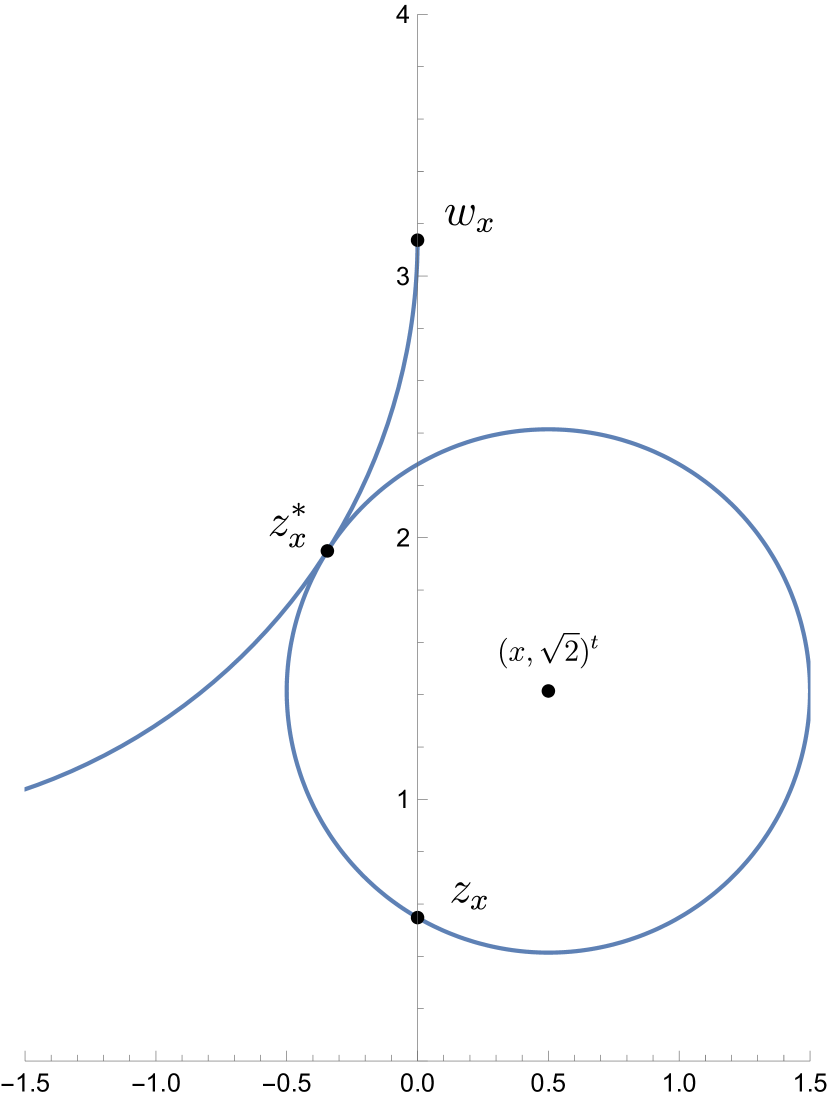
(a) $x=\frac{1}{2}$

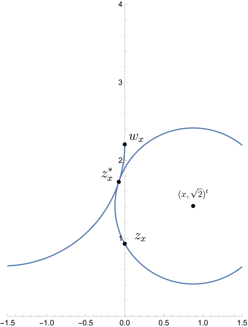
(b) $x=\frac{7}{8}$

Figure 1. Illustration of $C_{x}$ and a section of $\eta_{x}\cdot C^{\prime}$.

Remark 5.22.

It holds that $\operatorname{\mathcal{E}}(\Gamma_{x_{n}})=\operatorname{\mathcal{E}}(\Gamma_{x_{n}}^{\prime})\to 0$ for $n\to\infty$. Firstly, since $\Gamma_{x_{n}}$ and $\Gamma_{x_{n}}^{\prime}$ differ only by an isometry of $\mathbb{H}^{2}$, their elastic energies agree. Further, since $|\vec{\kappa}|_{g}^{2}\equiv 2$ on $\Gamma_{x_{n}}$ by construction, we only need to argue that the hyperbolic length of $\Gamma_{x_{n}}$ converges to $0$ for $n\to\infty$. An immediate geometric consequence of the above construction is that

(5.25) $$|\tau-\langle\tau,(0,1)^{t}\rangle(0,1)^{t}|\leq|\tau_{n}-(0,1)^{t}|$$

for all $\tau\in T_{p}\Gamma_{x_{n}}$ with $|\tau|=1$ and for all $p\in\Gamma_{x_{n}}$ where $\tau_{n}=\gamma_{n}^{\prime}(\frac{K(p_{n})}{r_{n}})/|\gamma_{n}^{\prime}(\frac{K(p_{n})}{r_{n}})|$. That is, the least vertical of all tangent vectors in $\Gamma_{x_{n}}$ is the one at $z_{x_{n}}$. Since $\tau_{n}\to(0,1)^{t}$ and since normalized tangent vectors are invariant under scaling, the claim follows.

We construct the initial datum $u_{0}^{n}$ then as follows. First choose a suitable $W^{2,2}$-parametrization of $\Gamma_{x_{n}}$ starting in $w_{x_{n}}$ and ending in $z_{x_{n}}$. Then, concatenate with a suitable order-reversing reparametrization of $\gamma_{n}|_{[-K(p_{n})/r_{n},K(p_{n})/r_{n}]}$ such that the concatenation is in $W^{2,2}$. Finally, concatenate again with a suitable $W^{2,2}$-parametrization of $\Gamma_{x_{n}}^{\prime}$ starting in $z_{x_{n}}$ and ending in $w_{x_{n}}$ such that the entire curve is in $W^{2,2}$. Now rescale the entire curve we obtained by $1/(w_{x_{n}})^{(2)}$. We denote by $u_{0}^{n}$ the constant $g_{\mathbb{H}^{2}}$-speed reparametrization of the final curve on $[-1,1]$. Compare also Figure 2 for plots of $u_{0}^{n}$ for some values of $\lambda_{n}$. By construction, one obtains

(5.26) $$u_{0}^{n}(\pm 1)=(0,1)^{t}\quad\text{and}\quad(\partial_{s}u_{0}^{n})(\pm 1)=\pm(0,1)^{t}.$$

Note that, by Remarks 5.21 and 5.22, $\operatorname{\mathcal{E}}(u_{0}^{n})\searrow 8$ for $n\to\infty$.

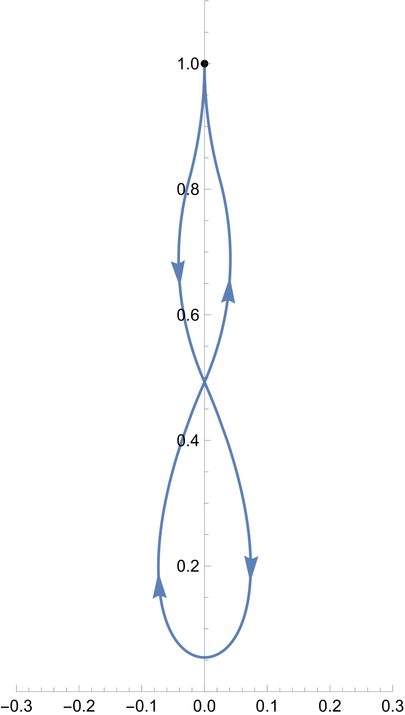
(a) $\lambda_{n}=\frac{2}{5}$

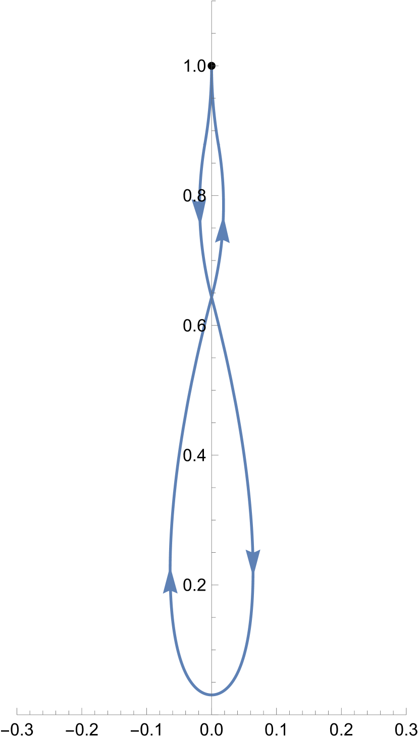
(b) $\lambda_{n}=\frac{1}{10}$

Figure 2. Illustration of the initial datum $u_{0}^{n}$.

Assumption: There is no singularity along the Willmore flow. By short-time existence, there is a maximal solution $u^{n}\colon[0,T_{\mathrm{max},n})\times I\to\mathbb{H}^{2}$ of the Willmore flow (i.e. (3.41) with $a(x,y)=-1/(4y^{4})$) with initial datum $u_{0}^{n}$ as constructed above. The lack of smoothness poses no issue, cf. Remark 3.15. Suppose that $\sup_{t\in[0,T_{\mathrm{max},n})}\mathcal{L}_{\mathbb{H}^{2}}(u^{n})<\infty$. By Theorems 3.14 and 4.5, $T_{\mathrm{max},n}=\infty$ and the constant $g_{\mathbb{H}^{2}}$-speed reparametrizations of $u^{n}$ converge to a critical point $u^{n}_{\infty}$ of $\operatorname{\mathcal{E}}$ parametrized by constant $g_{\mathbb{H}^{2}}$-speed still satisfying the Dirichlet boundary data induced by $u_{0}^{n}$, cf. (5.26). Moreover, $\operatorname{\mathcal{E}}(u^{n}_{\infty})\leq\operatorname{\mathcal{E}}(u_{0}^{n})\to 8$ for $n\to\infty$.

Remark 5.23.

We wish to obtain a contradiction by showing that $u_{\infty}^{n}$ cannot be a critical point of $\operatorname{\mathcal{E}}$ (for $n$ sufficiently large). To this end, we proceed as follows.

1. Argue that $u_{\infty}^{n}$ is necessarily a reparametrization of a simply closed, canonically parametrized free orbit-like elastica.

2. Show that there is no canonically parametrized segment of a free orbit-like elastica satisfying the boundary data in (5.26) to reach a contradiction.

Ad (I). By the boundary data (5.26), $u_{\infty}^{n}$ has a self-intersection. Consequently, as we will argue in Remark 5.25, for $n$ sufficiently large, the only remaining category for $u_{\infty}^{n}$ is that of a free orbit-like elastica.

Since the initial datum $u_{0}^{n}$ satisfies the symmetry relation $u_{0}^{n}(-x)=-\overline{u_{0}^{n}(x)}$ by construction and Lemma 5.15, Lemma 5.17 yields $u^{n}(t,-x)=-\overline{u^{n}(t,x)}$ for any $t\geq 0$ and $x\in[-1,1]$. So by the convergence and Remark 5.18,

(5.27) $$u^{n}_{\infty}(-x)=-\overline{u^{n}_{\infty}(x)}\quad\text{for all $x\in[-1,1]$}.$$

We will show in Lemma 5.28 that, choosing $n$ sufficiently large, this symmetry relation is sufficient for w.l.o.g. supposing that $u_{\infty}^{n}$ is given as a reparametrization of a canonically parametrized orbit-like elastica $\gamma_{\infty}^{n}$. Note that, by (5.27), $u_{\infty}^{n}(0)=iy$ and $\partial_{s}u_{\infty}^{n}(0)=\pm y+0i$ for some $y>0$. Therefore, since $u_{\infty}^{n}$ is parametrized by constant $g_{\mathbb{H}^{2}}$-speed and since $\partial_{s}u_{\infty}^{n}(0)=\pm y+0i$, we have $u_{\infty}^{n}(x)=\gamma_{\infty}^{n}(\pm\ell_{n}\cdot x)$ for $x\in[-1,1]$ where $\ell_{n}>0$ is the smallest positive number with $\gamma^{n}_{\infty}(\ell_{n})=\gamma^{n}_{\infty}(-\ell_{n})$.

Ad (II). Since $\gamma^{n}_{\infty}(\ell_{n})=\gamma^{n}_{\infty}(-\ell_{n})$, Remark 5.16 yields $\gamma^{n}_{\infty}(\ell_{n})=\omega i$ for some $\omega>0$. Moreover, since $\gamma^{n}_{\infty}$ is canonically parametrized, (5.7) and (5.6) yield

(5.28) $$(\gamma_{\infty}^{n})^{\prime}(\ell_{n})=\frac{-a\omega^{2}+c}{\kappa(\ell_{n})^{2}+2i\kappa^{\prime}(\ell_{n})}=\frac{-a\omega^{2}+c}{\kappa(\ell_{n})^{4}+(2\kappa^{\prime}(\ell_{n}))^{2}}(\kappa(\ell_{n})^{2}-2i\kappa^{\prime}(\ell_{n})).$$

Particularly, since $|(\gamma_{\infty}^{n})^{\prime}(\ell_{n})|_{g}=1$, we have $-a\omega^{2}+c\neq 0$. Further, (5.26) yields $\mathrm{Re}((\gamma_{\infty}^{n})^{\prime}(\ell_{n}))=0$ so that (5.28) yields $\kappa(\ell_{n})^{2}=0$. However, by Proposition 5.6, $\kappa^{2}(\ell_{n})=\kappa_{0}^{2}\mathrm{dn}^{2}(r\ell_{n},p)\neq 0$ by Definition A.4. A contradiction!

5.5. Auxiliary results on free elastica

The following closing-condition is a corollary of Theorem 5.10. For notation and some results on the elliptic integrals and functions below, refer to Appendix A. Throughout this section, we use $C$ defined in (5.4) and the notation of Proposition 5.6.

Proposition 5.24.

Consider a free elastica $\gamma\colon I\to\operatorname{\mathbb{R}}$, $\alpha<\beta$ with $\alpha,\beta\in I$ and $\gamma(\alpha)=\gamma(\beta)$. Then $C<0$, i.e., $\gamma$ is either orbit-like or circular. If $\gamma$ is orbit-like and canonically parametrized, it follows that

(5.29) $$\pi\leq m\pi =\frac{1}{2}\sqrt{1-p^{2}}\sqrt{2-p^{2}}\int_{\mathrm{am}(r\alpha,p)}^{\mathrm{am}(r\beta,p)}\frac{\sqrt{1-p^{2}\sin^{2}(\theta)}}{1-p^{2}(2-p^{2})\sin^{2}(\theta)}\,d\theta$$

for some $m\in\operatorname{\mathbb{N}}$. If $\gamma$ is circular, $\operatorname{\mathcal{E}}(\gamma)\geq 4\pi$.

Proof.

Consider the case where $\kappa$ is non-constant. By Lemma 5.8 and Theorem 5.10, there is an isometry $\Phi\colon\mathbb{H}^{2}\to\mathbb{H}^{2}$ such that $\Phi\gamma(s_{*})=i$ and $d\Phi_{\gamma(s_{*})}(\gamma^{\prime}(s_{*}))=1$ for a fixed $s_{*}\in\operatorname{\mathbb{R}}$ with ${\kappa}(s_{*})^{2}=\kappa_{0}^{2}$. Then

(5.30) $$\Phi\gamma(x)=f\left(\int_{s_{*}}^{x}\frac{1}{\theta}\,ds+z_{1}\right)$$

with $f$ as in (5.9) and $\theta$ as in (5.6). Now observe that, by (5.6), (5.4) and Theorem 5.10, $4\kappa^{2}+4C=|\theta|^{2}>0$. Whence,

(5.31) $$\frac{1}{\theta(s)}=\frac{{\kappa}^{2}-2i{\kappa}^{\prime}}{{\kappa}^{4}+4({\kappa}^{\prime})^{2}}\underset{\eqref{eq:char-el-0}}{=}\frac{{\kappa}^{2}}{4C+4{\kappa}^{2}}+i\frac{-2{\kappa}^{\prime}}{4C+4{\kappa}^{2}}.$$

Note that, in either of the last two cases of (5.9), $\gamma(\alpha)=\gamma(\beta)$ yields

(5.32) $$\int_{\alpha}^{\beta}\frac{1}{\theta}\,ds=0.$$

In either of those cases, (5.32) and (5.31) together yield $\kappa\equiv 0$, a contradiction.

Now suppose that $ac<0$. Since $\tanh(z)=\tanh(w)$ if and only if $z-w\in i\pi\operatorname{\mathbb{Z}}$, (5.30), (5.31) and $C=-ac$ yield

(5.33) $$i\pi\operatorname{\mathbb{Z}}\ni\sqrt{C}\int_{\alpha}^{\beta}\frac{1}{\theta}\,ds=\sqrt{C}\int_{\alpha}^{\beta}\frac{\kappa^{2}}{4C+4\kappa^{2}}\,ds+i\sqrt{C}\int_{\alpha}^{\beta}\frac{-2\kappa^{\prime}}{4C+4\kappa^{2}}\,ds.$$

Particularly, we again have $\kappa\equiv 0$, a contradiction.

Whence, only the first two cases in (5.9) remain and $C=-ac<0$, i.e., $\gamma$ is necessarily orbit-like. Moreover, $\tan(z)=\tan(w)$ if and only if $\cot(z)=\cot(w)$ if and only if $z-w\in\pi\operatorname{\mathbb{Z}}$ for $z,w\in\operatorname{\mathbb{C}}$. Therefore, (5.30) and (5.31) yield again

(5.34) $$\pi\operatorname{\mathbb{Z}}\ni\sqrt{-C}\int_{\alpha}^{\beta}\frac{1}{\theta}\,ds=\sqrt{-C}\int_{\alpha}^{\beta}\frac{\kappa^{2}}{4C+4\kappa^{2}}\,ds+i\sqrt{-C}\int_{\alpha}^{\beta}\frac{-2\kappa^{\prime}}{4C+4\kappa^{2}}\,ds.$$

Particularly,

(5.35) $$\int_{\alpha}^{\beta}\frac{-2\kappa^{\prime}}{4C+4\kappa^{2}}\,ds=0\quad\text{and}\quad m\pi=\sqrt{-C}\int_{\alpha}^{\beta}\frac{\kappa^{2}}{4C+4\kappa^{2}}\,ds,$$

for some $m\in\operatorname{\mathbb{N}}$. If $\gamma$ is canonically parametrized, by Proposition 5.6, using

(5.36) $$\kappa^{2}(s)=\kappa_{0}^{2}\mathrm{dn}^{2}(rs,p)=\kappa_{0}^{2}(1-p^{2}\sin^{2}(\mathrm{am}(rs,p))) \partial_{s}\mathrm{am}(s,p)=\mathrm{dn}(s,p)$$ and ,

we have

(5.37) $$\sqrt{-C}\int_{\alpha}^{\beta}\frac{\kappa^{2}}{4C+4\kappa^{2}}\,ds=\frac{\kappa_{0}^{2}\sqrt{-C}}{r}\int_{\mathrm{am}(r\alpha,p)}^{\mathrm{am}(r\beta,p)}\frac{\sqrt{1-p^{2}\sin^{2}(\theta)}}{4C+4\kappa_{0}^{2}(1-p^{2}\sin^{2}(\theta))}\,d\theta.$$

Moreover, Proposition 5.6 yields the following relations:

(5.38) $$\kappa_{0}^{2}=\frac{4}{2-p^{2}},\quad\sqrt{-C}=(\kappa_{0}^{2}-\frac{1}{4}\kappa_{0}^{4})^{\frac{1}{2}}=\frac{2\sqrt{1-p^{2}}}{2-p^{2}},\quad r=\frac{1}{\sqrt{2-p^{2}}}$$

and finally, using (5.4),

(5.39) $$4C+4\kappa_{0}^{2}(1-p^{2}\sin^{2}(\theta)) =\kappa_{0}^{4}-4\kappa_{0}^{2}p^{2}\sin^{2}(\theta)$$

$$=\frac{16}{(2-p^{2})^{2}}\cdot(1-p^{2}(2-p^{2})\sin^{2}(\theta)).$$

Altogether, we conclude (5.29). Now consider the case where $\kappa$ is constant. If $\kappa\equiv 0$, then $\gamma$ has no self-intersections. Otherwise, $\gamma$ is circular and $\operatorname{\mathcal{E}}(\gamma)\geq 4\pi$ by Remark 5.7. ∎

Remark 5.25.

Proposition 5.24 immediately yields the following. If we are considering (segments of) free elastica with self-intersections whose elastic energy is sufficiently close to $8$, only orbit-like elastica need to be taken into account. So we collect further properties of orbit-like elastica in the next lemma.

Lemma 5.26.

For a free canonically parametrized orbit-like elastica $\gamma\colon I\to\mathbb{H}^{2}$, $\gamma(\alpha)=\gamma(\beta)$ for $\alpha<\beta$ already implies that $\mathrm{am}(r\beta,p)-\mathrm{am}(r\alpha,p)>\pi$. If additionally $\alpha^{\prime},\beta^{\prime}\in I$ with $\alpha^{\prime}\leq\alpha<\beta<\beta^{\prime}$ and $\gamma(\alpha^{\prime})=\gamma(\beta^{\prime})$, then $\mathrm{am}(r\beta^{\prime},p)-\mathrm{am}(r\alpha^{\prime},p)>2\pi$.

Proof.

We study the term on the right-hand-side of (5.29). Firstly,

(5.40) $$\frac{1}{2}\sqrt{1-p^{2}} \sqrt{2-p^{2}}\int_{-\frac{\pi}{2}}^{\frac{\pi}{2}}\frac{\sqrt{1-p^{2}\sin^{2}(\theta)}}{1-p^{2}(2-p^{2})\sin^{2}(\theta)}\,d\theta$$

$$=\sqrt{1-p^{2}}\sqrt{2-p^{2}}\int_{0}^{\frac{\pi}{2}}\frac{\sqrt{1-p^{2}\sin^{2}(\theta)}}{1-p^{2}(2-p^{2})\sin^{2}(\theta)}\,d\theta.$$

Moreover, by Definition A.1 and a short computation,

(5.41) $$K(p)+(1-p^{2})\Pi(p^{2}(2-p^{2}),p)=(2-p^{2})\int_{0}^{\frac{\pi}{2}}\frac{\sqrt{1-p^{2}\sin^{2}(\theta)}}{1-p^{2}(2-p^{2})\sin^{2}(\theta)}\,d\theta.$$

Combining (5.40) and (5.41), one thus obtains from (A.4) that

(5.42) $$\frac{1}{2}\sqrt{1-p^{2}} \sqrt{2-p^{2}}\int_{-\frac{\pi}{2}}^{\frac{\pi}{2}}\frac{\sqrt{1-p^{2}\sin^{2}(\theta)}}{1-p^{2}(2-p^{2})\sin^{2}(\theta)}\,d\theta$$

$$<\frac{(1-p^{2})^{\frac{3}{2}}}{\sqrt{2-p^{2}}}\cdot\Big{(}\frac{K(p)}{1-p^{2}}+\frac{\pi}{2}\sqrt{\frac{p^{2}(2-p^{2})}{(1-p^{2}(2-p^{2}))(p^{2}-p^{4})}}\Big{)}$$

for all $p\in(0,1)$. Next, observe that, by (A.2),

(5.43) $$\frac{\sqrt{1-p^{2}}}{\sqrt{2-p^{2}}}K(p)\leq\min\Big{\{}\frac{\pi}{2\sqrt{2-p^{2}}},\sqrt{1-p^{2}}K(p)\Big{\}}.$$

As by (A.5) $\sqrt{1-p^{2}}K(p)\to 0$ for $p\nearrow 1$, (5.43) shows that there is $\eta\in(0,1)$ with

(5.44) $$\frac{\sqrt{1-p^{2}}}{\sqrt{2-p^{2}}}K(p)\leq\eta\cdot\frac{\pi}{2}\quad\text{for all $p\in(0,1)$}.$$

Combining (5.42) and (5.44), we obtain for all $p\in(0,1)$

(5.45) $$\frac{1}{2}\sqrt{1-p^{2}}\sqrt{2-p^{2}}\int_{-\frac{\pi}{2}}^{\frac{\pi}{2}}\frac{\sqrt{1-p^{2}\sin^{2}(\theta)}}{1-p^{2}(2-p^{2})\sin^{2}(\theta)}\,d\theta<(1+\eta)\cdot\frac{\pi}{2}.$$

Since $\sin^{2}$ is $\pi$-periodic and by (5.45), (5.29) cannot be satisfied if $\mathrm{am}(r\beta,p)-\mathrm{am}(r\alpha,p)\leq\pi$.

Now additionally considering $\alpha^{\prime}\leq\alpha<\beta<\beta^{\prime}$ with $\gamma(\alpha^{\prime})=\gamma(\beta^{\prime})$, (5.29) yields

(5.46) $$\pi \leq\frac{1}{2}\sqrt{1-p^{2}}\sqrt{2-p^{2}}\int_{\mathrm{am}(r\alpha,p)}^{\mathrm{am}(r\beta,p)}\frac{\sqrt{1-p^{2}\sin^{2}(\theta)}}{1-p^{2}(2-p^{2})\sin^{2}(\theta)}\,d\theta$$

$$<\frac{1}{2}\sqrt{1-p^{2}}\sqrt{2-p^{2}}\int_{\mathrm{am}(r\alpha^{\prime},p)}^{\mathrm{am}(r\beta^{\prime},p)}\frac{\sqrt{1-p^{2}\sin^{2}(\theta)}}{1-p^{2}(2-p^{2})\sin^{2}(\theta)}\,d\theta=\widetilde{m}\pi$$

for some $\widetilde{m}\in\operatorname{\mathbb{N}}$. Particularly, $\widetilde{m}\geq 2$. Again by (5.45) and the $\pi$-periodicity of $\sin^{2}$, $\mathrm{am}(r\beta^{\prime},p)-\mathrm{am}(r\alpha^{\prime},p)>2\pi$ which shows the remainder of the claim. ∎

Lemma 5.27.

Let $\gamma\colon[\alpha,\beta]\to\mathbb{H}^{2}$ be the canonical parametrization of an orbit-like elastica with parameter $p\in(0,1)$ such that $\mathrm{am}(r\beta,p)-\mathrm{am}(r\alpha,p)>m\pi$ for some $m\in\operatorname{\mathbb{N}}$. Then $\operatorname{\mathcal{E}}(\gamma)>8m$.

Proof.

Using Proposition 5.6, we have $\kappa(s)^{2}=\kappa_{0}^{2}\cdot\mathrm{dn}^{2}(rs,p)\text{ for all $s\in[\alpha,\beta]$}$ where $\kappa_{0}^{2}=\frac{4}{2-p^{2}}$ and $r=\frac{1}{\sqrt{2-p^{2}}}$. Consequently, by the $\pi$-periodicity of $\sin^{2}$,

(5.47) $$\operatorname{\mathcal{E}}(\gamma)=\int_{\alpha}^{\beta}\kappa^{2}(s)\,ds=\sqrt{2-p^{2}}\frac{4}{2-p^{2}}\int_{r\alpha}^{r\beta}\mathrm{dn}^{2}(s,p)\,ds$$

(5.48) $$=\frac{4}{\sqrt{2-p^{2}}}\int_{\mathrm{am}(r\alpha,p)}^{\mathrm{am}(r\beta,p)}\sqrt{1-p^{2}\sin^{2}(\theta)}\,d\theta\geq\frac{8m}{\sqrt{2-p^{2}}}E(p)\underset{\eqref{eq:ieq-Ep}}{>}8m.\qed$$

In the proof of (I) in the previous section, we argue that the limit $u_{\infty}^{n}$ satisfies the same symmetry relation as $u_{0}^{n}$. In order to fully classify the limit with this information, we require the following.

Lemma 5.28.

Let $\gamma\colon[-L,L]\to\mathbb{H}^{2}$ parametrize a free orbit-like elastica with $\gamma(-L)=\gamma(L)$ and with parameter $p\in(0,1)$. Moreover, suppose that

(5.49) $$\gamma(-x)=-\overline{\gamma(x)}\quad\text{for all $x\in[-L,L]$}.$$

Then $\gamma(0)=iy$ and $\gamma^{\prime}(0)=\pm y+0i$ for some $y>0$. Moreover, we either have $\kappa(0)^{2}=\kappa_{0}^{2}(1-p^{2})$ or $\kappa(0)^{2}=\kappa_{0}^{2}$ with $\kappa_{0}^{2}$ as in Proposition 5.6.

Lastly, there exists $\varepsilon>0$ such that, for any $\gamma$ as above with $\kappa(0)^{2}=\kappa_{0}^{2}(1-p^{2})$,

(5.50) $$\operatorname{\mathcal{E}}(\gamma)\geq 8+\varepsilon.$$

Proof.

Indeed, by Remark 5.16 and (5.49), $\kappa^{2}$ needs to be an even function. As $\kappa(s)^{2}=\kappa_{0}^{2}\mathrm{dn}(rs,p)^{2}$ by Proposition 5.6, one concludes that $\kappa(0)^{2}$ either is a local minimum or maximum of $\kappa^{2}$. Thus, using Definition A.4, $\kappa(0)^{2}\in\{\kappa_{0}^{2},\kappa_{0}^{2}(1-p^{2})\}$.

Now suppose that $\kappa(0)^{2}=\kappa_{0}^{2}(1-p^{2})$. Particularly, Proposition 5.6 yields that $\kappa$ is a translation of $s\mapsto\kappa_{0}\cdot\mathrm{dn}(rs,p)$. As $\mathrm{dn}(x,p)=\sqrt{1-p^{2}}$ if and only if $\mathrm{am}(x,p)\in\pi/2+\pi\operatorname{\mathbb{Z}}$ if and only if $x\in K(p)+2K(p)\operatorname{\mathbb{Z}}$ by Definition A.4 and Remark A.5, $\kappa(s)=\kappa_{0}\cdot\mathrm{dn}(rs+K(p),p)$. Moreover, using $m\in\operatorname{\mathbb{N}}$ in (5.35), the assumption $\gamma(-L)=\gamma(L)$ yields that

(5.51) $$\pi\leq\sqrt{-C}\int_{-L}^{L}\frac{\kappa(s)^{2}}{4C+4\kappa(s)^{2}}\,ds.$$

Whence, using (5.38) and (5.39) and Remark A.5,

(5.52) $$\sqrt{-C}\int_{-L}^{L} \frac{\kappa(s)^{2}}{4C+4\kappa(s)^{2}}\,ds=\frac{\sqrt{-C}\kappa_{0}^{2}}{r}\int_{-rL+K(p)}^{rL+K(p)}\frac{\mathrm{dn}(s,p)\partial_{s}\mathrm{am}(s,p)}{4C+4\kappa_{0}^{2}\mathrm{dn}^{2}(s,p)}\,ds$$

$$=8\frac{\sqrt{1-p^{2}}}{(2-p^{2})^{3/2}}\int_{\mathrm{am}(-Lr+K(p),p)}^{\mathrm{am}(Lr+K(p),p)}\frac{\sqrt{1-p^{2}\sin^{2}(\theta)}}{4C+4\kappa_{0}^{2}(1-p^{2}\sin^{2}(\theta))}\,d\theta$$

$$=\frac{1}{2}\sqrt{1-p^{2}}\sqrt{2-p^{2}}\int_{\mathrm{am}(-Lr+K(p),p)}^{\mathrm{am}(Lr+K(p),p)}\frac{\sqrt{1-p^{2}\sin^{2}(\theta)}}{1-p^{2}(2-p^{2})\sin^{2}(\theta)}\,d\theta.$$

Moreover, note that, for $0<\delta<\pi/4$,

(5.53) $$\int_{-\delta}^{0} \frac{\sqrt{1-p^{2}\sin^{2}(\theta)}}{1-p^{2}(2-p^{2})\sin^{2}(\theta)}\,d\theta=\int_{0}^{\delta}\frac{\sqrt{1-p^{2}\sin^{2}(\theta)}}{1-p^{2}(2-p^{2})\sin^{2}(\theta)}\,d\theta$$

$$=\int_{0}^{\delta}\frac{\sqrt{1+(1-p^{2})\tan^{2}(\theta)}\sqrt{1+\tan^{2}(\theta)}}{1+(1-p^{2})^{2}\tan^{2}(\theta)}\,d\theta$$

$$\leq\int_{0}^{\tan(\delta)}\frac{\sqrt{1+(1-p^{2})s^{2}}}{1+(1-p^{2})^{2}s^{2}}\,ds\leq\int_{0}^{\tan(\delta)}\frac{1+(1-p^{2})s^{2}}{1+(1-p^{2})^{2}s^{2}}\,ds\leq 2\tan(\delta)\to 0$$

as $\delta\searrow 0$. Combining the previous estimates and using (5.45), we obtain that there exists $\delta>0$ sufficiently small such that, for all $p\in(0,1)$,

(5.54) $$\frac{1}{2}\sqrt{1-p^{2}}\sqrt{2-p^{2}}\int_{-\delta}^{\pi+\delta}\frac{\sqrt{1-p^{2}\sin^{2}(\theta)}}{1-p^{2}(2-p^{2})\sin^{2}(\theta)}\,d\theta<\pi.$$

Using [5, (122.03)], $(\mathrm{am}(-Lr+K(p),p),\mathrm{am}(Lr+K(p),p))$ is an open interval centered at $\frac{\pi}{2}$. In view of (5.51) and (5.52), by (5.54) and since this interval is the domain of integration on the right-hand-side of (5.52),

(5.55) $$(\mathrm{am}(-Lr+K(p),p),\mathrm{am}(Lr+K(p),p))\supseteq(-\delta,\pi+\delta).$$

Whence, similarly as in (5.47),

(5.56) $$\operatorname{\mathcal{E}}(\gamma) =\frac{4}{\sqrt{2-p^{2}}}\int_{\mathrm{am}(Lr+K(p),p)}^{\mathrm{am}(-Lr+K(p),p)}\sqrt{1-p^{2}\sin^{2}(\theta)}\,d\theta$$

(5.57) $$\geq\frac{4}{\sqrt{2-p^{2}}}\int_{0}^{\pi}\sqrt{1-p^{2}\sin^{2}(\theta)}\,d\theta+\frac{8}{\sqrt{2-p^{2}}}\int_{0}^{\delta}\sqrt{1-p^{2}\sin^{2}(\theta)}\,d\theta$$

(5.58) $$\geq 8+\frac{8}{\sqrt{2}}\int_{0}^{\delta}\sqrt{1-\sin^{2}{\theta}}\,d\theta=\vcentcolon 8+\varepsilon.\qed$$

6. A Li-Yau inequality for open curves in $\mathbb{H}^{2}$

A similar analysis to this section for closed planar curves is undertaken in [27].

Set $W_{\mathrm{imm}}^{2,2}([0,1],\mathbb{H}^{2})\vcentcolon=\{u\in W^{2,2}([0,1],\operatorname{\mathbb{R}}^{2}):u([0,1])\subseteq\mathbb{H}^{2},\text{ $u$ is immersed}\}$, equipped with the Euclidean Sobolev norm.

Theorem 6.1.

Any $u\in W_{\mathrm{imm}}^{2,2}([0,1],\mathbb{H}^{2})$ with $\operatorname{\mathcal{E}}(u)\leq 8$ is an embedding.

Proof.

Define

(6.1) $$\mathcal{A}\vcentcolon=\{\gamma\in W_{\mathrm{imm}}^{2,2}([0,1],\mathbb{H}^{2}):\gamma\text{ non-embedded, }\partial_{s}^{k}\gamma(y)=\partial_{s}^{k}u(y)\text{ for }y,k=0,1\}.$$

We claim that $m\vcentcolon=\inf_{\gamma\in\mathcal{A}}\operatorname{\mathcal{E}}(\gamma)\geq 8$.

To this end, consider a minimizing sequence $(\widetilde{\gamma}_{n})_{n\in\operatorname{\mathbb{N}}}\subseteq\mathcal{A}$ with $\operatorname{\mathcal{E}}(\widetilde{\gamma}_{n})\to m$. Suppose for contradiction that $m<8$. W.l.o.g., $\sup_{n\in\operatorname{\mathbb{N}}}\operatorname{\mathcal{E}}(\widetilde{\gamma}_{n})<8$. Define $\gamma_{n}$ to be the constant $g_{\mathbb{H}^{2}}$-speed reparametrization of $\widetilde{\gamma}_{n}$. Further, using Corollary 2.7, one obtains

(6.2) $$\frac{1}{\gamma_{n}^{(2)}}|\partial_{x}\gamma_{n}|=|\partial_{x}\gamma_{n}|_{g}=\mathcal{L}_{\mathbb{H}^{2}}(\gamma_{n})=\vcentcolon\ell_{n}\leq C$$

for some $C>0$ and for all $n\in\operatorname{\mathbb{N}}$. Further, by Remark 2.8, there are $L,l>0$ such that $l\leq\gamma_{n}^{(2)}\leq L$ uniformly in $n$. Whence, by (6.2), $|\partial_{x}\gamma_{n}|\leq L\ell_{n}$. Moreover, since $\partial_{s_{\gamma_{n}}}=\frac{1}{\ell_{n}}\partial_{x}$ and since, by (2.1) and (2.2),

(6.3) $$\ell_{n}^{2}\vec{\kappa}_{n}=\partial_{x}^{2}\gamma_{n}+\frac{1}{\gamma_{n}^{(2)}}\begin{pmatrix}-2\partial_{x}\gamma_{n}^{(1)}\partial_{x}\gamma_{n}^{(2)}\\ (\partial_{x}\gamma_{n}^{(1)})^{2}-(\partial_{x}\gamma_{n}^{(2)})^{2}\end{pmatrix},$$

we have

(6.4) $$\int_{0}^{1}|\partial_{x}^{2}\gamma_{n}|^{2}\,dx\leq 2\ell_{n}^{4}\int_{0}^{1}|\vec{\kappa}_{n}|^{2}\,dx+{8\ell_{n}^{4}L^{2}}\leq 2\ell_{n}^{4}L^{2}\int_{0}^{1}|\vec{\kappa}_{n}|_{g}^{2}\,ds+{8\ell_{n}^{4}L^{2}}\leq 24C^{4}L^{2}$$

uniformly in $n$. Whence, $(\gamma_{n})_{n\in\operatorname{\mathbb{N}}}\subseteq W^{2,2}$ is uniformly bounded so that, w.l.o.g. passing to a subsequence, $\gamma_{n}\rightharpoonup\gamma$ for some $\gamma\in W^{2,2}$. Since $W^{2,2}([0,1],\operatorname{\mathbb{R}}^{2})\hookrightarrow C^{1}([0,1])$ compactly, we may also suppose that $\gamma_{n}\to\gamma$ in $C^{1}$. As $\gamma_{n}^{(2)}\geq l>0$, $\gamma\colon[0,1]\to\mathbb{H}^{2}$.

By [27, Lemma 4.3 and Remark 4.4], $\gamma$ is non-embedded. As at the beginning of the proof of Theorem 3.14, one deduces from the bound on the elastic energy that the $g_{\mathbb{H}^{2}}$-length $\ell_{n}$ of each $\gamma_{n}$ is bounded from below uniformly away from $0$. Therefore, since $|\partial_{x}\gamma_{n}|_{g}=\ell_{n}$, we obtain $|\partial_{x}\gamma|_{g}>0$. Particularly, $\gamma$ is also immersed and $\gamma\in\mathcal{A}$. Furthermore, it follows that $\operatorname{\mathcal{E}}(\gamma)\leq\liminf_{n\to\infty}\operatorname{\mathcal{E}}(\gamma_{n})=m$. As $\gamma$ is not embedded, there are $0\leq x_{1}<x_{2}\leq 1$ with $\gamma(x_{1})=\gamma(x_{2})$.

Claim:

$\gamma|_{[x_{1},x_{2}]}$ is a reparametrization of a segment of a free elastica.

To this end, consider $\varphi\in C_{c}^{\infty}((x_{1},x_{2}),\operatorname{\mathbb{R}}^{2})$ arbitrary. For $|t|$ sufficiently small, $\gamma+t\varphi\in\mathcal{A}$. By the minimizing property of $\gamma$,

(6.5) $$0=\frac{d}{dt}\Big{|}_{t=0}\operatorname{\mathcal{E}}(\gamma+t\varphi)=\frac{d}{dt}\Big{|}_{t=0}\operatorname{\mathcal{E}}((\gamma+t\varphi)|_{(x_{1},x_{2})}).$$

Now the arguments in [18, Section 5] yield that $\gamma|_{(x_{1},x_{2})}\in C^{\infty}$ solves $\nabla_{L^{2}}\operatorname{\mathcal{E}}(\gamma)=0$ on $(x_{1},x_{2})$. We wish to verify that $\gamma$ remains smooth also on the closure $[x_{1},x_{2}]$. To this end, since $\gamma$ is again parametrized with constant $g_{\mathbb{H}^{2}}$-speed, Lemma 5.9 yields that there is a smooth extension $\widetilde{\gamma}\colon\operatorname{\mathbb{R}}\to\mathbb{H}^{2}$ of $\gamma$. Whence, $\gamma\in C^{\infty}([x_{1},x_{2}])$ and the claim follows.

By Corollary 5.24, Lemma 5.26 and Lemma 5.27, we obtain $\operatorname{\mathcal{E}}(\gamma|_{[x_{1},x_{2}]})>8$; thus contradicting the assumption $\operatorname{\mathcal{E}}(\gamma)<8$. Altogether, we have $m\geq 8$.

This proves that any $u\in W^{2,2}_{\mathrm{imm}}([0,1],\mathbb{H}^{2})$ with $\operatorname{\mathcal{E}}(u)<8$ is necessarily embedded. Now suppose that $\operatorname{\mathcal{E}}(u)=8$ and w.l.o.g. $u(0)=u(1)$. By Remark 3.15, there is a solution $h\colon[0,T)\times[0,1]\to\mathbb{H}^{2}$ of the clamped elastic flow, i.e., (3.41) with $a\equiv-1$, such that $h(0,\cdot)=u$ and $\partial_{x}^{k}h(t,y)=\partial_{x}^{k}u(y)$ for $y,k=0,1$.

Firstly, suppose that $h$ is non-constant. That is, using (2.3) there exists $t^{\prime}>0$ with $\partial_{t}\operatorname{\mathcal{E}}(h(t,\cdot))|_{t=t^{\prime}}<0$. Whence, $\operatorname{\mathcal{E}}(h(t,\cdot))<\operatorname{\mathcal{E}}(h(t^{\prime},\cdot))\leq 8$ for all $t>t^{\prime}$. However $h(t,0)=u(0)=u(1)=h(t,1)$ for such $t$, a contradiction to the above.

Conversely, suppose that $h(t,\cdot)=u$ for all $t\geq 0$. Especially, by Remark 3.15, $u\in C^{\infty}([0,1])$ and, by (3.41), $u$ is a reparametrization of a segment of a free elastica. However, by Corollary 5.24, Lemma 5.26 and Lemma 5.27, there is no non-embedded segment of a free elastica with elastic energy below or equal to $8$. Thus, $\operatorname{\mathcal{E}}(u)>8$, a contradiction. ∎

Remark 6.2.

The energy threshold of $8$ in Theorem 6.1 is optimal in its generality. Indeed, using a sequence $(\gamma_{n})_{n\in\operatorname{\mathbb{N}}}$ of $\lambda_{n}$-figure-eights as in Lemma 5.13 with $\lambda_{n}\searrow 0$, one can consider $\gamma_{n}|_{\left[-{K(p_{n})}/{r_{n}},{K(p_{n})}/{r_{n}}\right]}$, cf. Remark 5.21.

Remark 6.3.

Recall that, by the classical Li-Yau inequality for immersed surfaces in $\operatorname{\mathbb{R}}^{3}$ (cf. [23]) and (1.5), one obtains that any closed, immersed $u\in W^{2,2}(\mathbb{S}^{1},\mathbb{H}^{2})$ with $\operatorname{\mathcal{E}}(u)<16$ is necessarily embedded. Our sufficient energy threshold is lower, but the result allows for a larger class of curves. In fact, the Li-Yau inequality for closed curves can be concluded from our version.

Corollary 6.4.

Let $u_{0}\colon I\to\mathbb{H}^{2}$ be a smooth immersion with $\operatorname{\mathcal{E}}(u_{0})\leq 8$. The solution $u$ to (3.41) exists globally, converges to an embedded critical point of $\operatorname{\mathcal{E}}$ after reparametrization and is embedded for all times $t\geq 0$.

Remark 6.5.

Alternatively, one could try to extend the Li-Yau inequality known for closed surfaces to one for immersed surfaces with boundary and, in the setting of Theorem 6.1, apply it to the surface of revolution $f_{u}$. Following the approach involving Simon’s monotonicity formula (cf. [28, Equation (2.1)]), one obtains for an immersed surface $f\colon\Sigma\to\operatorname{\mathbb{R}}^{3}$ with boundary that

(6.6) $$\mathcal{H}^{0}(f^{-1}(p))\pi\leq\frac{1}{4}\mathcal{W}(f)+\frac{1}{2}\int_{\partial\Sigma}\frac{\nu_{f}\cdot(f-p)}{|f-p|^{2}}\,d\sigma_{f}$$

for $p\in f(\Sigma)$, the outer unit normal $\nu_{f}$ at the boundary and the induced volume element $\sigma_{f}$ on $\partial\Sigma$. One obtains that, if

(6.7) $$\mathcal{W}(f)<8\pi-2\sup_{p\in\operatorname{\mathbb{R}}^{3}}\int_{\partial\Sigma}\frac{\nu_{f}\cdot(f-p)}{|f-p|^{2}}\,d\sigma_{f},$$

then $f$ is necessarily an embedding. Since the integrand converges to $0$ for $|p|\to\infty$, the supremum in the above is either attained or equals $0$. Moreover, as the boundary is at least $C^{2}$, one can argue that the integral is non-singular for any $p\in\operatorname{\mathbb{R}}^{3}$, cf. [28, Equation (4.2)].

Appendix A Elliptic integrals and Jacobi elliptic functions

Definition A.1 (Elliptic integrals).

Let $\alpha,p\in[0,1)$ and $\varphi\in\operatorname{\mathbb{R}}$. Then

1. $\displaystyle K(\varphi,p)\vcentcolon=\int_{0}^{\varphi}\frac{1}{\sqrt{1-p^{2}\sin^{2}(\theta)}}\,d\theta$ is the elliptic integral of first kind,

2. $\displaystyle E(\varphi,p)\vcentcolon=\int_{0}^{\varphi}\sqrt{1-p^{2}\sin^{2}(\theta)}\,d\theta$ the elliptic integral of second kind and

3. $\displaystyle\Pi(\varphi,\alpha^{2},p)\vcentcolon=\int_{0}^{\varphi}\frac{1}{(1-\alpha^{2}\sin^{2}(\theta))\sqrt{1-p^{2}\sin^{2}(\theta)}}\,d\theta$ the elliptic integral of third kind.

In case $\varphi=\frac{\pi}{2}$, one omits $\varphi$ in the above notation and calls the respective terms complete elliptic integrals.

Remark A.2.

As on [22, p.19], one can show that

(A.1) $$E(p)>\sqrt{2-p^{2}}$$

for all $p\in(0,1)$. Moreover, we clearly have

(A.2) $$\sqrt{1-p^{2}}K(p)=\int_{0}^{\frac{\pi}{2}}\frac{\sqrt{1-p^{2}}}{\sqrt{1-p^{2}\sin^{2}(\theta)}}\,d\theta\leq\int_{0}^{\frac{\pi}{2}}1\,d\theta=\frac{\pi}{2}.$$

Lastly, for $0<p^{2}<\alpha^{2}<1$ and $0\leq\varphi<\frac{\pi}{2}$, [5, (117.02)] yields

(A.3) $$\Pi(\alpha^{2},p)+\underbrace{\Pi(p^{2}/\alpha^{2},p)}_{\geq\,K(p)}=K(p)+\frac{\pi}{2}\sqrt{\frac{\alpha^{2}}{(1-\alpha^{2})(\alpha^{2}-p^{2})}}$$

and thus, especially,

(A.4) $$\Pi(\alpha^{2},p)\underset{\eqref{eq:bf-1}}{\leq}\frac{\pi}{2}\sqrt{\frac{\alpha^{2}}{(1-\alpha^{2})(\alpha^{2}-p^{2})}}$$

Lemma A.3.

One has $K(p)=O(\log\left[1/\sqrt{1-p^{2}}\right])$ for $p\nearrow 1$. Particularly,

(A.5) $$\lim_{p\nearrow 1}\sqrt{1-p^{2}}K(p)=0.$$

Proof.

Note that, for $p\nearrow 1$,

(A.6) $$K(p)=\int_{0}^{\frac{\pi}{2}}\frac{1}{\sqrt{1-p^{2}(\sin(\theta))^{2}}}\,d\theta=O(1)+\int_{0}^{\frac{\pi}{4}}\frac{1}{\sqrt{1-p^{2}\cos^{2}(\theta)}}\,d\theta.$$

Using $\sin^{2}+\cos^{2}=1$ and substituting $u=\tan(\theta)$, one obtains

(A.7) $$\int_{0}^{\frac{\pi}{4}} \frac{1}{\sqrt{1-p^{2}\cos^{2}(\theta)}}\,d\theta=\int_{0}^{\frac{\pi}{4}}\frac{\sqrt{1+\tan^{2}(\theta)}}{\sqrt{\tan^{2}(\theta)+1-p^{2}}}\,d\theta=\int_{0}^{1}\frac{1}{\sqrt{u^{2}+1-p^{2}}\sqrt{1+u^{2}}}\,du$$

(A.8) $$\leq\int_{0}^{1}\frac{1}{\sqrt{u^{2}+1-p^{2}}}\,du=\frac{1}{2}\log\big{[}\frac{1+\sqrt{2-p^{2}}}{\sqrt{2-p^{2}}-1}\big{]}\leq\log\big{[}\frac{C}{\sqrt{1-p^{2}}}\big{]}.\qed$$

Definition A.4 (Jacobi elliptic functions).

Let $0<p<1$. We define $\mathrm{am}(\cdot,p)\colon\operatorname{\mathbb{R}}\to\operatorname{\mathbb{R}}$ to be the inverse function of the strictly increasing mapping $\operatorname{\mathbb{R}}\to\operatorname{\mathbb{R}}$, $\varphi\mapsto K(\varphi,p)$. Moreover, one defines $\mathrm{cn}(\cdot,p)\vcentcolon=\cos(\mathrm{am}(\cdot,p))$, $\mathrm{sn}(\cdot,p)\vcentcolon=\sin(\mathrm{am}(\cdot,p))$ and $\mathrm{dn}(\cdot,p)\vcentcolon=\sqrt{1-p^{2}\mathrm{sn}(\cdot,p)}$.

Remark A.5.

We collect some well-known identities. Firstly,

(A.9) $$\partial_{x}\mathrm{cn}(x,p)=-\mathrm{sn}(x,p)\mathrm{dn}(x,p),\qquad \partial_{x}\mathrm{sn}(x,p)=\mathrm{cn}(x,p)\mathrm{dn}(x,p)$$

(A.10) $$\partial_{x}\mathrm{dn}(x,p)=-p^{2}\mathrm{cn}(x,p)\mathrm{sn}(x,p), \partial_{x}\mathrm{am}(x,p)=\mathrm{dn}(x,p).$$

All periods of the elliptic functions are given as follows where $l\in\operatorname{\mathbb{Z}}$ and $x\in\operatorname{\mathbb{R}}$.

(A.11) $$\mathrm{am}(lK(p),p)=l\frac{\pi}{2},\qquad \mathrm{cn}(x+4lK(p),p)=\mathrm{cn}(x,p),$$

(A.12) $$\mathrm{sn}(x+4lK(p),p)=\mathrm{sn}(x,p), \mathrm{dn}(x+2lK(p),p)=\mathrm{dn}(x,p).$$

Appendix B Proof of Lemma 5.19

Proof of Lemma 5.19..

For contradiction, after passing to a subsequence, suppose that there exists $M>0$ with

(B.1) $$\frac{1-p_{n}^{2}}{\lambda_{n}^{2}}\leq M\quad\text{for all $n\in\operatorname{\mathbb{N}}$}.$$

By [26, (6.1)], the parameters $p_{n}$ and $\lambda_{n}$ must satisfy

(B.2) $$0 =\int_{0}^{\frac{\pi}{2}}\frac{\sin^{2}(\theta)-\frac{\lambda_{n}}{\kappa_{0}^{2}}}{\left(1-\frac{4\kappa_{0}^{2}}{(\kappa_{0}^{2}-\lambda_{n})^{2}}\cos^{2}(\theta)\right)\sqrt{1-p_{n}^{2}\cos^{2}(\theta)}}\,d\theta\quad\text{for all $n\in\operatorname{\mathbb{N}}$}$$

where

(B.3) $$\kappa_{0}^{2}=\frac{(2\lambda_{n}+4)p_{n}^{2}}{2p_{n}^{2}-1}.$$

One can compute that $p_{n}^{2}-\frac{4\kappa_{0}^{2}}{(\kappa_{0}^{2}-\lambda_{n})^{2}}=\frac{p_{n}^{2}(4+\lambda_{n}-4p_{n}^{2})^{2}}{(\lambda_{n}+4p_{n}^{2})^{2}}>0$. Especially, $\frac{4\kappa_{0}^{2}}{(\kappa_{0}^{2}-\lambda_{n})^{2}}<1$ and (B.2) is well-defined. Firstly, $\int_{\frac{\pi}{4}}^{\frac{\pi}{2}}\frac{\sin^{2}(\theta)-{\lambda_{n}}/{\kappa_{0}^{2}}}{\left(1-{4\kappa_{0}^{2}}/{(\kappa_{0}^{2}-\lambda_{n})^{2}}\cos^{2}(\theta)\right)\sqrt{1-p_{n}^{2}\cos^{2}(\theta)}}\,d\theta$ is non-singular for $n\to\infty$. So we only consider the integral on $[0,\pi/4]$. Next,

(B.4) $$\int_{0}^{\frac{\pi}{4}} \frac{\sin^{2}(\theta)}{\big{(}1-\frac{4\kappa_{0}^{2}}{(\kappa_{0}^{2}-\lambda_{n})^{2}}\cos^{2}(\theta)\big{)}\sqrt{1-p_{n}^{2}\cos^{2}(\theta)}}\,d\theta$$

$$=\int_{0}^{\frac{\pi}{4}}\frac{\tan^{2}(\theta)\sqrt{1+\tan^{2}(\theta)}}{\big{(}\tan^{2}(\theta)+1-\frac{4\kappa_{0}^{2}}{(\kappa_{0}^{2}-\lambda_{n})^{2}}\big{)}\sqrt{\tan^{2}(\theta)+1-p_{n}^{2}}}\,d\theta$$

$$=\int_{0}^{1}\frac{\vartheta^{2}}{\big{(}\vartheta^{2}+1-\frac{4\kappa_{0}^{2}}{(\kappa_{0}^{2}-\lambda_{n})^{2}}\big{)}\sqrt{\vartheta^{2}+1-p_{n}^{2}}\sqrt{1+\vartheta^{2}}}\,d\vartheta.$$

Let $\varepsilon\in(0,1)$ and consider again the integral

(B.5) $$\int_{0}^{1} \frac{\vartheta^{2}}{\big{(}\vartheta^{2}+\underbrace{1-\frac{4\kappa_{0}^{2}}{(\kappa_{0}^{2}-\lambda_{n})^{2}}}_{=\vcentcolon A_{n}}\big{)}\sqrt{\vartheta^{2}+\smash[b]{\underbrace{1-p_{n}^{2}}_{=\vcentcolon B_{n}}}}\sqrt{1+\vartheta^{2}}}\,d\vartheta$$

$$\leq\varepsilon\int_{0}^{\varepsilon}\frac{\theta}{(\theta^{2}+A_{n})\sqrt{\theta^{2}+B_{n}}}\,d\theta+\int_{\varepsilon}^{1}\frac{\theta}{(\theta^{2}+A_{n})\sqrt{\theta^{2}+B_{n}}}\,d\theta$$

$$=\varepsilon\frac{\arctan\big{(}\sqrt{\frac{B_{n}+\varepsilon^{2}}{A_{n}-B_{n}}}\big{)}-\arcsin\big{(}\sqrt{\frac{B_{n}}{A_{n}}}\big{)}}{\sqrt{A_{n}-B_{n}}}+\frac{\arcsin\big{(}\sqrt{\frac{1+B_{n}}{1+A_{n}}}\big{)}-\arctan\big{(}\sqrt{\frac{B_{n}+\varepsilon^{2}}{A_{n}-B_{n}}}\big{)}}{\sqrt{A_{n}-B_{n}}}$$

$$\leq\frac{\varepsilon\pi}{2}\frac{1}{\sqrt{A_{n}-B_{n}}}+\frac{\arcsin\big{(}\sqrt{\frac{1+B_{n}}{1+A_{n}}}\big{)}-\arctan\big{(}\sqrt{\frac{B_{n}+\varepsilon^{2}}{A_{n}-B_{n}}}\big{)}}{\sqrt{A_{n}-B_{n}}}.$$

Now note that, for $n$ sufficiently large, $p_{n}\geq\frac{1}{2}$ and $\lambda_{n}\leq 1$ so that, using (B.1),

(B.6) $$\sqrt{A_{n}-B_{n}}=\frac{p_{n}(4(1-p_{n}^{2})+\lambda_{n})}{\lambda+4p_{n}^{2}}\;\smash{\begin{cases}\geq\frac{1}{10}\lambda_{n}\text{ and}\\ \leq 4\frac{1-p_{n}^{2}}{\lambda_{n}^{2}}\lambda_{n}^{2}+\lambda_{n}\leq(1+4M)\lambda_{n}.\end{cases}}$$

Moreover, $\sqrt{\frac{1+B_{n}}{1+A_{n}}}\nearrow 1$ and, by (B.6),

(B.7) $$\frac{\sqrt{B_{n}+\varepsilon^{2}}}{\sqrt{A_{n}-B_{n}}}\geq\frac{\varepsilon}{\sqrt{(1+4M)\lambda_{n}}}\to\infty.$$

Whence,

(B.8) $$\arcsin\frac{\sqrt{1+B_{n}}}{\sqrt{1+A_{n}}}-\arctan\frac{\sqrt{B_{n}+\varepsilon^{2}}}{\sqrt{A_{n}-B_{n}}}\to\frac{\pi}{2}-\frac{\pi}{2}=0.$$

Particularly, we conclude for (B.5) that

(B.9) $$\int_{0}^{1} \frac{\vartheta^{2}}{\big{(}\vartheta^{2}+1-\frac{4\kappa_{0}^{2}}{(\kappa_{0}^{2}-\lambda_{n})^{2}}\big{)}\sqrt{\vartheta^{2}+1-p_{n}^{2}}\sqrt{1+\vartheta^{2}}}\,d\vartheta\leq\frac{5\pi\varepsilon+o(1)}{\lambda_{n}}.$$

For the second contribution in (B.2), using that $A_{n}\geq B_{n}$,

(B.10) $$\int_{0}^{\frac{\pi}{4}} \frac{-\frac{\lambda_{n}}{\kappa_{0}^{2}}}{\big{(}1-\frac{4\kappa_{0}^{2}}{(\kappa_{0}^{2}-\lambda_{n})^{2}}\cos^{2}(\theta)\big{)}\sqrt{1-p_{n}^{2}\cos^{2}(\theta)}}\,d\theta$$

$$=-\frac{\lambda_{n}}{\kappa_{0}^{2}}\int_{0}^{\frac{\pi}{4}}\frac{(1+\tan^{2}(\theta))^{\frac{3}{2}}}{\big{(}\tan^{2}(\theta)+1-\frac{4\kappa_{0}^{2}}{(\kappa_{0}^{2}-\lambda_{n})^{2}}\big{)}\sqrt{\tan^{2}(\theta)+1-p_{n}^{2}}}\,d\theta$$

$$=-\frac{\lambda_{n}}{\kappa_{0}^{2}}\int_{0}^{1}\frac{\sqrt{1+\vartheta^{2}}}{\big{(}\vartheta^{2}+1-\frac{4\kappa_{0}^{2}}{(\kappa_{0}^{2}-\lambda_{n})^{2}}\big{)}\sqrt{\vartheta^{2}+1-p_{n}^{2}}}\,d\vartheta$$

$$\leq-\frac{\lambda_{n}}{\kappa_{0}^{2}}\int_{0}^{1}\frac{1}{\big{(}\vartheta^{2}+1-\frac{4\kappa_{0}^{2}}{(\kappa_{0}^{2}-\lambda_{n})^{2}}\big{)}^{\frac{3}{2}}}\,d\vartheta.$$

This integral can be explicitly computed (using $\int_{0}^{1}1/(\vartheta^{2}+\Lambda)^{3/2}\,d\vartheta=\frac{1}{\Lambda\sqrt{1+\Lambda}}$ for $\Lambda>0$). Also using (B.3) to evaluate $\kappa_{0}^{2}$, one arrives at

(B.11) $$\int_{0}^{\frac{\pi}{4}} \frac{-\frac{\lambda_{n}}{\kappa_{0}^{2}}}{\big{(}1-\frac{4\kappa_{0}^{2}}{(\kappa_{0}^{2}-\lambda_{n})^{2}}\cos^{2}(\theta)\big{)}\sqrt{1-p_{n}^{2}\cos^{2}(\theta)}}\,d\theta$$

$$\leq-\frac{\lambda_{n}}{\kappa_{0}^{2}}\frac{(\lambda_{n}+4p_{n}^{2})^{3}}{\sqrt{2}\sqrt{\lambda_{n}^{2}+8p_{n}^{2}+12\lambda_{n}p_{n}^{2}-8\lambda_{n}p_{n}^{4}}(\lambda_{n}^{2}+16p_{n}^{2}(1-p_{n}^{2})+16\lambda_{n}p_{n}^{2}(1-p_{n}^{2}))}$$

$$\leq-\frac{1}{\sqrt{42}\kappa_{0}^{2}}\frac{(\lambda_{n}+4p_{n}^{2})^{3}}{\lambda_{n}+16\frac{1-p_{n}^{2}}{\lambda_{n}}+16(1-p_{n}^{2})}=-\frac{1}{\lambda_{n}}\cdot\frac{1}{\sqrt{42}\kappa_{0}^{2}}\frac{(\lambda_{n}+4p_{n}^{2})^{3}}{1+16\frac{1-p_{n}^{2}}{\lambda_{n}^{2}}+16\lambda_{n}\frac{1-p_{n}^{2}}{\lambda_{n}^{2}}}$$

$$\underset{\eqref{eq:lf8-vh-1.1}}{\leq}-\frac{C(M)}{\lambda_{n}}.$$

Altogether, we have that

(B.12) $$\int_{0}^{\frac{\pi}{4}} \frac{\cos^{2}(\theta)-\frac{\lambda_{n}}{\kappa_{0}^{2}}}{\big{(}1-\frac{4\kappa_{0}^{2}}{(\kappa_{0}^{2}-\lambda_{n})^{2}}\sin^{2}(\theta)\big{)}\sqrt{1-p_{n}^{2}\sin^{2}(\theta)}}\,d\theta$$

$$\leq\frac{5\pi\varepsilon+o(1)-C(M)}{\lambda_{n}}\to-\infty\quad\text{as $n\to\infty$,}$$

if we choose $\varepsilon$ sufficiently small. Thus, we obtain a contradiction to (B.2)! ∎

References

- [1] J. W. Barrett, H. Garcke, and R. Nürnberg. Stable approximations for axisymmetric Willmore flow for closed and open surfaces. ESAIM. Mathematical Modelling and Numerical Analysis, 55(3):833–885, 2021.
- [2] M. Bergner, A. Dall’Acqua, and S. Fröhlich. Symmetric Willmore surfaces of revolution satisfying natural boundary conditions. Calculus of Variations and Partial Differential Equations, 39(3-4):361–378, 2010.
- [3] S. Blatt. A singular example for the Willmore flow. Analysis. International Mathematical Journal of Analysis and its Applications, 29(4):407–430, 2009.
- [4] R. Bryant and P. Griffiths. Reduction for constrained variational problems and . American Journal of Mathematics, 108(3):525–570, 1986.
- [5] P. F. Byrd and M. D. Friedman. Handbook of elliptic integrals for engineers and physicists. Die Grundlehren der mathematischen Wissenschaften in Einzeldarstellungen mit besonderer Berücksichtigung der Anwendungsgebiete. Band LXVII. Springer-Verlag, Berlin-Göttingen-Heidelberg, 1954.
- [6] R. Chill. On the Łojasiewicz-Simon gradient inequality. Journal of Functional Analysis, 201(2):572–601, 2003.
- [7] A. Dall’Acqua, K. Deckelnick, and H.-C. Grunau. Classical solutions to the Dirichlet problem for Willmore surfaces of revolution. Advances in Calculus of Variations, 1(4):379–397, 2008.
- [8] A. Dall’Acqua, K. Deckelnick, and G. Wheeler. Unstable Willmore surfaces of revolution subject to natural boundary conditions. Calculus of Variations and Partial Differential Equations, 48(3-4):293–313, 2013.
- [9] A. Dall’Acqua, S. Fröhlich, H.-C. Grunau, and F. Schieweck. Symmetric Willmore surfaces of revolution satisfying arbitrary Dirichlet boundary data. Advances in Calculus of Variations, 4(1):1–81, 2011.
- [10] A. Dall’Acqua, M. Müller, R. M. Schätzle, and A. Spener. The Willmore flow of tori of revolution. arXiv:2005.13500, 2020.
- [11] A. Dall’Acqua and P. Pozzi. A Willmore-Helfrich -flow of curves with natural boundary conditions. Communications in Analysis and Geometry, 22(4):617–669, 2014.
- [12] A. Dall’Acqua, P. Pozzi, and A. Spener. The Łojasiewicz-Simon gradient inequality for open elastic curves. Journal of Differential Equations, 261(3):2168–2209, 2016.
- [13] A. Dall’Acqua and A. Spener. The elastic flow of curves in the hyperbolic plane. arXiv:1710.09600, 2017.
- [14] A. Dall’Acqua and A. Spener. Circular solutions to the elastic flow in hyperbolic space. Proceedings of the conference Analysis on Shapes of Solutions to Partial Differential Equations, 2082:109–124, 2018.
- [15] K. Deckelnick and H.-C. Grunau. Boundary value problems for the one-dimensional Willmore equation. Calculus of Variations and Partial Differential Equations, 30(3):293–314, 2007.
- [16] K. Deckelnick and H.-C. Grunau. A Navier boundary value problem for Willmore surfaces of revolution. Analysis. International Mathematical Journal of Analysis and its Applications, 29(3):229–258, 2009.
- [17] G. Dziuk, E. Kuwert, and R. Schätzle. Evolution of elastic curves in : existence and computation. SIAM Journal on Mathematical Analysis, 33(5):1228–1245, 2002.
- [18] S. Eichmann and H.-C. Grunau. Existence for Willmore surfaces of revolution satisfying non-symmetric Dirichlet boundary conditions. Advances in Calculus of Variations, 12(4):333–361, 2019.
- [19] E. Kuwert and R. Schätzle. The Willmore flow with small initial energy. Journal of Differential Geometry, 57(3):409–441, 2001.
- [20] E. Kuwert and R. Schätzle. Gradient flow for the Willmore functional. Communications in Analysis and Geometry, 10(2):307–339, 2002.
- [21] E. Kuwert and R. Schätzle. Removability of point singularities of Willmore surfaces. Annals of Mathematics. Second Series, 160(1):315–357, 2004.
- [22] J. Langer and D. A. Singer. The total squared curvature of closed curves. J. Differential Geom., 20(1):1–22, 1984.
- [23] P. Li and S. T. Yau. A new conformal invariant and its applications to the Willmore conjecture and the first eigenvalue of compact surfaces. Inventiones Mathematicae, 69(2):269–291, 1982.
- [24] U. F. Mayer and G. Simonett. A numerical scheme for axisymmetric solutions of curvature-driven free boundary problems, with applications to the Willmore flow. Interfaces and Free Boundaries. Modelling, Analysis and Computation, 4(1):89–109, 2002.
- [25] J.-H. Metsch. On the area-preserving Willmore flow of small bubbles sliding on a domain’s boundary. arXiv:2203.12956, 2022.
- [26] M. Müller and A. Spener. On the convergence of the elastic flow in the hyperbolic plane. Geometric Flows, 5(1):40–77, 2020.
- [27] M. Müller and F. Rupp. A Li–Yau inequality for the 1-dimensional Willmore energy. Advances in Calculus of Variations, page 000010151520210014, 2021.
- [28] M. Novaga and M. Pozzetta. Connected surfaces with boundary minimizing the Willmore energy. Mathematics in Engineering, 2(3):527–556, 2020.
- [29] M. Pozzetta. Convergence of elastic flows of curves into manifolds. Nonlinear Analysis. Theory, Methods & Applications. An International Multidisciplinary Journal, 214:Paper No. 112581, 53, 2022.
- [30] F. Rupp and A. Spener. Existence and convergence of the length-preserving elastic flow of clamped curves. arXiv:2009.06991, 2020.
- [31] R. Schätzle. The Willmore boundary problem. Calculus of Variations and Partial Differential Equations, 37(3-4):275–302, 2010.