Data-dependent Generalization Bounds
via Variable-Size Compressibility

Abstract

In this paper, we establish novel data-dependent upper bounds on the generalization error through the lens of a “variable-size compressibility” framework that we introduce newly here. In this framework, the generalization error of an algorithm is linked to a variable-size ‘compression rate’ of its input data. This is shown to yield bounds that depend on the empirical measure of the given input data at hand, rather than its unknown distribution. Our new generalization bounds that we establish are tail bounds, tail bounds on the expectation, and in-expectations bounds. Moreover, it is shown that our framework also allows to derive general bounds on any function of the input data and output hypothesis random variables. In particular, these general bounds are shown to subsume and possibly improve over several existing PAC-Bayes and data-dependent intrinsic dimension-based bounds that are recovered as special cases, thus unveiling a unifying character of our approach. For instance, a new data-dependent intrinsic dimension-based bound is established, which connects the generalization error to the optimization trajectories and reveals various interesting connections with the rate-distortion dimension of a process, the Rényi information dimension of a process, and the metric mean dimension.

I Introduction and problem setup

Let $Z\in\mathcal{Z}$ be some input data distributed according to an unknown distribution $\mu$, where $\mathcal{Z}$ is the data space. A major problem in statistical learning is to find a hypothesis (model) $w$ in the hypothesis space $\mathcal{W}$ that minimizes the population risk defined as [1]

$$\mathcal{L}(w)\coloneqq\mathbb{E}_{Z\sim\mu}\left[\ell(Z,w)\right],\quad w\in\mathcal{W},$$ (1)

where $\ell:\mathcal{Z}\times\mathcal{W}\to\mathbb{R}^{+}$ is a loss function that measures the quality of the prediction of the hypothesis $w\in\mathcal{W}$. The distribution $\mu$ is assumed to be unknown, however; and one has only access to $n$ (training) samples $S=\{Z_{1},\ldots,Z_{n}\}\sim P_{S}=\mu^{\otimes n}$ of the input data. Let $\mathcal{A}\colon\mathcal{S}\rightarrow\mathcal{W}$, $\mathcal{S}=\mathcal{Z}^{n}$, be a possibly stochastic algorithm which, for a given input data $s=\{z_{1},\ldots,z_{n}\}\in\mathcal{Z}^{n}$, picks the hypothesis $\mathcal{A}(s)=W\in\mathcal{W}$. This induces a conditional distribution $P_{W|S}$ on the hypothesis space $\mathcal{W}$. Instead of the population risk minimization problem (1) one can consider minimizing the empirical risk, given by

$$\mathcal{\hat{L}}(s,w)\coloneqq\frac{1}{n}\sum\nolimits_{i=1}^{m}\ell(z_{i},w).$$ (2)

Nonetheless, the minimization of the empirical risk (or a regularized version of it) is meaningful only if the difference between the population and empirical risks is small enough. This difference is known as the generalization error of the learning algorithm and is given by

$$\operatorname{gen}(s,\mathcal{A}(s))\coloneqq\mathcal{L}(\mathcal{A}(s))-\mathcal{\hat{L}}(s,\mathcal{A}(s)).$$ (3)

An exact analysis of the statistical properties of the generalization error (3) is out-of-reach, however, except in very few special cases; and, often, one resorts to bounding the generalization error from the above, instead. The last two decades have witnessed the development of various such upper bounds, from different perspectives and by undertaking approaches that often appear unrelated. Common approaches include information-theoretic, compression-based, fractal-based, or intrinsic-dimension-based, and PAC-Bayes ones. Initiated by Russo and Zou [2]and Xu and Raginsky [3], the information-theoretic approach measures the complexity of the hypothesis space by the Shannon mutual information between the input data and the algorithm output. See also the follow up works [4, 5, 6, 7, 8, 9, 10, 11, 12]. The roots of compression-based approaches perhaps date back to Littlestone and Warmuth [13] who studied the predictability of the training data labels using only part of the dataset. This compressibility approach has been extended in various ways in several subsequent works, including to elaborate data-dependent bounds such as in [14, 15, 16, 17, 18] and [19]. Closer to our work is another popular compressibility approach that studies the compressibility of the hypothesis space, see, e.g., [20, 21, 22, 23] and the recent [24]. The fractal-based approach is a recently initiated line of work that hinges on that when the algorithm has a recursive nature, e.g., it involves an iterative optimization procedure, it might generate a fractal structure either in the model trajectories [25, 26, 27, 28] or in its distribution [29]. These works show that, in that case, the generalization error is controlled by the intrinsic dimension of the generated fractal structure. The original PAC-Bayes bounds were stated for classification [30, 31]; and, it has then become clear that the results could be extended to any bounded loss, resulting in many variants and extensions of them [32, 33, 34, 35, 36, 37, 38, 39, 40, 41, 42, 43, 44, 45]. For more details on PAC-Bayes bounds, we refer the reader to Cantoni’s book [46] or the tutorial paper of [47].

The aforementioned approaches have evolved independently of each other; and the bounds obtained with them differ in many ways that it is generally difficult to compare them. Arguably, however, the most useful bounds must be computable. This means that the bound should depend on the particular sample of the input data at hand, rather than just on the distribution of the data which is unknown. Such bounds are called data-dependent; they are preferred and are generally of bigger utility in practice. In this sense, most existing information-theoretic and rate-distortion theoretic-based bounds on the generalization error are data-independent. This includes the mutual information bounds of Russo and Zou [2] and Xu and Raginsky [3] whose computation requires knowledge of the joint distribution of the input data and output hypothesis; and, as such, they are not computable with just one sample training dataset at hand. In fact, the most prominent data-dependent bounds are those obtained with the PAC-Bayes approach. Note that although their numerical evaluation may not be straightforward in general, especially for large neural networks, a few works have leveraged the compressibility/pruning principle to compute the PAC-Bayes bounds [49, 50].

Contributions. In this paper, we establish novel data-dependent generalization bounds through the lens of a “variable-size compressibility” framework that we introduce here. In this framework, the generalization error of an algorithm is linked to a variable-size ‘compression rate’ of the input data. This allows us to derive bounds that depend on the particular empirical measure of the input data, rather than its unknown distribution. The novel generalization bounds that we establish are tail bounds, tail bounds on the expectation, and in-expectations bounds. Moreover, we show that our variable-size compressibility approach is somewhat generic and it can be used to derive general bounds on any function of the input data and output hypothesis random variables – In particular, see our general tail bound of Theorem 3 in Section III-A as well as other bounds in that section. In fact, as we show, the framework can be accommodated easily to encompass various forms of tail bounds, tail bounds on the expectation, and in-expectation bounds through judicious choices of the distortion measure. In particular, in Section IV, by specializing them we show that our general variable-size compressibility bounds subsume various existing data-dependent PAC-Bayes and intrinsic-dimension-based bounds and recover them as special cases. Hence, another advantage of our approach is that it builds a unifying framework that allows formal connections with the aforementioned, seemingly unrelated, Rate-distortion theoretic, PAC-Bayes, and dimension-based approaches.

In some cases, our bounds are shown to be novel and possibly tighter than the existing ones. For example, see Proposition 1 for an example new data-dependent PAC-Bayes type bound that we obtain readily by application of our general bounds and some judicious choices of the involved variables. Also, our Theorem 7 provides a new dimension-based type bound, which states that the average generalization error over the trajectories of a given algorithm can be upper bounded in terms of the amount of compressibility of such optimization trajectories, measured in terms of a suitable rate-distortion function. This unveils novel connections between the generalization error and newly considered data-dependent intrinsic dimensions, including the rate-distortion dimension of a process, the metric mean dimension, and the Rényi information dimension of a process. The latter is sometimes used in the related literature to characterize the fundamental limits of compressed sensing algorithms. We emphasize that the key ingredient to our approach is the new “variable-size compressibility” framework that we introduce here. For instance, the framework of [24], which comparatively can be thought of as being of “fixed-size” compressibility type, only allows to derive data-independent bounds; and, so, it falls shorts of establishing any meaningful connections with PAC-Bayes and data-dependent intrinsic dimension-based bounds. This is also reflected in the proof techniques in our case which are different from those for the fixed-size compressibility framework.

The rest of this paper is organized as follows. In Section II, we introduce our variable-size compressibility framework and provide a data-dependent tail bound on the generalization error. Section III contains our general bounds. Section IV provides various applications of our main results, in particular, to establish PAC-Bayes and dimension-based bounds. The proofs, as well as other related results, are deferred to the appendices.

Notations.

We denote random variables, their realizations, and their alphabets by upper-case letters, lower-case letters, and calligraphy fonts; e.g., $X$, $x$, and $\mathcal{X}$. The distribution, the expected value, and the support set of a random variable $X$ are denoted as $P_{X}$, $\mathbb{E}[X]$, and $\operatorname{supp}(P_{X})$. A random variable $X$ is called $\sigma$-subgaussian, if $\log\mathbb{E}[\exp(\lambda(X-\mathbb{E}[X]))]\leq\lambda^{2}\sigma^{2}/2$, $\forall\lambda\in\mathbb{R}$. A collection of $m\in\mathbb{N}$ random variables $(X_{1},\ldots,X_{m})$ is denoted as $X^{m}$ or $\mathbf{X}$, when $m$ is known by the context. The notation $\{x_{i}\}_{i=1}^{m}$ is used to represent $m$ real numbers; used also similarly for sets or functions. We use the shorthand notation $[m]$ to denote integer ranges from $1$ to $m\in\mathbb{N}$. Finally, the non-negative real numbers are denoted by $\mathbb{R}^{+}$.

Most of our results are expressed in terms of information-theoretic functions. For two distributions $P$ and $Q$ defined on the same measurable space, define the Rényi divergence of order $\alpha\in\mathbb{R}$, when $\alpha\neq 1$, as $D_{\alpha}\left(Q\|P\right)\coloneqq\frac{1}{\alpha-1}\log\mathbb{E}_{Q}\left[\left(\frac{\mathrm{d}Q}{\mathrm{d}P}\right)^{\alpha-1}\right]$, if $Q\ll P$, and $\infty$ otherwise. Here, $\frac{\mathrm{d}Q}{\mathrm{d}P}$ is the Radon-Nikodym derivative of $Q$ with respect to $P$. The Kullback–Leibler (KL) divergence is defined as $D_{KL}\left(Q\|P\right)\coloneqq\mathbb{E}_{Q}\left[\log\frac{\mathrm{d}Q}{\mathrm{d}P}\right]$, if $Q\ll P$, and $\infty$ otherwise. Note that $\lim_{\alpha\to 1}D_{\alpha}(Q\|P)=D_{KL}(Q\|P)$. The mutual information between two random variables $X$ and $Y$, distributed jointly according to $P_{X,Y}$ with marginal $P_{X}$ and $P_{Y}$, is defined as $I(X;Y)\coloneqq D_{KL}\left(P_{X,Y}\|P_{X}P_{Y}\right)$. This quantity somehow measures the amount of information $X$ has about $Y$, and vice versa. Finally, throughout we will make extensive usage of the following sets, defined for a random variable $X\in\mathcal{X}$ with distribution $P_{X}$ and a real-valued function $g(X)\colon\mathcal{X}\to\mathbb{R}$ as

$$\mathcal{G}_{X}^{\delta}\coloneqq \left\{\nu_{X}\in\mathcal{P}_{\mathcal{X}}\colon D_{KL}\left(\nu_{X}\|P_{X}\right)\leq\log(1/\delta)\right\},$$ (4)

$$\mathcal{S}_{X}\left(g(X)\right)\coloneqq \left\{\nu_{X}\in\mathcal{P}_{\mathcal{X}}\,\big{|}\,\forall x\in\operatorname{supp}(\nu_{X})\colon g(x)>0\right\},$$ (5)

where $\mathcal{P}_{\mathcal{X}}$ is the set of all distributions defined over $\mathcal{X}$.

II Variable-size compressibility

As we already mentioned, the approach of Sefidgaran et al. [24] is based on a fixed-size compressibility framework; and, for this reason, it only accommodates bounds on the generalization error that are independent of the data. In this work, we develop a “variable-size” compressibility framework, which is more general and allows us to establish new data-dependent bounds on the generalization error. As it will become clearer throughout, in particular, this allows us to build formal connections with seemingly-unrelated approaches such as PAC-Bayes and data-dependent intrinsic dimension bounds.

We start by recalling the aforementioned fixed-size compressibility framework, which itself can be seen as an extension of the classic compressibility framework found in source coding literature. We refer the reader to [51] for an easy introduction to classic rate-distortion theory. It should be noted that the rate-distortion theory was also used in [55] to study how the generalization error of the “compressed model” deviates from that of the original (uncompressed) model. Here, similar to [24], we use the rate-distortion theory to bound the generalization error of the original model.

Consider a learning algorithm $\mathcal{A}(S)\colon\mathcal{S}\to\mathcal{W}$. The goal of the compression for the generalization error problem is to find a suitable compressed learning algorithm $\mathcal{\hat{A}}(S,W)=\hat{W}\in\mathcal{\hat{W}}\subseteq\mathcal{W}$ which has a smaller complexity than that of the original algorithm $\mathcal{A}(S)$ and whose generalization error is close enough to that of $\mathcal{A}(S)$. Define the distortion function $\tilde{d}\coloneqq\mathcal{S}\times\mathcal{W}\times\mathcal{\hat{W}}\to\mathbb{R}$ as $\tilde{d}(w,\hat{w};s)\coloneqq\operatorname{gen}(s,w)-\operatorname{gen}(s,\hat{w})$. In order to guarantee that $\tilde{d}(\mathcal{A}(S),\mathcal{\hat{A}}(S,\mathcal{A}(S)))$ does not exceed some desired threshold one needs to consider the worst-case scenario; and, in general, this results in looser bounds. Instead, they considered an adaptation of the block-coding technique, previously introduced in the source coding literature, for the learning algorithms. Consider a block of $m\in\mathbb{N}$ datasets $s^{m}=(s_{1},\ldots,s_{m})$ and one realization of the associated hypotheses $w^{m}=(w_{1},\ldots,w_{m})$, with $w_{i}=\mathcal{A}(s_{i})$ for $i\in[m]$, which we denote in the rest of this paper with a slight abuse of notation as $\mathcal{A}(s^{m})=w^{m}$. In this technique, the compressed learning algorithm $\mathcal{A}(s^{m},w^{m})\colon\mathcal{S}^{m}\times\mathcal{W}^{m}\to\mathcal{\hat{W}}^{m}$ is allowed to jointly compress these $m$ instances, to produce $\mathcal{\hat{W}}^{m}$. Let, for given $s^{m}$ the distortion between the output hypothesis of algorithm $\mathcal{A}(\cdot)$ applied on the vector $s^{m}$, i.e., $w^{m}=\mathcal{A}(s^{m})$, and its compressed version $\hat{A}(\cdot,\cdot)$ applied on the vector $(s^{m},w^{m})$, i.e., $\hat{w}^{m}=\hat{\mathcal{A}}(s^{m},w^{m})$, be the average of the element-wise distortions $\tilde{d}(\cdot,\cdot,\cdot)$ between their components, $\tilde{d}_{m}(w^{m},\hat{w}^{m};s^{m})\coloneqq\frac{1}{m}\sum\nolimits_{i\in[m]}\tilde{d}(w_{i},\hat{w}_{i};s_{i})$. As is easily seen, this block-coding approach with average distortion enables possibly smaller distortion levels, in comparison with those allowed by worst-case distortion over the components.

Sefidgaran et al. introduced the following definition of (exponential) compressibility, which they then used to establish data-independent tail and in-expectation bounds on the generalization error. Denote by $\mathbb{P}_{(S,W)^{\otimes m}}$ the probability with respect to the $m$-times product measure of the joint distribution of $S$ and $W$.

Definition 1 ([24, Definition 8])

The  learning  algorithm  $\mathcal{A}$  is  called   $(R,\epsilon,\delta;\tilde{d}_{m})$-compressible for some $R,\delta\in\mathbb{R}^{+}$ and $\epsilon\in\mathbb{R}$, if there exists a sequence of hypothesis books $\{\mathcal{H}_{m}\}_{m\in\mathbb{N}}$, $\mathcal{H}_{m}=\{\hat{\mathbf{w}}[j],j\in[l_{m}]\}\subseteq\mathcal{\hat{W}}^{m}$ such that $l_{m}\leq e^{mR}$ and

$$\lim_{m\to\infty}\bigg{[}-\frac{1}{m}\log\mathbb{P}_{(S,W)^{\otimes m}}\Big{(}\min_{j\in[l_{m}]}\tilde{d}_{m}(W^{m},\hat{\mathbf{w}}[j];S^{m})>\epsilon\Big{)}\bigg{]}\geq\log(1/\delta).$$ (6)

The inequality (6) expresses the condition that, for large $m$, the probability (over $(S^{m},W^{m})$) of finding no $\hat{\mathbf{w}}[j]$ that is within a distance less than $\epsilon$ from $W^{m}$ vanishes faster than $\delta^{m}$. Equivalently, the probability that the distance from $W^{m}$ of any element $\hat{\mathbf{w}}[j]$ of the book exceeds $\epsilon$ (sometimes called probability of “excess distortion” or “covering failure”) is smaller than $\delta^{m}$ for large $m$.

A result of [24, Theorem 9] states that if $\mathcal{A}$ is $(R,\epsilon,\delta;\tilde{d}_{m})$-compressible in the sense of Definition 1 and the loss $\ell(Z,w)$ is $\sigma$-subgaussian for every $w\in\mathcal{W}$ then with probability $(1-\delta)$ it holds that

$$\operatorname{gen}(S,W)\leq\sqrt{2\sigma^{2}(R+\log(1/\delta))/n}+\epsilon.$$ (7)

Also, let $R(\delta,\epsilon)\coloneqq\sup_{Q\in\mathcal{G}_{S,W}^{\delta}}\mathfrak{RD}(\epsilon;Q)$ where

$$\mathfrak{RD}(\epsilon;Q)\coloneqq\inf\nolimits_{P_{\hat{W}|S}}I(S;\hat{W}),\quad\text{s.t.}\quad\mathbb{E}[\operatorname{gen}(S,W)-\operatorname{gen}(S,\hat{W})]\leq\epsilon,$$ (8)

the supremum is over all distributions $Q$ over $\mathcal{S}\times\mathcal{W}$ that are in the $\delta$-vicinity of the joint $P_{S,W}$ in the sense of (4), i.e., $Q\in\mathcal{G}_{S,W}^{\delta}$; and, in (8), the Shannon mutual information and the expectation are computed with respect to $QP_{\hat{W}|S}$. In the case in which $\mathcal{S}\times\mathcal{W}$ is discrete, a result of [24, Theorem 10] states that every algorithm $\mathcal{A}$ that induces $P_{S,W}$ is $(R(\delta,\epsilon)+\nu_{1},\epsilon+\nu_{2},\delta;\tilde{d}_{m})$-compressible, for every $\nu_{1},\nu_{2}>0$. Combined, the mentioned two results yield the following tail bound on the generalization error for the case of discrete $\mathcal{S}\times\mathcal{W}$,

$$\operatorname{gen}(S,W)\leq\sqrt{2\sigma^{2}(R(\delta,\epsilon)+\log(1/\delta))/n}+\epsilon.$$ (9)

It is important to note that the dependence of the tail-bound (9) on the input data $S$ is only through the joint distribution $P_{S,W}$, not the particular realization at hand. Because of this, the approach of [24] falls short of accommodating any meaningful connection between their framework and ones that achieve data-dependent bounds such as PAC-Bayes bounds and data-dependent intrinsic dimension-based bounds. In fact, in the terminology of information-theoretic rate-distortion, the described framework can be thought of as being one for fixed-size compressibility, whereas one would here need a framework that allows variable-size compressibility. It is precisely such a framework that we develop in this paper. For the ease of the exposition, hereafter we first illustrate our approach and its utility for a simple case. More general results enabled by our approach will be given in the next section. To this end, define

$$d(w,\hat{w};s)\coloneqq \operatorname{gen}(s,w)^{2}-\operatorname{gen}(s,\hat{w})^{2},\quad d_{m}(w^{m},\hat{w}^{m};s^{m})\coloneqq\frac{1}{m}\sum\nolimits_{i\in[m]}d(w_{i},\hat{w}_{i};s_{i}).$$ (10)

Definition 2 (Variable-size compressibility)

The learning algorithm $\mathcal{A}$ is called $(R_{S,W}{,}\epsilon{,}\delta;d_{m})$-compressible for some $\{R_{s,w}\}_{(s,w)\in\mathcal{S}\times\mathcal{W}}$, where $R_{s,w}\in\mathbb{R}^{+}$ and $R_{\max}\coloneqq\sup_{s,w}R_{s,w}<\infty$, $\epsilon\in\mathbb{R}$, and $\delta\in\mathbb{R}^{+}$, if there exists a sequence of hypothesis books $\{\mathcal{H}_{m}\}_{m\in\mathbb{N}}$, $\mathcal{H}_{m}{\coloneqq}\{\hat{\mathbf{w}}[j],j\in[\lfloor e^{mR_{\max}}\rfloor]\}$, such that

$$\lim_{m\to\infty}\left[-\frac{1}{m}\log\mathbb{P}_{(S,W)^{\otimes m}}\left(\min_{j\leq e^{\sum_{i\in[m]}R_{S_{i},W_{i}}}}d_{m}(W^{m},\hat{\mathbf{w}}[j];S^{m})>\epsilon\right)\right]\geq\log(1/\delta).$$ (11)

The former compressibility definition (Definition 1) corresponds to $R_{s,w}\coloneqq R$ for all $(s,w)$. Comparatively, our Definition 2 here accommodates variable-size hypothesis books. That is, the number of hypothesis outputs of $\mathcal{H}_{m}$ among which one searches for a suitable covering of $(s^{m},w^{m})$ depends on $(s^{m},w^{m})$. The dependency is not only through $P_{S,W}$ but, more importantly, via the quantity $\sum_{i\in[m]}R_{S_{i},W_{i}}$. The theorem that follows, proved in Appendix E-A, shows how this framework can be used to obtain a data-dependent tail bound on the generalization error.

Theorem 1

If the algorithm $\mathcal{A}$ is $(R_{S,W}{,}\epsilon{,}\delta;d_{m})$-compressible and $\forall w{\in}\mathcal{W}$, $\ell(Z,w)$ is $\sigma$-subgaussian, then with probability at least $(1-\delta)$,

$$\operatorname{gen}(S,W)\leq\sqrt{4\sigma^{2}(R_{S,W}+\log(\sqrt{2n}/\delta))/(2n-1)+\epsilon}.$$

Note that the seemingly benign generalization to variable-size compressibility has far-reaching consequences for the tail bound itself as well as its proof. For example, notice the difference with the associated bound (7) allowed by fixed-size compressibility, especially in terms of the evolution of the bound with the size $n$ of the training dataset. Also, investigating the proof and contrasting it with that of (7) for the fixed-size compressibility setting, it is easily seen that while for the latter it is sufficient to consider the union bound over all hypothesis vectors in $\mathcal{H}_{m}$, among which there exists a suitable covering of $(S^{m},W^{m})$ with probability at least $(1-\delta)$, in our variable-size compressibility case this proof technique does not apply and falls short of producing the desired bound as the effective size of the hypothesis book depends on each $(S^{m},W^{m})$.

Next, we establish a bound on the degree of compressibility of each learning algorithm, proved in Appendix E-B.

Theorem 2

Suppose that the algorithm $\mathcal{A}(S)=W$ induces $P_{S,W}$ and $\mathcal{S}\times\mathcal{W}$ is a finite set. Then, for any arbitrary $\nu_{1},\nu_{2}>0$, $\mathcal{A}$ is $(R_{S,W}+\nu_{1},\epsilon+\nu_{2},\sigma;d_{m})$-compressible if the following sufficient condition holds: for any $\nu_{S,W}\in\mathcal{G}^{\delta}_{S,W}$,

$$\inf_{p_{\hat{W}|S}\in\mathcal{Q}(\nu_{S,W})}\inf_{q_{\hat{W}}}\left\{D_{KL}\left(p_{\hat{W}|S}\nu_{S}\|q_{\hat{W}}\nu_{S}\right)-D_{KL}(\nu_{S,W}\|P_{W|S}\nu_{S})\right\}\leq\mathbb{E}_{\nu_{S,W}}[R_{S,W}],$$ (12)

where $\mathcal{Q}(\nu_{S,W})$ stands for the set of distributions $p_{\hat{W}|S}$ that satisfy

$$\mathbb{E}_{\nu_{S,W}p_{\hat{W}|S}}\left[\operatorname{gen}(S,W)^{2}-\operatorname{gen}(S,\hat{W})^{2}\right]\leq\epsilon.$$ (13)

Combining Theorems 1 and 2 one readily gets a potentially data-dependent tail bound on the generalization error. Because the result is in fact a special case of the more general Theorem 3 that will follow in the next section, we do not state it here. Instead, we elaborate on a useful connection with the PAC-Bayes bound of [30, 31]. For instance, let $P$ be a fixed prior on $\mathcal{W}$. It is not difficult to see that the choice $R_{S,W}\coloneqq\log\frac{\mathrm{d}P_{W|S}}{\mathrm{d}P}(W)$ satisfies the condition (12) for $\epsilon=0$. The resulting tail bound recovers the PAC-Bayes bound of [56, 46], which is a disintegrated version of that of [30, 31].

We hasten to mention that an appreciable feature of our approach here, which is rate-distortion theoretic in nature, is its flexibility, in the sense that it can be accommodated easily to encompass various forms of tail bounds, by replacing (10) with a suitable choice of the distortion measure. For example, if instead of a tail bound on the generalization error itself, ones seeks a tail bound on the expected generalization error relative to $W\sim\pi$, it suffices to consider $(R_{S,\pi},\epsilon,\delta;d_{m})$-compressibility, for some $R_{S,\pi}\in\mathbb{R}^{+}$, to hold when in the inequality (11) the left hand side (LHS) is substituted with

$$\lim_{m\to\infty}\bigg{[}{-\frac{1}{m}}\log\mathbb{P}_{S^{\otimes m}}\bigg{(}\min_{j\leq e^{\sum_{i}R_{S_{i},\pi_{S_{i}}}}}\frac{1}{m}\sum_{i\in[m]}\left(\mathbb{E}_{W_{i}\sim\pi_{S_{i}}}[\operatorname{gen}(S_{i},W_{i})^{2}]-\operatorname{gen}(S_{i},\hat{w}_{i}[j])^{2}\right)>\epsilon\bigg{)}\bigg{]};$$

and the inequality should hold for any choice of distributions $\pi_{S}$ (indexed by $S$) over $W$ and any distribution $\nu_{S}\in\mathcal{G}_{S}^{\delta}$ – Note the change of distortion measure (10) which now involves an expectation w.r.t. $W\sim\pi_{S}$. Using this, we obtain that with probability at least $(1-\delta)$, the following holds:

$$\forall\pi:\mathbb{E}_{W\sim\pi}[\operatorname{gen}(S,W)]\leq\sqrt{4\sigma^{2}(R_{S,\pi}+\log(\sqrt{2n}/\delta)/(2n-1))}.$$ (14)

A general form of this tail bound which, in particular, recovers as a special case the PAC-Bayes bound of [30, 31] is stated in Theorem 4 and proved in Section IV-B.

III General data-dependent bounds on the generalization error

In this section, we take a bigger view. We provide generic bounds, as well as proof techniques to establishing them, that are general enough and apply not only to the generalization error but also to any arbitrary function of the pair $(S,W)$. Specifically, let $f\colon\mathcal{S}\times\mathcal{W}\to\mathbb{R}$ be a given function. We establish tail bounds, tail bounds on the expectation, and in-expectation bounds (in Appendix III-C) on the random variable $f(S,W)$ that are in general data-dependent. We insist that by “data-dependent” we here mean that the bound can be computed using just one sample $S=(Z_{1},\ldots,Z_{n})$ and does not require knowledge of $P_{S}$. For instance, bounds that depend on $(S,W)$ through its distribution $P_{S,W}$, such as those of [3, 24], are, in this sense, data-independent. Also, as it is shown in Section IV, many existing data-dependent PAC-Bayes and intrinsic dimension-based bounds can be recovered as special cases of our bounds, through judicious choices of $f(S,W)$, e.g., $f(S,W)=(\operatorname{gen}(S,W))^{2}$. Moreover, our general-purpose results of this section, which are interesting in their own right, can be used to derive practical novel data-dependent bounds (see Proposition 1 and Theorem 7).

For the ease of the exposition, our results are stated in terms of a function, denoted as $\mathfrak{T}$, defined as follows. Let $\alpha\geq 1$ and $P_{S}$ and $\nu_{S}$ be two distributions defined over $\mathcal{S}$. Also, let $p_{\hat{W}|S}$ and $q_{\hat{W}|S}$ be two conditional distributions defined over $\hat{\mathcal{W}}$ conditionally given $S$, and $g(S,\hat{W})\colon\mathcal{S}\times\mathcal{\hat{W}}\to\mathbb{R}$ a given function. Then, denote

$$\mathfrak{T}_{\alpha,P_{S}}(\nu_{S},p_{\hat{W}|S},q_{\hat{W}|S},g)\coloneqq \>\mathbb{E}_{\nu_{S}}\Big{[}D_{\alpha}\big{(}p_{\hat{W}|S}\|q_{\hat{W}|S}\big{)}\Big{]}+\log\mathbb{E}_{P_{S}q_{\hat{W}|S}}\Big{[}e^{g(S,\hat{W})}\Big{]}.$$ (15)

For $\alpha=1$, as already mentioned, the Rényi divergence coincides with the KL-divergence; and, so, the first term, in that case, is $D_{KL}\big{(}p_{\hat{W}|S}\nu_{S}\|q_{\hat{W}|S}\nu_{S}\big{)}$.

III-A Tail Bound

Recall the definitions (4), (5), and (15). The following theorem states the main data-dependent tail bound of this paper. The bound is general and will be specialized to specific settings in the next section. The proof of the theorem is given in Appendix E-C.

Theorem 3

Let $f(S,W)\colon\mathcal{S}\times\mathcal{W}\to\mathbb{R}$ and $\Delta(S,W)\colon\mathcal{S}\times\mathcal{W}\to\mathbb{R}^{+}$. Fix arbitrarily the set $\hat{\mathcal{W}}$ and define arbitrarily $g(S,\hat{W})\colon\mathcal{S}\times\mathcal{\hat{W}}\to\mathbb{R}$. Then, for any $\delta\in\mathbb{R}^{+}$, with probability at least $1-\delta$,

$$f(S,W)\leq\Delta(S,W),$$ (16)

if either of the following two conditions holds:

• For some $\epsilon\in\mathbb{R}$ and any $\nu_{S,W}\in\mathcal{F}_{S,W}^{\delta}\coloneqq\mathcal{G}_{S,W}^{\delta}\bigcap\mathcal{S}_{S,W}\left(f(s,w)-\Delta(s,w)\right)$, it holds that

  $$\inf_{p_{\hat{W}|S}\in\mathcal{Q}(\nu_{S,W})}\inf_{\lambda>0,q_{\hat{W}|S}}\Big{\{}\mathfrak{T}_{1,P_{S}}(\nu_{S},p_{\hat{W}|S},q_{\hat{W}|S} ,\lambda g){-}D_{KL}(\nu_{S,W}\|P_{W|S}\nu_{S}){-}\lambda\left(\mathbb{E}_{\nu_{S,W}}\left[\Delta(S,W)\right]-\epsilon\right)\Big{\}}\leq\log(\delta),$$ (17)

  where $\nu_{S}$ is the marginal distribution of $S$ under $\nu_{S,W}$ and $\mathcal{Q}(\nu_{S,W})$ is the set of conditionals $p_{\hat{W}|S}$ that satisfy

  $$\mathbb{E}_{\nu_{S,W}p_{\hat{W}|S}}\big{[}\Delta(S,W)-g(S,\hat{W})\big{]}\leq\epsilon.$$ (18)

• For some $\alpha>1$ and any $\nu_{S,W}\in\mathcal{F}_{S,W}^{\delta}$, it holds that

  $$\inf_{q_{W|S},\lambda\geq\alpha/(\alpha-1)}\Big{\{}\mathfrak{T}_{\alpha,P_{S}}(\nu_{S},\nu_{W|S},q_{W|S},\lambda\log(f))- D_{KL}(\nu_{S,W}\|P_{W|S}\nu_{S})$$

  $$-\lambda\left(\mathbb{E}_{\nu_{S}}\log\mathbb{E}_{\nu_{W|S}}\left[\Delta(S,W)\right]\right)\Big{\}}\leq\log(\delta).$$ (19)

It is easily seen that the result of Theorem 3 subsumes that of Theorem 2, which can then be seen as a specific case. The compressibility approach that we undertook for the proof of Theorem 2 can still be used here, with suitable amendments. In particular, the bound of Theorem 3 requires a condition to hold for every $\nu_{s,w}\in\mathcal{F}_{S,W}^{\delta}\subseteq\mathcal{G}_{S,W}^{\delta}$. This is equivalent to covering all sequences $(S^{m},W^{m})$ whose empirical distributions $Q$ are in the vicinity of $P_{S,W}$ in the sense of (4), using the $\hat{W}$ defined by $p_{\hat{W}|S}$. Furthermore, the distribution $q_{\hat{W}|S}$ is the one used to build (part of) the hypothesis book $\mathcal{H}_{m,Q}$ (see the proof of Theorem 2 for a definition of $\mathcal{H}_{m,Q}$).

The bound (16) holds with probability $(1-\delta)$ with respect to the joint distribution $P_{S,W}$. It should be noted that if a learning algorithm $\mathcal{A}(S)$ induces $P_{S,W}$, one can consider the bound (16) with respect to any alternate distribution $\tilde{P}_{S,W}=P_{S}\tilde{P}_{W|S}$ and substitute accordingly in the conditions of the theorem, as is common in PAC-Bayes literature, see, e.g., [40, 41].

Furthermore, in our framework of compressibility, $\epsilon$ stands for the allowed level of average distortion in (18). The specific case $\epsilon=0$ corresponds to lossless compression; and, it is clear that allowing a non-zero average distortion level, i.e., $\epsilon\neq 0$, can yield a tighter bound (16). In fact, as will be shown in the subsequent sections, many known data-dependent PAC-Bayes and intrinsic dimension-based bounds can be recovered from the “lossless compression” case. Also, for $\epsilon=0$ the condition (17) of the part (i.) of the theorem with the choices $\mathcal{\hat{W}}\coloneqq\mathcal{W}$, $g(s,\hat{w})\coloneqq f(s,\hat{w})$, and $p_{\hat{W}|S}\coloneqq\nu_{W|S}$ reduces to

$$\inf_{q_{W|S},\lambda>0}\bigg{\{} \mathbb{E}_{\nu_{S,W}}\left[\log\left(\frac{\mathrm{d}P_{W|S}}{\mathrm{d}q_{W|S}}\right){+}\log\mathbb{E}_{P_{S}q_{W|S}}\left[e^{\lambda f(S,W)}\right]{-}\lambda\Delta(S,W)\right]\bigg{\}}\leq\log(\delta).$$ (20)

Besides, since $\mathcal{F}_{S,W}^{\delta}\subseteq\mathcal{G}_{S,W}^{\delta}$, the theorem holds if we consider all $\nu_{S,W}\in\mathcal{G}_{S,W}^{\delta}$. The latter set, although possibly larger, seems to be more suitable for analytical investigations. Furthermore, for any $\nu_{S,W}\in\mathcal{F}_{S,W}^{\delta}$, the distortion criterion (18) is satisfied whenever

$$\mathbb{E}_{\nu_{S,W}p_{\hat{W}|S}}\big{[}f(S,W)-g(S,\hat{W})\big{]}\leq\epsilon.$$ (21)

This condition is often easier to consider, as we will see in the next section. In particular, (21) can be further simplified under the Lipschitz assumption, i.e., when $\forall w,\hat{w},s\colon|f(s,w)-g(s,\hat{w})|\leq\mathfrak{L}\rho(w,\hat{w})$, where $\rho\colon\mathcal{W}\times\hat{\mathcal{W}}\to\mathbb{R}^{+}$ is a distortion measure over $\mathcal{W}\times\hat{\mathcal{W}}$. In this case, a sufficient condition to meet the distortion criterion (18) is

$$\mathbb{E}_{\nu_{S,W}p_{\hat{W}|S}}\big{[}\rho(W,\hat{W})\big{]}\leq\epsilon/(2\mathfrak{L}).$$ (22)

We close this section by mentioning that the result of Theorem 3 can be extended easily to accommodate any additional possible stochasticity of the algorithm, i.e., such as in [57]. The result is stated in Corollary 1 in the appendices.

III-B Tail bound on the expectation

In this section, we establish a potentially data-dependent tail bound on the expectation of $f(S,W)$. That is, the bound is on $\mathbb{E}_{W\sim\pi}\left[f(S,W)\right]$ for every distribution $\pi$ over $\mathcal{W}$.

Theorem 4

Let $f(S,W)\colon\mathcal{S}\times\mathcal{W}\to\mathbb{R}$ and $\Delta(S,\pi)\colon\mathcal{S}\times\mathcal{P}_{\mathcal{W}}\to\mathbb{R}^{+}$. Fix any set $\hat{\mathcal{W}}$ and define arbitrarily $g(S,\hat{W})\colon\mathcal{S}\times\mathcal{\hat{W}}\to\mathbb{R}$. Then, for any $\delta\in\mathbb{R}^{+}$, with probability at least $1-\delta$,

$$\forall\pi:\mathbb{E}_{W\sim\pi}\left[f(S,W)\right]\leq\Delta(S,\pi),$$ (23)

if either of the following two conditions holds:

• For $\epsilon\in\mathbb{R}$ and for any choice of distributions $\pi_{S}$ (indexed by $S$) over $\mathcal{W}$ and any distribution $\nu_{S}\in\mathcal{F}_{S,\pi_{S}}^{\delta}\coloneqq\mathcal{G}_{S}^{\delta}\bigcap\mathcal{S}_{S}\left(\mathbb{E}_{W\sim\pi_{s}}[f(s,W)]-\Delta(s,\pi_{s})\right)$,

  $$\inf_{p_{\hat{W}|S}\in\mathcal{Q}(\nu_{S}\pi_{S})}\inf_{q_{\hat{W}|S},\lambda>0}\Big{\{} \mathfrak{T}_{1,P_{S}}(\nu_{S},p_{\hat{W}|S},q_{\hat{W}|S},\lambda g)-\lambda\left(\mathbb{E}_{\nu_{S}}\left[\Delta(S,\pi_{S})\right]-\epsilon\right)\Big{\}}\leq\log(\delta),$$ (24)

  where $\mathfrak{T}_{\alpha,P_{S}}$ is defined in (15) and $\mathcal{Q}(\nu_{S}\pi_{S})$ contains all the distributions $p_{\hat{W}|S}$ such that

  $$\mathbb{E}_{\nu_{S}p_{\hat{W}|S}}\big{[}\Delta(S,\pi_{S})-g(S,\hat{W})\big{]}\leq\epsilon.$$ (25)

• For some $\alpha>1$ and any choice of distributions $\pi_{S}$ over $\mathcal{W}$ and any distribution $\nu_{S}\in\mathcal{F}_{S,\pi_{S}}^{\delta}$,

  $$\inf_{q_{W|S},\lambda\geq\alpha/(\alpha-1)}\Big{\{} \mathfrak{T}_{\alpha,P_{S}}(\nu_{S},\pi_{S},q_{W|S},\lambda\log(f))-\lambda\mathbb{E}_{\nu_{S}}\left[\log\Delta(S,\pi_{S})\right]\Big{\}}\leq\log(\delta).$$ (26)

The theorem is proved in Appendix E-D. The result, which is interesting in its own right, in particular, allows us to establish a formal connection between the variable-size compressibility approach that we develop in this paper and the seemingly unrelated PAC-Bayes approaches. In fact, as we will see in Section IV-B, several known PAC-Bayes bounds can be recovered as special cases of our Theorem 4. It should be noted that prior to this work such connections were established only for a few limited settings, such as the compressibility framework of [13], which differs from ours, and for which connections with PAC-Bayes approaches were established by Blum and Langford [58].

Furthermore, observe that for $\epsilon=0$, the condition (24) with the choices $\mathcal{\hat{W}}\coloneqq\mathcal{W}$, $g(s,\hat{w})\coloneqq f(s,w)$, and $p_{\hat{W}|S}\coloneqq\nu_{W|S}$ yields

$$\inf_{q_{W|S},\lambda>0}\bigg{\{} D_{KL}\left(\pi_{S}\nu_{S}\|q_{W|S}\nu_{S}\right)+\log\mathbb{E}_{P_{S}q_{W|S}}\left[e^{\lambda f(S,W)}\right]-\lambda\mathbb{E}_{\nu_{S}}\left[\Delta(S,\pi_{S})\right]\bigg{\}}\leq\log(\delta).$$ (27)

III-C In-expectation bound

Finally, here, we propose our bound on the expectation of $f(S,W)$.

Theorem 5

Let $f(S,W)\colon\mathcal{S}\times\mathcal{W}\to\mathbb{R}$. Fix arbitrarily the set $\hat{\mathcal{W}}$ and define arbitrarily $g(S,\hat{W})\colon\mathcal{S}\times\mathcal{\hat{W}}\to\mathbb{R}$.

• For any $\epsilon\in\mathbb{R}$,

  $$\mathbb{E}_{(S,W)\sim P_{S,W}}\left[f(S,W)\right]\leq\inf_{p_{\hat{W}|S}\in\mathcal{Q}(P_{S,W})}\inf_{q_{\hat{W}|S},\lambda>0}\big{\{}\frac{1}{\lambda}\mathfrak{T}_{1,P_{S}}(P_{S},p_{\hat{W}|S},q_{\hat{W}|S},\lambda g)\big{\}}+\epsilon,$$

  where $\mathfrak{T}_{1,P_{S}}$ is defined in (15) and $\mathcal{Q}(P_{S,W})$ contains all the distributions $p_{\hat{W}|S}$ that satisfy $\mathbb{E}_{P_{S,W}p_{\hat{W}|S}}[f(S,W)-g(S,\hat{W})]\leq\epsilon$.

• For $\alpha>1$,

  $$\log\mathbb{E}_{(S,W)\sim P_{S,W}}\left[f(S,W)\right]\leq\inf_{q_{W|S},\lambda\geq\alpha/(\alpha-1)}\Big{\{}\frac{1}{\lambda}D_{\alpha}\left(P_{S,W}\|q_{W|S}P_{S}\right)+\frac{1}{\lambda}\log\mathbb{E}_{P_{S}q_{W|S}}\left[f(S,W)^{\lambda}\right]\Big{\}}.$$

The theorem is proved in Appendix E-E. It can be easily checked that the part i. of this result includes the mutual information based results. For example, one easily recovers the result of [3, Theorem 1] by setting $\hat{W}=W$, $q_{\hat{W}|S}$ as the marginal distribution of $W$ under $P_{S,W}$, $\lambda=\sqrt{\frac{2nI(S;W)}{\sigma^{2}}}$ and $f(S,W)=g(S,W)=\operatorname{gen}(S,W)$ or $f(S,W)=g(S,W)=-\operatorname{gen}(S,W)$. This can be also extended to recover its single-datum counterpart [6]. In Appendix A we also show that the result of Theorem 5 escapes the issues mentioned in [59] as limitations of information-theoretic generalization bounds.

IV Applications

In this section, we apply our general bounds of Section III to various settings; and we show how one can recover, and sometimes obtain new and possibly tighter, data-dependent bounds. The settings that we consider include rate-distortion theoretic, PAC-Bayes, and dimension-based approaches. As these have so far been thought of, and developed, largely independently of each other in the related literature, in particular, this unveils the strength and unifying character of our variable-size compression framework. We remind the reader that the fixed-size compressibility approach of [24], which only allows obtaining data-independent bounds, is not applicable here.

IV-A Rate-distortion theoretic bounds

We show how the rate-distortion theoretic tail bound of [24, Theorem 10] can be recovered using our Theorem 3. Let $f(S,W)\coloneqq\operatorname{gen}(S,W)$, $\mathcal{\hat{W}}\subseteq\mathcal{W}$, and

$$\Delta(S,W)\coloneqq\Delta\coloneqq\sqrt{2\sigma^{2}\Big{(}\sup_{\nu_{S,W}\in\mathcal{G}_{S,W}^{\delta}}\mathfrak{RD}(\epsilon;\nu_{S,W})+\log(1/\delta)\Big{)}/n}+\epsilon.$$ (28)

Now, let $g(s,\hat{w})\coloneqq\operatorname{gen}(s,\hat{w})$, $\epsilon\in\mathbb{R}$, $\alpha=1$, and $q_{\hat{W}|S}\coloneqq q_{\hat{W}}$. Then, for any $\nu_{S,W}\in\mathcal{G}_{S,W}^{\delta}$,

$$\inf_{p_{\hat{W}|S}\in\mathcal{Q}(\nu_{S,W})}\inf_{q_{\hat{W}},\lambda\geq 0}\Big{\{}D_{KL}\Big{(}p_{\hat{W}|S}\nu_{S}\| q_{\hat{W}}\nu_{S}\Big{)}-\lambda\left(\mathbb{E}_{\nu_{S,W}}\left[\Delta\right]-\epsilon\right)+\log\mathbb{E}_{P_{S}q_{\hat{W}}}\left[e^{\lambda g(S,\hat{W})}\right]\Big{\}}$$

$$\leq\inf_{p_{\hat{W}|S}\in\mathcal{Q}(\nu_{S,W})}\inf_{\lambda\geq 0}\Big{\{}I(S;\hat{W})-\lambda\left(\mathbb{E}_{\nu_{S,W}}\left[\Delta\right]-\epsilon\right)+\frac{\lambda^{2}\sigma^{2}}{2n}\Big{\}}$$

$$\leq\inf_{\lambda\geq 0}\left\{\mathfrak{RD}(\epsilon;\nu_{S,W})-\lambda\left(\Delta-\epsilon\right)+\frac{\lambda^{2}\sigma^{2}}{2n}\right\},$$

which is less than $\log(\delta)$ by letting $\lambda\coloneqq n(\Delta-\epsilon)/\sigma^{2}$. Hence, since $D_{KL}(\nu_{S,W}\|P_{W|S}\nu_{S})\geq 0$, part i. of Theorem 3 yields [24, Theorem 10] with the average distortion criterion.

Furthermore, Theorem 3 allows to extend this result in various ways. An example is establishing bounds for any $\alpha\geq 1$. As another example, consider $\epsilon=0$ and $f(s,w)\coloneqq nD_{KL}(\mathcal{\hat{L}}(w)\|\mathcal{L}(s,w))$, where for $a,b>0$, $D_{KL}(a\|b)\coloneqq a\log(a/b)+(1-a)\log((1-a)/(1-b))$. This choice was used previously by [32] to derive PAC-Bayes bound. Now, using the following inequality of [37], $D_{KL}^{-1}(a\|b)\leq a+\sqrt{2ab}+2b$, where $D_{KL}^{-1}(a\|b)\coloneqq\sup\left\{p\in[0,1]\colon D_{KL}(p\|a)\leq b\right\}$, we establish that, with probability $1-\delta$, $\operatorname{gen}(S,W)\leq\sqrt{\mathcal{\hat{L}}(S,W)C/n}+C/n$, where $C\coloneqq 4\sigma^{2}\big{(}\sup\nolimits_{\nu_{S,W}\in\mathcal{G}_{S,W}^{\delta}}I(S;W)+\log(2\sqrt{n}/\delta)\big{)}$. This bound achieves the generalization bound with $\mathcal{O}(1/n)$, if $\mathcal{\hat{L}}(S,W)=0$. A similar approach can be taken for the lossy case, as used in the PAC-Bayes approach by Biggs and Guedj [60].

IV-B PAC-Bayes bounds

PAC-Bayes bounds were introduced initially by by McAllester [30, 31]; and, since then, developed further in many other works. The reader is referred to [61, 47] for a summary of recent developments on this. In this section, we show that our general framework not only recovers several existing PAC-Bayes bounds (in doing so, we focus on the most general ones) but also allows to derive novel ones.

Consider part i. of Theorem 4 and the condition (27). Let $\lambda\coloneqq 1$ and set $q_{W|S}$ to be a fixed, possibly data-dependent, common to all $\nu_{S,W}$. This yields that with probability at least $(1-\delta)$ we have

$$\forall\pi\colon\mathbb{E}_{W\sim\pi}\left[f(S,W)\right]\leq D_{KL}\left(\pi\|q_{W|S}\right)+\log\mathbb{E}_{P_{S}q_{W|S}}\left[e^{f(S,W)}\right]+\log{(1/\delta)}.$$ (29)

The obtained bound (29) equals that of [42, Theorem 1.ii]. Similarly, derivations using our Theorem 3 and the condition (20) allow to recover the result of [42, Theorem 1.i]. As observed by Clerico et al. [62], these recovered bounds are themselves general enough to subsume most of other existing PAC-Bayes bounds including those of [30, 31, 32, 34, 35, 46, 36, 37, 39]. Similarly, part ii. of Theorem 4 with the choice $\lambda=\alpha/(\alpha-1)$ allows to recover the result of [38] (see also [45, Theorem 1]).

Our variable-size compressibility framework and our general bounds of Section (III) also allow to establish novel PAC-Bayes type bounds. The following proposition, proved in Appendix E-F, provides an example of such bounds.

Proposition 1

Let the set $\mathcal{\hat{W}}$ and function $g(S,\hat{W})$ be arbitrary. Let $q_{\hat{W}|S}$ be a possibly data-dependent prior over $\hat{\mathcal{W}}$.

• With probability at least $(1-\delta)$, we have

  $$\forall\pi\colon\mathbb{E}_{\pi}[f(S,W)]\leq D_{KL}\left(p_{\hat{W}|S,\pi}\|q_{\hat{W}|S}\right)+\log\mathbb{E}_{P_{S}q_{\hat{W}|S}}\left[e^{g(S,\hat{W})}\right]+\log{(1/\delta)}+\epsilon,$$ (30)

  where for any $\pi$, $p_{\hat{W}|S,\pi}$ is such that $\mathbb{E}_{\pi P_{\hat{W}|S,\pi}}\big{[}f(S,W)-g(S,\hat{W})\big{]}\leq\epsilon$.

• Let $p_{\hat{W}|S,W}=p_{\hat{W}|W}$ be any distribution such that for any $\nu_{s,w}\in\mathcal{F}_{S,W}^{\delta}$, $\mathbb{E}_{\nu_{S,W}p_{\hat{W}|W}}\big{[}\Delta(S,W)-g(S,\hat{W})\big{]}\leq\epsilon$. Denote the induced conditional distribution of $\hat{W}$ given $S$, under $P_{W|S}p_{\hat{W}|W,S}$, where $p_{\hat{W}|W,S}=p_{\hat{W}|W}$, as $p^{*}_{\hat{W}|S}$. Then, with probability at least $1-\delta$,

  $$f(S,W)\leq\mathbb{E}_{p_{\hat{W}|W}}\bigg{[}\log\bigg{(}\frac{\mathrm{d}p^{*}_{\hat{W}|S}}{\mathrm{d}q_{\hat{W}|S}}\bigg{)}\bigg{]}+\log\mathbb{E}_{P_{S}q_{\hat{W}|S}}\left[e^{g(S,\hat{W})}\right]+\log{(1/\delta)}+\epsilon.$$ (31)

We remark that, unlike the classical PAC-Bayes bounds of [30, 31], our bound of Proposition 1 does not become vacuous ($\infty$) for deterministic algorithms with continuous parameters. To show this, consider a toy example that is similar to the one of [24, p.11]: assume $Z\in\mathbb{R}^{d}$ and $W=\frac{1}{n}\sum_{i\in[n]}Z_{i}$. Further, assume that $\ell(Z,w)$ is $\sigma$-subgaussian for every $w\in\mathbb{R}^{d}$ and $|\ell(Z,w)-\ell(Z,\hat{w})|\leq\mathfrak{L}\|w-\hat{w}\|^{2}$ for some $\mathfrak{L}\in\mathbb{R}^{+}$. For this example, it is easy to see that the bounds of [30, 31] take infinite values, whereas our Proposition 1 leads to the following upper bound

$$\sqrt{2\sigma^{2}\left(2\sqrt{\mathfrak{L}d\sum_{j\in[d]}\big{(}\sum_{i\in[n]}Z_{i,j}/n\big{)}^{2}}+\log(1/\delta)\right)\,\Big{/}n}.$$

This is easily seen by letting $\mathcal{\hat{W}}\subseteq\mathcal{W}$, $\hat{W}=W+N$, where $N\sim\mathcal{N}(0,\epsilon/(2\mathfrak{L}d)\mathrm{I}_{d})$, $p_{\hat{W}|S}=\mathcal{N}(W,\epsilon/(2\mathfrak{L}d)\mathrm{I}_{d})$, $q_{\hat{W}|S}=\mathcal{N}(0,\epsilon/(2\mathfrak{L}d)\mathrm{I}_{d})$ and $f(S,W)=g(S,W)=\lambda\operatorname{gen}(S,W)$, where $\mathrm{I}_{d}$ is the identity matrix of size $d$.

The bound (30) is also closely related to results obtained in [63, 64, 60]. In particular, considering $f(S,W)$ as a function of the $\gamma$-margin generalization error and $g(S,\hat{W})$ as a function of the generalization error of the 0-1 loss function with threshold $\gamma/2$, sufficient conditions to meet the distortion criterion are provided in terms of the margin in [60]. The results are then applied to various setups ranging from SVM to ReLU neural networks. It is noteworthy that, under the Lipschitz assumption for $f(S,W)$, an alternate sufficient condition can be derived. For example, suppose that $\mathcal{\hat{W}}\subseteq\mathcal{W}$ and $f(s,w)=g(s,w)\coloneqq\lambda\operatorname{gen}(s,w)^{2}$ for some $\lambda>0$. Then for the $B$-bounded and $\mathfrak{L}$-Lipschitz loss function, i.e., if $\forall z\in\mathcal{Z},w,w^{\prime}\in\mathcal{W}\colon|\ell(z,w)-\ell(z,w^{\prime})|\leq\mathfrak{L}\rho(w,w^{\prime})$, where $\rho\colon\mathcal{W}\times\mathcal{W}\to\mathbb{R}^{+}$ is a distortion function on $\mathcal{W}$, a sufficient condition for satisfying the distortion criterion is that $\mathbb{E}_{\nu_{W}P_{\hat{W}|S}}[\rho(W,\hat{W})]\leq 4B\mathfrak{L}\lambda\epsilon$ holds true for every $\nu_{s,w}\in\mathcal{G}_{S,W}^{\delta}$. If $\rho(w,\hat{w})\coloneqq\|w-\hat{w}\|$, an example is $\hat{W}\coloneqq W+Z$, where $Z$ is an independent noise such that $\mathbb{E}\left[\|Z\|\right]\leq 4B\mathfrak{L}\epsilon$. In particular, this choice prevents the upper bound from taking very large (infinite) values.

To the best knowledge of the authors, the bound (31) has not been reported in the PAC-Bayes literature; and it appears to be a novel one. This bound subsumes that of [42, Theorem 1.i] which, as can be seen easily, it recovers with the specific choices $\hat{\mathcal{W}}\coloneqq\mathcal{W}$, $g(s,\hat{w})\coloneqq f(s,\hat{w})$ and $p_{\hat{w}|w}\coloneqq\delta_{w}$ (a Dirac delta function). Furthermore, we show in Appendix A that this bound can resolve the limitations of the classical PAC-Bayes bounds raised in [59].

IV-C Dimension-based bounds

Prior to this work, the connection between compressibility and intrinsic dimension-based approaches has been established in [24]. However, as the framework introduced therein is of a “fixed-size” compressibility type and only allows establishing data-independent bounds, the connection was made only to the intrinsic dimensions of the marginal distributions introduced by the algorithm. This departs from most of the proposed dimension-based bounds in the related literature, which are data-dependent, i.e., they depend on a particular dimension arising for a given $S=s$. See, e.g., [25, 29, 27].

In Appendix B, we show how using our variable-size compressibility one can recover the main generalization error bound of [25]. The approach can be extended similarly to derive [29, Theorem 1].

In what follows, we make a new connection between the generalization error and the rate-distortion of a process arising from the optimization trajectories. Denote the hypothesis along the trajectory at iteration or time $t$ by $\mathcal{A}(S,t)\coloneqq W_{S}^{t}\coloneqq W^{t}$. The time $t$ can be discrete or continuous time. For continuous-time trajectory, we will use $\mathsf{T}\coloneqq[0,1]\subseteq\mathbb{R}$; and, for discrete time, we use $\mathsf{T}\coloneqq[t_{1}:t_{2}]\subseteq\mathbb{N}$. We denote the set of hypotheses along the trajectory by $W^{\mathsf{T}}$.

Şimşekli et al. [25] made a connection between the Hausdorff dimension of the continuous-time SGD and $\sup_{t\in[0,1]}\operatorname{gen}(S,W^{t}_{S})$. This finding has been also verified numerically [25]. However, it is not clear enough at least to us (i) how the supremum over time of the generalization error of the continuous-time model relates to the maximum of the generalization error of the discrete-time model (for which the Hausdorff dimension equals zero), and (ii) how the maximum of the generalization error over the optimization trajectory relates, order-wise, to the generalization error of the final model. For this reason, instead, hereafter we consider a discrete-time model for the optimization trajectory (compatible with common optimization algorithms such as SGD), together with the average of the generalization error along the trajectory. Specifically, let

$$\operatorname{gen}(S,W^{\mathsf{T}}_{S})\coloneqq\frac{1}{\Delta t}\sum\nolimits_{t\in\mathsf{T}}\operatorname{gen}(S,W_{S}^{t}),$$ (32)

where $\Delta t\coloneqq t_{2}-t_{1}$, $t_{1},t_{2}\in\mathbb{N}$. In particular, the quantity (32) hinges on that there is information residing in the optimization trajectories, an aspect that was already observed numerically in [65, 66, 67, 68, 69, 27]. For a given dataset if $t_{1}$ and $\Delta t_{2}$ are large, the intuition suggests that (32) is close to the “average” generalization error of the algorithm. In particular, this holds, if we assume an ergodic invariant measure for the distribution of $W^{\infty}$, as in [29].

The results of this section are expressed in terms of the rate-distortion functions of the process. Assume $\mathcal{\hat{W}}\subseteq\mathcal{W}$. For any distribution $\nu_{S}$ defined over $\mathcal{S}$ and any conditional distribution $Q_{W^{\mathsf{T}}|S}$ of $W^{\mathsf{T}}$ given $S$, define the rate-distortion of the optimization trajectory $\mathsf{T}\coloneqq[t_{1}:t_{2}]$ as

$$\mathfrak{RD}(\nu_{S},\epsilon;Q_{W^{\mathsf{T}}|S})\coloneqq\inf\nolimits_{P_{\hat{W}^{\mathsf{T}}|S}}I(S;\hat{W}^{\mathsf{T}}),\quad\text{s.t.}\quad\mathbb{E}\big{[}\operatorname{gen}(S,W^{\mathsf{T}})-\operatorname{gen}(S,\hat{W}^{\mathsf{T}})\big{]}\leq\epsilon,$$ (33)

where the mutual information and expectation are with respect to $\nu_{S}Q_{W^{\mathsf{T}}|S}P_{\hat{W}^{\mathsf{T}}|S}$.

Now, we establish a bound on the conditional expectation of $\operatorname{gen}(S,W^{\mathsf{T}})$, which is stated for simplicity for the case $\ell(z,w)\in[0,1]$. The theorem is proved in Appendix E-G.

Theorem 6

Suppose that $\ell\colon\mathcal{Z}\times\mathcal{W}\to[0,1]$. Then, for any $\epsilon\in\mathbb{R}$ with probability at least $1-\delta$,

$$\forall\pi\colon\mathbb{E}_{W^{\mathsf{T}}\sim\pi}\left[\operatorname{gen}(S,W^{\mathsf{T}})\right]\leq \sqrt{\Big{(}\sup_{\nu_{s}\in\mathcal{G}^{\delta}_{S}}\mathfrak{RD}(\nu_{S},\epsilon;\pi)+\log(1/\delta)\Big{)}/(2n)}+\epsilon.$$

This result suggests that in order to have a small average generalization error, the trajectory should be ‘compressible’ for all empirical distributions that are within $\delta$-vicinity of the true unknown distribution $\mu^{\otimes n}$. This bound is not data-dependent, however. Theorem 7 that will follow provides one that is data-dependent; it relates the average generalization error to the rate-distortion of the optimization trajectory, induced for a given $s$. Assume that the loss is $\mathfrak{L}$-Lipschitz, i.e., $\forall z\in\mathcal{Z},w,\hat{w}\in\mathcal{W}\colon|\ell(z,w)-\ell(z,\hat{w})|\leq\mathfrak{L}\rho(w,\hat{w})$, where $\rho\colon\mathcal{W}\times\mathcal{\hat{W}}\to\mathbb{R}^{+}$ is a distortion function on $\mathcal{W}$. Define the rate-distortion of the optimization trajectory $\mathsf{T}\coloneqq[t_{1}:t_{2}]$ for any $S=s$ and $P_{W^{\mathsf{T}}|s}$ as

$$\mathfrak{RD}(s,\epsilon;P_{W^{\mathsf{T}}|s})\coloneqq\inf\nolimits_{P_{\hat{W}^{\mathsf{T}}|W^{\mathsf{T}},s}}I(W^{\mathsf{T}};\hat{W}^{\mathsf{T}}),\quad\text{s.t.}\quad\mathbb{E}\big{[}\rho(W^{\mathsf{T}},\hat{W}^{\mathsf{T}})\big{]}\leq\epsilon,$$ (34)

where the mutual information and expectation are with respect to $P_{W^{\mathsf{T}}|s}P_{\hat{W}^{\mathsf{T}}|W^{\mathsf{T}},s}$, and with slight abuse of notations $\rho(W^{\mathsf{T}},\hat{W}^{\mathsf{T}}){\coloneqq}\frac{1}{\Delta t}\sum_{t\in\mathsf{T}}\rho(w^{t},\hat{w}^{t})$ is the average distortion along the iterations. Note that the defined rate-distortion function depends on the distortion function $\rho$, which is assumed to be fixed.

Conceptually, there is a difference between the two rate-distortion functions defined above. Namely, while (33) considers the joint compression of all trajectories $W^{\mathsf{T}}\sim Q_{W^{\mathsf{T}}|S}$ when $S\sim\nu_{S}$ (34) considers joint compression of all iterations $W^{\mathsf{T}}\sim Q_{W^{\mathsf{T}}|s}$ for a particular dataset $s$. Now, we are ready to state the main result of this section. The proof is given in Appendix E-H.

Theorem 7

Suppose that the loss $\ell\colon\mathcal{Z}\times\mathcal{W}\to[0,1]$ is $\mathfrak{L}$-Lipschitz with respect to $\rho\colon\mathcal{W}\times\mathcal{\hat{W}}\to\mathbb{R}^{+}$. Suppose that the optimization algorithm induces $P_{W^{\mathsf{T}}|S}$, denoted as $\pi_{S}$ for brevity. Then, for any $\epsilon\in\mathbb{R}$ with probability at least $1-\delta$,

$$\mathbb{E}_{W^{\mathsf{T}}\sim\pi_{S}}\left[\operatorname{gen}(S,W^{\mathsf{T}})\right]\leq \sqrt{\big{(}\mathfrak{RD}(S,\epsilon;\pi_{S})+\log(\sqrt{2n}M/\delta)\big{)}/(2n-1)+4\mathfrak{L}\epsilon},$$

where $M\coloneqq\exp\left(\sup\nolimits_{\nu_{S}\in\mathcal{G}_{S}^{\delta}}\mathbb{E}_{\pi_{S}}\log\frac{\mathrm{d}\pi_{S}}{\mathrm{d}[\pi_{S}\nu_{S}]_{W^{\mathsf{T}}}}\right)$ and $[\pi_{S}\nu_{S}]_{W^{\mathsf{T}}}$ denotes the marginal distribution of $W^{\mathsf{T}}$ under $\pi_{S}\nu_{S}$.

The coupling coefficient $M$ is similar to one defined in [25, Definition 5] (See Assumption 8 in the Appendix); and intuitively, it measures the dependency of ${W}^{T}$ on $S$. This term can be bounded by $I_{\infty}(S;W^{\mathsf{T}})$, a quantity that is often considered in related literature [27, 28].

The result of Theorem 7 establishes a connection between the generalization error and new data-dependent intrinsic dimensions. To see this, let $R_{\Delta t}(s,\epsilon;P_{W^{\mathsf{T}}|S})\coloneqq\mathfrak{RD}(s,\epsilon;P_{W^{\mathsf{T}}|S})/\Delta t$. Assume that the conditional $P_{W^{\mathsf{T}}|S}$ is stationary and ergodic; and consider the following $R_{\infty}(s,\epsilon)\coloneqq\lim_{\Delta t\rightarrow\infty}R_{\Delta t}(s,\epsilon;P_{W^{\mathsf{T}}|S})$. It has been shown that for the i.i.d. process and also the Gauss-Markov process, the convergence to the infinite limit is with the rate of $1/\sqrt{\Delta t}$ [70, 71]. Hence, this limit gives a reasonable estimate of $R_{\Delta t}(s,\epsilon;P_{W^{\mathsf{T}}|S})$, even for modest $\Delta t$.

Rezagah et al. [72] and Geiger and Koch [73] studied the ratio $\lim_{\epsilon\to 0}\frac{R_{\infty}(s,\epsilon)}{\log(1/\epsilon)}$, known as rate-distortion dimension of the process. Using a similar approach as in [24, Proof of Corollary 7], the generalization bound of Theorem 6 can be expressed in terms of the rate-distortion dimension of the optimization trajectories. Rezagah et al. [72] and Geiger and Koch [73] have shown that for a large family of distortions $\rho(w,\hat{w})$, the rate-distortion dimension of the process coincides with the Rényi information dimension of the process, and determines the fundamental limits of compressed sensing settings [74, 75]. The mentioned literature also provides practical methods that allow measuring efficiently the compressibility of the process. Finally, Lindenstrauss and Tsukamoto [76] have shown how this dimension is related to the metric mean dimension, a notion that emerged in the literature of dynamical systems.

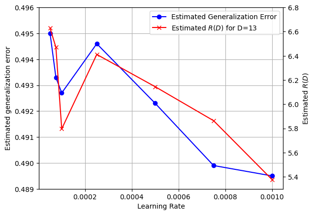
Figure 1: Estimated generalization error and rate-distortion values of the optimization trajectories of FCN4 trained with various learning rates.

V Experiments

In this section, we numerically verify the result of Theorem 7. As discussed in the previous work (e.g., [25]), $M$ cannot be estimated efficiently. Therefore, similar to those works, we ignore this term for the experimental part and study only the relation between the generalization error and $\mathfrak{RD}(S,\epsilon;\pi_{S})$. To study this relation, we follow the procedure below:

• We fix a dataset, a neural network, and all optimization hyperparameters, except the learning rate.

• For many learning rates, in the range of $[5e-5,1e-3]$, we train the neural network with the given datasets, and normalize and save the optimization trajectories.

• We estimate the generalization errors of the trained networks, each one trained with a different fixed learning rate, using the available “test set”.

• We estimate the rate-distortion values of the optimization trajectories of the trained networks, each one trained with a different fixed learning rate, using “Neural Estimator of the Rate-Distortion” (NERD) [77].

Fig 1 shows the plot of the results obtained from our experiments. The experiments are implemented over a fully connected network with 4 hidden layers (FCN4) architecture, trained using SGD and the dataset CIFAR10 [78]. The details of the experiments are given in the Appendix D. As it can be observed, the rate distortion estimation of the optimization trajectory follows the behavior of the generalization error to a relatively good extent.

The appendices are organized as follows:

• In Appendix A, we show that our rate-distortion theoretic bounds of Theorem 5 and Proposition 1 do not suffer from the limitations of the Xu-Ragisnsky bound as mentioned in [59].

• In Appendix B, we show how our framework can recover certain previous dimension-based results,

• In Appendix C, a simple corollary of the tail bound is presented.

• In Appendix D, we provide further the details about the experiments of Section V.

• Appendix E contains the proofs.

Appendix A $\mathcal{O}(1/n)$ Generalization Bounds for the Setup of [59]

Despite the popularity of PAC-Bayes and information-theoretic generalization bounds, their relevance and utility in practice are sometimes questioned. The recent works [59] and [79] argue that such bounds are not expressive enough generally and fail to give non-vacuous bounds in some cases. In what follows we show that the results of rate-distortion theoretic bounds of Theorem 5 and Proposition 1 escape those limitations. Specifically, for the setup considered in [59] we obtain in-expectation and PAC-Bayes generalization bounds for the considered that are not only non-vacuous but decay with $n$ as $\mathcal{O}(1/n)$.

We start by recalling the counter-example setup used in  [59] to infer that information-theoretic type bounds such as [2, 3] do fall short to explain generalization and expressiveness. The authors of [59] also provide a similar counter-example and arguments for conditional mutual information (CMI)-type bounds [4]. However, for reasons of brevity and compatibility with our framework we do not discuss them hereafter.

A-A Counter-example of [59]

Consider the following stochastic convex optimization (SCO) problem optimized using Gradient Descent (GD) as stated in [59].

Constants: Fix an $n\in\mathbb{N}$. Let $T_{n}=2n^{2}$, $\eta_{n}=\frac{1}{n\sqrt{5n}}$, $d_{n}=\frac{3}{4}T_{n}2^{n}$, and $\lambda_{n}=\frac{1}{n\sqrt{d}}$. In the rest of the section, we drop the dependencies (subscripts) on $n$ for a better readability.

Data distribution and training set. Let $\mathcal{Z}=\{0,1\}^{d}$. Let $\mathbf{Z}=(Z_{1},\ldots,Z_{d})\in\mathcal{Z}$ be a random vector whose elements are i.i.d. and distributed according to the Bernoulli$(1/2)$ distribution, i.e., $\mathbf{Z}\sim\text{Bern}(1/2)^{\otimes d}\eqqcolon\mu$. Denote the elements of the training dataset $S$ of size $n$ by

$$S=\{\mathbf{Z}_{1},\mathbf{Z}_{2},\ldots,\mathbf{Z}_{n}\}\sim\mu^{\otimes n},\quad\quad\mathbf{Z}_{i}=(Z_{i,1},Z_{i,2},\ldots,Z_{i,d})\in\mathcal{Z},i\in[n].$$

Hypothesis space and loss function. The hypothesis space $\mathcal{W}$ is the ball of radius 1 in $\mathbb{R}^{d}$ and the considered loss function $\ell\colon\mathcal{Z}\times\mathcal{W}\to\mathbb{R}^{+}$ is defined as

$$\ell(\mathbf{z},\mathbf{w})\coloneqq\sum_{j\in[d]}z_{j}w_{j}^{2}+\lambda\langle\mathbf{w},\mathbf{z}\rangle+\max\left\{\max_{j\in[d]}\left\{w_{j}\right\},0\right\},$$ (35)

where $\mathbf{z}=(z_{1},z_{2},\ldots,z_{d})\in\mathcal{Z}$ and $\mathbf{w}=(w_{1},w_{2},\ldots,w_{d})\in\mathcal{W}$.

Learning algorithm. The considered learning algorithm $\mathcal{A}\colon\mathcal{Z}^{n}\to\mathcal{W}$ is the output of the $T$ rounds of iterations of the Gradient Decent (GD) algorithm, initialized by $\mathbf{W}_{0}=\mathbf{0}\in\mathbb{R}^{d}$. More precisely, for $t\in[T]$, let

$$\mathbf{W}^{\{t+1\}}=\Pi_{\mathcal{W}}\left(\mathbf{W}^{\{t\}}-\eta\nabla\hat{\mathcal{L}}(S,\mathbf{W}^{\{t\}})\right),$$

where $\hat{\mathcal{L}}(S,\mathbf{W}^{\{t\}})=\frac{1}{n}\sum_{i\in[n]}\ell(\mathbf{Z}_{i},\mathbf{W}^{\{t\}})$ and $\Pi_{\mathcal{W}}\colon\mathbb{R}^{d}\to\mathcal{W}$ denotes the Euclidean projection operator, i.e.,

$$\Pi_{\mathcal{W}}(\mathbf{x})\coloneqq\operatorname*{arg\,min}_{\mathbf{W}\in\mathcal{W}}\|\mathbf{W}-\mathbf{x}\|_{2}=\frac{\mathbf{x}}{\max(\|\mathbf{x}\|_{2},1)}.$$

With the above notations, $\mathcal{A}(S)=\mathbf{W}^{\{T\}}$.

A-B $\mathcal{O}(1/n)$ Generalization Gap Bounds

In [59], the authors show that the Xu-Raginsky information-theoretic upper bound on the generalization error of [3] is loose and falls short to characterize the behavior of the generalization error for the aforementioned counter-example. This is obtained by showing that: (i) for every $\sigma>0$ it holds that [59, Theorem 4]

$$\sqrt{\frac{2I(S;\hat{\mathbf{W}})}{n}}+\mathbb{E}_{S}\left[\left|\mathcal{L}\left(\hat{\mathbf{W}}\right)-\mathcal{L}\left(\mathbf{W}^{\{T\}}\right)\right|\right]+\mathbb{E}_{S}\left[\left|\hat{\mathcal{L}}\left(S,\hat{\mathbf{W}}\right)-\mathcal{S}\left(S,\mathbf{W}^{\{T\}}\right)\right|\right]=\Omega(1)$$ (36)

where $\hat{\mathbf{W}}=\Pi_{\mathcal{W}}\left(\mathbf{W}^{\{T\}}+\xi\right)$, and $\xi\sim\mathcal{N}\left(0,\sigma^{2}\mathrm{I}_{d}\right)$; and (ii) that the true in-expectation generalization error satisfies

$$\mathbb{E}_{S}\left[\operatorname{gen}(S,\mathbf{W}^{\{T\}})\right]=\mathcal{O}\left(1/\sqrt{n}\right).$$ (37)

The authors also observe that considering a perturbation of the bound of [3] with an i.i.d. Gaussian noise $\xi$ does not resolve the issue. Furthermore, in [59, Theorem 9] they establish that when applied to the same counter-example the PAC-Bayes bounds of [30, 31] suffer from similar limitations.

In what follows, we show that our rate-distortion theoretic results of Theorem 5 and Proposition 1 lead to in-expectation and PAC-Bayes generalization bounds for the counter-example that are not only non-vacuous (by opposition to that of Xu-Raginsky [3]) but are tighter than the right hand side of (37). Specifically, application of our Theorem 5 yields that

$$\mathbb{E}_{S}\left[\operatorname{gen}\left(S,\mathbf{W}^{\{T\}}\right)\right]=\mathcal{O}\left(1/n\right);$$ (38)

and application of our Proposition 1 yields that for any fixed $\delta\geq 0$ (that does not grow with $n$), with probability at least $1-\delta$ over the choice of $S$, we have

$$\operatorname{gen}\left(S,\mathbf{W}^{\{T\}}\right)=\mathcal{O}\left(1/n\right).$$ (39)

The proofs of (38) and (39) can be found in Appendix E-I.

Appendix B Relation to dimension-based bounds

In this section, we show how using Theorem 3 we can recover certain dimension-based bounds, and in particular, [25, Theorem 2]. We state the assumptions used in [25, Theorem 2] in their simplest form. We refer the readers to [25] for further precision.

Şimşekli et al. [25] considered the continuous-time model of the SGD. Suppose that $U\in\mathcal{U}$ is the stochasticity of the algorithm, which is independent of $S$. Denote the deterministic output of the algorithm at time $t$, when $S=s$ and $U=u$, as $W_{s|u}^{t}\coloneqq\mathcal{A}(s,t|u)\in\mathbb{R}^{d}$. Denote $W_{s}^{t}\coloneqq W_{s|U}^{t}$, as a random variable representing the model at time $t$ for a given $s$, that depends on $U$. For any $u$ and $s$, denote $\mathcal{W}_{s|u}\coloneqq\{w\in\mathcal{W}\colon\exists t\in\mathsf{T},w=\mathcal{A}(s,t|u)\}$ as the support set of the trajectory of the hypotheses for a particular dataset $s$ and the stochasticity $u$. To recall, we assume the interval as $\mathsf{T}\coloneqq[0,1]\subseteq\mathbb{R}$ and denote the set of hypotheses along the trajectories by $W^{\mathsf{T}}$. Denote $\mathcal{W}_{s}\coloneqq\mathcal{W}_{s|U}$, as a random variable representing the random trajectory for a given $s$. To state their result, consider the collection of closed balls of radius $\epsilon$, with the centers on the fixed grid

$$\mathcal{N}_{\epsilon}\coloneqq\left\{\left(\frac{(2j_{1}+1)\epsilon}{2\sqrt{d}},\cdots,\frac{(2j_{d}+1)\epsilon}{2\sqrt{d}}\right)\colon j_{i}\in\mathbb{Z},i=1,\ldots,d\right\}.$$

For each $u$ and $s$, define the set $\mathcal{N}_{\epsilon}(s|u)\coloneqq\{x\in\mathcal{N}_{\epsilon}\colon B_{d}(x,\epsilon)\bigcap\mathcal{W}_{s|u}\neq\varnothing\}$, where $B_{d}(x,\epsilon)$ denotes the closed ball centered around $x\in\mathbb{R}^{d}$ with radius $\epsilon$. The following assumption is mainly used in their works.

Assumption 8 ([25, Definition 5])

Fix some $u\in\mathcal{U}$. Let $\mathcal{Z}^{\infty}\coloneqq(\mathcal{Z}\times\cdots\times\mathcal{Z})$ denote the countable product endowed with the product topology and let $\mathfrak{B}$ be the Borel $\sigma$-algebra generated by $\mathcal{Z}^{\infty}$. Let $\mathfrak{F},\mathfrak{G}$ be the $\sigma$-subalgebras of $\mathfrak{B}$ generated by the collection of random variables given by $\{\mathcal{\hat{L}}(s,w)\colon w\in\mathcal{W},n\geq 1\}$ and $\left\{\bm{1}\{w\in\mathcal{N}_{\epsilon}(s|u)\}\colon\delta\in\mathbb{Q}_{>0},w\in\mathcal{N}_{\epsilon},n\geq 1\right\}$. There exists a constant $M\geq 1$ such that for any $F\in\mathfrak{F}$ and $G\in\mathfrak{G}$, we have $\mathbb{P}(F\bigcap G)\leq M\mathbb{P}(F)\mathbb{P}(G)$.

The following result makes a connection between the generalization error and the Hausdorff dimensions ($\dim_{H}$) of the optimization trajectories. The result is established when this dimension coincides with the Minkowski dimension ($\dim_{M}$). For brevity, we refer the readers to [25, Definitions 2 & S3] for the definition of the Hausdorff and Minkowski dimensions.

Theorem 9 ([25, Theorem 2])

Suppose that the loss $\ell\colon\mathcal{Z}\times\mathcal{W}\to[0,1]$ is $\mathfrak{L}$-Lipschitz. Suppose that almost surely $\dim_{H}(W_{S|U})=\dim_{M}(W_{S|U})<\infty$. Then, under Assumption 8, with probability at least $1-\delta$,

$$\sup_{t\in[0,1]}|\operatorname{gen}(S,W^{t}_{S})|{=}\sup_{W\in\mathcal{W}_{S}}|\operatorname{gen}(S,W)|\leq 2\sqrt{\frac{(\dim_{H}(\mathcal{W}_{S|U})+1)\log^{2}(n\mathfrak{L}^{2})}{n}+\frac{\log(7M/\delta)}{n}}.$$

Now, we prove this result, using Theorem 3.i and more precisely using Corollary 1, that takes into account the stochasticity $U$.

Proof:

For each $s$ and $u$, denote the size of the set $\mathcal{N}_{\epsilon}(s|u)$ as $N_{\epsilon}(s|u)\coloneqq|\mathcal{N}_{\epsilon}(s|u)|$, which is bounded due to Assumption H2 of [25]. As it is shown in [25], for any $\delta^{\prime}>0$, there exists a set $\tilde{\mathcal{S}}\subseteq\mathcal{S}$ with probability at least $1-\delta^{\prime}$ such that for this set, $\epsilon\coloneqq 1/(n\mathfrak{L}^{2})$, and sufficiently large $n$,

$$\log N_{\epsilon}(S|U)\leq(\dim_{H}(\mathcal{W}_{S|U})+1)\log^{2}(n\mathfrak{L}^{2}).$$ (40)

Note that the results used in [25] are for $\epsilon\coloneqq 1/\sqrt{n\mathfrak{L}^{2}}$. However, their general expression for bounding $N_{\epsilon}(S|U)$ is not limited to that choice. Hence,

$$\mathbb{P} \left(\sup_{W\in\mathcal{W}_{S}}|\operatorname{gen}(S,W)|>2\sqrt{\frac{(\dim_{H}(\mathcal{W}_{S|U})+1)\log^{2}(n\mathfrak{L}^{2})}{n}+\frac{\log(7M/\delta)}{n}}\right)$$

$$\stackrel{{\scriptstyle(a)}}{{\leq}}\mathbb{P}\left(\sup_{W\in\mathcal{W}_{S}}|\operatorname{gen}(S,W)|>\sqrt{\frac{(\dim_{H}(\mathcal{W}_{S|U})+1)\log^{2}(n\mathfrak{L}^{2})+\log(4Mn/\delta)}{2n-1}+4\mathfrak{L}\epsilon}\right)$$

$$\leq\delta^{\prime}+\mathbb{P}\left(\sup_{W\in\mathcal{W}_{S}}|\operatorname{gen}(S,W)|>\sqrt{\frac{\log N_{\epsilon}(S|U)+\log(4Mn/\delta)}{2n-1}+4\mathfrak{L}\epsilon}\right),$$ (41)

where $(a)$ holds for $n$ sufficiently large and for $\epsilon\coloneqq 1/(n\mathfrak{L}^{2})$.

Let $\delta^{\prime}=\delta/2$. We show that the last term of (41) is bounded by $\delta/2$, which completes the proof. To do so, we use Corollary 1.i. and let $w\mapsto w^{\mathsf{T}}$ and $\delta\mapsto\delta/2$, $\epsilon\mapsto 4\mathfrak{L}\epsilon$,

$$f(s,w^{\mathsf{T}})\coloneqq\left(\sup_{t\in[0,1]}\operatorname{gen}(s,w^{t}_{s})\right)^{2},\quad\Delta(u,s)\coloneqq\frac{\log N_{\epsilon}(s|u)+\log(4Mn/\delta)}{2n-1}+4\mathfrak{L}\epsilon.$$

Let $\hat{\mathcal{W}}\coloneqq\mathcal{W}$ and $g(s,\hat{w})\coloneqq\operatorname{gen}(s,\hat{w})^{2}$. Note that $\forall w,\hat{w}\in\mathcal{W}$, we have $|\operatorname{gen}(s,w)-\operatorname{gen}(s,\hat{w})|\leq 4\mathfrak{L}\|w-\hat{w}\|$. Thus, for any given $s$ and $u$, and any $\nu_{u,s,w}\in\mathcal{F}_{U,S,W^{\mathsf{T}}}^{\delta}$, there exists at least one $\hat{w}\in\mathcal{N}_{\epsilon}(s|u)$, such that

$$g(s,\hat{w})+4\mathfrak{L}\epsilon\geq f(s,w_{[0:1]})\geq\Delta(u,s),$$

where the last inequality is deduced since $\nu_{u,s,w^{t}}\in\mathcal{F}^{\delta}_{U,S,W^{\mathsf{T}}}$. For any $s$ and $u$, denote such a set of $\hat{w}$ such that $g(s,\hat{w})+4\mathfrak{L}\epsilon\geq\Delta(u,s)$ as $\mathcal{N}^{*}_{\epsilon}(s|u)$. Then, let $p_{\hat{W}|U,S}$ be a deterministic (delta Dirac) distribution, picking one of the $\hat{w}\in\mathcal{N}^{*}_{\epsilon}(s|u)$. This choice of distribution satisfies the distortion criterion (46) with $\epsilon\mapsto 4\mathfrak{L}\epsilon$. Note that $\hat{W}$ and $W^{\mathsf{T}}$ are not of the same dimension. Moreover, $\hat{W}$ is a discrete random variable and deterministic given an $S=s$ and $U=u$. For any $s$ and $u$, let $q_{\hat{W}|U,S}$ be a uniform distribution over $\mathcal{N}^{*}_{\epsilon}(s|u)$. Now, for any $\nu_{u,s,w^{t}}\in\mathcal{F}^{\delta}_{U,S,W^{\mathsf{T}}}$,

$$D_{KL}\left(p_{\hat{W}|U,S}\nu_{U,S}\|q_{\hat{W}|U,S}\nu_{U,S}\right)= \mathbb{E}_{\nu_{U,S}}[\log N_{\epsilon}(S|U)].$$ (42)

Furthermore, with $\lambda\coloneqq(2n-1)$,

$$\log\mathbb{E}_{P_{U}P_{S}q_{\hat{W}|S}}\left[e^{\lambda g(S,\hat{W})}\right]\stackrel{{\scriptstyle(a)}}{{\leq}} \log\left(M\mathbb{E}_{P_{U}P_{S}q_{\hat{W}}}\left[e^{\lambda\operatorname{gen}(S,\hat{W})^{2}}\right]\right)$$

$$\leq \log(M)+\log\left(2n\right).$$ (43)

Relations (42) and (40) conclude that Condition (45) is satisfied for any $\nu_{u,s,w}$. This completes the proof. ∎

Another notable work showing a connection between generalization error and the intrinsic dimensions is by Camuto et al. [29]. They have studied the generalization error of the stochastic learning algorithms that can be expressed as random iterated function systems (IFS). In this case, and under mild conditions, they made a connection between the generalization error and the Hausdorff dimension of the induced invariant measure given $S$. Similar to the approach above, one can recover [29, Theorem 1]. Here, we avoid showing the steps, as heavy notations and definitions are needed to introduce the setup of that work.

Appendix C A corollary of the tail bound

As mentioned, if any random variable $U$ representing the (partial) stochasticity of the algorithm is known, the bound may be improved by making the sufficient conditions conditioned on $U$, in a similar way as in [24, Section D.2, Theorem 10]. Here, we state the result, whose proof follows from Theorem 3, by letting $S\mapsto U$ and $P_{S}\mapsto P_{S}P_{U}$.

Corollary 1

Suppose that $U\sim P_{U}$ represents the (partial) stochasticity of the algorithm, that is independent of $S$, i.e., the joint distribution of $(U,S,W)$ can be written as $P_{U,S,W}=P_{U}P_{S}P_{W|S,U}$. Let $f(S,W)\colon\mathcal{U}\times\mathcal{S}\times\mathcal{W}\to\mathbb{R}$ and $\Delta(U,S,W)\colon\mathcal{U}\times\mathcal{S}\times\mathcal{W}\to\mathbb{R}^{+}$. Fix arbitrarily the set $\hat{\mathcal{W}}$ and define arbitrarily $g(S,\hat{W})\colon\mathcal{U}\times\mathcal{S}\times\mathcal{\hat{W}}\to\mathbb{R}$. Then, for any $\delta\in\mathbb{R}^{+}$, with probability at least $1-\delta$,

$$f(S,W)\leq\Delta(U,S,W),$$ (44)

if any of these conditions hold:

• For some $\epsilon\in\mathbb{R}$ and any $\nu_{U,S,W}\in\mathcal{F}_{U,S,W}^{\delta}\coloneqq\mathcal{G}_{U,S,W}^{\delta}\bigcap\mathcal{S}_{U,S,W}\left(f(s,w)-\Delta(u,s,w)\right)$,

  $$\inf_{p_{\hat{W}|U,S}\in\mathcal{Q}(\nu_{U,S,W})}\inf_{\lambda>0,q_{\hat{W}|U,S}}\bigg{\{} \mathfrak{T}_{1,P_{U}P_{S}}(\nu_{U,S},p_{\hat{W}|U,S},q_{\hat{W}|U,S},\lambda g)$$

  $$-D_{KL}(\nu_{U,S,W}\|P_{W|U,S}\nu_{U,S})$$

  $${-}\lambda\left(\mathbb{E}_{\nu_{U,S,W}}\left[\Delta(U,S,W)\right]-\epsilon\right)\bigg{\}}\leq\log(\delta),$$ (45)

  where $\nu_{U,S}$ and $\nu_{S,W}$ are the marginal distributions of $(U,S)$ and $(S,W)$, respectively, under $\nu_{U,S,W}$ and $\mathcal{Q}(\nu_{U,S,W})$ is the set of all distributions $p_{\hat{W}|U,S}$ such that

  $$\mathbb{E}_{\nu_{U,S,W}p_{\hat{W}|U,S}}\left[\Delta(U,S,W)-g(S,\hat{W})\right]\leq\epsilon.$$ (46)

• For some $\alpha>1$ and any $\nu_{U,S,W}\in\mathcal{F}_{U,S,W}^{\delta}$,

  $$\inf_{q_{W|U,S},\lambda\geq\alpha/(\alpha-1)}\bigg{\{} \mathfrak{T}_{\alpha,P_{U}P_{S}}(\nu_{U,S},\nu_{W|U,S},q_{W|U,S},\lambda\log(f))-\lambda\left(\mathbb{E}_{\nu_{U,S}}\log\mathbb{E}_{\nu_{W|U,S}}\left[\Delta(U,S,W)\right]\right)\bigg{\}}\leq\log(\delta).$$ (47)

Appendix D Details of the Experiments

Here, we provide a detailed explanation of the experimental setup in Section V.

Tasks description

In our experiments, we followed the procedure, explained in Section V. Here, we repeat them and add more details in the following.

• We fix a dataset, a neural network, and all optimization hyperparameters, except the learning rate.

• For many learning rates, in the range of $[5e-5,1e-3]$, we train the neural network with the given dataset, and normalize and save the optimization trajectories.

• We estimate the generalization errors of the neural networks, each one trained with a different fixed learning rate, using the available “test set”.

• We estimate the rate-distortion values of the optimization trajectories of the trained networks, each one trained with a different fixed learning rate, using “Neural Estimator of the Rate-Distortion” (NERD) [77].

Datasets

To generate the optimization trajectories, we trained all models in a supervised manner and for the image classification task using the the dataset CIFAR10 [78]. CIFAR10 contains 10 classes of color images of size $32\times 32$. It contains $50000$ training images, that are used for training and also for measuring the empirical risk, and $10000$ test images, that are used to estimate the population risk.

Model

We considered a fully connected network with 4 hidden layers (FCN4) with the width $1024$. The total number of parameters is 18,894,848.

Training and hyperparameters

Training is performed using SGD with a fixed learning rate ($\eta$) in the range $[5e-5,1e-3]$ and a batch size of $50$. All models are trained until they reach a training accuracy of $100\%$ and a negative training log-likelihood of less than $5e-3$. The models are trained for another 10 epochs, during which the parameters of the models are first normalized and then stored. We normalize the weights to make it reasonable to compare the rate distortion values of different models trained with different learning algorithms. These stored models are used as a “dataset” in the next step, which measures their lossy compressibility for a given distortion level.

Measuring the rate-distortion values

We use the “Neural Estimator of the Rate-Distortion” (NERD) [77] to measure the lossy compressibility of the optimization trajectories. Due to the large size of the trained model, i.e., dataset with dimension 18,894,848, we choose a layer, randomly sample some of the neurons from the input and output of that layer, and choose all corresponding weights between them. Then we use NERD to measure the compressibility of this smaller dimension “dataset”. We repeat this process enough times for each layer, and the reported values are the average of the derived values.

Hardware and implementation

We performed our experiments on a server equipped with 56 CPUs Intel Xeon E5-2690v4 2.60GHz and 4 GPUs Nvidia Tesla P-100 PCIe 16GB.

Our implementations use the Python language and the deep learning framework PyTorch [80].

Appendix E Proofs

In this section, we provide the proofs of the results of the paper.

E-A Proof of Theorem 1

Proof:

For ease of notations, let $\mathcal{E}$ be the event that $\min_{j\leq e^{\sum_{i\in[m]}R_{S_{i},W_{i}}}}d_{m}(W^{m},\hat{\mathbf{w}}[j];S^{m})>\epsilon$ and $\mathcal{E}^{C}$ be its complement. For any $\nu\in(0,\log(1/\delta))$, let $m_{0}$ be sufficiently large such that for any $m\geq m_{0}$, $\mathbb{P}_{(S,W)^{\otimes m}}\left(\mathcal{E}\right)\leq e^{-m(\log(1/\delta)-\nu)}$. Let $\Delta(S,W)\coloneqq\frac{4\sigma^{2}(R_{S,W}+\log(\sqrt{2n}/\delta))}{2n-1}+\epsilon$. Then,

$$\mathbb{P}_{(S,W)}\Big{(}\operatorname{gen}(S,W)>\sqrt{\Delta(S,W)}\Big{)}^{m}$$

$$=\mathbb{P}_{(S,W)^{\otimes m}}\Big{(}\forall i\in[m]\colon\operatorname{gen}(S_{i},W_{i})^{2}>\Delta(S_{i},W_{i})\Big{)}$$

$$\leq\mathbb{P}_{(S,W)^{\otimes m}}\bigg{(}\frac{1}{m}\sum_{i\in[m]}\operatorname{gen}(S_{i},W_{i})^{2}>\frac{1}{m}\sum_{i\in[m]}\Delta(S_{i},W_{i})\bigg{)}$$

$$\leq\mathbb{P}_{(S,W)^{\otimes m}}\bigg{(}\frac{1}{m}\sum_{i\in[m]}\operatorname{gen}(S_{i},W_{i})^{2}>\frac{1}{m}\sum_{i\in[m]}\Delta(S_{i},W_{i}),\mathcal{E}^{C}\bigg{)}+\mathbb{P}_{(S,W)^{\otimes m}}(\mathcal{E})$$

$$\leq\mathbb{P}_{(S,W)^{\otimes m}}\bigg{(}\frac{1}{m}\sum_{i\in[m]}\operatorname{gen}(S_{i},W_{i})^{2}>\frac{1}{m}\sum_{i\in[m]}\Delta(S_{i},W_{i}),\mathcal{E}^{C}\bigg{)}+e^{-m(\log(1/\delta)-\nu)}$$

$$\leq\mathbb{P}_{S^{\otimes m}}\bigg{(}\exists j\leq e^{\sum_{i\in[m]}R_{S_{i},W_{i}}}\colon\frac{1}{m}\sum_{i\in[m]}\operatorname{gen}(S_{i},\hat{w}_{i}[j])^{2}>\frac{1}{m}\sum_{i\in[m]}\Delta(S_{i},W_{i})-\epsilon\bigg{)}$$

$$\hskip 14.22636pt+e^{-m(\log(1/\delta)-\nu)}$$

$$\stackrel{{\scriptstyle(a)}}{{\leq}}\delta^{m}\log(e^{mR_{\max}+m\,\eta_{m}})+e^{-m(\log(1/\delta)-\nu)}$$

$$=\delta^{m}(mR_{\max}+m\,\eta_{m})+e^{-m(\log(1/\delta)-\nu)},$$ (48)

where $(a)$ is derived in the following for some sequence of $\eta_{m}$ such that $\lim_{m\rightarrow\infty}\eta_{m}=0$. The proof completes by taking the $m$’th root, and since $\nu$ can be chosen arbitrarily small.

Now, we show the step $(a)$:

$$\mathbb{P}_{S^{\otimes m}}\left(\exists j\leq e^{\Sigma_{i}R_{S_{i},W_{i}}}\colon\sum_{i}\operatorname{gen}(S_{i},\hat{w}_{i}[j])^{2}>4\sigma^{2}\sum_{i}\frac{R_{S_{i},W_{i}}+\log(\sqrt{2n}/\delta)}{2n-1}\right)$$

$$=\mathbb{P}_{S^{\otimes m}}\left(\exists j\leq e^{\Sigma_{i}R_{S_{i},W_{i}}}\colon\sum_{i}\operatorname{gen}(S_{i},\hat{w}_{i}[j])^{2}>4\sigma^{2}\frac{\sum_{i}R_{S_{i},W_{i}}+m\log(\sqrt{2n}/\delta)}{2n-1}\right)$$

$$\leq\mathbb{P}_{S^{\otimes m}}\left(\exists R\leq mR_{\max}\colon\exists j\leq e^{R}\colon\sum_{i}\operatorname{gen}(S_{i},\hat{w}_{i}[j])^{2}>4\sigma^{2}\frac{R+m\log(\sqrt{2n}/\delta)}{2n-1}\right)$$

$$\leq\mathbb{P}_{S^{\otimes m}}\left(\exists R\leq mR_{\max}\colon\exists j\leq e^{R}\colon\sum_{i}\operatorname{gen}(S_{i},\hat{w}_{i}[j])^{2}>4\sigma^{2}\frac{\log(j)+m\log(\sqrt{2n}/\delta)}{2n-1}\right)$$

$$=\mathbb{P}_{S^{\otimes m}}\left(\exists j\leq e^{mR_{\max}}\colon\sum_{i}\operatorname{gen}(S_{i},\hat{w}_{i}[j])^{2}>4\sigma^{2}\frac{\log(j)+m\log(\sqrt{2n}/\delta)}{2n-1}\right)$$

$$\leq\sum_{j\leq e^{mR_{\max}}}\mathbb{P}_{S^{\otimes m}}\left(\sum_{i}\operatorname{gen}(S_{i},\hat{w}_{i}[j])^{2}>4\sigma^{2}\frac{\log(j)+m\log(\sqrt{2n}/\delta)}{2n-1}\right)$$

$$\stackrel{{\scriptstyle(a)}}{{\leq}}\sum_{j\leq e^{mR_{\max}}}e^{-\left(\log(j)+m\log(\sqrt{2n}/\delta)\right)}\mathbb{E}\left[e^{\frac{\sum_{i}\operatorname{gen}(S_{i},\hat{w}_{i}[j])^{2}}{4\sigma^{2}/(2n-1)}}\right]$$

$$\stackrel{{\scriptstyle(b)}}{{\leq}}\delta^{m}\sum_{j\leq e^{mR_{\max}}}\frac{1}{j}$$

$$\stackrel{{\scriptstyle(c)}}{{\leq}}\delta^{m}\log(e^{mR_{\max}+m\,\eta_{m}}),$$

where $(a)$ is derived using the Chernoff bound and $(b)$ is derived by using [81] and the fact that for each $i\in[m]$, $\operatorname{gen}(S_{i},\hat{w}_{i}[j])$ is $\sigma/\sqrt{n}$ subgaussian. More precisely, [81, Theorem 2.6.IV.] yields for any $i\in[m]$ and $\lambda\in[0,1)$,

$$\mathbb{E}\left[e^{\frac{\lambda\operatorname{gen}\left(S_{i},\hat{w}_{i}[j]\right)^{2}}{(2\sigma^{2}/n)}}\right]\leq\frac{1}{\sqrt{1-\lambda}}.$$

Now, letting $\lambda=\frac{2n-1}{2n}$, we drive that

$$\mathbb{E}\left[e^{\frac{\operatorname{gen}\left(S_{i},\hat{w}_{i}[j]\right)^{2}}{(4\sigma^{2}/(2n-1))}}\right]=\mathbb{E}\left[e^{\frac{\lambda\operatorname{gen}\left(S_{i},\hat{w}_{i}[j]\right)^{2}}{(2\sigma^{2}/n)}}\right]\leq\frac{1}{\sqrt{1-\lambda}}=\sqrt{2n}.$$

Lastly, $(c)$ holds for some sequence of $\eta_{m}$ such that $\lim_{m\rightarrow\infty}\eta_{m}=0$ since the Harmonic series $H_{r}$ can upper bounded by $\log(r)+0.6+1/2r$. ∎

E-B Proof of Theorem 2

We present two proofs. To show the main elements of the proof, first, we give a simpler proof for the following simpler condition, which is more stringent than (12):

$$\inf_{p_{\hat{W}|S}\in\mathcal{Q}(\nu_{S,W})}\inf_{q_{\hat{W}}}D_{KL}\left(p_{\hat{W}|S}\nu_{S}\|q_{\hat{W}}\nu_{S}\right)\leq\mathbb{E}_{\nu_{S,W}}[R_{S,W}].$$ (49)

Then, in the second proof, we show that Condition 12 is sufficient.

E-B1 First proof

Proof:

Let $Q_{m}$ be the empirical distribution of a sequence $(s^{m},w^{m})\in\mathcal{S}^{m}\times\mathcal{W}^{m}$; denoted as $\mathcal{T}_{m}(s^{m},w^{m})=Q_{m}$. This is known in information theory as the “type” of the sequence. Let

$$\mathcal{Q}_{m}\coloneqq\left\{Q_{m}\colon D_{KL}(Q_{m}\|P_{S,W})\leq\log(1/\delta)\right\}.$$

For any $m$, we first start by constructing proper hypothesis books $\mathcal{H}_{m,Q_{m}}$ for $Q_{m}\in\mathcal{Q}_{m}$, with elements $\mathcal{H}_{m,Q_{m}}=\{\hat{\mathbf{w}}_{Q_{m}}[j],j\in[l_{Q_{m}}]\}$ and the following property for $m$ sufficiently large: for every sequence $(s^{m},w^{m})$ such that $\mathcal{T}_{m}(s^{m},w^{m})=Q_{m}$, there exists at least one index $j\in[l_{Q_{m}}]$, such that $d_{m}(w^{m},\hat{\mathbf{w}}_{Q_{m}}[j];s^{m})\leq\epsilon+\nu_{2}$. Due to [82, Section 6.1.2, Lemma 1] (adapted for leaning algorithm setup in [24, Lemma 28]), for any $p_{\hat{W}|S}$ and $q_{\hat{W}}$ and $m$ sufficiently large, such hypothesis books exist with the size $l_{Q_{m}}=e^{mD_{KL}(p_{\hat{W}|S}Q_{m,S}\|q_{\hat{W}}Q_{m,S})}$, where $Q_{m,S}$ here denotes the marginal distribution of $S$ under $Q_{m,S}$, i.e., the empirical distribution of $s^{m}$.

We construct the hypothesis book $\mathcal{H}_{m}$ as $\mathcal{H}_{m}\coloneqq\bigcup_{Q_{m}\in\mathcal{Q}_{m}}\mathcal{H}_{m,Q_{m}}\bigcup\{\hat{\mathbf{w}}_{0}\}$, where $\hat{\mathbf{w}}_{0}\in\mathcal{\hat{W}}^{m}$ is an arbitrary (dummy) vector. We now index elements of $\mathcal{H}_{m}$ in a proper manner to satisfy the compressibility condition (11). Let $r\coloneqq|\mathcal{Q}_{m}|$, which is upper bounded by $m^{|\mathcal{S}|\times|\mathcal{W}|}$, and consider an arbitrary ordering $\pi(Q_{m})\colon\mathcal{Q}_{m}\to[r]$ (with its inverse denoted as $\pi^{-1}(i)$, $i\in[r]$) for elements of $Q_{m}\in\mathcal{Q}_{m}$. Then, we let $\mathcal{H}_{m}=\{\hat{\mathbf{w}}[rj_{1}+j_{2}],j_{2}\in[r-1],j_{1}\leq e^{mR_{\max}}/r-1\}$, where $\hat{\mathbf{w}}[rj_{1}+j_{2}]\coloneqq\hat{\mathbf{w}}_{\pi^{-1}(j_{2})}[j_{1}]$, if $|\pi^{-1}(j_{2})|\leq j_{1}$, and otherwise $\hat{\mathbf{w}}[rj_{1}+j_{2}]\coloneqq\hat{\mathbf{w}}_{0}$. Hence, for any distribution $Q_{m}$, it is sufficient to consider only the first $r\times|\mathcal{H}_{Q_{m}}|$ elements of $\mathcal{H}_{m}$, which for sufficiently large $m$ can be bounded as

$$r\times|\mathcal{H}_{Q_{m}}| \leq m^{|\mathcal{S}|\times|\mathcal{W}|}\times e^{mD_{KL}(p_{\hat{W}|S}Q_{m,S}\|q_{\hat{W}}Q_{m,S})}\stackrel{{\scriptstyle(a)}}{{\leq}}e^{m(D_{KL}(p_{\hat{W}|S}Q_{m,S}\|q_{\hat{W}}Q_{m,S})+\nu_{1})}$$

$$\stackrel{{\scriptstyle(b)}}{{\leq}}e^{mE_{Q_{m,S}}[R_{S}+\nu_{1}]}\stackrel{{\scriptstyle(c)}}{{=}}e^{m(\sum_{i}R_{S_{i},W_{i}}+\nu_{1})},$$

where $(a)$ holds for sufficiently large $m$, $(b)$ by the assumptions of the theorem, and $(c)$ holds when $S^{m}$ has the empirical distribution $Q_{m,S}$. Now,

$$\mathbb{P}_{(S,W)^{\otimes m}} \left(\min_{j\leq e^{\sum_{i\in[m]}R_{S_{i},W_{i}}+\nu_{1}}}d(W^{m},\hat{\mathbf{w}}[j];S^{m})>\epsilon+\nu_{2}\right)$$

$$\leq \mathbb{P}_{(S,W)^{\otimes m}}\left(\min_{j\leq e^{\sum_{i\in[m]}R_{S_{i},W_{i}}+\nu_{1}}}d(W^{m},\hat{\mathbf{w}}[j];S^{m})>\epsilon+\nu_{2},\mathcal{T}(S^{m},W^{m})\in\mathcal{Q}_{m}\right)$$

$$+\mathbb{P}_{(S,W)^{\otimes m}}\left(\mathcal{T}(S^{m},W^{m})\notin\mathcal{Q}_{m}\right)$$

$$\stackrel{{\scriptstyle(a)}}{{\leq}} P_{(S^{m},W^{m})}\left(\mathcal{T}(S^{m},W^{m})\notin\mathcal{Q}_{m}\right)$$

$$\stackrel{{\scriptstyle(b)}}{{\leq}} (\delta+\eta_{m})^{m},$$

where $(a)$ holds for sufficiently large values of $m$ and by the hypothesis book construction described above, $(b)$ holds for $\lim_{m}\eta_{m}\to 0$ by using [51, Theorem 11.1.4] and since the number of possible empirical distributions of $(s^{m},w^{m})$ is polynomial with respect to $m$. This completes the proof. ∎

E-B2 Second proof

Now, we proceed to show that the condition (12) is sufficient. To this end, we use the random coding technique, commonly used in information theory [51], for constructing the hypothesis book. For each $\nu_{S,W}$, fix some $p_{\hat{W}|S,\nu_{S,W}}\in\mathcal{Q}(\nu_{S,W})$ and $q_{\hat{W},\nu_{S,W}}$. We show that the algorithm is $(R_{S,W}+\nu_{1},\epsilon+\nu_{2},\sigma;d_{m})$-compressible if (12) holds with these choices. The result then follows. For better readability, we drop the dependence on $\nu_{S,W}$, although it is assumed throughout the proof.

Define the set $\mathcal{Q}_{m}$ as in the first proof. With a slight abuse of notations, we write $\mathcal{T}(s^{m})\in\mathcal{Q}_{m}$, for a sequence $s^{m}$, if there exists a sequence $w^{m}$, such that $\mathcal{T}(s^{m},w^{m})\in\mathcal{Q}_{m}$. Moreover, if $\mathcal{T}(s^{m},w^{m})=Q_{m}$, we write $\mathcal{T}(s^{m})=Q_{m,S}$ and $\mathcal{T}(w^{m}|s^{m})=Q_{m,W|S}$.

For each sequence $(s^{m},w^{m})$, with empirical distribution $Q_{m}\in\mathcal{Q}_{m}$, we first construct the random hypothesis book $\mathcal{H}_{m,Q_{m}}=\{\hat{\mathbf{W}}_{Q_{m}}[j],j\in[l_{Q_{m}}]\}$, where

$$l_{Q_{m}}\coloneqq e^{m\mathbb{E}_{(S,W)\sim Q_{m}}[R_{S,W}]+m\nu_{1}/2}=e^{\sum_{i\in[m]}R_{s_{i},w_{i}}+\nu_{1}/2}.$$ (50)

For each $\mathcal{H}_{m,Q_{m}}$, generate in an i.i.d. manner, each $\hat{\mathbf{W}}_{Q_{m}}[j]$ according to $q_{\hat{W}}^{\otimes m}$. We construct the random $\mathcal{H}_{m}$ by proper concatenation of $\mathcal{H}_{m}\coloneqq\bigcup_{Q_{m}\in\mathcal{Q}_{m}}\mathcal{H}_{m,Q_{m}}\bigcup\{\hat{\mathbf{w}}_{0}\}$, and indexing them as explained in the first proof. Consider $m$ is sufficiently large, such that $m^{|\mathcal{S}|\times|\mathcal{W}|}\leq e^{m\nu_{1}/2}$. Now, in the way that the elements of $\mathcal{H}_{m}$ are indexed, as explained in the first proof, for each $(s^{m},w^{m})$ such that $\mathcal{T}(s^{m})\in\mathcal{Q}_{m}$, it is sufficient to consider the first $e^{\sum_{i\in[m]}R_{s_{i},w_{i}}+\nu_{1}}$ elements.

Note that so far, we have a random hypothesis book $\mathcal{H}_{m}$. In the following, we evaluate the probability of covering failure, i.e., LHS of (11), among all these randomly generated hypothesis books. By showing that this probability is asymptotically less than $\delta+\nu_{3}$, for any $\nu_{3}>0$ that is less than $\nu_{1}/2$, we conclude that there exists at least one proper $\mathcal{H}_{m}$ having such property. The proof completes then by noting that $\nu_{3}$ can be made arbitrarily small.

Now, denoting the probability among all hypothesis books by the subscript $\mathcal{H}_{m}$, we have

$$\mathbb{P}_{(S,W)^{\otimes m},\mathcal{H}_{m}}\left(\min_{j\leq e^{\sum_{i\in[m]}R_{S_{i},W_{i}}}}d(W^{m},\hat{\mathbf{W}}[j];S^{m})>\epsilon+\nu_{2}\right)$$

$$\hskip 5.69046pt\leq\mathbb{P}_{(S,W)^{\otimes m},\mathcal{H}_{m}}\left(\min_{j\leq e^{\sum_{i\in[m]}R_{S_{i},W_{i}}+\nu_{1}}}d(W^{m},\hat{\mathbf{W}}[j];S^{m})>\epsilon+\nu_{2},\mathcal{T}(S^{m},W^{m})\in\mathcal{Q}_{m}\right)$$

$$\hskip 17.07182pt+\mathbb{P}_{(S,W)^{\otimes m},\mathcal{H}_{m}}\left(\mathcal{T}(S^{m},W^{m})\notin\mathcal{Q}_{m}\right)$$

$$\hskip 5.69046pt\stackrel{{\scriptstyle(a)}}{{\leq}}\mathbb{P}_{(S,W)^{\otimes m},\mathcal{H}_{m}}\left(\min_{j\leq e^{\sum_{i\in[m]}R_{S_{i},W_{i}}+\nu_{1}}}d(W^{m},\hat{\mathbf{W}}[j];S^{m})>\epsilon+\nu_{2},\mathcal{T}(S^{m},W^{m})\in\mathcal{Q}_{m}\right)$$ (51)

$$\hskip 19.91684pt+(\delta+\eta_{m})^{m},$$

where $(a)$ follows similarly as the first proof. In the rest of the proof, we show that the first term (51), denoted as $P_{1}$, can be upper bounded by $e^{-m\nu_{3}}$ as $m\rightarrow\infty$, for any $\nu_{3}>0$ that is smaller than $\nu_{1}/2$. This completes the proof.

The term $P_{1}$ can be upper bounded as

$$P_{1}\leq\sum_{s_{m}\colon\mathcal{T}(s^{m})\in\mathcal{Q}_{m}}P_{S^{\otimes m}}(s^{m})\sum_{\begin{subarray}{c}Q_{m}\in\mathcal{Q}_{m}\end{subarray}}\mathbb{P}_{(W|S)^{\otimes m}}(\mathcal{T}(s^{m},W^{m})=Q_{m})\times P_{2},$$ (52)

where

$$P_{2}\coloneqq\mathbb{P}_{\mathcal{H}_{m},W^{m}}\left(\min_{j\leq e^{\sum_{i\in[m]}R_{s_{i},W_{i}}+\nu_{1}}}d(W^{m},\hat{\mathbf{W}}[j];s^{m})>\epsilon+\nu_{2}\Big{|}\mathcal{T}(s^{m},w^{m})\in Q_{m}\right).$$ (53)

We continue by analyzing $P_{2}$ for any $w^{m}$, such that $\mathcal{T}(s^{m},w^{m})=Q_{m}$.

Then,

$$\mathbb{P}_{\mathcal{H}_{m}} \left(\min_{j\leq e^{\sum_{i\in[m]}R_{s_{i},w_{i}}+\nu_{1}}}d(w^{m},\hat{\mathbf{W}}[j];s^{m})>\epsilon+\nu_{2}\right)$$

$$\leq\mathbb{P}_{\mathcal{H}_{m,Q_{m}}}\left(\min_{j\leq e^{\sum_{i\in[m]}R_{s_{i},w_{i}}+\nu_{1}/2}}d(w^{m},\hat{\mathbf{W}}_{Q_{m}}[j];s^{m})>\epsilon+\nu_{2}\right)$$

$$\leq\sum_{j\in e^{\sum_{i\in[m]}R_{s_{i},w_{i}}+\nu_{1}/2}}\mathbb{P}_{\mathcal{H}_{m,Q_{m}}}\left(d(w^{m},\hat{\mathbf{W}}_{Q_{m}}[j];s^{m})>\epsilon+\nu_{2}\right)$$

$$\stackrel{{\scriptstyle(a)}}{{\leq}}e^{\sum_{i\in[m]}R_{s_{i},w_{i}}+\nu_{1}/2}e^{-mD_{KL}(p_{\hat{W}|S}Q_{m,S}\|q_{\hat{W}}Q_{m,S})}$$

$$=e^{m\mathbb{E}_{Q_{m}}[R_{S,W}+\nu_{1}/2]}e^{-mD_{KL}(p_{\hat{W}|S}Q_{m,S}\|q_{\hat{W}}Q_{m,S})},$$

where $(a)$ holds by [51, Theorem 11.1.4] and due to the way $\mathcal{H}_{m,Q_{m}}$ is constructed and since $p_{\hat{W}|S}$ satisfies the distortion criterion (13).

Now, Combining this with (52) and (53), and since

$$\mathbb{P}_{(W|S)^{\otimes m}}(\mathcal{T}(s^{m},W^{m})=Q_{m})\leq e^{-mD_{KL}(Q_{m}\|P_{W|S}Q_{m,S})},$$

by [51, Theorem 11.1.4], we conclude that

$$P_{1}\leq m^{|\mathcal{S}|\times|\mathcal{W}|}e^{m\mathbb{E}_{Q_{m}}[R_{S,W}+\nu_{1}/2]}e^{-mD_{KL}(p_{\hat{W}|S}Q_{m,S}\|q_{\hat{W}}Q_{m,S})}e^{-mD_{KL}(Q_{m}\|P_{W|S}Q_{m,S})}$$

$$\leq e^{-m\nu_{3}},$$ (54)

where the last step holds for any $\nu_{1}/2>\nu_{3}>0$, given that $m$ is sufficiently large, due to Condition 11.

E-C Proof of Theorem 3

Proof:

E-C1 Part i.

We start the proof by showing a potentially-data-dependent version of the [24, Lemma 24], tailored for the stochastic learning setup. The lemma is proved in Appendix E-J.

Lemma 1

For any $\delta>0$,

$$\log\mathbb{P}\left(f(S,W)>\Delta(S,W)\right)\leq\max\bigg{(}\log(\delta),$$ (55)

$$\sup_{\nu_{S,W}\in\mathcal{F}_{S,W}^{\delta}}\inf_{p_{\hat{W}|S}\in\mathcal{Q}(\nu_{S,W})}\inf_{\lambda\geq 0}\left\{-D_{KL}(\nu_{S,W}\|P_{S,W})-\lambda\left(\mathbb{E}_{\nu_{S,W}}[\Delta(S,W)]-\epsilon-\mathbb{E}_{\nu_{S}P_{\hat{W}|S}}\left[g(S,\hat{W})\right]\right)\right\}\bigg{)}.$$

In the rest, we show that for any $\nu_{S,W}$, $p_{\hat{W}|S}$, $\lambda\geq 0$, and $q_{\hat{W}|S}$, we have

$$-D_{KL}(\nu_{S,W}\|P_{S,W})+\lambda\mathbb{E}_{\nu_{S}P_{\hat{W}|S}}\left[g(S,\hat{W})\right]\leq D_{KL}\left(p_{\hat{W}|S}\nu_{S}\|q_{\hat{W}|S}\nu_{S}\right)+\log\mathbb{E}_{P_{S}q_{\hat{W}|S}}\left[e^{\lambda g(S,\hat{W})}\right]$$

$$-D_{KL}(\nu_{S,W}\|P_{W|S}\nu_{S}).$$ (56)

This inequality and Lemma 1 complete the proof of the theorem. To show this inequality, for any $S=s$, using the Donsker-Varadhan inequality, we have

$$\lambda\mathbb{E}_{P_{\hat{W}|S=s}}\left[g(s,\hat{W})\right]\leq D_{KL}\left(P_{\hat{W}|S=s}\|q_{\hat{W}|S=s}\right)+\log\mathbb{E}_{q_{\hat{W}|S=s}}\left[e^{\lambda g(s,\hat{W})}\right].$$

Next, taking the expectation with respect to $\nu_{S}$, gives

$$\lambda\mathbb{E}_{\nu_{S}P_{\hat{W}|S}}\left[g(S,\hat{W})\right] \leq D_{KL}\left(P_{\hat{W}|S}\nu_{S}\|q_{\hat{W}|S}\nu_{S}\right)+\mathbb{E}_{\nu_{S}}\log\left(\mathbb{E}_{q_{\hat{W}|S}}\left[e^{\lambda g(S,\hat{W})}\right]\right)$$

$$\stackrel{{\scriptstyle(a)}}{{\leq}}D_{KL}\left(P_{\hat{W}|S}\nu_{S}\|q_{\hat{W}|S}\nu_{S}\right)+D_{KL}(\nu_{S}\|P_{S})+\log\mathbb{E}_{P_{S}}\left[\mathbb{E}_{q_{\hat{W}|S}}\left[e^{\lambda g(S,\hat{W})}\right]\right],$$ (57)

where $(a)$ is derived by using the Donsker-Varadhan inequality. The desired inequality (56) can be derived from (57). This completes the proof.

E-C2 Part ii.

To show this part, we first establish a lemma similar to Lemma 1, proved in Appendix E-K.

Lemma 2

For any $\alpha>1$ and $\delta>0$,

$$\log\mathbb{P}\left(f(S,W)>\Delta(S,W)\right)\leq\max\Bigg{(}\log(\delta),$$ (58)

$$\sup_{\nu_{S,W}\in\mathcal{F}_{S,W}^{\delta}}\inf_{\lambda\geq 0}\left\{-D_{KL}(\nu_{S,W}\|P_{S,W})-\lambda\mathbb{E}_{\nu_{S}}\left[\log\mathbb{E}_{\nu_{W|S}}[\Delta(S,W)]-\log\mathbb{E}_{\nu_{W|S}}\left[f(S,W)\right]\right]\right\}\Bigg{)}.$$

Now, for $\lambda\geq 1/C_{\alpha}$ where $C_{\alpha}\coloneqq(\alpha-1)/\alpha$, we have

$$\lambda\mathbb{E}_{\nu_{S}}\left[\log\mathbb{E}_{\nu_{W|S}}\left[f(S,W)\right]\right]= \frac{\lambda C_{\alpha}}{C_{\alpha}}\mathbb{E}_{\nu_{S}}\left[\log\mathbb{E}_{\nu_{W|S}}\left[f(S,W)\right]\right]$$

$$\stackrel{{\scriptstyle(a)}}{{\leq}} \frac{1}{C_{\alpha}}\mathbb{E}_{\nu_{S}}\left[\log\mathbb{E}_{\nu_{W|S}}\left[f(S,W)^{\lambda C_{\alpha}}\right]\right]$$

$$\stackrel{{\scriptstyle(b)}}{{\leq}} \frac{1}{C_{\alpha}}\mathbb{E}_{\nu_{S}}\left[C_{\alpha}D_{\alpha}\left(\nu_{W|S}\|q_{W|S}\right)+C_{\alpha}\log\mathbb{E}_{q_{W|S}}\left[f(S,W)^{\frac{\lambda C_{\alpha}}{C_{\alpha}}}\right]\right]$$

$$\leq \mathbb{E}_{\nu_{S}}\left[D_{\alpha}\left(\nu_{W|S}\|q_{W|S}\right)\right]+D_{KL}(\nu_{S}\|P_{S})+\log\mathbb{E}_{P_{S}q_{W|S}}\left[f(S,W)^{\lambda}\right]$$

$$= \mathbb{E}_{\nu_{S}}\left[D_{\alpha}\left(\nu_{W|S}\|q_{W|S}\right)\right]+D_{KL}(\nu_{S,W}\|P_{S,W})$$

$$-D_{KL}(\nu_{S,W}\|P_{W|S}\nu_{S})+\log\mathbb{E}_{P_{S}q_{W|S}}\left[f(S,W)^{\lambda}\right],$$

where $(a)$ is due to convexity of the function $x^{r}$ for $r\geq 1$, and $(b)$ by the generalization of the Donsker-Varadhan inequality [83]. The proof completes by using Lemma 2. ∎

E-D Proof of Theorem 4

Proof:

Denote

$$\mathcal{A}_{S}\coloneqq\Big{\{}s\in\mathcal{S}\,\big{|}\,\exists\pi\colon\mathbb{E}_{W\sim\pi}\left[f(s,W)\right]>\Delta(s,\pi)\Big{\}}.$$

Consider a learning algorithm $P_{W|S}$ defined as follows: if $s\in\mathcal{A}_{S}$, then let $P_{W|S=s}$ be any distribution $\pi_{s}$ such that $\mathbb{E}_{W\sim\pi_{s}}\left[f(s,W)\right]>\Delta(s,\pi_{s})$, otherwise choose $P_{W|S=s}$ as any arbitrary distribution. Then, we have

$$\mathbb{P}_{S}\left(\exists\pi:\mathbb{E}_{W\sim\pi}\left[f(S,W)\right]>\Delta(S,\pi)\right)=\mathbb{P}_{S}\left(\mathbb{E}_{W\sim P_{W|S}}\left[f(S,W)\right]>\Delta(S,P_{W|S})\right).$$

Hence, it is sufficient to show the RHS is less than $\delta$, given that (by assumptions of the theorem) any of these conditions hold:

• For any distribution $\nu_{S}\in\mathcal{F}_{S}^{\delta}\coloneqq\mathcal{G}_{S}^{\delta}\bigcap\mathcal{S}_{S}\left(\mathbb{E}_{W\sim P_{W|S}}[f(s,W)]-\Delta(s,P_{W|S})\right)$,

  $$\log(\delta)\geq\inf_{p_{\hat{W}|S}\in\mathcal{Q}(\nu_{S}P_{W|S})}\inf_{q_{\hat{W}|S},\lambda>0}\bigg{\{} \mathfrak{T}_{1,P_{S}}(\nu_{S},p_{\hat{W}|S},q_{\hat{W}|S},\lambda g)-\lambda\left(\mathbb{E}_{\nu_{S}}\left[\Delta(S,P_{W|S})\right]-\epsilon\right)\bigg{\}},$$ (59)

  where $\mathcal{Q}(\nu_{S}P_{W|S})$ contains all the distributions $p_{\hat{W}|S}$ such that

  $$\mathbb{E}_{\nu_{S}p_{\hat{W}|S}}\left[\Delta(S,P_{W|S})-g(S,\hat{W})\right]\leq\epsilon.$$

• For $\alpha>1$ and any distribution $\nu_{S}\in\mathcal{F}_{S}^{\delta}$,

  $$\inf_{q_{W|S},\lambda\geq\alpha/(\alpha-1)}\bigg{\{} \mathfrak{T}_{\alpha,P_{S}}(\nu_{S},P_{W|S},q_{W|S},\lambda\log(f)-\lambda\mathbb{E}_{\nu_{S}}\left[\log\Delta(S,P_{W|S})\right]\bigg{\}}\leq\log(\delta),$$

We show the proof of each case separately.

• Applying Lemma 1 with $f(S,W)\mapsto\mathbb{E}_{P_{W|S}}\left[f(S,W)\right]$ and $\Delta(S,W)\mapsto\Delta(S,P_{W|S})$ (note that both terms depend only on $S$) gives

  $$\log\mathbb{P}\left(\mathbb{E}_{P_{W|S}}\left[f(S,W)\right]\geq\Delta(S,P_{W|S})\right)\leq\max\Bigg{(}\log(\delta),$$

  $$\sup_{\nu_{S}\in\mathcal{F}_{S}^{\delta}}\inf_{p_{\hat{W}|S}\in\mathcal{Q}(\nu_{S}P_{W|S})}\inf_{\lambda\geq 0}\left\{-D_{KL}(\nu_{S}\|P_{S})-\lambda\left(\mathbb{E}_{\nu_{S}}[\Delta(S,P_{W|S})]-\epsilon-\mathbb{E}_{\nu_{S}p_{\hat{W}|S}}\left[g(S,\hat{W})\right]\right)\right\}\Bigg{)}.$$

  The rest of the proof follows similarly to the proof of part i. of Theorem 3 to upper bound the term $\lambda\mathbb{E}_{\nu_{S}p_{\hat{W}|S}}\left[g(S,\hat{W})\right]$.

• Applying Lemma 2 with $f(S,W)\mapsto\mathbb{E}_{P_{W|S}}\left[f(S,W)\right]$ and $\Delta(S,W)\mapsto\Delta(S,P_{W|S})$ (note that both terms depend only on $S$) gives

  $$\log\mathbb{P}\Big{(}\mathbb{E}_{P_{W|S}} \left[f(S,W)\right]\geq\Delta(S,P_{W|S})\Big{)}\leq\max\Bigg{(}\log(\delta),$$

  $$\sup_{\nu_{S}\in\mathcal{F}_{S}^{\delta}}\inf_{\lambda\geq 0}\left\{-D_{KL}(\nu_{S}\|P_{S})-\lambda\mathbb{E}_{\nu_{S}}\left[\log\Delta(S,P_{W|S})-\log\mathbb{E}_{P_{W|S}}\left[f(S,W)\right]\right]\right\}\Bigg{)}.$$

  The rest of the proof follows similarly to the proof of part ii. of Theorem 3 to bound $\lambda\mathbb{E}_{\nu_{S}}\left[\log\mathbb{E}_{P_{W|S}}\left[f(S,W)\right]\right]$.

∎

E-E Proof of Theorem 5

E-E1 Part i.

Proof:

First, note that

$$\mathbb{E}_{(S,W)\sim P_{S,W}}\left[f(S,W)\right]\leq\mathbb{E}_{(S,\hat{W})\sim P_{S}p_{\hat{W}|S}}\left[g(S,\hat{W})\right]+\epsilon.$$ (60)

Now, using the Donsker-Varadhan inequality, for any $p_{\hat{W}|S}$, $\lambda\geq 0$, and $q_{\hat{W}|S}$, we have

$$\lambda\mathbb{E}_{P_{S}p_{\hat{W}|S}}\left[g(S,\hat{W})\right]\leq D_{KL}\left(p_{\hat{W}|S}P_{S}\|q_{\hat{W}|S}P_{S}\right)+\log\mathbb{E}_{P_{S}q_{\hat{W}|S}}\left[e^{\lambda g(S,\hat{W})}\right].$$ (61)

Combining this inequality and inequality (60) completes the proof. ∎

E-E2 Part ii.

Proof:

Using the generalization of the Donsker-Varadhan inequality [83], for any $\lambda\geq 1/C_{\alpha}$, where $C_{\alpha}\coloneqq(\alpha-1)/\alpha$, and $q_{W|S}$, we have

$$\lambda\log\mathbb{E}_{P_{S,W}}\left[f(S,W)\right]= \frac{\lambda C_{\alpha}}{C_{\alpha}}\log\mathbb{E}_{P_{S,W}}\left[f(S,W)\right]$$

$$\leq \frac{1}{C_{\alpha}}\log\mathbb{E}_{P_{S,W}}\left[f(S,W)^{\lambda C_{\alpha}}\right]$$

$$\leq \frac{1}{C_{\alpha}}\left[C_{\alpha}D_{\alpha}\left(P_{S,W}\|q_{W|S}P_{S}\right)+C_{\alpha}\log\mathbb{E}_{P_{S}q_{W|S}}\left[f(S,W)^{\frac{\lambda C_{\alpha}}{C_{\alpha}}}\right]\right].$$

This completes the proof. ∎

E-F Proof of Proposition 1

Proof:

The proof of part i. follows immediately from part i. of Theorem 4. To show the second part, we use part i. of Theorem 3. For each $\nu_{S,W}\in\mathcal{F}_{S,W}^{\delta}$, consider $p_{\hat{W}|S}$ as the induced conditional distribution under $\nu_{S,W}p_{\hat{W}|S,W}$, where $p_{\hat{W}|S,W}$ satisfies $p_{\hat{W}|S,W}=p_{\hat{W}|W}$. Let $\lambda=1$ and $\Delta(S,W)$ be the right hand side of part ii. Then, we have

$$\mathfrak{T}_{1,P_{S}}(\nu_{S},p_{\hat{W}|S},q_{\hat{W}|S},\lambda g){-}D_{KL}(\nu_{S,W}\|P_{W|S}\nu_{S}){-}\lambda\left(\mathbb{E}_{\nu_{S,W}}\left[\Delta(S,W)\right]-\epsilon\right)$$

$$\hskip 2.84544pt\leq\mathbb{E}_{\nu_{S}}\left[D_{KL}\left(p_{\hat{W}|S}\|q_{\hat{W}|S}\right)\right]-D_{KL}(\nu_{S,W}\|P_{W|S}\nu_{S})-\mathbb{E}_{\nu_{S,W}p_{\hat{W}|W}}\left[\log\left(\frac{\mathrm{d}p^{*}_{\hat{W}|S}}{\mathrm{d}q_{\hat{W}|S}}\right)\right]{+}\log(\delta)$$

$$\hskip 2.84544pt\stackrel{{\scriptstyle(a)}}{{\leq}}\mathbb{E}_{\nu_{S}}\left[D_{KL}\left(p_{\hat{W}|S}\|q_{\hat{W}|S}\right)-D_{KL}(p_{\hat{W}|S}\|p^{*}_{\hat{W}|S})\right]-\mathbb{E}_{\nu_{S,W}p_{\hat{W}|W}}\left[\log\left(\frac{\mathrm{d}p^{*}_{\hat{W}|S}}{\mathrm{d}q_{\hat{W}|S}}\right)\right]+\log(\delta)$$

$$\hskip 2.84544pt=\mathbb{E}_{\nu_{S}p_{\hat{W}|S}}\left[\log\left(\frac{\mathrm{d}p^{*}_{\hat{W}|S}}{\mathrm{d}q_{\hat{W}|S}}\right)\right]-\mathbb{E}_{\nu_{S,W}p_{\hat{W}|W}}\left[\log\left(\frac{\mathrm{d}p^{*}_{\hat{W}|S}}{\mathrm{d}q_{\hat{W}|S}}\right)\right]+\log(\delta)$$

$$\hskip 2.84544pt=\log(\delta),$$ (62)

where $(a)$ is deduced from the data processing inequality. This completes the proof. ∎

E-G Proof of Theorem 6

Proof:

We use Theorem 4 to prove the result. Let

$$f(s,w^{\mathsf{T}}) \coloneqq\operatorname{gen}(S,W^{\mathsf{T}})=\frac{1}{\Delta t}\sum_{t\in\mathsf{T}}\operatorname{gen}(s,w^{t}),$$

$$\Delta(\pi) \coloneqq\sqrt{\frac{\sup_{\nu_{s}\in\mathcal{G}^{\delta}_{S}}\mathfrak{RD}(\nu_{S},\epsilon;\pi)+\log(1/\delta)}{2n}}+\epsilon.$$

Let $\mathcal{\hat{W}}\subseteq\mathcal{W}$ and $g(s,\hat{w}^{\mathsf{T}})=f(s,\hat{w}^{\mathsf{T}})$. Now, consider any arbitrary distributions $\pi_{S}$, index by $S$, and any $\nu_{S}\in\mathcal{F}_{S}^{\delta}$. Consider any $p_{\hat{W}^{\mathsf{T}}|S}$ such that

$$\mathbb{E}_{\nu_{S}\pi_{S}p_{\hat{W}^{\mathsf{T}}|S}}\left[f(S,W^{\mathsf{T}})-f(S,\hat{W}^{\mathsf{T}})\right]\leq\epsilon.$$

Since $\nu_{S}\in\mathcal{F}_{S}^{\delta}$, then $p_{\hat{W}^{\mathsf{T}}|S}$ satisfies the distortion criterion (25). Let $q_{\hat{W}^{\mathsf{T}}|S}\coloneqq q_{\hat{W}^{\mathsf{T}}}$ be the marginal distribution of $\hat{W}^{\mathsf{T}}$ under $p_{\hat{W}^{\mathsf{T}}|S}\nu_{S}$. Then, LHS of Condition 24 becomes as

$$\inf_{p_{\hat{W}^{\mathsf{T}}|S},q_{\hat{W}^{\mathsf{T}}},\lambda>0}\bigg{\{}I_{\nu_{s}p_{\hat{W}^{\mathsf{T}}|S}}(S;\hat{W}^{\mathsf{T}})-\lambda\big{(}\mathbb{E}_{\nu_{S}} \left[\Delta(\pi_{S})\right]-\epsilon\big{)}+\log\mathbb{E}_{P_{S}q_{\hat{W}^{\mathsf{T}}}}\left[e^{\lambda f(S,\hat{W}^{\mathsf{T}})}\right]\bigg{\}}$$

$$\stackrel{{\scriptstyle(a)}}{{\leq}} \inf_{\lambda>0}\bigg{\{}\mathfrak{RD}(\nu_{S},\epsilon;\pi_{S})-\lambda\left(\Delta(\pi_{S})-\epsilon\right)+\frac{\lambda^{2}}{8n}\bigg{\}}$$

$$\stackrel{{\scriptstyle(b)}}{{=}} \mathfrak{RD}(\nu_{S},\epsilon;\pi_{S})-\sup_{\nu_{s}\in\mathcal{G}^{\delta}_{S}}\mathfrak{RD}(\nu_{S},\epsilon;\pi_{S})-\log(1/\delta)$$

$$\leq \log(\delta)$$ (63)

where $(a)$ is concluded since $f(S,\hat{w}^{\mathsf{T}})$ is $1/(2\sqrt{n})$-subgaussian and $(b)$ is derived for $\lambda\coloneqq 4n(\Delta(\pi_{S})-\epsilon)$. This completes the proof of part i. ∎

E-H Proof of Theorem 7

Proof:

We use Theorem 4 with $\epsilon\mapsto 4\mathfrak{L}\epsilon$ to prove the result. Let

$$f(s,w^{\mathsf{T}}) \coloneqq\operatorname{gen}(S,W^{\mathsf{T}})^{2}=\left(\frac{1}{\Delta t}\sum_{t\in\mathsf{T}}\operatorname{gen}(s,w^{t})\right)^{2},$$

$$\Delta(s,\pi) \coloneqq\frac{\mathfrak{RD}(s,\epsilon;\pi)+\log(\sqrt{2n}M/\delta)}{2n-1}+4\mathfrak{L}\epsilon.$$

Let $\mathcal{\hat{W}}\subseteq\mathcal{W}$ and $g(s,\hat{w}^{\mathsf{T}})=f(s,\hat{w}^{\mathsf{T}})$. Theorem 4 remains valid, if instead of all $\pi$, we limit ourselves to only one distribution $P_{W^{\mathsf{T}}|S}$, that we denote for the ease of exposition as $\pi_{S}$. Consider any $\nu_{S}\in\mathcal{F}_{S}^{\delta}$. For any $s\in\operatorname{supp}(\nu_{S})$, first let $p_{\hat{W}^{\mathsf{T}}|W^{\mathsf{T}},s}$ be any distribution that satisfies

$$\mathbb{E}_{\pi_{s}p_{\hat{W}^{\mathsf{T}}|W^{\mathsf{T}},s}}\left[\rho(W^{\mathsf{T}},\hat{W}^{\mathsf{T}})\right]\leq\epsilon.$$

In the following, for simplicity, we denote by $Q$, any (possibly marginal) distribution induced by $\nu_{S}\pi_{S}p_{\hat{W}^{\mathsf{T}}|W^{\mathsf{T}},S}$, e.g., $Q_{W^{\mathsf{T}},\hat{W}^{\mathsf{T}}}$ is the marginal distribution of $(W^{\mathsf{T}},\hat{W}^{\mathsf{T}})$ under the joint mentioned distribution. Note that

$$\mathbb{E}_{Q_{W^{\mathsf{T}},\hat{W}^{\mathsf{T}}}}\left[\rho(W^{\mathsf{T}},\hat{W}^{\mathsf{T}})\right]= \mathbb{E}_{\nu_{S}}\mathbb{E}_{\pi_{s}p_{\hat{W}^{\mathsf{T}}|W^{\mathsf{T}},s}}\left[\rho(W^{\mathsf{T}},\hat{W}^{\mathsf{T}})\right]\leq\epsilon.$$ (64)

Now define another distribution, denoted by $\tilde{Q}$, as any (possibly marginal) distribution induced by $\nu_{S}\pi_{S}\tilde{p}_{\hat{W}^{\mathsf{T}}|W^{\mathsf{T}},S}$, where $\tilde{p}_{\hat{W}^{\mathsf{T}}|W^{\mathsf{T}},S}\coloneqq Q_{\hat{W}^{\mathsf{T}}|W^{\mathsf{T}}}$. Note that $S\mathrel{\multimap}\joinrel\mathrel{-}\joinrel\mathrel{\mkern-6.0mu}\joinrel\mathrel{-}W^{\mathsf{T}}\mathrel{\multimap}\joinrel\mathrel{-}\joinrel\mathrel{\mkern-6.0mu}\joinrel\mathrel{-}\hat{W}^{\mathsf{T}}$ forms a Markov chain under $\tilde{Q}$, i.e., $\tilde{Q}_{\hat{W}^{\mathsf{T}}|W^{\mathsf{T}},S}=\tilde{Q}_{\hat{W}^{\mathsf{T}}|W^{\mathsf{T}}}$. Furthermore, $\tilde{Q}_{W^{\mathsf{T}},\hat{W}^{\mathsf{T}}}\coloneqq Q_{W^{\mathsf{T}},\hat{W}^{\mathsf{T}}}$.

Now,

$$\mathbb{E}_{\nu_{S}\tilde{Q}_{\hat{W}^{\mathsf{T}}|S}}\bigg{[}\Delta(S,\pi_{S})-\operatorname{gen}(S,\hat{W}^{\mathsf{T}})^{2}\bigg{]}\stackrel{{\scriptstyle(a)}}{{\leq}} \mathbb{E}_{\nu_{S}\tilde{Q}_{\hat{W}^{\mathsf{T}}|S}}\left[\mathbb{E}_{\pi_{S}}\left[\operatorname{gen}(S,W^{\mathsf{T}})^{2}\right]-\operatorname{gen}(S,\hat{W}^{\mathsf{T}})^{2}\right]$$

$$= \mathbb{E}_{\nu_{S}\pi_{S}\tilde{Q}_{\hat{W}^{\mathsf{T}}|S,W^{\mathsf{T}}}}\left[\operatorname{gen}(S,W^{\mathsf{T}})^{2}-\operatorname{gen}(S,\hat{W}^{\mathsf{T}})^{2}\right]$$

$$= \mathbb{E}_{\tilde{Q}_{S,W^{\mathsf{T}},\hat{W}^{\mathsf{T}}}}\left[\operatorname{gen}(S,W^{\mathsf{T}})^{2}-\operatorname{gen}(S,\hat{W}^{\mathsf{T}})^{2}\right]$$

$$\leq \mathbb{E}_{\tilde{Q}_{S,W^{\mathsf{T}},\hat{W}^{\mathsf{T}}}}\left[\big{|}\operatorname{gen}(S,W^{\mathsf{T}})^{2}-\operatorname{gen}(S,\hat{W}^{\mathsf{T}})^{2}\big{|}\right]$$

$$\stackrel{{\scriptstyle(b)}}{{\leq}} 2\mathbb{E}_{\tilde{Q}_{S,W^{\mathsf{T}},\hat{W}^{\mathsf{T}}}}\left[\big{|}\operatorname{gen}(S,W^{\mathsf{T}})-\operatorname{gen}(S,\hat{W}^{\mathsf{T}})\big{|}\right]$$

$$\stackrel{{\scriptstyle(c)}}{{\leq}} 4\mathfrak{L}\,\mathbb{E}_{\tilde{Q}_{S,W^{\mathsf{T}},\hat{W}^{\mathsf{T}}}}\left[\rho(W^{\mathsf{T}},\hat{W}^{\mathsf{T}})\right]$$

$$= 4\mathfrak{L}\,\mathbb{E}_{\tilde{Q}_{W^{\mathsf{T}},\hat{W}^{\mathsf{T}}}}\left[\rho(W^{\mathsf{T}},\hat{W}^{\mathsf{T}})\right]$$

$$\stackrel{{\scriptstyle(d)}}{{=}} 4\mathfrak{L}\,\mathbb{E}_{Q_{W^{\mathsf{T}},\hat{W}^{\mathsf{T}}}}\left[\rho(W^{\mathsf{T}},\hat{W}^{\mathsf{T}})\right]$$

$$\stackrel{{\scriptstyle(e)}}{{\leq}} 4\mathfrak{L}\epsilon,$$

where $(a)$ holds since $\nu_{S}\in\mathcal{F}_{S}^{\delta}$, $(b)$ due to the fact that $\ell(z,w)\in[0,1]$, $(c)$ by the Lipschitz assumption, $(d)$ is derived by noting that $Q_{W^{\mathsf{T}},\hat{W}^{\mathsf{T}}}=\tilde{Q}_{W^{\mathsf{T}},\hat{W}^{\mathsf{T}}}$, and $(e)$ due to (64).

Hence, $p_{\hat{W}^{\mathsf{T}}|S}\coloneqq\tilde{Q}_{\hat{W}^{\mathsf{T}}|S}$ is in the set $\mathcal{Q}(\nu_{S}\pi_{S})$, as defined in Theorem 4. Let $q_{\hat{W}^{\mathsf{T}}|S}\coloneqq q_{\hat{W}^{\mathsf{T}}}\coloneqq\tilde{Q}_{\hat{W}^{\mathsf{T}}}$. Note that $D_{KL}\left(p_{\hat{W}^{\mathsf{T}}|S}\nu_{S}\|q_{\hat{W}^{\mathsf{T}}|S}\nu_{S}\right)=I_{\tilde{Q}}(S;\hat{W}^{\mathsf{T}})$.

Now, restricting the inf in LHS of Condition 24 to only such choices described above, the LHS can be upper bounded as

LHS $$\leq\inf_{p_{\hat{W}^{\mathsf{T}}|S},q_{\hat{W}^{\mathsf{T}}}\lambda>0}\bigg{\{}I_{\tilde{Q}}(S;\hat{W}^{\mathsf{T}})-\lambda\left(\mathbb{E}_{\nu_{S}}\left[\Delta(S,\pi_{S})\right]-4\mathfrak{L}\epsilon\right)+\log\mathbb{E}_{P_{S}q_{\hat{W}^{\mathsf{T}}}}\left[e^{\lambda f(S,\hat{W}^{\mathsf{T}})}\right]\bigg{\}}$$

$$\stackrel{{\scriptstyle(a)}}{{\leq}}\inf_{p_{\hat{W}^{\mathsf{T}}|S},q_{\hat{W}^{\mathsf{T}}}}\bigg{\{}I_{\tilde{Q}}(S;\hat{W}^{\mathsf{T}})-(2n-1)\left(\mathbb{E}_{\nu_{S}}\left[\Delta(S,\pi_{S})\right]-4\mathfrak{L}\epsilon\right)+\log(\sqrt{2n})\bigg{\}}$$

$$\stackrel{{\scriptstyle(b)}}{{\leq}}\inf_{p_{\hat{W}^{\mathsf{T}}|S},q_{\hat{W}^{\mathsf{T}}}}\bigg{\{}I_{\tilde{Q}}(W^{\mathsf{T}};\hat{W}^{\mathsf{T}})-(2n-1)\left(\mathbb{E}_{\nu_{S}}\left[\Delta(S,\pi_{S})\right]-4\mathfrak{L}\epsilon\right)+\log(\sqrt{2n})\bigg{\}}$$

$$\stackrel{{\scriptstyle(c)}}{{=}}\inf_{p_{\hat{W}^{\mathsf{T}}|S},q_{\hat{W}^{\mathsf{T}}}}\bigg{\{}I_{Q}(W^{\mathsf{T}};\hat{W}^{\mathsf{T}})-(2n-1)\left(\mathbb{E}_{\nu_{S}}\left[\Delta(S,\pi_{S})\right]-4\mathfrak{L}\epsilon\right)+\log(\sqrt{2n})\bigg{\}}$$

$$\stackrel{{\scriptstyle(d)}}{{\leq}}\inf_{p_{\hat{W}^{\mathsf{T}}|S},q_{\hat{W}^{\mathsf{T}}}}\bigg{\{}I_{Q}(W^{\mathsf{T}};S,\hat{W}^{\mathsf{T}})-(2n-1)\left(\mathbb{E}_{\nu_{S}}\left[\Delta(S,\pi_{S})\right]-4\mathfrak{L}\epsilon\right)+\log(\sqrt{2n})\bigg{\}}$$

$$\stackrel{{\scriptstyle(e)}}{{=}}\inf_{p_{\hat{W}^{\mathsf{T}}|S},q_{\hat{W}^{\mathsf{T}}}}\bigg{\{}I_{Q}(W^{\mathsf{T}};\hat{W}^{\mathsf{T}}|S)+I_{Q}(W^{\mathsf{T}};S)-(2n-1)\left(\mathbb{E}_{\nu_{S}}\left[\Delta(S,\pi_{S})\right]-4\mathfrak{L}\epsilon\right)+\log(\sqrt{2n})\bigg{\}}$$

$$\leq\mathbb{E}_{\nu_{S}}\left[\mathfrak{RD}(S=s,\epsilon;\pi_{S=s})\right]+I_{Q}(W^{\mathsf{T}};S)-(2n-1)\left(\mathbb{E}_{\nu_{S}}\left[\Delta(S,\pi_{S})\right]-4\mathfrak{L}\epsilon\right)+\log(\sqrt{2n})$$

$$=\log(\delta)+\mathbb{E}_{\nu_{S},\pi_{S}}\left[\log\frac{\mathrm{d}\pi_{S}}{\mathrm{d}[\pi_{S}\nu_{S}]_{W^{\mathsf{T}}}}\right]-\mathbb{E}_{\nu_{S}}\left[\sup_{\nu\in\mathcal{G}_{S}^{\delta}}\mathbb{E}_{\pi_{S}}\log\frac{\mathrm{d}\pi_{S}}{\mathrm{d}[\pi_{S}\nu]_{W^{\mathsf{T}}}}\right]$$

$$\leq\log(\delta),$$ (65)

where $\mathrm{d}[\pi_{S}\nu]_{W^{\mathsf{T}}}$ (similarly for $\nu_{S}$) denotes the marginal distribution of $W^{\mathsf{T}}$ under $\pi_{S}\nu$,

• holds for $\lambda\coloneqq 2n-1$ and since for each $\hat{w}^{\mathsf{T}}$, $\operatorname{gen}(S,\hat{w}^{\mathsf{T}})$ is $1/(2\sqrt{n})$-subgaussian, and hence $\mathbb{E}\left[e^{(2n-1)f(S,\hat{w}^{\mathsf{T}})}\right]\leq\sqrt{2n}$ due to [81, Theorem 2.6.IV.],

• is due to the data processing inequality by using the fact that under $\tilde{Q}$, $S\mathrel{\multimap}\joinrel\mathrel{-}\joinrel\mathrel{\mkern-6.0mu}\joinrel\mathrel{-}W^{\mathsf{T}}\mathrel{\multimap}\joinrel\mathrel{-}\joinrel\mathrel{\mkern-6.0mu}\joinrel\mathrel{-}\hat{W}^{\mathsf{T}}$ forms a Markov chain,

• is deduced, since the marginal distributions of $(W^{\mathsf{T}},\hat{W}^{\mathsf{T}})$ is the same under $Q$ and $\tilde{Q}$ by definition,

• holds by the data processing inequality,

• is derived by using the chain rule for mutual information.

This completes the proof. ∎

E-I Proofs of Equations (38) and (39)

E-I1 Proof of (38)

Proof:

We start by recalling some notations and lemmas defined and developed in [59]. Define $\mathbf{B}=(B_{1},B_{2},\ldots,B_{d})\in\{0,1\}^{d}$ as following: for $j\in[d]$, $B_{j}=1$ if and only if for all $i\in[n]$, $Z_{i,j}=0$. Otherwise, i.e., if at least for one $i\in[n]$, $Z_{i,j}=1$, $B_{j}=0$. Trivially, $B_{j}=1$ with probability $2^{-n}$. When $B_{j}=1$, we call that coordinate, a ‘bad’ coordinate. Let $\|\mathbf{B}\|_{0}=\sum_{j\in[d]}B_{j}$ denote the number of bad coordinates. Denote the ordered indices of the bad coordinates as $\mathcal{B}=\{i_{1},\ldots,i_{\|\mathbf{B}\|_{0}}\}\subseteq[d]$. As shown in [59, Equation (15)], we have

$$\mathbb{P}\left(T/2\leq\|\mathbf{B}\|_{0}\leq T\right)\geq 1-2e^{-T/36}.$$ (66)

By denoting $\hat{\mu}_{j}$ as the mean of coordinate $j$ of the samples of $S$, i.e., letting $\hat{\mu}_{j}\coloneqq\frac{1}{n}\sum_{i\in[n]}Z_{i,j}$, we can re-write the empirical risk for any $\mathbf{w}=(w_{1},w_{2},\ldots,w_{d})\in\mathcal{W}$ as

$$\hat{\mathcal{L}}(S,\mathbf{W})=\sum_{j\in[d]}\hat{\mu}_{j}w_{j}^{2}+\lambda\langle\hat{\mu},\mathbf{w}\rangle+\max\left\{\max_{j\in[d]}\{w_{j}\},0\right\},$$ (67)

where $\hat{\mu}=(\hat{\mu}_{1},\hat{\mu}_{2},\ldots,\hat{\mu}_{d})$.

Next, we state a lemma on the dynamics of GD, developed in [59], using the former results of [84, 85].

Lemma 3 ( [59, Lemma 18])

Under the event that $\{T/2\leq\|\mathbf{B}\|_{0}\leq T\}$,

$$\mathbf{W}_{j}^{\{T\}}=\begin{cases}\frac{\lambda}{2}\left(-1+\left(1-2\eta\hat{\mu}_{j}\right)^{T}\right),&\text{if }j\in[d]\setminus\mathcal{B},\\ -\eta,&\text{if }j\in\mathcal{B}.\end{cases}$$ (68)

Let $\mathcal{E}$ be a binary random variable which is equal to $0$ whenever $\{T/2\leq\|\mathbf{B}\|_{0}\leq T\}$, and equal to $1$, otherwise. Denote

$$v_{0}= \frac{\lambda}{2}\left(-1+(1-\eta)^{T}\right),$$

$$v_{1}= -\eta.$$

Fix a given $r\in[1-\frac{1}{n^{2}},1]$ and consider the following quantization law of $p_{\hat{\mathbf{W}}|S}$: if $\mathcal{E}=1$, then let

$$\hat{\mathbf{W}}=(\hat{W}_{1},\ldots,\hat{W}_{d})=\mathbf{0}\in\mathbb{R}^{d},$$ (69)

with probability one. Otherwise, i.e., if $\mathcal{E}=0$, then for each $j\in[d]$, if $\hat{\mu}_{j}=0$, then let

$$\hat{W}_{j}=\begin{cases}v_{0},&\text{with probability $r$},\\ v_{1},&\text{with probability $1-r$},\end{cases}$$ (70)

and if $\hat{\mu}_{j}>0$, then let $\hat{W}_{j}=v_{0}$ with probability one.

It can be easily verified that for every $\hat{\mathbf{w}}$, with positive probability under $P_{S}p_{\hat{\mathbf{W}}|S}$, and every $\mathbf{z}\in\mathcal{Z}$,

$$0\leq\ell(\mathbf{z},\hat{\mathbf{w}})<\frac{2}{5n}+\frac{1}{4n^{2}}\eqqcolon 2\sigma.$$ (71)

Let $q_{\hat{\mathbf{W}}|S}\coloneqq q_{\hat{\mathbf{W}}}$ be the marginal distribution of $P_{S}p_{\hat{\mathbf{W}}|S}$. Now, part i. of Theorem 5 with the above choices of $p_{\hat{\mathbf{W}}|S}$ and $q_{\hat{\mathbf{W}}|S}$ and with $g(S,\hat{\mathbf{W}})\coloneqq\operatorname{gen}(S,\hat{\mathbf{W}})$ and $\lambda\coloneqq n^{2}$, gives

$$\mathbb{E}_{S}[\operatorname{gen}(S,\mathbf{W}^{\{T\}})]\leq \frac{1}{\lambda}\mathbb{E}_{P_{S}}\Big{[}D_{KL}\big{(}p_{\hat{\mathbf{W}}|S}\|q_{\hat{\mathbf{W}}}\big{)}\Big{]}+\frac{1}{\lambda}\log\mathbb{E}_{P_{S}q_{\hat{\mathbf{W}}}}\Big{[}e^{\lambda\operatorname{gen}(S,\hat{\mathbf{W}})}\Big{]}+\epsilon$$

$$= \frac{1}{\lambda}I(S;\hat{\mathbf{W}})+\frac{1}{\lambda}\log\mathbb{E}_{P_{S}q_{\hat{\mathbf{W}}}}\Big{[}e^{\lambda\operatorname{gen}(S,\hat{\mathbf{W}})}\Big{]}+\epsilon$$

$$\leq \frac{1}{\lambda}I(S;\hat{\mathbf{W}})+\frac{\lambda\sigma^{2}}{2n}+\epsilon$$

$$\leq \frac{1}{\lambda}I(S;\hat{\mathbf{W}})+\frac{\lambda}{10n^{3}}+\epsilon$$

$$\leq \frac{1}{\lambda}\left(H(\mathcal{E})+d\,h_{b}\big{(}(1-r)2^{-n})\big{)}\right)+\frac{\lambda}{10n^{3}}+\epsilon$$

$$\leq \frac{1}{\lambda}\left(\frac{1}{18}T\log_{2}(e)e^{-T/36}+\frac{3}{4}(1-r)T(n+1-\log_{2}(1-r))\right)+\frac{\lambda}{10n^{3}}+\epsilon$$

$$= \left(\frac{1}{9}\log_{2}(e)e^{-T/36}+\frac{3}{2}(1-r)(n+1-\log_{2}(1-r))\right)+\frac{1}{10n}+\epsilon$$

$$= \mathcal{O}\left(\frac{1}{n}\right)+\epsilon,$$ (72)

where $h_{b}(x)=-x\log_{2}(x)-(1-x)\log_{2}(1-x)$ is the binary Shannon entropy that satisfies the inequality $h_{b}(x)\leq x(1-\log_{2}(x))$ and

$$\epsilon=\mathbb{E}_{S,\hat{\mathbf{W}}}\left[\operatorname{gen}(S,\mathbf{W}^{\{T\}})-\operatorname{gen}(S,\hat{\mathbf{W}})\right].$$ (73)

Hence, it remains to show that $\epsilon=\mathcal{O}\left(1/n\right)$. Re-write the distortion term as

$$\mathbb{E}_{S}\left[\operatorname{gen}\left(S,\mathbf{W}^{\{T\}}\right)-\operatorname{gen}(S,\hat{\mathbf{W}})\right]= \mathbb{E}_{S}\left[\mathcal{L}\left(\mathbf{W}^{\{T\}}\right)-\mathcal{L}(\hat{\mathbf{W}})\right]+\mathbb{E}_{S}\left[\hat{\mathcal{L}}(S,\hat{\mathbf{W}})-\hat{\mathcal{L}}\left(S,\mathbf{W}^{\{T\}}\right)\right].$$ (74)

Now, we bound each terms separately by $\mathcal{O}(1/n)$ which completes the proof. Denote $\hat{\mathbf{W}}=(\hat{W}_{1},\ldots,\hat{W}_{d})$.

$$\mathbb{E}_{S}\left[\mathcal{L}\left(\mathbf{W}^{\{T\}}\right)-\mathcal{L}(\hat{\mathbf{W}})\right]\leq \mathbb{P}\left(\mathcal{E}=0\right)\mathbb{E}_{S}\left[\mathcal{L}\left(\mathbf{W}^{\{T\}}\right)-\mathcal{L}(\hat{\mathbf{W}})\bigg{|}\mathcal{E}=0\right]+\mathbb{P}\left(\mathcal{E}=1\right)\mathbb{E}_{S}\left[\mathcal{L}\left(\mathbf{W}^{\{T\}}\right)-\mathcal{L}(\hat{\mathbf{W}})\bigg{|}\mathcal{E}=1\right]$$

$$\stackrel{{\scriptstyle(a)}}{{\leq}} \mathbb{P}\left(\mathcal{E}=0\right)\mathbb{E}_{S}\left[\mathcal{L}\left(\mathbf{W}^{\{T\}}\right)-\mathcal{L}(\hat{\mathbf{W}})\bigg{|}\mathcal{E}=0\right]+(4+2/n)e^{-T/36}$$

$$\leq \mathbb{E}_{S}\left[\mathcal{L}\left(\mathbf{W}^{\{T\}}\right)-\mathcal{L}(\hat{\mathbf{W}})\bigg{|}\mathcal{E}=0\right]+(4+2/n)e^{-T/36}$$

$$= \mathbb{E}_{S}\left[\mathbb{E}_{\mathbf{Z}\sim\mu}\left[\ell(\mathbf{Z},\mathbf{W}^{\{T\}})-\ell(\mathbf{Z},\hat{\mathbf{W}})\right]\bigg{|}\mathcal{E}=0\right]+(4+2/n)e^{-T/36}$$

$$\stackrel{{\scriptstyle(b)}}{{\leq}} \frac{1}{2}\sum_{j\in[d]\setminus\mathcal{B}}\mathbb{E}_{S}\left[(W_{j}^{\{T\}}-\hat{W}_{j})(W_{j}^{\{T\}}+\hat{W}_{j}+\lambda)\right]$$

$$+\frac{1}{2}\sum_{j\in\mathcal{B}}\mathbb{E}_{S}\left[(W_{j}^{\{T\}}-\hat{W}_{j})(W_{j}^{\{T\}}+\hat{W}_{j}+\lambda)\right]+(4+2/n)e^{-T/36}$$

$$\stackrel{{\scriptstyle(c)}}{{\leq}} \frac{\lambda^{2}}{4}\sum_{j\in[d]\setminus\mathcal{B}}\mathbb{E}_{S}\left[\left|\left(\left(1-2\eta\hat{\mu}_{j}\right)^{T}-\left(1-\eta\right)^{T}\right)\right]\right|+\frac{1}{2}\sum_{j\in\mathcal{B}}\eta^{2}+(4+2/n)e^{-T/36}$$

$$\leq \frac{\eta\lambda^{2}(T+1)}{2}\sum_{j\in[d]\setminus\mathcal{B}}\mathbb{E}_{S}\left[\left|\hat{\mu}_{j}-\frac{1}{2}\right|\right]+\frac{\eta^{2}}{2}\|\mathbf{B}\|_{0}+(4+2/n)e^{-T/36}$$

$$\stackrel{{\scriptstyle(d)}}{{\leq}} \frac{\eta\lambda^{2}(T+1)}{4\sqrt{n}}(d-\|\mathbf{B}\|_{0})\ +\frac{\eta^{2}}{2}\|\mathbf{B}\|_{0}+(4+2/n)e^{-T/36}$$

$$= \mathcal{O}\left(\frac{1}{n}\right),$$

where

• $(a)$ is concluded by using (66) and noting that $\ell(\mathbf{z},\mathbf{0})=0$ and $\ell(\mathbf{z},\mathbf{w})\in[0,2+1/n]$ for every $\mathbf{z}\in\mathcal{Z}$ and $\mathbf{w}\in\mathcal{W}$,

• $(b)$ is derived by using Lemma 3, by definition of the loss function $\ell(\mathbf{z},\mathbf{w})$, and by noting that the distortion is maximized for $r=1$,

• $(c)$ is obtained by Lemma 3,

• and $(d)$ by noting that $\mathbb{E}_{S}\left[\left|\hat{\mu}_{j}-\frac{1}{2}\right|\right]\leq\frac{1}{2\sqrt{n}}$.

Finally, for the second term of (74) we have

$$\mathbb{E}_{S} \left[\hat{\mathcal{L}}(S,\hat{\mathbf{W}})-\hat{\mathcal{L}}\left(S,\mathbf{W}^{\{T\}}\right)\right]$$

$$\leq \mathbb{P}\left(\mathcal{E}=0\right)\mathbb{E}_{S}\left[\hat{\mathcal{L}}(S,\hat{\mathbf{W}})-\hat{\mathcal{L}}\left(S,\mathbf{W}^{\{T\}}\right)\bigg{|}\mathcal{E}=0\right]+\mathbb{P}\left(\mathcal{E}=1\right)\mathbb{E}_{S}\left[\hat{\mathcal{L}}(S,\hat{\mathbf{W}})-\hat{\mathcal{L}}\left(S,\mathbf{W}^{\{T\}}\right)\bigg{|}\mathcal{E}=1\right]$$

$$\leq \mathbb{P}\left(\mathcal{E}=0\right)\mathbb{E}_{S}\left[\hat{\mathcal{L}}(S,\hat{\mathbf{W}})-\hat{\mathcal{L}}\left(S,\mathbf{W}^{\{T\}}\right)\bigg{|}\mathcal{E}=0\right]+(4+2/n)e^{-T/36}$$

$$\leq \mathbb{E}_{S}\left[\hat{\mathcal{L}}(S,\hat{\mathbf{W}})-\hat{\mathcal{L}}\left(S,\mathbf{W}^{\{T\}}\right)\bigg{|}\mathcal{E}=0\right]+(4+2/n)e^{-T/36}$$

$$= \mathbb{E}_{S}\left[\sum_{j\in[d]\setminus B}\hat{\mu}_{j}\left((\hat{W}_{j}-W^{\{T\}}_{j}\right)\left(\hat{W}_{j}+W^{\{T\}}_{j}+\lambda\right)\bigg{|}\mathcal{E}=0\right]+(4+2/n)e^{-T/36}$$

$$\leq \sum_{j\in[d]\setminus B}\mathbb{E}_{S}\left[\left|\left((\hat{W}_{j}-W^{\{T\}}_{j}\right)\left(\hat{W}_{j}+W^{\{T\}}_{j}+\lambda\right)\right|\bigg{|}\mathcal{E}=0\right]+(4+2/n)e^{-T/36}$$

$$\leq \frac{\lambda^{2}}{2}\sum_{j\in[d]\setminus\mathcal{B}}\mathbb{E}_{S}\left[\left|\left(\left(1-2\eta\hat{\mu}_{j}\right)^{T}-\left(1-\eta\right)^{T}\right)\right]\right|+(4+2/n)e^{-T/36}$$

$$\leq \eta\lambda^{2}(T+1)\sum_{j\in[d]\setminus\mathcal{B}}\mathbb{E}_{S}\left[\left|\hat{\mu}_{j}-\frac{1}{2}\right|\right]+(4+2/n)e^{-T/36}$$

$$\leq \frac{\eta\lambda^{2}(T+1)}{2\sqrt{n}}(d-\|\mathbf{B}\|_{0})\ +(4+2/n)e^{-T/36}$$

$$= \mathcal{O}\left(\frac{1}{n}\right).$$

∎

E-I2 Proof of (39)

Proof:

The proof of part ii. is similar to the first part, but using Proposition 1 instead of Theorem 5. In Proposition 1, let $f(S,\mathbf{W})\mapsto\lambda\operatorname{gen}(S,\mathbf{W}^{\{T\}})$, $g(S,\hat{\mathbf{W}})\mapsto\lambda\operatorname{gen}(S,\hat{\mathbf{W}})$, $\epsilon\mapsto\lambda\epsilon$. Moreover, let $\pi$ be a deterministic distribution induced by GD. With these choices, with probability at least $1-\delta$,

$$\operatorname{gen}(S,\mathbf{W}^{\{T\}})\leq\frac{1}{\lambda}D_{KL}\left(p_{\hat{\mathbf{W}}|S}\|q_{\hat{\mathbf{W}}|S}\right)+\frac{1}{\lambda}\log\mathbb{E}_{P_{S}q_{\hat{\mathbf{W}}|S}}\left[e^{\lambda\operatorname{gen}(S,\hat{\mathbf{W}})}\right]+\frac{1}{\lambda}\log{(1/\delta)}+\epsilon.$$ (75)

for any $q_{\hat{\mathbf{W}}|S}$ and any $p_{\hat{\mathbf{W}}|S}$ that should satisfy $\mathbb{E}_{p_{\hat{\mathbf{W}}|S}}\big{[}\operatorname{gen}(S,\mathbf{W}^{\{T\}})-\operatorname{gen}(S,\hat{\mathbf{W}})\big{]}\leq\epsilon$.

Now, we define $p_{\hat{\mathbf{W}}|S}$ and $q_{\hat{\mathbf{W}}|S}$. For a given $S$, if $\mathcal{E}=1$, then let $\hat{\mathbf{W}}=\mathbf{W}$ with probability one. In this case, $\epsilon=0$. Otherwise, if $\mathcal{E}=0$, choose the quantization rule as in part i, i.e., fix a given $r\in[1-\frac{1}{n^{2}},1]$ and for each $j\in[d]$, if $\hat{\mu}_{j}=0$, then let

$$\hat{W}_{j}=\begin{cases}v_{0},&\text{with probability $r$},\\ v_{1},&\text{with probability $1-r$},\end{cases}$$ (76)

and if $\hat{\mu}_{j}>0$, then let $\hat{W}_{j}=v_{0}$ with probability one. Similar to part i. (but without taking expectation with respect to $S$), it can be shown that $\epsilon=\mathcal{O}(1/n)$ in (75).

If $\mathcal{E}=1$, let $q_{\hat{\mathbf{W}}|S}$ be equal to a multi-variate Gaussian distribution $\mathcal{N}(0,\mathrm{I}_{d})$ defined over $\mathcal{W}$, denoted as $q_{\hat{\mathbf{W}},1}$. Note that since $0\leq\ell(\mathbf{z},\mathbf{w})\leq(2+1/n)$, hence, $\operatorname{gen}(S,\mathbf{W})\leq(2+1/n)$.

If $\mathcal{E}=0$, let $q_{\hat{\mathbf{W}}|S}$ be a binary distribution, denoted by $q_{\hat{\mathbf{W}},2}$, taking value $v_{1}$ with probability $(1-r)2^{-n}\eqqcolon q$, and taking value $v_{0}$ with probability $(1-q)$.

It remains to show that whenever $\mathcal{E}=0$, then for some $\lambda$,

$$\frac{1}{\lambda}D_{KL}\left(p_{\hat{\mathbf{W}}|S}\|q_{\hat{\mathbf{W}}|S}\right)+\frac{1}{\lambda}\log\mathbb{E}_{P_{S}q_{\hat{\mathbf{W}}|S}}\left[e^{\lambda\operatorname{gen}(S,\hat{\mathbf{W}})}\right]+\frac{1}{\lambda}\log(1/\delta)=\mathcal{O}(1/n).$$ (77)

Whenever $\mathcal{E}=0$, we have

$$D_{KL}\big{(}p_{\hat{\mathbf{W}}|S}\|q_{\hat{\mathbf{W}}|S}\big{)}+ \log\mathbb{E}_{P_{S}q_{\hat{\mathbf{W}}|S}}\left[e^{\lambda\operatorname{gen}(S,\hat{\mathbf{W}})}\right]$$

$$= D_{KL}\left(p_{\hat{\mathbf{W}}|S}\|q_{\hat{\mathbf{W}},2}\right)+\log\mathbb{E}_{P_{S}q_{\hat{\mathbf{W}}|S}}\left[e^{\lambda\operatorname{gen}(S,\hat{\mathbf{W}})}\right]$$

$$= D_{KL}\left(p_{\hat{\mathbf{W}}|S}\|q_{\hat{\mathbf{W}},2}\right)+\log\left(\mathbb{E}_{P_{S}q_{\hat{\mathbf{W}},2}}\left[\mathbbm{1}_{\{\mathcal{E}=0\}}e^{\lambda\operatorname{gen}(S,\hat{\mathbf{W}})}\right]+\mathbb{E}_{P_{S}q_{\hat{\mathbf{W}},1}}\left[\mathbbm{1}_{\{\mathcal{E}=1\}}e^{\lambda\operatorname{gen}(S,\hat{\mathbf{W}})}\right]\right)$$

$$\leq D_{KL}\left(p_{\hat{\mathbf{W}}|S}\|q_{\hat{\mathbf{W}},2}\right)+\log\left(\mathbb{E}_{P_{S}q_{\hat{\mathbf{W}},2}}\left[e^{\lambda\operatorname{gen}(S,\hat{\mathbf{W}})}\right]+2e^{\lambda(2+1/n)}e^{-T/36}\right)$$

$$\leq D_{KL}\left(p_{\hat{\mathbf{W}}|S}\|q_{\hat{\mathbf{W}}}\right)+\log\left(e^{\frac{\lambda^{2}\sigma^{2}}{2n}}+2e^{3\lambda-T/36}\right)$$

$$\leq \left(d-\|\mathbf{B}\|_{0}\right)\log\left(\frac{1}{1-q}\right)+\|\mathbf{B}\|_{0}r\log\left(\frac{r}{1-q}\right)+\|\mathbf{B}\|_{0}(1-r)\log\left(\frac{1-r}{q}\right)$$

$$+2\max\left(\frac{\lambda^{2}\sigma^{2}}{2n},3\lambda-T/36\right)+\mathcal{O}(1),$$

where $\sigma$ is defined in (71). Plugging this in (77) and letting $\lambda=n^{2}/60$ gives the desired result. Note that by considering only the case where $\mathcal{E}=0$, we showed (77) holds with probability $1-\delta-2e^{-T/36}$. Finally, observing that $2e^{-T/36}=o(1/n)$ terminates the proof of the equality. ∎

E-J Proof of Lemma 1

Proof:

Denote $\mathcal{B}\coloneqq\left\{(s,w)\in\operatorname{supp}(P_{S,W})\colon f(s,w)>\Delta(s,w)\right\}$. If $P_{S,W}(\mathcal{B})=0$, then the lemma is proved. Assume then $P_{S,W}(\mathcal{B})>0$. Consider the distribution $\nu_{S,W}$ such that for any $(s,w)\in\mathcal{B}$, $\nu_{S,W}(s,w)\coloneqq P_{S,W}(s,w)/P_{S,W}(\mathcal{B})$, and otherwise $\nu(s,w)\coloneqq 0$. Note that by definition $\nu_{S,W}\in\mathcal{S}_{S,W}\left(f(s,w)-\Delta(s,w)\right)$. Now, if $\nu_{S,W}\notin\mathcal{G}_{S,W}^{\delta}$, then $D_{KL}(\nu_{S,W}\|P_{S,W})\geq\log(1/\delta)$. Hence,

$$\log(1/\delta)\leq D_{KL}(\nu_{S,W}\|P_{S,W})=-\log(P_{S,W}(\mathcal{B}))=-\log\mathbb{P}\left(f(S,W)>\Delta(S,W)\right).$$

Thus, $\log\mathbb{P}\left(f(S,W)>\Delta(S,W)\right)\leq\log(\delta)$. This completes the proof of Lemma.

Otherwise, suppose that $\nu_{S,W}\in\mathcal{G}_{S,W}^{\delta}$, which yields $\nu_{S,W}\in\mathcal{F}_{S,W}^{\delta}$, due to the fact that $\nu_{S,W}\in\mathcal{S}_{S,W}\left(f(s,w)-\Delta(s,w)\right)$. Then, for this distribution and any $p_{\hat{W}|S}\in\mathcal{Q}(\nu_{S,W})$ we have

$$\mathbb{E}_{\nu_{S,W}p_{\hat{W}|S}}\left[\Delta(S,W)-g(S,\hat{W})\right]\leq\epsilon.$$ (78)

Hence, it is optimal to let $\lambda=0$ in (55) for this distribution. Thus,

$$\inf_{p_{\hat{W}|S}\in\mathcal{Q}(\nu_{S,W})}\inf_{\lambda\geq 0}\left\{-D_{KL}(\nu_{S,W}\|P_{S,W})-\lambda\left(\mathbb{E}_{\nu_{S,W}}[\Delta(S,W)]-\epsilon-\mathbb{E}_{\nu_{S}P_{\hat{W}|S}}\left[g(S,\hat{W})\right]\right)\right\}$$

$$=-D_{KL}(\nu_{S,W}\|P_{S,W})=\log(P_{S,W}(\mathcal{B}))=\log\mathbb{P}\left(f(S,W)>\Delta(S,W)\right).$$

This proves the inequality. ∎

E-K Proof of Lemma 2

Proof:

The proof is similar to the proof of Lemma 1. Here, we repeat it for the sake of completeness.

Denote $\mathcal{B}\coloneqq\left\{(s,w)\in\operatorname{supp}(P_{S,W})\colon f(s,w)>\Delta(s,w)\right\}$. If $P_{S,W}(\mathcal{B})=0$, then the lemma is proved. Assume then $P_{S,W}(\mathcal{B})>0$. Consider the distribution $\nu_{S,W}$ such that for any $(s,w)\in\mathcal{B}$, $\nu_{S,W}(s,w)\coloneqq P_{S,W}(s,w)/P_{S,W}(\mathcal{B})$, and otherwise $\nu(s,w)\coloneqq 0$. Note that by definition $\nu_{S,W}\in\mathcal{S}_{S,W}\left(f(s,w)-\Delta(s,w)\right)$. Now, if $\nu_{S,W}\notin\mathcal{G}_{S,W}^{\delta}$, then $D_{KL}(\nu_{S,W}\|P_{S,W})\geq\log(1/\delta)$. Hence,

$$\log(1/\delta)\leq D_{KL}(\nu_{S,W}\|P_{S,W})=-\log(P_{S,W}(\mathcal{B}))=-\log\mathbb{P}\left(f(S,W)>\Delta(S,W)\right).$$

Thus, $\log\mathbb{P}\left(f(S,W)>\Delta(S,W)\right)\leq\log(\delta)$. This completes the proof of Lemma.

Otherwise, suppose that $\nu_{S,W}\in\mathcal{G}_{S,W}^{\delta}$, which yields $\nu_{S,W}\in\mathcal{F}_{S,W}^{\delta}$, due to the fact that $\nu_{S,W}\in\mathcal{S}_{S,W}\left(f(s,w)-\Delta(s,w)\right)$. Then, for this distribution we have

$$\mathbb{E}_{\nu_{S}}\left[\log\mathbb{E}_{\nu_{W|S}}[\Delta(S,W)]-\log\mathbb{E}_{\nu_{W|S}}\left[f(S,W)\right]\right]\leq 0.$$ (79)

Hence, it is optimal to let $\lambda=0$ in (55) for this distribution. Thus,

$$\inf_{\lambda\geq 0}\left\{-D_{KL}(\nu_{S,W}\|P_{S,W})-\lambda\mathbb{E}_{\nu_{S}}\left[\log\mathbb{E}_{\nu_{W|S}}[\Delta(S,W)]-\log\mathbb{E}_{\nu_{W|S}}\left[f(S,W)\right]\right]\right\}$$

$$=-D_{KL}(\nu_{S,W}\|P_{S,W})=\log(P_{S,W}(\mathcal{B}))=\log\mathbb{P}\left(f(S,W)>\Delta(S,W)\right).$$

This proves the inequality.

∎

References

• [1] S. Shalev-Shwartz and S. Ben-David, Understanding machine learning: From theory to algorithms.   Cambridge University Press, 2014.
• [2] D. Russo and J. Zou, “Controlling bias in adaptive data analysis using information theory,” in Proceedings of the 19th International Conference on Artificial Intelligence and Statistics, ser. Proceedings of Machine Learning Research, A. Gretton and C. C. Robert, Eds., vol. 51.   Cadiz, Spain: PMLR, 09–11 May 2016, pp. 1232–1240.
• [3] A. Xu and M. Raginsky, “Information-theoretic analysis of generalization capability of learning algorithms,” Advances in Neural Information Processing Systems, vol. 30, 2017.
• [4] T. Steinke and L. Zakynthinou, “Reasoning about generalization via conditional mutual information,” in Proceedings of Thirty Third Conference on Learning Theory, ser. Proceedings of Machine Learning Research, J. Abernethy and S. Agarwal, Eds., vol. 125.   PMLR, 09–12 Jul 2020, pp. 3437–3452.
• [5] A. R. Esposito, M. Gastpar, and I. Issa, “Generalization error bounds via Rényi-, $f$-divergences and maximal leakage,” 2020.
• [6] Y. Bu, S. Zou, and V. V. Veeravalli, “Tightening mutual information-based bounds on generalization error,” IEEE Journal on Selected Areas in Information Theory, vol. 1, no. 1, p. 121–130, May 2020.
• [7] M. Haghifam, G. K. Dziugaite, S. Moran, and D. M. Roy, “Towards a unified information-theoretic framework for generalization,” in Thirty-Fifth Conference on Neural Information Processing Systems, 2021.
• [8] G. Neu, G. K. Dziugaite, M. Haghifam, and D. M. Roy, “Information-theoretic generalization bounds for stochastic gradient descent,” 2021.
• [9] G. Aminian, Y. Bu, L. Toni, M. Rodrigues, and G. Wornell, “An exact characterization of the generalization error for the gibbs algorithm,” Advances in Neural Information Processing Systems, vol. 34, pp. 8106–8118, 2021.
• [10] R. Zhou, C. Tian, and T. Liu, “Individually conditional individual mutual information bound on generalization error,” IEEE Transactions on Information Theory, vol. 68, no. 5, pp. 3304–3316, 2022.
• [11] G. Lugosi and G. Neu, “Generalization bounds via convex analysis,” in Conference on Learning Theory.   PMLR, 2022, pp. 3524–3546.
• [12] S. Masiha, A. Gohari, and M. H. Yassaee, “f-divergences and their applications in lossy compression and bounding generalization error,” IEEE Transactions on Information Theory, 2023.
• [13] N. Littlestone and M. Warmuth, “Relating data compression and learnability,” Citeseer, 1986.
• [14] S. Hanneke and A. Kontorovich, “A sharp lower bound for agnostic learning with sample compression schemes,” in Algorithmic Learning Theory.   PMLR, 2019, pp. 489–505.
• [15] S. Hanneke, A. Kontorovich, and M. Sadigurschi, “Sample compression for real-valued learners,” in Algorithmic Learning Theory.   PMLR, 2019, pp. 466–488.
• [16] O. Bousquet, S. Hanneke, S. Moran, and N. Zhivotovskiy, “Proper learning, helly number, and an optimal svm bound,” in Conference on Learning Theory.   PMLR, 2020, pp. 582–609.
• [17] S. Hanneke and A. Kontorovich, “Stable sample compression schemes: New applications and an optimal svm margin bound,” in Algorithmic Learning Theory.   PMLR, 2021, pp. 697–721.
• [18] S. Hanneke, A. Kontorovich, S. Sabato, and R. Weiss, “Universal bayes consistency in metric spaces,” in 2020 Information Theory and Applications Workshop (ITA).   IEEE, 2020, pp. 1–33.
• [19] D. T. Cohen and A. Kontorovich, “Learning with metric losses,” in Conference on Learning Theory.   PMLR, 2022, pp. 662–700.
• [20] S. Arora, R. Ge, B. Neyshabur, and Y. Zhang, “Stronger generalization bounds for deep nets via a compression approach,” in International Conference on Machine Learning.   PMLR, 2018, pp. 254–263.
• [21] T. Suzuki, H. Abe, T. Murata, S. Horiuchi, K. Ito, T. Wachi, S. Hirai, M. Yukishima, and T. Nishimura, “Spectral pruning: Compressing deep neural networks via spectral analysis and its generalization error,” in International Joint Conference on Artificial Intelligence, 2020, pp. 2839–2846.
• [22] D. Hsu, Z. Ji, M. Telgarsky, and L. Wang, “Generalization bounds via distillation,” in International Conference on Learning Representations, 2021.
• [23] M. Barsbey, M. Sefidgaran, M. A. Erdogdu, G. Richard, and U. Şimşekli, “Heavy tails in SGD and compressibility of overparametrized neural networks,” in Thirty-Fifth Conference on Neural Information Processing Systems, 2021.
• [24] M. Sefidgaran, A. Gohari, G. Richard, and U. Simsekli, “Rate-distortion theoretic generalization bounds for stochastic learning algorithms,” in Conference on Learning Theory.   PMLR, 2022, pp. 4416–4463.
• [25] U. Şimşekli, O. Sener, G. Deligiannidis, and M. A. Erdogdu, “Hausdorff dimension, heavy tails, and generalization in neural networks,” in Advances in Neural Information Processing Systems, H. Larochelle, M. Ranzato, R. Hadsell, M. F. Balcan, and H. Lin, Eds., vol. 33.   Curran Associates, Inc., 2020, pp. 5138–5151.
• [26] T. Birdal, A. Lou, L. Guibas, and U. Şimşekli, “Intrinsic dimension, persistent homology and generalization in neural networks,” in Advances in Neural Information Processing Systems (NeurIPS), 2021.
• [27] L. Hodgkinson, U. Simsekli, R. Khanna, and M. Mahoney, “Generalization bounds using lower tail exponents in stochastic optimizers,” in International Conference on Machine Learning.   PMLR, 2022, pp. 8774–8795.
• [28] S. H. Lim, Y. Wan, and U. Simsekli, “Chaotic regularization and heavy-tailed limits for deterministic gradient descent,” Advances in Neural Information Processing Systems, vol. 35, pp. 26 590–26 602, 2022.
• [29] A. Camuto, G. Deligiannidis, M. A. Erdogdu, M. Gurbuzbalaban, U. Simsekli, and L. Zhu, “Fractal structure and generalization properties of stochastic optimization algorithms,” Advances in Neural Information Processing Systems, vol. 34, pp. 18 774–18 788, 2021.
• [30] D. A. McAllester, “Some pac-bayesian theorems,” in Proceedings of the eleventh annual conference on Computational learning theory, 1998, pp. 230–234.
• [31] ——, “Pac-bayesian model averaging,” in Proceedings of the twelfth annual conference on Computational learning theory, 1999, pp. 164–170.
• [32] M. Seeger, “Pac-bayesian generalisation error bounds for gaussian process classification,” Journal of machine learning research, vol. 3, no. Oct, pp. 233–269, 2002.
• [33] J. Langford and R. Caruana, “(not) bounding the true error,” Advances in Neural Information Processing Systems, vol. 14, 2001.
• [34] O. Catoni, “A pac-bayesian approach to adaptive classification,” preprint, vol. 840, 2003.
• [35] A. Maurer, “A note on the pac bayesian theorem,” arXiv preprint cs/0411099, 2004.
• [36] P. Germain, A. Lacasse, F. Laviolette, and M. Marchand, “Pac-bayesian learning of linear classifiers,” in Proceedings of the 26th Annual International Conference on Machine Learning, 2009, pp. 353–360.
• [37] I. O. Tolstikhin and Y. Seldin, “Pac-bayes-empirical-bernstein inequality,” Advances in Neural Information Processing Systems, vol. 26, 2013.
• [38] L. Bégin, P. Germain, F. Laviolette, and J.-F. Roy, “Pac-bayesian bounds based on the rényi divergence,” in Artificial Intelligence and Statistics.   PMLR, 2016, pp. 435–444.
• [39] N. Thiemann, C. Igel, O. Wintenberger, and Y. Seldin, “A strongly quasiconvex pac-bayesian bound,” in International Conference on Algorithmic Learning Theory.   PMLR, 2017, pp. 466–492.
• [40] G. K. Dziugaite and D. M. Roy, “Computing nonvacuous generalization bounds for deep (stochastic) neural networks with many more parameters than training data,” arXiv preprint arXiv:1703.11008, 2017.
• [41] B. Neyshabur, S. Bhojanapalli, and N. Srebro, “A pac-bayesian approach to spectrally-normalized margin bounds for neural networks,” 2018.
• [42] O. Rivasplata, I. Kuzborskij, C. Szepesvári, and J. Shawe-Taylor, “Pac-bayes analysis beyond the usual bounds,” Advances in Neural Information Processing Systems, vol. 33, pp. 16 833–16 845, 2020.
• [43] J. Negrea, G. K. Dziugaite, and D. Roy, “In defense of uniform convergence: Generalization via derandomization with an application to interpolating predictors,” in International Conference on Machine Learning.   PMLR, 2020, pp. 7263–7272.
• [44] J. Negrea, M. Haghifam, G. K. Dziugaite, A. Khisti, and D. M. Roy, “Information-theoretic generalization bounds for sgld via data-dependent estimates,” 2020.
• [45] P. Viallard, P. Germain, A. Habrard, and E. Morvant, “A general framework for the disintegration of pac-bayesian bounds,” arXiv preprint arXiv:2102.08649, 2021.
• [46] O. Catoni, “Pac-bayesian supervised classification,” Lecture Notes-Monograph Series. IMS, vol. 1277, 2007.
• [47] P. Alquier, “User-friendly introduction to pac-bayes bounds,” arXiv preprint arXiv:2110.11216, 2021.
• [48] Y. Chu and M. Raginsky, “A unified framework for information-theoretic generalization bounds,” arXiv preprint arXiv:2305.11042, 2023.
• [49] W. Zhou, V. Veitch, M. Austern, R. P. Adams, and P. Orbanz, “Non-vacuous generalization bounds at the imagenet scale: a PAC-bayesian compression approach,” in International Conference on Learning Representations, 2019.
• [50] S. Lotfi, M. Finzi, S. Kapoor, A. Potapczynski, M. Goldblum, and A. G. Wilson, “Pac-bayes compression bounds so tight that they can explain generalization,” Advances in Neural Information Processing Systems, vol. 35, pp. 31 459–31 473, 2022.
• [51] T. M. Cover and J. A. Thomas, Elements of information theory (2. ed.).   Wiley, 2006.
• [52] A. El Gamal and Y.-H. Kim, Network Information Theory.   Cambridge University Press, 2011.
• [53] I. Csiszár and J. Körner, Information Theory: Coding Theorems for Discrete Memoryless Systems, 2nd ed.   Cambridge University Press, 2011.
• [54] Y. Polyanskiy and Y. Wu, “Lecture notes on information theory,” Lecture Notes for ECE563 (UIUC) and, vol. 6, no. 2012-2016, p. 7, 2014.
• [55] Y. Bu, W. Gao, S. Zou, and V. V. Veeravalli, “Population risk improvement with model compression: An information-theoretic approach,” Entropy, vol. 23, no. 10, 2021.
• [56] G. Blanchard and F. Fleuret, “Occam’s hammer,” in Learning Theory: 20th Annual Conference on Learning Theory, COLT 2007, San Diego, CA, USA; June 13-15, 2007. Proceedings 20.   Springer, 2007, pp. 112–126.
• [57] H. Harutyunyan, M. Raginsky, G. Ver Steeg, and A. Galstyan, “Information-theoretic generalization bounds for black-box learning algorithms,” Advances in Neural Information Processing Systems, vol. 34, 2021.
• [58] A. Blum and J. Langford, “Pac-mdl bounds,” in Learning Theory and Kernel Machines: 16th Annual Conference on Learning Theory and 7th Kernel Workshop, COLT/Kernel 2003, Washington, DC, USA, August 24-27, 2003. Proceedings.   Springer, 2003, pp. 344–357.
• [59] M. Haghifam, B. Rodríguez-Gálvez, R. Thobaben, M. Skoglund, D. M. Roy, and G. K. Dziugaite, “Limitations of information-theoretic generalization bounds for gradient descent methods in stochastic convex optimization,” in International Conference on Algorithmic Learning Theory.   PMLR, 2023, pp. 663–706.
• [60] F. Biggs and B. Guedj, “On margins and derandomisation in pac-bayes,” in International Conference on Artificial Intelligence and Statistics.   PMLR, 2022, pp. 3709–3731.
• [61] B. Guedj, “A primer on pac-bayesian learning,” arXiv preprint arXiv:1901.05353, 2019.
• [62] E. Clerico, G. Deligiannidis, B. Guedj, and A. Doucet, “A pac-bayes bound for deterministic classifiers,” arXiv preprint arXiv:2209.02525, 2022.
• [63] J. Langford and M. Seeger, Bounds for averaging classifiers.   School of Computer Science, Carnegie Mellon University, 2001.
• [64] J. Langford and J. Shawe-Taylor, “Pac-bayes & margins,” Advances in neural information processing systems, vol. 15, 2002.
• [65] S. Jastrzebskii, Z. Kenton, D. Arpit, N. Ballas, A. Fischer, Y. Bengio, and A. Storkey, “Three factors influencing minima in sgd,” arXiv preprint arXiv:1711.04623, 2017.
• [66] S. Jastrzebski, M. Szymczak, S. Fort, D. Arpit, J. Tabor, K. Cho*, and K. Geras*, “The break-even point on optimization trajectories of deep neural networks,” in International Conference on Learning Representations, 2020.
• [67] S. Jastrzebski, D. Arpit, O. Astrand, G. B. Kerg, H. Wang, C. Xiong, R. Socher, K. Cho, and K. J. Geras, “Catastrophic fisher explosion: Early phase fisher matrix impacts generalization,” in International Conference on Machine Learning.   PMLR, 2021, pp. 4772–4784.
• [68] C. H. Martin and M. W. Mahoney, “Implicit self-regularization in deep neural networks: Evidence from random matrix theory and implications for learning,” The Journal of Machine Learning Research, vol. 22, no. 1, pp. 7479–7551, 2021.
• [69] C. Xing, D. Arpit, C. Tsirigotis, and Y. Bengio, “A walk with sgd,” arXiv preprint arXiv:1802.08770, 2018.
• [70] V. Kostina and S. Verdú, “Fixed-length lossy compression in the finite blocklength regime,” IEEE Transactions on Information Theory, vol. 58, no. 6, pp. 3309–3338, 2012.
• [71] P. Tian and V. Kostina, “The dispersion of the gauss–markov source,” IEEE Transactions on Information Theory, vol. 65, no. 10, pp. 6355–6384, 2019.
• [72] F. E. Rezagah, S. Jalali, E. Erkip, and H. V. Poor, “Rate-distortion dimension of stochastic processes,” in 2016 IEEE International Symposium on Information Theory (ISIT), 2016, pp. 2079–2083.
• [73] B. C. Geiger and T. Koch, “On the information dimension of stochastic processes,” IEEE transactions on information theory, vol. 65, no. 10, pp. 6496–6518, 2019.
• [74] A. Rényi, “On the dimension and entropy of probability distributions,” Acta Mathematica Academiae Scientiarum Hungarica, vol. 10, no. 1-2, pp. 193–215, 1959.
• [75] S. Jalali and H. V. Poor, “Universal compressed sensing of markov sources,” arXiv preprint arXiv:1406.7807, 2014.
• [76] E. Lindenstrauss and M. Tsukamoto, “From rate distortion theory to metric mean dimension: variational principle,” IEEE Transactions on Information Theory, vol. 64, no. 5, pp. 3590–3609, 2018.
• [77] E. Lei, H. Hassani, and S. S. Bidokhti, “Neural estimation of the rate-distortion function for massive datasets,” in 2022 IEEE International Symposium on Information Theory (ISIT), 2022, pp. 608–613.
• [78] A. Krizhevsky, G. Hinton et al., “Learning multiple layers of features from tiny images,” Toronto, ON, Canada, 2009.
• [79] R. Livni, “Information theoretic lower bounds for information theoretic upper bounds,” arXiv preprint arXiv:2302.04925, 2023.
• [80] A. Paszke, S. Gross, F. Massa, A. Lerer, J. Bradbury, G. Chanan, T. Killeen, Z. Lin, N. Gimelshein, L. Antiga et al., “Pytorch: An imperative style, high-performance deep learning library,” Advances in neural information processing systems, vol. 32, 2019.
• [81] M. J. Wainwright, High-Dimensional Statistics: A Non-Asymptotic Viewpoint, ser. Cambridge Series in Statistical and Probabilistic Mathematics.   Cambridge University Press, 2019.
• [82] T. Berger, Rate Distortion Theory and Data Compression.   Vienna: Springer Vienna, 1975, pp. 1–39.
• [83] R. Atar, K. Chowdhary, and P. Dupuis, “Robust bounds on risk-sensitive functionals via rényi divergence,” SIAM/ASA Journal on Uncertainty Quantification, vol. 3, no. 1, pp. 18–33, 2015.
• [84] R. Bassily, V. Feldman, C. Guzmán, and K. Talwar, “Stability of stochastic gradient descent on nonsmooth convex losses,” Advances in Neural Information Processing Systems, vol. 33, pp. 4381–4391, 2020.
• [85] I. Amir, T. Koren, and R. Livni, “Sgd generalizes better than gd (and regularization doesn’t help),” in Conference on Learning Theory.   PMLR, 2021, pp. 63–92.
Appendices