Four Lectures on Poincaré Gauge Field Theory

Abstract

The Poincaré (inhomogeneous Lorentz) group underlies special relativity. In these lectures a consistent formalism is developed allowing an appropriate gauging of the Poincaré group. The physical laws are formulated in terms of points, orthonormal tetrad frames , and components of the matter fields with respect to these frames. The laws are postulated to be gauge invariant under local Poincaré transformations. This implies the existence of 4 translational gauge potentials $e^{\alpha}$ (“gravitons”) and 6 Lorentz gauge potentials ${\Gamma}^{\alpha\beta}$ (“rotons”) and the coupling of the momentum current and the spin current of matter to these potentials, respectively. In this way one is led to a Riemann-Cartan spacetime carrying torsion and curvature, richer in structure than the spacetime of general relativity. The Riemann-Cartan spacetime is controlled by the two general gauge field equations (3.44) and (3.45), in which material momentum and spin act as sources. The general framework of the theory is summarized in a table in Section 3.6. – Options for picking a gauge field lagrangian are discussed (teleparallelism, ECSK). We propose a lagrangian quadratic in torsion and curvature governing the propagation of gravitons and rotons. A suppression of the rotons leads back to general relativity.

Author’s note. This work was originally published as a chapter in the book that is now long out of print. The purpose of this arXiv version is to make these lectures more accessible to the current generation of students and researchers. I am extremely grateful to my colleague and friend Milutin Blagojević (Belgrade) for arranging the republication of my Erice lectures. Moreover, I’d like to thank his secretary Vanja Mihajlović for putting the text most carefully into latex. For a more modern look at that subject, see M.B. & F.W.H. (eds.), Gauge Theories of Gravitation, Imperial College Press, London (2013).

Lecture 1: General Background

1.1 Particle Physics and Gravity

The recent development in particle physics seems to lead to the following overall picture: the fundamental constituents of matter are spin-on-half fermions, namely quarks and leptons, and their interactions are mediated by gauge bosons coupled to the appropriate conserved or partially conserved currents of the fermions. Strong, electromagnetic, and weak interactions can be understood in this way and the question arises, whether the gravitational interaction can be formulated in a similar manner, too. These lectures are dedicated to this problem.

General relativity is the most satisfactory gravitational theory so far. It applies to macroscopic tangible matter and to electromagnetic fields. The axiomatics of general relativity makes it clear that the notions of massive test particles and of massless scalar “photons” underlie the riemannian picture of spacetime. Accordingly, test particles, devoid of any attribute other than mass-energy, trace the geodesics of the supposed riemannian geometry of spacetime. This highly successful conception of massive test particles and “photons” originated from classical particle mechanics and from the geometrical optics’ limit of electrodynamics, respectively. It is indispensable in the general relativity theory of 1915 (GR).

Is it plausible to extrapolate riemannian geometry to microphysics? Or shouldn’t we rather base the spacetime geometry on the supposedly more fundamental fermionic building blocks of matter?

1.2 Local Validity of Special Relativity and Quantum Mechanics

At least locally and in a suitable reference frame, special relativity and quantum mechanics withstood all experimental tests up to the highest energies available till now. Consequently we have to describe an isolated particle according to the rules of special relativity and quantum mechanics: Its state is associated with a unitary representation of the Poincaré (inhomogeneous Lorentz) group. It is characterized by its mass $m$ and by its spin $s$. The universal applicability of the mass-spin classification scheme to all known particles establishes the Poincaré group as an unalterable element in any approach to spacetime physics.

Let us assume then at first the doctrine of special relativity. Spacetime is represented by a 4-dimensional differentiable manifold $X_{4}$ the points of which are labelled by coordinates $x^{i}$. On the $X_{4}$, a metric is given, and we require the vanishing of the riemannian curvature. Then we arrive at a Minkowski spacetime $M_{4}$. We introduce at each point an orthonormal frame of four vectors (tetrad frame)

$$\mbox{\boldmath$e$}_{\alpha}(x^{k})=e^{i}_{\hskip 0.6pt\cdot\hskip 1.2pt\alpha}{\partial_{i}}\quad\textrm{with}\quad\mbox{\boldmath$e$}_{\alpha}\cdot\mbox{\boldmath$e$}_{\beta}=\eta_{\alpha\beta}=\textrm{diag.}\,(-+++)\ .$$ (1.1)

Here $\eta_{\alpha\beta}$ is the Minkowski metric. We have the dual frame (co-frame) $\mbox{\boldmath$e$}^{\alpha}=e_{i}^{\hskip 0.6pt\cdot\hskip 1.2pt\alpha}dx^{i}$ and find $e_{i}^{\hskip 0.6pt\cdot\hskip 1.2pt\alpha}e^{i}_{\hskip 0.6pt\cdot\hskip 1.2pt\beta}=\delta^{\alpha}_{\beta}$.

In the framework of the Poincaré gauge field theory (PG) to be developed further down, the field of anholonomic tetrad frames $\mbox{\boldmath$e$}_{\alpha}(x^{k})$ is to be considered an“irreducible” or primitive concept. We imagine spacetime to be populated with observers. Each observer is equipped with all the measuring apparatuses used in special relativity, in particular with a length and an orientation standard allowing him to measure spatial and temporal distances and relative orientations, respectively. Such local observers are represented by the tetrad field $\mbox{\boldmath$e$}_{\alpha}(x^{k})$. Clearly this notion of “anholonomic observers” that lies at the foundations of the PG, is alien to GR, as we saw above. It seems necessary, however, in order to accommodate, at least at a local level, the experimentally well established “Poincaré behavior” of matter, in particular its spinorial behavior.

1.3 Matter and Gauge Fields

After this general remark, let us come back to special relativity. In the $M_{4}$ the global Poincaré group with its 10 infinitesimal parameters (4 translations and 6 Lorentz-rotations) is the group of motions. Matter, as mentioned, is associated with unitary representations of the Poincaré group. The internal properties of matter, the flavors and colors, will be neglected in our presentation since we are only concerned with its spacetime behavior. Accordingly, matter can be described by fields $\psi(x^{k})$ which refer to the tetrad $\mbox{\boldmath$e$}_{\alpha}(x^{k})$ and transform as Poincaré spinor-tensors, respectively. Thereby, technically speaking, the $\psi(x^{k})$ a priori carry only anholonomic spinor and tensor indices, which we’ll suppress for convenience.

We will restrict ourselves to classical field theory, i.e. the fields $\psi(x^{k})$ are unquantized $c$-number fields. Quantization will have to be postponed to later investigations.

The covariant derivative of a matter field reads

$$D_{i}\psi(x^{k})=(\partial_{i}+\Gamma^{\hskip 0.6pt\cdot\hskip 1.2pt\alpha\beta}_{i}f_{\beta\alpha})\psi(x^{k})\ ,$$ (1.2)

where the $f_{\alpha\beta}$ are the appropriate constant matrices of the Lorentz generators acting on $\psi(x^{k})$. Their commutation relations are given by

$$[f_{\alpha\beta},f_{\gamma\delta}]=\eta_{\gamma[\alpha}f_{\beta]\delta}-\eta_{\delta[\alpha}f_{\beta]\gamma}\ .$$ (1.3)

The connection coefficients $\Gamma^{\hskip 0.6pt\cdot\hskip 1.2pt\alpha\beta}_{i}$, being referred to orthonormal tetrads on an $M_{4}$, can be expressed in terms of the object of anholonomity $\Omega^{\hskip 0.6pt\cdot\hskip 1.2pt\hskip 0.6pt\cdot\hskip 1.2pt\alpha}_{ij}$ according to

$$\Gamma_{\alpha\beta\gamma}:=e^{i}_{\hskip 0.6pt\cdot\hskip 1.2pt\alpha}\eta_{\beta\delta}\eta_{\gamma\varepsilon}\Gamma^{\hskip 0.6pt\cdot\hskip 1.2pt\delta\varepsilon}_{i}=-\frac{1}{2}\Omega_{\alpha\beta\gamma}+\frac{1}{2}\Omega_{\beta\gamma\alpha}-\frac{1}{2}\Omega_{\gamma\alpha\beta}$$ (1.4)

with

$$\Omega_{\alpha\beta\gamma}:=e^{i}_{\hskip 0.6pt\cdot\hskip 1.2pt\alpha}e^{j}_{\hskip 0.6pt\cdot\hskip 1.2pt\beta}\eta_{\gamma\delta}\Omega^{\hskip 0.6pt\cdot\hskip 1.2pt\hskip 0.6pt\cdot\hskip 1.2pt\delta}_{ij}\quad\textrm{and}\quad\Omega^{\hskip 0.6pt\cdot\hskip 1.2pt\hskip 0.6pt\cdot\hskip 1.2pt\alpha}_{ij}:=2\partial_{[i}e^{\hskip 0.6pt\cdot\hskip 1.2pt\alpha}_{j]}\ .$$ (1.5)

We can read off from (1.4) the antisymmetry of the connection coefficients,

$$\Gamma^{\hskip 0.6pt\cdot\hskip 1.2pt\alpha\beta}_{i}\equiv-\Gamma^{\hskip 0.6pt\cdot\hskip 1.2pt\beta\alpha}_{i}\ ,$$ (1.6)

i.e. neighboring tetrads are, apart from their relative displacement, only rotated with respect to each other. Furthermore we define and $\partial_{\alpha}:=e^{i}_{\hskip 0.6pt\cdot\hskip 1.2pt\alpha}\partial_{i}$ and $D_{\alpha}:=e^{i}_{\hskip 0.6pt\cdot\hskip 1.2pt\alpha}D_{i}$. For the mathematics involved we refer mainly to ref. [3], see also [4].

By definition, a field possessing originally a holonomic index, cannot be a matter field. In particular, as it will turn out, gauge potentials like the gravitational potentials $e_{i}^{\hskip 0.6pt\cdot\hskip 1.2pt\alpha}$ and $\Gamma^{\hskip 0.6pt\cdot\hskip 1.2pt\alpha\beta}_{i}$ (see Section 2.4) or the electromagnetic potential $A_{i}$, emerge with holonomic indices as covariant vectors and do not represent matter fields. The division of physical fields into matter fields $\psi(x^{k})$ and gauge potentials like $e_{i}^{\hskip 0.6pt\cdot\hskip 1.2pt\alpha}$, $\Gamma^{\hskip 0.6pt\cdot\hskip 1.2pt\alpha\beta}_{i}$, $A_{i}$ is natural and unavoidable in any gauge approach (other than supergravity). In our gauge-theoretical set-up, the gauge potentials and the associated fields will all be presented by holonomic totally antisymmetric covariant tensors (forms) or the corresponding antisymmetric contravariant tensor densities. Hence there is no need of a covariant derivative for holonomic indices and we require that the $D_{i}$ acts only on anholonomic indices, i.e.

$$D_{[i}e_{j]}^{\,\hskip 0.6pt\cdot\hskip 1.2pt\alpha}=\partial_{[i}e_{j]}^{\,\hskip 0.6pt\cdot\hskip 1.2pt\alpha}+\Gamma_{[i|\gamma}^{\,\hskip 0.6pt\cdot\hskip 1.2pt\,\,\,\hskip 0.6pt\cdot\hskip 1.2pt\alpha}e_{|j]}^{\,\hskip 0.6pt\cdot\hskip 1.2pt\gamma}\ ,$$ (1.7)

for example.

We have seen that Poincaré matter is labelled by mass and spin. It is mainly this reason, why the description of matter by means of a field should be superior to a particle description: The spin behavior of matter can be better simulated in a field theoretical picture. Additionally, already in GR, and in any gauge approach to gravity, too, gravitation is represented by a field. Hence the coherence of the theoretical model to be developed would equally suggest a field-theoretical description of matter. After all, even in GR matter dust is represented hydrodynamically, i.e. field-theoretically. As a consequence, together with the notion of a particle, the notion of a path, so central in GR, will loose its fundamental meaning in a gauge approach to gravity. Operationally the linear connection will then have to be seen in a totally different context as compared to GR. Only in a macroscopic limit will we recover the conventional path concept again.

1.4 Global Inertial Frames in the $M_{4}$ and Action Function of Matter

If we cover the $M_{4}$ with cartesian coordinates and orient all tetrads parallely to the corresponding coordinate lines, then we find trivially for the tetrad coefficients

$$e_{i}^{\hskip 0.6pt\cdot\hskip 1.2pt\alpha}\stackrel{{\scriptstyle\star}}{{=}}\delta_{i}^{\alpha}\qquad(e^{j}_{\hskip 0.6pt\cdot\hskip 1.2pt\beta}\stackrel{{\scriptstyle\star}}{{=}}\delta^{j}_{\beta})\ ,$$ (1.8)

i.e., in the $M_{4}$ a we can build up global frames of reference, inertial ones, of course. With respect to these frames, the linear connection vanishes and we have for the corresponding connection coefficients

$$\Gamma_{i}^{\hskip 0.6pt\cdot\hskip 1.2pt\alpha\beta}\stackrel{{\scriptstyle\star}}{{=}}0\ .$$ (1.9)

We will use these frames for the time being.

The lagrangian of the matter field will be assumed to be of first order $L=L[\eta_{ij},\gamma^{i}\dots,\psi(x),\partial_{i}\psi(x)]$. The action function reads

$$W_{m}=\int d^{4}xL(\eta_{ij},\gamma^{i}\dots,\psi,\partial_{i}\psi)\ ,$$ (1.10)

where $\gamma^{i}$ denotes the Dirac matrices, e.g. The invariance of (1.10) under global Poincaré transformations yields momentum and angular momentum conservation, i.e., we find a conserved momentum current (energy-momentum tensor) and a conserved angular momentum current.

1.5 Gauging the Poincaré Group and Gravity

Now the gauge idea sets in. Global or rigid Poincaré invariance is of questionable value. From a field-theoretical point of view, as first pointed out by Weyl [6] and Yang and Mills [7], and applied to gravity by Utiyama [8], Sciama [9] and Kibble [10], it is unreasonable to execute at each point of spacetime the same rigid transformation. Moreover, what we know experimentally, is the existence of minkowskian metrics all over. How these metrics are oriented with respect to each other, is far less well known, or, in other words, local Poincaré invariance is really what is observed. Spacetime is composed of minkowskian granules, and we have to find out their relative displacements and orientations with respect to each other.

Consequently we substitute the $(4+6)$ infinitesimal parameters of a Poincaré transformation by $(4+6)$ spacetime-dependent functions and see what we can do in order to save the invariance of the action function under these extended, so-called local Poincaré transformations. (We have to introduce $(4+6)$ compensating vectorial gauge potentials, see Lecture 2.)

This brings us back to gravity. According to the equivalence principle, there exists in GR in a freely falling coordinate frame the concept of the local validity of special relativity, too. Hence we see right away that gauging the Poincaré group must be related to gravitational theory. This is also evident from the fact that, by introducing local Poincaré invariance, the conservation of the momentum current is at disposition, inter alia. Nevertheless, the gauge-theoretical exploitation of the idea of a local Minkowski structure leads to a more general spacetime geometry, namely to a Riemann-Cartan or $U_{4}$ geometry, which seems to be at conflict with Einstein’s result of a riemannian geometry. The difference arises because Einstein, in the course of heuristically deriving GR, treats material particles as described in holonomic coordinate systems, whereas we treat matter fields which are referred to anholonomic tetrads.

These lectures cover the basic features of the Poincaré gauge field theory (“Poincaré gauge”, abbreviated PG). Our outlook is strictly phenomenological, hopefully in the best sense of the word. For a list of earlier work we refer to the review article [1]. The articles of Ne’eman [11], Trautman [12] and Hehl, Nitsch, and von der Heyde [13] in the Einstein Commemorative Volume together with information from the lectures and seminars given here in Erice by Ne’eman [14], Trautman [15], Nitsch [16], Rumpf [17], W. Szczyrba [18], Schweizer [19], Yasskin [20], and by ourselves, should give a fairly complete coverage of the subject. But one should also consult Tunyak [21], who wrote a whole series of most interesting articles, the Festschrift for Ivanenko [22] where earlier references of Ivanenko and associates can be traced back, and Zuo et al [23].

Lecture 2: Geometry of Spacetime

We have now an option. We can either start with an $M_{4}$ and substitute the parameters in the P(oincaré)-transformation of the matter fields by spacetime dependent functions and work out how to compensate the invariance violating terms in the action function: this was carried through in ref. [1], where it was shown in detail how one arrives at a $U_{4}$ geometry with torsion and curvature. Or, following von der Heyde [24], [25], we can alternatively postulate a local P-structure everywhere on an $X_{4}$, derive therefrom in particular the transformation properties of the gauge potentials, and can subsequently recover the global P-invariance in the context of an $M_{4}$ as a special case. Both procedures lead to the same results. We shall follow here the latter one.

2.1 Orthonormal Tetrad Frames and Metric Compatible Connection

On an $X_{4}$ let there be given a sufficiently differentiable field of tetrad frames $\mbox{\boldmath$e$}_{\alpha}(x^{k})$. Additionally, we assume the existence of a Minkowski metric $\eta_{\alpha\beta}$. Consequently, line in (1.1), we can choose the tetrad to be orthonormal, furthermore we can determine $e^{i}_{\hskip 0.6pt\cdot\hskip 1.2pt\alpha}$, $e_{i}^{\hskip 0.6pt\cdot\hskip 1.2pt\alpha}$, and $e:=\textrm{det}\,e_{i}^{\hskip 0.6pt\cdot\hskip 1.2pt\alpha}$. The relative position of an event with respect to the origin of a tetrad frame is given by $dx^{\alpha}=e_{i}^{\hskip 0.6pt\cdot\hskip 1.2pt\alpha}dx^{i}$ and the corresponding distance by $ds=(\eta_{\alpha\beta}dx^{\alpha}dx^{\beta})^{1/2}$.

Let also be given a local standard of orientation. Then, starting from a tetrad frame $\mbox{\boldmath$e$}_{\alpha}(x^{k})$, we are able to construct, at a point infinitesimally nearby, a parallelly oriented tetrad

$$\mbox{\boldmath$e$}_{\alpha}^{{}^{\prime\prime}}(x^{k}+dx^{k})=\mbox{\boldmath$e$}_{\alpha}(x^{k})+dx^{i}\Gamma_{i\alpha}^{\hskip 0.6pt\cdot\hskip 1.2pt\hskip 0.6pt\cdot\hskip 1.2pt\beta}(x^{k})\mbox{\boldmath$e$}_{\beta}(x^{k})\ ,$$ (2.1)

provided the connection coefficients $\Gamma_{i\alpha}^{\hskip 0.6pt\cdot\hskip 1.2pt\hskip 0.6pt\cdot\hskip 1.2pt\beta}$ are given.

The metric, and thereby the length standard, are demanded to be defined globally, i.e. lengths and angles must stay the same under parallel transport:

$$\mbox{\boldmath$e$}_{\alpha}^{{}^{\prime\prime}}(x^{k}+dx^{k})\cdot\mbox{\boldmath$e$}_{\beta}^{{}^{\prime\prime}}(x^{k}+dx^{k})=\mbox{\boldmath$e$}_{\alpha}(x_{k})\cdot\mbox{\boldmath$e$}_{\beta}(x^{k})=\eta_{\alpha\beta}\,.$$ (2.2)

Upon substitution of (2.1) into (2.2), we find a metric compatible connection

$$\Gamma_{i}^{\hskip 0.6pt\cdot\hskip 1.2pt\alpha\beta}=-\Gamma_{i}^{\hskip 0.6pt\cdot\hskip 1.2pt\beta\alpha}\ .$$ (2.3)

The $(16+24)$ independent quantities $(e_{i}^{\hskip 0.6pt\cdot\hskip 1.2pt\alpha},\Gamma_{i}^{\hskip 0.6pt\cdot\hskip 1.2pt\alpha\beta})$ will be the variables of our theory. The anholonomic metric $\eta_{\alpha\beta}$ is a constant, the holonomic metric

$$g_{ij}:=e_{i}^{\hskip 0.6pt\cdot\hskip 1.2pt\alpha}e_{j}^{\hskip 0.6pt\cdot\hskip 1.2pt\beta}\eta_{\alpha\beta}$$ (2.4)

a convenient abbreviation with no independent status.

The total arrangement of all tetrads with respect to each other in terms of their relative positions and relative orientations makes up the geometry of spacetime. Locally we can only recognize a special relativistic structure. If the global arrangement of the tetrads with respect to position and orientation is integrable, i.e. path-independent, then we have an $M_{4}$, otherwise a non-minkowskian spacetime, namely a $U_{4}$ or Riemann-Cartan spacetime.

2.2 Local P-Transformation of the Matter Field

We base our considerations on an active interpretation of the P-transformation. We imagine that the tetrad field and the coordinate system are kept fixed, whereas the matter field is “transported”. A matter field $\psi(x^{k})$, being translated from $x^{k}$ to $x^{k}+\varepsilon^{k}$, where $\varepsilon^{k}$ are the 4 infinitesimal parameters of translations and $\varepsilon^{\gamma}=e_{k}^{\hskip 0.6pt\cdot\hskip 1.2pt\gamma}\varepsilon^{k}$, has to keep its orientation fixed and, accordingly, the generator of translations is that of a parallel transport, i.e. it is the covariant derivative operator

$$D_{\gamma}\psi(x)=e^{i}_{\hskip 0.6pt\cdot\hskip 1.2pt\gamma}D_{i}\psi(x)=e^{i}_{\hskip 0.6pt\cdot\hskip 1.2pt\gamma}(\partial_{i}+\Gamma_{i}^{\hskip 0.6pt\cdot\hskip 1.2pt\alpha\beta}f_{\beta\alpha})\psi(x)\ .$$ (2.5)

It acts only on anholonomic indices, see the analogous discussion in Section 1.3. This transformation of a translational type distinguishes the PG from gauge theories for internal symmetries, since the matter field is shifted to a different point in spacetime.

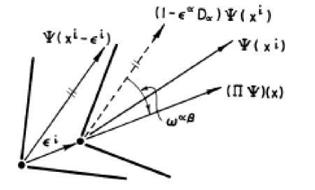
Figure 1: An infinitesimal active local Poincaré transformation of a matter field: The field $\psi(x^{i}-\varepsilon^{i})$ is first parallelly displaced over the infinitesimal vector $\varepsilon^{i}=e^{i}_{\hskip 0.6pt\cdot\hskip 1.2pt\gamma}\varepsilon^{\gamma}$, rotated by the angle $\omega^{\alpha\beta}$, and then compared with $\psi(x^{i})$.

The Lorentz-rotations (6 infinitesimal parameters $\omega^{\alpha\beta}$) are of the standard, special relativistic type. Hence the local P-transformation $\Pi$ of a field reads (see Figure 1):

$$(\Pi\psi)(x)=(1-\varepsilon^{\gamma}(x)D_{\gamma}+\omega^{\alpha\beta}(x)f_{\beta\alpha})\psi(x)\ .$$ (2.6)

Here again, the $f_{\beta\alpha}$ are the matrices of the Lorentz generators obeying (1.3). Of course, setting up a gauge theory, the $(4+6)$ infinitesimal “parameters” $(\varepsilon^{\gamma},\omega^{\alpha\beta})$ are spacetime dependent functions. A matter field distribution $\psi(x)$, such is our postulate, after the application of a local P-transformation $\Pi$, i.e. $\psi(x)\to(\Pi\psi)(x)$, is equivalent in all its measurable properties to the original distribution $\psi(x)$.

2.3 Commutation Relations, Torsion, and Curvature

The translation generators $D_{\gamma}$ and the rotation generators $f_{\beta\alpha}$ fulfill commutation relations which we will derive now. The commutation relations for the $f_{\beta\alpha}$ with themselves are given by the special relativistic formula (1.3). For rotations and translations we start with the relation $f_{\alpha\beta}D_{i}=D_{i}f_{\alpha\beta}$, which is valid since $D_{i}$ doesn’t carry a tetrad index. Let us remind ourselves that the $f_{\alpha\beta}$, as operators, act on everything to their rights. Transvecting with $e^{i}_{\hskip 0.6pt\cdot\hskip 1.2pt\gamma}$, we find $e^{i}_{\hskip 0.6pt\cdot\hskip 1.2pt\gamma}f_{\alpha\beta}D_{i}=D_{\gamma}f_{\alpha\beta}$, i.e.,

$$[f_{\alpha\beta},D_{\gamma}]=[f_{\alpha\beta},e^{i}_{\hskip 0.6pt\cdot\hskip 1.2pt\gamma}]D_{i}=\eta_{\gamma[\alpha}D_{\beta]}\ .$$ (2.7)

This formula is strictly analogous to its special relativistic pendant.

Finally, let us consider the translations under themselves. By explicit application of (2.5), we find

$$[D_{i},D_{j}]=F_{ij}^{\hskip 0.6pt\cdot\hskip 1.2pt\hskip 0.6pt\cdot\hskip 1.2pt\alpha\beta}f_{\beta\alpha}\ ,$$ (2.8)

where

$$F_{ij\alpha}^{\hskip 0.6pt\cdot\hskip 1.2pt\hskip 0.6pt\cdot\hskip 1.2pt\hskip 0.6pt\cdot\hskip 1.2pt\beta}:=2\bigg{(}\partial_{[i}\Gamma_{j]\alpha}^{\hskip 0.6pt\cdot\hskip 1.2pt\ \hskip 0.6pt\cdot\hskip 1.2pt\beta}+\Gamma_{[i|\gamma}^{\hskip 0.6pt\cdot\hskip 1.2pt\ \hskip 0.6pt\cdot\hskip 1.2pt\beta}\Gamma_{|j]\alpha}^{\,\hskip 0.6pt\cdot\hskip 1.2pt\ \hskip 0.6pt\cdot\hskip 1.2pt\gamma}\bigg{)}$$ (2.9)

is the curvature tensor (rotation field strength). Now $D_{i}=e_{i}^{\hskip 0.6pt\cdot\hskip 1.2pt\alpha}D_{\alpha}$, substitute it into (2.8) and define the torsion tensor (translation field strength),

$$F_{ij}^{\hskip 0.6pt\cdot\hskip 1.2pt\hskip 0.6pt\cdot\hskip 1.2pt\alpha}:=2D_{[i}e_{j]}^{\hskip 0.6pt\cdot\hskip 1.2pt\alpha}=2\bigg{(}\partial_{[i}e_{j]}^{\hskip 0.6pt\cdot\hskip 1.2pt\alpha}+\Gamma_{[i|\beta}^{\hskip 0.6pt\cdot\hskip 1.2pt\ \hskip 0.6pt\cdot\hskip 1.2pt\alpha}e_{|j]}^{\,\hskip 0.6pt\cdot\hskip 1.2pt\beta}\bigg{)}$$ (2.10)

Then finally, collecting all relevant commutation relations, we have

$$[D_{\alpha},D_{\beta}]=-F_{\alpha\beta}^{\hskip 0.6pt\cdot\hskip 1.2pt\hskip 0.6pt\cdot\hskip 1.2pt\gamma}D_{\gamma}+F_{\alpha\beta}^{\hskip 0.6pt\cdot\hskip 1.2pt\hskip 0.6pt\cdot\hskip 1.2pt\gamma\delta}f_{\delta\gamma}\ ,$$ (2.11)

$$[f_{\alpha\beta},D_{\gamma}]=\eta_{\gamma[\alpha}D_{\beta]}\ ,$$ (2.12)

$$[f_{\alpha\beta},f_{\gamma\delta}]=\eta_{\gamma[\alpha}f_{\beta]\delta}-\eta_{\delta[\alpha}f_{\beta]\gamma}\ .$$ (2.13)

For vanishing torsion and curvature we recover the commutation relations of global P-transformations. Local P-transformations, in contrast to the corresponding structures in gauge theories of internal symmetries, obey different commutation relations, in particular the algebra of the translations doesn’t close in general. Observe, however, that it does close for vanishing curvature, i.e. in a spacetime with teleparallelism (see Section 2.7). In introducing our translation generators, we already stressed their unique features. This is now manifest in (2.11). Note also that the “mixing term” $2\Gamma_{[i|\beta}^{\hskip 0.6pt\cdot\hskip 1.2pt\ \hskip 0.6pt\cdot\hskip 1.2pt\alpha}e_{|j]}^{\,\hskip 0.6pt\cdot\hskip 1.2pt\beta}$ between translational and rotational potentials in the’definition (2.10) of the translation field is due to the existence of orbital angular momentum.

In deriving (2.11), we find in torsion and curvature the tensors which covariantly characterize the possibly different arrangement of tetrads in comparison with that in special relativity. Torsion and curvature measure the non-minkowskian behavior of the tetrad arrangement. In (2.11) they relate to the translation and rotation generators, respectively. Consequently torsion represents the translation field strength and curvature the rotation field strength.

The only non-trivial Jacobi identity,

$$[D_{\alpha},[D_{\beta},D_{\gamma}]]+[D_{\beta},[D_{\gamma},D_{\alpha}]]+[D_{\gamma},[D_{\alpha},D_{\beta}]]=0\ ,$$ (2.14)

leads, after substitution of (2.11), some algebra and using (2.44), to the two sets of Bianchi identities

$$D_{[i}F_{jk]}^{\hskip 0.6pt\cdot\hskip 1.2pt\hskip 0.6pt\cdot\hskip 1.2pt\,\beta}\equiv F_{[ijk]}^{\hskip 0.6pt\cdot\hskip 1.2pt\hskip 0.6pt\cdot\hskip 1.2pt\hskip 0.6pt\cdot\hskip 1.2pt\,\beta}\ ,$$ (2.15)

$$D_{[i}F_{jk]\alpha}^{\hskip 0.6pt\cdot\hskip 1.2pt\hskip 0.6pt\cdot\hskip 1.2pt\,\hskip 0.6pt\cdot\hskip 1.2pt\beta}\equiv 0\ .$$ (2.16)

2.4 Local P-Transformation of the Gauge Potentials

Let us now come back to our postulate of local P-invariance. A matter field distribution actively P-transformed, $\psi(x)\to(\Pi\psi)(x)$ , should be equivalent to $\psi(x)$ . How can it happen that a local observer doesn’t see a difference in the field configuration after applying the P-transformation? The local P-transformation will induce not only a variation of $\psi(x)$ , but also correct the values of the tetrad coefficients $e_{i}^{\hskip 0.6pt\cdot\hskip 1.2pt\alpha}$ and the connection coefficients $\Gamma_{i}^{\hskip 0.6pt\cdot\hskip 1.2pt\alpha\beta}$ such that a difference doesn’t show up. In other words, the local P-transformation adjusts suitably the relative position and the relative orientation of the tetrads as determined by the corresponding coefficients ($e_{i}^{\hskip 0.6pt\cdot\hskip 1.2pt\alpha},\Gamma_{i}^{\hskip 0.6pt\cdot\hskip 1.2pt\alpha\beta}$). Thereby the P-transformation of the gauge potentials is a consequence of the local P-structure of spacetime.

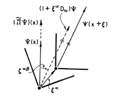
Figure 2: A matter field distribution near $x^{k}$.

Consider a matter field distribution $\psi(x)$, in particular its values at $x^{k}$ and at a nearby point $x^{k}+\xi^{k}$. See Figure 2 where the matter field is symbolized by a vector. The relative position of $\psi(x+\xi)$ and $\psi(x)$ is determined by $\xi^{\alpha}$, their relative orientation by $\zeta^{\alpha\beta}=\zeta^{[\alpha\beta]}$, the angle between $(1+\xi^{\alpha}D_{\alpha})\psi(x)$ and $\psi(x)$. By a rotation $-\zeta^{\alpha\beta}$ of $(1+\xi^{\alpha}D_{\alpha})\psi(x)$, we get $(\tilde{\Pi}\psi)(x)=(1+\xi^{\alpha}D_{\alpha}-\zeta^{\alpha\beta}f_{\beta\alpha})\times{\mathop{\psi}}(x)$, which is, of course, parallel to $\psi(x)$. The transformation $\tilde{\Pi}$ has the same structure as a P-transformation.

Now P-transform $\psi(x)$ and $\psi(x+\xi)$. Then $(\tilde{\Pi}\psi)(x)$ must stay parallel to $\psi(x)$, i.e. it is required to transform as a P-spinor-tensor. Furthermore $(\Pi\psi)(x+\xi)$ and $(\Pi\psi)(x)$, the P-transforms of the fields $\psi(x+\xi)$ and $\psi(x)$, can be again related by a transformation of the type $\tilde{\Pi}$, i.e. there emerge new $\xi^{\alpha}$ and $\zeta^{\alpha\beta}$ which are the P-transforms of the old ones.

Consequently, $D_{\alpha}\psi$ as well as $f_{\alpha\beta}\psi$ transform as P-spinor-tensors, i.e. if, according to (2.6) $\psi\to\Pi\psi$, then

$$D_{\alpha}\psi\to\Pi D_{\alpha}\psi\ ,$$ (2.17)

$$f_{\alpha\beta}\psi\to\Pi f_{\alpha\beta}\psi\ .$$ (2.18)

This implies, via the commutation relations (2.11), that torsion $F_{\alpha\beta}^{\hskip 0.6pt\cdot\hskip 1.2pt\hskip 0.6pt\cdot\hskip 1.2pt\gamma}$ and curvature $F_{\alpha\beta}^{\hskip 0.6pt\cdot\hskip 1.2pt\hskip 0.6pt\cdot\hskip 1.2pt\gamma\delta}$ are also P-tensors, an information which will turn out to be useful in constructing invariant gauge field Lagrangians.

Now we have

$$\Pi D_{\alpha}\psi=(D_{\alpha}+\delta D_{\alpha})(\psi+\delta\psi)=(D_{\alpha}+\delta D_{\alpha})\Pi\psi$$ (2.19)

and, because $\Pi$ deviates only infinitesimally from unity,

$$\delta D_{\alpha}=[\Pi,D_{\alpha}]\ .$$ (2.20)

Analogously we find

$$\delta f_{\alpha\beta}=[\Pi,f_{\alpha\beta}]\ .$$ (2.21)

Substitution of $\Pi$ from (2.6) into (2.20), (2.21) and using the commutation relations (2.11)-(2.13), yields, respectively,

$$\delta D_{\alpha} = -[\varepsilon^{\gamma}D_{\gamma},D_{\alpha}]+[\omega^{\gamma\delta}f_{\delta\gamma},D_{\alpha}]$$ (2.22)

$$= -\Big{(}-D_{\alpha}\varepsilon^{\gamma}+\omega_{\alpha}^{\hskip 0.6pt\cdot\hskip 1.2pt\gamma}-\varepsilon^{\delta}F_{\delta\alpha}^{\hskip 0.6pt\cdot\hskip 1.2pt\hskip 0.6pt\cdot\hskip 1.2pt\gamma}\Big{)}D_{\gamma}$$

$$+\Big{(}-D_{\alpha}\omega^{\hskip 0.6pt\cdot\hskip 1.2pt\gamma}_{\varepsilon}-\varepsilon^{\delta}F_{\delta\alpha\varepsilon}^{\hskip 0.6pt\cdot\hskip 1.2pt\hskip 0.6pt\cdot\hskip 1.2pt\hskip 0.6pt\cdot\hskip 1.2pt\gamma}\Big{)}f_{\gamma}^{\hskip 0.6pt\cdot\hskip 1.2pt\varepsilon}\ ,$$

$$\delta f_{\alpha\beta} = -[\varepsilon^{\gamma}D_{\gamma},f_{\alpha\beta}]+[\omega^{\gamma\delta}f_{\delta\gamma},f_{\alpha\beta}]=0\ .$$ (2.23)

The coordinates are kept fixed during the active P-transformation. Then, using (2.5) and (2.23), we get

$$\delta D_{i}=\delta\Big{(}\partial_{i}+\Gamma_{i}^{\hskip 0.6pt\cdot\hskip 1.2pt\alpha\beta}f_{\beta\alpha}\Big{)}=\Big{(}\delta\Gamma_{i}^{\hskip 0.6pt\cdot\hskip 1.2pt\alpha\beta}\Big{)}f_{\beta\alpha}$$ (2.24)

or

$$\delta D_{\alpha}=\delta\Big{(}e^{i}_{\hskip 0.6pt\cdot\hskip 1.2pt\alpha}D_{i}\Big{)}=\Big{(}\delta e^{i}_{\hskip 0.6pt\cdot\hskip 1.2pt\alpha}\Big{)}D_{i}+e^{i}_{\hskip 0.6pt\cdot\hskip 1.2pt\alpha}\Big{(}\delta\Gamma_{i}^{\hskip 0.6pt\cdot\hskip 1.2pt\alpha\beta}\Big{)}f_{\beta\alpha}\ .$$ (2.25)

A comparison with (2.22) and remembering $\delta(e^{i}_{\hskip 0.6pt\cdot\hskip 1.2pt\alpha}e_{j}^{\hskip 0.6pt\cdot\hskip 1.2pt\alpha})=0$, yields the desired relations

$$\delta e_{i}^{\hskip 0.6pt\cdot\hskip 1.2pt\alpha}=-D_{i}\varepsilon^{\alpha}+\omega_{\gamma}^{\hskip 0.6pt\cdot\hskip 1.2pt\alpha}e_{i}^{\hskip 0.6pt\cdot\hskip 1.2pt\gamma}-\varepsilon^{\gamma}F_{\gamma i}^{\hskip 0.6pt\cdot\hskip 1.2pt\hskip 0.6pt\cdot\hskip 1.2pt\alpha}\ ,$$ (2.26)

$$\delta\Gamma_{i}^{\hskip 0.6pt\cdot\hskip 1.2pt\alpha\beta}=-D_{i}\omega^{\alpha\beta}-\varepsilon^{\gamma}F_{\gamma i}^{\hskip 0.6pt\cdot\hskip 1.2pt\hskip 0.6pt\cdot\hskip 1.2pt\alpha\beta}\,.$$ (2.27)

From gauge theories on internal groups we are just not used to the non-local terms carrying the gauge field strengths; this is again an outflow of the specific behavior of the translations. Otherwise, the first terms on the right hand sides of (2.26), (2.27), namely $-D_{i}\varepsilon^{\alpha}$ and $-D_{i}\omega^{\alpha\beta}$, are standard. They express the nonhomogeneous transformation behavior of the potentials under local P-gauge transformations, respectively, and it is because of this fact that the names translation and rotation gauge potential are justified. The term $(\omega_{\gamma}^{\hskip 0.6pt\cdot\hskip 1.2pt\alpha}e_{i}^{\hskip 0.6pt\cdot\hskip 1.2pt\gamma})$ in (2.26) shows that the tetrad, the translation potential, behaves as a vector under rotations. This leads us to expect, as indeed will turn out to be true, that $e_{i}^{\hskip 0.6pt\cdot\hskip 1.2pt\alpha}$, in contrast to the rotation potential $\Gamma_{i}^{\hskip 0.6pt\cdot\hskip 1.2pt\alpha\beta}$, should carry intrinsic spin.

Having a $U_{4}$ with torsion and curvature we know that besides local P-invariance, we have additionally invariance under general coordinate transformations. In fact, this coordinate invariance is also a consequence of our formalism (see [1]). Starting with a $U_{4}$, one can alternatively develop a “gauge” formalism with coordinate invariance and local Lorentz invariance as applied to tetrads as ingredients. The only difference is, however, that with our procedure we recover in the limiting case of an $M_{4}$ exactly the well-known global P-transformations of special relativity (see eq. (2.60)) including the corresponding conservation laws (see eqs. (3.12), (3.13)), whereas otherwise the global gauge limit in this sense is lost: We have only to remember that in special relativity energy-momentum conservation is not a consequence of coordinate invariance, but rather of invariance under translations.

2.5 Closure of the Local P-Transformations

Having discussed so far how the matter field $\psi(x)$ and the gauge potentials $e^{\hskip 0.6pt\cdot\hskip 1.2pt\alpha}_{i}$ and $\Gamma_{i}^{\hskip 0.6pt\cdot\hskip 1.2pt\alpha\beta}$ transform under local P-transformations, we would now like to show once more the intrinsic naturality and usefulness of the local P-formalism developed so far. We shall compute the commutator of two successive P-transformations $[\stackrel{{\scriptstyle 2}}{{\Pi}},\stackrel{{\scriptstyle 1}}{{\Pi}}]$. We will find out that it yields a third local P-transformation $\stackrel{{\scriptstyle 3}}{{\Pi}}$, the infinitesimal parameters ($\stackrel{{\scriptstyle 3}}{{\varepsilon}}{}^{\alpha},\stackrel{{\scriptstyle 3}}{{\omega}}{}^{\alpha\beta}$) of which depend in a suitable way on the parameters ($\stackrel{{\scriptstyle 1}}{{\varepsilon}}{}^{\alpha},\stackrel{{\scriptstyle 1}}{{\omega}}{}^{\alpha\beta}$) and ($\stackrel{{\scriptstyle 2}}{{\varepsilon}}{}^{\alpha},\stackrel{{\scriptstyle 2}}{{\omega}}{}^{\alpha\beta}$) of the two transformations $\stackrel{{\scriptstyle 1}}{{\Pi}}$ and $\stackrel{{\scriptstyle 2}}{{\Pi}}$, respectively.

Take the connection as an example. We have

$$\stackrel{{\scriptstyle 1}}{{\Gamma}}{}^{\hskip 0.6pt\cdot\hskip 1.2pt\alpha\beta}_{i}:=\stackrel{{\scriptstyle 1}}{{\Pi}}\Gamma_{i}^{\hskip 0.6pt\cdot\hskip 1.2pt\alpha\beta}=\Gamma_{i}^{\hskip 0.6pt\cdot\hskip 1.2pt\alpha\beta}-D_{i}\stackrel{{\scriptstyle 1}}{{\omega}}{}^{\alpha\beta}-\stackrel{{\scriptstyle 1}}{{\varepsilon}}{}^{\gamma}e_{i}^{\hskip 0.6pt\cdot\hskip 1.2pt\delta}F_{\gamma\delta}^{\hskip 0.6pt\cdot\hskip 1.2pt\hskip 0.6pt\cdot\hskip 1.2pt\alpha\beta}\ .$$ (2.28)

In the last term we have purposely written the curvature in its totally anholonomic form. Then it is a P-tensor, as we saw in the last section. Applying now $\stackrel{{\scriptstyle 2}}{{\Pi}}$, we have to keep in mind that $\stackrel{{\scriptstyle 2}}{{\Pi}}$ acts with respect to the transformed tetrad coefficients $\stackrel{{\scriptstyle 1}}{{e}}{}^{\hskip 0.6pt\cdot\hskip 1.2pt\delta}_{i}:=\stackrel{{\scriptstyle 1}}{{\Pi}}e_{i}^{\hskip 0.6pt\cdot\hskip 1.2pt\delta}$ as well as with respect to the transformed connection coefficients $\stackrel{{\scriptstyle 1}}{{\Gamma}}{}_{i}^{\hskip 0.6pt\cdot\hskip 1.2pt\alpha\beta}$. Consequently we have

$$\stackrel{{\scriptstyle 2}}{{\Pi}}\stackrel{{\scriptstyle 1}}{{\Gamma}}{}^{\hskip 0.6pt\cdot\hskip 1.2pt\alpha\beta}_{i}=\stackrel{{\scriptstyle 2}}{{\Pi}}\stackrel{{\scriptstyle 1}}{{\Pi}}\Gamma{}^{\hskip 0.6pt\cdot\hskip 1.2pt\alpha\beta}_{i}=\stackrel{{\scriptstyle 1}}{{\Gamma}}{}^{\hskip 0.6pt\cdot\hskip 1.2pt\alpha\beta}_{i}-\stackrel{{\scriptstyle 1}}{{D}}_{i}\stackrel{{\scriptstyle 2}}{{\omega}}{}^{\alpha\beta}-\stackrel{{\scriptstyle 2}}{{\varepsilon}}{}^{\gamma}\stackrel{{\scriptstyle 1}}{{e}}{}^{\hskip 0.6pt\cdot\hskip 1.2pt\delta}_{i}\stackrel{{\scriptstyle 1}}{{F}}{}_{\gamma\delta}^{\hskip 0.6pt\cdot\hskip 1.2pt\hskip 0.6pt\cdot\hskip 1.2pt\alpha\beta}\ .$$ (2.29)

Now we will evaluate the different terms in (2.29). By differentiation and by use of (2.28) we find

$$\stackrel{{\scriptstyle 1}}{{D}}_{i}\stackrel{{\scriptstyle 2}}{{\omega}}{}^{\alpha\beta} = D_{i}\stackrel{{\scriptstyle 2}}{{\omega}}{}^{\alpha\beta}+2\Big{(}\stackrel{{\scriptstyle 1}}{{\delta}}\Gamma_{i\mu}^{\hskip 0.6pt\cdot\hskip 1.2pt\hskip 0.6pt\cdot\hskip 1.2pt[\alpha|}\Big{)}\stackrel{{\scriptstyle 2}}{{\omega}}{}^{\mu|\beta]}$$ (2.30)

$$= {D}_{i}\stackrel{{\scriptstyle 2}}{{\omega}}{}^{\alpha\beta}-2\Big{(}D_{i}\stackrel{{\scriptstyle 1}}{{\omega}}{}_{\mu}^{\hskip 0.6pt\cdot\hskip 1.2pt[\alpha|}\Big{)}\stackrel{{\scriptstyle 2}}{{\omega}}{}^{\mu|\beta]}$$

$$-2\stackrel{{\scriptstyle 1}}{{\varepsilon}}{}^{\gamma}F_{\gamma i\mu}^{\hskip 0.6pt\cdot\hskip 1.2pt\hskip 0.6pt\cdot\hskip 1.2pt\hskip 0.6pt\cdot\hskip 1.2pt[\alpha|}\stackrel{{\scriptstyle 2}}{{\omega}}{}^{\mu|\beta]}\,.$$

Let us turn to the last term in (2.29). If we apply (2.26), it reads in the appropriate order:

$$\stackrel{{\scriptstyle 2}}{{\varepsilon}}{}^{\gamma}\stackrel{{\scriptstyle 1}}{{e}}{}^{\hskip 0.6pt\cdot\hskip 1.2pt\delta}_{i}\stackrel{{\scriptstyle 1}}{{F}}{}_{\gamma\delta}^{\hskip 0.6pt\cdot\hskip 1.2pt\hskip 0.6pt\cdot\hskip 1.2pt\alpha\beta} = \stackrel{{\scriptstyle 2}}{{\varepsilon}}{}^{\gamma}e^{\hskip 0.6pt\cdot\hskip 1.2pt\delta}_{i}\stackrel{{\scriptstyle 1}}{{F}}{}_{\gamma\delta}^{\hskip 0.6pt\cdot\hskip 1.2pt\hskip 0.6pt\cdot\hskip 1.2pt\alpha\beta}+\stackrel{{\scriptstyle 2}}{{\varepsilon}}{}^{\gamma}\Big{(}\stackrel{{\scriptstyle 1}}{{\delta}}e^{\hskip 0.6pt\cdot\hskip 1.2pt\delta}_{i}\Big{)}{F}_{\gamma\delta}^{\hskip 0.6pt\cdot\hskip 1.2pt\hskip 0.6pt\cdot\hskip 1.2pt\alpha\beta}$$ (2.31)

$$= \stackrel{{\scriptstyle 2}}{{\varepsilon}}{}^{\gamma}e^{\hskip 0.6pt\cdot\hskip 1.2pt\delta}_{i}\stackrel{{\scriptstyle 1}}{{F}}{}_{\gamma\delta}^{\hskip 0.6pt\cdot\hskip 1.2pt\hskip 0.6pt\cdot\hskip 1.2pt\alpha\beta}+\stackrel{{\scriptstyle 2}}{{\varepsilon}}{}^{\gamma}$$

$$\Big{(}-D_{i}\stackrel{{\scriptstyle 1}}{{\varepsilon}}{}^{\delta}+\stackrel{{\scriptstyle 1}}{{\omega}}{}^{\hskip 0.6pt\cdot\hskip 1.2pt\delta}_{\nu}e^{\hskip 0.6pt\cdot\hskip 1.2pt\nu}_{i}-\stackrel{{\scriptstyle 1}}{{\varepsilon}}{}^{\nu}{F}_{\nu i}^{\hskip 0.6pt\cdot\hskip 1.2pt\hskip 0.6pt\cdot\hskip 1.2pt\delta}\Big{)}{F}_{\gamma\delta}^{\hskip 0.6pt\cdot\hskip 1.2pt\hskip 0.6pt\cdot\hskip 1.2pt\alpha\beta}\ .$$

In (2.31) there occurs the P-transform of the anholonomic curvature. Like any P-tensor, it transforms according to (2.6):

$$\stackrel{{\scriptstyle 1}}{{F}}{}_{\gamma\delta}^{\hskip 0.6pt\cdot\hskip 1.2pt\hskip 0.6pt\cdot\hskip 1.2pt\alpha\beta}=F_{\gamma\delta}^{\hskip 0.6pt\cdot\hskip 1.2pt\hskip 0.6pt\cdot\hskip 1.2pt\alpha\beta}-\stackrel{{\scriptstyle 1}}{{\varepsilon}}{}^{\mu}D_{\mu}F_{\gamma\delta}^{\hskip 0.6pt\cdot\hskip 1.2pt\hskip 0.6pt\cdot\hskip 1.2pt\alpha\beta}-2\stackrel{{\scriptstyle 1}}{{\omega}}{}_{[\gamma|}^{\ \hskip 0.6pt\cdot\hskip 1.2pt\ \mu}F_{\mu|\delta]}^{\hskip 0.6pt\cdot\hskip 1.2pt\,\hskip 0.6pt\cdot\hskip 1.2pt\,\alpha\beta}+2\stackrel{{\scriptstyle 1}}{{\omega}}{}_{\mu}^{\hskip 0.6pt\cdot\hskip 1.2pt[\alpha|}F_{\gamma\delta}^{\hskip 0.6pt\cdot\hskip 1.2pt\hskip 0.6pt\cdot\hskip 1.2pt\mu|\beta]}\ .$$ (2.32)

Now we substitute first (2.32) into (2.31). The resulting equation together with (2.28) and (2.30) are then substituted into (2.29). After some reordering we find

$$\stackrel{{\scriptstyle 2}}{{\Pi}}\stackrel{{\scriptstyle 1}}{{\Pi}}\Gamma_{i}^{\hskip 0.6pt\cdot\hskip 1.2pt\alpha\beta} = \Gamma_{i}^{\hskip 0.6pt\cdot\hskip 1.2pt\alpha\beta}-D_{i}\Big{(}\stackrel{{\scriptstyle 1}}{{\omega}}{}^{\alpha\beta}+\stackrel{{\scriptstyle 2}}{{\omega}}{}^{\alpha\beta}\Big{)}-F_{\gamma i}^{\hskip 0.6pt\cdot\hskip 1.2pt\hskip 0.6pt\cdot\hskip 1.2pt\alpha\beta}\Big{(}\stackrel{{\scriptstyle 1}}{{\varepsilon}}{}^{\gamma}+\stackrel{{\scriptstyle 2}}{{\varepsilon}}{}^{\gamma}\Big{)}+$$ (2.33)

$$+F_{\gamma\delta}^{\hskip 0.6pt\cdot\hskip 1.2pt\hskip 0.6pt\cdot\hskip 1.2pt\alpha\beta}F_{\nu i}^{\hskip 0.6pt\cdot\hskip 1.2pt\hskip 0.6pt\cdot\hskip 1.2pt\delta}\stackrel{{\scriptstyle 1}}{{\varepsilon}}{}^{\nu}\stackrel{{\scriptstyle 2}}{{\varepsilon}}{}^{\gamma}+2D_{i}\Big{(}\stackrel{{\scriptstyle 1}}{{\omega}}{}_{\mu}^{\hskip 0.6pt\cdot\hskip 1.2pt[\alpha|}\Big{)}\stackrel{{\scriptstyle 2}}{{\omega}}{}^{\mu|\beta]}+$$

$$+2F_{\gamma i\mu}^{\hskip 0.6pt\cdot\hskip 1.2pt\hskip 0.6pt\cdot\hskip 1.2pt\hskip 0.6pt\cdot\hskip 1.2pt[\alpha|}\Big{(}\stackrel{{\scriptstyle 1}}{{\varepsilon}}{}^{\gamma}\stackrel{{\scriptstyle 2}}{{\omega}}{}^{\mu|\beta]}+\stackrel{{\scriptstyle 2}}{{\varepsilon}}{}^{\gamma}\stackrel{{\scriptstyle 1}}{{\omega}}{}^{\mu|\beta]}\Big{)}+e^{\hskip 0.6pt\cdot\hskip 1.2pt\delta}_{i}F_{\mu\delta}^{\hskip 0.6pt\cdot\hskip 1.2pt\hskip 0.6pt\cdot\hskip 1.2pt\alpha\beta}\stackrel{{\scriptstyle 2}}{{\varepsilon}}{}^{\gamma}\omega_{\gamma}^{\hskip 0.6pt\cdot\hskip 1.2pt\mu}+$$

$$+e^{\hskip 0.6pt\cdot\hskip 1.2pt\delta}_{i}\Big{(}D_{\mu}F_{\gamma\delta}^{\hskip 0.6pt\cdot\hskip 1.2pt\hskip 0.6pt\cdot\hskip 1.2pt\alpha\beta}\Big{)}\stackrel{{\scriptstyle 2}}{{\varepsilon}}{}^{\gamma}\stackrel{{\scriptstyle 1}}{{\varepsilon}}{}^{\mu}+F_{\gamma\delta}^{\hskip 0.6pt\cdot\hskip 1.2pt\hskip 0.6pt\cdot\hskip 1.2pt\alpha\beta}\stackrel{{\scriptstyle 2}}{{\varepsilon}}{}^{\gamma}D_{i}\stackrel{{\scriptstyle 1}}{{\varepsilon}}{}^{\delta}\ .$$

I am not happy myself with all those indices. Anybody is invited to look for a simpler proof. But the main thing is done. The right-hand-side of (2.33) depends only on the untransformed geometrical quantities and on the parameters. By exchanging the one’s and two’s wherever they appear, we get the reversed order of the transformations:

$$\stackrel{{\scriptstyle 1}}{{\Pi}}\stackrel{{\scriptstyle 2}}{{\Pi}}\Gamma_{i}^{\hskip 0.6pt\cdot\hskip 1.2pt\alpha\beta}=(\ref{233})\quad\textrm{with}\quad\begin{array}[]{rl}1\to 2\\ 2\to 1\end{array}\ .$$ (2.34)

Subtracting (2.34) from (2.33) yields the commutator $[\stackrel{{\scriptstyle 2}}{{\Pi}}\stackrel{{\scriptstyle 1}}{{\Pi}}]\Gamma_{i}^{\hskip 0.6pt\cdot\hskip 1.2pt\alpha\beta}$.

After some heavy algebra and application of the 2nd Bianchi identity in its anholonomic form,

$$D_{[\alpha}F_{\beta\gamma]}^{\hskip 0.6pt\cdot\hskip 1.2pt\hskip 0.6pt\cdot\hskip 1.2pt\mu\nu}=F_{[\alpha\beta}^{\hskip 0.6pt\cdot\hskip 1.2pt\,\hskip 0.6pt\cdot\hskip 1.2pt\delta}F_{\gamma]\delta}^{\hskip 0.6pt\cdot\hskip 1.2pt\,\hskip 0.6pt\cdot\hskip 1.2pt\mu\nu}\ ,$$ (2.35)

we find indeed a transformation $\stackrel{{\scriptstyle 3}}{{\Pi}}\Gamma_{i}^{\hskip 0.6pt\cdot\hskip 1.2pt\alpha\beta}$ of the form (2.28) with the following parameters:

$$\stackrel{{\scriptstyle 3}}{{\varepsilon}}{}^{\alpha}=-\stackrel{{\scriptstyle 2}}{{\omega}}{}^{\hskip 0.6pt\cdot\hskip 1.2pt\alpha}_{\gamma}\stackrel{{\scriptstyle 1}}{{\varepsilon}}{}^{\gamma}+\stackrel{{\scriptstyle 1}}{{\omega}}{}^{\hskip 0.6pt\cdot\hskip 1.2pt\alpha}_{\gamma}\stackrel{{\scriptstyle 2}}{{\varepsilon}}{}^{\gamma}-\stackrel{{\scriptstyle 2}}{{\varepsilon}}{}^{\beta}\stackrel{{\scriptstyle 1}}{{\varepsilon}}{}^{\gamma}F_{\beta\gamma}^{\hskip 0.6pt\cdot\hskip 1.2pt\hskip 0.6pt\cdot\hskip 1.2pt\alpha}\ ,$$ (2.36)

$$\stackrel{{\scriptstyle 3}}{{\omega}}{}^{\hskip 0.6pt\cdot\hskip 1.2pt\beta}_{\alpha}=-\stackrel{{\scriptstyle 2}}{{\omega}}{}^{\hskip 0.6pt\cdot\hskip 1.2pt\gamma}_{\alpha}\stackrel{{\scriptstyle 1}}{{\omega}}{}^{\hskip 0.6pt\cdot\hskip 1.2pt\beta}_{\gamma}+\stackrel{{\scriptstyle 1}}{{\omega}}{}^{\hskip 0.6pt\cdot\hskip 1.2pt\gamma}_{\alpha}\stackrel{{\scriptstyle 2}}{{\omega}}{}^{\hskip 0.6pt\cdot\hskip 1.2pt\beta}_{\gamma}-\stackrel{{\scriptstyle 2}}{{\varepsilon}}{}^{\gamma}\stackrel{{\scriptstyle 1}}{{\varepsilon}}{}^{\delta}F_{\gamma\delta\alpha}^{\hskip 0.6pt\cdot\hskip 1.2pt\hskip 0.6pt\cdot\hskip 1.2pt\beta}\ .$$ (2.37)

It is straightforward to show that the corresponding formulae for $[\stackrel{{\scriptstyle 2}}{{\Pi}}\stackrel{{\scriptstyle 1}}{{\Pi}}]$ as a applied to the matter field and the tetrad lead to the same parameters (2.36), (2.37). These results are natural generalizations of the corresponding commutator in an $M_{4}$. One can take (2.36), (2.37) as the ultimate justification for attributing a fundamental significance to the notion of a local P-transformation.

2.6 Local Kinematical Inertial Frames

As we have seen in (1.8) , (1.9), in an $M_{4}$ we can always trivialize the gauge potentials globally. Since spacetime looks minkowskian from a local point of view, it should be possible to trivialize the gauge potentials in a $U_{4}$ locally, i.e.,

$$\left\{\begin{array}[]{rl}e_{i}^{\hskip 0.6pt\cdot\hskip 1.2pt\alpha}\big{(}x^{k}=\mathop{x}\limits_{0}\,^{k}\big{)}\stackrel{{\scriptstyle\star}}{{=}}\delta^{\alpha}_{i}\ ,\\[9.0pt] \Gamma_{i}^{\hskip 0.6pt\cdot\hskip 1.2pt\alpha\beta}\big{(}x^{k}=\mathop{x}\limits_{0}\,^{k}\big{)}\stackrel{{\scriptstyle\star}}{{=}}0.\end{array}\right\}$$ (2.38)

The proof runs as follows: We rotate the tetrads according to ${e^{\prime}}^{\hskip 0.6pt\cdot\hskip 1.2pt\alpha}_{i}=\Lambda_{\beta}^{\hskip 0.6pt\cdot\hskip 1.2pt\alpha}e_{i}^{\hskip 0.6pt\cdot\hskip 1.2pt\beta}$. This induces a transformation of the connection, namely the finite version of (2.27) for $\varepsilon^{\gamma}=0$:

$${\Gamma^{\prime}}_{i\alpha}^{\hskip 0.6pt\cdot\hskip 1.2pt\hskip 0.6pt\cdot\hskip 1.2pt\beta}=\Lambda_{\alpha}^{\hskip 0.6pt\cdot\hskip 1.2pt\gamma}\Lambda_{\delta}^{\hskip 0.6pt\cdot\hskip 1.2pt\beta}\Gamma_{i\gamma}^{\hskip 0.6pt\cdot\hskip 1.2pt\hskip 0.6pt\cdot\hskip 1.2pt\delta}-\Lambda_{\alpha}^{\hskip 0.6pt\cdot\hskip 1.2pt\gamma}\partial_{i}\Lambda_{\gamma}^{\hskip 0.6pt\cdot\hskip 1.2pt\beta}\ .$$ (2.39)

By a suitable choice of the rotation, we want these transformed connection coefficients to vanish. We put (2.39) provisionally equal to zero, solve for $\partial_{i}\Lambda_{\beta}^{\hskip 0.6pt\cdot\hskip 1.2pt\alpha}$, and find

$$\partial_{i}\Lambda_{\beta}^{\hskip 0.6pt\cdot\hskip 1.2pt\alpha}=\Lambda_{\gamma}^{\hskip 0.6pt\cdot\hskip 1.2pt\alpha}\Gamma_{i\beta}^{\hskip 0.6pt\cdot\hskip 1.2pt\hskip 0.6pt\cdot\hskip 1.2pt\gamma}\Big{(}x^{k}=\mathop{x}\limits_{0}\,^{k}\Big{)}\ .$$ (2.40)

For prescribed $\Gamma_{i\beta}^{\hskip 0.6pt\cdot\hskip 1.2pt\hskip 0.6pt\cdot\hskip 1.2pt\gamma}$ at $x^{k}=\mathop{x}\limits_{0}\,^{k}$ we can always solve this first order linear differential equation, which concludes the first part of the proof. Then we adjust the holonomic coordinates. The connection $\Gamma_{i}^{\hskip 0.6pt\cdot\hskip 1.2pt\alpha\beta}\stackrel{{\scriptstyle\star}}{{=}}0$, being a coordinate vector, stays zero, whereas the tetrad transforms as follows: ${e^{\prime}}^{\hskip 0.6pt\cdot\hskip 1.2pt\alpha}_{i}=(\partial x^{k}/\partial{x^{\prime}}^{i})e_{k}^{\hskip 0.6pt\cdot\hskip 1.2pt\alpha}$. For a transformation of the type ${x^{\prime}}^{i}=\delta^{i}_{\beta}e_{\ell}^{\hskip 0.6pt\cdot\hskip 1.2pt\beta}x^{\ell}$+ const. we find indeed ${e^{\prime}}^{\hskip 0.6pt\cdot\hskip 1.2pt\alpha}_{i}\stackrel{{\scriptstyle\star}}{{=}}\delta_{i}^{\alpha}$, q.e.d.

What is the physical meaning of these trivial gauge frames existing all over spacetime? Evidently they represent in a Riemann-Cartan spacetime what was in Einstein’s theory the freely falling non-rotating elevator. For these considerations it is vital, however, that from our gauge theoretical point of view the potentials $(e_{i}^{\hskip 0.6pt\cdot\hskip 1.2pt\alpha},\Gamma_{i}^{\hskip 0.6pt\cdot\hskip 1.2pt\alpha\beta})$ are locally measurable, whereas torsion and curvature, as derivatives of the potentials, are only to be measured in a nonlocal way. For a local observer the world looks minkowskian. If he wants to determine, e.g., whether his world embodies torsion, he has to communicate with his neighbors thereby implying nonlocality. This example shows that in the PG the question whether spacetime carries torsion or not (or curvature or not) is not a question one should ask one local observer.

It is to be expected that non-local quantities like torsion and curvature, in analogy to Maxwell’s theory and GR, are governed by field equations. In other words, whether, for instance, the world is riemannian or not, should in the framework of the PG not be imposed ad hoc but rather left as a question to dynamics.

We call the frames (2.38) “local kinematical inertial frames” in order to distinguish them from the local “dynamical” inertial frames in Einstein’s GR. In the PG the notion of inertia refers to translation and rotation, or to mass and spin. A coordinate frame $\boldsymbol{\partial}_{i}$ of GR has to fulfill the differential constraint $\Omega_{ij}^{\hskip 0.6pt\cdot\hskip 1.2pt\hskip 0.6pt\cdot\hskip 1.2pt\alpha}(\boldsymbol{\partial})\equiv 0$, see eq. (1.5). Hence a tetrad frame, which is unconstrained, can move more freely and is, as compared to the coordinate frame, a more local object. Accordingly, the notion of inertia in the PG is more local than that in GR. This is no surprise, since a test particle of GR carries a mass $m$ which is a quantity won by integration over an extended energy-momentum distribution. The matter field $\psi(x)$, however, the object of consideration in the PG, is clearly a more localized being.

A natural extension of the Einstein equivalence principle to the PG would then be to postulate that in the frames (2.38) (these are our new “elevators”) special relativity is valid locally. Consequently the special-relativistic matter lagrangian $L$ in (1.10) should in a $U_{4}$ be a lagrangian density ${\cal L}$ which couples to spacetime according to

$${\cal L}={\cal L}\Big{(}\psi,\partial_{i}\psi,e_{i}^{\hskip 0.6pt\cdot\hskip 1.2pt\alpha},\Gamma_{i}^{\hskip 0.6pt\cdot\hskip 1.2pt\alpha\beta}\Big{)}\stackrel{{\scriptstyle\star}}{{=}}L(\psi,\partial_{i}\psi)\ ,$$ (2.41)

i.e. in the local kinematical inertial frames everything looks special relativistic. Observe that derivatives of $(e_{i}^{\hskip 0.6pt\cdot\hskip 1.2pt\alpha},\Gamma_{i}^{\hskip 0.6pt\cdot\hskip 1.2pt\alpha\beta})$ are excluded by our “local equivalence principle”. Strictly this discussion belongs into Lecture 3. But the geometry is so suggestive to physical applications that we cannot resist the temptation to present the local equivalence principle already in the context of spacetime geometry.

Naturally, as argued above, the local equivalence principle is not to be applied to directly observable objects like mass points, but rather to the more abstract notion of a lagrangian. In a field theory there seems to be no other reasonable option. And we have seen that the fermionic nature of the building blocks of matter require a field description, at least on a $c$-number level. Accordingly (2.41) appears to be the natural extension of Einstein’s equivalence principle to the PG.

2.7 Riemann-Cartan Spacetime Seen Anholonomically and Holonomically

We have started our geometrical game with the $(e_{i}^{\hskip 0.6pt\cdot\hskip 1.2pt\alpha},\Gamma_{i}^{\hskip 0.6pt\cdot\hskip 1.2pt\alpha\beta})$-set. We would now like to provide some machinery for translating this anholonomic formalism into the holonomic formalism commonly more known at least under relativists. Let us first collect some useful formulae for the anholonomic regime. The determinant $e:=\textrm{det}\,e_{i}^{\hskip 0.6pt\cdot\hskip 1.2pt\alpha}$ is a scalar density, furthermore, by some algebra we get $D_{i}e=\partial_{i}e$. If we apply the Leibniz rule the definitions (2.5) and (2.10), we find successively $(F_{\alpha}:=F_{\alpha\gamma}^{\hskip 0.6pt\cdot\hskip 1.2pt\hskip 0.6pt\cdot\hskip 1.2pt\gamma})$

$$D_{i}(ee^{i}_{\hskip 0.6pt\cdot\hskip 1.2pt\alpha})=eF_{\alpha}\ ,$$ (2.42)

$$2D_{j}\Big{(}ee^{i}_{\hskip 0.6pt\cdot\hskip 1.2pt[\alpha}e^{j}_{\hskip 0.6pt\cdot\hskip 1.2pt\beta]}\Big{)}=e\Big{(}F_{\alpha\beta}^{\hskip 0.6pt\cdot\hskip 1.2pt\hskip 0.6pt\cdot\hskip 1.2pti}+2e^{i}_{\hskip 0.6pt\cdot\hskip 1.2pt[\alpha}F_{\beta]}\Big{)}\ ,$$ (2.43)

$$D_{[\alpha}(e^{i}_{\hskip 0.6pt\cdot\hskip 1.2pt\beta}e^{j}_{\hskip 0.6pt\cdot\hskip 1.2pt\gamma]})=e^{[i}_{\,\hskip 0.6pt\cdot\hskip 1.2pt[\alpha}F^{\hskip 0.6pt\cdot\hskip 1.2pt\hskip 0.6pt\cdot\hskip 1.2pt\ j]}_{\beta\gamma]}\ .$$ (2.44)

The last formula was convenient for rewriting the 2nd Bianchi identity (2.16), which was first given in a completely anholonomic form. Eq. (2.43), defining the “modified torsion tensor” on its right hand side, will be used in the context of the field equations to be derived in Section 4.4.

Now, according to (2.1), $dx^{i}\Gamma_{i}^{\hskip 0.6pt\cdot\hskip 1.2pt\alpha\beta}\mbox{\boldmath$e$}_{\beta}$ is the relative rotation encountered by a tetrad $\mbox{\boldmath$e$}_{\alpha}$ in going from $x^{k}$ to $x^{k}+dx^{k}$. From this we can calculate that the relative rotation of the respective coordinate frame $\boldsymbol{\partial}_{j}=e_{j}^{\hskip 0.6pt\cdot\hskip 1.2pt\alpha}\mbox{\boldmath$e$}_{\alpha}$ is $dx^{i}(\Gamma_{i\beta}^{\hskip 0.6pt\cdot\hskip 1.2pt\hskip 0.6pt\cdot\hskip 1.2pt\alpha}e_{j}^{\hskip 0.6pt\cdot\hskip 1.2pt\beta}+\partial_{i}e_{j}^{\hskip 0.6pt\cdot\hskip 1.2pt\alpha})\mbox{\boldmath$e$}_{\alpha}$. In a holonomic coordinate system, the parallel transport is thus given by

$$\nabla_{i}:=\partial_{i}+\tilde{\Gamma}_{ij}^{\hskip 0.6pt\cdot\hskip 1.2pt\hskip 0.6pt\cdot\hskip 1.2ptk}h_{k}^{\hskip 0.6pt\cdot\hskip 1.2ptj}\ ,$$ (2.45)

where $h$ represents the generator of coordinate transformation for tensors fields and

$$\tilde{\Gamma}_{ij}^{\hskip 0.6pt\cdot\hskip 1.2pt\hskip 0.6pt\cdot\hskip 1.2ptk}:=e_{j}^{\hskip 0.6pt\cdot\hskip 1.2pt\alpha}e^{k}_{\hskip 0.6pt\cdot\hskip 1.2pt\beta}\Gamma_{i\alpha}^{\hskip 0.6pt\cdot\hskip 1.2pt\hskip 0.6pt\cdot\hskip 1.2pt\beta}+e^{k}_{\hskip 0.6pt\cdot\hskip 1.2pt\beta}\partial_{i}e^{\hskip 0.6pt\cdot\hskip 1.2pt\beta}_{j}\ .$$ (2.46)

This relation translates the anholonomic into the holonomic connection. Observe that for a connection the conversion of holonomic to anholonomic indices and vice versa is markedly different from the simple transvection rule as applied to tensors. The holonomic components of the covariant derivative of a tensor $A$ are given with respect to its anholonomic components by

$$\nabla_{i}A_{j\hskip 0.6pt\cdot\hskip 1.2pt\hskip 0.6pt\cdot\hskip 1.2pt}^{\ \ \ \ k\hskip 0.6pt\cdot\hskip 1.2pt\hskip 0.6pt\cdot\hskip 1.2pt}=e_{j}^{\hskip 0.6pt\cdot\hskip 1.2pt\alpha}\hskip 0.6pt\cdot\hskip 1.2pt\hskip 0.6pt\cdot\hskip 1.2pt\ e^{k}_{\hskip 0.6pt\cdot\hskip 1.2pt\beta}\hskip 0.6pt\cdot\hskip 1.2pt\hskip 0.6pt\cdot\hskip 1.2pt\ D_{i}A_{\alpha\hskip 0.6pt\cdot\hskip 1.2pt\hskip 0.6pt\cdot\hskip 1.2pt}^{\ \ \ \ \beta\hskip 0.6pt\cdot\hskip 1.2pt\hskip 0.6pt\cdot\hskip 1.2pt}\ .$$ (2.47)

The concept of parallelism with respect to a coordinate frame, as defined in (2.46), is by construction locally identical with minkowskian parallelism, as is measured in a local tetrad. In a similar way, the local minkowskian length and angle measurements define the metric in a coordinate frame:

$$g_{ij}(x^{k}):=e_{i}^{\hskip 0.6pt\cdot\hskip 1.2pt\alpha}(x^{k})e_{j}^{\hskip 0.6pt\cdot\hskip 1.2pt\beta}(x^{k})\eta_{\alpha\beta}\ .$$ (2.48)

From the antisymmetry $\Gamma_{i}^{\hskip 0.6pt\cdot\hskip 1.2pt\alpha\beta}=-\Gamma_{i}^{\hskip 0.6pt\cdot\hskip 1.2pt\beta\alpha}$ of the anholonomic connection and from (2.47) results again $D_{i}\eta_{\alpha\beta}=0$, a relation which we used already earlier, and

$$\nabla_{i}g_{jk}=0\ ,$$ (2.49)

the so-called metric postulate of spacetime physics.

If we resolve (2.49) with respect to $\tilde{\Gamma}_{ij}^{\hskip 0.6pt\cdot\hskip 1.2pt\hskip 0.6pt\cdot\hskip 1.2ptk}$, we get

$$\tilde{\Gamma}_{ij}^{\hskip 0.6pt\cdot\hskip 1.2pt\hskip 0.6pt\cdot\hskip 1.2ptk}=\left\{\begin{array}[]{rl}k\\ ij\end{array}\right\}+\frac{1}{2}F_{ij}^{\hskip 0.6pt\cdot\hskip 1.2pt\hskip 0.6pt\cdot\hskip 1.2ptk}-\frac{1}{2}F_{j\hskip 0.6pt\cdot\hskip 1.2pti}^{\hskip 0.6pt\cdot\hskip 1.2ptk}+\frac{1}{2}F^{k}_{\hskip 0.6pt\cdot\hskip 1.2ptij}$$ (2.50)

and, taking (2.46) into account, the corresponding relation for the anholonomic connection:

$$\Gamma_{\alpha\beta\gamma}:=e^{i}_{\hskip 0.6pt\cdot\hskip 1.2pt\alpha}\Gamma_{i\beta\gamma}=(-\Omega_{\alpha\beta\gamma}+\Omega_{\beta\gamma\alpha}-\Omega_{\gamma\alpha\beta}+F_{\alpha\beta\gamma}-F_{\beta\gamma\alpha}+F_{\gamma\alpha\beta})/2\ .$$ (2.51)

We have introduced here the Christoffel symbol $\left\{\begin{array}[]{rl}k\\ ij\end{array}\right\}$, the holonomic components of the torsion tensor,

$$F_{ij}^{\hskip 0.6pt\cdot\hskip 1.2pt\hskip 0.6pt\cdot\hskip 1.2ptk}=e^{k}_{\hskip 0.6pt\cdot\hskip 1.2pt\alpha}F_{ij}^{\hskip 0.6pt\cdot\hskip 1.2pt\hskip 0.6pt\cdot\hskip 1.2pt\alpha}=2\tilde{\Gamma}_{[ij]}^{\,\hskip 0.6pt\cdot\hskip 1.2pt\hskip 0.6pt\cdot\hskip 1.2pt\,k}\ ,$$ (2.52)

and the object of anholonomity

$$\Omega_{\alpha\beta}^{\hskip 0.6pt\cdot\hskip 1.2pt\hskip 0.6pt\cdot\hskip 1.2pt\gamma}:=e^{i}_{\hskip 0.6pt\cdot\hskip 1.2pt\alpha}e^{j}_{\hskip 0.6pt\cdot\hskip 1.2pt\beta}\Omega_{ij}^{\hskip 0.6pt\cdot\hskip 1.2pt\hskip 0.6pt\cdot\hskip 1.2pt\gamma}\ ;\quad\Omega_{ij}^{\hskip 0.6pt\cdot\hskip 1.2pt\hskip 0.6pt\cdot\hskip 1.2pt\gamma}:=2\partial_{[i}e_{j]}^{\hskip 0.6pt\cdot\hskip 1.2pt\,\gamma}\ .$$ (2.53)

Expressing the holonomic components of the curvature tensor in terms of $\tilde{\Gamma}_{ij}^{\hskip 0.6pt\cdot\hskip 1.2pt\hskip 0.6pt\cdot\hskip 1.2ptk}$ yields

$$F_{ij\,k}^{\hskip 0.6pt\cdot\hskip 1.2pt\hskip 0.6pt\cdot\hskip 1.2pt\hskip 0.6pt\cdot\hskip 1.2pt\ell}=2\Big{(}\partial_{[i}\tilde{\Gamma}_{j]k}^{\hskip 0.6pt\cdot\hskip 1.2pt\,\hskip 0.6pt\cdot\hskip 1.2pt\ell}+\tilde{\Gamma}_{[i|m}^{\,\hskip 0.6pt\cdot\hskip 1.2pt\,\hskip 0.6pt\cdot\hskip 1.2pt\ell}\tilde{\Gamma}_{|j]k}^{\,\hskip 0.6pt\cdot\hskip 1.2pt\,\hskip 0.6pt\cdot\hskip 1.2ptm}\Big{)}\ .$$ (2.54)

Finally, taking the antisymmetric part of (2.46) or using the definition of torsion (2.10), we get

$$F_{ij}^{\hskip 0.6pt\cdot\hskip 1.2pt\hskip 0.6pt\cdot\hskip 1.2pt\alpha}=\Omega_{ij}^{\hskip 0.6pt\cdot\hskip 1.2pt\hskip 0.6pt\cdot\hskip 1.2pt\alpha}-2e_{[i}^{\,\hskip 0.6pt\cdot\hskip 1.2pt\beta}\Gamma_{j]\beta}^{\hskip 0.6pt\cdot\hskip 1.2pt\,\hskip 0.6pt\cdot\hskip 1.2pt\alpha}\ ,$$ (2.55)

a formula which will play a key role in discussing macroscopic gravity: the object of anholonomity mediates between torsion and the anholonomic connection.

Eq. (2.50) shows that instead of the potentials $(e_{i}^{\hskip 0.6pt\cdot\hskip 1.2pt\alpha},\Gamma_{i}^{\hskip 0.6pt\cdot\hskip 1.2pt\alpha\beta})$ we can use holonomically the set $(g_{ij},S_{ij}^{\hskip 0.6pt\cdot\hskip 1.2pt\hskip 0.6pt\cdot\hskip 1.2ptk})$, the geometry is always a Riemann-Cartan one, only the mode of description is different. In the holonomic description $e_{i}^{\hskip 0.6pt\cdot\hskip 1.2pt\alpha}$ enters the definition of torsion $F_{ij}^{\hskip 0.6pt\cdot\hskip 1.2pt\hskip 0.6pt\cdot\hskip 1.2pt\alpha}$, hence we should not use $F_{ij}^{\hskip 0.6pt\cdot\hskip 1.2pt\hskip 0.6pt\cdot\hskip 1.2pt\alpha}$ as an independent variable in place of $\Gamma_{i}^{\hskip 0.6pt\cdot\hskip 1.2pt\alpha\beta}$. The anholonomic formalism is superior in a gauge approach, because $(e_{i}^{\hskip 0.6pt\cdot\hskip 1.2pt\alpha},\Gamma_{i}^{\hskip 0.6pt\cdot\hskip 1.2pt\alpha\beta})$ are supposed to be directly measurable and have an interpretation as potentials and the corresponding transformation behavior, whereas the holonomic set $(g_{ij},S_{ij}^{\hskip 0.6pt\cdot\hskip 1.2pt\hskip 0.6pt\cdot\hskip 1.2ptk})$ is a tensorial one.

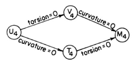
Figure 3: The Riemann-Cartan spacetime $U_{4}$ and its limiting cases:
$T_{4}$ = teleparallelism, $V_{4}$ = Riemann, $M_{4}$ = Minkowski.

If we put curvature to zero, we get a spacetime with teleparallelism $T_{4}$, a $U_{4}$ for vanishing torsion is a Riemann spacetime $V_{4}$, see Figure 3.

Perhaps surprisingly, as regards to their physical degrees of freedom, the $T_{4}$ and the $V_{4}$ are in some sense similar to each other. In a $T_{4}$ the curvature vanishes, i.e. the parallel transfer is integrable. Then we can always pick preferred tetrad frames such that the connection vanishes globally:

$$T_{4}:\ =\Big{(}e_{i}^{\hskip 0.6pt\cdot\hskip 1.2pt\alpha},\Gamma_{i}^{\hskip 0.6pt\cdot\hskip 1.2pt\alpha\beta}\stackrel{{\scriptstyle\star}}{{=}}0\Big{)}\ ;\quad\Big{(}F_{ij}^{\hskip 0.6pt\cdot\hskip 1.2pt\hskip 0.6pt\cdot\hskip 1.2pt\alpha}\stackrel{{\scriptstyle\star}}{{=}}\Omega_{ij}^{\hskip 0.6pt\cdot\hskip 1.2pt\hskip 0.6pt\cdot\hskip 1.2pt\alpha},F_{ij}^{\hskip 0.6pt\cdot\hskip 1.2pt\hskip 0.6pt\cdot\hskip 1.2pt\alpha\beta}\equiv 0\Big{)}\ .$$ (2.56)

In these special anholonomic coordinates we are only left with the tetrad $e_{i}^{\hskip 0.6pt\cdot\hskip 1.2pt\alpha}$ as variable. In a $V_{4}$ the torsion vanishes, i.e., according to (2.51), the connection can be expressed exclusively in terms of the (orthonormal) tetrads:

$$V_{4}:=\Big{(}e_{i}^{\hskip 0.6pt\cdot\hskip 1.2pt\alpha},\Gamma_{\alpha\beta\gamma}=-\frac{1}{2}\Omega_{\alpha\beta\gamma}+\cdots\Big{)}\ ;$$

$$\Big{(}F_{ij}^{\hskip 0.6pt\cdot\hskip 1.2pt\hskip 0.6pt\cdot\hskip 1.2pt\alpha}\equiv 0,\quad F_{ij\alpha}^{\hskip 0.6pt\cdot\hskip 1.2pt\hskip 0.6pt\cdot\hskip 1.2pt\hskip 0.6pt\cdot\hskip 1.2pt\beta}=\partial_{i}\Omega_{j\alpha}^{\hskip 0.6pt\cdot\hskip 1.2pt\hskip 0.6pt\cdot\hskip 1.2pt\beta}-\cdots\Big{)}\ .$$

Again nothing but tetrads are left. In other words, in a $T_{4}$ as well as in a $V_{4}$ the gauge variables left over are the tetrad coefficients alone. We have to keep this in mind in discussing macroscopic gravity.

2.8 Global P-Transformation and the $M_{4}$

In an appropriate P-gauge approach one should recover the global P-transformation provided the $U_{4}$ degenerates to an $M_{4}$. In an $M_{4}$, because of (2.56), we can introduce a global tetrad system such that $\Gamma_{i}^{\hskip 0.6pt\cdot\hskip 1.2pt\alpha\beta}\stackrel{{\scriptstyle\star}}{{=}}0$. Furthermore the torsion vanishes, $F_{ij}^{\hskip 0.6pt\cdot\hskip 1.2pt\hskip 0.6pt\cdot\hskip 1.2pt\alpha}\stackrel{{\scriptstyle\star}}{{=}}2\partial_{[i}e_{j]}^{\hskip 0.6pt\cdot\hskip 1.2pt\alpha}=0$, i.e. the orthonormal tetrads, in the system with $\Gamma_{i}^{\hskip 0.6pt\cdot\hskip 1.2pt\alpha\beta}\stackrel{{\scriptstyle\star}}{{=}}0$, represent holonomic frames of the cartesian coordinates. This means that the conditions (2.38) are now valid on a global level. If one only allows for P-transformations linking two such coordinate systems, then the potentials don’t change under P-transformations and (2.26), (2.27) yield

$$\left\{\begin{array}[]{rl}-\partial_{i}\varepsilon^{\alpha}+\omega_{\gamma}^{\hskip 0.6pt\cdot\hskip 1.2pt\alpha}\delta_{i}^{\hskip 0.6pt\cdot\hskip 1.2pt\gamma}&=0\\[6.0pt] -\partial_{i}\omega^{\alpha\beta}&=0\end{array}\right\}$$ (2.58)

or

$$\left\{\begin{array}[]{rl}\varepsilon^{\alpha}&=\ \stackrel{{\scriptstyle 0}}{{\varepsilon}}{}^{\alpha}+\stackrel{{\scriptstyle 0}}{{\omega}}{}_{\gamma}^{\hskip 0.6pt\cdot\hskip 1.2pt\alpha}x^{\gamma}\\[4.0pt] \omega^{\alpha\beta}&=\ \stackrel{{\scriptstyle 0}}{{\omega}}{}^{\alpha\beta}\end{array}\right\}$$ (2.59)

with the constants $\stackrel{{\scriptstyle 0}}{{\varepsilon}}{}^{\alpha}$ and $\stackrel{{\scriptstyle 0}}{{\omega}}{}^{\alpha\beta}$. Substitution into (2.6) leads to the global P-transformation of the matter field

$$(\Pi\psi)(x)=[1-\stackrel{{\scriptstyle 0}}{{\varepsilon}}{}^{\alpha}\partial_{\alpha}+\stackrel{{\scriptstyle 0}}{{\omega}}{}^{\alpha\beta}(x_{[\beta}\partial_{\alpha]}+f_{\beta\alpha})]\psi(x)\ .$$ (2.60)

In terms of the “P-transformed” coordinates

$${x^{\prime}}^{\gamma}=x^{\gamma}-\stackrel{{\scriptstyle 0}}{{\omega}}{}_{\alpha}^{\hskip 0.6pt\cdot\hskip 1.2pt\gamma}x^{\alpha}-\stackrel{{\scriptstyle 0}}{{\varepsilon}}{}^{\gamma}\ ,$$ (2.61)

it can be recast into the perhaps more familiar form

$$(\Pi\psi)(x^{\prime})=\Big{(}1+\stackrel{{\scriptstyle 0}}{{\omega}}{}^{\alpha\beta}f_{\beta\alpha}\Big{)}\psi(x)\ .$$ (2.62)

Thus, in an $M_{4}$, the local P-transformation degenerates into the global P-transformation, as it is supposed to do.

We have found in this lecture that spacetime ought to be described by a Riemann-Cartan geometry, the geometrical gauge variables being the potentials $(e_{i}^{\hskip 0.6pt\cdot\hskip 1.2pt\alpha},\Gamma_{i}^{\hskip 0.6pt\cdot\hskip 1.2pt\alpha\beta})$. The main results are, amongst other things, collected in the table of Section 3.6.

Lecture 3: Coupling of Matter to Spacetime and the Two General Gauge Field Equations

3.1 Matter Lagrangian in a $U_{4}$

In the last lecture we concentrated on working out the geometry of spacetime. But already in (2.41) we saw how to extend reasonably the Einstein equivalence principle to the “local equivalence principle” applicable to the PG. Hence we postulate the action function of matter as coupled to the geometry of spacetime to read

$$W_{m}=\int d^{4}x{\cal L}\Big{[}\eta_{\alpha\beta},\gamma^{\alpha}\cdots,\psi(x),\partial_{i}\psi(x),e_{i}^{\hskip 0.6pt\cdot\hskip 1.2pt\alpha}(x),\Gamma_{i}^{\hskip 0.6pt\cdot\hskip 1.2pt\alpha\beta}(x)\Big{]}\ .$$ (3.1)

Observe that the local Minkowski metric $\eta_{\alpha\beta}$, the Dirac matrices $\gamma^{\alpha}\cdots$ etc., since referred to the tetrads, maintain their special relativistic values in (3.1).

In a local kinematical inertial frame (2.38), the potentials $(e_{i}^{\hskip 0.6pt\cdot\hskip 1.2pt\alpha},\Gamma_{i}^{\hskip 0.6pt\cdot\hskip 1.2pt\alpha\beta})$ can be made trivial and, in the case of vanishing torsion and curvature, this can be done even globally, and then we fall back to the special-relativistic action function (1.10) we started with.

The lagrangian in (3.1) is of first order by assumption, i.e. only first derivatives of $\psi(x)$ enter. If we would allow for higher derivatives, we could not be sure of how to couple to $(e_{i}^{\hskip 0.6pt\cdot\hskip 1.2pt\alpha},\Gamma_{i}^{\hskip 0.6pt\cdot\hskip 1.2pt\alpha\beta})$: the higher derivatives would presumably “feel” not only the potentials, but also the non-local quantities torsion and curvature. In such a case the gauge field strengths themselves would couple to $\psi(x)$ and thereby break the separation between matter and gauge field lagrangian. Then we would lose the special-relativistic limit seemingly necessary for executing a successful P-gauge approach.

Our postulate (3.1) applies to matter fields $\psi(x)$. These fields are anholonomic objects by definition. Gauge potentials of internal symmetries, like the electromagnetic potential $A_{i}(x)$, emerging as holonomic covariant vectors (one-forms), must not couple to $(e_{i}^{\hskip 0.6pt\cdot\hskip 1.2pt\alpha},\Gamma_{i}^{\hskip 0.6pt\cdot\hskip 1.2pt\alpha\beta})$. Otherwise gauge invariance, in the case of $A_{i}$ the $U(1)$-invariance, would be violated. This implies that gauge bosons other than the $(e_{i}^{\hskip 0.6pt\cdot\hskip 1.2pt\alpha},\Gamma_{i}^{\hskip 0.6pt\cdot\hskip 1.2pt\alpha\beta})$-set, and in particular the photon field $A_{i}$, will be treated as P-scalars. Because of the natural division of physical fields into matter fields and gauge potentials (see Section 1.3), we cannot see any disharmony in exempting the internal gauge bosons from the coupling to the $(e_{i}^{\hskip 0.6pt\cdot\hskip 1.2pt\alpha},\Gamma_{i}^{\hskip 0.6pt\cdot\hskip 1.2pt\alpha\beta})$-set.

Besides the matter field $\psi(x)$, the $(4+6)$ P-gauge potentials are new independent variables in (3.1). By means of the action principle we can derive the matter field equation. Varying (3.1) with respect to $\psi(x)$ yields

$$\delta{\cal L}/\delta\psi=0\ .$$ (3.2)

In our subsequent considerations we’ll always assume that (3.2) is fulfilled.

3.2 Noether Identities of the Matter Lagrangian:
Identification of Currents and Conservation Laws

The material action function (3.1) is a P-scalar by construction. Consequently it is invariant under active local P-transformations $\Pi(x)$. The next step will then consist in exploiting this invariance property of the action function according to the Noether procedure.

Let us call the field variables in (3.1) collectively $Q\in(\psi,e_{i}^{\hskip 0.6pt\cdot\hskip 1.2pt\alpha},\Gamma_{i}^{\hskip 0.6pt\cdot\hskip 1.2pt\alpha\beta})$. Then the P-invariance demands

$$\delta W_{m}:\ \int_{\Pi\Omega}d^{4}x{\cal L}(\Pi Q,\partial_{i}\Pi Q)-\int d^{4}x{\cal L}(Q,\partial_{i}Q)\equiv 0\ ,$$ (3.3)

where $\Pi\Omega$ is the volume translated by an amount $\varepsilon^{\alpha}(x)$. By the chain rule and by the Gauss law we calculate

$$\int_{\Omega}d^{4}x\Bigg{[}\frac{\partial{\cal L}}{\partial Q}\delta Q+\frac{\partial{\cal L}}{\partial\partial_{i}Q}\delta\partial_{i}Q\Bigg{]}+\int_{\partial\Omega}dA_{i}\varepsilon^{i}{\cal L}$$

$$=\int_{\Omega}d^{4}x\Bigg{[}\frac{\delta{\cal L}}{\delta Q}\delta Q+\partial_{i}\Big{(}\varepsilon^{i}{\cal L}+\frac{\partial{\cal L}}{\partial\partial_{i}Q}\delta Q\Big{)}\Bigg{]}\equiv 0\ .$$ (3.4)

Since this expression is valid for an arbitrary volume $\Omega$, the integrand itself has to vanish. Furthermore we can substitute $\partial_{i}\to D_{i}$ in (3.2), since the expression in the parenthesis carries no anholonomic indices:

$$\frac{\delta{\cal L}}{\delta Q}\delta Q+D_{i}\Big{(}\varepsilon^{i}{\cal L}+\frac{\partial{\cal L}}{\partial\partial_{i}Q}\delta Q\Big{)}\equiv 0\ .$$ (3.5)

The identity (3.5) is valid quite generally for any lagrangian ${\cal L}(Q,\partial_{i}Q)$. We will need it later-on also for discussing the properties of the gauge field lagrangian.

Going back to (3.1), we find using (3.2),

$$\frac{\delta{\cal L}}{\delta e_{i}^{\hskip 0.6pt\cdot\hskip 1.2pt\alpha}}\delta e_{i}^{\hskip 0.6pt\cdot\hskip 1.2pt\alpha}+\frac{\delta{\cal L}}{\delta\Gamma_{i}^{\hskip 0.6pt\cdot\hskip 1.2pt\alpha\beta}}\delta\Gamma_{i}^{\hskip 0.6pt\cdot\hskip 1.2pt\alpha\beta}+D_{i}\Big{(}\varepsilon^{\alpha}e^{i}_{\hskip 0.6pt\cdot\hskip 1.2pt\alpha}{\cal L}+\frac{\partial{\cal L}}{\partial\partial_{i}\psi}\delta\psi\Big{)}\equiv 0\ .$$ (3.6)

Now we substitute the P-variations (2.26), (2.27), (2.6) of $(e_{i}^{\hskip 0.6pt\cdot\hskip 1.2pt\alpha},\Gamma_{i}^{\hskip 0.6pt\cdot\hskip 1.2pt\alpha\beta})$ and of $\psi$, respectively, into (3.6):

$$\frac{\delta{\cal L}}{\delta e_{i}^{\hskip 0.6pt\cdot\hskip 1.2pt\alpha}}\Big{(}-D_{i}\varepsilon^{\alpha}+\omega_{\gamma}^{\hskip 0.6pt\cdot\hskip 1.2pt\alpha}e_{i}^{\hskip 0.6pt\cdot\hskip 1.2pt\gamma}-\varepsilon^{\gamma}F_{\gamma i}^{\hskip 0.6pt\cdot\hskip 1.2pt\hskip 0.6pt\cdot\hskip 1.2pt\alpha}\Big{)}+\frac{\delta{\cal L}}{\partial\Gamma_{i}^{\hskip 0.6pt\cdot\hskip 1.2pt\alpha\beta}}\Big{(}-D_{i}\omega^{\alpha\beta}-\varepsilon^{\gamma}F_{\gamma i}^{\hskip 0.6pt\cdot\hskip 1.2pt\hskip 0.6pt\cdot\hskip 1.2pt\alpha\beta}\Big{)}+$$

$$+D_{i}\Bigg{[}\varepsilon^{\alpha}e^{i}_{\hskip 0.6pt\cdot\hskip 1.2pt\alpha}{\cal L}+\frac{\partial{\cal L}}{\partial\partial_{i}\psi}\Big{(}-\varepsilon^{\gamma}D_{\gamma}+\omega^{\alpha\beta}f_{\beta\alpha}\Big{)}\psi\Bigg{]}\equiv 0\ .$$ (3.7)

We differentiate the last bracket and order according to the independent quantities $D_{i}\varepsilon^{\alpha}$, $D_{i}\omega^{\alpha\beta}$, $\varepsilon^{\alpha}$, $\omega^{\alpha\beta}$, the coefficients of which have to vanish separately. This yields th $(10+40)$ identities

$$e\sum_{\alpha}^{\hskip 0.6pt\cdot\hskip 1.2pti}:=\ \frac{\delta{\cal L}}{\delta e_{i}^{\hskip 0.6pt\cdot\hskip 1.2pt\alpha}}\equiv e^{i}_{\hskip 0.6pt\cdot\hskip 1.2pt\alpha}{\cal L}-\frac{\partial{\cal L}}{\partial\partial_{i}\psi}D_{\alpha}\psi\ ,$$ (3.8)

$$e\tau_{\alpha\beta}^{\hskip 0.6pt\cdot\hskip 1.2pt\hskip 0.6pt\cdot\hskip 1.2pti}:=\ \frac{\delta{\cal L}}{\delta\Gamma_{i}^{\hskip 0.6pt\cdot\hskip 1.2pt\alpha\beta}}\equiv-\frac{\partial{\cal L}}{\partial\partial_{i}\psi}f_{\alpha\beta}\psi\,$$ (3.9)

$$D_{i}\Big{(}e\Sigma_{\alpha}^{\hskip 0.6pt\cdot\hskip 1.2pti}\Big{)}\equiv F_{\alpha i}^{\hskip 0.6pt\cdot\hskip 1.2pt\hskip 0.6pt\cdot\hskip 1.2pt\beta}e\Sigma_{\beta}^{\hskip 0.6pt\cdot\hskip 1.2pti}+F_{\alpha i}^{\hskip 0.6pt\cdot\hskip 1.2pt\hskip 0.6pt\cdot\hskip 1.2pt\beta\gamma}e\tau_{\beta\gamma}^{\hskip 0.6pt\cdot\hskip 1.2pt\hskip 0.6pt\cdot\hskip 1.2pti}\ ,$$ (3.10)

$$D_{i}\Big{(}e\tau_{\alpha\beta}^{\hskip 0.6pt\cdot\hskip 1.2pt\hskip 0.6pt\cdot\hskip 1.2pti}\Big{)}-e\Sigma_{[\alpha\beta]}\equiv 0\ .$$ (3.11)

Our considerations are valid for any $U_{4}$, especially for an $M_{4}$. In an $M_{4}$ in the global coordinates (1.8), (1.9), the equations (3.10), (3.11) degenerate to the special-relativistic momentum and angular momentum conservation laws, respectively:

$$\partial_{\gamma}\Sigma_{\alpha}^{\hskip 0.6pt\cdot\hskip 1.2pt\gamma}=0\ ,$$ (3.12)

$$\partial_{\gamma}\tau_{\alpha\beta}^{\hskip 0.6pt\cdot\hskip 1.2pt\hskip 0.6pt\cdot\hskip 1.2pt\gamma}-\Sigma_{[\alpha\beta]}=0\ .$$ (3.13)

Consequently $\Sigma_{\alpha}^{\hskip 0.6pt\cdot\hskip 1.2pti}$ is the canonical momentum current, linked via (3.8) to the translational potential $e_{i}^{\hskip 0.6pt\cdot\hskip 1.2pt\alpha}$, and $\tau_{\alpha\beta}^{\hskip 0.6pt\cdot\hskip 1.2pt\hskip 0.6pt\cdot\hskip 1.2pti}$ is the canonical spin current, linked via (3.9) to the rotational potential $\Gamma_{i}^{\hskip 0.6pt\cdot\hskip 1.2pt\alpha\beta}$. Moreover, (3.10), (3.11) are recognized as the momentum and angular momentum conservation laws in a $U_{4}$.

It comes to no surprise that in $U_{4}$ the volume-force densities of the Lorentz type $F_{\alpha i}^{\hskip 0.6pt\cdot\hskip 1.2pt\hskip 0.6pt\cdot\hskip 1.2pt\beta}(e\Sigma_{\beta}^{\hskip 0.6pt\cdot\hskip 1.2pti})$ and $F_{\alpha i}^{\hskip 0.6pt\cdot\hskip 1.2pt\hskip 0.6pt\cdot\hskip 1.2pt\beta\gamma}(e\tau_{\beta\gamma}^{\hskip 0.6pt\cdot\hskip 1.2pt\hskip 0.6pt\cdot\hskip 1.2pti})$, respectively, appear on the right hand side of the momentum conservation law. The analog of the latter force is known in GR as the Matthisson force acting on a spinning particle, and because of the similar couplings of translations and rotations, the force $F_{\alpha i}^{\hskip 0.6pt\cdot\hskip 1.2pt\hskip 0.6pt\cdot\hskip 1.2pt\beta}(e\Sigma_{\beta}^{\hskip 0.6pt\cdot\hskip 1.2pti})$ is to be expected, too. The left hand side of (3.10) contains second derivatives of the matter field $\psi(x)$. It is because of this “non-locality” that the local equivalence principle doesn’t apply on this level. Hence the volume forces just discussed, do not violate the local equivalence principle.

One further observation in the context of the Noether identities (3.8), (3.9) is of importance. Because of

$$-\frac{\partial{\cal L}}{\partial\partial_{i}\psi}f_{\alpha\beta}\psi=\frac{\partial{\cal L}}{\partial\partial_{k}\psi}\frac{\partial(D_{k}\psi)}{\partial\Gamma_{i}^{\hskip 0.6pt\cdot\hskip 1.2pt\alpha\beta}}\stackrel{{\scriptstyle!}}{{=}}\frac{\partial{\cal L}}{\partial\Gamma_{i}^{\hskip 0.6pt\cdot\hskip 1.2pt\alpha\beta}}\ ,$$ (3.14)

the connection must only show up in the lagrangian in terms of $D_{i}\psi$. Similarly, $e_{i}^{\hskip 0.6pt\cdot\hskip 1.2pt\alpha}$ can only enter as $e=\textrm{det}\,e^{\hskip 0.6pt\cdot\hskip 1.2pt\alpha}_{i}$ and in transvecting $D_{i}\psi$ according to the substitution (cf.(1.10))

$$L(\psi,\partial_{i}\psi)\to eL(\psi,e_{\hskip 0.6pt\cdot\hskip 1.2pt\alpha}^{i}D_{i}\psi)={\cal L}(\psi,D_{\alpha}\psi,e)\ ,$$ (3.15)

because then

$$\frac{\partial{\cal L}}{\partial e_{i}^{\hskip 0.6pt\cdot\hskip 1.2pt\alpha}}=\frac{\partial{\cal L}}{\partial e}\frac{\partial e}{\partial e_{i}^{\hskip 0.6pt\cdot\hskip 1.2pt\alpha}}+\frac{\partial{\cal L}}{\partial D_{\beta}\psi}\frac{\partial(D_{\beta}\psi)}{\partial e_{i}^{\hskip 0.6pt\cdot\hskip 1.2pt\alpha}}=e\Sigma_{\alpha}^{\hskip 0.6pt\cdot\hskip 1.2pti}\ ,$$ (3.16)

q.e.d. Therefore the so-called minimal coupling (3.15) is a consequence of (2.41), (3.1) and of local P-invariance. It is derived from the local equivalence principle.

The main results of the kinematical considerations of Sections 3.1 and 3.2 are again collected in the table of Section 3.6

3.3 The Degenerate Case of Macroscopic (Scalar) Matter

From GR we know that the equations of motion for a test particle moving in a given field are derived by integrating the momentum conservation law. This will be similar in the PG. However, one has to take into account the angular momentum conservation law additionally.

A test particle in GR, as a macroscopic body, will consist of many elementary particles. Hence in order to derive its properties from those of the elementary particles, one has, in the sense of a statistical description, to average over the ensemble of particles constituting the test body.

Mass is of a monopole type and adds up, whereas spin is of a dipole type and normally tends to be averaged out (unless some force aligns the spins like in ferromagnets or in certain superfluids).

Accordingly macroscopic matter, and in particular the test particles of GR, will carry a finite energy-momentum whereas the spin is averaged out, i.e. $\langle\tau_{\alpha\beta}^{\hskip 0.6pt\cdot\hskip 1.2pt\hskip 0.6pt\cdot\hskip 1.2pti}\rangle\sim 0$. Consequently, because of the macroscopic analog of (3.11), the macroscopic energy-momentum tensor $eT_{\alpha}^{\hskip 0.6pt\cdot\hskip 1.2pti}=\langle e\Sigma_{\alpha}^{\hskip 0.6pt\cdot\hskip 1.2pti}\rangle$ turns out to be symmetric, as we are used to it in GR. What effect will this averaging have on the momentum conservation law (3.10)? Provided the curvature doesn’t depend algebraically on the spin, the Matthisson force is averaged out and we expect the macroscopic analog of (3.10) to look like

$$D_{i}\Big{(}eT_{\alpha}^{\hskip 0.6pt\cdot\hskip 1.2pti}\Big{)}\sim\langle F^{\hskip 0.6pt\cdot\hskip 1.2pt\hskip 0.6pt\cdot\hskip 1.2pt\beta}_{\alpha i}\rangle eT_{\beta}^{\hskip 0.6pt\cdot\hskip 1.2pti}\ .$$ (3.17)

These arguments are, of course, not rigorous. But we feel justified in modeling macroscopic matter by a scalar, i.e. a spinless field $\Phi(x)$. And for a scalar field $\Phi(x)$ our derivations will become rigorous. We lose thereby the information that macroscopic matter basically is built up from fermions and should keep this in mind in case we run into difficulties.

Let us then consider $U_{4}$-spacetime with only scalar matter present. The lagrangian of the scalar field $\Phi(x)$ reads

$${\cal L}=eL\Big{(}\Phi,e^{i}_{\hskip 0.6pt\cdot\hskip 1.2pt\alpha}\partial_{i}\Phi\Big{)}={\cal L}(\Phi,\partial_{\alpha}\Phi,e)\ .$$ (3.18)

If we denote the momentum current by $\sigma_{\alpha}^{\hskip 0.6pt\cdot\hskip 1.2pti}$, we find via (3.9), (3.11) $\tau_{\alpha\beta}^{\hskip 0.6pt\cdot\hskip 1.2pt\hskip 0.6pt\cdot\hskip 1.2pti}=0$ and $\sigma_{[\alpha\beta]}=0$. Thus (3.10) yields

$$D_{i}\Big{(}e\sigma_{\alpha}^{\hskip 0.6pt\cdot\hskip 1.2pti}\Big{)}-F_{\alpha i}^{\hskip 0.6pt\cdot\hskip 1.2pt\hskip 0.6pt\cdot\hskip 1.2pt\beta}e\sigma_{\beta}^{\hskip 0.6pt\cdot\hskip 1.2pti}=0\ ,$$ (3.19)

and only one type of volume-force density is left.

Because of the symmetry of $\sigma_{\alpha\beta}$, the term $\sim\Gamma_{\alpha\gamma}^{\hskip 0.6pt\cdot\hskip 1.2pt\hskip 0.6pt\cdot\hskip 1.2pt\beta}\sigma_{\beta}^{\hskip 0.6pt\cdot\hskip 1.2pt\gamma}$ contained in the volume force density vanishes identically and we find

$$\partial_{i}\Big{(}e\sigma_{\alpha}^{\hskip 0.6pt\cdot\hskip 1.2pti}\Big{)}-\Omega_{\alpha i}^{\hskip 0.6pt\cdot\hskip 1.2pt\hskip 0.6pt\cdot\hskip 1.2pt\beta}e\sigma_{\beta}^{\hskip 0.6pt\cdot\hskip 1.2pti}=0\ ,$$ (3.20)

or, after some algebra,

$$\partial_{i}\Big{(}e\sigma_{\alpha}^{\hskip 0.6pt\cdot\hskip 1.2pti}\Big{)}-\left\{\begin{array}[]{rl}i\\ ik\end{array}\right\}e\sigma_{\alpha}^{\hskip 0.6pt\cdot\hskip 1.2ptk}=\stackrel{{\scriptstyle\{\}}}{{\nabla_{i}}}\Big{(}e\sigma_{\alpha}^{\hskip 0.6pt\cdot\hskip 1.2pti}\Big{)}=0\ ,$$ (3.21)

i.e. the rotational potential $\Gamma_{i}^{\hskip 0.6pt\cdot\hskip 1.2pt\alpha\beta}$ drops out from the momentum law of a scalar field altogether. The covariant derivative in (3.21) is understood with respect to the Christoffel symbol. We stress that the volume force of (3.19) is no longer manifest, it got “absorbed”. Consequently a scalar field $\Phi(x)$ is not sensitive to the connection $\Gamma_{i}^{\hskip 0.6pt\cdot\hskip 1.2pt\alpha\beta}$. It is perhaps remarkable that this property of $\Phi(x)$ is a result of the Noether identities as applied to an arbitrary scalar matter lagrangian, i.e. we need no information about the gauge field part of the lagrangian in order to arrive at (3.20) and (3.21), respectively. It is a universal property of any scalar matter field embedded in a general $U_{4}$.

For the Maxwell potential $A_{i}$, which is treated in the PG as a scalar
(-valued one-form), all these considerations apply mutatis mutandi. It should be understood, however, that spinning matter, say Dirac matter, couples to $\Gamma_{i}^{\hskip 0.6pt\cdot\hskip 1.2pt\alpha\beta}$, and in this case there is no ambiguity left as to whether we live in a $V_{4}$, a $T_{4}$ or in a general $U_{4}$. Therefore a Dirac electron can be used as a probe for measuring the rotational potential $\Gamma_{i}^{\hskip 0.6pt\cdot\hskip 1.2pt\alpha\beta}$.

Let us conclude with some plausibility considerations: In our model universe filled only with scalar matter, $\Phi(x)$ does not feel, $\Gamma_{i}^{\hskip 0.6pt\cdot\hskip 1.2pt\alpha\beta}$ as we saw. Hence one should expect that it doesn’t produce it either, or, in other words, the “scalar” universe should obey a teleparallelism geometry $T_{4}$ with the rigid $F_{ij}^{\hskip 0.6pt\cdot\hskip 1.2pt\hskip 0.6pt\cdot\hskip 1.2pt\alpha\beta}=0$ constraint, since then, according to (2.56), we could make $\Gamma_{i}^{\hskip 0.6pt\cdot\hskip 1.2pt\alpha\beta}$ vanish globally. Because of the equivalence of (3.19), (3.20), and (3.21), scalar matter would move along geodesics of the attached $V_{4}$, nevertheless. If one took care that the field equations of the $T_{4}$ were appropriately chosen, one could produce a $T_{4}$-theory which is, for scalar matter, indistinguishable from GR.

To similar conclusions leads the following argument: Suppose there existed only scalar matter. Then there is no point in gauging the rotations since $\Phi(x)$ is insensitive to it. Repeating all considerations of Lecture 2, yields immediately a $T_{4}$ as the spacetime appropriate for a translational gauge theory, in consistence with the arguments as given above.

Summing up: scalar (macroscopic) matter is uncoupled from the rotational potential $\Gamma_{i}^{\hskip 0.6pt\cdot\hskip 1.2pt\alpha\beta}$ , as proven in (3.20), and is expected to span a $T_{4}$-spacetime.

3.4 General Gauge Field Lagrangian and its Noether Identitites

In order to build up the total action function of matter plus field, one has to add to the matter Lagrangian in (3.1) a gauge field lagrangian $V$ representing the effect of the free gauge field. We will assume, in analogy to the matter lagrangian, that the gauge field lagrangian is of first order in the gauge potentials:

$$V=V\Big{(}\kappa_{1},\kappa_{2}\cdots,\eta_{\alpha\beta},e_{i}^{\hskip 0.6pt\cdot\hskip 1.2pt\alpha},\Gamma_{i}^{\hskip 0.6pt\cdot\hskip 1.2pt\alpha\beta},\partial_{k}e_{i}^{\hskip 0.6pt\cdot\hskip 1.2pt\alpha},\partial_{k}\Gamma_{i}^{\hskip 0.6pt\cdot\hskip 1.2pt\alpha\beta}\Big{)}\ .$$ (3.22)

The quantities $\kappa_{1},\kappa_{2}\dots$ denote some universal coupling constants to be specified later and for parity reasons we assume that $V$ must not depend on the Levi-Civit$\grave{\textrm{a}}$ symbol $\varepsilon^{\alpha\beta\gamma\delta}$. Then the gauge field equations, in analogy to Maxwell’s theory, will turn out to be of second order in the potentials in general.

Applying the Noether identity (3.5) to (3.22) yields

$$\frac{\delta V}{\delta e_{i}^{\hskip 0.6pt\cdot\hskip 1.2pt\alpha}}\delta e_{i}^{\hskip 0.6pt\cdot\hskip 1.2pt\alpha}+\frac{\delta V}{\delta\Gamma_{i}^{\hskip 0.6pt\cdot\hskip 1.2pt\alpha\beta}}\delta\Gamma_{i}^{\hskip 0.6pt\cdot\hskip 1.2pt\alpha\beta}+D_{j}\Big{(}\varepsilon^{j}V+{\cal H}_{\alpha}^{\hskip 0.6pt\cdot\hskip 1.2ptij}\delta e_{i}^{\hskip 0.6pt\cdot\hskip 1.2pt\alpha}+{\cal H}_{\alpha\beta}^{\,\hskip 0.6pt\cdot\hskip 1.2pt\hskip 0.6pt\cdot\hskip 1.2ptij}\delta\Gamma_{i}^{\hskip 0.6pt\cdot\hskip 1.2pt\alpha\beta}\Big{)}\equiv 0\ ,$$ (3.23)

where we have introduced the field momenta

$${\cal H}_{\alpha}^{\hskip 0.6pt\cdot\hskip 1.2ptij}:=\frac{\partial V}{\partial\partial_{j}e_{i}^{\hskip 0.6pt\cdot\hskip 1.2pt\alpha}}\ ,\qquad{\cal H}_{\alpha\beta}^{\,\hskip 0.6pt\cdot\hskip 1.2pt\hskip 0.6pt\cdot\hskip 1.2ptij}:=\frac{\partial V}{\partial\partial_{j}\Gamma_{i}^{\hskip 0.6pt\cdot\hskip 1.2pt\alpha\beta}}\ ,$$ (3.24)

canonically conjugated to the potentials $e_{i}^{\hskip 0.6pt\cdot\hskip 1.2pt\alpha}$ and $\Gamma_{i}^{\hskip 0.6pt\cdot\hskip 1.2pt\alpha\beta}$, respectively. Substitute (2.26), (2.27) into (3.23) and get

$$\frac{\delta V}{\delta e_{i}^{\hskip 0.6pt\cdot\hskip 1.2pt\alpha}}\Big{(}-D_{i}\varepsilon^{\alpha}+\omega_{\gamma}^{\hskip 0.6pt\cdot\hskip 1.2pt\alpha}e_{i}^{\hskip 0.6pt\cdot\hskip 1.2pt\gamma}-\varepsilon^{\gamma}F_{\gamma i}^{\hskip 0.6pt\cdot\hskip 1.2pt\hskip 0.6pt\cdot\hskip 1.2pt\alpha}\Big{)}+\frac{\delta V}{\delta\Gamma_{i}^{\hskip 0.6pt\cdot\hskip 1.2pt\alpha\beta}}\Big{(}-D_{i}\omega^{\alpha\beta}-\varepsilon^{\gamma}F_{\gamma i}^{\hskip 0.6pt\cdot\hskip 1.2pt\hskip 0.6pt\cdot\hskip 1.2pt\alpha\beta}\Big{)}+$$

$$\hskip 30.0pt+D_{j}\Big{[}e^{j}_{\hskip 0.6pt\cdot\hskip 1.2pt\alpha}\varepsilon^{\alpha}V+{\cal H}_{\alpha}^{\hskip 0.6pt\cdot\hskip 1.2ptij}\Big{(}-D_{i}\varepsilon^{\alpha}+\omega_{\gamma}^{\hskip 0.6pt\cdot\hskip 1.2pt\alpha}e_{i}^{\hskip 0.6pt\cdot\hskip 1.2pt\gamma}-\varepsilon^{\gamma}F_{\gamma i}^{\hskip 0.6pt\cdot\hskip 1.2pt\hskip 0.6pt\cdot\hskip 1.2pt\alpha}\Big{)}+$$

$$\hskip 30.0pt+{\cal H}_{\alpha\beta}^{\hskip 0.6pt\cdot\hskip 1.2pt\hskip 0.6pt\cdot\hskip 1.2ptij}\Big{(}-D_{i}\omega^{\alpha\beta}-\varepsilon^{\gamma}F_{\gamma i}^{\hskip 0.6pt\cdot\hskip 1.2pt\hskip 0.6pt\cdot\hskip 1.2pt\alpha\beta}\Big{)}\Big{]}\equiv 0\ .$$ (3.25)

Again we have to differentiate the bracket. This time, however, we find second derivatives of the translation and rotation parameters, namely, collecting these terms,

$$- {\cal H}_{\alpha}^{\hskip 0.6pt\cdot\hskip 1.2ptij}D_{j}D_{i}\varepsilon^{\alpha}-{\cal H}_{\alpha\beta}^{\,\hskip 0.6pt\cdot\hskip 1.2pt\hskip 0.6pt\cdot\hskip 1.2ptij}D_{j}D_{i}\omega^{\alpha\beta}=$$ (3.26)

$$-{\cal H}_{\alpha}^{\hskip 0.6pt\cdot\hskip 1.2ptij}D_{(i}D_{j)}\varepsilon^{\alpha}-{\cal H}_{\alpha\beta}^{\,\hskip 0.6pt\cdot\hskip 1.2pt\hskip 0.6pt\cdot\hskip 1.2ptij}D_{(i}D_{j)}\omega^{\alpha\beta}+$$

$$+\frac{1}{2}{\cal H}_{\alpha}^{\hskip 0.6pt\cdot\hskip 1.2ptij}F_{ij\gamma}^{\hskip 0.6pt\cdot\hskip 1.2pt\hskip 0.6pt\cdot\hskip 1.2pt\hskip 0.6pt\cdot\hskip 1.2pt\alpha}\varepsilon^{\gamma}+{\cal H}_{\alpha\beta}^{\,\hskip 0.6pt\cdot\hskip 1.2pt\hskip 0.6pt\cdot\hskip 1.2ptij}F_{ij\gamma}^{\hskip 0.6pt\cdot\hskip 1.2pt\hskip 0.6pt\cdot\hskip 1.2pt\hskip 0.6pt\cdot\hskip 1.2pt\alpha}\omega^{\gamma\beta}\ ,$$

where we have used (2.8). Since there are no other second derivative terms in (3.4) but the ones which show up in (3.26), the coefficients of $D_{(i}D_{j)}\varepsilon^{\alpha}$ and $D_{(i}D_{j)}\omega^{\alpha\beta}$ in (3.26) have to vanish identically, i.e.

$${\cal H}_{\alpha}^{\hskip 0.6pt\cdot\hskip 1.2pt(ij)}\equiv 0\ ,\qquad{\cal H}_{\alpha\beta}^{\,\hskip 0.6pt\cdot\hskip 1.2pt\hskip 0.6pt\cdot\hskip 1.2pt(ij)}\equiv 0$$ (3.27)

or

$$\frac{\partial V}{\partial\partial_{(j}e_{i)}^{\hskip 0.6pt\cdot\hskip 1.2pt\alpha}}\equiv 0\ ,\qquad\frac{\partial V}{\partial\partial_{(j}\Gamma_{i)}^{\hskip 0.6pt\cdot\hskip 1.2pt\alpha\beta}}\equiv 0\ .$$ (3.28)

Accordingly, the derivatives $\partial_{j}e_{i}^{\hskip 0.6pt\cdot\hskip 1.2pt\alpha}$ and $\partial_{j}\Gamma_{i}^{\hskip 0.6pt\cdot\hskip 1.2pt\alpha\beta}$ can only enter $V$ in the form $\partial_{[j}e_{i]}^{\hskip 0.6pt\cdot\hskip 1.2pt\alpha}$ and $\partial_{[j}\Gamma_{i]}^{\hskip 0.6pt\cdot\hskip 1.2pt\alpha\beta}$, i.e. in the form present in torsion and curvature. Algebraically one cannot construct out of $\Gamma_{i}^{\hskip 0.6pt\cdot\hskip 1.2pt\alpha\beta}$ a tensor piece for $V$ because of (2.38). Hence, using (3.24), we have

$${\cal H}_{\alpha}^{\hskip 0.6pt\cdot\hskip 1.2ptij}=2\frac{\partial V}{\partial F_{ij}^{\hskip 0.6pt\cdot\hskip 1.2pt\hskip 0.6pt\cdot\hskip 1.2pt\alpha}}\ ,\qquad{\cal H}_{\alpha\beta}^{\,\hskip 0.6pt\cdot\hskip 1.2pt\hskip 0.6pt\cdot\hskip 1.2ptij}=2\frac{\partial V}{\partial F_{ij}^{\hskip 0.6pt\cdot\hskip 1.2pt\hskip 0.6pt\cdot\hskip 1.2pt\alpha\beta}}$$ (3.29)

or

$$V=V\Big{(}\kappa_{1},\kappa_{2}\cdots,\eta_{\alpha\beta},e_{i}^{\hskip 0.6pt\cdot\hskip 1.2pt\alpha},F_{ij}^{\hskip 0.6pt\cdot\hskip 1.2pt\hskip 0.6pt\cdot\hskip 1.2pt\alpha},F_{ij}^{\hskip 0.6pt\cdot\hskip 1.2pt\hskip 0.6pt\cdot\hskip 1.2pt\alpha\beta}\Big{)}\ .$$ (3.30)

Eq. (3.29) shows that $({\cal H}_{\alpha}^{\hskip 0.6pt\cdot\hskip 1.2ptij},{\cal H}_{\alpha\beta}^{\,\hskip 0.6pt\cdot\hskip 1.2pt\hskip 0.6pt\cdot\hskip 1.2ptij})$ are both tensor densitites, a fact which was not obvious in their definition (3.24).

After (2.18) we saw already that $(F_{\alpha\beta}^{\hskip 0.6pt\cdot\hskip 1.2pt\hskip 0.6pt\cdot\hskip 1.2pt\gamma},F_{\alpha\beta}^{\hskip 0.6pt\cdot\hskip 1.2pt\hskip 0.6pt\cdot\hskip 1.2pt\gamma\delta})$ are P-tensors. Consequently (3.30) can be simplified and the most general first order gauge field lagrangian reads

$$V=eV\Big{(}\kappa_{1},\kappa_{2}\cdots,\eta_{\alpha\beta},F_{\alpha\beta}^{\hskip 0.6pt\cdot\hskip 1.2pt\hskip 0.6pt\cdot\hskip 1.2pt\gamma},F_{\alpha\beta}^{\hskip 0.6pt\cdot\hskip 1.2pt\hskip 0.6pt\cdot\hskip 1.2pt\gamma\delta}\Big{)}\ .$$ (3.31)

It is remarkable that the potentials don’t appear explicitly in $V$.

Let us now collect the coefficients of the $(D_{i}\varepsilon^{\alpha},D_{i}\omega^{\alpha\beta})$-terms in (3.4). The calculation yields

$$\frac{\delta V}{\delta e_{i}^{\hskip 0.6pt\cdot\hskip 1.2pt\alpha}}\equiv-D_{j}{\cal H}_{\alpha}^{\hskip 0.6pt\cdot\hskip 1.2ptij}+\varepsilon_{\alpha}^{\hskip 0.6pt\cdot\hskip 1.2pti}$$ (3.32)

and

$$\frac{\delta V}{\delta\Gamma_{i}^{\hskip 0.6pt\cdot\hskip 1.2pt\alpha\beta}}\equiv-D_{j}{\cal H}_{\alpha\beta}^{\,\hskip 0.6pt\cdot\hskip 1.2pt\hskip 0.6pt\cdot\hskip 1.2ptij}+\varepsilon_{\alpha\beta}^{\hskip 0.6pt\cdot\hskip 1.2pt\hskip 0.6pt\cdot\hskip 1.2pti}$$ (3.33)

with

$$\varepsilon_{\alpha}^{\hskip 0.6pt\cdot\hskip 1.2pti}:=\ \varepsilon_{\hskip 0.6pt\cdot\hskip 1.2pt\alpha}^{i}V-F_{\alpha j}^{\hskip 0.6pt\cdot\hskip 1.2pt\hskip 0.6pt\cdot\hskip 1.2pt\gamma}{\cal H}_{\gamma}^{\hskip 0.6pt\cdot\hskip 1.2ptji}-F_{\alpha j}^{\hskip 0.6pt\cdot\hskip 1.2pt\hskip 0.6pt\cdot\hskip 1.2pt\gamma\delta}{\cal H}_{\gamma\delta}^{\hskip 0.6pt\cdot\hskip 1.2pt\hskip 0.6pt\cdot\hskip 1.2ptji}$$ (3.34)

and

$$\varepsilon_{\alpha\beta}^{\hskip 0.6pt\cdot\hskip 1.2pt\hskip 0.6pt\cdot\hskip 1.2pti}:=\ {\cal H}_{[\beta\alpha]}^{\ \hskip 0.6pt\cdot\hskip 1.2pt\hskip 0.6pt\cdot\hskip 1.2pt\ i}\ ,$$ (3.35)

respectively. Of course, the quantities (3.34), (3.35) are well-behaved tensor densities.

The interpretation of (3.35) is obvious. Because of (3.24) we find

$$\varepsilon_{\alpha\beta}^{\hskip 0.6pt\cdot\hskip 1.2pt\hskip 0.6pt\cdot\hskip 1.2pti}:=e_{k[\alpha}{\cal H}_{\beta]}^{\hskip 0.6pt\cdot\hskip 1.2pt\ ki}=\frac{\partial V}{\partial\partial_{i}e_{k}^{\hskip 0.6pt\cdot\hskip 1.2pt[\beta}}e_{|k|\alpha]}=\frac{\partial V}{\partial\partial_{i}e_{k}^{\hskip 0.6pt\cdot\hskip 1.2pt\gamma}}f_{\beta\alpha}e_{k}^{\hskip 0.6pt\cdot\hskip 1.2pt\gamma}\ .$$ (3.36)

A comparison with (3.9) shows that (3.36) represents the canonical spin current of the translational gauge potential $e_{i}^{\hskip 0.6pt\cdot\hskip 1.2pt\alpha}$. Analogously, (3.34) has the structure and the dimension of a canonical momentum current of both potentials $(e_{i}^{\hskip 0.6pt\cdot\hskip 1.2pt\alpha},\Gamma_{i}^{\hskip 0.6pt\cdot\hskip 1.2pt\alpha\beta})$, as is evidenced by a comparison with (3.8).

We don’t need the identities resulting from the $(\varepsilon^{\alpha},\omega^{\alpha\beta})$-terms, since they will become trivial consequences of the field equations (3.44), (3.45) as substituted into the conservation laws (3.10), (3.11).

3.5 Gauge Field Equations

The total action function of the interacting matter and gauge fields reads

$$W = \int d^{4}x\Big{[}{\cal L}\Big{(}\eta_{\alpha\beta},\gamma^{\alpha}\cdots,\psi,\partial_{i}\psi,e_{i}^{\hskip 0.6pt\cdot\hskip 1.2pt\alpha},\Gamma_{i}^{\hskip 0.6pt\cdot\hskip 1.2pt\alpha\beta}\Big{)}+$$ (3.37)

$$+V\Big{(}\kappa_{1},\kappa_{2}\cdots,\eta_{\alpha\beta},e_{i}^{\hskip 0.6pt\cdot\hskip 1.2pt\alpha},\Gamma_{i}^{\hskip 0.6pt\cdot\hskip 1.2pt\alpha\beta},\partial_{k}e_{i}^{\hskip 0.6pt\cdot\hskip 1.2pt\alpha},\partial_{k}\Gamma_{i}^{\hskip 0.6pt\cdot\hskip 1.2pt\alpha\beta}\Big{)}\Big{]}\ .$$

Local P-invariance implies two things, inter alia: It yields, as applied to ${\cal L}$, the minimal coupling prescription (3.15), and it leads, as applied to $V$, to the gauge field lagrangian (3.31) as the most general one allowed. Consequently we have

$$W = \int d^{4}x\Big{[}L\Big{(}\eta_{\alpha\beta},\gamma^{\alpha}\cdots,\psi,D_{\alpha}\psi\Big{)}+$$ (3.38)

$$+V\Big{(}\kappa_{1},\kappa_{2}\cdots,\eta_{\alpha\beta},F_{\alpha\beta}^{\hskip 0.6pt\cdot\hskip 1.2pt\hskip 0.6pt\cdot\hskip 1.2pt\gamma},F_{\alpha\beta}^{\hskip 0.6pt\cdot\hskip 1.2pt\hskip 0.6pt\cdot\hskip 1.2pt\gamma\delta}\Big{)}\Big{]}\ .$$

The independent variables are

$$\psi=\textrm{matter field},\quad(e_{i}^{\hskip 0.6pt\cdot\hskip 1.2pt\alpha},\Gamma_{i}^{\hskip 0.6pt\cdot\hskip 1.2pt\alpha\beta})=\textrm{gauge potentials}.$$ (3.39)

The action principle requires

$$\delta_{\psi,e,\Gamma}W=0\ .$$ (3.40)

We find successively

$$\frac{\delta{\cal L}}{\delta\psi}=0\ ,$$ (3.41)

see (3.2), and

$$-\frac{\delta V}{\delta e_{i}^{\hskip 0.6pt\cdot\hskip 1.2pt\alpha}}=\frac{\delta{\cal L}}{\delta e_{i}^{\hskip 0.6pt\cdot\hskip 1.2pt\alpha}}\ ,$$ (3.42)

$$-\frac{\delta V}{\delta\Gamma_{i}^{\hskip 0.6pt\cdot\hskip 1.2pt\alpha\beta}}=\frac{\delta{\cal L}}{\delta\Gamma_{i}^{\hskip 0.6pt\cdot\hskip 1.2pt\alpha\beta}}\ .$$ (3.43)

By (3.8), (3.9) the right hand sides of (3.42), (3.43) are identified as material momentum and spin currents, respectively. Their left hand sides can be rewritten using the tensorial decompositions (3.32), (3.33). Therefore we get the following two gauge field equations:

$$D_{j}{\cal H}_{\alpha}^{\hskip 0.6pt\cdot\hskip 1.2ptij}-\varepsilon_{\alpha}^{\hskip 0.6pt\cdot\hskip 1.2pti}=e\Sigma_{\alpha}^{\hskip 0.6pt\cdot\hskip 1.2pti}\ ,$$ (3.44)

$$D_{j}{\cal H}_{\alpha\beta}^{\,\hskip 0.6pt\cdot\hskip 1.2pt\hskip 0.6pt\cdot\hskip 1.2ptij}-\varepsilon_{\alpha\beta}^{\hskip 0.6pt\cdot\hskip 1.2pt\hskip 0.6pt\cdot\hskip 1.2pti}=e\tau_{\alpha\beta}^{\hskip 0.6pt\cdot\hskip 1.2pt\hskip 0.6pt\cdot\hskip 1.2pti}\ .$$ (3.45)

We call these equations 1st (or translational) field equation and 2nd (or rotational) field equation, respectively, and we remind ourselves of the following formulae relevant for the field equations, see (3.29), (3.34), (3.35):

$${\cal H}_{\alpha}^{\hskip 0.6pt\cdot\hskip 1.2ptij}=2\frac{\partial V}{\partial F_{ji}^{\hskip 0.6pt\cdot\hskip 1.2pt\hskip 0.6pt\cdot\hskip 1.2pt\alpha}};\quad{\cal H}_{\alpha\beta}^{\,\hskip 0.6pt\cdot\hskip 1.2pt\hskip 0.6pt\cdot\hskip 1.2ptij}=2\frac{\partial V}{\partial F_{ji}^{\hskip 0.6pt\cdot\hskip 1.2pt\hskip 0.6pt\cdot\hskip 1.2pt\alpha\beta}}\ ,$$ (3.46)

$$\varepsilon_{\alpha}^{\hskip 0.6pt\cdot\hskip 1.2pti}=e_{\hskip 0.6pt\cdot\hskip 1.2pt\alpha}^{i}V-F_{\alpha j}^{\hskip 0.6pt\cdot\hskip 1.2pt\hskip 0.6pt\cdot\hskip 1.2pt\gamma}{\cal H}_{\gamma}^{\hskip 0.6pt\cdot\hskip 1.2ptji}-F_{\alpha j}^{\hskip 0.6pt\cdot\hskip 1.2pt\hskip 0.6pt\cdot\hskip 1.2pt\gamma\delta}{\cal H}_{\gamma\delta}^{\hskip 0.6pt\cdot\hskip 1.2pt\hskip 0.6pt\cdot\hskip 1.2ptji}\ ,$$ (3.47)

$$\varepsilon_{\alpha\beta}^{\hskip 0.6pt\cdot\hskip 1.2pt\hskip 0.6pt\cdot\hskip 1.2pti}={\cal H}_{[\beta\alpha]}^{\ \hskip 0.6pt\cdot\hskip 1.2pt\hskip 0.6pt\cdot\hskip 1.2pt\ i}\ .$$ (3.48)

In general, without specifying a definite field lagrangian $V$, the field momenta ${\cal H}_{\alpha}^{\hskip 0.6pt\cdot\hskip 1.2ptij}$ and ${\cal H}_{\alpha\beta}^{\,\hskip 0.6pt\cdot\hskip 1.2pt\hskip 0.6pt\cdot\hskip 1.2ptij}$ are of first order in their corresponding potentials $e_{i}^{\hskip 0.6pt\cdot\hskip 1.2pt\alpha}$ and $\Gamma_{i}^{\hskip 0.6pt\cdot\hskip 1.2pt\alpha\beta}$, i.e. (3.44) and (3.45) are generally second order field equations for $e_{i}^{\hskip 0.6pt\cdot\hskip 1.2pt\alpha}$ and $\Gamma_{i}^{\hskip 0.6pt\cdot\hskip 1.2pt\alpha\beta}$,

$$\left\{\begin{array}[]{rl}\partial\partial e+\cdots\sim\Sigma,\\[4.0pt] \partial\partial\Gamma+\cdots\sim\tau.\end{array}\right\}$$ (3.49)

Furthermore the currents $\Sigma_{\alpha}^{\hskip 0.6pt\cdot\hskip 1.2pti}$ and $\tau_{\alpha\beta}^{\hskip 0.6pt\cdot\hskip 1.2pt\hskip 0.6pt\cdot\hskip 1.2pti}$ couple to the potentials $e_{i}^{\hskip 0.6pt\cdot\hskip 1.2pt\alpha}$ and $\Gamma_{i}^{\hskip 0.6pt\cdot\hskip 1.2pt\alpha\beta}$, respectively. Clearly then the field equations are of the Yang-Mills type (cf. eq. (12a) in [7]), as expected in faithfully executing the gauge idea.

There is the fundamental difference, however. The universality of the P-group induces the existence of the tensorial currents $(\varepsilon_{\alpha}^{\hskip 0.6pt\cdot\hskip 1.2pti},\varepsilon_{\alpha\beta}^{\hskip 0.6pt\cdot\hskip 1.2pt\hskip 0.6pt\cdot\hskip 1.2pti})$ of the gauge potentials themselves. In other words, in the PG it is not only the material currents $(e\Sigma_{\alpha}^{\hskip 0.6pt\cdot\hskip 1.2pti},e\tau_{\alpha\beta}^{\hskip 0.6pt\cdot\hskip 1.2pt\hskip 0.6pt\cdot\hskip 1.2pti})$ which produce the fields, but rather the sum of the material and the gauge currents $(e\Sigma_{\alpha}^{\hskip 0.6pt\cdot\hskip 1.2pti}+\varepsilon_{\alpha}^{\hskip 0.6pt\cdot\hskip 1.2pti},e\tau_{\alpha\beta}^{\hskip 0.6pt\cdot\hskip 1.2pt\hskip 0.6pt\cdot\hskip 1.2pti}+\varepsilon_{\alpha\beta}^{\hskip 0.6pt\cdot\hskip 1.2pt\hskip 0.6pt\cdot\hskip 1.2pti})$, this sum being a tensor density again.

Taking into account (3.36) and the discussion following it, it is obvious that $\varepsilon_{\alpha}^{\hskip 0.6pt\cdot\hskip 1.2pti}$ is the momentum current (energy-momentum density) and $\varepsilon_{\alpha\beta}^{\hskip 0.6pt\cdot\hskip 1.2pt\hskip 0.6pt\cdot\hskip 1.2pti}$ the spin current (spin angular momentum density) of the gauge fields. Whereas both gauge potentials carry momentum, as is evident from (3.47), only the translational potential $e_{i}^{\hskip 0.6pt\cdot\hskip 1.2pt\alpha}$ gives rise to a tensorial spin, as one would expect, according to (2.26), (2.27), from the behavior of the $(e_{i}^{\hskip 0.6pt\cdot\hskip 1.2pt\alpha},\Gamma_{i}^{\hskip 0.6pt\cdot\hskip 1.2pt\alpha\beta})$-set under local rotations.

Hence the rotational potential as a quasi-intrinsic gauge potential has vanishing dynamical spin in the sense of the PG, and this fact goes well together with the vanishing dynamical spin of the Maxwell field $A_{i}$.

Within the objective of finding a genuine gauge field theory of the P-group, the structure put forward so far, materializing in particular in the two general field equations (3.44), (3.45), seems to us final. The picking of a suitable field lagrangian, which is the last step in establishing a physical theory, is where the real disputation sets in (see Lecture 4).

To our knowledge there exist only the following objections against the PG:

• The description of matter in terms of classical fields is illegitimate. This is a valid objection which can be met by quantizing the theory.

• The PG is too special, it needs grading, i.e. instead of a PG we should rather have a graded PG. Then we end up with supergravity in a space with supertorsion and supercurvature (see [14, 50, 51]). Up to now, it is not clear whether this step is really compulsory.

• The PG is too special, it needs the extension to the gauge theory of the 4-dimensional real affine group GA(4,R) (metric-affine theory). There are in fact a couple of independent indications pointing in this direction. Therefore we developed a tensorial [52] and a spinorial [53, 54, 55] version of such a theory. What is basically happening is that the 2nd field equation (3.45) loses its antisymmetry in $\alpha\beta$, i.e. new intrinsic material currents (dilation plus shear) which, together with spin, constitute the hypermomentum current, couple to the newly emerging gauge potential $\Gamma_{i}^{\hskip 0.6pt\cdot\hskip 1.2pt(\alpha\beta)}$.

• The PG is too special, it needs the extension to a GA(4,R)- gauge and it needs grading as well ([56] and refs. therein). May be.

Any of these objections, however, doesn’t make a thorough investigation into the PG futile, it is rather a prerequisite for a better understanding of the extended frameworks.

3.6 The Structure of Poincaré Gauge Field Theory Summarized

		translation$\left|\vbox to11.99998pt{}\right.$	rotation	phase change U(1)
Geometry	infinitesimal generator$\left|\vbox to11.99998pt{}\right.$	$D_{\alpha}\hskip 30.0pt4$	$f_{\alpha\beta}\hskip 40.0pt6$	$q$       1 charge
	gauge potential$\left|\vbox to11.99998pt{}\right.$	$e_{i}^{\hskip 0.6pt\cdot\hskip 1.2pt\alpha}$      tetrad	$\Gamma_{i}^{\hskip 0.6pt\cdot\hskip 1.2pt\alpha\beta}$     connection	$A_{i}$
	gauge field strength$\left|\vbox to11.99998pt{}\right.$	$F_{ij}^{\hskip 0.6pt\cdot\hskip 1.2pt\hskip 0.6pt\cdot\hskip 1.2pt\alpha}$   torsion	$F_{ij}^{\hskip 0.6pt\cdot\hskip 1.2pt\hskip 0.6pt\cdot\hskip 1.2pt\alpha\beta}$   curvature	$F_{ij}$
	Bianchi identity$\left|\vbox to11.99998pt{}\right.$	$D_{[i}F_{jk]}^{\hskip 0.6pt\cdot\hskip 1.2pt\hskip 0.6pt\cdot\hskip 1.2pt\ \alpha}\equiv F_{[ijk]}^{\hskip 0.6pt\cdot\hskip 1.2pt\hskip 0.6pt\cdot\hskip 1.2pt\hskip 0.6pt\cdot\hskip 1.2pt\ \alpha}$	$D_{[i}F^{\hskip 0.6pt\cdot\hskip 1.2pt\hskip 0.6pt\cdot\hskip 1.2pt\,}_{jk]}{}^{\alpha\beta}\equiv 0$	$\partial_{[i}F_{jk]}\equiv 0$
Kinematics	material current$\left|\vbox to11.99998pt{}\right.$	$\hat{\Sigma}_{\alpha}^{\hskip 0.6pt\cdot\hskip 1.2pti}=\delta{\cal L}/\delta e_{i}^{\hskip 0.6pt\cdot\hskip 1.2pt\alpha}$	$\hat{\tau}_{\alpha\beta}^{\hskip 0.6pt\cdot\hskip 1.2pt\hskip 0.6pt\cdot\hskip 1.2pti}=\delta{\cal L}/\delta\Gamma_{i}^{\hskip 0.6pt\cdot\hskip 1.2pt\alpha\beta}$	${\cal J}^{i}=\delta{\cal L}/\delta A_{i}$
	conservation law$\left|\vbox to11.99998pt{}\right.$	$D_{i}\hat{\Sigma}_{\alpha}^{\hskip 0.6pt\cdot\hskip 1.2pti}=F_{\alpha i}^{\hskip 0.6pt\cdot\hskip 1.2pt\hskip 0.6pt\cdot\hskip 1.2pt\beta}\hat{\Sigma}_{\beta}^{\hskip 0.6pt\cdot\hskip 1.2pti}+F_{\alpha i}^{\hskip 0.6pt\cdot\hskip 1.2pt\hskip 0.6pt\cdot\hskip 1.2pt\beta\gamma}\hat{\tau}_{\beta\gamma}^{\hskip 0.6pt\cdot\hskip 1.2pt\hskip 0.6pt\cdot\hskip 1.2pti}$	$D_{i}\hat{\tau}_{\alpha\beta}^{\hskip 0.6pt\cdot\hskip 1.2pt\hskip 0.6pt\cdot\hskip 1.2pti}-\hat{\Sigma}_{[\alpha\beta]}=0$	$\partial_{j}{\cal J}^{i}=0$
Dynamics	field momentum$\left|\vbox to11.99998pt{}\right.$	${\cal H}_{\alpha}^{\hskip 0.6pt\cdot\hskip 1.2ptij}=2\partial V/\partial F_{ji}^{\hskip 0.6pt\cdot\hskip 1.2pt\hskip 0.6pt\cdot\hskip 1.2pt\alpha}$	${\cal H}_{\alpha\beta}^{\,\hskip 0.6pt\cdot\hskip 1.2pt\hskip 0.6pt\cdot\hskip 1.2ptij}=2\partial V/\partial F_{ji}^{\hskip 0.6pt\cdot\hskip 1.2pt\hskip 0.6pt\cdot\hskip 1.2pt\alpha\beta}$	${\cal H}^{ij}=2\partial V_{\textrm{Max}}/\partial F_{ji}$
	field equation$\left|\vbox to11.99998pt{}\right.$	$D_{j}{\cal H}_{\alpha}^{\hskip 0.6pt\cdot\hskip 1.2ptij}-\varepsilon_{\alpha}^{\hskip 0.6pt\cdot\hskip 1.2pti}=\hat{\Sigma}_{\alpha}^{\hskip 0.6pt\cdot\hskip 1.2pti}$	$D_{j}{\cal H}_{\alpha\beta}^{\,\hskip 0.6pt\cdot\hskip 1.2pt\hskip 0.6pt\cdot\hskip 1.2ptij}-\varepsilon_{\alpha\beta}^{\hskip 0.6pt\cdot\hskip 1.2pt\hskip 0.6pt\cdot\hskip 1.2pti}=\hat{\tau}_{\alpha\beta}^{\hskip 0.6pt\cdot\hskip 1.2pt\hskip 0.6pt\cdot\hskip 1.2pti}$	$\partial_{j}{\cal H}^{ij}={\cal J}^{i}$
		first (translational)$\left|\vbox to11.99998pt{}\right.$	second (rotational)	Inhom. Maxwell
	ECSK choice$\left|\vbox to11.99998pt{}\right.$	${\cal H}_{\alpha}^{\hskip 0.6pt\cdot\hskip 1.2ptij}\equiv 0$	${\cal H}_{\alpha\beta}^{\,\hskip 0.6pt\cdot\hskip 1.2pt\hskip 0.6pt\cdot\hskip 1.2ptij}=ee^{i}_{\hskip 0.6pt\cdot\hskip 1.2pt[\alpha}e^{i}_{\hskip 0.6pt\cdot\hskip 1.2pt\beta]}/\ell^{2}$	for vacuum
	our choice$\left|\vbox to11.99998pt{}\right.$	${\cal H}_{\alpha}^{\hskip 0.6pt\cdot\hskip 1.2ptij}=e\big{(}F^{ij}_{\hskip 0.6pt\cdot\hskip 1.2pt\hskip 0.6pt\cdot\hskip 1.2pt\alpha}+2e^{[i}_{\ \hskip 0.6pt\cdot\hskip 1.2pt\alpha}F^{j]\gamma}_{\hskip 0.6pt\cdot\hskip 1.2pt\ \hskip 0.6pt\cdot\hskip 1.2pt\gamma}\big{)}/\ell^{2}$	${\cal H}_{\alpha\beta}^{\,\hskip 0.6pt\cdot\hskip 1.2pt\hskip 0.6pt\cdot\hskip 1.2ptij}=eF^{ij}_{\hskip 0.6pt\cdot\hskip 1.2pt\hskip 0.6pt\cdot\hskip 1.2pt\alpha\beta}/\kappa$	${\cal H}^{ij}=\hat{\mu}F^{ij}$

Table 1: (The caret “^” means that the quantity be multiplied by $e=\textrm{det}\ e_{i}^{\hskip 0.6pt\cdot\hskip 1.2pt\alpha}$. The momentum current of the field is denoted by $\varepsilon_{\alpha}^{\hskip 0.6pt\cdot\hskip 1.2pti}$, see (3.47), the spin current by $\varepsilon_{\alpha\beta}^{\hskip 0.6pt\cdot\hskip 1.2pt\hskip 0.6pt\cdot\hskip 1.2pti}:\ ={\cal H}_{[\beta\alpha]}^{\ \hskip 0.6pt\cdot\hskip 1.2pt\hskip 0.6pt\cdot\hskip 1.2pt\ i}$.) The Riemann-Cartan geometry is dictated by a proper application of the gauge idea to the Poincaré group. To require at that stage a constraint like $F_{ij}^{\hskip 0.6pt\cdot\hskip 1.2pt\hskip 0.6pt\cdot\hskip 1.2pt\alpha\beta}=0$ (teleparallelism) or $F_{ij}^{\hskip 0.6pt\cdot\hskip 1.2pt\hskip 0.6pt\cdot\hskip 1.2pt\alpha}=0$ (riemannian geometry) would seem without foundation. Provided one takes a first-order lagrangian of the type ${\cal L}(\psi,\partial\psi,e,\Gamma)+V(e,\Gamma,\partial e,\partial\Gamma)$, the coupling of matter to geometry and the two gauge field equations are inequivocally fixed and we find $V=eV(F_{\alpha\beta}^{\hskip 0.6pt\cdot\hskip 1.2pt\hskip 0.6pt\cdot\hskip 1.2pt\gamma},F_{\alpha\beta}^{\hskip 0.6pt\cdot\hskip 1.2pt\hskip 0.6pt\cdot\hskip 1.2pt\gamma\delta})$.

Lecture 4: Picking a Gauge Field Lagrangian

Let us now try to find a suitable gauge field lagrangian in order to make out of our PG-framework a realistic physical theory.

4.1 Hypothesis of Quasi-Linearity

The leading terms of our field equations are

$$\partial_{i}{\cal H}_{\alpha}^{\hskip 0.6pt\cdot\hskip 1.2ptij}\sim\Sigma_{\alpha}^{\hskip 0.6pt\cdot\hskip 1.2pti}\ ,$$ (4.1)

$$\partial_{j}{\cal H}_{\alpha\beta}^{\,\hskip 0.6pt\cdot\hskip 1.2pt\hskip 0.6pt\cdot\hskip 1.2ptij}\sim\tau_{\alpha\beta}^{\hskip 0.6pt\cdot\hskip 1.2pt\hskip 0.6pt\cdot\hskip 1.2pti}\ .$$ (4.2)

In general the field momenta will depend on the same variables as $V$:

$${\cal H}_{\alpha}^{\hskip 0.6pt\cdot\hskip 1.2ptij}={\cal H}_{\alpha}^{\hskip 0.6pt\cdot\hskip 1.2ptij}(\kappa_{1},\kappa_{2}\cdots,\eta,e,\Gamma,\partial e,\partial\Gamma)\,,$$ (4.3)

$${\cal H}_{\alpha\beta}^{\,\hskip 0.6pt\cdot\hskip 1.2pt\hskip 0.6pt\cdot\hskip 1.2ptij}={\cal H}_{\alpha\beta}^{\,\hskip 0.6pt\cdot\hskip 1.2pt\hskip 0.6pt\cdot\hskip 1.2ptij}(\kappa_{1},\kappa_{2}\cdots,\eta,e,\Gamma,\partial e,\partial\Gamma)\ .$$ (4.4)

The translational momentum, being a third-rank tensor, cannot depend on the derivatives of the connection $(\partial_{\ell}\Gamma_{k}^{\hskip 0.6pt\cdot\hskip 1.2pt\gamma\delta})$, because this expression is of even rank. Furthermore, algebraic expressions of $\Gamma_{k}^{\hskip 0.6pt\cdot\hskip 1.2pt\gamma\delta}$ never make up a tensor. Hence we have

$${\cal H}_{\alpha}^{\hskip 0.6pt\cdot\hskip 1.2ptij}={\cal H}_{\alpha}^{\hskip 0.6pt\cdot\hskip 1.2ptij}\Big{(}\kappa_{1},\kappa_{2}\cdots,\eta_{\gamma\delta},e_{k}^{\hskip 0.6pt\cdot\hskip 1.2pt\gamma},F_{k\ell}^{\hskip 0.6pt\cdot\hskip 1.2pt\hskip 0.6pt\cdot\hskip 1.2pt\gamma}\Big{)}\ .$$ (4.5)

Similarly we find for the rotational momentum

$${\cal H}_{\alpha\beta}^{\,\hskip 0.6pt\cdot\hskip 1.2pt\hskip 0.6pt\cdot\hskip 1.2ptij}={\cal H}_{\alpha\beta}^{\,\hskip 0.6pt\cdot\hskip 1.2pt\hskip 0.6pt\cdot\hskip 1.2ptij}\Big{(}\kappa_{1},\kappa_{2}\cdots,\eta_{\gamma\delta},e_{k}^{\hskip 0.6pt\cdot\hskip 1.2pt\gamma},F_{k\ell}^{\hskip 0.6pt\cdot\hskip 1.2pt\hskip 0.6pt\cdot\hskip 1.2pt\gamma\delta}\,,\Big{[}F_{k\ell}^{\hskip 0.6pt\cdot\hskip 1.2pt\hskip 0.6pt\cdot\hskip 1.2pt\gamma}\Big{]}^{2}\Big{)}\ .$$ (4.6)

This time, both curvature and torsion are allowed, the torsion must appear at least as a square, however.

In order to narrow down the possible choices of a gauge field lagrangian, we will assume quasi-linearity of the field equations as a working hypothesis. This means that the second derivatives in (4.1), (4.2) must only occur linearly. To our knowledge, any successful field theory developed so far in physics obeys this principle. As a consequence the derivatives of $(e_{k}^{\hskip 0.6pt\cdot\hskip 1.2pt\gamma},\Gamma_{k}^{\hskip 0.6pt\cdot\hskip 1.2pt\gamma\delta})$ in (4.5), (4.6) can only occur linearly or, in other words, (4.5) and (4.6) are linear in torsion and curvatures, respectively. For the translational momentum we have

$${\cal H}_{\alpha}^{\hskip 0.6pt\cdot\hskip 1.2ptij}\sim g\Big{(}\kappa_{1},\kappa_{2}\cdots,\eta_{\gamma\delta},e_{k}^{\hskip 0.6pt\cdot\hskip 1.2pt\gamma}\Big{)}+\textrm{lin}_{t}\Big{(}\kappa_{1},\kappa_{2}\cdots,\eta_{\gamma\delta},e_{k}^{\hskip 0.6pt\cdot\hskip 1.2pt\gamma},F_{k\ell}^{\hskip 0.6pt\cdot\hskip 1.2pt\hskip 0.6pt\cdot\hskip 1.2pt\gamma}\Big{)}\ .$$ (4.7)

Out of $\eta_{\gamma\delta}$ and $e_{k}^{\hskip 0.6pt\cdot\hskip 1.2pt\gamma}$ we cannot construct a third rank tensor i.e. $g$ has to vanish. Accordingly we find

$${\cal H}_{\alpha}^{\hskip 0.6pt\cdot\hskip 1.2ptij}\sim\textrm{lin}_{t}\Big{(}\kappa_{1},\kappa_{2}\cdots,\eta_{\gamma\delta},e_{k}^{\hskip 0.6pt\cdot\hskip 1.2pt\gamma},F_{k\ell}^{\hskip 0.6pt\cdot\hskip 1.2pt\hskip 0.6pt\cdot\hskip 1.2pt\gamma}\Big{)}\ ,$$ (4.8)

$${\cal H}_{\alpha\beta}^{\,\hskip 0.6pt\cdot\hskip 1.2pt\hskip 0.6pt\cdot\hskip 1.2ptij}\sim h\Big{(}\kappa_{1},\kappa_{2}\cdots,\eta_{\gamma\delta},e_{k}^{\hskip 0.6pt\cdot\hskip 1.2pt\gamma}\Big{)}+\textrm{lin}_{c}\Big{(}\kappa_{1},\kappa_{2}\cdots,\eta_{\gamma\delta},e_{k}^{\hskip 0.6pt\cdot\hskip 1.2pt\gamma},F_{k\ell}^{\hskip 0.6pt\cdot\hskip 1.2pt\hskip 0.6pt\cdot\hskip 1.2pt\gamma\delta}\Big{)}\,,\qquad$$ (4.9)

where lin_t and lin_c denote tensor densities being linear and homogeneous in torsion and curvature, respectively. The possibility of having the curvature-independent term $h$ in (4.9) is again a feature particular to the PG.

We note that the hypothesis of quasi-linearity constrains the choice of the “constitutive laws” (4.8), (4.9) and of the corresponding gauge field lagrangian appreciably. The lagrangian $V$, as a result of (3.46) and of (4.8), (4.9), is at most quadratic in torsion and curvature (compare (3.31)):

$$V\sim e(\textrm{const}+\textrm{torsion}^{2}+\textrm{curvature}+\textrm{curvature}^{2})\ .$$ (4.10)

By the definition of the momenta, we recognize the following correspondence between (4.10) and (4.8), (4.9):

$$\textrm{const}\to{\cal H}_{\alpha}^{\hskip 0.6pt\cdot\hskip 1.2ptij}\equiv 0\qquad{\cal H}_{\alpha\beta}^{\hskip 0.6pt\cdot\hskip 1.2pt\hskip 0.6pt\cdot\hskip 1.2ptij}\equiv 0\ ,$$ (4.11)

$$\textrm{torsion}^{2}\to\textrm{lin}_{t}\ ,$$ (4.12)

$$\textrm{curvature}\to h\ ,$$ (4.13)

$$\textrm{curvature}^{2}\to\textrm{lin}_{c}\ .$$ (4.14)

The correspondence (4.11) can be easily understood. For vanishing field momenta we find (-const)$e^{i}_{\hskip 0.6pt\cdot\hskip 1.2pt\alpha}=\Sigma_{\alpha}^{\hskip 0.6pt\cdot\hskip 1.2pti}$ and $\tau_{\alpha\beta}^{\hskip 0.6pt\cdot\hskip 1.2pt\hskip 0.6pt\cdot\hskip 1.2pti}=0$. Clearly then this term in $V$ is of the type of a cosmological-constant-term in GR, i.e. $V=e\times$const. doesn’t make up an own theory, it can only supplement another lagrangian.

In regard to (4.13) we remind ourselves that in a $U_{4}$ we have the identities

$$F_{ij}^{\hskip 0.6pt\cdot\hskip 1.2pt\hskip 0.6pt\cdot\hskip 1.2pt\alpha\beta}\equiv F_{[ij]}^{\hskip 0.6pt\cdot\hskip 1.2pt\hskip 0.6pt\cdot\hskip 1.2pt\,\alpha\beta}\equiv F_{ij}^{\hskip 0.6pt\cdot\hskip 1.2pt\hskip 0.6pt\cdot\hskip 1.2pt[\alpha\beta]}\ .$$ (4.15)

Hence, apart from a sign difference, there is only one way to contract the curvature tensor to a scalar:

$$F:=e^{i}_{\hskip 0.6pt\cdot\hskip 1.2pt\beta}e^{j}_{\hskip 0.6pt\cdot\hskip 1.2pt\alpha}F_{ij}^{\hskip 0.6pt\cdot\hskip 1.2pt\hskip 0.6pt\cdot\hskip 1.2pt\alpha\beta}=e^{i}_{\hskip 0.6pt\cdot\hskip 1.2pt[\beta}e^{j}_{\hskip 0.6pt\cdot\hskip 1.2pt\alpha]}F_{ij}^{\hskip 0.6pt\cdot\hskip 1.2pt\hskip 0.6pt\cdot\hskip 1.2pt\alpha\beta}\ .$$ (4.16)

Hence the term linear in curvature in (4.10) is just proportional to the curvature scalar $F$.

Since we chose units such that $\hbar=c=1$, the dimension of $V$ has to be (length)^-4:

$$[V]=\ell^{-4}\ .$$ (4.17)

Furthermore we have

$$\Big{[}e_{i}^{\hskip 0.6pt\cdot\hskip 1.2pt\alpha}\Big{]}=1,\quad\Big{[}\Gamma_{i}^{\hskip 0.6pt\cdot\hskip 1.2pt\alpha\beta}\Big{]}=\ell^{-1}\ ,$$ (4.18)

and

$$\Big{[}F_{ij}^{\hskip 0.6pt\cdot\hskip 1.2pt\hskip 0.6pt\cdot\hskip 1.2pt\alpha}\Big{]}=\ell^{-1},\quad\Big{[}F_{ij}^{\hskip 0.6pt\cdot\hskip 1.2pt\hskip 0.6pt\cdot\hskip 1.2pt\alpha\beta}\Big{]}=\ell^{-2}\ .$$ (4.19)

Accordingly a more definitive form of (4.10) reads

$$V\sim e\Big{[}\frac{1}{{\mathop{L}\limits_{0}}^{4}}+\frac{1}{{\mathop{L}\limits_{1}}^{2}}(\textrm{torsion})^{2}+\frac{1}{{\mathop{L}\limits_{2}}^{2}}(\textrm{curv.scalar})+\frac{1}{\kappa}(\textrm{curvature})^{2}\Big{]}$$ (4.20)

with $\mathop{[L]}\limits_{0}=\mathop{[L]}\limits_{1}=\mathop{[L]}\limits_{2}=\ell,~{}[\kappa]=1$. Of course, any number of additional dimensionless coupling constants are allowed in (4.20). If we put  $\mathop{L}\limits_{0}=\mu L,~{}\mathop{L}\limits_{1}=L,~{}\mathop{L}\limits_{2}=\chi^{1/2}L$,  then (4.20) gets slightly rewritten and we have

$$V\sim e\Big{[}\frac{1}{(\mu L)^{4}}+\frac{1}{L^{2}}\Big{\{}(\textrm{torsion})^{2}+\frac{1}{\chi}(\textrm{curv.scalar})\Big{\}}+\frac{1}{\kappa}(\textrm{curvature})^{2}\Big{]}$$ (4.21)

with

$$[L]=\ell,\quad[\mu]=[\chi]=[\kappa]=1\ .$$ (4.22)

Therefore (4.8), (4.9) finally read

$$e^{-1}{\cal H}_{\alpha}^{\hskip 0.6pt\cdot\hskip 1.2ptij}\sim L^{-2}\textrm{lin}_{t}\Big{(}d_{1},d_{2}\cdots,\eta_{\gamma\delta},e_{k}^{\hskip 0.6pt\cdot\hskip 1.2pt\gamma},F_{k\ell}^{\hskip 0.6pt\cdot\hskip 1.2pt\hskip 0.6pt\cdot\hskip 1.2pt\gamma}\Big{)}\ ,$$ (4.23)

$$e^{-1}{\cal H}_{\alpha\beta}^{\,\hskip 0.6pt\cdot\hskip 1.2pt\hskip 0.6pt\cdot\hskip 1.2pt\,ij}\sim\chi^{-1}L^{-2}e^{i}_{\hskip 0.6pt\cdot\hskip 1.2pt[\alpha}e^{j}_{\hskip 0.6pt\cdot\hskip 1.2pt\beta]}+\kappa^{-1}\textrm{lin}_{c}\Big{(}f_{1},f_{2}\cdots,\eta_{\gamma\delta},e_{k}^{\hskip 0.6pt\cdot\hskip 1.2pt\gamma},F_{k\ell}^{\hskip 0.6pt\cdot\hskip 1.2pt\hskip 0.6pt\cdot\hskip 1.2pt\gamma\delta}\Big{)},\qquad$$ (4.24)

with

$$[d_{1}]=[d_{2}]=\cdots=[f_{1}]=[f_{2}]=\cdots=1\ .$$ (4.25)

Provided we don’t only keep the curvature-square piece in the lagrangian (4.21) alone, which leads to a non-viable theory, we need one fundamental length, three primary dimensionless constants $\mu$ (scaling the cosmological constant), $\chi$ (fixing the relative weight between torsion-square and curvature scalar), $\kappa$ (a measure of the “roton” coupling), and a number of secondary dimensionless constants $d_{1},d_{1}\cdots$ and $f_{1},f_{2}\cdots$.

We have discussed in this section, how powerful the quasi-linearity hypothesis really is. It doesn’t leave too much of a choice for the gauge field lagrangian.

4.2 Gravitons and Rotons

We shall take the quasi-linearity for granted. Then, according to (4.23), (4.24), the leading derivatives of the field momenta in general are

$${\cal H}_{\alpha}^{\hskip 0.6pt\cdot\hskip 1.2ptij}\sim L^{-2}\partial e\ ,$$ (4.26)

$${\cal H}_{\alpha\beta}^{\,\hskip 0.6pt\cdot\hskip 1.2pt\hskip 0.6pt\cdot\hskip 1.2ptij}\sim\kappa^{-1}\partial\Gamma\ .$$ (4.27)

Substitute (4.26), (4.27) into the field equations (3.44), (3.45) and get the scheme:

$$\left.\begin{array}[]{rl}\partial\partial e+\cdots\sim L^{2}\Sigma,\\[4.0pt] \partial\partial\Gamma+\cdots\sim\kappa\tau\ .\end{array}\right\}$$ (4.28)

Let us just for visualization tentatively take the simplest toy theory possible for describing such a behavior, patterned after Maxwell’s theory,

$${\cal H}_{\alpha}^{\hskip 0.6pt\cdot\hskip 1.2ptij}\sim L^{-2}F^{ij}_{\hskip 0.6pt\cdot\hskip 1.2pt\hskip 0.6pt\cdot\hskip 1.2pt\alpha}\ ,$$ (4.29)

$${\cal H}_{\alpha\beta}^{\,\hskip 0.6pt\cdot\hskip 1.2pt\hskip 0.6pt\cdot\hskip 1.2ptij}\sim\kappa^{-1}F^{ij}_{\hskip 0.6pt\cdot\hskip 1.2pt\hskip 0.6pt\cdot\hskip 1.2pt\alpha\beta}\ ,$$ (4.30)

i.e.

$$V\sim L^{-2}F^{ij}_{\hskip 0.6pt\cdot\hskip 1.2pt\hskip 0.6pt\cdot\hskip 1.2pt\alpha}F_{ij}^{\hskip 0.6pt\cdot\hskip 1.2pt\hskip 0.6pt\cdot\hskip 1.2pt\alpha}+\kappa^{-1}F^{ij}_{\hskip 0.6pt\cdot\hskip 1.2pt\hskip 0.6pt\cdot\hskip 1.2pt\alpha\beta}F_{ij}^{\hskip 0.6pt\cdot\hskip 1.2pt\hskip 0.6pt\cdot\hskip 1.2pt\alpha\beta}\ .$$ (4.31)

Then we have for both potentials “kinetic energy” - terms in (4.31). Observe that the index positions in (4.29), (4.30) are chosen in such a way that in (4.31) only pure squares appear of each torsion or curvature component, respectively. This is really the simplest choice.

Clearly then, the PG-framework in its general form allows for two types of propagating gauge bosons: gravitons $e^{\hskip 0.6pt\cdot\hskip 1.2pt\alpha}_{i}$ (“weak Einstein gravity”) and rotons $\Gamma^{\hskip 0.6pt\cdot\hskip 1.2pt\alpha\beta}_{i}$ (“strong Yang-Mills gravity”). These and only these two types of interactions are allowed and emerge quite naturally from our phenomenological analysis of the P-group. We postulate that both types of P-gauge bosons exist in nature [58].

From our experience with GR we know that the fundamental length $L$ of (4.22) in the PG has to be identified with the Planck length $\ell$ ($K$ = relativistic gravitational constant)

$$L=\ell=(K)^{1/2}\approx 10^{-32}\,\textrm{cm}\ ,$$ (4.32)

whereas we have no information so far on the magnitude of the dimensionless constant $\kappa$ coupling the rotons to material spin.

Gravitons, as we are assured by GR exist, but the rotons need experimental verification. As gauge particles of the Lorentz (rotation-) group $SO(3,1)$, they have much in common with, say, $SU(2)$-gauge bosons. They can be understood as arising from a quasi-internal symmetry $SO(3,1)$. It is tempting then to relate the rotons to strong interaction properties of matter. However, it is not clear up to now, how one could manage to exempt the leptons from roton interactions. One should also keep in mind that the rotons, because of the close link between $e^{\hskip 0.6pt\cdot\hskip 1.2pt\alpha}_{i}$ and $\Gamma^{\hskip 0.6pt\cdot\hskip 1.2pt\alpha\beta}_{i}$, have specific properties not shared by $SU(2)$-gauge bosons, their propagation equation, the second field equation, carries an effective mass-term $\sim\kappa\ell^{-2}\Gamma$, for example.

Before studying the roton properties in detail, one has to come up with a definitive field lagrangian.

4.3 Suppression of Rotons I: Teleparallelism

Since the rotons haven’t been observed so far, one could try to suppress them. Let us look how such a mechanism works.

By inspection of (4.1), (4.2) and of (4.23), (4.24) we recognize that the second derivatives of $\Gamma_{k}^{\hskip 0.6pt\cdot\hskip 1.2pt\gamma\delta}$ enter the 2nd field equation by means of the rotational momentum (4.24), or rather by means of the lin_c-term of it. Hence there exist two possibilities of getting rid of the rotons: drop ${\cal H}_{\alpha\beta}^{\hskip 0.6pt\cdot\hskip 1.2pt\hskip 0.6pt\cdot\hskip 1.2ptij}$ altogether or drop only its lin_c-piece. We’ll explore the first possibility in this section, the second one in Section 4.4.

Let us put

$${\cal H}_{\alpha\beta}^{\,\hskip 0.6pt\cdot\hskip 1.2pt\hskip 0.6pt\cdot\hskip 1.2ptij}\equiv 0\ .$$ (4.33)

Then the field equations (3.44), (3.45) read

$$\hskip 36.0pt\left\{\begin{array}[]{r@{}l}D_{j}{\cal H}_{\alpha}^{\hskip 0.6pt\cdot\hskip 1.2pt\,ij}-e^{i}_{\hskip 0.6pt\cdot\hskip 1.2pt\,\alpha}V+F_{\alpha j}^{\,\hskip 0.6pt\cdot\hskip 1.2pt\hskip 0.6pt\cdot\hskip 1.2pt\gamma}{\cal H}_{\gamma}^{\hskip 0.6pt\cdot\hskip 1.2pt\,ji}&=e\Sigma_{\alpha}^{\hskip 0.6pt\cdot\hskip 1.2pt\,i}\ ,\\[5.0pt] {\cal H}_{[\alpha\beta]}^{\,\,\hskip 0.6pt\cdot\hskip 1.2pt\,\hskip 0.6pt\cdot\hskip 1.2pt\,\,i}&=e\tau_{\alpha\beta}^{\hskip 0.6pt\cdot\hskip 1.2pt\hskip 0.6pt\cdot\hskip 1.2pt\,i}\,.\end{array}\right\}\quad\text{(inconsistent)}\hskip 58.0pt$$

For vanishing material spin $\tau_{\alpha\beta}^{\hskip 0.6pt\cdot\hskip 1.2pt\hskip 0.6pt\cdot\hskip 1.2pti}=0$, however, the tetrad spin  ${\cal H}_{\alpha\beta}^{\,\hskip 0.6pt\cdot\hskip 1.2pt\hskip 0.6pt\cdot\hskip 1.2pti}$  would vanish, too, and therefore force the tetrads out of business. We were left with the term $-e^{i}_{\hskip 0.6pt\cdot\hskip 1.2pt\alpha}V=e\Sigma_{\alpha}^{\hskip 0.6pt\cdot\hskip 1.2pti}$ related to the cosmological constant, see (4.11). Hence this recipe is not successful.

But it is obvious that eq. LABEL:434 is of the desired type, becouse it is a second-order field equation in $e_{k}^{\hskip 0.6pt\cdot\hskip 1.2pt\gamma}$. We know from (4.23) that ${\cal H}_{\alpha}^{\hskip 0.6pt\cdot\hskip 1.2ptij}$ can only be linear and homogeneous in $F_{k\ell}^{\hskip 0.6pt\cdot\hskip 1.2pt\hskip 0.6pt\cdot\hskip 1.2pt\gamma}$. Additionally one can accommodate the Planck length in the constitutive law (4.23). Consequently, the most general linear relation

$$\mathop{\cal H}\limits^{T}{}_{\alpha}^{\hskip 0.6pt\cdot\hskip 1.2ptij}=e\Big{(}d_{1}F_{\hskip 0.6pt\cdot\hskip 1.2pt\hskip 0.6pt\cdot\hskip 1.2pt\alpha}^{ji}+d_{2}F_{\alpha}^{\hskip 0.6pt\cdot\hskip 1.2pt[ij]}+d_{3}e^{[i}_{\ \hskip 0.6pt\cdot\hskip 1.2pt\alpha}F^{j]\gamma}_{\,\hskip 0.6pt\cdot\hskip 1.2pt\,\hskip 0.6pt\cdot\hskip 1.2pt\gamma}\Big{)}/\ell^{2}\ ,$$ (4.36)

as substituted in (LABEL:434), would be just an einsteinian type of field equation provided the constants $d_{1},d_{2}$, and $d_{3}$ were appropriately fixed.

Our goal was to suppress the rotons. In (2.56) and (2.7) we saw that we can get rid of an independent connection in a $T_{4}$ as well as in a $V_{4}$. In view of (4.36) the choice of a $V_{4}$ would kill the whole lagrangian. Therefore we have to turn to a $T_{4}$ and we postulate the lagrangian

$$\mathop{V}\limits^{T}=e\Big{(}d_{1}F_{ijk}F^{ijk}+d_{2}F_{kji}F^{ijk}+d_{3}F_{ik}^{\hskip 0.6pt\cdot\hskip 1.2pt\hskip 0.6pt\cdot\hskip 1.2ptk}F_{\hskip 0.6pt\cdot\hskip 1.2pt\hskip 0.6pt\cdot\hskip 1.2pt\ell}^{i\ell}+\Lambda_{\alpha\beta}^{\hskip 0.6pt\cdot\hskip 1.2pt\hskip 0.6pt\cdot\hskip 1.2ptij}F_{ij}^{\hskip 0.6pt\cdot\hskip 1.2pt\hskip 0.6pt\cdot\hskip 1.2pt\alpha\beta}\Big{)}/4\ell^{2}\ ,$$ (4.37)

with $\Lambda_{\alpha\beta}^{\hskip 0.6pt\cdot\hskip 1.2pt\hskip 0.6pt\cdot\hskip 1.2ptij}$ as a lagrangian multiplier, i.e. we have imposed onto (4.36) and onto our $U_{4}$-spacetime the additional requirement of vanishing curvature. The translational momentum $\mathop{\cal H}\limits^{T}{}_{\alpha}^{\hskip 0.6pt\cdot\hskip 1.2ptij}$ is still given by (4.36), but the rotational momentum, against our original intention, surfaces again:

$${\cal H}_{\alpha\beta}^{\,\hskip 0.6pt\cdot\hskip 1.2pt\hskip 0.6pt\cdot\hskip 1.2ptij}=e\Lambda_{\alpha\beta}^{\,\hskip 0.6pt\cdot\hskip 1.2pt\hskip 0.6pt\cdot\hskip 1.2ptij}/4\ell^{2}\ .$$ (4.38)

To insist on a vanishing ${\cal H}_{\alpha\beta}^{\,\hskip 0.6pt\cdot\hskip 1.2pt\hskip 0.6pt\cdot\hskip 1.2ptij}$ turns out to be not possible in the end, but the result of our insistence is the interesting teleparallelism lagrangian (4.37).

The field equations of (4.37) read (see [35])

$$D_{j}\mathop{\cal H}\limits^{T}{}_{\alpha}^{\hskip 0.6pt\cdot\hskip 1.2ptij}-e_{\hskip 0.6pt\cdot\hskip 1.2pt\alpha}^{i}\mathop{V}\limits^{T}+F_{\alpha j}^{\hskip 0.6pt\cdot\hskip 1.2pt\hskip 0.6pt\cdot\hskip 1.2pt\gamma}\mathop{\cal H}\limits^{T}{}_{\gamma}^{\ ij}=e\Sigma_{\alpha}^{\hskip 0.6pt\cdot\hskip 1.2pti}\ ,$$ (4.41)

$$D_{j}\Big{(}e\Lambda_{\alpha\beta}^{\,\hskip 0.6pt\cdot\hskip 1.2pt\hskip 0.6pt\cdot\hskip 1.2ptij}/2\ell^{2}\Big{)}-\mathop{\cal H}\limits^{T}{}_{[\beta\alpha]}^{\ \hskip 0.6pt\cdot\hskip 1.2pt\hskip 0.6pt\cdot\hskip 1.2pt\ i}=e\tau_{\alpha\beta}^{\hskip 0.6pt\cdot\hskip 1.2pt\hskip 0.6pt\cdot\hskip 1.2pti}\ ,$$

$$F_{ij}^{\hskip 0.6pt\cdot\hskip 1.2pt\hskip 0.6pt\cdot\hskip 1.2pt\alpha\beta}=0\ .$$

One should compare these equations with the inconsistent set (LABEL:434), (LABEL:435). Observe that in (4.41) the term in $\mathop{V}\limits^{T}$ carrying the lagrangian multiplier vanishes on substituting (4.41), i.e. from the point of view of the 1st field equation, its value is irrelevant.

We imposed a $T_{4}$-constraint onto spacetime by the lagrangian multiplier term in (4.37). In a $T_{4}$ the $\Gamma_{i}^{\hskip 0.6pt\cdot\hskip 1.2pt\alpha\beta}$ are made trivial. Therefore, for consistency, we cannot allow spinning matter (other than as test particles) in such a $T_{4}$; spin is coupled to the $\Gamma_{i}^{\hskip 0.6pt\cdot\hskip 1.2pt\alpha\beta}$, after all. Accordingly, we take macroscopic matter with vanishing spin $\tau_{\alpha\beta}^{\hskip 0.6pt\cdot\hskip 1.2pt\hskip 0.6pt\cdot\hskip 1.2pti}\equiv 0$. Then (4.41) is of no further interest, the multiplier just balances the tetrad spin. We end up with the “tetrad field equation” in a teleparallelism spacetime $T_{4}$

$$D_{j}\mathop{\cal H}\limits^{T}{}_{\alpha}^{\hskip 0.6pt\cdot\hskip 1.2ptij}-\frac{1}{4}e_{\hskip 0.6pt\cdot\hskip 1.2pt\alpha}^{i}\Big{(}F_{k\ell}^{\hskip 0.6pt\cdot\hskip 1.2pt\hskip 0.6pt\cdot\hskip 1.2pt\gamma}\mathop{\cal H}\limits^{T}{}_{\gamma}^{\hskip 0.6pt\cdot\hskip 1.2pt\ell k}\Big{)}+F_{\alpha j}^{\hskip 0.6pt\cdot\hskip 1.2pt\hskip 0.6pt\cdot\hskip 1.2pt\gamma}\mathop{\cal H}\limits^{T}{}_{\gamma}^{\hskip 0.6pt\cdot\hskip 1.2ptji}=e\sigma_{\alpha}^{\hskip 0.6pt\cdot\hskip 1.2pti}\ ,$$ (4.42)

$$F_{ij}^{\hskip 0.6pt\cdot\hskip 1.2pt\hskip 0.6pt\cdot\hskip 1.2pt\alpha\beta}=0\ ,$$ (4.43)

with $\mathop{\cal H}\limits^{T}{}_{\alpha}^{\hskip 0.6pt\cdot\hskip 1.2ptij}$ as given by (4.36).

As shown in teleparallelism theory, there exists a one-parameter family of teleparallelism lagrangians all leading to the Schwarzschild solution including the Birkhoff theorem and all in coincidence with GR up to 4th post-newtonian order:

$$d_{1}=-\frac{1}{2}(\lambda+1),\quad d_{2}=\lambda-1,\quad d_{3}=2\ .$$ (4.44)

We saw already in Section 3.3 that the equations of motion for macroscopic matter in a $T_{4}$ coincide with those in GR. For all practical purposes this whole class of teleparallelism theories (4.44) is indistinguishable from GR. The choice $\lambda=0$ leads to a locally rotation-invariant theory which is exactly equivalent to GR.

Let us sum up: In suppressing rotons we found a class of viable teleparallelism theories for macroscopic gravity (4.42), (4.43) with (4.36), (4.44). According to (4.37), they derive from a torsion-square lagrangian supplemented by a multiplier term in order to enforce a $T_{4}$-spacetime. The condition $\lambda=0$ yields a theory indistinguishable from GR.

4.4 Suppression of Rotons II: The ECSK-Choice

This route is somewhat smoother and instead of finding a $T_{4}$, we are finally led to a $V_{4}$. As we have seen, there exists the option of only dropping the curvature piece of (4.24). This leads to the ansatz (we put $\chi=1$):

$$\hat{\cal H}_{\alpha\beta}^{\,\hskip 0.6pt\cdot\hskip 1.2pt\hskip 0.6pt\cdot\hskip 1.2ptij}=ee^{i}_{\hskip 0.6pt\cdot\hskip 1.2pt[\alpha}e^{j}_{\hskip 0.6pt\cdot\hskip 1.2pt\beta]}/\ell^{2}\ .$$ (4.45)

A look at the field equations (3.44), (3.45) convinces us that we are not in need of a non-vanishing translational momentum now:

$$\hat{\cal H}_{\alpha}^{\hskip 0.6pt\cdot\hskip 1.2ptij}\equiv 0\ .$$ (4.46)

With (4.46) the field equations reduce to

$$F_{\alpha j}^{\hskip 0.6pt\cdot\hskip 1.2pt\hskip 0.6pt\cdot\hskip 1.2pt\gamma\delta}\hat{\cal H}_{\gamma\delta}^{\hskip 0.6pt\cdot\hskip 1.2pt\hskip 0.6pt\cdot\hskip 1.2ptji}-e_{\hskip 0.6pt\cdot\hskip 1.2pt\alpha}^{i}\hat{V}=e\Sigma_{\alpha}^{\hskip 0.6pt\cdot\hskip 1.2pti}\ ,$$ (4.47)

$$D_{j}\hat{\cal H}_{\alpha\beta}^{\,\hskip 0.6pt\cdot\hskip 1.2pt\hskip 0.6pt\cdot\hskip 1.2ptij}=e\tau_{\alpha\beta}^{\hskip 0.6pt\cdot\hskip 1.2pt\hskip 0.6pt\cdot\hskip 1.2pti}\ .$$ (4.48)

Substitution of (4.45) and using (2.43) yields

$$F_{\gamma\alpha}^{\hskip 0.6pt\cdot\hskip 1.2pt\hskip 0.6pt\cdot\hskip 1.2pti\gamma}-\frac{1}{2}e_{\hskip 0.6pt\cdot\hskip 1.2pt\alpha}^{i}F_{\gamma\delta}^{\hskip 0.6pt\cdot\hskip 1.2pt\hskip 0.6pt\cdot\hskip 1.2pt\delta\gamma}=\ell^{2}\Sigma_{\alpha}^{\hskip 0.6pt\cdot\hskip 1.2pti}\ ,$$ (4.49)

$$\frac{1}{2}F_{\alpha\beta}^{\hskip 0.6pt\cdot\hskip 1.2pt\hskip 0.6pt\cdot\hskip 1.2pti}+e^{i}_{\hskip 0.6pt\cdot\hskip 1.2pt[\alpha}F_{\beta]\gamma}^{\,\hskip 0.6pt\cdot\hskip 1.2pt\,\hskip 0.6pt\cdot\hskip 1.2pt\gamma}=\ell^{2}\tau_{\alpha\beta}^{\hskip 0.6pt\cdot\hskip 1.2pt\hskip 0.6pt\cdot\hskip 1.2pti}\ .$$ (4.50)

These are the field equations of the Einstein-Cartan-Sciama- Kibble (ECSK)-theory of gravity derivable from the lagrangian

$$\hat{V}=\frac{1}{2}F_{ji}^{\hskip 0.6pt\cdot\hskip 1.2pt\hskip 0.6pt\cdot\hskip 1.2pt\alpha\beta}\hat{\cal H}_{\alpha\beta}^{\,\hskip 0.6pt\cdot\hskip 1.2pt\hskip 0.6pt\cdot\hskip 1.2ptij}=ee^{i}_{\hskip 0.6pt\cdot\hskip 1.2pt[\alpha}e^{j}_{\hskip 0.6pt\cdot\hskip 1.2pt\beta]}F_{ji}^{\hskip 0.6pt\cdot\hskip 1.2pt\hskip 0.6pt\cdot\hskip 1.2pt\alpha\beta}/2\ell^{2}=F/2\ell^{2}\ .$$ (4.51)

The ECSK-theory has sa small additional contact interaction as compared to GR. For vanishing matter spin we recover GR. Hence in this framework we got rid of an independent $\Gamma_{i}^{\hskip 0.6pt\cdot\hskip 1.2pt\alpha\beta}$ in a $V_{4}$ spacetime in consistency with (2.7).

Observe that something strange happened in (4.49), (4.50): The rotation field strength $F_{ij}^{\hskip 0.6pt\cdot\hskip 1.2pt\hskip 0.6pt\cdot\hskip 1.2pt\alpha\beta}$ is controlled by the translation current (momentum), the translation field strength $F_{ij}^{\hskip 0.6pt\cdot\hskip 1.2pt\hskip 0.6pt\cdot\hskip 1.2pt\alpha}$ by the rotation current (spin). It is like putting “Chang’s cap on Li’s head” [23].

Linked with this intertwining of translation and rotation is a fact which originally led Cartan to consider such a type of theory: In the ECSK-theory the contracted Bianchi identities (2.15), (2.16) are, upon substitution of the field equations (4.49), (4.50), identical to the conservation laws (3.10), (3.11), for details see [1]. From a gauge-theoretical point of view this is a pure coincidence. Probably this fact is a distinguishing feature of the ECSK-theory as compared to other theories in the PG-framework.

Consequently a second and perhaps more satisfactory procedure for suppressing rotons consists in picking a field lagrangian proportional to the $U_{4}$-curvature scalar.

4.5 Propagating Gravitons and Rotons

After so much suppression it is time to liberate the rotons. How could we achieve this goal? By just giving them enough kinetic energy $\sim[(\partial e)^{2}+(\partial\Gamma)^{2}]$ in order to enable them to get away.

Let us take recourse to our toy theory (4.29), (4.30), (4.31). The lagrangian (4.31) carries kinetic energy of both potentials, and the gravitational constant, or rather the Planck length, appears, too. But the game with the teleparallelism theories made us wiser. The first term on the right hand side of (4.31) would be inconsistent with macroscopic gravity, as can be seen from (4.37) with (4.44). We know nothing about the curvature-square term, hence we don’t touch it and stick with the simplest choice. Consequently the ansatz

$${\cal H}_{\alpha}^{\hskip 0.6pt\cdot\hskip 1.2ptij}=e\Big{[}-\frac{1}{2}(\lambda+1)F_{\hskip 0.6pt\cdot\hskip 1.2pt\hskip 0.6pt\cdot\hskip 1.2pt\alpha}^{ji}+(\lambda-1)F_{\alpha}^{\hskip 0.6pt\cdot\hskip 1.2pt[ij]}+2e^{[i}_{\ \hskip 0.6pt\cdot\hskip 1.2pt\alpha}F^{j]\gamma}_{\ \hskip 0.6pt\cdot\hskip 1.2pt\ \hskip 0.6pt\cdot\hskip 1.2pt\gamma}\Big{]}$$ (4.52)

$$\hskip 21.00009pt=\langle\,e\ell^{-2}\eta_{\alpha\gamma}g^{k[i}g^{j]\ell}\,\rangle\Big{[}-\frac{1}{2}(\lambda+1)F_{\ell k}^{\hskip 0.6pt\cdot\hskip 1.2pt\hskip 0.6pt\cdot\hskip 1.2pt\gamma}+(\lambda-1)F^{\gamma}_{\hskip 0.6pt\cdot\hskip 1.2ptk\ell}+2e_{k}^{\hskip 0.6pt\cdot\hskip 1.2pt\gamma}F_{\ell\delta}^{\hskip 0.6pt\cdot\hskip 1.2pt\hskip 0.6pt\cdot\hskip 1.2pt\delta}\Big{]}\ ,$$

$${\cal H}_{\alpha\beta}^{\,\hskip 0.6pt\cdot\hskip 1.2pt\hskip 0.6pt\cdot\hskip 1.2ptij}=eF_{\hskip 0.6pt\cdot\hskip 1.2pt\hskip 0.6pt\cdot\hskip 1.2pt\alpha\beta}^{ij}/\kappa\ ,$$ (4.53)

or, by Euler’s theorem for homogeneous functions, the corresponding field lagrangian,

$$V = \frac{1}{4}\Big{[}F_{ji}^{\hskip 0.6pt\cdot\hskip 1.2pt\hskip 0.6pt\cdot\hskip 1.2pt\alpha}{\cal H}_{\alpha}^{\hskip 0.6pt\cdot\hskip 1.2ptij}+F_{ji}^{\hskip 0.6pt\cdot\hskip 1.2pt\hskip 0.6pt\cdot\hskip 1.2pt\alpha\beta}{\cal H}_{\alpha\beta}^{\,\hskip 0.6pt\cdot\hskip 1.2pt\hskip 0.6pt\cdot\hskip 1.2ptij}\Big{]}$$ (4.54)

$$= (e/4\ell^{2})\Big{[}-\frac{1}{2}(\lambda+1)F^{\hskip 0.6pt\cdot\hskip 1.2pt\hskip 0.6pt\cdot\hskip 1.2pt\alpha}_{ij}F_{\hskip 0.6pt\cdot\hskip 1.2pt\hskip 0.6pt\cdot\hskip 1.2pt\alpha}^{ij}+(\lambda-1)F^{\hskip 0.6pt\cdot\hskip 1.2pt\hskip 0.6pt\cdot\hskip 1.2pt\alpha}_{ij}F_{\alpha}^{\hskip 0.6pt\cdot\hskip 1.2ptji}+2F_{\hskip 0.6pt\cdot\hskip 1.2pt\hskip 0.6pt\cdot\hskip 1.2pt\beta}^{i\beta}F^{\hskip 0.6pt\cdot\hskip 1.2pt\hskip 0.6pt\cdot\hskip 1.2pt\gamma}_{i\gamma}\Big{]}+$$

$$+(e/4\kappa)\Big{[}-F_{ij}^{\hskip 0.6pt\cdot\hskip 1.2pt\hskip 0.6pt\cdot\hskip 1.2pt\alpha\beta}F^{ij}_{\hskip 0.6pt\cdot\hskip 1.2pt\hskip 0.6pt\cdot\hskip 1.2pt\alpha\beta}\Big{]}\ ,$$

would appear to be simplest choice which encompasses macroscopic gravity in some limit.

Consider “constitutive assumption” (4.52). In analogy with Maxwell’s theory one would like to have the metric appearing only in the “translational permeability” $\langle\rangle$ and not in the $(\lambda-1)$-term in the bracket: $F^{\gamma}_{\hskip 0.6pt\cdot\hskip 1.2ptk\ell}=g_{\ell m}g^{no}e^{m}_{\hskip 0.6pt\cdot\hskip 1.2pt\delta}e_{n}^{\hskip 0.6pt\cdot\hskip 1.2pt\gamma}F_{ok}^{\hskip 0.6pt\cdot\hskip 1.2pt\hskip 0.6pt\cdot\hskip 1.2pt\delta}$. For harmony one would then like to cancel this term by putting $\lambda=1$. This is our choice. Substitute $\lambda=1$ into (4.52) and use (2.43). Then our translational momentum can be put into a very neat form:

$${\cal H}_{\alpha}^{\hskip 0.6pt\cdot\hskip 1.2ptij}=e\Big{(}F_{\hskip 0.6pt\cdot\hskip 1.2pt\hskip 0.6pt\cdot\hskip 1.2pt\alpha}^{ij}+2e^{[i}_{\,\hskip 0.6pt\cdot\hskip 1.2pt\alpha}F^{j]\gamma}_{\,\hskip 0.6pt\cdot\hskip 1.2pt\,\hskip 0.6pt\cdot\hskip 1.2pt\gamma}\Big{)}/\ell^{2}=2e^{i\mu}e^{j\nu}e_{m\alpha}D_{n}\Big{(}ee^{m}_{\hskip 0.6pt\cdot\hskip 1.2pt[\mu}e^{n}_{\hskip 0.6pt\cdot\hskip 1.2pt\nu]}\Big{)}/\ell^{2}\ .$$ (4.55)

There is another choice which is distinguished by some property. This is the choice $\grave{\textrm{a}}$ la Einstein $\lambda=0$, since $\lambda=0$ leads, if one enforces a $T_{4}$, to a locally rotation-invariant theory, as was remarked on in Section 4.3. Apart from these two possibilities, there doesn’t exist to our knowledge any other preferred choice of $\lambda$.

Before we substantiate our choice by some deeper-lying ideas, let us look back to our streamlined toy theory (4.54) cum (4.52), (4.53) and compare it with the general quasi-linear structure (4.21) cum (4.23), (4.24):

Since we want propagating rotons, the curvature-square term in (4.21) is indispensable, i.e. $\kappa$ is finite. We could accommodate more dimensionless constants by looking for the most general linear expression lin_c in (4.24). Furthermore, if we neglect the cosmological term, then there is only to decide of how to put gravitons into the theory, either by means of the torsion-square term or by means of the curvature scalar (or with both together). Now, curvature is already taken by the roton interaction in the quadratic curvature-term, i.e. the rotons should be suppressed in the limit of vanishing curvature (then the rotons’ kinetic energy is zero). In other words, curvature is no longer at our disposal and the torsion-square piece has to play the role of the gravitons’ kinetic energy. And we know from teleparallelism that it can do so. Since we don’t need the curvature scalar any longer, we drop it and put $\chi=\infty$, even if that is not necessarily implied by the arguments given. It seems consistent with this picture that theories in a $U_{4}$ with (curvature scalar) + (curvature)² don’t seem to have a decent newtonian limit.

Collecting all these arguments, we see that the gauge field lagrangian (4.54) has a very plausible structure both from the point of view of allowing rotons to propagate and of being consistent with macroscopic gravity in an enforced $T_{4}$-limit.

4.6 The Gordon Decomposition Argument

The strongest argument in favor of the choice with $\lambda=1$ [24, 58, 13, 25] comes from other quarters, however. Take the lagrangian ${\cal L}$ of a Dirac field $\psi(x)$ and couple it minimally to a $U_{4}$ according to the prescription (3.15). Compute the generalized Dirac equation according to (3.2) and the momentum and spin currents according to (3.8) and (3.9), respectively [77]. We find

$$\Sigma_{\alpha}^{\hskip 0.6pt\cdot\hskip 1.2pti}=\frac{i}{2}\bar{\Psi}\gamma^{i}D_{\alpha}\psi+h.c.\,$$ (4.56)

$$\tau_{\alpha\beta}^{\hskip 0.6pt\cdot\hskip 1.2pt\hskip 0.6pt\cdot\hskip 1.2pti}=\frac{i}{2}\bar{\Psi}\gamma^{i}f_{\alpha\beta}\psi+h.c.\ .$$ (4.57)

($i$= imaginary unit, $h.c.$= hermitian conjugate, $\bar{\psi}$= Dirac adjoint).

Execute a Gordon decomposition of both currents and find (we will give here the results for an $M_{4}$, they can be readily generalized to a $U_{4}$):

$$\Sigma_{\alpha}^{\hskip 0.6pt\cdot\hskip 1.2pti}=\mathop{\Sigma_{\alpha}^{\hskip 0.6pt\cdot\hskip 1.2pti}}\limits^{\textrm{conv}}+\partial_{j}\Big{(}M^{ij}_{\hskip 0.6pt\cdot\hskip 1.2pt\hskip 0.6pt\cdot\hskip 1.2pt\alpha}+2e^{[i}_{\,\hskip 0.6pt\cdot\hskip 1.2pt\alpha}M^{j]\beta}_{\,\hskip 0.6pt\cdot\hskip 1.2pt\,\hskip 0.6pt\cdot\hskip 1.2pt\beta}\Big{)}\ ,$$ (4.58)

$$\tau_{\alpha\beta}^{\hskip 0.6pt\cdot\hskip 1.2pt\hskip 0.6pt\cdot\hskip 1.2pti}=\mathop{\tau_{\alpha\beta}^{\hskip 0.6pt\cdot\hskip 1.2pt\hskip 0.6pt\cdot\hskip 1.2pti}}\limits^{\textrm{conv}}+\partial_{j}M^{ij}_{\hskip 0.6pt\cdot\hskip 1.2pt\hskip 0.6pt\cdot\hskip 1.2pt\alpha\beta}+M^{i}_{\hskip 0.6pt\cdot\hskip 1.2pt[\alpha\beta]}+e^{i}_{\hskip 0.6pt\cdot\hskip 1.2pt[\beta}M_{\alpha]\gamma}^{\hskip 0.6pt\cdot\hskip 1.2pt\,\hskip 0.6pt\cdot\hskip 1.2pt\gamma}\ .$$ (4.59)

The convective currents are of the usual Schr$\ddot{\textrm{o}}$dinger type

$$\mathop{\Sigma_{\alpha}^{\hskip 0.6pt\cdot\hskip 1.2pti}}\limits^{\textrm{conv}}:=\frac{1}{2m}(\partial^{i}\bar{\psi})\partial_{\alpha}\psi+h.c.+\delta^{i}_{\alpha}\,\mathop{{\cal L}}\limits^{\textrm{conv}}\ ,$$ (4.60)

$$\mathop{\tau_{\alpha\beta}^{\hskip 0.6pt\cdot\hskip 1.2pt\hskip 0.6pt\cdot\hskip 1.2pti}}\limits^{\textrm{conv}}:=-\frac{1}{2m}(\partial^{i}\bar{\psi})f_{\alpha\beta}\psi+h.c.\ ,$$ (4.61)

with

$$\mathop{{\cal L}}\limits^{\textrm{conv}}:=-\frac{1}{2m}\Big{[}(\partial_{\alpha}\bar{\psi})\partial^{\alpha}\psi-m^{2}\bar{\psi}\psi\Big{]}\ .$$ (4.62)

In analogy with the Dirac-Maxwell theory (i.e. with Dirac plus U(l)-gauge, whereas we have Dirac plus PG) in (4.58), (4.59) there emerge the translational and the rotational gravitational moments of the electron field

$$M^{ij}_{\hskip 0.6pt\cdot\hskip 1.2pt\hskip 0.6pt\cdot\hskip 1.2pt\alpha}:=\frac{1}{m}\bar{\psi}f^{ji}\partial_{\alpha}\psi$$ (4.63)

and

$$M^{ij}_{\hskip 0.6pt\cdot\hskip 1.2pt\hskip 0.6pt\cdot\hskip 1.2pt\alpha\beta}:=\frac{1}{m}\bar{\psi}f^{ji}f_{\alpha\beta}\psi\ ,$$ (4.64)

respectively. We stress that these two new expressions for the gravitational moments of the electron are measurable in principle. Hence there is a way to decide, whether it makes physical sense to Gordon-decompose the momentum and the spin currents of the electron field.

If we introduce the polarization currents

$$\mathop{\Sigma_{\alpha}^{\hskip 0.6pt\cdot\hskip 1.2pti}}\limits^{\textrm{pol}}:=\Sigma_{\alpha}^{\hskip 0.6pt\cdot\hskip 1.2pti}-\mathop{\Sigma_{\alpha}^{\hskip 0.6pt\cdot\hskip 1.2pti}}\limits^{\textrm{conv}},\qquad\mathop{\tau_{\alpha\beta}^{\hskip 0.6pt\cdot\hskip 1.2pt\hskip 0.6pt\cdot\hskip 1.2pti}}\limits^{\textrm{pol}}:\ =\tau_{\alpha\beta}^{\hskip 0.6pt\cdot\hskip 1.2pt\hskip 0.6pt\cdot\hskip 1.2pti}-\mathop{\tau_{\alpha\beta}^{\hskip 0.6pt\cdot\hskip 1.2pt\hskip 0.6pt\cdot\hskip 1.2pti}}\limits^{\textrm{conv}}\ ,$$ (4.65)

then we have finally

$$\mathop{\Sigma_{\alpha}^{\hskip 0.6pt\cdot\hskip 1.2pti}}\limits^{\textrm{pol}}=\partial_{j}\Big{(}M^{ij}_{\hskip 0.6pt\cdot\hskip 1.2pt\hskip 0.6pt\cdot\hskip 1.2pt\alpha}+2e^{[i}_{\,\hskip 0.6pt\cdot\hskip 1.2pt\alpha}M^{j]\gamma}_{\hskip 0.6pt\cdot\hskip 1.2pt\ \hskip 0.6pt\cdot\hskip 1.2pt\gamma}\Big{)}\ ,$$ (4.66)

$$\mathop{\tau_{\alpha\beta}^{\hskip 0.6pt\cdot\hskip 1.2pt\hskip 0.6pt\cdot\hskip 1.2pti}}\limits^{\textrm{pol}}=\partial_{j}M^{ij}_{\hskip 0.6pt\cdot\hskip 1.2pt\hskip 0.6pt\cdot\hskip 1.2pt\alpha\beta}+M^{i}_{\hskip 0.6pt\cdot\hskip 1.2pt[\alpha\beta]}+e^{i}_{\hskip 0.6pt\cdot\hskip 1.2pt[\beta}M_{\alpha]\gamma}^{\hskip 0.6pt\cdot\hskip 1.2pt\ \hskip 0.6pt\cdot\hskip 1.2pt\gamma}\ .$$ (4.67)

Observe that the last two terms in (4.67) are required by angular momentum conservation (3.13).

Up to now we just carried through some special-relativistic Dirac algebra. Let us now turn to our field equations (3.44), (3.45) and linearize them:

$$\Sigma_{\alpha}^{\hskip 0.6pt\cdot\hskip 1.2pti}\sim\partial{\cal H}_{\alpha}^{\hskip 0.6pt\cdot\hskip 1.2ptij}\ ,$$ (4.68)

$$\tau_{\alpha\beta}^{\hskip 0.6pt\cdot\hskip 1.2pt\hskip 0.6pt\cdot\hskip 1.2pti}\sim\partial{\cal H}_{\alpha\beta}^{\,\hskip 0.6pt\cdot\hskip 1.2pt\hskip 0.6pt\cdot\hskip 1.2ptij}+{\cal H}_{[\alpha\beta]}^{\,\hskip 0.6pt\cdot\hskip 1.2pt\hskip 0.6pt\cdot\hskip 1.2pt\ i}$$ (4.69)

A comparison with (4.66), (4.67) will reveal immediately a similarity in structure. Read off the working hypothesis: The translational and rotational field strengths couple in an analogous way to the canonical currents, as the respective gravitational moments to the polarization currents. Consequently we get

$${\cal H}_{\alpha}^{\hskip 0.6pt\cdot\hskip 1.2ptij}\sim F^{ij}_{\hskip 0.6pt\cdot\hskip 1.2pt\hskip 0.6pt\cdot\hskip 1.2pt\alpha}e^{[i}_{\ \hskip 0.6pt\cdot\hskip 1.2pt\alpha}F^{j]\gamma}_{\hskip 0.6pt\cdot\hskip 1.2pt\ \hskip 0.6pt\cdot\hskip 1.2pt\gamma}\,$$ (4.70)

$${\cal H}_{\alpha\beta}^{\,\hskip 0.6pt\cdot\hskip 1.2pt\hskip 0.6pt\cdot\hskip 1.2ptij}\sim F^{ij}_{\hskip 0.6pt\cdot\hskip 1.2pt\hskip 0.6pt\cdot\hskip 1.2pt\alpha\beta}\ .$$ (4.71)

Properly adjusting the dimensions, leads straightaway to the field lagrangian of our choice

$$V=(e/4\ell^{2})\Big{(}-F^{ij}_{\hskip 0.6pt\cdot\hskip 1.2pt\hskip 0.6pt\cdot\hskip 1.2pt\alpha}F_{ij}^{\hskip 0.6pt\cdot\hskip 1.2pt\hskip 0.6pt\cdot\hskip 1.2pt\alpha}+2F^{i\gamma}_{\hskip 0.6pt\cdot\hskip 1.2pt\hskip 0.6pt\cdot\hskip 1.2pt\gamma}F_{i\delta}^{\hskip 0.6pt\cdot\hskip 1.2pt\hskip 0.6pt\cdot\hskip 1.2pt\delta}\Big{)}+(e/4\kappa)\Big{(}-F_{ij\alpha}^{\hskip 0.6pt\cdot\hskip 1.2pt\hskip 0.6pt\cdot\hskip 1.2pt\hskip 0.6pt\cdot\hskip 1.2pt\beta}F^{ij\alpha}_{\hskip 0.6pt\cdot\hskip 1.2pt\hskip 0.6pt\cdot\hskip 1.2pt\hskip 0.6pt\cdot\hskip 1.2pt\beta}\Big{)}$$ (4.72)

without all the involved reasonings used earlier.

The most remarkable achievement of the working hypothesis as formulated above is the following: Without having ever talked about gravity, one arrives at a lagrangian which, in the enforced $T_{4}$-limit, yields the Schwarzschild solution, the newtonian approximation, etc. Some consequences of (4.72), like a “confinement” potential in a weak field approximation, have been worked out already [58, 13]. But since we are running out of space and time, we shall discuss these matters elsewhere.

- [1] F. W. Hehl, P. von der Heyde, G. D. Kerlick, and J. M. Nester, Rev. Mod. Phys. 48:393 (1976).
- [2] E. Cartan, C. R. Acad. Sci. (Paris) 174:593 (1922). A translation was provided by G. D. Kerlick, see his Ph.D. Thesis, Princeton University (1975).
- [3] J. A. Schouten, Ricci Calculus, 2nd ed., Springer, Berlin (1954).
- [4] Y. Choquet-Bruhat, C. DeWitt-Morette, and M. Dillard-Bleick, “Analysis, Manifolds and Physics”, North-Holland, Amsterdam (1977).
- [5] L. O’Raifeartaigh, Rep. Progr. Phys. 42:159 (1979).
- [6] H. Weyl, Z. Phys. 56:330 (1929).
- [7] C. N. Yang and R. L. Mills, Phys. Rev. 96:191 (1954).
- [8] R. Utiyama, Phys. Rev. 101:1597 (1956).
- [9] D. W. Sciama, Recent Developments in General Relativity (Festschrift for Infeld), Pergamon, Oxford (1962), p.415.
- [10] T. W. B. Kibble, J. Math. Phys. 2:212 (1961).
- [11] Y. Ne’eman, “Gravity, Groups, and Gauges,” Einstein Commemorative Volume (A. Held et al., eds.), Plenum Press, New York, to be published (1980).
- [12] A. Trautman, “Fiber Bundles, Gauge Fields, and Gravitation,” ibid.
- [13] F. W. Hehl, J. Nitsch, and P. von der Heyde, “Gravitation and the Poincare Gauge Field Theory with Quadratic Lagrangian,” ibid.
- [14] Y. Ne’eman, this volume.
- [15] A. Trautman, this volume.
- [16] J. Nitsch, this volume.
- [17] H. Rumpf, this volume.
- [18] W. Szczyrba, this volume.
- [19] M. A. Schweizer, this volume.
- [20] P. B. Yasskin, see his Ph.D. Thesis, University of Maryland (1979).
- [21] V. N. Tunyak, Sov. Phys. J. (Izv. VUZ. Fiz., USSR) 18:74,77 (1975); 19:599 (1976); 20:538,1337,1537 (1977).
- [22] Current Problems in Theoret. Physics (Festschrift for Ivanenko), Moscow Univ. (1976).
- [23] Z. Zuo, P. Huang, Y. Zhang, G. Li, Y. An, S. Chen, Y. Wu, Z. He, L. Zhang, and Guo, Scientia Sinica 22:628 (1979).
- [24] P. von der Heyde, Phys. Lett. 58A:141 (1976); Z. Naturf. 31a:1725 (1976).
- [25] P. von der Heyde, talk given at the “9th Texas Symposium on Relativistic Astrophysics,” during the Workshop “Gauge Theories of Gravity”, held at Munich in December 1978 (unpublished), and unpublished draft.
- [26] Y. Ne’eman, Lecture Notes in Mathematics (Springer) No. 676, p.189 (1978).
- [27] R. Jackiw, Phys. Rev. Lett. 41:1635 (1978).
- [28] F. Mansouri and C. Schaer, Phys. Lett. 83B:327 (1979).
- [29] J. M. Nester, Ph.D. Thesis, University of Maryland (1977).
- [30] R. J. Petti, Gen. Rel. Gravitation J. 7:869 (1976).
- [31] Y. Ne’eman and T. Regge, Riv. Nuovo Cimento 1, No. 5, 1 (1978).
- [32] G. Cognola, R. Soldati, M. Toller, L. Vanzo, and S. Zerbini, Preprint Univ. Trento (1979).
- [33] Y. Ne’eman and E. Takasugi, Preprint University of Texas at Austin (1979).
- [34] P. von der Heyde, Lett. Nuovo Cim. 14:250 (1975).
- [35] H. Meyer, Diploma Thesis, University of Cologne (1979).
- [36] P. von der Heyde and F. W. Hehl, Proc. of the First Marcel Grossmann Meeting on General Relativity, held at Trieste in 1975 (R. Ruffini, ed.) North-Holland, Amsterdam (1977), p.255.
- [37] S. Hojman, M. Rosenbaum, M. P. Ryan, and L. C. Shepley, Phys. Rev. D17:3141 (1978).
- [38] S. Hojman, M. Rosenbaum, and M. P. Ryan, Phys. Rev. D19:430 (1979).
- [39] W.-T. Ni, Phys. Rev. D19:2260 (1979).
- [40] C. Mukku and W. A. Sayed, Phys. Lett. 82B:382 (1979).
- [41] F. W. Hehl, Rep. on Math. Phys. (Torun) 9:55 (1976).
- [42] Y. M. Cho, J. Phys. A11:2385 (1978).
- [43] S. Hojman, Phys. Rev. 18:2741 (1978).
- [44] A. P. Balachandran, G. Marmo, B. S. Skagerstam, and A. Stern, CERN-preprint TH.2740 (1979).
- [45] W. R. Stoeger and P. B. Yasskin, Gen. Rel. Gravitation J. (to be published).
- [46] P. B. Yasskin and W. R. Stoeger, Preprint Harvard University (1979).
- [47] E. J. Post, “Formal Structure of Electromagnetics”, North- Holland, Amsterdam (1962).
- [48] H. Rund, J. Math. Phys. 20:1392 (1979).
- [49] C. W. Misner, K. S. Thorne, and J. A. Wheeler, “Gravitation”, Freeman, San Francisco (1973).
- [50] P. van Nieuwenhuizen, this volume.
- [51] J. Wess, talk given at the Einstein Symposium Berlin, preprint Univ. Karlsruhe (1979).
- [52] F. W. Hehl, G. D. Kerlick, and P. von der Heyde, Z. Naturforsch. 31a:111,524,823 (1976); Phys. Lett. 63B:446 (1976).
- [53] F. W. Hehl, E. A. Lord, and Y. Ne’eman, Phys. Lett. 71B:432 (1977); Phys. Rev. D17:428 (1978).
- [54] E. A. Lord, Phys. Lett. 65A:1 (1978).
- [55] Y. Ne’eman and Dj. Šijački, Ann. Phys. (N.Y.) 120:292 (1979).
- [56] Y. Ne’eman, in “Jerusalem Einstein Centennial Symposium”, (Y. Ne’eman, ed.), Addison-Wesley, Reading, to be published (1980).
- [57] S. J. Aldersley, Gen. Rel. Gravitation J. 8:397 (1977).
- [58] F. W. Hehl, Y. Ne’eman, J. Nitsch, and P. von der Heyde, Phys. Lett. 78B:102 (1978).
- [59] S. Hamamoto, Progr. Theor. Physics 61:326 (1979).
- [60] V. De Sabbata and M. Gasperini, Lett. Nuovo Cimento 21:328 (1978)
- [61] K. Hayashi and T. Shirafuji, Phys. Rev. D19:3524 (1979).
- [62] D.-E. Liebscher, this volume.
- [63] C. Møller, Mat. Fys. Medd. Dan. Vid. Selsk. 39, No. 13 (1978).
- [64] J. Nitsch and F. W. Hehl, Preprint Univ. Cologne (1979).
- [65] J. M. Nester, Phys. Rev. D16:2395 (1977).
- [66] K. S. Stelle and P. C. West, J. Phys. A12:L205 (1979).
- [67] K. S. Stelle and P. C. West, Preprint Imperial College London (1979).
- [68] H. Rumpf, Z. Natur forsch. 33a:1224 (1978).
- [69] R. P. Wallner, Preprint Univ. Vienna (1979); Gen. Rel. Gravitation J. (to be published).
- [70] J. Anandan, Preprint Univ. of Maryland (1978); Nuovo Cimento (to be published).
- [71] J. S. Anandan, in “Quantum Theory and Gravitation”, Proc. New Orleans Conf., May 1979 (A. R. Marlow, ed.), Academic Press, New York (to be published).
- [72] E. E. Fairchild, Phys. Rev. D16:2438 (1977).
- [73] F. Mansouri and L. N. Chang, Phys. Rev. D13:3192 (1976).
- [74] D. E. Neville, Phys. Rev. D18:3535 (1978).
- [75] D. E. Neville, Preprint Temple Univ. (1979).
- [76] S. Ramaswamy and P. B. Yasskin, Phys. Rev. D19:2264 (1979).
- [77] F. W. Hehl and B. K. Datta, J. Math. Phys. 12:1334 (1971).