Data-driven and low-rank implementations of Balanced Singular Perturbation Approximation

Abstract

Balanced Singular Perturbation Approximation (SPA) is a model order reduction method for linear time-invariant systems that guarantees asymptotic stability and for which there exists an a priori error bound. In that respect, it is similar to Balanced Truncation (BT). However, the reduced models obtained by SPA generally introduce better approximation in the lower frequency range and near steady-states, whereas BT is better suited for the higher frequency range. Even so, independently of the frequency range of interest, BT and its variants are more often applied in practice, since there exist more efficient algorithmic realizations thereof.

In this paper, we aim at closing this practically-relevant gap for SPA. We propose two novel and efficient algorithms that are adapted for different settings. Firstly, we derive a low-rank implementation of SPA that is applicable in the large-scale setting. Secondly, a data-driven reinterpretation of the method is proposed that only requires input-output data, and thus, is realization-free. A main tool for our derivations is the reciprocal transformation, which induces a distinct view on implementing the method. While the reciprocal transformation and the characterization of SPA is not new, its significance for the practical algorithmic realization has been overlooked in the literature. Our proposed algorithms have well-established counterparts for BT, and as such, also a comparable computational complexity. The numerical performance of the two novel implementations is tested for several numerical benchmarks, and comparisons to their counterparts for BT as well as the existing implementations of SPA are made.

1 Introduction

For many modern applications in the applied sciences, the simulation, control and optimization of very large-scale dynamical systems is required. The increased development of modern computing environments and high-performance computing tools has pushed the boundaries of what is computationally feasible in this regard. Another way to go about this issue and to save computational time is by my means of approximating such large-scale dynamical systems with reduced models. This is the essence of model reduction, which is a sub-field at the intersection of many established fields, such as automatic control, systems theory, approximation theory, as well as numerical linear algebra; see e.g., the following books [1, 36, 11, 6, 2].

For the reduction of linear time-invariant systems, system-theoretic methods are widely used. Moment matching methods and projection-based balancing-related methods, such as Balanced Truncation (BT), are among the most popular methods falling in this category, see [17, 4] and references therein. Moment matching methods are particularly efficient in terms of computational complexity. The resulting reduced models are also typically of high fidelity, but it is in general difficult to enforce theoretical guarantees.

The balancing-related methods preserve important qualitative features of a system, such as stability, and there exists a priori error bounds for those methods [21]. The concept behind BT, originally proposed in [32, 31], is to identify and truncate components of the original system that are weakly controllable and observable. This turns out to be a natural approach assuming the truncated states have a fast dynamic. Another closely related method is the (Balanced) Singular Perturbation Approximation (SPA) [20, 29]. It is a non-projection based balancing-related method, for which the same a priori guarantees as for BT are valid. Other than that, SPA is better suited for the lower frequency range and near steady states.

Notably, the numerical algorithms available for BT are more developed than those for SPA. For example, low-rank implementations are exclusive to BT and thus SPA, until now, could not be applied in the truly large-scale setting; cf. Section 4 for references and more details. The recent contribution [22] connects classical projection-based BT approach to data-driven interpolation-based approach and provides a non-intrusive implementation of the method. With the ever-increasing availability of data, i.e., measurements related to the original model, the interest in non-intrusive methods has grown significantly. Among other methods, we would like to mention the Loewner framework [30], Dynamic Mode Decomposition [39] and Operator Inference [34, 5].

The main objective of this paper is twofold: first, we aim at deriving an efficient algorithm for SPA in a large-scale setting and, second, at providing a realization-free implementation of SPA. The latter will be performed in a non-intrusive manner, using solely transfer function evaluations and corresponding quadrature weights. Both new implementations have strong resemblances with existing implementations of BT. The essential link between BT and SPA is given by the so-called reciprocal transformation, and this plays a crucial role in our derivations.

The remainder of the paper is organized as follows: Section 2 provides an overview on balancing and the balancing-related model reduction methods BT and SPA and points towards the open issues for the implementation of SPA.

Then, in Section 3, the reciprocal transformation is defined and analyzed in a slightly generalized setting as compared to the literature. In Section 4 we recall the square-root and low-rank implementations of BT and then, present a novel counterpart for SPA. Numerical results for the novel low-rank algorithm are provided. Next, Section 5 introduces in detail the data-driven interpretation of BT, and, by that, sets the stage for the newly-proposed data-driven implementation of SPA. Moreover, connections to the Loewner framework are discussed. An extensive numerical study for the data-driven methods is provided in Section 6 for two benchmark examples. Finally, in Section 7, the conclusions of the paper are outlined, together with a brief outlook to future research endeavors.

2 Balancing and balancing-related model reduction

Consider the linear time-invariant (LTI) dynamical system

$$\begin{split}{\textbf{E}}\,\dot{{\textbf{x}}}(t)&={\textbf{A}}\,{\textbf{x}}(t)+{\textbf{B}}\,{\textbf{u}}(t),\\ {\textbf{y}}(t)&={\textbf{C}}\,{\textbf{x}}(t)+{\textbf{D}}\,{\textbf{u}}(t),\end{split}$$ (1)

where the input mapping is given by ${\textbf{u}}:[0,\infty]\rightarrow\mathbb{R}^{m}$, the (generalized) state variable is ${\textbf{x}}:[0,\infty]\rightarrow\mathbb{R}^{n}$, and the output mapping is ${\textbf{y}}:[0,\infty]\rightarrow{\mathbb{R}}^{p}$. The system matrices are given by ${\textbf{E}},{\textbf{A}}\in\mathbb{R}^{n\times n}$, and ${\textbf{B}}\in\mathbb{R}^{n\times m}$, ${\textbf{C}}\in\mathbb{R}^{p\times n}$, ${\textbf{D}}\in{\mathbb{R}}^{p\times m}$. The system is closed by choosing initial conditions ${\textbf{x}}(0)=\mathbf{{x}}^{0}\in{\mathbb{R}}^{n}$. We assume the system to be asymptotically stable, i.e., E and A are nonsingular, and the eigenvalues of ${\textbf{E}}^{-1}{\textbf{A}}$ are located in the open left half-plane. In general, the state dimension $n$ may be large, and (1) will also be referred to as full order model (FOM).

The input-output behavior of the system, for ${\textbf{x}}(0)=\mathbf{{0}}$, and in the frequency domain, is fully characterized by the transfer function, given by

$$\mathbf{H}(s)={\textbf{C}}(s{\textbf{E}}-{\textbf{A}})^{-1}{\textbf{B}}+{\textbf{D}},\qquad\mathbf{H}(s)\in{\mathbb{C}}^{p\times q},$$ (2)

for any scalar (frequency) $s\in{\mathbb{C}}$.

Model reduction aims at computing a ROM, i.e., a LTI system of a reduced state dimension $r\ll n$, that is supposed to reproduce a similar output ${\textbf{y}}_{r}\approx{\textbf{y}}$ for the same inputs. This ROM is given by

$$\begin{split}\dot{{\textbf{x}}}_{r}(t)&={\textbf{A}}_{r}\,{\textbf{x}}_{r}(t)+{\textbf{B}}_{r}\,{\textbf{u}}(t),\\ {\textbf{y}}_{r}(t)&={\textbf{C}}_{r}\,{\textbf{x}}_{r}(t)+{\textbf{D}}_{r}\,{\textbf{u}}(t),\end{split}$$ (3)

with initial conditions ${\textbf{x}}_{r}(0)={\textbf{x}}_{r}^{0}\in{\mathbb{R}}^{r}$, and reduced dimension matrices ${\textbf{A}}_{r}\in{\mathbb{R}}^{r\times r}$, ${\textbf{B}}_{r}\in{\mathbb{R}}^{r\times m}$, ${\textbf{C}}_{r}\in{\mathbb{R}}^{p\times r}$ and ${\textbf{D}}_{r}\in{\mathbb{R}}^{p\times m}$. Arguably, the projection-based approach is most commonly used [1, 8], in which reduction bases ${\textbf{W}}_{r},{\textbf{V}}_{r}\in{\mathbb{R}}^{n\times r}$ with ${\textbf{W}}_{r}^{T}{\textbf{E}}{\textbf{V}}_{r}={\textbf{I}}_{r}\in{\mathbb{R}}^{r\times r}$ (unit matrix) are used to construct the reduced model. In that case ${\textbf{A}}_{r}={\textbf{W}}_{r}^{T}{\textbf{A}}{\textbf{V}}_{r}$, ${\textbf{B}}_{r}={\textbf{W}}_{r}^{T}{\textbf{A}}$, ${\textbf{C}}_{r}={\textbf{C}}{\textbf{V}}_{r}$ and ${\textbf{D}}={\textbf{D}}_{r}$.

2.1 Balanced realization

The two fundamental quantities in BT and SPA are the controllability and observability Gramians P and Q, given as the solutions of the two Lyapunov equations

$${\textbf{A}}{\textbf{P}}{\textbf{E}}^{T}+{\textbf{E}}{\textbf{P}}{\textbf{A}}^{T}+{\textbf{B}}{\textbf{B}}^{T}=\mathbf{{0}},\hskip 28.45274pt{\textbf{A}}^{T}{\textbf{Q}}{\textbf{E}}+{\textbf{E}}^{T}{\textbf{Q}}{\textbf{A}}+{\textbf{C}}^{T}{\textbf{C}}=\mathbf{{0}}.$$ (4)

The Gramian P induces a measure for the controllability of a state, and likewise, Q a measure for the observability. However, these measures are not invariant under state transformations. For, let a matrix $\mathbf{{F}}\in{\mathbb{R}}^{n\times n}$ be given with $\mathbf{{F}}{\textbf{E}}\mathbf{{F}}^{-1}={\textbf{I}}$, and define the transformed matrices $\hat{{\textbf{A}}}=\mathbf{{F}}{\textbf{A}}\mathbf{{F}}^{-1}$, $\hat{{\textbf{B}}}=\mathbf{{F}}{\textbf{B}}$, and $\hat{{\textbf{C}}}={\textbf{C}}\mathbf{{F}}^{-1}$. Then the input-output behavior of (1) is equivalently described by the alternative LTI realization

$$\begin{split}\dot{\hat{{\textbf{x}}}}(t)&=\hat{{\textbf{A}}}\,\hat{{\textbf{x}}}(t)+\hat{{\textbf{B}}}\,{\textbf{u}}(t),\hskip 34.14322pt{\textbf{y}}(t)=\hat{{\textbf{C}}}\,\hat{{\textbf{x}}}(t)+{\textbf{D}}\,{\textbf{u}}(t),\vspace{0.5cm}\end{split}$$

and $\hat{\mathbf{{x}}}(0)=\mathbf{{F}}\mathbf{{x}}_{0}$. A realization is called balanced, when its Gramians are diagonal and equal to each other. More specifically, we require for the transformed Gramians $\hat{{\textbf{P}}}$ and $\hat{{\textbf{Q}}}$ that it holds

$$\hat{{\textbf{P}}}=\mathbf{{F}}{\textbf{P}}\mathbf{{F}}^{T}\stackrel{{\scriptstyle!}}{{=}}\hat{{\textbf{Q}}}=\mathbf{{F}}^{-T}{\textbf{Q}}\mathbf{{F}}^{-1}\stackrel{{\scriptstyle!}}{{=}}\text{diag}(\sigma_{1},\ldots,\sigma_{n})\in{\mathbb{R}}^{n\times n},$$

with $\sigma_{1}\geq\sigma_{2}\geq\ldots\geq\sigma_{n}\geq 0$ sorted in a descending order. The $\sigma_{i}$’s are invariants of the LTI system (they are the same for any realization of the state-space), and referred to as the Hankel singular values.

2.2 Balancing-related model reduction

Balancing-related model reduction methods construct a reduced model based on the most observable and most controllable states, which relate to the dominant few Hankel singular values. Let $1<r<n$ and $\sigma_{r}>\sigma_{r+1}$ and the balanced state $\hat{{\textbf{x}}}=\mathbf{{F}}{\textbf{x}}$ be partitioned as $\hat{{\textbf{x}}}=[\hat{{\textbf{x}}}_{1}^{T},\hat{{\textbf{x}}}_{2}^{T}]^{T}$, with $\hat{{\textbf{x}}}_{1}:[0,\infty]\to{\mathbb{R}}^{r}$ and the remainder $\hat{{\textbf{x}}}_{2}:[0,\infty]\to{\mathbb{R}}^{n-r}$. The transformed system matrices are partitioned accordingly,

$$\hat{{\textbf{A}}} =\begin{bmatrix}\hat{{\textbf{A}}}_{11}&\hat{{\textbf{A}}}_{12}\\ \hat{{\textbf{A}}}_{21}&\hat{{\textbf{A}}}_{22}\end{bmatrix},\qquad\hat{{\textbf{B}}}=\begin{bmatrix}\hat{{\textbf{B}}}_{1}\\ \hat{{\textbf{B}}}_{2}\end{bmatrix},\qquad\hat{{\textbf{C}}}=\begin{bmatrix}\hat{{\textbf{C}}}_{1}&\hat{{\textbf{C}}}_{2}\end{bmatrix},$$

and thus, the following relations hold

$$\dot{\hat{{\textbf{x}}}}_{1}(t) =\hat{{\textbf{A}}}_{11}\hat{{\textbf{x}}}_{1}(t)+\hat{{\textbf{A}}}_{12}\hat{{\textbf{x}}}_{2}(t)+\hat{{\textbf{B}}}_{1}{\textbf{u}}(t),$$ (5a)

$$\dot{\hat{{\textbf{x}}}}_{2}(t) =\hat{{\textbf{A}}}_{21}\hat{{\textbf{x}}}_{1}(t)+\hat{{\textbf{A}}}_{22}\hat{{\textbf{x}}}_{2}(t)+\hat{{\textbf{B}}}_{2}{\textbf{u}}(t),$$ (5b)

$${\textbf{y}}(t) =\hat{{\textbf{C}}}_{1}\hat{{\textbf{x}}}_{1}(t)+\hat{{\textbf{C}}}_{2}\hat{{\textbf{x}}}_{2}(t)+{\textbf{D}}{\textbf{u}}(t).$$ (5c)

For both BT and SPA, reduced models are constructed by a simplification of (5a) which can be expressed in terms of the variable ${\textbf{x}}_{r}\approx\hat{{\textbf{x}}}_{1}$.

Balanced truncation

In BT, the reduced model is obtained by completely eliminating the second state, i.e., replacing (5b) with the simplified dynamics $\hat{{\textbf{x}}}_{2}\approx\mathbf{{0}}$. The ensuing ROM is given as in (3), with the following choice of reduced matrices

$${\textbf{A}}_{r}=\hat{{\textbf{A}}}_{11},\hskip 28.45274pt{\textbf{B}}_{r}=\hat{{\textbf{B}}}_{1},\hskip 28.45274pt{\textbf{C}}_{r}=\hat{{\textbf{C}}}_{1},\hskip 28.45274pt{\textbf{D}}_{r}={\textbf{D}}.$$

This approximation assumes $\hat{{\textbf{x}}}_{2}$ consists of fast dynamics that decay rapidly to zero.

Singular perturbation approximation

SPA pursues, in some sense, a converse path from that of BT. The remainder state is approximated using the steady-state equation $\frac{d}{dt}\hat{{\textbf{x}}}_{2}(t)\approx\mathbf{{0}}$ for $t\geq 0$. Thus, equation (5b) is modified to $\mathbf{{0}}\approx\hat{{\textbf{A}}}_{21}\hat{{\textbf{x}}}_{1}(t)+\hat{{\textbf{A}}}_{22}\hat{{\textbf{x}}}_{2}(t)+\hat{{\textbf{B}}}_{2}{\textbf{u}}(t)$, which implies the approximation $\hat{\mathbf{{x}}}_{2}(t)\approx-\hat{{\textbf{A}}}_{22}^{-1}(\hat{{\textbf{A}}}_{21}\hat{{\textbf{x}}}_{1}(t)+\hat{{\textbf{B}}}_{2}{\textbf{u}}(t))$. A reduced formulation with ${\textbf{x}}_{r}(t)\approx\hat{{\textbf{x}}}_{1}(t)$ enforcing this approximated dynamics can be obtained by basic manipulations. This yields the matrices of the SPA reduced system, which read

$$\begin{aligned} {\textbf{A}}_{r}&=\hat{{\textbf{A}}}_{11}-\hat{{\textbf{A}}}_{12}\hat{{\textbf{A}}}_{22}^{-1}\hat{{\textbf{A}}}_{21},\hskip 28.45274pt&{\textbf{B}}_{r}=\hat{{\textbf{B}}}_{1}-\hat{{\textbf{A}}}_{12}\hat{{\textbf{A}}}_{22}^{-1}\hat{{\textbf{B}}}_{2},\\ {\textbf{C}}_{r}&=\hat{{\textbf{C}}}_{1}-\hat{{\textbf{C}}}_{2}\hat{{\textbf{A}}}_{22}^{-1},\hskip 28.45274pt&{\textbf{D}}_{r}={\textbf{D}}-\hat{{\textbf{C}}}_{2}\hat{{\textbf{A}}}_{22}^{-1}\hat{{\textbf{B}}}_{2}.\hskip 8.5359pt\end{aligned}$$ (6)

Note that this method leads, in general, to a feedthrough term ${\textbf{D}}_{r}\neq\mathbf{{0}}$, even if D was equal to zero. Thus, the SPA method is not a projection-based approach.

2.3 Open issues for the implementation of Singular Perturbation Approximation

Unfortunately, the numerical determination of a balanced realization is computationally very demanding and not well-conditioned for large-scale systems. Therefore, balancing-free implementations have been proposed for various balancing-related model reduction methods. Efficient implementations for dense systems of medium size have been derived based on the sign function method and similar techniques, both, for BT (see [12, 10, 1]) as well as for SPA [42, 13, 3].

Other significant results and application areas have been exclusively developed for BT and other projection-based balancing-related methods. It is to be noted that the existing implementations of SPA explicitly use formula (6), which inherently prohibits the use of low-rank approximations. Furthermore, there has not been proposed a data-driven (realization-free) implementation of SPA yet in literature. In this paper, we aim at filling this practically-relevant gap for SPA by deriving low-rank and realization-free algorithms.

3 Reciprocal transformation

It is well-known that the SPA can be interpreted in terms of the so-called reciprocal transformation [29, 23]. While this interpretation has been used for the theoretical investigations of SPA, its relevance for the algorithmic implementation was not further investigated so far. In this section, we propose a definition of the reciprocal transformation in a slightly modified setting, considering LTI systems with general matrices E as opposed to the special case ${\textbf{E}}={\textbf{I}}$ used in literature. We show that our extension inherits the fundamental properties that have been derived in [29, 23, 26] for the special case.

Definition 3.1.

For a LTI system as in (1), the reciprocal system, i.e., the reciprocal transformed counterpart of the LTI system, is defined as

$$\mathfrak{{E}}\,\dot{\mathfrak{{x}}}(t) =\mathfrak{{A}}\,\mathfrak{{x}}(t)+\mathfrak{{B}}\,\mathfrak{{u}}(t).$$

$$\mathfrak{{y}}(t) =\mathfrak{{C}}\,\mathfrak{{x}}(t)+\mathfrak{{D}}\,\mathfrak{{u}}(t),$$

with $$\mathfrak{{A}}={\textbf{E}}{\textbf{A}}^{-1}{\textbf{E}}, \mathfrak{{B}}={\textbf{E}}{\textbf{A}}^{-1}{\textbf{B}},\hskip 22.76228pt \mathfrak{{E}}={\textbf{E}},\hskip 56.9055pt$$

$$\mathfrak{{C}}=-{\textbf{C}}{\textbf{A}}^{-1}{\textbf{E}}, \mathfrak{{D}}={\textbf{D}}-{\textbf{C}}{\textbf{A}}^{-1}{\textbf{B}}.$$

The reciprocal transfer function is defined by ${\mathfrak{H}}(s)=\mathfrak{{C}}(s\mathfrak{{E}}-\mathfrak{{A}})^{-1}\mathfrak{{B}}+\mathfrak{{D}}$ for $s\in{\mathbb{C}}$.

From a theoretical point of view, one could directly invert the matrix E to end up in the standard setting. However, this step needs to be avoided for the efficient implementation of SPA in the general large-scale setting, cf. Section 4.2 below.

Proposition 3.1.

The reciprocal transformed system of an asymptotically-stable LTI system as in (1) is well-defined and asymptotically stable. Moreover, by applying twice the reciprocal transformation to a LTI system, the LTI system is obtained.

The latter result follows by straightforward calculus. Next, the relation in the frequency domain between the two transfer functions is provided; this will clarify the origin of the term ”reciprocal”.

Theorem 3.1.

The transfer function $\mathbf{H}$ of the LTI system in (1) and the reciprocal transfer function ${\mathfrak{H}}$ are reciprocal to each other, in the sense that for any $s\in{\mathbb{C}}^{+}$, it holds

$${\mathfrak{H}}(s)=\mathbf{H}\left(\frac{1}{s}\right)\hskip 28.45274pt\text{and, respectively,}\hskip 28.45274pt{\mathfrak{H}}\left(\frac{1}{s}\right)=\mathbf{H}(s).$$

Proof.

We first prove that $(1/s{\textbf{E}}-{\textbf{A}})^{-1}=(-\mathfrak{{E}}^{-1}\mathfrak{{A}})[\mathfrak{{E}}^{-1}+(s\mathfrak{{E}}-\mathfrak{{A}})^{-1}\mathfrak{{A}}\mathfrak{{E}}^{-1}]$ as a preliminary step. The latter holds due to

$$(1/s{\textbf{E}}-{\textbf{A}})(-\mathfrak{{E}}^{-1}\mathfrak{{A}})\bigl{[}\mathfrak{{E}}^{-1}+(s\mathfrak{{E}}-\mathfrak{{A}})^{-1}\mathfrak{{A}}\mathfrak{{E}}^{-1}\bigr{]}\hskip 122.34692pt$$

$$=1/s(s\mathfrak{{E}}-\mathfrak{{A}})\bigl{[}\mathfrak{{E}}^{-1}+(s\mathfrak{{E}}-\mathfrak{{A}})^{-1}\mathfrak{{A}}\mathfrak{{E}}^{-1}\bigr{]}=1/s[(s\mathfrak{{E}}-\mathfrak{{A}})\mathfrak{{E}}^{-1}+\mathfrak{{A}}\mathfrak{{E}}^{-1}]={\textbf{I}}.$$

With this equality, it follows that

$$\mathbf{H}({1}/{s}) ={\textbf{D}}+{\textbf{C}}({1}/{s}{\textbf{E}}-{\textbf{A}})^{-1}{\textbf{B}}$$

$$={\textbf{D}}+{\textbf{C}}(-\mathfrak{{E}}^{-1}\mathfrak{{A}})\bigl{[}\mathfrak{{E}}^{-1}+(s\mathfrak{{E}}-\mathfrak{{A}})^{-1}\mathfrak{{A}}\mathfrak{{E}}^{-1}\bigr{]}{\textbf{B}}$$

$$=[{\textbf{D}}-{\textbf{C}}\mathfrak{{E}}^{-1}\mathfrak{{A}}\mathfrak{{E}}^{-1}{\textbf{B}}]-{\textbf{C}}[\mathfrak{{E}}^{-1}\mathfrak{{A}}(s\mathfrak{{E}}-\mathfrak{{A}})^{-1}\mathfrak{{A}}\mathfrak{{E}}^{-1}]{\textbf{B}}$$

$$=\mathfrak{{D}}+[-{\textbf{C}}\mathfrak{{E}}^{-1}\mathfrak{{A}}](s\mathfrak{{E}}-\mathfrak{{A}})^{-1}[\mathfrak{{A}}\mathfrak{{E}}^{-1}{\textbf{B}}]=\mathfrak{{D}}+\mathfrak{{C}}\bigl{(}s\mathfrak{{E}}-\mathfrak{{A}}\bigr{)}^{-1}\mathfrak{{B}}={\mathfrak{H}}(s).$$

The other relation follows by interchanging the role of the LTI and the reciprocal system, cf. Proposition 3.1. ∎

The main results of this paper are based on the following alternative characterization of SPA that is also graphically illustrated in Figure 1.

Figure 1: Commutative diagram and alternative characterization of SPA (following the brown dashed route) that is stated in Proposition 3.2.

Proposition 3.2.

For an asymptotically-stable LTI system with Hankel singular values fulfilling $\sigma_{r}>\sigma_{r+1}$, the ROM of dimension $r$ obtained by SPA, defined in eq. 6, can be equivalently obtained by a procedure that incorporates the next steps:

1. Apply the reciprocal transformation to the FOM.

2. Construct an intermediate reduced model of dimension $r$ for the reciprocal system, using BT.

3. Apply the reciprocal transformation to the intermediate reduced model.

The proof of the proposition can be found in [29, 26] for the special case ${\textbf{E}}={\textbf{I}}$. Since the ROM obtained by a balancing-related method does not depend on the state realization of the LTI system, it is clear that the proposition also holds for our consistently extended definition of a reciprocal system.

The last result presented here provides the relation between the Gramians of an LTI and those of the reciprocal system.

Proposition 3.3.

The controllability and observability Gramians of the LTI system coincide with those of its reciprocal system in Definition 3.1.

Proof.

It can be proven that the Lyapunov equations of the LTI system and those of the reciprocal system are equivalent. Since these equations have unique solutions, this implies the equality of the Gramians. For example, the Lyapunov equation characterizing the controllability Gramian $\mathfrak{{P}}$ of the reciprocal system reads, by definition, $\mathfrak{{A}}\mathfrak{{P}}\mathfrak{{E}}^{T}+\mathfrak{{E}}\mathfrak{{P}}\mathfrak{{A}}^{T}+\mathfrak{{B}}\mathfrak{{B}}^{T}=\mathbf{{0}}.$ This is equivalent to

$$({\textbf{E}}{\textbf{A}}^{-1}{\textbf{E}})\mathfrak{{P}}{\textbf{E}}^{T}+{\textbf{E}}\mathfrak{{P}}({\textbf{E}}{\textbf{A}}^{-1}{\textbf{E}})^{T}+({\textbf{E}}{\textbf{A}}^{-1}){\textbf{B}}{\textbf{B}}^{T}({\textbf{E}}{\textbf{A}}^{-1})^{T}=\mathbf{{0}}.$$

By multiplying the latter equation with $({\textbf{E}}{\textbf{A}}^{-1})^{-1}$ from the left and $({\textbf{E}}{\textbf{A}}^{-1})^{-T}$ from the right, the first Lyapunov equation in (4) is obtained, which implies $\mathfrak{{P}}={\textbf{P}}$. The equality of the observability Gramians for the LTI system and the reciprocal system can be shown to hold true in a similar manner. ∎

4 Low-rank implementations of balancing-related methods

In this section, we describe the typical strategies for implementing a low-rank variant of BT, based on the balancing-free square-root method. Afterwards, our first main result is provided, consisting of the new balancing-free implementation of SPA. Its main advantage is that it allows for a low-rank variant similar to its BT counterpart. The gained computational efficiency is illustrated at a large-scale numerical example.

4.1 Low-rank implementation of Balanced Truncation

Due to the asymptotic stability of the original LTI system (i.e., the FOM), the Gramians are symmetric, positive semi-definite matrices. Thus, one may compute a factorization

$${\textbf{P}}={\textbf{U}}{\textbf{U}}^{T}\quad\mbox{and}\quad\ {\textbf{Q}}={\textbf{L}}{\textbf{L}}^{T}$$ (7)

with ${\textbf{L}},{\textbf{U}}\in\mathbb{R}^{n\times n}$, e.g., via a Cholesky factorization. This provides the essential elements for an implementation of BT by the square-root method outlined in Algorithm 1. It is to be noted that, instead of first computing the Gramians explicitly, and then the factors L and U, one can instead compute the latter quantities directly, by means of the Hammarling method implemented in the Matlab function lyapchol or by a sign-function based solver, cf., [12]. This circumvents potential numerical issues that may arise when computing Cholesky factors of already computed Gramians. Another option for optimizing the computational steps is to replace the true Cholesky factors in (7) by approximated low-rank factors, i.e., ${\textbf{P}}\approx\breve{{\textbf{U}}}\breve{{\textbf{U}}}^{T}$ and ${\textbf{Q}}\approx\breve{{\textbf{L}}}\breve{{\textbf{L}}}^{T}$, with $\breve{{\textbf{U}}}\in\mathbb{R}^{n\times r_{U}},\breve{{\textbf{L}}}\in\mathbb{R}^{n\times r_{L}}$, which have significantly less columns than the square-root factors, i.e,. $r_{L},r_{U}\ll n$. Then, the computation a full SVD for a large-scale matrix is averted, since ${\textbf{L}}^{T}{\textbf{E}}{\textbf{U}}\in\mathbb{R}^{n\times n}$ is replaced by $\breve{{\textbf{L}}}^{T}{\textbf{E}}\breve{{\textbf{U}}}\in\mathbb{R}^{r_{L}\times r_{U}}$. Such low-rank factors of the Gramians can be computed by means of, among others, Lyapunov equation iterative solvers based on the matrix sign function, on low-rank Alternating Direction Implicit (ADI) methods, Smith-type methods, etc.; a more detailed analysis on such approaches can be found in [35, 27, 9, 40].

The low-rank adaption of the square-root implementation of BT is remarkably straight forward: the exact factors of the Gramians have to be replaced by the approximated low-rank factors in  Algorithm 1, see, e.g., [12, 25, 3]. This very simple adaptation follows essentially from the projection-based nature of BT. The underlying projection spaces consisting of the most observable and controllable states are efficiently approximated by the low-rank factors. The practical relevance of the low-rank implementations is not to be underestimated, as large-scale sparse systems appear in various applications from computational fluid dynamics and mechanical, electronic, chemical or civil engineering. Specific applications case are numerous, ranging from microelectronics, aerodynamics, acoustics, to electromagnetics, neuroscience, or chemical process optimization, to enumerate only a few; see, e.g.,  [10, 11, 7].

Algorithm 1 Balanced truncation (BT) (square-root/low-rank implementation)

Require: LTI system described by matrices ${\textbf{E}},{\textbf{A}}\in\mathbb{R}^{n\times n},\ {\textbf{B}}\in\mathbb{R}^{n\times m}$, ${\textbf{C}}\in\mathbb{R}^{p\times n}$, ${\textbf{D}}\in\mathbb{R}^{p\times m}$.

Ensure: ROM: ${\textbf{A}}_{r}\in\mathbb{R}^{r\times r},{\textbf{B}}_{r}\in\mathbb{R}^{r\times m},{\textbf{C}}_{r}\in\mathbb{R}^{p\times r}$, and  ${\textbf{D}}_{r}\in\mathbb{R}^{p\times m}$.

1:   Compute the Lyapunov factors ${\textbf{U}},{\textbf{L}}\in\mathbb{R}^{n\times n}$ from eq. 7 and pick a reduced dimension $1\leq r\leq\min(\mathsf{rank}({\textbf{U}}),\mathsf{rank}({\textbf{L}}))$.

2:   Compute the SVD of the matrix ${\textbf{L}}^{T}{\textbf{E}}{\textbf{U}}$, partitioned as follows

$${\textbf{L}}^{T}{\textbf{E}}{\textbf{U}}=\left[\begin{matrix}{\textbf{Z}}_{1}&{\textbf{Z}}_{2}\end{matrix}\right]\left[\begin{matrix}{\textbf{S}}_{1}&\\[3.44444pt] &{\textbf{S}}_{2}\end{matrix}\right]\left[\begin{matrix}{\textbf{Y}}_{1}^{T}\\[3.44444pt] {\textbf{Y}}_{2}^{T}\end{matrix}\right],$$

where ${\textbf{S}}_{1}\in\mathbb{R}^{r\times r}\ \mbox{and}\ {\textbf{S}}_{2}\in\mathbb{R}^{(n-r)\times(n-r)}$.

3:   Construct the model reduction bases ${\textbf{W}}_{r}={\textbf{L}}{\textbf{Z}}_{1}{\textbf{S}}_{1}^{-1/2}$ and ${\textbf{V}}_{r}={\textbf{U}}{\textbf{Y}}_{1}{\textbf{S}}_{1}^{-1/2}$

4:   The reduced-order system matrices are given by

$${\textbf{A}}_{r}={\textbf{W}}_{r}^{T}{\textbf{A}}{\textbf{V}}_{r},\hskip 5.69046pt{\textbf{B}}_{r}={\textbf{W}}_{r}^{T}{\textbf{B}},\hskip 5.69046pt{\textbf{C}}_{r}={\textbf{C}}{\textbf{V}}_{r},\hskip 5.69046pt\text{and}\hskip 5.69046pt{\textbf{D}}_{r}={\textbf{D}}.$$

4.2 Low-rank implementation of Singular Perturbation Approximation

In contrast to BT, the reduction by SPA has no direct interpretation in the projection framework. Moreover, from the characterization (6), which is explicitly used in the algorithms proposed in [13, 3, 42], it was not clear how to explicitly derive a low-rank implementation of SPA.

We therefore consider the alternative procedure suggested by Proposition 3.2 for the derivation of our new algorithm. In the upcoming, a basic non-efficient variant is sketched. Then, the novel efficient implementation, which allows for a low-rank adaption, is derived from the latter by a few crucial modifications.

The basic procedure suggested by Proposition 3.2 reads as follows. First the reciprocal transformation is applied to the FOM to obtain the reciprocal system $(\mathfrak{{A}},\mathfrak{{B}},\mathfrak{{C}},\mathfrak{{D}},\mathfrak{{E}})$. Then, the reduction bases $\mathfrak{{W}}_{r},\mathfrak{{V}}_{r}\in{\mathbb{R}}^{n\times r}$ for the reciprocal system are determined (using BT on the reciprocal system), and the intermediate ROM is obtained by a projection step, i.e.,

$$\mathfrak{{A}}_{r}=\mathfrak{{W}}_{r}^{T}\mathfrak{{A}}\mathfrak{{V}}_{r},\qquad\mathfrak{{B}}_{r}=\mathfrak{{W}}_{r}^{T}\mathfrak{{B}},\qquad\mathfrak{{C}}_{r}=\mathfrak{{C}}\mathfrak{{V}}_{r},\hskip 5.69046pt\text{and}\hskip 5.69046pt\mathfrak{{D}}_{r}=\mathfrak{{D}}.$$ (8)

As a final step, the reciprocal transformation is applied to the intermediate reduced model $(\mathfrak{{A}}_{r},\mathfrak{{B}}_{r},\mathfrak{{C}}_{r},\mathfrak{{D}}_{r})$; cf. the last dashed brown error in Figure 1.

The computational issue with the latter procedure is that it requires the reciprocal transformation of the FOM, implying an inversion of the FOM matrix A. Further note that the reciprocal system has dense state matrices even if the FOM is sparse. Thus, the procedure has to be modified in such a way that the explicit determination of the full-order reciprocal system is omitted.

A first crucial observation in this direction is that the construction of $\mathfrak{{W}}_{r}$ and $\mathfrak{{V}}_{r}$ does not depend on the reciprocal system itself but only on its Gramians. By Proposition 3.3, the reciprocal system has the same Gramians as the FOM and, thus, the reduction bases for applying BT to the reciprocal system are the same as for applying BT to the FOM, i.e., $\mathfrak{{W}}_{r}={\textbf{W}}_{r}$ and $\mathfrak{{V}}_{r}={\textbf{V}}_{r}$ (with ${\textbf{W}}_{r}$ and ${\textbf{V}}_{r}$ as in Algorithm 1). The second observation is that the projection step (8) for the intermediate ROM does not require the full reciprocal system either but can be obtained from solving a system of linear equations of moderate size. For example, the construction of the state matrix $\mathfrak{{A}}_{r}$ of the intermediate ROM can be done according to

$$\begin{aligned} \mathfrak{{A}}_{r}&=\mathfrak{{W}}_{r}^{T}\mathfrak{{A}}\mathfrak{{V}}_{r}={\textbf{W}}_{r}^{T}\mathfrak{{A}}{\textbf{V}}_{r}={\textbf{W}}_{r}^{T}{\textbf{E}}{\textbf{A}}^{-1}{\textbf{E}}{\textbf{V}}_{r}\\ &\quad\Longleftrightarrow\mathfrak{{A}}_{r}={\textbf{W}}_{r}^{T}{\textbf{E}}\mathfrak{{A}}_{V},\qquad\text{with $\mathfrak{{A}}_{V}$ solving }{\textbf{A}}\mathfrak{{A}}_{V}={\textbf{E}}{\textbf{V}}_{r}.\end{aligned}$$ (9)

The efficient construction of the other matrices $\mathfrak{{B}}_{r}$, $\mathfrak{{C}}_{r}$ and $\mathfrak{{D}}_{r}$ follows similarly.

The new and efficient implementation of SPA, which follows by taking into account all the previously mentioned steps, is summarized in Algorithm 2. Similarly as for BT, one can replace the exact factors of the Gramians (L and U) in step 1 of the algorithm with low-rank approximate factors to obtain an efficient implementation for the large-scale setting.

Algorithm 2 Singular Perturbation Approximation (SPA) (square-root/low-rank)

Require: FOM realization: ${\textbf{E}},{\textbf{A}}\in\mathbb{R}^{n\times n},\ {\textbf{B}}\in\mathbb{R}^{n\times m}$, ${\textbf{C}}\in\mathbb{R}^{p\times n}$, ${\textbf{D}}\in\mathbb{R}^{p\times m}$.

Ensure: ROM: ${\textbf{A}}_{r}\in\mathbb{R}^{r\times r},{\textbf{B}}_{r}\in\mathbb{R}^{r\times m},{\textbf{C}}_{r}\in\mathbb{R}^{p\times r}$, and  ${\textbf{D}}_{r}\in\mathbb{R}^{p\times m}$.

1:  Compute the Lyapunov factors ${\textbf{U}},{\textbf{L}}\in\mathbb{R}^{n\times n}$ for approximating the solutions of (4) and pick a reduced dimension $1\leq r\leq\min(\mathsf{rank}({\textbf{U}}),\mathsf{rank}({\textbf{L}}))$.

2:  Compute the SVD of the matrix ${\textbf{L}}^{T}{\textbf{E}}{\textbf{U}}$, partitioned as follows

$${\textbf{L}}^{T}{\textbf{E}}{\textbf{U}}=\left[\begin{matrix}{\textbf{Z}}_{1}&{\textbf{Z}}_{2}\end{matrix}\right]\left[\begin{matrix}{\textbf{S}}_{1}&\\[3.44444pt] &{\textbf{S}}_{2}\end{matrix}\right]\left[\begin{matrix}{\textbf{Y}}_{1}^{T}\\[3.44444pt] {\textbf{Y}}_{2}^{T}\end{matrix}\right],$$

where ${\textbf{S}}_{1}\in\mathbb{R}^{r\times r}\ \mbox{and}\ {\textbf{S}}_{2}\in\mathbb{R}^{(n-r)\times(n-r)}$.

3:  Construct the model reduction bases ${\textbf{W}}_{r}={\textbf{L}}{\textbf{Z}}_{1}{\textbf{S}}_{1}^{-1/2}$ and ${\textbf{V}}_{r}={\textbf{U}}{\textbf{Y}}_{1}{\textbf{S}}_{1}^{-1/2}$.

4:   Calculate $\mathfrak{{A}}_{V}={\textbf{A}}^{-1}({\textbf{E}}{\textbf{V}}_{r})$ and $\mathfrak{{B}}_{A}={\textbf{A}}^{-1}{\textbf{B}}$. Construct an intermediate ROM approximating the reciprocal system:

$$\mathfrak{{A}}_{r}={\textbf{W}}_{r}^{T}{\textbf{E}}\mathfrak{{A}}_{V},\hskip 5.69046pt\mathfrak{{B}}_{r}={\textbf{W}}_{r}^{T}{\textbf{E}}\mathfrak{{B}}_{A},\mathfrak{{C}}_{r}=-{\textbf{C}}\mathfrak{{A}}_{V},\hskip 5.69046pt\text{and}\hskip 5.69046pt\mathfrak{{D}}_{r}={\textbf{D}}-{\textbf{C}}\mathfrak{{B}}_{A}.$$

5:   Get the ROM by using the reciprocal transformation onto the intermediate ROM, i.e.,

$$\ {{\textbf{A}}}_{r}=\mathfrak{{A}}_{r}^{-1},\hskip 5.69046pt{{\textbf{B}}}_{r}=\mathfrak{{A}}_{r}^{-1}\mathfrak{{B}}_{r},\hskip 5.69046pt{{\textbf{C}}}_{r}=-\mathfrak{{C}}_{r}\mathfrak{{A}}_{r}^{-1},\hskip 5.69046pt\text{and}\hskip 5.69046pt{{\textbf{D}}}_{r}=\mathfrak{{D}}_{r}-\mathfrak{{C}}_{r}\mathfrak{{A}}_{r}^{-1}\mathfrak{{B}}_{r}.$$

Remark 4.1.

Let us give two practical hints for  Algorithm 2. Of course, the inverse of A is not formed in step 4, but a few linear equations are solved instead. This is done by following the steps indicated in (9). Moreover, the last step in the algorithm is most efficiently implemented using a successive evaluation of the matrices using the following ordering. First ${{\textbf{A}}}_{r}=\mathfrak{{A}}_{r}^{-1}$ is evaluated, then ${{\textbf{B}}}_{r}={{\textbf{A}}}_{r}\mathfrak{{B}}_{r}$, followed by ${{\textbf{C}}}_{r}=-\mathfrak{{C}}_{r}{{\textbf{A}}}_{r}$. Finally, ${{\textbf{D}}}_{r}=\mathfrak{{D}}_{r}+{{\textbf{C}}}_{r}\mathfrak{{B}}_{r}$ is determined.

4.3 Numerical study for low-rank implementation

It has been shown by several authors that the use of low-rank Lyapunov equation solvers saves orders of magnitude in a large-scale setting. This allows to solve with problem sizes that are computationally infeasible for direct (dense) solvers, based mainly on algorithms proposed by Bartels-Stewart and Hammarling, and recent adaptations (see [41] for an overview). These results directly transfer to BT and, as we showcase in this section, also to our newly proposed Algorithm 2, which is the first low-rank implementation of SPA (as far as the authors are aware of). We refer to the method as ’Alg. 2, low-rank’ in the following and compare it to its dense counterpart ’Alg. 2, dense’ as well as to the Matlab built-in method balred realizing SPA.

       SPA and BT with $r=12$                         SPA and BT with $r=36$
             

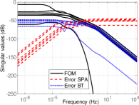
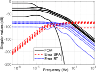
Figure 2: Rail (with $n=20\,209$). Frequency response of FOM and the errors related SPA and BT; using low-rank operations.

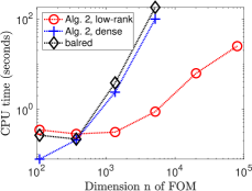
Figure 3: Rail with varying dimension $n$. CPU times for SPA realized by Algorithm 2 (either using low-rank or dense operations) and Matlab built-in function balred ($r=12$ for all ROMs).

The numerical studies are performed, from here on, for a benchmark problem described in [10, Section 19] and referred to as Rail, which is given by a semi-discretized heat transfer model of a steel rail. Depending on the underlying mesh resolution of the discretization, the FOM has a dimension $n\in\{109$, $371$, $1\,357$, $5\,177$, $20\,209$, $79\,841\}$. Both the benchmark data as well as the low-rank (ADI-based) Lyapunov equation solvers originate from the MESS toolbox [38]. The numerical results have been generated using MATLAB Version 9.12 (R2022a) on an computer running with an Intel Core i7-8700 CPU with 32.0GB. To allow a better reproducibility of the reported results, the code and the benchmark data are provided in [28].

Notably, regardless of which of the three implementations was chosen for the realization of SPA, almost no effect on the quality of the resulting ROM was observed for the test cases with $n\leq 5\,177$. More precisely, the deviations with respect to the ${{\cal H}_{\infty}}$ norm were below $10^{-10}$. However, larger dimensions could not be considered for the dense solvers, since they did not run to completion on the running machine.

The qualitative behavior of the FOM and the approximation errors for SPA and BT are illustrated in the frequency domain in Figure 2 for two different choices of the ROM order $r\in\{12,36\}$. As to be expected, SPA performs better in the lower frequency range, while BT is better in the higher frequency range. The maximum frequency-domain errors of the methods are fairly similar, ranging at about $-50db$ for $r=12$ and at $-75db$ for $r=36$.

However, the computational times of the different SPA implementations vary significantly as illustrated in Figure 3. While the two variants using dense solvers are almost the same in this respect, the low-rank implementation Alg. 2, low-rank is already seven times faster for a FOM dimension of $n=1\,357$, i.e., $0.3$ seconds compared to $2.8$ seconds. The difference becomes even more pronounced for larger dimensions. The sparse solver is even faster for $n=79\,841$ than balred for $n=5\,177$. (Alg. 2, low-rank for $n=79\,841$: $25.0$ seconds versus balred for $n=5\,177$: $181.2$ seconds). Larger dimensions are not feasible for balred due to the internal memory limits of the computing machine. It is to be noted that the very large memory demand of the dense solvers is a strong limitation in the large-scale setting.

5 Data-driven implementation of balancing-related methods

In [22], it was shown that BT can be realized (approximately) in a non-intrusive, data-driven manner. There, ”data” are transfer function evaluations. This is fundamentally different to the other data-driven BT approaches in [31, 43, 37, 33], which require snapshots of the full state. The main idea underlying the approach in [22] is to make use only implicitly of quadrature approximations of the two system Gramians for the construction of a low-order approximately balanced model.

The novel contribution of this part is to derive a similar data-driven adaptation of SPA (or QuadSPA). Since it follows similar principles as [22], we set the stage in Section 5.1 by going over the basic construction underlying the latter. In Section 5.2 QuadSPA is derived, and its numerical performance is examined in Section 6.

Since we are interested in realization-free approaches, we may assume ${\textbf{E}}={\textbf{I}}$ from here on. This modification carries over to the FOM, i.e., instead of (1), we have

$$\dot{{\textbf{x}}}(t) ={\textbf{A}}\,{\textbf{x}}(t)+{\textbf{B}}\,{\textbf{u}}(t),\hskip 34.14322pt{\textbf{y}}(t)={\textbf{C}}{\textbf{x}}(t)+{\textbf{D}}{\textbf{u}}(t).$$

5.1 Data-driven Balanced Truncation

Following the BT implementation in Algorithm 1 (with ${\textbf{E}}={\textbf{I}}$), square-root factors U, and L of the Gramians are defined, and their product is approximated by a singular value decomposition, according to

$${\textbf{L}}^{T}{\textbf{U}}\approx{\textbf{Z}}_{1}{\textbf{S}}_{1}{\textbf{Y}}_{1}^{T},\hskip 28.45274pt{\textbf{S}}_{1}\in{\mathbb{R}}^{r,r}.$$

By the definition of the reduction bases ${\textbf{W}}_{r}={\textbf{L}}{\textbf{Z}}_{1}{\textbf{S}}_{1}^{-1/2}$ and ${\textbf{V}}_{r}={\textbf{U}}{\textbf{Y}}_{1}{\textbf{S}}_{1}^{-1/2}$ (Step 3 in the algorithm), the matrices of the ROM realization are expressed as

$${\textbf{A}}_{r} ={\textbf{W}}_{r}^{T}{\textbf{A}}{\textbf{V}}_{r}={\textbf{S}}_{1}^{-1/2}{\textbf{Z}}_{1}^{T}\,({\textbf{L}}^{T}{\textbf{A}}{\textbf{U}})\,{\textbf{Y}}_{1}{\textbf{S}}_{1}^{-1/2}, {\textbf{B}}_{r}={\textbf{W}}_{r}^{T}{\textbf{B}}={\textbf{S}}_{1}^{-1/2}{\textbf{Z}}_{1}^{T}\,({\textbf{L}}^{T}{\textbf{B}}),$$

$${\textbf{C}}_{r} ={\textbf{C}}{\textbf{V}}_{r}=({\textbf{C}}{\textbf{U}})\,{\textbf{Y}}_{1}{\textbf{S}}_{1}^{-1/2}.$$

By the latter relations, we observe that the ROM is fully characterized in terms of the following key quantities:

$${\textbf{L}}^{T}{\textbf{U}},\hskip 8.5359pt{\textbf{L}}^{T}{\textbf{A}}{\textbf{U}},\hskip 8.5359pt{\textbf{L}}^{T}{\textbf{B}}\hskip 8.5359pt\text{and}\hskip 8.5359pt{\textbf{C}}{\textbf{U}}.$$ (10)

These matrices can be approximated well from input-output data, as it is shown next.

The starting point is a quadrature approximation of the Gramians in the frequency domain. Let ${\dot{\imath\imath}}$ be the complex unit with ${\dot{\imath\imath}}^{2}=-1$. Then, the controllability Gramian P and the observability Gramian Q. (i.e., the solutions to (4)) can be expressed as

$$\begin{aligned} {\textbf{P}}&=\frac{1}{2\pi}\int_{-\infty}^{\infty}({\dot{\imath\imath}}\zeta{\textbf{I}}-{\textbf{A}})^{-1}{\textbf{B}}{\textbf{B}}^{T}(-{\dot{\imath\imath}}\zeta{\textbf{I}}^{T}-{\textbf{A}}^{T})^{-1}d\zeta,\\ {\textbf{Q}}&=\frac{1}{2\pi}\int_{-\infty}^{\infty}(-{\dot{\imath\imath}}\omega{\textbf{I}}-{\textbf{A}}^{T})^{-1}{\textbf{C}}{\textbf{C}}^{T}({\dot{\imath\imath}}\omega{\textbf{I}}-{\textbf{A}})^{-1}d\omega.\end{aligned}$$

We consider first a numerical quadrature rule that approximates the frequency integral defining the controllability Gramian, producing an approximate Gramian $\widetilde{{\textbf{P}}}$:

$${\textbf{P}}\approx\widetilde{{\textbf{P}}}=\sum_{k=1}^{{{}{J}}}\rho_{k}^{2}({\dot{\imath\imath}}\omega_{k}{\textbf{I}}-{\textbf{A}})^{-1}{\textbf{B}}{\textbf{B}}^{T}(-{\dot{\imath\imath}}\omega_{k}{\textbf{I}}^{T}-{\textbf{A}}^{T})^{-1}$$ (11)

Hereby, $\omega_{k}$ and $\rho_{k}^{2}$ denote the quadrature nodes and quadrature weights, respectively. Thus, $\rho_{k}$ are, by construction, the square-roots of the quadrature weights. Evidently, we may decompose the quadrature-based Gramian approximation as $\widetilde{{\textbf{P}}}=\widetilde{{\textbf{U}}}\widetilde{{\textbf{U}}}^{*}$ with a square-root factor $\widetilde{{\textbf{U}}}\in\mathbb{C}^{n\times{{}{J}}m}$ defined as

$$\widetilde{{\textbf{U}}}=\left[\,\rho_{1}({\dot{\imath\imath}}\omega_{1}{\textbf{I}}-{\textbf{A}})^{-1}{\textbf{B}}\quad\cdots\quad\rho_{{}{J}}({\dot{\imath\imath}}\omega_{{}{J}}{\textbf{I}}-{\textbf{A}})^{-1}{\textbf{B}}\right].$$ (12)

Note that both P and its quadrature approximation, $\widetilde{{\textbf{P}}}$, are real-valued matrices, yet the explicit square-root factor, $\widetilde{{\textbf{U}}}$, is overtly complex and subsequent computation engages complex floating point arithmetic.

Similarly, a quadrature approximation of Q is defined by

$${\textbf{Q}}\approx\widetilde{{\textbf{Q}}}=\sum_{j=1}^{{{}{J}}}{\varphi}_{j}^{2}(-{\dot{\imath\imath}}{\zeta}_{j}{\textbf{I}}^{T}-{\textbf{A}}^{T})^{-1}{\textbf{C}}^{T}{\textbf{C}}({\dot{\imath\imath}}{\zeta}_{j}{\textbf{I}}-{\textbf{A}})^{-1},$$

with quadrature points ${\zeta}_{j}$ and quadrature weights ${\varphi}_{j}^{2}$. (For convenience we assume the number of quadrature points to be the same for Q and P.) The corresponding square-root factor decomposition reads $\widetilde{{\textbf{Q}}}=\widetilde{{\textbf{L}}}\widetilde{{\textbf{L}}}^{*}$ where

$$\widetilde{{\textbf{L}}}^{*}=\left[\begin{matrix}{\varphi}_{1}{\textbf{C}}({\dot{\imath\imath}}{\zeta}_{1}{\textbf{I}}-{\textbf{A}})^{-1}\\ \vdots\\ {\varphi}_{{}{J}}{\textbf{C}}({\dot{\imath\imath}}{\zeta}_{{}{J}}{\textbf{I}}-{\textbf{A}})^{-1}\end{matrix}\right]\in\mathbb{C}^{{{}{J}}p\times n}.$$ (13)

For a concise notation in the multi-input multi-output setting, the following two technical definitions are useful.

Definition 5.1.

Let ${\textbf{X}}\in{\mathbb{C}}^{{{}{J}}p\times{{}{J}}m}$. Then, for $1\leq k,j\leq{{}{J}}$, we say that the $(k,j)$th block $(p,m)$ entry of matrix X is a matrix in ${\mathbb{C}}^{p\times m}$, denoted with ${\textbf{X}}_{k,j}$, for which its $p$ rows are a subset of the rows of matrix X, indexed from $(k-1)p+1$ to $kp$. Additionally, the $m$ columns of the matrix ${\textbf{X}}_{k,j}$ are a subset of the columns of the matrix X, indexed from $(k-1)m+1$ to $km$.

It is to be noted that in Definition 5.1, if $m=p=1$ (corresponding to the SISO case), then ${\textbf{X}}_{k,j}$ is nothing else but the $(k,j)$th scalar (or $(1,1)$) entry of matrix ${\textbf{X}}\in{\mathbb{C}}^{{{}{J}}\times{{}{J}}}$.

Definition 5.2.

Let ${\textbf{X}}\in{\mathbb{C}}^{{{}{J}}p\times m}$. Then, for $1\leq k\leq{{}{J}}$, we say that the $k$th block $(p,m)$ entry of matrix X is a matrix in ${\mathbb{C}}^{p\times m}$, denoted with ${\textbf{X}}_{k}$, for which its $p$ rows are a subset of the rows of matrix X, indexed from $(k-1)p+1$ to $kp$. Additionally, the $m$ columns of matrix ${\textbf{x}}_{k}$ are exactly the same as those of matrix X. (An equivalent definition can be formulated for ${\textbf{X}}\in{\mathbb{C}}^{p\times{{}{J}}m}$; however, for brevity sake, we skip the details here.)

Algorithm 3 Quadrature-based Balanced Truncation (QuadBT)

Require: -Transfer function of FOM: $\mathbf{H}(s)$;
       -Two sets of quadrature rules for approximating an integral of the form $1/(2\pi)\int_{-\infty}^{\infty}f(s)ds$:
         given by $\omega_{k}$, $\rho_{k}$, respectively ${\zeta}_{j}$, ${\varphi}_{j}$ for for $k,j=1,2,\ldots,{{}{J}}$ (assuming $\omega_{k}\neq{\zeta}_{j}$)
       reduced dimension $r$, $1\leq r\leq{{}{J}}\min(m,p)$.

Ensure: ROM: $\tilde{{{\textbf{A}}}}_{r}\in\mathbb{R}^{r\times r},\ \tilde{{{\textbf{B}}}}_{r}\in\mathbb{R}^{r\times m},\tilde{{{\textbf{C}}}}_{r}\in\mathbb{R}^{p\times r}$ and  $\tilde{{{\textbf{D}}}}_{r}\in{\mathbb{R}}^{p\times m}.$

1:  Determine feedtrough term ${\textbf{D}}=\lim_{s\to\infty}\mathbf{H}(s)$.

2:   Evaluate the strictly proper transfer function ${\mathbf{H}}_{\infty}:s\mapsto\mathbf{H}(s)-{\textbf{D}}$ at $\{{\mathbf{H}}_{\infty}({\dot{\imath\imath}}\omega_{j})\}_{j=1}^{{{}{J}}}$ and $\{{\mathbf{H}}_{\infty}({\dot{\imath\imath}}{\zeta}_{k})\}_{k=1}^{{{}{J}}}$. Using the samples and the quadrature weights, construct $\boldsymbol{\widetilde{\mathbf{{N}}}},\boldsymbol{\widetilde{\mathbf{{M}}}}$, $\widetilde{\mathbb{T}}$, and $\widetilde{\mathbf{{G}}}$ as in Proposition 5.1.

3:  Compute the SVD of matrix $\widetilde{\mathbf{{N}}}\in{\mathbb{C}}^{{{}{J}}p\times{{}{J}}m}$:

$$\widetilde{\mathbf{{N}}}=\left[\begin{matrix}\widetilde{{\textbf{Z}}}_{1}&\widetilde{{\textbf{Z}}}_{2}\end{matrix}\right]\left[\begin{matrix}\widetilde{{\textbf{S}}}_{1}&\\ &\widetilde{{\textbf{S}}}_{2}\end{matrix}\right]\left[\begin{matrix}\widetilde{{\textbf{Y}}}_{1}^{*}\\ \widetilde{{\textbf{Y}}}_{2}^{*}\end{matrix}\right],$$

where $\widetilde{{\textbf{S}}}_{1}\in\mathbb{R}^{r\times r}$ and $\widetilde{{\textbf{S}}}_{2}\in\mathbb{R}^{({{}{J}}p-r)\times({{}{J}}m-r)}$.

4:  Construct the reduced order matrices:

$$\tilde{{{\textbf{A}}}}_{r}=\widetilde{{\textbf{S}}}_{1}^{-1/2}\widetilde{{\textbf{Z}}}_{1}^{*}\widetilde{\mathbf{{M}}}\ \widetilde{{\textbf{Y}}}_{1}\widetilde{{\textbf{S}}}_{1}^{-1/2},\hskip 5.69046pt\tilde{{{\textbf{B}}}}_{r}=\widetilde{{\textbf{S}}}_{1}^{-1/2}\widetilde{{\textbf{Z}}}_{1}^{*}\widetilde{\mathbb{T}},\tilde{{{\textbf{C}}}}_{r}=\widetilde{\mathbf{{G}}}^{T}\widetilde{{\textbf{Y}}}_{1}\widetilde{{\textbf{S}}}_{1}^{-1/2},\hskip 5.69046pt\text{and}\hskip 5.69046pt\tilde{{{\textbf{D}}}}_{r}={\textbf{D}}$$

By the latter considerations and noticing that $\mathbf{H}(\infty)={\textbf{D}}$, it can be seen that the key quantities in (10) can be approximated by transfer function evaluations.

Proposition 5.1.

Let $\widetilde{{\textbf{U}}}$ and $\widetilde{{\textbf{L}}}$ be as defined in (12) and (13), whereby the quadrature points $\omega_{k}\neq{\zeta}_{j}$ are distinct for $1\leq k,j\leq{{}{J}}$. Also, let

$${\mathbf{H}}_{\infty}(s)={\textbf{C}}(s{\textbf{I}}-{\textbf{A}})^{-1}{\textbf{B}}=\mathbf{H}(s)-\lim_{\tilde{s}\to\infty}\mathbf{H}(\tilde{s}).$$

Define the matrices $\widetilde{\mathbf{{N}}}=\widetilde{{\textbf{L}}}^{*}\widetilde{{\textbf{U}}}\in{\mathbb{C}}^{{{}{J}}p\times{{}{J}}m}$ and $\widetilde{\mathbf{{M}}}=\widetilde{{\textbf{L}}}^{*}{\textbf{A}}\widetilde{{\textbf{U}}}\in{\mathbb{C}}^{{{}{J}}p\times{{}{J}}m}$.
Then, for $1\leq k,j\leq{{}{J}}$, the $(k,j)$th block $(p,m)$ entries of matrices $\widetilde{\mathbf{{N}}}$ and $\widetilde{\mathbf{{M}}}$, respectively read as (following Definition 5.1):

$$\widetilde{\mathbf{{N}}}_{k,j} =-\rho_{k}{\varphi}_{j}\displaystyle\frac{{\mathbf{H}}_{\infty}({\dot{\imath\imath}}\omega_{k})-{\mathbf{H}}_{\infty}({\dot{\imath\imath}}\omega_{j})}{{\dot{\imath\imath}}\omega_{k}-{\dot{\imath\imath}}\omega_{j}},$$

$$\widetilde{\mathbf{{M}}}_{k,j} =-\rho_{k}{\varphi}_{j}\displaystyle\frac{{\dot{\imath\imath}}\omega_{k}{\mathbf{H}}_{\infty}({\dot{\imath\imath}}\omega_{k})-{\dot{\imath\imath}}{\zeta}_{j}{\mathbf{H}}_{\infty}({\dot{\imath\imath}}\omega_{j})}{{\dot{\imath\imath}}\omega_{k}-{\dot{\imath\imath}}\omega_{j}}.$$

Likewise, defining $\widetilde{\mathbb{T}}=\widetilde{{\textbf{L}}}^{*}{\textbf{B}}\in{\mathbb{C}}^{{{}{J}}p\times m}$ and $\widetilde{\mathbf{{G}}}^{T}={\textbf{C}}^{T}\widetilde{{\textbf{U}}}\in{\mathbb{C}}^{p\times{{}{J}}m}$, and by following Definition 5.2, we find

$$\widetilde{\mathbb{T}}_{k} =\rho_{k}{\mathbf{H}}_{\infty}({\dot{\imath\imath}}\omega_{k}),\hskip 8.5359pt\text{and}\hskip 8.5359pt\widetilde{\mathbf{{G}}}_{j}={\varphi}_{j}{\mathbf{H}}_{\infty}({\dot{\imath\imath}}\omega_{j}),\hskip 8.5359pt\text{for}\ 1\leq k,j\leq{{}{J}}.$$

More details and various extensions (using time-domain data, for discrete-time systems, etc.) can be found in [22]. Based on Proposition 5.1, the data-driven adaptation of BT can be implemented, as it is shown in Algorithm 3. A proof of the proposition can be found in Appendix A; this is indeed useful for setting up the stage for the derivations of the novel QuadSPA presented in the next section.

5.2 Data-driven Singular Perturbation Approximation

The formulation of the novel data-driven QuadSPA implementation is presented here. Similarly as for the low-rank implementation of SPA (Section 4.2), we rely on a construction based on the alternative characterization of Proposition 3.2 and illustrated in Figure 1. First, an intermediate ROM $(\widetilde{\mathfrak{{A}}}_{r},\widetilde{\mathfrak{{B}}}_{r},\widetilde{\mathfrak{{C}}}_{r},\widetilde{\mathfrak{{D}}}_{r})$ approximating the reciprocal counterpart of the FOM is constructed. Then, by applying the reciprocal transformation of this low-dimensional intermediate ROM, we obtain the QuadSPA reduced system approximating the FOM.

However, the intermediate ROM is constructed from data here, following a similar quadrature approximation as in the data-driven BT, cf. Section 5.1. This approximation requires a careful choice of quadrature rule. To derive an appropriate one, we rewrite the frequency representations of the reciprocal Gramians $\mathfrak{{P}}$ and $\mathfrak{{Q}}$ in terms of evaluations of the original transfer function in (2). Let

$${\mathfrak{K}}:{\mathbb{C}}\to{\mathbb{C}}^{n,n},\qquad{\mathfrak{K}}(s)=(s{\textbf{I}}-\mathfrak{{A}})^{-1},$$

so that the strictly proper part of the reciprocal transfer function $s\mapsto{\mathfrak{H}}(s)-{\mathfrak{H}}(\infty)$ can be equivalently expressed as $s\mapsto\mathfrak{{C}}{\mathfrak{K}}(s)\mathfrak{{B}}$. Similarly to the derivation of the data-driven BT, we consider the frequency representations of the Gramians. The reciprocal controllability Gramian reads

$$\begin{split}\mathfrak{{P}}&=\frac{1}{2\pi}\int_{-\infty}^{\infty}{\mathfrak{K}}({\dot{\imath\imath}}\zeta)\mathfrak{{B}}\mathfrak{{B}}^{T}{\mathfrak{K}}(-{\dot{\imath\imath}}\zeta)^{T}d\zeta=\frac{1}{2\pi}\int_{-\infty}^{\infty}{\mathfrak{K}}\left(\frac{1}{{\dot{\imath\imath}}\zeta}\right)\mathfrak{{B}}\mathfrak{{B}}^{T}{\mathfrak{K}}\left(\frac{1}{-{\dot{\imath\imath}}\zeta}\right)^{T}\frac{1}{\zeta^{2}}d\zeta,\end{split}$$

whereby the last equality follows by using integration with the substitution $s\to-1/s$ on ${\mathfrak{{\mathbf{{F}}}}}(\zeta):=\frac{1}{2\pi}{\mathfrak{K}}({\dot{\imath\imath}}\zeta)\mathfrak{{B}}\mathfrak{{B}}^{T}{\mathfrak{K}}(-{\dot{\imath\imath}}\zeta)^{T}$, according to

$$\int_{-\infty}^{\infty}{\mathfrak{{\mathbf{{F}}}}}(\zeta)d\zeta =\int_{-\infty}^{0}{\mathfrak{{\mathbf{{F}}}}}(\zeta)d\zeta+\int_{0}^{\infty}{\mathfrak{{\mathbf{{F}}}}}(\zeta)d\zeta$$

$$=\int_{0}^{\infty}{\mathfrak{{\mathbf{{F}}}}}\left(-\frac{1}{\zeta}\right)\frac{1}{\zeta^{2}}d\zeta+\int_{-\infty}^{0}{\mathfrak{{\mathbf{{F}}}}}\left(-\frac{1}{\zeta}\right)\frac{1}{\zeta^{2}}d\zeta=\int_{-\infty}^{\infty}{\mathfrak{{\mathbf{{F}}}}}\left(-\frac{1}{\zeta}\right)\frac{1}{\zeta^{2}}d\zeta.$$

Based on the reformulation, we consider the following approximation by quadrature,

$$\begin{split}\mathfrak{{P}}&\approx\tilde{{\mathfrak{{P}}}}=\sum_{k=1}^{{{}{J}}}\left(\frac{\rho_{k}}{\omega_{k}}\right)^{2}{\mathfrak{K}}\left(\frac{1}{{\dot{\imath\imath}}\omega_{k}}\right)\mathfrak{{B}}\mathfrak{{B}}^{T}{\mathfrak{K}}\left(\frac{1}{-{\dot{\imath\imath}}\omega_{k}}\right)^{T},\end{split}$$

with quadrature nodes $\omega_{k}$ and weights $\rho_{k}^{2}$. This is in analogy to the approximation provided by (11). We define a square-root factor $\widetilde{\mathfrak{{U}}}$, which fulfills $\widetilde{\mathfrak{{P}}}=\widetilde{\mathfrak{{U}}}\widetilde{\mathfrak{{U}}}^{*}$, as

$$\widetilde{\mathfrak{{U}}}=\left[\,\frac{\rho_{1}}{\omega_{1}}{\mathfrak{K}}\left(\frac{1}{{\dot{\imath\imath}}\omega_{1}}\right)\mathfrak{{B}}\quad\cdots\quad\frac{\rho_{{}{J}}}{\omega_{{}{J}}}{\mathfrak{K}}\left(\frac{1}{{\dot{\imath\imath}}\omega_{{}{J}}}\right)\mathfrak{{B}}\right]\in\mathbb{C}^{n\times{{}{J}}m}.$$ (14)

Similarly, the reciprocal observability Gramian is approximated by quadrature

$$\begin{split}\mathfrak{{Q}}\approx\widetilde{\mathfrak{{Q}}}=\sum_{k=1}^{{{}{J}}}\left(\frac{{\varphi}_{j}}{{\zeta}_{j}}\right)^{2}{\mathfrak{K}}\left(\frac{1}{-{\dot{\imath\imath}}{\zeta}_{j}}\right)^{T}\mathfrak{{C}}^{T}\mathfrak{{C}}{\mathfrak{K}}\left(\frac{1}{{\dot{\imath\imath}}{\zeta}_{j}}\right),\end{split}$$

with quadrature points and weights ${\zeta}_{j}$ and ${\varphi}_{j}^{2}$, respectively. The corresponding square-root factor decomposition reads $\widetilde{\mathfrak{{Q}}}=\widetilde{\mathfrak{{L}}}\widetilde{\mathfrak{{L}}}^{*}$, where

$$\widetilde{\mathfrak{{L}}}^{*}=\left[\begin{matrix}\frac{{\varphi}_{1}}{{\zeta}_{1}}\mathfrak{{C}}{\mathfrak{K}}\left(\frac{1}{{\dot{\imath\imath}}{\zeta}_{1}}\right)\\ \vdots\\ \frac{{\varphi}_{{}{J}}}{{\zeta}_{{}{J}}}\mathfrak{{C}}{\mathfrak{K}}\left(\frac{1}{{\dot{\imath\imath}}{\zeta}_{{}{J}}}\right)\\ \end{matrix}\right]\in\mathbb{C}^{{{}{J}}p\times n}.$$ (15)

Certain key quantities of the reciprocal system can be directly approximated from data, as the following result shows. The construction is similar to the one used in Proposition 5.1.

Proposition 5.2.

Let $\widetilde{\mathfrak{{U}}}$ and $\widetilde{\mathfrak{{L}}}$ be as defined in (14) and (15), whereby the quadrature-points $\omega_{k}\neq{\zeta}_{j}$ are distinct and nonzero for $1\leq k,j\leq{{}{J}}$. Also, let

$${\mathbf{H}}_{0}:{\mathbb{C}}\to{\mathbb{C}}^{p,m},\qquad{\mathbf{H}}_{0}({s})=\mathbf{H}(s)-\mathbf{H}(0).$$

Define the matrices $\widetilde{\mathfrak{{N}}}=\widetilde{\mathfrak{{L}}}^{*}\widetilde{\mathfrak{{U}}}\in{\mathbb{C}}^{{{}{J}}p\times{{}{J}}m}$ and $\widetilde{\mathfrak{{M}}}=\widetilde{\mathfrak{{L}}}^{*}\mathfrak{{A}}\widetilde{\mathfrak{{U}}}\in{\mathbb{C}}^{{{}{J}}p\times{{}{J}}m}$. Then, for $1\leq k,j\leq{{}{J}}$, the $(k,j)$th block $(p,m)$ entries of matrices $\widetilde{\mathfrak{{N}}}$ and $\widetilde{\mathfrak{{M}}}$, respectively read (following Definition 5.1) as

$$\widetilde{\mathfrak{{N}}}_{k,j} =-\rho_{k}{\varphi}_{j}\displaystyle\frac{{\mathbf{H}}_{0}({\dot{\imath\imath}}\omega_{k})-{\mathbf{H}}_{0}({\dot{\imath\imath}}{\zeta}_{j})}{{\dot{\imath\imath}}\omega_{k}-{\dot{\imath\imath}}{\zeta}_{j}},$$

$$\widetilde{\mathfrak{{M}}}_{k,j} =-\rho_{k}{\varphi}_{j}\displaystyle\frac{({\dot{\imath\imath}}\omega_{k})^{-1}{\mathbf{H}}_{0}({\dot{\imath\imath}}\omega_{k})-({\dot{\imath\imath}}{\zeta}_{j})^{-1}{\mathbf{H}}_{0}({\dot{\imath\imath}}{\zeta}_{j})}{{\dot{\imath\imath}}\omega_{k}-{\dot{\imath\imath}}{\zeta}_{j}}.$$

Likewise, defining $\widetilde{\mathfrak{{T}}}=\widetilde{\mathfrak{{L}}}^{*}\mathfrak{{B}}\in{\mathbb{C}}^{{{}{J}}p\times m}$ and $\widetilde{\mathfrak{{G}}}^{T}=\mathfrak{{C}}\widetilde{\mathfrak{{U}}}\in{\mathbb{C}}^{p\times{{}{J}}m}$ we find

$$\widetilde{\mathfrak{{T}}}_{k} =\frac{\rho_{k}}{\omega_{k}}{\mathbf{H}}_{0}({\dot{\imath\imath}}\omega_{k}),\hskip 8.5359pt\text{and}\hskip 8.5359pt\widetilde{\mathfrak{{G}}}_{j}=\frac{{\varphi}_{j}}{{\zeta}_{j}}{\mathbf{H}}_{0}({\dot{\imath\imath}}{\zeta}_{j}),\hskip 8.5359pt\text{for}\ 1\leq k,j\leq{{}{J}}.$$

Proof.

Only for this proof, we introduce the abbreviations ${\nu}=({\dot{\imath\imath}}\omega_{k})^{-1}$ and ${\mu}=({\dot{\imath\imath}}{\zeta}_{j})^{-1}$. A small calculation shows that

$${\mathfrak{K}}({\nu}){\mathfrak{K}}({\mu})=\frac{1}{{\nu}-{\mu}}{\mathfrak{K}}({\nu})\left[({\nu}{\textbf{I}}-\mathfrak{{A}})-({\mu}{\textbf{I}}-\mathfrak{{A}})\right]{\mathfrak{K}}({\mu})=-\frac{1}{{\nu}-{\mu}}\left({\mathfrak{K}}({\nu})-{\mathfrak{K}}({\mu})\right).$$

By the latter, and $\mathfrak{{C}}{\mathfrak{K}}({\nu})\mathfrak{{B}}={\mathbf{H}}_{0}({1/{\nu}})={\mathbf{H}}_{0}({\dot{\imath\imath}}\omega_{k})$, and $\mathfrak{{C}}{\mathfrak{K}}({\mu})\mathfrak{{B}}={\mathbf{H}}_{0}({\dot{\imath\imath}}{\zeta}_{j})$, it follows

$$\widetilde{\mathfrak{{N}}}_{k,j} =(\rho_{k}/\omega_{k})({\varphi}_{j}/{\zeta}_{j})\,\mathfrak{{C}}{\mathfrak{K}}({\nu}){\mathfrak{K}}({\mu})\mathfrak{{B}}=-\rho_{k}{\varphi}_{j}\frac{1}{\omega_{k}{\zeta}_{j}({\nu}-{\mu})}\mathfrak{{C}}\left[{\mathfrak{K}}({\nu})-{\mathfrak{K}}({\mu})\right]\mathfrak{{B}}$$

$$=-\rho_{k}{\varphi}_{j}\frac{{\mathbf{H}}_{0}({\dot{\imath\imath}}\omega_{k})-{\mathbf{H}}_{0}({\dot{\imath\imath}}{\zeta}_{j})}{{\dot{\imath\imath}}\omega_{k}-{\dot{\imath\imath}}{\zeta}_{j}},$$

whereby $\omega_{k}{\zeta}_{j}({\nu}-{\mu})={\dot{\imath\imath}}\omega_{k}-{\dot{\imath\imath}}{\zeta}_{j}$ was used in the last step. Moreover using the relation

$${\mathfrak{K}}({\nu})\mathfrak{{A}}{\mathfrak{K}}({\mu})=-\frac{1}{{\nu}-{\mu}}\left[{\nu}{\mathfrak{K}}({\nu})-{\mu}{\mathfrak{K}}({\mu})\right],$$

we can show in a similar manner that

$$\widetilde{\mathfrak{{M}}}_{k,j} =(\rho_{k}/\omega_{k})({\varphi}_{j}/{\zeta}_{j})\,\mathfrak{{C}}\left({\mathfrak{K}}({\nu})\mathfrak{{A}}{\mathfrak{K}}({\mu})\right)\mathfrak{{B}}=-\rho_{k}{\varphi}_{j}\frac{1}{\omega_{k}{\zeta}_{j}({\nu}-{\mu})}\mathfrak{{C}}\left({\nu}{\mathfrak{K}}({\nu})-{\mu}{\mathfrak{K}}({\mu})\right)\mathfrak{{B}}$$

$$=-\rho_{k}{\varphi}_{j}\displaystyle\frac{({\dot{\imath\imath}}\omega_{k})^{-1}{\mathbf{H}}_{0}({\dot{\imath\imath}}\omega_{k})-({\dot{\imath\imath}}{\zeta}_{j})^{-1}{\mathbf{H}}_{0}({\dot{\imath\imath}}{\zeta}_{j})}{{\dot{\imath\imath}}\omega_{k}-{\dot{\imath\imath}}{\zeta}_{j}}.$$

The explicit representations of $\widetilde{\mathfrak{{T}}}$ and $\widetilde{\mathfrak{{G}}}$ (as data matrices) are easily derived, since

$$\widetilde{\mathfrak{{T}}}_{k} =(\rho_{k}/\omega_{k})\,\mathfrak{{C}}{\mathfrak{K}}({\dot{\imath\imath}}\omega_{k})\mathfrak{{B}}=\frac{\rho_{k}}{\omega_{k}}{\mathbf{H}}_{0}({\dot{\imath\imath}}\omega_{k}),\ \ \ \widetilde{\mathfrak{{G}}}_{j}=({\varphi}_{j}/{\zeta}_{j})\,\mathfrak{{C}}{\mathfrak{K}}({\dot{\imath\imath}}{\zeta}_{j})\mathfrak{{B}}=\frac{{\varphi}_{j}}{{\zeta}_{j}}{\mathbf{H}}_{0}({\dot{\imath\imath}}{\zeta}_{j}).$$

∎

The main contribution of this section, i.e., the data-driven, realization-free implementation of SPA is summarized in Algorithm 4.

Remark 5.1.

A generalized version of Proposition 5.2 omitting the assumption $\omega_{k}\neq{\zeta}_{j}$ for all $j,k$ can be derived, but it requires evaluations of the derivative of the transfer function, see Appendix B for details.

Algorithm 4 Quadrature-based Singular Perturbation Approximation (QuadSPA)

Require: -Transfer function of FOM: $\mathbf{H}(s)$;
       -Two sets of quadrature rules for approximating an integral of the form $1/(2\pi)\int_{-\infty}^{\infty}f(s)ds$:
         given by $\omega_{k}$, $\rho_{k}$, respectively ${\zeta}_{j}$, ${\varphi}_{j}$ for for $k,j=1,2,\ldots,{{}{J}}$ (assuming $\omega_{k}\neq{\zeta}_{j}$)
       -reduced dimension $r$, $1\leq r\leq\min({{}{J}}p,{{}{J}}m)$.

Ensure: ROM: $\tilde{{{\textbf{A}}}}_{r}\in\mathbb{R}^{r\times r},\,\tilde{{{\textbf{B}}}}_{r}\in{\mathbb{R}}^{r\times m},\,\tilde{{{\textbf{C}}}}_{r}\in{\mathbb{R}}^{p\times r}$, and  $\tilde{{{\textbf{D}}}}_{r}\in{\mathbb{R}}^{p\times m}$

1:  Determine the moment ${\textbf{D}}_{0}=\mathbf{H}(0)$.

2:   Evaluate the modified transfer function ${\mathbf{H}}_{0}:s\mapsto\mathbf{H}(s)-{\textbf{D}}_{0}$ at $\{{\mathbf{H}}_{0}({\dot{\imath\imath}}\omega_{k})\}_{k=1}^{{{}{J}}}$ and $\{{\mathbf{H}}_{0}({\dot{\imath\imath}}{\zeta}_{j})\}_{j=1}^{{{}{J}}}$. Using the samples and the quadrature weights, construct the data matrices $\widetilde{\mathfrak{{N}}},\widetilde{\mathfrak{{M}}}$, $\widetilde{\mathfrak{{T}}}$, and $\widetilde{\mathfrak{{G}}}$ as in Proposition 5.2.

3:  Compute the SVD of matrix $\widetilde{\mathfrak{{N}}}\in{\mathbb{C}}^{{{}{J}}p\times{{}{J}}m}$:

$$\widetilde{\mathfrak{{N}}}=\left[\begin{matrix}\widetilde{{\textbf{Z}}}_{1}&\widetilde{{\textbf{Z}}}_{2}\end{matrix}\right]\left[\begin{matrix}\widetilde{{\textbf{S}}}_{1}&\\ &\widetilde{{\textbf{S}}}_{2}\end{matrix}\right]\left[\begin{matrix}\widetilde{{\textbf{Y}}}_{1}^{*}\\ \widetilde{{\textbf{Y}}}_{2}^{*}\end{matrix}\right],$$

where $\widetilde{{\textbf{S}}}_{1}\in\mathbb{R}^{r\times r}$ and $\widetilde{{\textbf{S}}}_{2}\in\mathbb{R}^{({{}{J}}p-r)\times({{}{J}}m-r)}$.

4:  Construct the intermediate reduced order matrices:

$$\widetilde{\mathfrak{{A}}}_{r}=\widetilde{{\textbf{S}}}_{1}^{-1/2}\widetilde{{\textbf{Z}}}_{1}^{*}\widetilde{\mathfrak{{M}}}\ \widetilde{{\textbf{Y}}}_{1}\widetilde{{\textbf{S}}}_{1}^{-1/2}\widetilde{\mathfrak{{B}}}_{r}=\widetilde{{\textbf{S}}}_{1}^{-1/2}\widetilde{{\textbf{Z}}}_{1}^{*}\widetilde{\mathfrak{{T}}},\hskip 5.69046pt\widetilde{\mathfrak{{C}}}_{r}=\widetilde{\mathfrak{{G}}}^{T}\widetilde{{\textbf{Y}}}_{1}\widetilde{{\textbf{S}}}_{1}^{-1/2},\hskip 5.69046pt\text{and}\hskip 5.69046pt\widetilde{\mathfrak{{D}}}_{r}={{\textbf{D}}_{0}}.$$

5:  Get the ROM by using the reciprocal transformation onto the intermediate ROM, i.e.,

$$\ \tilde{{{\textbf{A}}}}_{r}=\widetilde{\mathfrak{{A}}}_{r}^{-1},\hskip 5.69046pt\tilde{{{\textbf{A}}}}_{r}=\widetilde{\mathfrak{{A}}}_{r}^{-1},\hskip 5.69046pt\tilde{{{\textbf{C}}}}_{r}=-\widetilde{\mathfrak{{C}}}_{r}\widetilde{\mathfrak{{A}}}_{r}^{-1},\hskip 5.69046pt\text{and}\hskip 5.69046pt\tilde{{{\textbf{D}}}}_{r}=\widetilde{\mathfrak{{D}}}_{r}-\widetilde{\mathfrak{{C}}}_{r}\widetilde{\mathfrak{{A}}}_{r}^{-1}\widetilde{\mathfrak{{B}}}_{r}.$$

5.3 Connections of QuadSPA to the Loewner framework

In this section, we aim at revealing some connections that the newly-developed method, QuadSPA, bears with the Loewner framework in [30]. Note that a connection of QuadBT and the Loewner framework has already been made in [22, Section 3.4].

First, by comparing Proposition 5.2 and Proposition 5.1, it can be shown that the data matrix $\widetilde{\mathfrak{{N}}}$ used in QuadSPA and the $\widetilde{\mathbf{{N}}}$ used in QuadBT are exactly the same. They have the interpretation of a diagonally scaled Loewner matrix. The other data matrices, i.e., $\widetilde{\mathbf{{M}}}$ in QuadBT and $\widetilde{\mathfrak{{M}}}$ in QuadSPA relate to (scaled) shifted Loewner matrices. In QuadBT, the shifts are given by ${\dot{\imath\imath}}\omega_{k}$, $1\leq k\leq{{}{J}}$, while in QuadSPA, there one can find the ’inverted shifts’ $({\dot{\imath\imath}}\omega_{k})^{-1}$ instead.

This new context for QuadSPA implies a few observations. First, QuadSPA has a similar computational complexity as the Loewner framework. Choosing more data points ${{}{J}}$ will, in general, imply increasing closeness to the intrusively computed ROM, but will also increase the dimension of the data matrices. Second, the quality of the ROM strongly depends on the quality of the data. When using data sets with perturbed (noisy) measurements, or that contain redundant data (not rich enough to capture the essential properties), the QuadSPA faces similar challenges as the Loewner framework. We intend to study these aspects in more detail, for future works.

As was pointed out in preceding publications, the numerical conditioning of Loewner matrices can be a relevant issue. While the application of quadrature weights (as done in QuadBT and QuadSPA) may improve the conditioning, regularization strategies might still be necessary. Of course, the SVD is an essential step that acts as implicit regularizer, removing the redundancies, provided the truncation order is small enough. Other possible strategies are described in [16], while the robustness of the Loewner approach to noise or perturbations, was investigated in [44, 19].

Also, we note that Algorithm 4 requires a complex SVD, which implies that the resulting ROM realization is, in general complex-valued. However, under the additional assumption that the quadrature points used in the approximation of either Gramian is chosen in complex-conjugate pairs, a real-valued ROM can be enforced. This can be done in a similar manner as was proposed in [2, Section A.1] for the Loewner framework, and in [22, Section 4.1] for QuadBT.

6 Numerical study for the data-driven implementation

In this section, we compare the performance of the newly-proposed quadrature-based, data-driven implementation of SPA according to Algorithm 4, i.e., QuadSPA, with the following model reduction methods from the literature: the intrusive MATLAB built-in implementations of Singular Perturbation Analysis (SPA) and Balanced Truncation (BT), and the quadrature-based implementation of Balanced Truncation, i.e., QuadBT from [22], realized by Algorithm 3.

We consider two benchmark examples, one of low dimension and one of higher dimension; both are available in the MOR-Wiki database, cf. [10]:

1. The LAbuild system models a motion problem in the Los Angeles University hospital building, with 8 floors each having 3 degrees of freedom, namely displacements in the $x$ and $y$ directions, and rotation. The model has $n=48$ states, $m=1$ input, and $p=1$ output. We refer to [18] for more details.

2. The ISS12A system models the structural response of the Russian Service 12A Module of the International Space Station (ISS). The model has $n=1412$ states, $m=3$ inputs, and $p=3$ outputs. We refer to [24] for more details.

For all experiments, the quadrature weights required for QuadSPA and QuadBT are determined according to the given transfer function measurements and the trapezoid quadrature rule. Other choices of quadrature rules are, of course, possible; we refer, e.g., to [14, 15, 22], which consider other more involved quadrature schemes. Extended details are given below but can also be directly comprehended from the MATLAB code used to generate the numerical results, provided in [28].

6.1 LAbuild model

In the first experiment, we choose ${{}{J}}=100$ logarithmically-spaced distributed (sampling) points in the range $\left[10^{0},10^{2}\right]\cdot\imath$. These will act as quadrature nodes. We compare the results of applying the two data-based methods against their intrusive counterparts, i.e., SPA and BT. We fix $r=18$ as the dimension of all four ROMs, for the first experiment. In the left pane of Figure 4, we depict the magnitude of the frequency response for the original system and approximation errors for the 2 ROMs computed with SPA and QuadSPA. In the right pane of Figure 4, we depict the magnitude of the frequency response for the original system and approximation errors for the two ROMs computed with BT and QuadBT. We notice that the SPA-based methods provide worse approximation quality in the higher frequency range, while the BT-based methods provide worse approximation quality in the lower frequency range. Additionally, it is to be noticed that the error curve corresponding to QuadSPA faithfully reproduces that of SPA. The same can be said about BT.

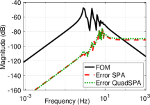
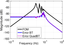
Figure 4: LAbuild. Frequency response of FOM and the errors using SPA and QuadSPA (left) and using BT and QuadBT (right); ${{}{J}}=100$ and $r=18$ is chosen for all ROMs.

In the next experiment, we vary the dimension $r$ of the ROM for all four methods in increments of $6$. The number of data points is fixed to the same value as before, i.e., ${{}{J}}=100$. We compute the ${\cal H}_{\infty}$ norm of the error systems produced by the four model reduction methods, scaled by the ${\cal H}_{\infty}$ norm of the original system. The numerical results are shown in Table 1. As expected, the approximation errors decrease as $r$ increases. Additionally, the quadrature-based methods produce errors comparable to the intrusive counterparts. Actually, for $r\in\{18,24\}$, the QuadSPA method outperforms SPA in term of the ${\cal H}_{\infty}$ norm approximation. However, for $r=12$, the error provided by QuadSPA is much higher than that of SPA (due to a pair of rogue poles), and a similar behavior is noticed for $r=30$, both for QuadSPA and for QuadBT.

Table 1: LAbuild. Relative approximation errors in the ${\cal H}_{\infty}$ norm for varying ROM order $r$ (QuadSPA and QuadBT, with ${{}{J}}=100$).

	$r=6$	$r=12$	$r=18$	$r=24$	$r=30$
SPA	$2.4185\cdot 10^{-1}$	$9.3060\cdot 10^{-2}$	$3.7846\cdot 10^{-2}$	$1.0922\cdot 10^{-2}$	$9.0847\cdot 10^{-4}$
QuadSPA	$2.4971\cdot 10^{-1}$	$5.7480\cdot 10^{-1}$	$3.6713\cdot 10^{-2}$	$1.0836\cdot 10^{-2}$	$3.9822\cdot 10^{-3}$
BT	$2.3084\cdot 10^{-1}$	$1.0317\cdot 10^{-1}$	$3.8312\cdot 10^{-2}$	$1.0613\cdot 10^{-2}$	$9.4410\cdot 10^{-4}$
QuadBT	$2.7935\cdot 10^{-1}$	$1.0442\cdot 10^{-1}$	$3.8193\cdot 10^{-2}$	$1.0285\cdot 10^{-2}$	$4.5524\cdot 10^{-3}$

What we generally observe, is that a higher reduction order $r$ requires more quadrature nodes ${{}{J}}$ in QuadSPA and QuadBT in order to have a similar fidelity as the intrusive methods SPA and BT, respectively. For example, in the latter experiment, we require about ${{}{J}}=300$ points (three times more than before) to ensure that the quadrature-based methods reproduce the quality of the intrusive methods for $r=30$. With this choice of parameters, the relative $\mathcal{H}_{\infty}$ error for QuadSPA is $9.3103\cdot 10^{-4}$ for QuadSPA and $7.9862\cdot 10^{-4}$ for QuadBT, which is very close to the errors of SPA and, interestingly, even slightly better than for BT, respectively, cf. Table 1.

For the next experiment, we vary instead the ${{}{J}}$ parameter between $[20,100]$. We fix the dimension of the ROMs as $r=18$. We compute again the relative approximation errors in the ${\cal H}_{\infty}$ norm, for the two quadrature-based methods. The numerical results are shown in Table 2. As expected, for increasing values of ${{}{J}}$, the relative approximation errors are decreasing for both QuadSPA and QuadBT and typically, they reach the quality of their intrusive counterparts (SPA and BT). Notably, the quadrature-based methods can lead to better results in exceptional cases. This is observed here for ${{}{J}}=100$. However, this does not guarantee, by no means, that for ${{}{J}}>100$, the same trend is valid; e.g., when choosing ${{}{J}}=120$, we noticed that BT outperforms QuadBT.

Table 2: LAbuild. Relative approximation errors in the ${\cal H}_{\infty}$ norm for varying quadrature points ${{}{J}}$, compared to relative errors of intrusive ROMs ($r=18$ for all ROMs).

	${{}{J}}=20$	${{}{J}}=30$	${{}{J}}=50$	${{}{J}}=70$	${{}{J}}=100$
QuadSPA	$3.4571\cdot 10^{-1}$	$3.2915\cdot 10^{-1}$	$6.0762\cdot 10^{-1}$	$7.0414\cdot 10^{-2}$	$3.6713\cdot 10^{-2}$
QuadBT	$7.9048\cdot 10^{-1}$	$3.8459\cdot 10^{-1}$	$1.9527\cdot 10^{-1}$	$9.9991\cdot 10^{-2}$	$3.8193\cdot 10^{-2}$

SPA: $3.7846\cdot 10^{-2}$

BT: $3.8312\cdot 10^{-2}$

6.2 ISS12A model

For the ISS12A model, we first choose ${{}{J}}=1000$ nodes, chosen to be logarithmically-spaced in $[10^{-1},10^{2}]\cdot\imath$. Since the FOM has $3$ inputs and $3$ outputs, the frequency-response plot of it is composed of $3$ curves, i.e., corresponding to the $3$ singular values of ${\textbf{H}}(\imath\omega_{j})\in{\mathbb{C}}^{3\times 3}$, for any frequency point $\omega_{j}$. The reduction order of all ROMs is fixed at $r=100$.

The frequency response plots of the FOM and the reduction errors related to four ROMs are depicted in Figure 5. We notice a good agreement between all responses and a comparable approximation quality for the intrusive and non-intrusive methods. Moreover, as to be expected, the SPA and QuadSPA methods lead to an improved fidelity in the low frequency range, whereas the errors for BT and QuadBT are specifically small for high frequencies.

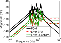
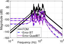
Figure 5: ISS12A. Frequency response of FOM and the errors using SPA and QuadSPA (left) and using BT and QuadBT; ${{}{J}}=1000$ and $r=100$ for all ROMs.

Then, in Figure 6 we depict the configuration of the system poles for the FOM, and for the two ROMs based on quadrature approximations. The dominant poles of the original system seem to be well matched in both cases. Moreover, we would like to mention that the poles in the ROMs occur in complex-conjugated pairs, which is in line with the realness of the fitted models.

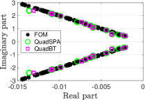
Figure 6: ISS12A. Distribution of system poles for QuadBT and QuadSPA; $r=100$ and ${{}{J}}=1000$ were used.

In the next experiment, we vary the number of points ${{}{J}}$ between $600$ and $1\,000$, and we compute the relative approximation errors in the ${\cal H}_{\infty}$ norm between the original system and the two ROMs, i.e., computed by means of QuadSPA and QuadBT. As expected, the approximation error decreases as ${{}{J}}$ increases, as shown in Table 3.

Table 3: ISS12A. Relative approximation errors in the ${\cal H}_{\infty}$ norm for varying number ${{}{J}}$ of quadrature points (ROM dimension $r=100$).

	${{}{J}}=600$	${{}{J}}=800$	${{}{J}}=1000$
QuadSPA	$5.6244\cdot 10^{-1}$	$1.6758\cdot 10^{-1}$	$3.2221\cdot 10^{-2}$
QuadBT	$6.0982\cdot 10^{-1}$	$4.4826\cdot 10^{-2}$	$3.2171\cdot 10^{-2}$

SPA: $3.3153\cdot 10^{-2}$

BT: $3.2941\cdot 10^{-2}$

Finally, we compute absolute deviations in the ${\cal H}_{\infty}$ norm between the ROMs computed with intrusive model reduction methods (SPA and BT), and their data-based counterparts. We vary ${{}{J}}$ between $200$ and $1\,000$ and compute the ${\cal H}_{\infty}$ quantities in Table 4. As the number of data points is increased, the deviation between the quadrature-based implementations QuadSPA and QuadBT and their intrusive implementation generally decreases and becomes negligible compared to the reduction error of the method.

Table 4: ISS12A. ${\cal H}_{\infty}$ norm deviations between intrusive and quadrature-based methods for varying ${{}{J}}$ (ROM dimension is $r=100$.)

	${{}{J}}=200$	${{}{J}}=600$	${{}{J}}=800$	${{}{J}}=1000$
SPA versus QuadSPA	$1.7813\cdot 10^{-2}$	$6.6425\cdot 10^{-3}$	$1.9466\cdot 10^{-3}$	$2.6942\cdot 10^{-4}$
BT versus  QuadBT	$2.0562\cdot 10^{-2}$	$7.1800\cdot 10^{-3}$	$4.3901\cdot 10^{-4}$	$2.9588\cdot 10^{-4}$

7 Conclusion

This paper addressed shortcomings and issues corresponding to the practical usability of SPA. Specifically, two new algorithmic implementations of this model order reduction method were proposed with different use cases in mind. The first one was a low-rank implementation that can be used for the reduction of systems much larger than the existing ones based on dense solvers. Notably, our SPA implementation is of about the same computational complexity as the state-of-the-art algorithms for BT. Secondly, we derived a data-driven, non-intrusive reinterpretation of SPA that is based on a quadrature approximation requiring solely input-output data. Since these data could also be obtained by measurements, the algorithm can be considered realization-free. It bears connections to the data-driven reinterpretation of BT from [22] and thus behaves, in some sense, similarly. For example, the choice of data shows to be crucial for the approximation quality, similarly as it is also for the Loewner framework. The findings of this paper were validated by several numerical tests, which illustrated the good correspondence between our new contributions for SPA and the well-established results for BT. Future research endeavors could include the study of generalized versions of SPA with similar techniques as the ones used in this paper, both for the intrusive and the data-driven setting.

Appendix A Proof of Proposition 5.1

For completeness, and since the proof of our main result Proposition 5.2 follows using similar arguments, we state a proof for Proposition 5.1 in the following; cf. [22].

Let the assumptions of the proposition hold, and let ${\mathcal{K}}:{\mathbb{C}}\to{\mathbb{C}}^{n,n}$, be given by ${\mathcal{K}}(s)=(s{\textbf{I}}-{\textbf{A}})^{-1}$, so that ${\mathbf{H}}_{\infty}(s)={\textbf{C}}{\mathcal{K}}(s){\textbf{B}}$, as well as

$$\widetilde{{\textbf{L}}}^{*}=\left[\begin{matrix}\rho_{1}{\textbf{C}}{\mathcal{K}}({\dot{\imath\imath}}\omega_{1})\\ \vdots\\ \rho_{{}{J}}{\textbf{C}}{\mathcal{K}}({\dot{\imath\imath}}\omega_{{}{J}})\end{matrix}\right]\quad\text{and}\quad\widetilde{{\textbf{U}}}=\left[\,\rho_{1}{\mathcal{K}}({\dot{\imath\imath}}\omega_{1}){\textbf{B}}\ \ \cdots\quad\rho_{{}{J}}{\mathcal{K}}({\dot{\imath\imath}}\omega_{{}{J}}){\textbf{B}}\right].$$

A direct calculation shows that

$${\mathcal{K}}({\dot{\imath\imath}}\omega_{k}){\mathcal{K}}({\dot{\imath\imath}}{\zeta}_{j}) =\frac{1}{{\dot{\imath\imath}}\omega_{k}-{\dot{\imath\imath}}{\zeta}_{j}}{\mathcal{K}}({\dot{\imath\imath}}\omega_{k})\left[({\dot{\imath\imath}}\omega_{k}{\textbf{I}}-{\textbf{A}})-({\dot{\imath\imath}}{\zeta}_{j}{\textbf{I}}-{\textbf{A}})\right]{\mathcal{K}}({\dot{\imath\imath}}{\zeta}_{j})$$

$$=-\frac{1}{{\dot{\imath\imath}}\omega_{k}-{\dot{\imath\imath}}{\zeta}_{j}}\left({\mathcal{K}}({\dot{\imath\imath}}\omega_{k})-{\mathcal{K}}({\dot{\imath\imath}}{\zeta}_{j})\right).$$

By the latter, we conclude

$$\widetilde{\mathbf{{N}}}_{k,j} =\widetilde{{\textbf{L}}}_{k}\widetilde{{\textbf{U}}}_{j}=\rho_{k}{\varphi}_{j}{\textbf{C}}{\mathcal{K}}({\dot{\imath\imath}}\omega_{k}){\mathcal{K}}({\dot{\imath\imath}}{\zeta}_{j}){\textbf{B}}=-\frac{\rho_{k}{\varphi}_{j}}{{\dot{\imath\imath}}\omega_{k}-{\dot{\imath\imath}}{\zeta}_{j}}\left({\textbf{C}}{\mathcal{K}}({\dot{\imath\imath}}\omega_{k}){\textbf{B}}-{\textbf{C}}{\mathcal{K}}({\dot{\imath\imath}}{\zeta}_{j}){\textbf{B}}\right)$$

$$=-\rho_{k}{\varphi}_{j}\displaystyle\frac{{\mathbf{H}}_{\infty}({\dot{\imath\imath}}\omega_{k})-{\mathbf{H}}_{\infty}({\dot{\imath\imath}}{\zeta}_{j})}{{\dot{\imath\imath}}\omega_{k}-{\dot{\imath\imath}}{\zeta}_{j}}.$$

Similarly, by using

$${\mathcal{K}}({\dot{\imath\imath}}\omega_{k}){\textbf{A}}{\mathcal{K}}({\dot{\imath\imath}}{\zeta}_{j}) =\frac{1}{{\dot{\imath\imath}}\omega_{k}-{\dot{\imath\imath}}{\zeta}_{j}}{\mathcal{K}}({\dot{\imath\imath}}\omega_{k})\left[{\dot{\imath\imath}}{\zeta}_{j}({\dot{\imath\imath}}\omega_{k}{\textbf{I}}-{\textbf{A}})-{\dot{\imath\imath}}\omega_{k}({\dot{\imath\imath}}{\zeta}_{j}{\textbf{I}}-{\textbf{A}})\right]{\mathcal{K}}({\dot{\imath\imath}}{\zeta}_{j})$$

$$=-\frac{1}{{\dot{\imath\imath}}\omega_{k}-{\dot{\imath\imath}}{\zeta}_{j}}\left({\dot{\imath\imath}}\omega_{k}{\mathcal{K}}({\dot{\imath\imath}}\omega_{k})-{\dot{\imath\imath}}{\zeta}_{j}{\mathcal{K}}({\dot{\imath\imath}}{\zeta}_{j})\right),$$

we can write

$$\widetilde{\mathbf{{M}}}_{k,j} =\rho_{k}{\varphi}_{j}{\textbf{C}}{\mathcal{K}}({\dot{\imath\imath}}\omega_{k}){\textbf{A}}{\mathcal{K}}({\dot{\imath\imath}}{\zeta}_{j}){\textbf{B}}=-\frac{\rho_{k}{\varphi}_{j}}{{\dot{\imath\imath}}\omega_{k}-{\dot{\imath\imath}}{\zeta}_{j}}\left({\dot{\imath\imath}}\omega_{k}{\textbf{C}}{\mathcal{K}}({\dot{\imath\imath}}\omega_{k}){\textbf{B}}-{\dot{\imath\imath}}{\zeta}_{j}{\textbf{C}}{\mathcal{K}}({\dot{\imath\imath}}{\zeta}_{j}){\textbf{B}}\right)$$

$$=-\rho_{k}{\varphi}_{j}\displaystyle\frac{{\dot{\imath\imath}}\omega_{k}{\mathbf{H}}_{\infty}({\dot{\imath\imath}}\omega_{k})-{\dot{\imath\imath}}{\zeta}_{j}{\mathbf{H}}_{\infty}({\dot{\imath\imath}}{\zeta}_{j})}{{\dot{\imath\imath}}\omega_{k}-{\dot{\imath\imath}}{\zeta}_{j}}.$$

Finally, the representations of $\widetilde{\mathbb{T}}$ and $\widetilde{\mathbf{{G}}}$ (as data matrices) claimed in the proposition, also follows in a straightforward manner. $\square$

Appendix B An extension of Proposition 5.2

The assumption $\omega_{k}\neq{\zeta}_{j}$ for $k,j\in\{1,\ldots,{{}N_{q}}\}$ can be omitted in Proposition 5.2. However, in that cases, samples corresponding to the derivative of the transfer function are required.

The required adaptions concern the data matrices $\widetilde{\mathfrak{{N}}}$ and $\widetilde{\mathfrak{{M}}}$ only, given as

$$\widetilde{\mathfrak{{N}}}_{k,j} =\begin{cases}-\rho_{k}{\varphi}_{j}\displaystyle\frac{{\mathbf{H}}_{0}({\dot{\imath\imath}}\omega_{k})-{\mathbf{H}}_{0}({\dot{\imath\imath}}{\zeta}_{j})}{{\dot{\imath\imath}}\omega_{k}-{\dot{\imath\imath}}{\zeta}_{j}}&\omega_{k}\neq{\zeta}_{j}\\ -\rho_{k}{\varphi}_{j}\frac{d}{ds}{\mathbf{H}}_{0}(s)_{s={\dot{\imath\imath}}{\zeta}_{j}}&\omega_{k}={\zeta}_{j},\end{cases}$$

$$\widetilde{\mathfrak{{M}}}_{k,j} =\begin{cases}-\rho_{k}{\varphi}_{j}\displaystyle\frac{({\dot{\imath\imath}}\omega_{k})^{-1}{\mathbf{H}}_{0}({\dot{\imath\imath}}\omega_{k})-({\dot{\imath\imath}}{\zeta}_{j})^{-1}{\mathbf{H}}_{0}({\dot{\imath\imath}}{\zeta}_{j})}{{\dot{\imath\imath}}\omega_{k}-{\dot{\imath\imath}}{\zeta}_{j}}&\omega_{k}\neq{\zeta}_{j}\\ -\rho_{k}{\varphi}_{j}\left(({\dot{\imath\imath}}{\zeta}_{j})^{-1}\frac{d}{ds}{\mathbf{H}}_{0}(s)_{s={\dot{\imath\imath}}{\zeta}_{j}}-({\dot{\imath\imath}}{\zeta}_{j})^{-2}{\mathbf{H}}_{0}({\dot{\imath\imath}}{\zeta}_{j})\right)&\omega_{k}={\zeta}_{j}.\end{cases}$$

In the light of the proof that was presented for Proposition 5.2, it only remains to show the validity of the representations $\widetilde{\mathfrak{{N}}}_{k,j}$ and $\widetilde{\mathfrak{{M}}}_{k,j}$ for the special case $\omega_{k}={\zeta}_{j}$. We do this considering the limit $\omega_{k}\to{\zeta}_{j}$ of the representations that have already been shown for $\omega_{k}\neq{\zeta}_{j}$ using L’Hospital’s rule.

For $\widetilde{\mathfrak{{M}}}_{k,j}$ with $\omega_{k}={\zeta}_{j}$, the crucial step is

$$\lim_{\omega_{k}\to{\zeta}_{j}}\frac{{\mathbf{H}}_{0}({\dot{\imath\imath}}\omega_{k})-{\mathbf{H}}_{0}({\dot{\imath\imath}}{\zeta}_{j})}{{\dot{\imath\imath}}\omega_{k}-{\dot{\imath\imath}}{\zeta}_{j}}=\lim_{\omega_{k}\to{\zeta}_{j}}\frac{\frac{d}{ds}\left({\mathbf{H}}_{0}(s)-{\mathbf{H}}_{0}({\dot{\imath\imath}}{\zeta}_{j})\right)_{s={\dot{\imath\imath}}\omega_{k}}}{\frac{d}{ds}\left(s-{\dot{\imath\imath}}{\zeta}_{j}\right)_{s={\dot{\imath\imath}}\omega_{k}}}=\frac{d}{ds}{\mathbf{H}}_{0}(s)_{s={\dot{\imath\imath}}{\zeta}_{j}}.$$

From the latter result, the claimed representation directly follows. Similarly, the expression for $\widetilde{\mathfrak{{N}}}_{k,j}$ and $\omega_{k}={\zeta}_{j}$ can be shown using

$$\lim_{\omega_{k}\to{\zeta}_{j}}\frac{({\dot{\imath\imath}}\omega_{k})^{-1}{\mathbf{H}}_{0}({\dot{\imath\imath}}\omega_{k})-({\dot{\imath\imath}}{\zeta}_{j})^{-1}{\mathbf{H}}_{0}({\dot{\imath\imath}}{\zeta}_{j})}{{\dot{\imath\imath}}\omega_{k}-{\dot{\imath\imath}}{\zeta}_{j}}=\frac{d}{ds}\left(s^{-1}{\mathbf{H}}_{0}(s)\right)_{s={\dot{\imath\imath}}{\zeta}_{j}}$$

$$=({\dot{\imath\imath}}{\zeta}_{j})^{-1}\frac{d}{ds}{\mathbf{H}}_{0}(s)_{s={\dot{\imath\imath}}{\zeta}_{j}}-({\dot{\imath\imath}}{\zeta}_{j})^{-2}{\mathbf{H}}_{0}({\dot{\imath\imath}}{\zeta}_{j}).$$

References

- [1] A. C. Antoulas. Approximation of Large-Scale Dynamical Systems, volume 6 of Adv. Des. Control. SIAM Publications, Philadelphia, PA, 2005. doi:10.1137/1.9780898718713.
- [2] A. C. Antoulas, C. A. Beattie, and S. Gugercin. Interpolatory Methods for Model Reduction. Computational Science & Engineering. SIAM, Philadelphia, PA, 2020. doi:10.1137/1.9781611976083.
- [3] U. Baur and P. Benner. Gramian-based model reduction for data-sparse systems. SIAM J. Sci. Comput., 31(1):776–798, 2008. doi:10.1137/070711578.
- [4] P. Benner and L. Feng. Model order reduction based on moment-matching. In Volume 1: System-and Data-Driven Methods and Algorithms, Chapter 3, pages 57–96. De Gruyter, 2021. doi:10.1515/9783110498967-003.
- [5] P. Benner, P. Goyal, B. Kramer, B. Peherstorfer, and K. Willcox. Operator inference for non-intrusive model reduction of systems with non-polynomial nonlinear terms. Comp. Meth. Appl. Mech. Eng., 372:113433, 2020. doi:10.1016/j.cma.2020.113433.
- [6] P. Benner, S. Grivet-Talocia, A. Quarteroni, G. Rozza, W. H. A. Schilders, and L. M. Silveira, editors. Model Order Reduction. Volume 1: System- and Data-Driven Methods and Algorithms. De Gruyter, Berlin, 2021. doi:10.1515/9783110498967.
- [7] P. Benner, S. Grivet-Talocia, A. Quarteroni, G. Rozza, W. H. A. Schilders, and L. M. Silveira, editors. Model Order Reduction. Volume 3: Applications. De Gruyter, Berlin, 2021. doi:10.1515/9783110499001.
- [8] P. Benner, S. Gugercin, and K. Willcox. A survey of projection-based model reduction methods for parametric dynamical systems. SIAM Rev., 57(4):483–531, 2015. doi:10.1137/130932715.
- [9] P. Benner, P. Kürschner, and J. Saak. Efficient handling of complex shift parameters in the low-rank Cholesky factor ADI method. Numerical Algorithms, 62:225–251, 2013. doi:10.1007/s11075-012-9569-7.
- [10] P. Benner, V. Mehrmann, and D. C. Sorensen. Dimension Reduction of Large-Scale Systems, volume 45 of Lect. Notes Comput. Sci. Eng. Springer-Verlag, Berlin/Heidelberg, Germany, 2005. doi:10.1007/3-540-27909-1.
- [11] P. Benner, M. Ohlberger, A. Cohen, and K. Willcox, editors. Model Reduction and Approximation: Theory and Algorithms. Computational Science & Engineering. SIAM, Philadelphia, PA, 2017. doi:10.1137/1.9781611974829.
- [12] P. Benner, E. S. Quintana-Ortí, and G. Quintana-Ortí. Balanced truncation model reduction of large-scale dense systems on parallel computers. Math. Comput. Model. Dyn. Syst., 6(4):383–405, 2000. doi:10.1076/mcmd.6.4.383.3658.
- [13] P. Benner, E. S. Quintana-Orti, and G. Quintana-Ortí. Singular perturbation approximation of large, dense linear systems. In CACSD. Conference Proceedings. IEEE International Symposium on Computer-Aided Control System Design (Cat. No. 00TH8537), pages 255–260. IEEE, 2000. doi:10.1109/CACSD.2000.900220.
- [14] P. Benner and A. Schneider. Balanced Truncation Model Order Reduction for LTI Systems with many Inputs or Outputs. In András Edelmayer, editor, Proc. of the 19th International Symposium on Mathematical Theory of Networks and Systems, pages 1971–1974, Budapest, Hungary, 2010. isbn: 978-963-311-370-7.
- [15] C. Bertram and H. Fassbender. A quadrature framework for solving Lyapunov and Sylvester equations. Linear Algebra Appl., 622:66–103, 2021. doi:10.1016/j.laa.2021.03.029.
- [16] A. Binder, V. Mehrmann, A. Miedlar, and P. Schulze. A Matlab toolbox for the regularization of descriptor systems arising from generalized realization procedures. e-print 2212.02604, arXiv, 2022. URL: https://arxiv.org/pdf/2212.02604.pdf.
- [17] T. Breiten and T. Stykel. Balancing-related model reduction methods. Volume 1: System-and Data-Driven Methods and Algorithms, Chapter 2, pages 15–56, 2021. doi:10.1515/9783110498967-002.
- [18] Y. Chahlaoui and P. Van Dooren. A collection of benchmark examples for model reduction of linear time invariant dynamical systems. Technical Report 2002–2, SLICOT Working Note, 2002. Available from www.slicot.org.
- [19] Z. Drmač and B. Peherstorfer. Learning Low-Dimensional Dynamical-System Models from Noisy Frequency-Response Data with Loewner Rational Interpolation, pages 39–57. Springer International Publishing, Cham, 2022. doi:10.1007/978-3-030-95157-3_3.
- [20] K. V. Fernando and H. Nicholson. Singular perturbational model reduction of balanced systems. IEEE Trans. Autom. Control, 27(2):466–468, 1982. doi:10.1109/TAC.1982.1102932.
- [21] K. Glover. All optimal Hankel-norm approximations of linear multivariable systems and their L∞-error norms. Internat. J. Control, 39(6):1115–1193, 1984. doi:10.1080/00207178408933239.
- [22] I. V. Gosea, S. Gugercin, and C. Beattie. Data-driven balancing of linear dynamical systems. SIAM J. Sci. Comput., 44(1):A554–A582, 2022. doi:10.1137/21M1411081.
- [23] M. Green and D. J. N. Limebeer. Linear robust control. Prentice-Hall, Inc., 1994. doi:10.5555/191301.
- [24] S. Gugercin, A. C. Antoulas, and M. Bedrossian. Approximation of the international space station 1R and 12A flex models. In Proceedings of the IEEE Conf. Decision Contr., pages 1515–1516, 2001. doi:10.1109/CDC.2001.981109.
- [25] S. Gugercin and J.-R. Li. Smith-type methods for balanced truncation of large systems. In P. Benner, V. Mehrmann, and D. Sorensen, editors, Dimension Reduction of Large-Scale Systems, volume 45 of Lect. Notes Comput. Sci. Eng., pages 49–82. Springer-Verlag, Berlin/Heidelberg, Germany, 2005. doi:10.1007/3-540-27909-1_2.
- [26] C. Guiver. The generalised singular perturbation approximation for bounded real and positive real control systems. Mathematical Control and Related Fields, 9(2), 2018. doi:10.1109/TCS.1976.1084254.
- [27] J. R. Li and J. White. Low rank solution of Lyapunov equations. SIAM J. Matrix Anal. Appl., 24(1):260–280, 2002. doi:10.1137/S0895479801384937.
- [28] B. Liljegren-Sailer and I. V. Gosea. Code for paper ’Data-driven and low-rank implementations of balanced singular perturbation approximation’. https://doi.org/10.5281/zenodo.7671264, 2023.
- [29] Y. Liu and B. D. O. Anderson. Singular perturbation approximation of balanced systems. Internat. J. Control, 50(4):1379–1405, 1989. doi:10.1080/00207178908953437.
- [30] A. J. Mayo and A. C. Antoulas. A framework for the solution of the generalized realization problem. Linear Algebra Appl., 425(2–3):634–662, 2007. Special Issue in honor of P. A. Fuhrmann, Edited by A. C. Antoulas, U. Helmke, J. Rosenthal, V. Vinnikov, and E. Zerz. doi:10.1016/j.laa.2007.03.008.
- [31] B. C. Moore. Principal component analysis in linear systems: controllability, observability, and model reduction. IEEE Trans. Autom. Control, AC–26(1):17–32, 1981. doi:10.1109/TAC.1981.1102568.
- [32] C. Mullis and R. Roberts. Synthesis of minimum roundoff noise fixed point digital filters. IEEE Trans. Circuits Syst., 23(9):551–562, 1976. doi:10.1109/TCS.1976.1084254.
- [33] M. R. Opmeer. Model order reduction by balanced proper orthogonal decomposition and by rational interpolation. IEEE Trans. Autom. Control, 57(2):472–477, 2012. doi:10.1109/TAC.2011.2164018.
- [34] B. Peherstorfer and K. Willcox. Data-driven operator inference for nonintrusive projection-based model reduction. Comp. Meth. Appl. Mech. Eng., 306:196–215, 2016. doi:10.1016/j.cma.2016.03.025.
- [35] T. Penzl. A cyclic low-rank Smith method for large sparse Lyapunov equations. SIAM J. Sci. Comput., 21(4):1401–1418, 1999. doi:10.1137/S1064827598347666.
- [36] A. Quarteroni, A. Manzoni, and F. Negri. Reduced Basis Methods for Partial Differential Equations, volume 92 of La Matematica per il 3+2. Springer International Publishing, 2016.
- [37] C. W. Rowley. Model reduction for fluids, using balanced proper orthogonal decomposition. Int. J. Bifurcat. Chaos, 15(3):997–1013, 2005. doi:10.1142/S0218127405012429.
- [38] J. Saak, M. Köhler, and P. Benner. M-M.E.S.S.-2.1 – The Matrix Equations Sparse Solvers library. https://doi.org/10.5281/zenodo.4719688, 2021.
- [39] P. J. Schmid. Dynamic mode decomposition of numerical and experimental data. J. of Fluid Mech., 656:5–28, 2010. doi:10.1017/S0022112010001217.
- [40] V. Simoncini. Computational methods for linear matrix equations. SIAM Rev., 58(3):377–441, 2016. doi:10.1137/130912839.
- [41] D. C. Sorensen and Y. Zhou. Direct methods for matrix Sylvester and Lyapunov equations. J. Appl. Math., 2003(6):277–303, 2003. doi:10.1155/S1110757X03212055.
- [42] A. Varga. Balancing free square-root algorithm for computing singular perturbation approximations. In Proc. of the 30th IEEE Conf. Decision Contr., pages 1062–1065, 1991. doi:10.1109/CDC.1991.261486.
- [43] K. Willcox and J. Peraire. Balanced model reduction via the proper orthogonal decomposition. AIAA J., 40(11):2323–2330, 2002. doi:10.2514/2.1570.
- [44] Q. Zhang, I. V. Gosea, and A. C. Antoulas. Factorization of the Loewner matrix pencil and its consequences. e-print 2103.09674, arXiv, 2021. cs.NA. URL: https://arxiv.org/abs/2103.09674.