Greedy Heuristics Adapted for the Multi-commodity Pickup and Delivery Traveling Salesman Problem

Abstract

The Multi-Commodity One-to-One Pickup and Delivery Traveling Salesman Problem finds the optimal tour that transports a set of unique commodities from their pickup to delivery locations, while never exceeding the maximum payload capacity of the material handling agent. For this $\mathcal{NP}$ hard problem, this paper presents adaptations of the nearest neighbor and cheapest insertion heuristics to account for the constraints related to the precedence between the locations and the cargo capacity limitations. To test the effectiveness of the proposed algorithms, the well-known TSPLIB benchmark data-set is modified in a replicable manner to create precedence constraints, while varying the cargo capacity of the agent. It is seen that the adapted Nearest Neighbor heuristic outperforms the adapted Cheapest Insertion algorithm in the majority of the cases studied, while providing near instantaneous solutions.

I Introduction

Given a set of locations, the Traveling Salesman Problem (TSP) is a combinatorial problem tasked with finding the shortest possible tour that visits each location exactly once and returns to the starting location. The TSP with Precedence Constraints (TSP-PC) additionally has constraints that define precedence relations between locations, and a tour is feasible only when parent locations are visited before their respective children [1]. These problems arise in a variety of real-world applications where material is moved from one place to another while respecting precedence constraints related to picking up and dropping off items [2, 3, 4, 5, 6].

Typically, when the cargo capacity of the material handling agent is significantly larger than the mass of the items being transported, the TSP-PC formulation is sufficient to find the lowest cost routing [7, 8]. However, when the agent is limited in cargo capacity, it becomes important to account for this constraint when finding the optimal tour. This paper addresses the Multi-Commodity One-to-One Pickup and Delivery Traveling Salesman Problem (m-PDTSP), where each commodity being transported by the material handling agent is unique, with a known mass, and has only one source and one destination [8]. The goal is to find a minimum cost tour such that each commodity is delivered to its destination without exceeding the maximum payload of the agent, which starts and ends the tour at its depot location. By deploying m-PDTSP algorithms within logistical operations, a $300 -$400 million dollar reduction in annual costs is reportedly expected by a major supply chain management company [9]. Further, in the industrial sector, optimal tour planning of material handling autonomous mobile robots is a key enabler in Reconfigurable Manufacturing Systems (RMS), enhancing scalability and diversifying production[10, 11, 12, 13].

The m-PDTSP is an $\mathcal{NP}$-hard problem, because it is a generalization of the TSP, which is a well-known $\mathcal{NP}$-hard problem [14, 15]. Thus, computing the optimal solution to the m-PDTSP using exact methods is intractable, especially for instances with a large number of pickup and delivery locations [16, 17, 18, 19]. An exact approach described by Hernández-Pérez and Salazar-González in [8] uses Benders decomposition techniques to find solutions for m-PDTSP instances with up to 47 points and 24 unique objects, but requires more than 2 hours of computation time. Metaheuristic approaches have also been developed for the m-PDTSP that use iterative improvements to generate good solutions, but because of their iterative nature, they require significant computational effort without guaranteeing optimality [14].

On the other hand, heuristic approaches rapidly find reasonably good solutions and are particularly useful when solutions have to be found instantaneously for real-time updates [20, 21, 22]. These heuristic solutions provide a warm start to initialize exact methods that use pruning to converge faster toward optimal solutions [23, 24]. Further, heuristic algorithms can replace rollout algorithms such as the implementation in [25], by quickly approximating subproblem solutioss when a larger problem is being solved.

This paper adapts two heuristic algorithms to rapidly find reasonably good solutions to larger m-PDTSP problems, considering their $\mathcal{NP}$-hard nature. The Nearest Neighbor Heuristic (NNH) is commonly used in TSP problems because of its algorithmic efficiency and ability to handle a multitude of constraints due to its greedy nature [26, 27, 28, 29, 30, 31]. In fact, it has been used in the construction phase of metaheuristic algorithms developed for the m-PDTSP as outlined by Rodríguez-Martín and José Salazar-González in [14], but they are initialized at random locations and points are added iteratively, until a feasible solution is generated. In this paper, only feasible solutions are generated by the adapted NNH by accounting for all of the constraints in every construction step.

Another heuristic adapted in this paper is the Cheapest Insertion Heuristic (CIH), which is initialized with a subtour that starts and ends at the same point, and the remaining points are added in increasing order of insertion cost ratio until the complete tour is defined [32, 33, 34]. The Convex Hull Cheapest Insertion heuristic is identical to the cheapest insertion heuristic, except that it is initiated with the convex hull of locations, and is known to provide better solutions than the Nearest Neighbor in most Euclidean test instances [35]. It is known to perform well in the unconstrained TSP, and while it has been adapted to account for the added precedence constraints of the TSP-PC problem [36], additional cargo capacity constraints cause the convex hull initialization to become infeasible. For this reason, in this paper, the CIH is adapted for the m-PDTSP without convex hull initializations.

While applications in literature typically restrict the initialization of the CIH and NNH algorithms to a single location, another novelty in this paper is the generation of multiple feasible solutions, by varying the start position. Feasibility is ensured by adjusting the initial payload of the agent based on the type of initialization point, thus ensuring feasibility, and multiple m-PDTSP solutions are generated. For both the NNH and CIH algorithms, the minimum cost tour among all solutions found is selected as the heuristic tour.

In this paper, after defining the problem and describing the adapted approaches with examples, the performance of the CIH tours are compared with the NNH tours, both in tour cost and computation times. Since most benchmark instances with more than 47 locations use the TSPLIB dataset [37], it has been reproducibly modified to add precedence constraints, while varying the cargo capacity of the agent. Results indicate that despite the algorithmic complexity of the CIH, the NNH performs better in most cases, regardless of the spatial dependence of the precedence constraints, and provides near-instantaneous solutions.

II Problem Formulation

Consider a material handling agent with a cargo capacity of $Q$ that is assigned $n$ unique tasks associated with moving commodities between locations. The sets of paired pickup and delivery locations or nodes are defined as $\mathcal{V_{P}}:=\{1,2,...,n\}$ and $\mathcal{V_{D}}:=\{n+1,n+2,...,2n\}$ respectively, so that an item picked up at location $i$ must be dropped off at location $n+i$. This precedence constraint between pickup and delivery locations is denoted by $i\prec n+i$, and a set of precedence constraints is thus established since the pickup location for each item must be visited before its corresponding dropoff when the agent makes a tour connecting all the locations.

Each location $i\in\mathcal{V}_{P}\cup\mathcal{V}_{D}$ is associated with a cargo load $q_{i}\in\mathbb{R}$, with the relation represented by $i\leftrightarrow q_{i}$ forming a cargo vector $q\in\mathbb{R}^{2n}$. Considering the defined precedence constraints, if load $q_{i}$ is picked up at location $i$ and dropped off at location $n+i\leftrightarrow q_{n+i}$, then $q_{i}\in\mathbb{R}^{+},q_{n+i}\in\mathbb{R}^{-}$ and $q_{i}+q_{n+i}=0$. When a location is associated with multiple cargo items for pickups or drop-offs, pseudo-nodes are added at the same location to $\mathcal{V}_{P}$ or $\mathcal{V}_{D}$ respectively, to account for each cargo item. Since the material handling agent has a cargo capacity of $Q$, no feasible tour exists if any of the items to be carried exceeds the cargo capacity, i.e. if $\exists~{}i\in\mathcal{V}:q_{i}>Q$.

The location of the origin and final destinations of the material handling agent are identified by $\{0,2n+1\}$, which are identical locations, representing the depot of the material handling agent. Let $\mathcal{V}:=\{\mathcal{V_{P}}\cup\mathcal{V_{D}}\cup\{0,2n_{r}+1\}\}$ be the set of all locations, forming a graph representation $\mathcal{G}:=(\mathcal{V},\mathcal{A})$ where $\mathcal{A}:=\{(i,j)\in\mathcal{V}\times\mathcal{V}\}$ is the arc set. Between every pair of nodes $(i,j)\in\mathcal{A}$, a cost function $c:\mathcal{A}\rightarrow\mathbb{R}^{+}$ defines the metric being minimized, typically representing some operational cost, such as the fuel cost, energy or time between the nodes. Let $C_{ij}\in\mathbb{R}^{+}$ be the cost associated with traversing along arc $(i,j)\in\mathcal{A}$.

For the defined graph $\mathcal{G}$, a Hamiltonian tour visits every location in $\mathcal{V}$ exactly once and then returns to the starting node. It can thus be expressed as a sequence $\overrightarrow{T}:=[0,v_{1},v_{2},...,v_{2n},2n+1]$ for $v_{i}\in\{\mathcal{V_{P}}\cup\mathcal{V_{D}}\}$. The arrow superscript reinforces a notion of direction since a tour is considered feasible only if the order of visits satisfies the precedence constraints between nodes in $\mathcal{V}_{P}$ and those in $\mathcal{V}_{D}$. For some node $v_{r}\in\overrightarrow{T}$, let the segment $[v_{r},v_{r+1},...,v_{2n},2n+1]$ be denoted by $\overrightarrow{T}_{v_{r}^{+}}$.

The Hamiltonian tour cost is the sum of costs of constituting arcs given by $\textstyle J=\textstyle\sum_{r=0}^{2n}C(v_{r},v_{r+1})$ where $v_{2n+1}$ and $v_{0}$ represent the depot. The objective of the m-PDTSP is to find the minimum cost Hamiltonian tour on the graph $\mathcal{G}$, while respecting precedence constraints between pickup and delivery locations, and never exceeding the cargo capacity of the material handling agent. Formulating the problem using binary flow variables results in Eq. (1a-1i) where $x_{ij}=1$ signifies that the robot uses directed arc $(i,j)\in\mathcal{A}$ in the m-PDTSP tour.

$$J=\min_{\begin{subarray}{c}x_{ij}\\ \forall ij\in\mathcal{A}\end{subarray}}~{}\sum_{i=0}^{2n}~{}\sum_{j=1}^{2n+1}C_{ij}x_{ij}$$ (1a)

s.t. $$x_{ij}\in\{0,1\}~{}\forall(i,j)\in\mathcal{A}$$ (1b)

$$\sum_{j=1}^{n}x_{0j}=1$$ (1c)

$$\sum_{i=0}^{2n}x_{il}=1,\quad\forall l\in\{\mathcal{V}\setminus\{0,2n+1\}\}$$ (1d)

$$\sum_{j=1}^{2n+1}x_{lj}=1,\quad\forall l\in\{\mathcal{V}\setminus\{0,2n+1\}\}$$ (1e)

$$\sum_{i=n+1}^{2n}x_{i,2n+1}=1$$ (1f)

$$n+i\in\overrightarrow{T}_{i^{+}},\quad\quad\forall i\in\mathcal{V}_{P}$$ (1g)

$$y_{0}=0,~{}y_{j}=y_{i}+\sum_{i=0}^{2n+1}q_{j}x_{ij},~{}~{}~{}\forall(i,j)\in\mathcal{A}$$ (1h)

$$~{}0\leq y_{i}\leq Q~{}\forall i\in\mathcal{V}$$ (1i)

TSP constraints related to the robot starting from the depot $0$, visiting every location exactly once, and terminating the sequence at $2n+1$ are enforced by Eq. (1b-1f). The precedence constraint is defined in (1g), enforcing that an item can be dropped off only after it has been picked up. Cargo constraints are captured in Eq. (1h, 1i) where payload variables $y_{i}$ capture the cargo mass being carried by the robot as it leaves location $i\in\mathcal{V}$.

III Adapted Nearest Neighbor

The NNH is a fast and simple greedy selection rule [38] that is known experimentally to perform reasonably well in TSP problems. Starting from a defined or randomly selected initial node, the NNH developed for the TSP assigns the nearest unvisited node as the next node until all nodes are contained in the path. By adapting this to only insert unvisited feasible nodes that respect precedence and cargo capacity constraints, it is possible to ensure that m-PDTSP tours that are constructed are always feasible. Further, multiple feasible tours with varying cargo states are generated by initiating the tour at every location and accounting for the cargo constraints associated with that node.

Instead of initializing the tour only at the depot, the proposed Algorithm 1 considers every point in $\mathcal{V}$ as a starting location, varying the initialized payload $p$ depending on whether the location is a pickup or not. Only locations that ensure precedence and cargo capacity constraints are considered when the tour is being concatenated with new points. If a location $i$ is not a delivery location, i.e, $i\in\mathcal{V}\setminus\mathcal{V}_{D}$, then the precedence constraint is always met. Contrarily, if it is a delivery location, it is verified that its corresponding pickup location $i-n$ has already been visited by the tour. Since the NNH algorithm only adds feasible new locations to the very end of the partial tour, additional cargo $q_{i}$ is added only if it does not violate the cargo constraint at the end of the partial tour. When all of the remaining points have been added to the tour, the starting location is again added to the partial tour, thereby forming the complete Hamiltonian tour. Of all the tours obtained from the various starting locations, the minimum-cost tour is selected as the NNH tour.

1:  Inputs $C,\mathcal{V},\mathcal{V}_{P},\mathcal{V}_{D},q,Q$

2:  for $init\in\mathcal{V}$ do

3:     Partial tour $\overrightarrow{T}_{init}\leftarrow[init]$, cost $J_{init}\leftarrow 0$

4:     if $init\in\mathcal{V}_{P}$ then

5:        payload $p\leftarrow[q_{init}]$

6:     else if $init\in\mathcal{V}\setminus\mathcal{V}_{P}$ then

7:        payload $p\leftarrow[0]$

8:     end if

9:     $Remainder\leftarrow\{\mathcal{V}\setminus init\}$

10:     while $Remainder\neq\varnothing$ do

11:        Find all $i\in Remainder$ such that

12:           1) $i\in\mathcal{V}\setminus\mathcal{V}_{D}$, or $i\in\mathcal{V}_{D}\wedge(i-n)\in\overrightarrow{T}$

13:           2) $p+q_{i}\leq Q$

14:        $j\leftarrow end(\overrightarrow{T}_{init})$

15:        Find $i^{*}$ with minimum $C_{ji}$

16:        $\overrightarrow{T}_{init}\leftarrow[\overrightarrow{T}_{init},~{}i^{*}]^{\top}$, $p\leftarrow p+q_{i^{*}}$

17:        $J_{init}\leftarrow J_{init}+C_{j,i^{*}}$

18:        $Remainder\leftarrow Remainder\setminus i^{*}$

19:     end while

20:     $\overrightarrow{T}_{init}\leftarrow[\overrightarrow{T}_{init},init]^{\top}$,

21:     $j\leftarrow end(\overrightarrow{T}_{init})$, $J_{init}\leftarrow J_{init}+C_{j,init}$,

22:  end for

23:  Return Complete tour $\overrightarrow{T}^{*}$ with minimum $J$

Algorithm 1 Adapted Nearest Neighbor

IV Adapted Cheapest Insertion

While the NNH is initiated at a single location, the CIH is initiated with a partial tour of two locations. Since Hamiltonian tours must start and end at the same location, the two locations are identical and are typically assigned as the depot, indexed $\{0,2n+1\}$ in Section II. For every point $i$ not in the partial tour, the CIH algorithm first calculates its minimum cost ratio $\Gamma^{i}:=(C_{q^{i},i}+C_{i,q^{i}+1})/C_{q^{i},q^{i}+1}$ considering its insertion between every consecutive node $q^{i},q^{i}+1$ in the partial tour. The point $i^{*}$ with the lowest insertion cost ratio $\Gamma^{i^{*}}$ is then inserted to the tour between corresponding $q^{i^{*}}$ and $q^{i^{*}}+1$. This is repeated until all of the remaining points are added to form the complete tour.

The original CIH algorithm is modified in algorithm 2 to keep track of the payload over the entire partial tour during every construction step, and the effect of insertion on the payload over the remaining section of the tour after insertion is always verified. Further, for every delivery point considered for insertion, the feasible segment that respects precedence constraints is found by verifying that its pickup is present in the tour segment. Multiple tours are generated from each location and the CIH heuristic tour is the minimum cost tour.

1:  Inputs $C,\mathcal{V},\mathcal{V}_{P},\mathcal{V}_{D},q,Q$

2:  for $init\in\mathcal{V},init\leftrightarrow q_{init}$ do

3:     Partial tour $\overrightarrow{T}_{init}\leftarrow[init,init]^{\top}$, cost $J_{init}\leftarrow 0$

4:     if $init\in\mathcal{V}_{P}$ then

5:        payload $\overrightarrow{p}\leftarrow[q_{init},~{}0]^{\top}$

6:     else if $init\in\mathcal{V}_{D}$ then

7:        payload $\overrightarrow{p}\leftarrow[0,~{}q_{init}]^{\top}$

8:     else if $init\in\{0,2n+1\}$ then

9:        payload $\overrightarrow{p}\leftarrow[0,~{}0]^{\top}$

10:     end if

11:     $Remainder\leftarrow\{\mathcal{V}\setminus init\}$

12:     while $Remainder\neq\varnothing$ do

13:        for $i\in Remainder$ do

14:           Find index $j$ forming segment $\overrightarrow{p}^{j:end}\subseteq\overrightarrow{p}$

15:           Find index $k$ forming segment $\overrightarrow{T}^{j:k}\subseteq\overrightarrow{T}_{init}$

16:              such that

17:             1) $\overrightarrow{p}^{j:end}_{k}+q_{i}\leq Q~{}~{}\forall k\in\overrightarrow{p}^{j:end}$

18:             2) if $i\in\mathcal{V}_{D}$, then, $(i-n)\in\overrightarrow{T}^{j:k}$

19:           if $\overrightarrow{T}^{j:k}\neq\varnothing$ then

20:              Find indices $q^{i},q^{i}+1$ in $\overrightarrow{T}^{j:k}$ that minimizes cost ratio $\Gamma^{i}\leftarrow(C_{q^{i},i}+C_{i,q^{i}+1})/C_{q^{i},q^{i}+1}$.

21:           else

22:              $\Gamma^{i}\leftarrow\infty$

23:           end if

24:        end for

25:        Find $i^{*}$ with minimum $\Gamma^{i}$ and corresponding $q^{i*}$

26:        Insert $i^{*}$ after the index $q^{i}*$ in partial tour $\overrightarrow{T}_{init}$

27:        $J_{init}\leftarrow J_{init}+C_{q^{i},i}+C_{i,q^{i}+1}-C_{q^{i},q^{i}+1}$

28:        $Remainder\leftarrow Remainder\setminus i^{*}$

29:     end while

30:  end for

31:  Return Complete tour $\overrightarrow{T}^{*}$ with minimum $J$

Algorithm 2 Adapted Cheapest Insertion

V Illustrative example

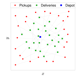
(a) Spatial precedence definition

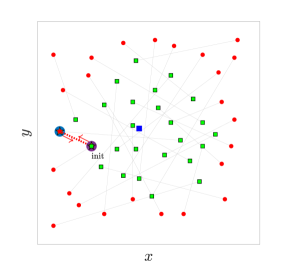
(b) First insertion to a tour initialized at a delivery location

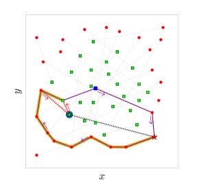
(c) First insertion of a delivery node with valid segment highlighted

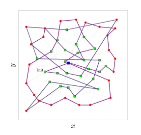
(d) Hamiltonian tour that was initialized at the delivery location

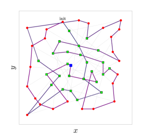
(e) Best Hamiltonian tour that was initialized at a pickup location

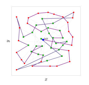
(f) Hamiltonian tour when initialized at the depot location

Figure 1: Illustrative example of the adapted CIH algorithm on a problem with 25 pickup and delivery locations

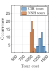
(a) $Q=2$ items

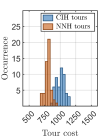
(b) $Q=4$ items

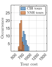
(c) $Q=6$ items

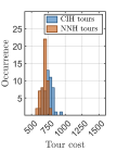
(d) $Q=8$ items

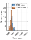
(e) $Q=10$ items

Figure 2: Histograms of tour costs obtained by initiating the tours at each location of the m-PDTSP point cloud.

Consider the example point cloud set of 25 pickup and delivery locations as shown in Fig. 1a, which form $\mathcal{V}_{P}$ and $\mathcal{V}_{D}$ respectively. Their precedence constraints are illustrated using grey line segments and define material handling tasks of moving items from the pickup positions to their respective delivery locations. The objective of the material handling agent is to minimize the total Euclidean distance of the tour, starting and ending its m-PDTSP tour at the depot, marked in blue. For simplicity, the mass of every commodity is identical, and the capacitated agent is capable of carrying the mass of 10 commodities at a time.

First, the construction of the CIH tour is illustrated. The case where the tour is initialized at a delivery location is shown in Fig. 1b. The first feasible insertion is highlighted in blue, as obtained using algorithm 2 and the construction phase of the tour at this instance is highlighted, showing a pickup being added. Points with the lowest insertion cost ratios are inserted into the tour to construct the CIH tour. The first instance when a delivery node is inserted is shown in Fig. 1c. The valid partition of the tour where it can be inserted is highlighted and is the segment that has already visited the associated pickup, and for the entire tour, cargo constraints are not violated by the insertion. The complete tour, as obtained after initializing at the original delivery location (marked) is shown in Fig. 1d. It can be verified that all nodes are visited while maintaining precedence and cargo constraints. When initializing at a pickup location, the completed tour obtained using the proposed CIH algorithm is shown in Fig. 1e, while Fig. 1f shows the same when initialized at the depot.

It is worth noting the significant difference in tours of Fig. 1d, 1e and 1f, showcasing the advantage of considering various initialization locations and adjusting the payload initialization to maintain feasibility. For various cargo capacities, Fig. 2 shows the variation of tour costs obtained due to the initialization at every location of the point cloud. The dependence of tour cost on cargo capacity $Q$ is immediately apparent.

Next, the NNH tour generation is discussed for the same example. Consider the case where the tour is initialized at the marked delivery location of Fig. 3a, where the resulting tour after 2 concatenations is shown. At the next instance, the feasible next locations are marked with dotted lines, after considering the payload and precedence constraints of the existing tour. The star-marked location is the closest feasible location and is thus added to the tour, extending the tour by 1 location. This is repeated until all the points have been inserted, resulting in the complete tour shown in Fig. 3b. In this manner, the NNH algorithm efficiently and rapidly finds feasible tours.

The best tour obtained when initialized with pickup locations is shown in Fig. 3c while the tour obtained when initialized with the depot is shown in Fig. 3d. Significant variation can be seen in the tours, each of which respects precedence and cargo constraints. As described in algorithm 1, NNH tours are initiated at every location of the point cloud and the minimum tour cost is selected as the NNH tour.

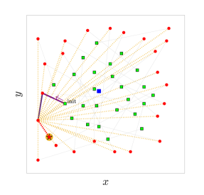
(a) Feasible points for insertion after 2 insertions, and selected point

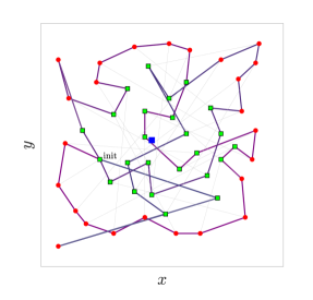
(b) Fully constructed Hamiltonian tour, initialized at a delivery node

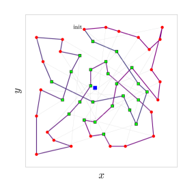
(c) Best Hamiltonian tour that was initialized at a pickup node

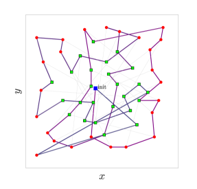
(d) Hamiltonian tour, initialized at the depot

Figure 3: Illustrative example of the adapted CIH algorithm for the non-Euclidean TSP-PC instance with 51 points

VI Computational Experiments

Considering the added algorithmic complexity of the CIH, it was expected that it would perform better than the NNH, as described in TSP literature [33, 39]. However, this was not the case seen in Fig. 2. Computational experiments are systematically conducted to verify this finding across a variety of test cases, varying the spatial relations of the precedence constraints and the cargo capacity $Q$ of the material handling agent.

To compare the ability of the CIH and NNH algorithms to rapidly generate good solutions across a variety of test cases, sufficiently diverse benchmark instances that enable the analysis of the effect of spatial precedence constraints are not readily available for the m-PDTSP. For this reason, the popular TSPLIB benchmark instances [37] are modified in a reproducible manner to add precedence constraints as detailed below.

1. Load a TSPLIB point cloud that has 2D Cartesian coordinates defined for every point. Let $n$ be the number of points.

2. Find the centroid of the point cloud.

3. Sort and assign indices to the points by order of increasing distance from the centroid. Let the indices be $1,2,...,n$ for the sorted points.

4. Designate the point with index 1 as the depot.

5. Define precedence constraints between points with pairs of indices as $(2\prec n),(3\prec n-1),(4\prec n-2)$ and so on.

The described method instantiates cases where the pickup nodes are closer to the depot, which is closest to the centroid. In fact, Fig. 1a is an example of such a modification applied to the ‘eil51’ instance of the TSPLIB. The complementary case where the delivery nodes are to be spatially closer to the centroid is also studied, where the direction of the precedence constraints in Step 2 are reversed. Finally, for each modified case with added precedence constraints, the agent’s cargo capacity $Q$ is also varied, enabling it to carry a certain maximum number of commodities, to account for the effect of cargo capacity on the heuristic performance.

(a) Histogram of the ratio of NNH cost to CIH cost when delivery nodes are centrally located

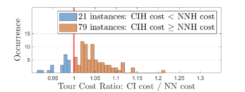
(b) Histogram of the ratio of NNH cost to CIH cost when pickup nodes are centrally located

Figure 4: Performance comparison of the CIH and NNH algorithms for varying spatial precedence constraints.

The ratio of tour cost obtained using CIH to that obtained using NNH is shown in Fig. 4, differentiated by the spatial nature of the precedence constraints. As seen in the histogram of Fig. 4a, the NNH tour cost was lower than the CIH case in 98% of the instances studied, resulting in up to 30% reduction in the tour cost in some instances. It is clear that the performance of the CIH algorithm is dependent on the proximity of the delivery nodes to the depot, as seen by the improvement in Fig. 4b, corresponding well with the observations in [36]. Regardless, the NNH still outperforms the CIH in $>$ 88% of the overall cases studied when accounting for both types of spatial precedence constraints.

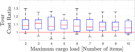
(a) Box plot of tour cost ratio between the CIH and NNH tours, for various cargo capacities

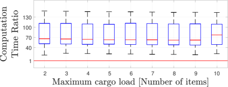
(b) Box plot of computation time ratio between the CIH and NNH algorithms, for various cargo capacities

Figure 5: Effect of maximum cargo capacity on the performance of the NNH and CIH algorithms

The effect of cargo capacity is isolated in Fig. 5 and shows no significant effect on the relative performance of the two heuristics. Worth noting is that no performance gain is provided by the CIH, despite the increased computation time. Finally, the effect of the number of overall locations on the two heuristics is shown in Fig. 6. As expected, the algorithmic complexity of the CIH algorithm results in increased effort as the number of locations is increased. The actual computation time taken by the two heuristics on an Intel Core i7-9750H CPU are shown in Fig. 7, where it is seen that the NNH provides near instantaneous solutions, unlike the CIH.

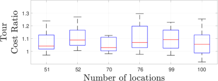
(a) Histogram of the tour cost ratio between the CIH solution and NN solution

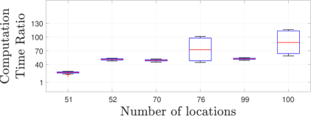
(b) Histogram of the tour cost ratio between the CIH solution and NN solution

Figure 6: Effect of number of locations on the performance of the NNH and CIH algorithms

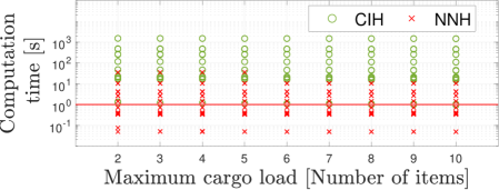
Figure 7: Point cloud of computation time of the two algorithms

VII Conclusion

The well-known Cheapest Insertion Heuristic and Nearest Neighbor Heuristics have been extended to systematically account for the precedence and cargo constraints of the m-PDTSP. The presented algorithms further enable the generation of multiple feasible tours by initializing the heuristic at every location, regardless of its classification as a pickup, delivery or depot node.

A systematic study was conducted to evaluate the algorithm performance, isolating the effects of constraints and problem size. When compared to the CIH algorithm, in a majority of cases, the NNH almost instantaneously provides better tours regardless of the number of points, cargo capacity or precedence constraints. While there is some correlation between the spatial nature of precedence constraints and the performance of the CIH algorithm, it is not significant, and the NNH algorithm is clearly better suited to the m-PDTSP problem. Thus, depending on the use-case and time available, it may be worthwhile to compute the CIH tour in addition to the NNH tour and simply choose the tour with minimum cost between the two.

Future work will focus on implementing the NNH heuristic in the context of instantaneous online rescheduling of a fleet of material handling agents when system parameters vary in real-time. Considering the ability of the heuristic to rapidly generate multiple feasible solutions, it is well suited to evolutionary or population-based metaheuristic algorithms. The solution set obtained from the NNH heuristic can also replace rollout algorithms within a reinforcement learning framework. The heuristic will further be extended to consider battery capacity limitations and charging time for battery-powered agents.

References

- [1] L. F. Escudero, “An inexact algorithm for the sequential ordering problem,” European Journal of Operational Research, vol. 37, no. 2, pp. 236–249, 1988.
- [2] L. F. Escudero, M. Guignard, and K. Malik, “A lagrangian relax-and-cut approach for the sequential ordering problem with precedence relationships,” Annals of Operations Research, vol. 50, no. 1, pp. 219–237, 1994.
- [3] N. Ascheuer, “Hamiltonian path problems in the on-line optimization of flexible manufacturing systems,” Ph.D. dissertation, 1996.
- [4] N. Ascheuer, L. F. Escudero, M. Grötschel, and M. Stoer, “A cutting plane approach to the sequential ordering problem (with applications to job scheduling in manufacturing),” SIAM Journal on Optimization, vol. 3, no. 1, pp. 25–42, 1993.
- [5] S. Spieckermann, K. Gutenschwager, and S. Voß, “A sequential ordering problem in automotive paint shops,” International journal of production research, vol. 42, no. 9, pp. 1865–1878, 2004.
- [6] M. T. Fiala Timlin and W. R. Pulleyblank, “Precedence constrained routing and helicopter scheduling: heuristic design,” Interfaces, vol. 22, no. 3, pp. 100–111, 1992.
- [7] S. Anily and J. Bramel, “Approximation algorithms for the capacitated traveling salesman problem with pickups and deliveries,” Naval Research Logistics (NRL), vol. 46, no. 6, pp. 654–670, 1999.
- [8] H. Hernández-Pérez and J.-J. Salazar-González, “The multi-commodity one-to-one pickup-and-delivery traveling salesman problem,” European Journal of Operational Research, vol. 196, no. 3, pp. 987–995, 2009.
- [9] C. Holland, J. Levis, R. Nuggehalli, B. Santilli, and J. Winters, “Ups optimizes delivery routes,” Interfaces, vol. 47, no. 1, pp. 8–23, 2017.
- [10] Z. Ghelichi and S. Kilaru, “Analytical models for collaborative autonomous mobile robot solutions in fulfillment centers,” Applied Mathematical Modelling, vol. 91, pp. 438–457, 3 2021.
- [11] R. Yan, L. Jackson, and S. Dunnett, “A study for further exploring the advantages of using multi-load automated guided vehicles,” Journal of Manufacturing Systems, vol. 57, pp. 19–30, 10 2020.
- [12] J. Morgan, M. Halton, Y. Qiao, and J. G. Breslin, “Industry 4.0 smart reconfigurable manufacturing machines,” pp. 481–506, 4 2021.
- [13] M. G. Mehrabi, A. G. Ulsoy, and Y. Koren, “Reconfigurable manufacturing systems: Key to future manufacturing,” Journal of Intelligent Manufacturing, vol. 11, pp. 403–419, 2000.
- [14] I. Rodríguez-Martín and J. José Salazar-González, “A hybrid heuristic approach for the multi-commodity one-to-one pickup-and-delivery traveling salesman problem,” Journal of Heuristics, vol. 18, pp. 849–867, 2012.
- [15] H. Hernández-Pérez, J. J. Salazar-González, and B. Santos-Hernández, “Heuristic algorithm for the split-demand one-commodity pickup-and-delivery travelling salesman problem,” Computers & Operations Research, vol. 97, pp. 1–17, 2018.
- [16] H. Hernández-Pérez and J.-J. Salazar-González, “A branch-and-cut algorithm for a traveling salesman problem with pickup and delivery,” Discrete Applied Mathematics, vol. 145, no. 1, pp. 126–139, 2004.
- [17] J. Jamal, G. Shobaki, V. Papapanagiotou, L. M. Gambardella, and R. Montemanni, “Solving the sequential ordering problem using branch and bound,” in 2017 IEEE Symposium Series on Computational Intelligence (SSCI). IEEE, 2017, pp. 1–9.
- [18] G. Shobaki and J. Jamal, “An exact algorithm for the sequential ordering problem and its application to switching energy minimization in compilers,” Computational Optimization and Applications, vol. 61, no. 2, pp. 343–372, 2015.
- [19] Y. Salii, “Revisiting dynamic programming for precedence-constrained traveling salesman problem and its time-dependent generalization,” European Journal of Operational Research, vol. 272, no. 1, pp. 32–42, 2019.
- [20] Z. Xiang, C. Chu, and H. Chen, “The study of a dynamic dial-a-ride problem under time-dependent and stochastic environments,” European Journal of Operational Research, vol. 185, no. 2, pp. 534–551, 2008.
- [21] K.-I. Wong, A. Han, and C. Yuen, “On dynamic demand responsive transport services with degree of dynamism,” Transportmetrica A: Transport Science, vol. 10, no. 1, pp. 55–73, 2014.
- [22] N. Marković, R. Nair, P. Schonfeld, E. Miller-Hooks, and M. Mohebbi, “Optimizing dial-a-ride services in maryland: benefits of computerized routing and scheduling,” Transportation Research Part C: Emerging Technologies, vol. 55, pp. 156–165, 2015.
- [23] K. Braekers, A. Caris, and G. K. Janssens, “Exact and meta-heuristic approach for a general heterogeneous dial-a-ride problem with multiple depots,” Transportation Research Part B: Methodological, vol. 67, pp. 166–186, 2014.
- [24] M. A. Masmoudi, M. Hosny, K. Braekers, and A. Dammak, “Three effective metaheuristics to solve the multi-depot multi-trip heterogeneous dial-a-ride problem,” Transportation Research Part E: Logistics and Transportation Review, vol. 96, pp. 60–80, 2016.
- [25] T. Baltussen, M. Goutham, M. Menon, S. Garrow, M. Santillo, and S. Stockar, “A parallel monte-carlo tree search-based metaheuristic for optimal fleet composition considering vehicle routing using branch & bound,” arXiv preprint arXiv:2303.03156, 2023.
- [26] M. Charikar, R. Motwani, P. Raghavan, and C. Silverstein, “Constrained tsp and low-power computing,” in Workshop on Algorithms and Data Structures. Springer, 1997, pp. 104–115.
- [27] A. Grigoryev and O. Tashlykov, “Solving a routing optimization of works in radiation fields with using a supercomputer,” in AIP Conference Proceedings, vol. 2015, no. 1. AIP Publishing LLC, 2018, p. 020028.
- [28] X. Bai, M. Cao, W. Yan, S. S. Ge, and X. Zhang, “Efficient heuristic algorithms for single-vehicle task planning with precedence constraints,” IEEE Transactions on Cybernetics, vol. 51, no. 12, pp. 6274–6283, 2020.
- [29] T. S. Kumar, M. Cirillo, and S. Koenig, “On the traveling salesman problem with simple temporal constraints,” in Tenth Symposium of Abstraction, Reformulation, and Approximation, 2013.
- [30] E. Nunes, M. McIntire, and M. Gini, “Decentralized allocation of tasks with temporal and precedence constraints to a team of robots,” in 2016 IEEE International Conference on Simulation, Modeling, and Programming for Autonomous Robots (SIMPAR). IEEE, 2016, pp. 197–202.
- [31] S. Edelkamp, M. Lahijanian, D. Magazzeni, and E. Plaku, “Integrating temporal reasoning and sampling-based motion planning for multigoal problems with dynamics and time windows,” IEEE Robotics and Automation Letters, vol. 3, no. 4, pp. 3473–3480, 2018.
- [32] T. Nicholson, “A sequential method for discrete optimization problems and its application to the assignment, travelling salesman, and three machine scheduling problems,” IMA Journal of Applied Mathematics, vol. 3, no. 4, pp. 362–375, 1967.
- [33] D. J. Rosenkrantz, R. E. Stearns, and P. M. Lewis, II, “An analysis of several heuristics for the traveling salesman problem,” SIAM journal on computing, vol. 6, no. 3, pp. 563–581, 1977.
- [34] G. Reinelt, The traveling salesman: computational solutions for TSP applications. Springer, 2003, vol. 840.
- [35] L. Ivanova, A. Kurkin, and S. Ivanov, “Methods for optimizing routes in digital logistics,” in E3S Web of Conferences, vol. 258. EDP Sciences, 2021, p. 02015.
- [36] M. Goutham, M. Menon, S. Garrow, and S. Stockar, “A convex hull cheapest insertion heuristic for the non-euclidean and precedence constrained tsps,” arXiv e-prints, pp. arXiv–2302, 2023.
- [37] G. Reinhelt, “TSPLIB: a library of sample instances for the tsp (and related problems) from various sources and of various types,” URL: http://comopt.ifi.uni-heidelberg.de/software/TSPLIB95/, 2014.
- [38] M. F. Dacey, “Selection of an initial solution for the traveling-salesman problem,” Operations Research, vol. 8, no. 1, pp. 133–134, 1960.
- [39] G. W. DePuy, R. J. Moraga, and G. E. Whitehouse, “Meta-raps: a simple and effective approach for solving the traveling salesman problem,” Transportation Research Part E: Logistics and Transportation Review, vol. 41, no. 2, pp. 115–130, 2005.