Simulation-based, Finite-sample Inference for Privatized Data

Abstract

Privacy protection methods, such as differentially private mechanisms, introduce noise into resulting statistics which often results in complex and intractable sampling distributions. In this paper, we propose to use the simulation-based “repro sample” approach to produce statistically valid confidence intervals and hypothesis tests based on privatized statistics. We show that this methodology is applicable to a wide variety of private inference problems, appropriately accounts for biases introduced by privacy mechanisms (such as by clamping), and improves over other state-of-the-art inference methods such as the parametric bootstrap in terms of the coverage and type I error of the private inference. We also develop significant improvements and extensions for the repro sample methodology for general models (not necessarily related to privacy), including 1) modifying the procedure to ensure guaranteed coverage and type I errors, even accounting for Monte Carlo error, and 2) proposing efficient numerical algorithms to implement the confidence intervals and $p$-values.

Keywords: Indirect Inference, Confidence Interval, Hypothesis Test, Differential Privacy

1 Introduction

There is a growing interest in developing privacy-preserving methodologies, and differential privacy (DP) has arisen as the state-of-the-art in privacy protection (Dwork et al., 2006). However, when formal privacy protection methods are applied to sensitive data, the published quantities may have a very different structure/distribution than the original data, which depends on the privatization algorithm. A major benefit of differential privacy is that the privacy mechanism – the noise-adding distribution – can be publicly communicated without compromising privacy. Thus, a statistician or data analyst can, in principle, incorporate the uncertainty due to the privacy mechanism into their statistical reasoning. Despite this potential, there is a need for general-purpose methods to conduct valid statistical inferences on privatized data. A major challenge is that, given a model $\underline{x}\sim f(\underline{x}\mid\theta)$ for the sensitive data and the privacy mechanism $s|\underline{x}\sim\eta(s\mid\underline{x})$, the marginal likelihood function for $\theta$ based on $s$,

$$L(\theta\mid s)=\int_{\underline{x}}f(\underline{x}\mid\theta)\eta(s\mid\underline{x})\ d\underline{x},$$

is often computationally intractable, requiring integration over all possible databases $\underline{x}$. Recently, there have arisen Markov chain Monte Carlo methods to sample from the posterior distribution $\pi(\theta\mid s)$ (Bernstein and Sheldon, 2018, 2019; Kulkarni et al., 2021; Ju et al., 2022), with Ju et al. (2022) giving a general-purpose technique for Bayesian inference on privatized data. However, there are not as many general-purpose frequentist methods. Due to the intractability of the marginal likelihood, most common approaches use approximations, such as the parametric bootstrap (Ferrando et al., 2022) or limit theorems (Wang et al., 2018).

Unfortunately, while these approximate techniques are often reliable in non-private settings, they often do not have finite sample guarantees and may give unacceptable accuracy when applied to privatized data. For example, while the noise for privacy is often asymptotically negligible compared to the statistical estimation rate, researchers have found that arguments based on convergence in distribution often result in unsatisfactory approximations (Wang et al., 2018), resulting in unreliable inference. While alternative asymptotic regimes have been proposed (e.g., Wang et al., 2018), they are limited to specific models, mechanisms, and test statistics. Ferrando et al. (2022) proposed using the parametric bootstrap on privatized data, but in order to prove the consistency of their method, they assumed that the data was not clamped, while clamping is often necessary in DP mechanisms. Thus, as we will demonstrate in this paper, the parametric bootstrap often gives unacceptable accuracy on privatized data.

While the marginal likelihood may not be easily evaluated, it is often the case that both $f(\underline{x}\mid\theta)$ and $\eta(s\mid\underline{x})$ are relatively easy to sample from. This aspect makes simulation-based inference a good candidate for analyzing privatized data. Our simulation-based (also known as indirect inference) framework is inspired by the “repro samples” framework of Xie and Wang (2022), and the general setup is similar to other simulation-based works as well (Guerrier et al., 2019), and is widely applicable to statistical problems, beyond DP.

We assume that rather than directly sampling from our model/mechanism, given a parameter $\theta$, we can separately sample a “seed” $u$ from a known distribution $P$ (not involving $\theta$), and apply a function that combines the seed and the parameter to produce the observed random variable: $s=G(\theta,u)$. Intuitively, $s=G(\theta,u)$ can be thought of as the equation that generated the observed $s$, where $u$ is the source of randomness. Since the true parameter is unknown, in simulation-based inference, we simulate seeds $\{u_{i}\}_{i=1}^{R}$ from $P$ and hold these fixed during our search over the parameter space for the parameter(s) $\hat{\theta}$ that make the values $G(\hat{\theta},u_{1}),\ldots,G(\hat{\theta},u_{R})$ “similar” to our observed $s$, where ideally a higher similarity measure will result in better estimates $\hat{\theta}$ of $\theta$. While determining the distribution $P$ and the mapping $G$ are problem-specific, this decomposition can be derived for many models and privacy mechanisms.

The “repro sample” approach of Xie and Wang (2022) uses the above framework to construct confidence sets, offering great flexibility, especially in smaller sample sizes and unusual models. They prove that their abstract confidence sets have guaranteed coverage, but their implementations may have inaccuracies due to the Monte Carlo errors. Furthermore, their Monte Carlo method for obtaining the confidence interval requires an inefficient grid search over the parameter space.

Our Contributions In this paper, we propose applying the simulation-based inference approach to privatized data, resulting in the following contributions:

• We use our methodology to tackle several DP inference problems, giving provable inference guarantees and improving over state-of-the-art methods (such as the parametric bootstrap.)

• We demonstrate that our methodology can account for biases introduced by DP mechanisms, such as due to clamping or other non-linear transformations.

Motivated by the need for statistically valid inference on privatized data, we also improved and expanded the repro samples methodology.

• We modify the repro samples method to ensure guaranteed coverage and type I errors, even accounting for Monte Carlo errors, and present the repro methodology with a new notation to better communicate the applicability of the framework.

• We propose computationally efficient algorithms for computing valid $p$-values and confidence intervals.

Finally, we point out that while our methodology is motivated by problems in privacy, our framework is actually very general and can be applied to non-DP settings as well. Our approach is particularly applicable when one has a low dimensional summary statistic but may not even have an estimator for the true parameters, let alone an understanding of the sampling distribution.

Organization The remainder of the paper is organized as follows: In Section 2 we set the notation for the paper and review some necessary background on differential privacy. In Section 3, we start by giving an abstract framework for generating confidence sets in Section 3.1, use this to develop simulation-based confidence sets in Section 3.2 with guaranteed coverage, and develop a numerical algorithm for simulation-based confidence intervals in Section 3.3. In Section 4, we review how repro samples can be used to test hypotheses, and give a clear formula for a valid $p$-value, as well as an efficient numerical algorithm. In Section 5, we conduct several simulation studies, applying our methodology to various DP inference problems. We conclude in Section 6 with some discussion and directions for future work. In Section 6.1, we spend some extra time discussing the choice of the test statistic in the repro methodology, and quantify the cost of over-coverage, which is common when using the repro methodology. While our methodology is based on the repro sample framework of Xie and Wang (2022), all of our results and proofs are self-contained. Proofs as well as technical lemmas and simulation details are deferred to the supplement.

Related work The area of indirect inference was proposed by Gourieroux et al. (1993), which initially gave a simulation-based approach to bias correction and parameter estimation. However, the inferential method proposed by Gourieroux et al. (1993) is based on large sample theory, which is often unreliable in privacy problems. Guerrier et al. (2019, 2020); Zhang et al. (2022) developed a more theoretical basis for the indirect inference approach, focusing on bias-correction. Xie and Wang (2022) developed the repro sample methodology, which is the basis for the simulation-based inference techniques proposed in this paper. Wang et al. (2022) applied the repro sample methodology to develop model and coefficient inference in high-dimensional linear regression.

In the area of statistical inference on privatized data, there are several notable works. For Bayesian inference on privatized data, Ju et al. (2022) proposed a general Metropolis-within-Gibbs algorithm, which correctly targets the posterior distribution. In the frequentist setting, Wang et al. (2018) developed a custom asymptotic framework that ensures, under certain circumstances, that the approximations produced are at least as accurate as similar approximations for the non-private data. While lacking finite-sample guarantees, Ferrando et al. (2022) showed that the parametric bootstrap is a very flexible technique to perform inference on privatized data.

There have also been several works that tailor their statistical inference to particular models and mechanisms. Awan and Slavković (2018) developed uniformly most powerful DP tests for Bernoulli data, and Awan and Slavković (2020) extended this work to produce optimal confidence intervals as well. Drechsler et al. (2022) developed private non-parametric confidence intervals for the median. Karwa and Vadhan (2018) developed private confidence intervals for the mean of normally distributed data. Covington et al. (2021) developed a DP mechanism to generate confidence intervals for general parameter estimation, based on the CoinPress algorithm (Biswas et al., 2020) and the bag of little bootstraps (Kleiner et al., 2012).

In contrast with many of the related works above, the goal of this paper is to produce valid finite-sample frequentist inference for a wide variety of models and mechanisms. In particular, we will not ask that the privacy mechanism be tailored for our model or for our particular statistical task. While Ju et al. (2022) offered a general solution in the Bayesian setting, there are essentially no frequentist techniques to derive valid finite-sample inference for general models and mechanisms.

2 Background

In this section, we review the necessary background and set the notation for the paper.

We call a function $T:\mathscr{X}\times\mathscr{X}^{n}\rightarrow\mathscr{Y}$ permutation-invariant if for any permutation $\pi$ on $\{1,2,\ldots,n\}$, we have $T(x;(x_{i})_{i=1}^{n})=T(x;(x_{\pi(i)})_{i=1}^{n})$. Note that if $X_{1},\ldots,X_{n}$ are exchangeable random variables in $\mathscr{X}$, and $T$ is a permutation-invariant function, then the sequence of random variables, $T(X_{1};(X_{i})_{i=1}^{n}),T(X_{2};(X_{i})_{i=1}^{n}),\ldots,T(X_{n};(X_{i})_{i=1}^{n})$ is also exchangeable.

For a real value $x$, we define $\lfloor x\rfloor$ to be the greatest integer less than or equal to $x$, and $\lceil x\rceil$ to be the smallest integer greater than or equal to $x$. We define the clamp function $[\cdot]_{a}^{b}:\mathbb{R}\rightarrow[a,b]$ as $[x]_{a}^{b}=\min\{\max\{x,a\},b\}$. Many differentially private mechanisms use clamping to ensure finite sensitivity; see Example 2.4.

In this paper, we will use $s$ to denote the observed “sample.” While in many statistical problems, a sample consists of i.i.d. data, in this paper, we allow $s$ to generally be the set of observed random variables from an experiment. In differential privacy, the observed values after privatization are often low-dimensional quantities. We will use superscripts such as $s^{(j)}$ to denote the $j^{th}$ entry of $s$, and subscripts $s_{i}$ to denote the $i^{th}$ element of a list $s_{1},\ldots,s_{R}$.

Example 2.1 (Bernoulli example).

One of the simplest models is independent Bernoulli data. Suppose that $x_{i}\overset{\text{iid}}{\sim}\mathrm{Bern}(\theta)$, and $(x_{1},x_{2},\ldots,x_{n})$ represents a confidential dataset. If we are interested in doing inference on $\theta$, the total $X=\sum_{i=1}^{n}x_{i}$ is a sufficient statistic, but for privacy purposes, we will instead base our inference solely on $\tilde{X}=X+N$, where $N$ is a random variable independent of $X$ chosen such that $\tilde{X}$ satisfies differential privacy (Vu and Slavkovic, 2009; Awan and Slavković, 2018). In this paper, we consider our “sample” to be the observed value $s\vcentcolon=\tilde{X}$.

2.1 Differential privacy

Differential privacy, introduced by Dwork et al. (2006), is a probabilistic framework used to quantify the privacy loss of a mechanism (randomized algorithm). In the big picture, differential privacy requires that for any two neighboring databases – differing in one person’s data, the resulting distributions of outputs are “close”. There have been many variants of differential privacy proposed, which alter both the notion of “neighboring” as well as ”close”. Typically, the neighboring relation is expressed in terms of an adjacency metric on the space of input databases, and the closeness measure is formulated in terms of a divergence or constraints on hypothesis tests.

If $\mathscr{D}$ is the space of input datasets, a metric $d:\mathscr{D}\times\mathscr{D}\rightarrow\mathbb{R}^{\geq 0}$ is an adjacency metric if $d(D,D^{\prime})\leq 1$ represents that $D$ and $D^{\prime}$ differ by one individual. When $d(D,D^{\prime})\leq 1$, we say that $D$ and $D^{\prime}$ are neighboring or adjacent datasets. A mechanism $M:\mathscr{D}\rightarrow\mathscr{Y}$ is a randomized algorithm; more formally, for each $D\in\mathscr{D}$, $M(D)|D$ is a random variable taking values in $\mathscr{Y}$.

Definition 2.2 (Differential privacy: Dwork et al. (2006)).

Let $\varepsilon\geq 0$, let $d$ be an adjacency metric on $\mathscr{D}$, and let $M:\mathscr{D}\rightarrow\mathscr{Y}$ be a mechanism. We say that $M$ satisfies $\varepsilon$-differential privacy ($\varepsilon$-DP) if $P(M(D)\in S)\leq\exp(\varepsilon)P(M(D^{\prime})\in S)$, for all $d(D,D^{\prime})\leq 1$ and all measurable sets $S\subset\mathscr{Y}$.

In many problems, the space of datasets can be expressed as $\mathscr{D}=\mathscr{X}^{n}$, where $\mathscr{X}$ represents the space of possible contributions from one individual and $n$ is fixed. In this case, it is common to take the adjacency metric to be Hamming distance, which counts the number of different entries between two databases. This setup is commonly referred to bounded DP. The inference framework proposed in this paper is applicable to general database spaces and metrics, but the examples will focus on bounded DP for simplicity.

Another common formulation of DP is Gaussian-DP, where the measure of “closeness” is expressed in terms of hypothesis tests.

Definition 2.3 (Gaussian DP: Dong et al., 2022).

Let $\mu\geq 0$, let $d$ be an adjacency metric on $\mathscr{D}$, and let $M:\mathscr{D}\rightarrow\mathscr{Y}$ be a mechanism. We say that $M$ satisfies $\mu$-Gaussian DP ($\mu$-GDP) if for any two adjacent databases $D$ and $D^{\prime}$ satisfying $d(D,D^{\prime})\leq 1$, the type II error of any hypothesis test on $H_{0}:Z\sim M(D)$ versus $H_{1}:Z\sim M(D^{\prime})$, where $Z$ is the observed output of $M$, is no smaller than $\Phi(\Phi^{-1}(1-\alpha)-\mu),$ where $\alpha$ is the type I error, and $\Phi$ is the cumulative distribution function (cdf) of a standard normal random variable.

One can interpret GDP as follows: a mechanism satisfies $\mu$-GDP if testing $H_{0}:Z\sim M(D)$ versus $H_{1}:Z\sim M(D^{\prime})$ for adjacent databases is at least as hard as testing $H_{0}:Z\sim N(0,1)$ versus $H_{1}:Z\sim N(\mu,1)$.

Differential privacy satisfies basic properties such as composition and post-processing:

• Composition: if a mechanism $M_{1}:\mathscr{D}\rightarrow\mathscr{Y}$ satisfies $\varepsilon_{1}$-DP ($\mu_{1}$-GDP) and mechanism $M_{2}:\mathscr{D}\rightarrow\mathscr{Z}$ satisfies $\varepsilon_{2}$-DP ($\mu_{2}$-GDP), then the composed mechanism which releases both $M_{1}(D)$ and $M_{2}(D)$ satisfies $(\varepsilon_{1}+\varepsilon_{2})$-DP ($\sqrt{\mu_{1}^{2}+\mu_{2}^{2}}$-GDP).

• Post-processing: if a mechanism $M:\mathscr{D}\rightarrow\mathscr{Y}$ satisfies $\varepsilon$-DP ($\mu$-GDP) and $f:\mathscr{Y}\rightarrow\mathscr{Z}$ is another mechanism, then $f\circ M:\mathscr{D}\rightarrow\mathscr{Z}$ satisfies $\varepsilon$-DP ($\mu$-GDP).

Example 2.4 (Additive noise mechanism).

Given a statistic $T:\mathscr{D}\rightarrow\mathbb{R}^{d}$, and a norm $\lVert\cdot\rVert$ on $\mathbb{R}^{d}$, an additive noise mechanism samples a random vector $N$ independent of the dataset, and releases $\widetilde{T}(D)=T(D)+\Delta N$, where $\Delta=\sup_{d(D,D)\leq 1}\lVert T(D)-T(D^{\prime})\rVert$ is the sensitivity of $T$. The Laplace mechanism uses the $\ell_{1}$ norm and samples $N_{i}\overset{\text{iid}}{\sim}\mathrm{Laplace}(0,1/\varepsilon)$ for $i=1,\ldots,d$; then $\widetilde{T}(D)$ satisfies $\varepsilon$-DP. The Gaussian mechanism uses the $\ell_{2}$ norm and samples $N\sim N_{d}(0,(1/\mu^{2})I)$ and $\widetilde{T}(D)$ satisfies $\mu$-GDP.

Given a real-valued statistic of the form $T(D)=\frac{1}{n}\sum_{i=1}^{n}t(x_{i})$, where $D=(x_{1},\ldots,x_{n})$, many DP mechanisms will often first alter $T$ using a clamp function, to ensure finite sensitivity: $T^{\prime}(D)=\frac{1}{n}\sum_{i=1}^{n}[t(x_{i})]_{a}^{b}$, and then apply an additive noise mechanism to $T^{\prime}(D)$. However, clamping is a non-linear function, which results in bias.

3 Confidence intervals

Confidence intervals are a fundamental statistical tool, which concretely communicates the uncertainty of a parameter estimate. In Section 3.1, we describe a general and abstract framework for constructing a confidence set, which encompasses both traditional methods as well as the simulation-based method explored in this paper. In Section 3.2, we show that, using simulation-based inference, we can construct valid confidence sets with guaranteed coverage, even accounting for the randomness in the simulation. In Section 3.3, we give a concrete algorithm for implementing the confidence set prescriptions in Section 3.2 under the assumption that the resulting confidence set is an interval.

3.1 Abstract confidence sets

In this section, we set up a general and abstract framework for constructing a confidence set for an unknown parameter $\theta$ where the main result is in Lemma 3.1.

The abstraction in Lemma 3.1 is motivated by the framework in Xie and Wang (2022), but we present our framework using a different notation and perspective. We hope that our presentation offers a clearer interpretation and easier implementation.

Lemma 3.1.

Let $\alpha\in(0,1)$ be given. Let $\theta^{*}\in\Theta$ be the unknown parameter, $s$ be the observed sample where $s\sim F_{\theta^{*}}$, and $u\sim P$ be a random variable independent of $s$, which we call a “seed”. For any fixed $\theta$, let $B_{\alpha}(\theta;s,u)$ be an event, which depends on $s$ and $u$, such that for all $\theta\in\Theta$,

$$P_{s\sim F_{\theta},u\sim P}(B_{\alpha}(\theta;s,u))\geq 1-\alpha.$$ (1)

Then

$$\Gamma_{\alpha}(s,u)\vcentcolon=\{\theta\mid I(B_{\alpha}(\theta;s,u))=1\},$$ (2)

is a $(1-\alpha)$-confidence set for $\theta^{*}$. If $\theta=(\beta,\eta)$ is a decomposition of the parameter, then

$$\Gamma^{\beta}_{\alpha}(s,u)=\{\beta\mid\exists\eta\text{ s.t. }I(B_{\alpha}((\beta,\eta);s,u))=1\},$$ (3)

is a $(1-\alpha)$-confidence set for $\theta$. More generally, if $\theta=(\theta_{1},\ldots,\theta_{k})$, then $\Gamma_{\alpha}^{\theta_{1}}(s,u),\ldots,\Gamma_{\alpha}^{\theta_{k}}(s,u)$ are simulataneous $(1-\alpha)$-confidence sets for $\theta_{1}^{*},\ldots,\theta_{k}^{*}$.

Figure 1: An illustration for $B_{\alpha}(\theta;s,u)$ and $\Gamma_{\alpha}(s,u)$ in Lemma 3.1. The left subfigure is the space of parameter $\theta\in\mathbb{R}^{2}$, and the right subfigure is the space of $s\in\mathbb{R}^{2}$. The true parameter is $\theta^{*}$, and the observed sample is $s^{*}$, where both are denoted by $\bigstar$. For each $\theta$, we can construct $B_{\alpha}(\theta;s,u)$ (e.g., by simulation as in Theorem 3.6: the points in the right subfigure correspond to $\{s_{i}\}_{i=1}^{R}$), and we obtain $\Gamma_{\alpha}(s,u)$ by collecting the $\theta$ such that its corresponding $\{s|I(B_{\alpha}(\theta;s,u))=1\}$ contains $s^{*}$. For example, in the left subfigure, the parameters denoted by the red $+$ and blue $\circ$ are in $\Gamma_{\alpha}(s,u)$ while the one by green $\times$ is not. Note that $\Gamma_{\alpha}(s,u)$ is a valid confidence set with level $1-\alpha$ since for every $\theta\in\Theta$, we have $s\sim F_{\theta}$ being in $\{s|I(B_{\alpha}(\theta;s,u))=1\}$ with probability $1-\alpha$, which means $P(\theta\in\Gamma_{\alpha}(s,u))\geq 1-\alpha$. Furthermore, the confidence set $\Gamma_{\alpha}^{\theta_{1}}(s,u)$ is shown in the left subfigure, illustrating that it is the projection of $\Gamma_{\alpha}(s,u)$ onto the component $\theta_{1}$.

One way of understanding the construction in Lemma 3.1 is as follows: for every candidate value of $\theta$, build an event $B_{\alpha}(\theta;s,u)$ which happens with probability $(1-\alpha)$ over the randomness of $s\sim F_{\theta}$ and $u\sim P$. Then, given an observed pair $(s,u)$, our confidence set is simply the set of $\theta$ values for which $B_{\alpha}(\theta;s,u)$ did in fact happen. See Figure 1 for an illustration.

Remark 3.2.

We remark that the confidence sets $\Gamma_{\alpha}^{\theta_{i}}(s,u)$ can be viewed as a projection of $\Gamma_{\alpha}(s,u)$ onto the dimensions involving $\theta_{i}$, which is shown in the left subfigure in Figure 1. It is because each $\Gamma_{\alpha}^{\theta_{i}}(s,u)$ is implicitly constructed from a $\Gamma_{\alpha}(s,u)$ that we get the simultaneous coverage of $\Gamma_{\alpha}^{\theta_{1}}(s,u),\ldots,\Gamma_{\alpha}^{\theta_{k}}(s,u)$. As we will discuss in Section 6.1, a downside of this construction is that the simultaneous nature of the confidence sets can lead to over-coverage for any one of the $\Gamma_{\alpha}^{\theta_{i}}(s,u)$.

When thinking through many traditional methods of confidence intervals, they can usually be expressed in this way, as demonstrated in Example 3.3.

Example 3.3.

We show how the classical method of deriving a confidence interval for the location parameter of the normal distribution fits into the framework of Lemma 3.1. In this case, we will not need the random variable $u$. Let $s=(x_{1},\ldots,x_{n})$ where $x_{i}\overset{\text{iid}}{\sim}N(\theta^{*},\sigma^{2}_{0})$, where only $\theta^{*}$ is unknown. Then $T_{\theta}(s)=\frac{\overline{x}-\theta}{\sigma_{0}/\sqrt{n}}\sim N(0,1)$ is a pivot where $\overline{x}=\frac{1}{n}\sum_{i=1}^{n}x_{i}$. We then take $C=[-z_{1-\alpha/2},z_{1-\alpha/2}]$, which is a $(1-\alpha)$ prediction interval for $T_{\theta^{*}}(s)$, where $\theta^{*}$ is the true parameter. Then $B_{\alpha}(\theta;s)=\{T_{\theta}(s)\in C\}$, and our confidence set is

$$\Gamma_{\alpha}(s) =\{\theta|I(B_{\alpha}(\theta;s))=1\}$$

$$=\{\theta|T_{\theta}(s)\in[-z_{1-\alpha/2},z_{1-\alpha/2}]\}$$

$$=\left\{\theta\middle|-z_{\alpha/2}\leq\frac{\overline{x}-\theta}{\sigma_{0}/\sqrt{n}}\leq z_{\alpha/2}\right\}$$

$$=\left\{\theta\middle|\overline{x}-\sigma_{0}z_{1-\alpha/2}/\sqrt{n}\leq\theta\leq\overline{x}+\sigma_{0}z_{1-\alpha/2}/\sqrt{n}\right\}$$

$$=[\overline{x}-\sigma_{0}z_{1-\alpha/2}/\sqrt{n},\overline{x}+\sigma_{0}z_{1-\alpha/2}/\sqrt{n}],$$

which is the usual confidence interval for the mean.

Example 3.4 below gives a DP example where the sampling distribution of $s$ can be evaluated numerically. However, in most DP problems, this is not the case. For the remainder of the paper, we will not assume that this sampling distribution is available, and in Section 3.2, we will explain how the auxiliary random variable $u$ allows us to use simulation-based inference to construct an event $B_{\alpha}$ satisfying (1).

Example 3.4 (Bernoulli distribution: Awan and Slavković, 2018).

Awan and Slavković (2018) derived the uniformly most powerful DP hypothesis tests for Bernoulli data and showed that they could be expressed in terms of the test statistic $X+N$, where $X\sim\mathrm{Binomial}(n,p^{*})$ and $N\sim\mathrm{Tulap}(0,b,q)$, where $X$ is based on the privatized data, and the parameters of the Truncated-Uniform-Laplace (Tulap) distribution depend on the privacy parameters $\varepsilon$ and $\delta$. Awan and Slavković (2018) gave a closed-form expression for the cdf of $N$, and showed that the cdf of $X+N$ can be expressed as

$$F_{X+N}(t)=\sum_{x=0}^{n}F_{N}(t-x)F_{X}(x),$$

where $F_{X}$ is the cdf of $X$, and $F_{N}$ is the cdf of $N$. This cdf is then used to derive $p$-values and confidence intervals for $p^{*}$ in Awan and Slavković (2018, 2020).

In the previous example, the convolution of $X$ and $N$ was tractable since there were only two variables, the cdfs of both $X$ and $N$ are easily evaluated, and $X$ took on only a finite number of values. Awan and Vadhan (2021) showed that one could use the inversion of characteristic functions to numerically evaluate the cdf when convolving multiple known distributions, which they applied to the testing of two population proportions. In Section B.1 of the supplement, we show that for exponentially distributed data, we can apply this trick to account for clamping. However, it is not always tractable to evaluate the characteristic function of a clamped random variable.

3.2 Simulation-based confidence intervals

Similar to Xie and Wang (2022), we will use simulation techniques to build the event $B_{\alpha}$ in Section 3.1. Unlike Xie and Wang (2022), our result offers guaranteed coverage, even accounting for the Monte Carlo sampling in the procedure.

We assume that the observed data $s$, drawn from a distribution parametrized by the true parameter $\theta^{*}\in\Theta$, can be expressed as

$$s\overset{d}{=}G(\theta^{*},u),$$ (4)

for a known measurable function $G$ and a random variable $u\sim P$, with known distribution $P$ (not depending on $\theta^{*}$). We will refer to equation (4) as a generating equation, which can be interpreted as the equation that was used to generate the data (Hannig, 2009). We will sometimes refer to $u$ as the “seed” that produced the sample $s$. Generating equations like (4) are used in many areas of statistics, including fiducial statistics (Hannig, 2009), the reparametrization trick in variational autoencoders (Kingma and Welling, 2013), and co-sufficient sampling (Engen and Lillegard, 1997; Lindqvist and Taraldsen, 2005).

Example 3.5.

In a differential privacy setting, it may be more natural to separately model the data and the privacy mechanism as follows: $\underline{x}=(x_{1},\ldots,x_{n})$, $x_{i}\overset{\text{iid}}{\sim}F_{\theta^{*}}$, $s|\underline{x}\sim\eta(\cdot|\underline{x})$, in which case we can specify the function $G$ and the seed $u$ in terms of simpler quantities. Suppose that $x_{i}\overset{d}{=}G_{x}(\theta^{*},u_{i})$, where $u_{i}\sim P_{x}$, and $s|\underline{x}\overset{d}{=}G_{s}(\underline{x},u_{\mathrm{DP}})$, where $u_{\mathrm{DP}}\sim P_{\mathrm{DP}}$. Then, we can write $u=(u_{1},\ldots,u_{n},u_{\mathrm{DP}})$ where $u_{i}\sim P_{x}$ and $u_{\mathrm{DP}}\sim P_{\mathrm{DP}}$ are all independent, giving

$$G(\theta,u)\vcentcolon=G_{s}((G_{x}(\theta,u_{i}))_{i=1}^{n},u_{\mathrm{DP}}),$$

which fits within the framework of (4). For a specific example, see Example 3.9.

The repro sample method then draws $R$ i.i.d. copies $u_{1},\ldots,u_{R}\overset{\text{iid}}{\sim}P$, and for each $\theta\in\Theta$, we consider $s_{i}(\theta)=G(\theta,u_{i})$ for $i=1,\ldots,R$, which are called repro samples. At the true parameter $\theta^{*}$, these Monte Carlo samples $\{s_{i}(\theta^{*})\}_{i=1}^{R}$ have the same distribution as $s$. Then, considering the sequence $s,s_{1}(\theta),\ldots,s_{R}(\theta)$, which consists of the repro samples and the observed sample, we construct the event $B_{\alpha}(\theta;s,(u_{i})_{i=1}^{R})$ such that for every $\theta\in\Theta$, $P_{s\sim F_{\theta},u_{i}\sim P}(B_{\alpha}(\theta;s,(u_{i})_{i=1}^{R}))\geq 1-\alpha$. We then plug in $B_{\alpha}$ into either (2) or (3) to form a valid $(1-\alpha)$-confidence set. We offer a general and constructive method to produce a valid $B_{\alpha}(\theta;s,(u_{i})_{i=1}^{R})$ in Theorem 3.6.

Theorem 3.6.

Let $\alpha\in(0,1)$. Let $s\in\mathscr{X}$ be the observed sample, where $s=G(\theta^{*},u)$, $u\sim P$, and $\theta^{*}$ is the true parameter. Let $u_{1},\ldots,u_{R}\overset{\text{iid}}{\sim}P$, and set $s_{i}(\theta)=G(\theta,u_{i})$ for $i=1,\ldots,R$. Let $T_{\theta}:\mathscr{X}\times\mathscr{X}^{R+1}\rightarrow\mathbb{R}$ be a permutation-invariant function, which serves as a test statistic. Call $T_{\text{obs}}(\theta)=T_{\theta}\big{(}s;s,s_{1}(\theta),\ldots,s_{R}(\theta)\big{)}$, and let $T_{(1)}(\theta),\ldots,T_{(R+1)}(\theta)$ be the order statistics of $T_{\theta}\big{(}s;s,s_{1}(\theta),\ldots,s_{R}(\theta)\big{)},T_{\theta}\big{(}s_{1}(\theta);s,s_{1}(\theta),\ldots,s_{R}(\theta)\big{)},$ $\ldots,T_{\theta}\big{(}s_{R}(\theta);s,s_{1}(\theta),\ldots,s_{R}(\theta)\big{)}$. Then for any $b-a\geq\lceil(1-\alpha)(R+1)\rceil-1$, the event $B_{\alpha}(\theta;s,(u_{i})_{i=1}^{R})=\{T_{\text{obs}}(\theta)\in[T_{(a)}(\theta),T_{(b)}(\theta)]\}$ satisfies (1). Thus, using $B_{\alpha}$ in either (2) or (3) of Lemma 3.1 gives a $(1-\alpha)$-confidence set.

Theorem 3.6 gives a straightforward construction for sets satisfying (1), which, as Lemma 3.1 points out, lead to valid confidence sets. A key difference between these results and those of Xie and Wang (2022) is that our $B_{\alpha}$ sets exactly satisfy (1), even including the Monte Carlo errors. This is in contrast to those proposed in Xie and Wang (2022), which do not account for Monte Carlo errors. The key insights for Theorem 3.6 are 1) the need for a permutation-invariant statistic, 2) the importance of including $s$ on the righthand side of $T$ to ensure exchangeability, and 3) the construction of prediction sets based on order statistics, using reasoning similar to that in conformal prediction (Vovk et al., 2005). See Lemma A.1 in the supplement for details.

Example 3.7.

In this example, we list some examples of permutation-invariant functions, and show how $a$ and $b$ can be chosen for one-sided or two-sided criteria:

1. If $s\in\mathbb{R}$, then setting $T_{\theta}(s;(s_{i}(\theta))_{i=1}^{R})=s$ is trivially permutation-invariant. In this case, both large and small values of $s$ indicate that it is unusual, so we may set $a$ and $(R+1)-b$ to be approximately equal: $a=\lfloor(\alpha/2)(R+1)\rfloor$ and $b=a+\lceil(1-\alpha)(R+1)\rceil-1$.

2. More generally, if $T_{\theta}:\mathscr{X}\rightarrow\mathbb{R}$ is a test statistic, which may also depend on the parameter $\theta$, then this also satisfies the assumptions of Theorem 3.6. If large values indicate that it is unusual, we can set $a=1$ and $b=\lceil(1-\alpha)(R+1)\rceil$. On the other hand, if small values of $T$ indicate that it is unusual, then we set $a=\lfloor\alpha(R+1)\rfloor+1$ and $b=R+1$.

3. In general, most statistical depth functions are permutation-invariant, such as Mahalanobis depth, simplicial depth, and Tukey/Halfspace depth. Typically, depth statistics are designed such that lower depth corresponds to unusual points. For example, Mahalanobis depth is defined as $T(x;X)=[1+(x-\mu_{X})^{\prime}\Sigma_{X}^{-1}(x-\mu_{X})]^{-1}$ where $\mu_{X}$ and $\Sigma_{X}$ are the sample mean and covariance of $X$. To use this depth as the $T$ in Theorem 3.6, we let $X=(s,s_{1}(\theta),\ldots,s_{R}(\theta))$ and $x$ be one of $s,s_{1}(\theta),\ldots,s_{R}(\theta)$, and set $a=\lfloor\alpha(R+1)\rfloor+1$ and $b=R+1$.

Remark 3.8.

We remark that depth statistics were also recommended by Xie and Wang (2022) for use in the repro sampling framework, but they did not account for the Monte Carlo errors as we do in Theorem 3.6.

We end this section with two relatively simple examples, showing how one can apply the repro framework to private inference problems. See Section 5 for additional examples.

Example 3.9 (Poisson Distribution).

Suppose that $\underline{x}=(x_{1},\ldots,x_{n})$, $x_{i}\overset{\text{iid}}{\sim}\mathrm{Pois}(\theta^{*})$, and we observe the privatized statistic $s=\frac{1}{n}\sum_{i=1}^{n}[x_{i}]_{0}^{c}+(c/n)N$, for some noise distribution $N$, where $c$ is a non-negative integer. For this example, we will set $N\sim N(0,1)$, ensuring that $s$ satisfies $1$-GDP.

In this setting, we can set $P_{x}\vcentcolon=\mathrm{Unif}(0,1)$ and sample $u_{i}\sim P_{x}$ for $i=1,\ldots,n$. Then using $G_{x}(\theta,u)=F^{-1}_{\theta}(u)$, where $F^{-1}_{\theta}(\cdot)$ is the quantile function of $\mathrm{Pois}(\theta)$, we have $G_{x}(\theta,u_{i})\overset{\text{iid}}{\sim}\mathrm{Pois}(\theta)$. For the privacy mechanism, we set $P_{\mathrm{DP}}=N(0,1)$ and sample $u_{\mathrm{DP}}\sim N(0,1)$. Using the function $G_{s}(\underline{x},u_{\mathrm{DP}})=\frac{1}{n}\sum_{i=1}^{n}[x_{i}]_{0}^{c}+\frac{c}{n}u_{\mathrm{DP}}$, we have that $s|\underline{x}\overset{d}{=}G_{s}(\underline{x},u_{\mathrm{DP}})$. Then, the full generating equation is, $G(\theta,((u_{i})_{i=1}^{n},u_{\mathrm{DP}}))=\frac{1}{n}\sum_{i=1}^{n}[F^{-1}(u_{i};\theta)]_{0}^{c}+\frac{c}{n}u_{\mathrm{DP}}$.

To generate a simulation-based confidence interval in this setting, we produce $R$ i.i.d. copies of $((u_{i})_{i=1}^{n},u_{\mathrm{DP}})$, and use $a$ and $b$ as specified in Example 3.7 in Theorem 3.6 to form the confidence interval in Lemma 3.1.

Figure 2: $95\%$ confidence set for location-scale normal (Example 3.10, based on $s=(1,0.75)$, generated using $n=100$, $\mu^{*}=1$, $\sigma^{*}=1$, $\epsilon=1$, $U=3$, $L=0$, and $R=200$ repro samples. From left to right: Mahalanobis depth (area 0.41), Halfspace/Tukey depth (area 0.59), Simplicial depth (area 0.52), Spatial depth (area 0.42).

Example 3.10 (Location-scale Normal).

Suppose that $x_{1},\ldots,x_{n}\overset{\text{iid}}{\sim}N(\mu^{*},\sigma^{*})$, and we are interested in a confidence set for $(\mu^{*},\sigma^{*})$. Suppose we are given the clamping bounds $L$ and $U$ so that we work with the clamped data $[x_{i}]_{L}^{U}$. It is easy to see that the clamped mean $\overline{x_{c}}=\frac{1}{n}\sum_{i=1}^{n}[x_{i}]_{L}^{U}$ has sensitivity $\frac{U-L}{n}$, and Du et al. (2020) derived the sensitivity of the sample variance $S^{2}_{c}=\frac{1}{n-1}\sum_{i=1}^{n}([x_{i}]_{L}^{U}-\overline{x_{c}})^{2}$ is $\frac{(U-L)^{2}}{n}$, where the “$c$” subscript reminds us that these statistics are for the clamped data. If $N_{1},N_{2}\overset{\text{iid}}{\sim}N(0,1)$, then a privatized statistic is $s=(s^{(1)},s^{(2)})=(\overline{x}_{c}+\frac{U-L}{n\varepsilon}N_{1},S^{2}_{c}+\frac{(U-L)^{2}}{n\varepsilon}N_{2})$, which satisfies $(\sqrt{2}\varepsilon)$-GDP.

In this example, we have a two-dimensional privatized summary, one for the mean and one for the variance. Since it is non-trivial to construct a well-designed test statistic, we compare different options of statistical depth for use in Theorem 3.6, see Figure 2. See Section 5.2 for details and simulation results. Overall, we recommend the Mahalanobis depth, as it results in the smallest confidence set, is computationally efficient, and avoids ties in the ranking of the depth statistics. Furthermore, there is a connection between Mahalanobis depth and general indirect inference (Gourieroux et al., 1993) since both are based on minimizing the distance from the observed value to the mean over simulated values. Further research may investigate other properties of Mahalanobis depth or other general-purpose summary statistics.

Remark 3.11.

In the special case of Theorem 3.6, where $T_{\theta}=s\in\mathbb{R}$, such as in the Poisson example, one can see that if $G(\theta,u_{i})$ is monotone in $\theta$, and order-preserving (meaning that $\mathrm{rank}(G(\theta,u_{i}))=\mathrm{rank}(u_{i})$), then the confidence sets are guaranteed to be intervals.

On the other hand, when $s\in\mathbb{R}^{d}$, and we are using an arbitrary statistic $T_{\theta}:\mathbb{R}^{d}\times\mathbb{R}^{dn}\rightarrow\mathbb{R}$, one may be concerned whether the confidence set is connected or not. While non-identifiability increases the likelihood of disconnected confidence sets, even for identifiable models, it can be nontrivial to determine whether the constructed confidence set is connected.

3.3 Numerical algorithm for confidence intervals

Algorithm 1 accept($\beta$, $\alpha$, $\Theta=B\times H$, $(u_{i})_{i=1}^{R}$, $G$, $s$, $T$)

INPUT: proposed parameter of interest $\beta\in B$, $\alpha\in[1/(R+1),1)$, decomposition $\Theta=B\times H$ of $\theta=(\beta,\eta)$, seeds $(u_{i})_{i=1}^{R}$, observed statistic $s\in\mathbb{R}^{d}$, exchangeable statistic $T_{\theta}:\mathbb{R}^{d}\times\mathbb{R}^{d(R+1)}\rightarrow[0,1]$, defined for all $\theta\in\Theta$ (low values are interpreted as unusual), and $G(\theta,u)$ is the generating equation for $s$.

 For a given $\theta$, denote $s_{i}(\theta)=G(\theta,u_{i})$.

 Denote $T_{i}(\theta)=T_{\theta}(s_{i}(\theta);s,s_{1}(\theta),\ldots,s_{R}(\theta))$

 Denote $T_{\text{obs}}(\theta)=T_{\theta}(s;s,s_{1}(\theta),\ldots,s_{R}(\theta))$

 Call $M=\sup_{\eta\in H}[\#\{T_{i}(\theta)\leq T_{\text{obs}}(\theta)\}+1+T_{\text{obs}}(\theta)]$ where $\theta=(\beta,\eta)$

 if $M\geq\lfloor\alpha(R+1)\rfloor+1$ then

    $Accept=\texttt{TRUE}$

 else

    $Accept=\texttt{FALSE}$

 end if

OUTPUT: $Accept$

While Theorem 3.6 gives a construction for confidence sets, which even accounts for Monte Carlo errors, finding an explicit description for the confidence set often requires a numerical search over the parameter space. Xie and Wang (2022) propose a grid search method to determine the parameter values that lie in the confidence set. This approach has the benefit of requiring very minimal assumptions (that the search space contains the confidence set and that the resolution of the grid is fine enough to capture the details of the boundary). However, grid searches are also computationally expensive.

In this section, we propose an alternative numerical method designed for the special case where the confidence set is an interval.

Proposition 3.12.

Let $\Theta=B\times H$ be a decomposition of a parameter space such that $B$ is a connected subset of $\mathbb{R}$. Let $T$ be a permutation-invariant statistic taking values in $[0,1]$ (interpreted that small values give evidence that a sample is “unusual” relative to the others). If the confidence set $\Gamma_{\alpha}^{\beta}(s,u)$ from (3) based on $T$ as described in Theorem 3.6, using $a=\lfloor\alpha(R+1)\rfloor+1$ and $b=R+1$, is a non-empty interval, then Algorithm 2 outputs the boundary of $\Gamma_{\alpha}^{\beta}(s,u)$.

Remark 3.13.

Step 1 of Algorithm 2 requires us to find a $\hat{\beta}_{\text{init}}\in\Gamma_{\alpha}^{\beta}(s,u)$. Assuming that $\hat{\beta}_{\text{init}}=\operatorname{argmax}_{\beta}\{\sup_{\eta}\{\#\{T_{\text{obs}}((\beta,\eta))\geq T_{(i)}((\beta,\eta))\}\}\}$ is well defined and $\Gamma_{\alpha}^{\beta}(s,u)$ is non-empty, we see that $\hat{\beta}_{\text{init}}\in\Gamma_{\alpha}^{\beta}(s,u)$. Note that since we only need any point in $\Gamma_{\alpha}^{\beta}(s,u)$, we can also use a naïve, computationally efficient estimator.

Remark 3.14.

In Algorithm 1, we require an optimization step over the nuisance parameters. An implementation issue can arise if the optimization algorithm does not find a global optimum, which can result in a parameter being mistakenly excluded from the confidence.

Remark 3.15.

In Algorithm 1, it is equivalent to set $M=\sup_{\eta\in H}\#\{T_{i}(\theta)\leq T_{\text{obs}}(\theta)\}+1$, as noted in the proof of Proposition 3.12. However, it is numerically challenging to maximize an integer-valued objective function. By altering the objective with the value $T_{\text{obs}}(\theta)$, we introduce a continuous component where typically, by increasing $T_{\text{obs}}(\theta)$, we will also increase the rank. This altered objective is more easily optimized by standard optimization software, such as R’s L-BFGS-B method in optim.

Algorithm 2 confidenceInterval($\alpha$, $\Theta=B\times H$ , $(u_{i})_{i=1}^{R}$, $G$, $s$, $T$)

INPUT: $\alpha\in[1/(R+1),1)$, decomposition $\Theta=B\times H$ of $\theta=(\beta,\eta)$ such that $B\subset\mathbb{R}$, seeds $(u_{i})_{i=1}^{R}$, observed statistic $s\in\mathbb{R}^{d}$, exchangeable statistic $T_{\theta}:\mathbb{R}^{d}\times\mathbb{R}^{d(R+1)}\rightarrow[0,1]$, defined for all $\theta\in\Theta$ (low values are interpreted as unusual), and $G(\theta,u)$ is the generating equation for $s$.

1: if There exists $\hat{\beta}_{\text{init}}\in B$ such that $\texttt{accept}(\hat{\beta}_{\text{init}},\alpha,\Theta=B\times H,(u_{i})_{i=1}^{R},G,s,T)=\texttt{TRUE}$ then

2:    if There exists $\beta_{L}\in B$ such that $\beta_{L}\leq\hat{\beta}_{\text{init}}$ and $\texttt{accept}(\beta_{L},\alpha,B\times H,(u_{i})_{i=1}^{R},G,s,T)=\texttt{FALSE}$ then

3:       Perform a bisection method search between $\beta_{L}$ and $\hat{\beta}_{\text{init}}$ to find $\beta_{1}=\min\{\beta|\texttt{accept}(\beta,\alpha,B\times H,(u_{i})_{i=1}^{R},G,s,T)=\texttt{TRUE}\}$

4:    else

5:       $\beta_{1}=\inf B$

6:    end if

7:    if There exists $\beta_{U}\in B$ such that $\beta_{U}\geq\hat{\beta}_{\text{init}}$ and $\texttt{accept}(\beta_{R},\alpha,B\times H,(u_{i})_{i=1}^{R},G,s,T)=\texttt{FALSE}$ then

8:       Perform a bisection method search between $\hat{\beta}_{\text{init}}$ and $\beta_{R}$ to find $\beta_{2}=\max\{\beta|\texttt{accept}(\beta,\alpha,B\times H,(u_{i})_{i=1}^{R},G,s,T)=\texttt{TRUE}\}$

9:    else

10:       $\beta_{2}=\sup B$

11:    end if

12: else

13:    OUTPUT: $\emptyset$

14: end if

OUTPUT: $(\beta_{1},\beta_{2})$

4 Hypothesis testing $p$-values

While Xie and Wang (2022) focused on confidence intervals, they also highlight some basic connections to hypothesis testing, which we review here with our notation. However, their $p$-value formula given by Xie and Wang (2022) is not easily implemented. We derive a $p$-value formula that leverages the results of Theorem 3.6 and Lemma 3.1 to ensure that the type I errors are guaranteed, even accounting for Monte Carlo errors. We also give an efficient algorithm to compute the $p$-value.

Consider a hypothesis test of the form $H_{0}:\theta^{*}\in\Theta_{0}$ versus $H_{1}:\theta^{*}\in\Theta_{1}$, where $\Theta_{0}\cap\Theta_{1}=\emptyset$. Suppose we have a simple null hypothesis, $H_{0}:\theta^{*}=\theta_{0}$, where knowing $\theta_{0}$ fully specifies a generative model for the data. Let $B_{\alpha}(\theta_{0};s,u)$ be an event such that $P_{s\sim F_{\theta_{0}},u}(B_{\alpha}(\theta_{0};s,u))\geq 1-\alpha$, just as in Section 3.1. Define a rejection decision as $1-I(B_{\alpha}(\theta_{0};s,u))$, which has type I error $\leq\alpha$. If we have an event $B_{\alpha}(\theta_{0};s,u)$ defined for all $\alpha$, and these events are nested ($B_{\alpha_{0}}(\theta_{0};s,u)\supset B_{\alpha_{1}}(\theta_{0};s,u)$ when $\alpha_{0}\leq\alpha_{1}$), then a $p$-value is $\inf\{\alpha|I(B_{\alpha}(\theta_{0};s,u))=0\}$.

Now suppose that we have a composite null hypothesis $H_{0}:\theta^{*}\in\Theta_{0}$. Consider the rejection criteria $\inf_{\theta\in\Theta_{0}}[1-I(B_{\alpha}(\theta;s,u))]$, interpreted that we only reject if none of the events occur. We see that this test also has type I error $\leq\alpha$. Note that $\sup_{\theta\in\Theta_{0}}p(\theta)$ is a $p$-value for $H_{0}:\theta^{*}\in\Theta_{0}$, where $p(\theta_{0})$ is a $p$-value for $H_{0}:\theta^{*}=\theta_{0}$, which agrees with the $p$-value formula given in Xie and Wang (2022, Corollary 1). If $B_{\alpha}(\theta;s,u)$ is constructed from an exchangeable sequence of test statistics, then this $p$-value can be expressed in a simple form in Theorem 4.1, accounting for the Monte Carlo errors. Furthermore, Algorithm 3 gives an efficient method of calculating this $p$-value.

Theorem 4.1.

Let $u_{0},u_{1},\ldots,u_{R}\overset{\text{iid}}{\sim}P$, $\theta^{*}\in\Theta$ be the true parameter, $s=G(\theta^{*},u_{0})\in\mathbb{R}^{d}$ be the observed value, $\theta\in\Theta_{0}\subset\Theta$, $s_{i}(\theta)=G(\theta,u_{i})\in\mathscr{X}$ be the repro samples, and $T_{\theta}:\mathbb{R}^{d}\times\mathbb{R}^{d\times(R+1)}\rightarrow\mathbb{R}$ be a permutation-invariant statistic (small values indicate that a sample is “unusual”). Call $T_{\text{obs}}(\theta)=T_{\theta}(s;s,s_{1}(\theta),\ldots,s_{R}(\theta))$, and let $T_{(1)}(\theta)$, $\ldots$, $T_{(R+1)}(\theta)$ be the order statistics of $T_{\theta}(s;s,s_{1}(\theta),\ldots,s_{R}(\theta))$, $T_{\theta}(s_{1}(\theta);s,s_{1}(\theta),\ldots,s_{R}(\theta)),\ldots,$ $T_{\theta}(s_{R}(\theta);s,s_{1}(\theta),\ldots,s_{R}(\theta))$. Then,

$$p=\frac{\sup_{\theta\in\Theta_{0}}\#\{T_{(i)}(\theta)\leq T_{\text{obs}}(\theta)\}}{R+1},$$

is a $p$-value for the null hypothesis $H_{0}:\theta^{*}\in\Theta_{0}$.

In Section 5.3, we compare the repro hypothesis testing framework against the recent paper (Alabi and Vadhan, 2022) in the setting of simple linear regression hypothesis testing. We show that our method has better-controlled type I errors and sometimes higher power as well, using the same DP summary statistics.

In Proposition 4.2, we give an efficient algorithm for computing the $p$-value of Theorem 4.1. Note that unlike Algorithm 2, Algorithm 3 does not need to assume that the related confidence set is connected.

Proposition 4.2.

Under the same assumptions as Theorem 4.1 and assuming that $T_{\theta}$ takes values in $[0,1]$, the output of Algorithm 3 is equal to the $p$-value, stated in Theorem 4.1.

Remark 4.3.

When implementing Algorithm 3, $\hat{\theta}(s)=\operatorname{argmax}_{\theta\in\Theta_{0}}[\#\{T_{i}(\theta)\leq T_{\text{obs}}(\theta)\}+T_{\text{obs}}(\theta)]$ may be used as an intermediate computation, but this value may have an independent interest as an estimator. We can interpret that $\hat{\theta}(s)$ is in a sense the “most plausible” parameter value in $\Theta_{0}$, since it maximizes the rank $\#\{T_{i}(\theta)\leq T_{\text{obs}}(\theta)\}$. Similarly, taking $\Theta_{0}=\Theta$, $\hat{\theta}(s)$ is an element of every confidence set, as the coverage goes to zero. We may also interpret $\hat{\theta}(s)$ as the mode of an implicit confidence distribution; in the one-dimensional case, the mode of the confidence distribution is known to be a consistent estimator under some regularity conditions (Xie and Singh, 2013, Section 4.2), and can be viewed as a generalization of maximum likelihood estimation.

Remark 4.4.

In Algorithms 2 and 3, the test statistic is restricted to take values in $[0,1]$. However, this is not much of a restriction, since any real-valued test statistic can be transformed to the interval $[0,1]$ using a cdf, such as $\Phi$.

Algorithm 3 pvalue($\Theta_{0}$, $(u_{i})_{i=1}^{R}$, $G$, $s$, $T$)

INPUT: null hypothesis $\Theta_{0}$, seeds $(u_{i})_{i=1}^{R}$, observed statistic $s\in\mathscr{X}$, exchangeable statistic $T_{\theta}:\mathscr{X}\times\mathscr{X}^{R+1}\rightarrow[0,1]$ (low values give evidence against the null hypothesis), and $G(\theta,u)$ is the generating equation for $s$.

1: For a given $\theta$, denote $s_{i}(\theta)=G(\theta,u_{i})$.

2: Denote $T_{i}(\theta)=T_{\theta}(s_{i}(\theta);s,s_{1}(\theta),\ldots,s_{R}(\theta))$

3: Denote $T_{\text{obs}}(\theta)=T_{\theta}(s;s,s_{1}(\theta),\ldots,s_{R}(\theta))$

4: Set $M=\sup_{\theta\in\Theta_{0}}[\#\{T_{i}(\theta)\leq T_{\text{obs}}(\theta)\}+T_{\text{obs}}(\theta)$]

5: Set $p=\frac{1}{R+1}\min\{\lfloor M\rfloor+1,R+1\}$

OUTPUT: $p$

5 Simulations

In this section, we conduct multiple simulation studies with the following goals: 1) validate the coverage/type I errors of the repro confidence intervals and hypothesis tests, 2) illustrate the improved performance of the repro methodology against other techniques such as parametric bootstrap, 3) illustrate the flexibility of our inference methodology by considering a variety of models and privacy mechanisms, and 4) use the repro framework to understand how statistical inference is affected by clamping.

5.1 Poisson distribution

Suppose that $x_{1},\ldots,x_{n}\overset{\text{iid}}{\sim}\mathrm{Pois}(\theta^{*})$, and we observe the privatized statistic $s=\frac{1}{n}\sum_{i=1}^{n}[x_{i}]_{0}^{c}+(c/(n\varepsilon))N$, for some noise distribution $N$, where $c$ is a fixed non-negative integer. Call $u_{i}\overset{\text{iid}}{\sim}\mathrm{Unif}(0,1)$ and $u_{P}=(u_{i})_{i=1}^{n}$ and $u_{Q}\overset{d}{=}N$. Then we have the transformation $x_{i}=F^{-1}(u_{i};\theta)$, where $F^{-1}(\cdot;\theta)$ is the quantile function of $\mathrm{Pois}(\theta)$, and $G(\theta,(u_{Q},u_{P}))=\frac{1}{n}\sum_{i=1}^{n}[x_{i}]_{0}^{c}+\frac{c}{n\varepsilon}u_{Q}$.

To generate a simulation-based confidence interval in this setting, we produce $R$ i.i.d. copies of $(u_{P},u_{Q})$, and use the $(1-\alpha)$ sets according to part 1 of Example 3.7 to form the confidence interval in Lemma 3.1.

Figure 3: For fixed seeds in data generation, and in simulation-based inference, confidence intervals for $x_{1},\ldots,x_{100}\sim\mathrm{Pois}(10)$ based on $s=\frac{1}{n}\sum_{i=1}^{n}[x_{i}]_{0}^{c}+(c/(n\varepsilon))N$, where $n=100$, $R=1000$, $N\sim N(0,1)$ and $\varepsilon=1$. Left: $95\%$ confidence intervals as $c$ varies. Right: width of the $95\%$ confidence intervals as $c$ varies. For $c\leq 4$, the upper confidence limit is $\infty$.

In Figure 3, we fix both the data generating seeds as well as the seeds for simulation-based inference, and compare the constructed confidence intervals (with provable $95\%$ coverage) as the quantity $c$ is varied. For the simulation, we set $n=100$, $\theta=10$, $\varepsilon=1$, and $N\sim N(0,1)$, so that $s$ satisfies 1-GDP, and build our CIs from $R=1000$ repro samples. In the left plot of Figure 3, we see the generated confidence intervals as $c$ varies. In the right plot of Figure 3, we plot the widths of the intervals. We see that for $c\geq 15$, the width of the interval increases at an approximately linear rate, which reflects the fact that the privacy noise increases linearly in $c$. On the other hand, for $c\leq 10$, we see a rapid increase in the CI width when $c$ becomes smaller. In fact, in this simulation, for $c\leq 4$, the upper bound for the confidence interval is $+\infty$.

Our simulation highlights the fact that while valid inference can be done with virtually any clamping threshold, there can be a much higher price to pay for choosing a threshold too low versus too high. Nevertheless, with $c=10$, approximately half of the data is clamped, and we are still able to get near minimal confidence intervals. For this simulation, the optimal clamping threshold is $c=14$, which alters about $8\%$ of the datapoints, giving a CI width of 1.46. In the right plot of Figure 3, we see that even with $c=50$, we can get an interval with width 2.47, which is less than twice the optimal width. While this is a noticeable loss in accuracy, we see that we are still able to make informative inference even with a very suboptimal choice of $c$. See Section B.1 in the supplement for another example investigating the effect of the clamping threshold on confidence interval width.

5.2 Location-scale normal

Suppose that $x_{1},\ldots,x_{n}\overset{\text{iid}}{\sim}N(\mu^{*},\sigma^{*})$, and we are interested in a confidence set for $(\mu^{*},\sigma^{*})$. Suppose we are given clamping bounds $L$ and $U$, so that we work with the clamped data $[x_{i}]_{L}^{U}$. It is easy to see that the clamped mean $\overline{x_{c}}=\frac{1}{n}\sum_{i=1}^{n}[x_{i}]_{L}^{U}$ has sensitivity $\frac{U-L}{n}$, and Du et al. (2020) derived the sensitivity of the sample variance $s^{(2)}_{c}=\frac{1}{n-1}\sum_{i=1}^{n}([x_{i}]_{L}^{U}-\overline{x_{c}})^{2}$ is $\frac{(U-L)^{2}}{n}$, where the “$c$” subscript reminds us that these statistics are for the clamped data. If $N_{1},N_{2}\overset{\text{iid}}{\sim}N(0,1)$, then a privatized statistic is $s=(\overline{x}_{c}+\frac{U-L}{n\varepsilon}N_{1},s^{(2)}_{c}+\frac{(U-L)^{2}}{n\varepsilon}N_{2})$, which satisfies $(\sqrt{2}\varepsilon)$-GDP.

		$\mu$	$\sigma$
	Empirical Coverage	0.989 (0.003)	0.998 (0.001)
Repro Sample	Average Width	0.599 (0.003)	0.758 (0.005)
	Empirical Coverage	0.688 (0.015)	0.003 (0.001)
Parametric Bootstrap (percentile)	Average Width	0.311 (0.001)	0.291 (0.024)
	Empirical Coverage	0.859 (0.011)	0.819 (0.012)
Parametric Bootstrap (simplified $t$)	Average Width	0.311 (0.001)	0.291 (0.024)

Table 1: Nominal 95% confidence intervals for location-scale normal. True parameters are $\mu^{*}=1$ and $\sigma^{*}=1$. Sample $x_{1},\ldots,x_{100}\overset{\text{iid}}{\sim}N(1,1)$, which are clamped to $[0,3]$. Gaussian noise with scale parameter $0.03$ is added to the sample mean of the clamped data, and Gaussian noise with scale parameter $0.09$ is added to the sample variance of the clamped data, jointly satisfying $\sqrt{2}$-GDP. The results are over 1000 replicates.

For a simulation study, we generate 1000 replicates using $n=100$, $R=200$, $\mu^{*}=1$, $\sigma^{*}=1$, $\epsilon=1$, $U=3$, $L=0$, and Gaussian noise (each privatized to $1$-GDP, with a total privacy cost of $\sqrt{2}$-GDP). Using (3) and Algorithm 2 with the Mahalanobis depth function, we get $95\%$ (simultaneous) confidence intervals for $\mu$ and $\sigma$ with average coverage 0.989 and width 0.599 for $\mu$ and coverage 0.998 and width 0.758 for $\sigma$, as shown in Table 1,.

We compare against the parametric bootstrap, using the estimator $\hat{\theta}=(s^{(1)},\sqrt{\max\{s^{(2)},0\}})$ and 200 bootstrap samples; note that the parametric bootstrap targets two marginal $95\%$ confidence intervals, whereas the repro methodology gives 95% simultaneous intervals. Using the percentile method parametric bootstrap gives average coverage 0.688 and width 0.311 for $\mu$, and coverage 0.003 and width 0.291 for $\sigma$ (over 1000 replicates). While the parametric bootstrap intervals are much smaller, the coverage is unacceptably low. The parametric bootstrap can be improved to some extent by using a simplified version of the bootstrap-$t$ interval, which is based on the empirical distribution of $2\hat{\theta}-\hat{\theta}_{b}$, where $\hat{\theta}_{b}$ is the value from the $b^{th}$ bootstrap; this method offers some bias correction and improves the coverage to 0.859 and 0.819 for $\mu$ and $\sigma$, respectively. While more complex bias-correction methods could improve the parametric bootstrap, many available methods are inapplicable for privatized data, since the original data is unobserved.

5.3 Simple linear regression hypothesis testing

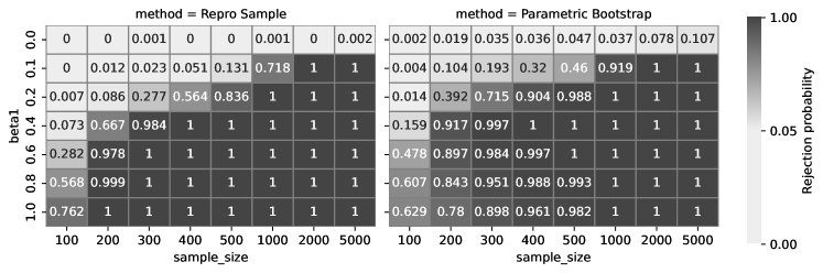
Figure 4: The rejection probability for hypothesis testing on $H_{0}:\beta_{1}^{*}=0$ and $H_{1}:\beta_{1}^{*}\neq 0$ in a linear regression model $Y=\beta_{0}^{*}+X\beta_{1}^{*}+\epsilon$ with repro and parametric bootstrap (Alabi and Vadhan, 2022). The significance level is 0.05, and the values in the table are calculated from 1000 replicates.

This example follows the setting in (Alabi and Vadhan, 2022), and we compare their parametric bootstrap method, Algorithm 2 in (Alabi and Vadhan, 2022), with our repro sample method. Consider the model $Y=\beta_{0}^{*}+X\beta_{1}^{*}+\epsilon$ where we want to test $H_{0}:\beta_{1}^{*}=0$ and $H_{1}:\beta_{1}^{*}\neq 0$. We assume $x_{i}\sim N(\mathbb{E}[X],\mathrm{Var}(X)),\varepsilon_{i}\sim N(0,\mathrm{Var}(\varepsilon)),y_{i}=\beta_{0}^{*}+x_{i}\beta_{1}^{*}+\epsilon_{i}$, and we let $\theta^{*}=(\beta_{1}^{*},\beta_{0}^{*},\mathbb{E}[X],\mathrm{Var}(X),\mathrm{Var}(\varepsilon))$ which fully parameterizes the model. Both the parametric bootstrap and our repro sample method use the sufficient statistic perturbation with Gaussian mechanism: Let $\tilde{\bar{x}}=\frac{1}{n}\sum_{i=1}^{n}[x_{i}]_{-\Delta}^{\Delta}+\frac{2\Delta}{(\mu/\sqrt{5})n}N_{1}$, $\widetilde{\mkern 1.5mu\overline{\mkern-1.5mux^{2}\mkern-1.5mu}\mkern 1.5mu}=\frac{1}{n}\sum_{i=1}^{n}{[x^{2}_{i}]_{0}^{\Delta^{2}}}+\frac{\Delta^{2}}{(\mu/\sqrt{5})n}N_{2}$, $\tilde{\bar{y}}=\frac{1}{n}\sum_{i=1}^{n}{[y_{i}]_{-\Delta}^{\Delta}}+\frac{2\Delta}{(\mu/\sqrt{5})n}N_{3}$, $\widetilde{\mkern 1.5mu\overline{\mkern-1.5muxy\mkern-1.5mu}\mkern 1.5mu}=\frac{1}{n}\sum_{i=1}^{n}{[x_{i}y_{i}]_{-\Delta^{2}}^{\Delta^{2}}}+\frac{2\Delta^{2}}{(\mu/\sqrt{5})n}N_{4}$, $\widetilde{\mkern 1.5mu\overline{\mkern-1.5muy^{2}\mkern-1.5mu}\mkern 1.5mu}=\frac{1}{n}\sum_{i=1}^{n}{[y_{i}^{2}]_{0}^{\Delta^{2}}}+\frac{\Delta^{2}}{(\mu/\sqrt{5})n}N_{5}$ where $N_{i}\overset{\text{iid}}{\sim}N(0,1)$; Releasing $s=(\tilde{\bar{x}},\widetilde{\mkern 1.5mu\overline{\mkern-1.5mux^{2}\mkern-1.5mu}\mkern 1.5mu},\tilde{\bar{y}},\widetilde{\mkern 1.5mu\overline{\mkern-1.5muxy\mkern-1.5mu}\mkern 1.5mu},\widetilde{\mkern 1.5mu\overline{\mkern-1.5muy^{2}\mkern-1.5mu}\mkern 1.5mu})$ is guaranteed to satisfy $\mu$-GDP. Using the released $s$, Alabi and Vadhan (2022) estimate $\theta$ and calculate the observed test statistic, then perform parametric bootstrap under the null hypothesis to compare the observed test statistic with the generated test statistics. In contrast, our Algorithm 3 finds the $\theta$ such that $s$ fits best into $(s_{i}(\theta))_{i=1}^{R}$ with respect to its Mahalanobis depth, and we compare the corresponding $p$-value with the significance level..

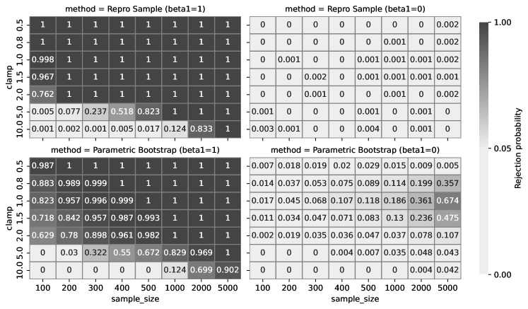
Figure 5: The rejection probability for hypothesis testing on $H_{0}:\beta_{1}^{*}=0$ and $H_{1}:\beta_{1}^{*}\neq 0$ in a linear regression model $Y=\beta_{0}^{*}+X\beta_{1}^{*}+\epsilon$ with repro and parametric bootstrap. The settings are the same as in Figure 4 except for the clamping region.

Our simulation results in Figure 4 show the rejection probability for $\beta_{1}^{*}=0$, 0.1, 0.2, 0.4, 0.6, 0.8, 1 under the settings of the sample size $n=100$, 200, 300, 400, 500, 1000, 2000, 5000, $R=200$, $\beta_{0}^{*}=-0.5$, $x_{i}\sim N(0.5,1)$, $\varepsilon_{i}\sim N(0,0.25)$, the clamping range $\Delta=2$, the significance level $\alpha=0.05$, and the privacy guarantee $1$-GDP. The rejection probability by our repro sample method is similar to the parametric bootstrap method except that when $\beta_{1}^{*}=0$ and $n\geq 2000$, the parametric bootstrap fails to control the type I error below the significance level of $0.05$, whereas our repro sample maintains conservative type I errors.

The success of our repro sample method is natural because of our finite sample guarantee in Theorem 4.1. Although Alabi and Vadhan (2022) proved in their Theorem 5.1 that their DP F-statistic converged in distribution to the asymptotic distribution of the non-private F-statistic, one of their assumptions is that $P(\exists i\in[n],y_{i}\notin[-\Delta_{n},\Delta_{n}])\rightarrow 0\text{ and }\forall i\in[n],\ x_{i}\in[-\Delta_{n},\Delta_{n}]$ as $n\rightarrow\infty$, which may be not achievable since $\Delta_{n}$ requires knowing the true parameters and every $x_{i}$. Without such knowledge, it is likely that $\Delta_{n}$ is chosen incorrectly and the clamping procedure effectively changes the data distribution. Furthermore, even if $\Delta_{n}$ is chosen correctly, the results of Alabi and Vadhan (2022) are only asymptotic, lacking finite-sample guarantees. We empirically verify this limitation by our simulation results in Figure 5, which shows the rejection probability for $\Delta=0.5$, 0.8, 1, 1.5, 2, 5, 10. In the bottom right subfigure of Figure 5, the parametric bootstrap drastically fails to maintain the significance level $0.05$ when $n\geq 2000$ and $\Delta=0.8$, 1, 1.5, 2; what is especially concerning is that the type I errors seem to get worse, rather than better, as the sample size increases. On the other hand, the type I errors for the repro approach is very well controlled, never exceeding 0.004. In addition to having better-controlled type I errors, our method also often has higher power, especially in smaller sample sizes. Additional simulations, where the privacy parameter $\mu$ is varied are found in Section B.2 of the supplement.

5.4 Logistic regression via objective perturbation

In this section, we demonstrate that our methodology can be applied to non-additive privacy mechanisms as well. In particular, we derive repro confidence intervals for a logistic regression model, using the objective perturbation mechanism (Chaudhuri and Monteleoni, 2008) with the formulation given in (Awan and Slavković, 2021), which adds noise to the gradient of the log-likelihood before optimizing, resulting in a non-additive privacy noise. However, since we assume that the predictor variables also need to be protected, we privatize their first two moments via the optimal $K$-norm mechanism (Hardt and Talwar, 2010; Awan and Slavković, 2021), a multivariate additive noise mechanism. Details for both mechanisms are in Section B.3 of the supplement.

We assume that the predictor variable $x$ is naturally bounded in some known interval, and normalized to take values in $[-1,1]$. We model $x$ in terms of the beta distribution: $x_{i}=2z_{i}-1$, where $z_{i}\overset{\text{iid}}{\sim}\mathrm{Beta}(a^{*},b^{*})$. Then $y|x$ comes from a logistic regression: $y_{i}|x_{i}\sim\mathrm{Bern}(\mathrm{expit}(\beta_{0}^{*}+\beta_{1}^{*}x_{i}))$, where $\mathrm{expit}(x)=\exp(x)/(1+\exp(x))$. In this problem, the parameter is $\theta^{*}=(\beta_{0}^{*},\beta_{1}^{*},a^{*},b^{*})$, and we are primarily interested in $\beta_{1}^{*}$.

To set up the generating equation, we use inverse transform sampling for $z_{i}$: $z_{i}=F^{-1}_{a^{*},b^{*}}(u_{i})$, where $F_{a^{*},b^{*}}^{-1}$ is the quantile function of $\mathrm{Beta}(a^{*},b^{*})$, and $u_{i}\overset{\text{iid}}{\sim}U(0,1)$; similarly, we generate $y_{i}=I(w_{i}\leq\mathrm{expit}(\beta_{0}^{*}+\beta_{1}^{*}x_{i}))$, where $w_{i}\overset{\text{iid}}{\sim}U(0,1)$. The privatized output $s$ consists of estimates of $(\beta_{0}^{*},\beta_{1}^{*})$ from objective perturbation, as well as noisy estimates of the first two moments of the $z_{i}$’s, privatized by a $K$-norm mechanism. Since the only source of randomness in the two privacy mechanisms are independent variables from $K$-norm distributions, we use the $K$-norm random variables as the “seeds” for the privacy mechanisms. See Section B.2 of the supplement for details about objective perturbation and $K$-norm mechanisms.

In the simulation generating the results in Figure 6, we let $a^{*}=b^{*}=0.5$, $\beta_{0}^{*}=0.5$, $\beta_{1}^{*}=2$, $R=200$, $\alpha=0.05$, $n=100,$ 200, 500, 1000, 2000, and $\varepsilon=0.1$, 0.3, 1, 3, 10 in $\varepsilon$-DP. Other details for this experiment are found in Section B.3 of the supplement.

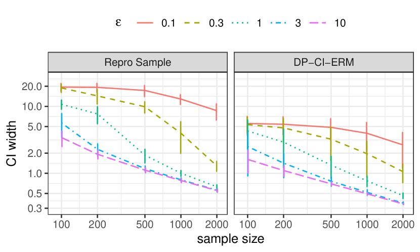
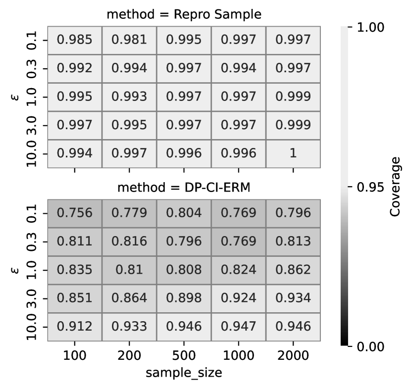
Figure 6: Width and coverage for the confidence intervals of $\beta_{1}$ in logistic regression with repro and DP-CI-ERM (Wang et al., 2019). Parameters for this simulation are $a^{*}=b^{*}=0.5$, $\beta_{0}^{*}=0.5$, $\beta_{1}^{*}=2$, $R=200$, $\alpha=0.05$, and the results were averaged over 1000 replicates.

In Figure 6, we compare the width and coverage of the repro confidence intervals using Mahalanobis depth, against an alternative method proposed by Wang et al. (2019), which develops a joint privacy mechanism and confidence interval algorithm for empirical risk minimization problems which is also based on objective perturbation (we refer to this method as DP-CI-ERM). Some key differences between the repro approach and DP-CI-ERM are 1) repro allows for arbitrary privacy mechanisms, whereas DP-CI-ERM requires one to use a specific privacy mechanism, 2) repro requires a fully parametric model, whereas DP-CI-ERM only needs the empirical risk function, 3) repro gives finite sample coverage guarantees, whereas DP-CI-ERM gives an asymptotic coverage guarantee, and 4) repro confidence interval is for the true parameter while DP-CI-ERM uses regularized loss function and its confidence interval is for the regularized population risk minimizer, which is not the parameter of interest. Because of these differences, this comparison is somewhat apples-to-oranges, but is still instructive to understand the pros and cons of the repro methodology. We see in Figure 6 that DP-CI-ERM generally has smaller confidence interval width compared to repro, considering a variety of sample sizes and privacy budgets – roughly, the widths for repro are about 2-4 times as wide as those for DP-CI-ERM. However, while the coverage of DP-CI-ERM is very close to 0.95 at large sample sizes or large $\varepsilon$ values, we see that it has significant under coverage in several settings of $n$ and $\epsilon$. On the other hand, we see that repro always has greater than 95% coverage.

6 Discussion

We have shown that simulation-based inference is a powerful technique that enables finite-sample frequentist confidence intervals and hypothesis tests on privatized data. We have shown through several examples that the repro methodology offers more reliable, and sometimes even more powerful inference compared to existing methods, such as the parametric bootstrap. We have also improved the original repro methodology to account for Monte Carlo errors, and emphasize that while our results were motivated by problems in differential privacy, our inference framework is also applicable to models outside of privacy.

A limitation of the repro methodology is that it is generally not guaranteed that the resulting confidence set will be connected, and due to this limitation, it can be difficult to ensure that all regions of the confidence set have been found. Algorithm 2 relies on the assumption that the confidence set of interest is in fact an interval, and may not achieve the target coverage if this assumption is false. Nevertheless, our simulations have demonstrated that in all of the settings considered, our repro confidence intervals via Algorithm 2 have coverage above the nominal level. Future researchers may investigate necessary and sufficient conditions for the repro confidence sets to be connected as well as alternative algorithms to obtain the repro confidence sets.

6.1 Choice of test statistic

The ideal test statistic for use in repro would be a pivot, whose formula and sampling distribution do not depend on the nuisance parameters, as this avoids the issue of over-coverage as well as reduces the computation burden of optimizing over the nuisance parameters. However, finding a pivot is not always possible. Especially in the setting of differential privacy, it is very challenging to design test statistics whose distribution does not depend on nuisance parameters (e.g., Gaboardi et al. (2016); Du et al. (2020); Awan and Vadhan (2021); Alabi and Vadhan (2022)). As Xie and Wang (2022) suggested, the goal is then to find an approximate pivot, such as one whose asymptotic distribution does not depend on the nuisance parameters. While classical statistical methods suggest plugging in an estimator for the nuisance parameters to approximate the sampling distribution using asymptotic theory, there is no finite sample guarantee that this will give accurate coverage/type I error rates. On the other hand, using repro samples, we can still get the benefit of using an approximate pivot, while still ensuring coverage/type I error rates. See Section B.4 of the supplement for an example where we construct a custom test statistic and demonstrate the improved coverage compared to the depth statistic. A problem for future work would be to develop general strategies to construct approximate pivots from DP statistics, which can both reduce the over-coverage and optimize the test statistic for the model and mechanism at hand.

On the other hand, most of the examples considered in this paper used a depth statistic as the default test statistic in repro. In this section, we quantify the suboptimality of this approach in terms of increased width/decreased power. There are two main issues at play: 1) The depth statistic may generally be a sub-optimal test statistic and 2) Because we are implicitly obtaining a simultaneous confidence set for all $d$ parameters, assuming that the marginal coverages of each projected confidence set are roughly equal, we would expect each coverage to be $(1-\alpha)^{1/d}$, resulting in an increased width.

While there is often a loss in power from using a default test statistic, such as a depth statistic, it is difficult to quantify the suboptimality, as this is problem specific.

$d$	1	2	5	10	100	1000
Relative width	1	1.14	1.31	1.43	1.77	2.07

Table 2: Relative width due to over-coverage for the normal mean with known variance, when the nominal level is $1-\alpha=0.95$, and the over-coverage level is $1-\alpha^{*}=(1-\alpha)^{1/d}$.

To understand the cost of over-coverage, we consider as an idealized setting the widths of confidence intervals on normal data – this is a useful example since many statistics are asymptotically normal. We explore the increased width due to over-coverage when $\alpha=0.05$ and $d$ increases in Table 2. We see having a single nuisance parameter increases the width by 14%, but that as $d$ increases, the increase in the width is very slow, requiring $d=1000$ before we have about twice the width. So, while over-coverage does increase the width of our intervals, the increased width is often within a factor of 1.5-2, even for a large number of nuisance parameters. For a fixed nominal level $\alpha$, the relative width of the normal confidence interval grows proportionally to $\sqrt{\log(d)}$, a very slow rate (see Proposition A.3 in the supplement).

Appendix A Proofs and technical details

Lemmas similar to the following have been used in conformal prediction to guarantee coverage rates for the predictions. We include proofs of the lemmas for completeness.

Lemma A.1.

Let $x_{1},\ldots,x_{n}$ be an exchangeable sequence of real-valued random variables. Then $P(x_{(a)}\leq x_{n})\geq\frac{n-a+1}{n}$, $P(x_{n}\leq x_{(b)})\geq\frac{b}{n}$, and $P(x_{(a)}\leq x_{n}\leq x_{(b)})\geq\frac{(b-a+1)}{n}$, where $x_{(a)}$ and $x_{(b)}$ are the $a^{th}$ and $b^{th}$ order statistics of $x_{1},\ldots,x_{n}$. Furthermore, for $a_{\alpha}=\lfloor\alpha n\rfloor+1$, $P(x_{(a_{\alpha})}\leq x_{n})\geq 1-\alpha$, and for $b_{\alpha}=\lceil(1-\alpha)n\rceil$, $P(x_{n}\leq x_{(b_{\alpha})})\geq 1-\alpha$. For any $a=1,2,\ldots,n-\lceil(1-\alpha)n\rceil+1$, setting $b=a+\lceil(1-\alpha)n\rceil-1$ ensures that $P(x_{(a)}\leq x_{n}\leq x_{(b)})\geq 1-\alpha$.

Proof.

Notice that $x_{n}$ is equally likely to take any of the $n$ positions. In the first case, there are $a-1$ positions not in the interval (assuming no ties), so there are $n-a+1$ positions that make the probability true. In the second case, there are $b$ positions that make the probability true, and in the third case, there are $(b-a+1)$ positions in the interval. If there are ties at the boundaries, then each of these counts only increases.

For $a_{\alpha}$ and $b_{\alpha}$ defined above, note that $P(x_{(a_{\alpha})}\leq x_{n})\geq\frac{n-(a_{\alpha}-1)}{n}=\frac{n-\lfloor\alpha n\rfloor}{n}\geq 1-\alpha,$ and $P(x_{n}\leq x_{(b_{\alpha})})\geq\frac{b_{\alpha}}{n}=\frac{\lceil(1-\alpha)n\rceil}{n}\geq 1-\alpha.$ Finally, let $a$ and $b$ be any values such that $b-a=\lceil(1-\alpha)n\rceil-1$. Then by the earlier result, we have $P(x_{(a)}\leq x_{n}\leq x_{(b)})\geq(b-a+1)/n=\lceil(1-\alpha)n\rceil/n\geq(1-\alpha).$∎

Lemma A.2.

Let $x_{1},\ldots,x_{n}$ be an exchangeable sequence of real-valued random variables. Then $p=n^{-1}\#\{x_{i}\leq x_{1}\}$ satisfies $P(p\leq\alpha)\leq\alpha$.

Proof.

First, let $k\in\{0,1,2,\ldots,n-1\}$, and consider $P(\#\{x_{i}\geq x_{1}\}\leq k)=P(x_{1}>x_{(n-k)})=1-P(x_{1}\leq x_{(n-k)})\leq 1-(n-k)/n=k/n,$ where we used Lemma A.1 to establish the inequality. Now, setting $k=\lfloor n\alpha\rfloor$, we have that

$$P(p\leq\alpha)=P(\#\{x_{i}\geq x_{1}\}\leq n\alpha)=P(\#\{x_{i}\geq x_{1}\}\leq\lfloor n\alpha\rfloor)=\lfloor n\alpha\rfloor/n\leq\alpha.\qed$$

Proof of Lemma 3.1..

The fact that $\Gamma_{\alpha}(s,u)$ is a $(1-\alpha)$-confidence set is easily seen from the following: $P_{s\sim F_{\theta},u}(\theta\in\Gamma_{\alpha}(s,u))=P_{s\sim F_{\theta},u}(B_{\alpha}(\theta;s,u))\geq 1-\alpha.$ Note that $\Gamma^{\beta}_{\alpha}(s,u)\times\{\eta|\exists\beta^{*}\text{ s.t. }(\beta^{*},\eta)\in\Theta\}\supset\Gamma_{\alpha}(s,u)$. It follows that

$$P_{s\sim F_{(\beta,\eta)},u}(\beta\in\Gamma_{\alpha}^{\beta}(s,u))\geq P_{s\sim F_{(\beta,\eta)},u}((\beta,\eta)\in\Gamma_{\alpha}(s,u))\geq 1-\alpha.$$

To see that $\Gamma_{\alpha}^{\theta_{1}}(s,u),\ldots,\Gamma_{\alpha}^{\theta_{k}}(s,u)$ are simultaneous $(1-\alpha)$-confidence sets for $\theta_{1},\ldots,\theta_{k}$, consider

$$P_{s\sim F_{(\theta_{1},\ldots,\theta_{k})},u}(\theta_{1}\in\Gamma_{\alpha}^{\theta_{1}}(s,u),\ldots,\theta_{k}\in\Gamma_{\alpha}^{\theta_{k}}(s,u)) =P_{s\sim F_{\theta},u}(\theta\in\Gamma_{\alpha}^{\theta_{1}}(s,u)\times\cdots\times\Gamma_{\alpha}^{\theta_{k}}(s,u))$$

$$\geq P_{s\sim F_{\theta},u}(\theta\in\Gamma_{\alpha}(s,u))$$

$$\geq 1-\alpha,$$

since $\Gamma_{\alpha}^{\theta_{1}}(s,u)\times\cdots\times\Gamma_{\alpha}^{\theta_{k}}(s,u)\supset\Gamma_{\alpha}(s,u)$. ∎

Proof of Theorem 3.6..

The fact that $B_{\alpha}(\theta;s,(u_{i})_{i=1}^{R})$ satisfies (1) follows from Lemma A.1, since $T_{\theta}(s;s,s_{1}(\theta),\ldots,s_{R}(\theta)),$ $T_{\theta}(s_{1}(\theta);s,s_{1}(\theta),\ldots,s_{R}(\theta)),\ldots,T_{\theta}(s_{R}(\theta);s,s_{1}(\theta),\ldots,s_{R}(\theta))$ are exchangeable. It follows from Lemma 3.1 that both $\Gamma_{\alpha}(s,u)$ and $\Gamma_{\alpha}^{\beta}(s,u)$ are $(1-\alpha)$-confidence sets. ∎

Proof of Proposition 3.12..

We can express the target confidence interval in the following way:

$$\Gamma_{\alpha}^{\beta}(s,u) =\{\beta|\exists\eta\text{ s.t. }I(B_{\alpha}((\beta,\eta);s,u))=1\}$$

$$=\{\beta|\exists\eta\text{ s.t. }T_{\text{obs}}(\beta,\eta)\geq T_{(a)}(\beta,\eta)\}$$

$$=\left\{\beta\middle|\exists\eta\text{ s.t. }\#\{T_{\text{obs}}(\beta,\eta)\geq T_{(i)}(\beta,\eta)\}\geq a\right\}$$

$$=\left\{\beta\middle|\sup_{\eta}\#\{T_{\text{obs}}(\beta,\eta)\geq T_{(i)}(\beta,\eta)\}\geq a\right\}$$

$$=\left\{\beta\middle|\sup_{\eta}\Big{(}\#\{T_{\text{obs}}(\beta,\eta)\geq T_{(i)}(\beta,\eta)\}+T_{\text{obs}}(\beta,\eta)\Big{)}\geq a\right\},$$

where the last line uses the assumption that $T(\beta,\eta)$ takes values in $[0,1]$, the observation that $T_{\text{obs}}(\beta,\eta)=1$ only if $\#\{T_{\text{obs}}(\beta,\eta)\geq T_{(i)}(\beta,\eta)\}=R+1$, and the fact that $a\in\mathbb{Z}$.

We see that $\texttt{accept}(\beta,\alpha,\Theta=B\times H,(u_{i})_{i=1}^{R},G,s,T)$ returns TRUE if and only if $\beta\in\Gamma_{\alpha}^{\beta}(s,u)$. Then, given $\hat{\beta}_{\mathrm{init}}\in\Gamma_{\alpha}^{\beta}(s,u)$ and the values $\beta_{L},\beta_{U}\not\in\Gamma_{\alpha}^{\beta}(s,u)$, we see that the bisection method returns the boundary points of $\Gamma_{\alpha}^{\beta}(s,u)$. ∎

Proof of Theorem 4.1..

For any $\theta_{0}\in\Theta_{0}$, call $p(s;\theta_{0})=\frac{1}{R+1}[\#\{T_{(i)}(\theta_{0})\leq T_{\text{obs}}(\theta_{0})\}]$, which due to the exchangeability of the $T_{(i)}(\theta_{0})$ is a valid $p$-value for $H_{0}:\theta^{*}=\theta_{0}$, according to Lemma A.2. Then we can write $p=\frac{\sup_{\theta\in\Theta_{0}}\#\{T_{(i)}(\theta)\leq T_{\text{obs}}(\theta)\}}{R+1}$ as $p=\sup_{\theta\in\Theta_{0}}p(s;\theta).$ Then, since $p\geq p(s;\theta^{*})$, where $\theta^{*}\in\Theta_{0}$ is the true parameter value, we have $P_{s\sim F_{\theta^{*}}}(p\leq\alpha)\leq P_{s\sim F_{\theta^{*}}}(p(s;\theta^{*})\leq\alpha)\leq\alpha,$ and we see that $p$ is a valid $p$-value for $H_{0}$. ∎

Proof of Proposition 4.2..

Note that since $T$ takes values in $[0,1]$, $\lfloor M\rfloor=\sup_{\theta\in\Theta_{0}}\#\{T_{i}(\theta)\leq T_{\text{obs}}(\theta)\}$ unless $T_{\text{obs}}(\theta)=1$. When $T_{\text{obs}}(\theta)=1$ we have $T_{\text{obs}}(\theta)\geq T_{i}(\theta)$ for all $i=1,2,\ldots,R$, giving $\lfloor M\rfloor=R+1$, whereas $\#\{T_{i}(\theta)\leq T_{\text{obs}}(\theta)\}=R$. We conclude that $\min\{\lfloor M\rfloor+1,R+1\}=\sup_{\theta\in\Theta_{0}}\#\{T_{i}(\theta)\leq T_{\text{obs}}(\theta)\}+1=\sup_{\theta\in\Theta_{0}}\#\{T_{(i)}(\theta)\leq T_{\text{obs}}(\theta)\}$. We see that $p$, the output of $\texttt{pvalue}(\Theta_{0},(u_{i})_{i=1}^{R},G,s,T)$ is equal to $\frac{\sup_{\theta\in\Theta_{0}}\#\{T_{(i)}(\theta)\leq T_{\text{obs}}(\theta)\}}{R+1}$, as desired. ∎

Proposition A.3.

Let $\alpha\in(0,1)$. Then $\sqrt{\log(1/(1-(1-\alpha)^{1/d}))}\sim\sqrt{\log(d)}$, as $d\rightarrow\infty$.

Proof.

Our goal is to show that $\lim_{d\rightarrow\infty}\frac{\sqrt{(-1)\log(1-(1-\alpha)^{1/d})}}{\sqrt{\log(d)}}=1.$ First, we will evaluate the limit without the square root:

$$\lim_{d\rightarrow\infty}\frac{(-1)\log(1-(1-\alpha)^{1/d})}{\log(d)} \overset{\text{L'H}}{=}\lim_{d\rightarrow\infty}\frac{d(-1)\log(1-\alpha)(1-\alpha)^{1/d}}{d^{2}(1-(1-\alpha)^{1/d})}$$

$$\overset{\phantom{\text{L'H}}}{=}\lim_{d\rightarrow\infty}\frac{(-1)\log(1-\alpha)(1-\alpha)^{1/d}(1/d)}{1-(1-\alpha)^{1/d}}$$

$$\overset{\text{L'H}}{=}\lim_{d\rightarrow\infty}\frac{\log(1-\alpha)(1-\alpha)^{1/d}(\log(1-\alpha)+d)d^{2}}{d^{3}\log(1-\alpha)(1-\alpha)^{1/d}}$$

$$\overset{\phantom{\text{L'H}}}{=}\lim_{d\rightarrow\infty}\frac{\log(1-\alpha)+d}{d}$$

$$=1,$$

where “$\overset{\text{L'H}}{=}$” indicates that we used L’Hôpital’s rule. Finally, since $\sqrt{\cdot}$ is a continuous function at $1$, applying $\sqrt{\cdot}$ to both sides gives the desired result. ∎

Appendix B Additional simulation details and results

B.1 Exponential distribution

Suppose that $x_{1},\ldots,x_{n}\overset{\text{iid}}{\sim}\mathrm{Exp}(\mu^{*})$, where $\mu^{*}$ is the scale/mean parameter. We assume that we have some pre-determined threshold $c$, and the data will be clamped to lie in the interval $[0,c]$. Our privatized statistic is $s=\frac{1}{n}\sum_{i=1}^{n}[x_{i}]_{0}^{c}+\frac{c}{n\varepsilon}N$, where $N$ is a noise adding mechanism; for this example, we will assume that $N\sim\mathrm{Laplace}(0,1)$, which ensures that $s$ satisfies $\varepsilon$-DP. Note that there are two complications to understanding the sampling distribution of $s$: the clamping and the noise addition.

We will show that for the exponential distribution, we can derive the characteristic function for $[x_{i}]_{0}^{c}$, which we will call $\phi_{\mu^{*}}$. Then the characteristic function for $s$ is

$$\phi_{s,\mu^{*}}(t)=(\phi_{\mu^{*}}(t/n))^{n}\phi_{N}((c/(n\varepsilon))t),$$

where $\phi_{N}$ is the characteristic function for $N$. Once we have $\phi_{s}$, we can use inversion formulae to evaluate the cdf and pdf. This strategy was first proposed for DP statistical analysis in Awan and Vadhan (2021) in the context of privatized difference of proportions tests.

$$\phi_{\mu^{*}}(t) =\mathbb{E}_{x\sim\mu^{*}}e^{it[x]_{0}^{c}}$$

$$=\int_{0}^{c}e^{itx}\frac{1}{\mu^{*}}e^{-x/\mu^{*}}\ dx+e^{itc}P_{x\sim\mu^{*}}(x\geq c)$$

$$=\int_{0}^{c}\frac{1}{\mu^{*}}e^{x(-1/\mu^{*}+it)}\ dx+e^{itc}e^{-c/\mu^{*}}$$

$$=\frac{e^{x(-1/\mu^{*}+it)}}{\mu^{*}(-1/\mu^{*}+it)}\Big{|}_{0}^{c}+e^{itc-c/\mu^{*}}$$

$$=\frac{1-e^{c(it-1/\mu^{*})}}{1-it\mu^{*}}+e^{itc-c/\mu^{*}}.$$

Note that while $[x]_{0}^{c}$ is not a continuous distribution, the Laplace noise makes $s$ continuous. So, Gil-Pelaez inversion tells us that we can evaluate the cdf $F_{s,\mu^{*}}$ as

$$F_{s,\mu^{*}}(x)=\frac{1}{2}-\frac{1}{\pi}\int_{0}^{\infty}\frac{\mathrm{Im}(e^{-itx}\phi_{s,\mu^{*}}(t))}{t}\ dt,$$

which can be solved by numerical integration, such as by integrate command in R. We can then use the cdf to determine a level $\alpha$ set by finding the $(1-\alpha)/2$ and $1-(1-\alpha)/2$ quantiles, for example by the bisection method (relies on the fact that $F_{s,\mu^{*}}(x)$ is monotone in $\mu^{*}$ for a fixed $s$ and $x$). Based on the general description above, we then determine which $\mu^{*}$ values lie in these intervals. However, we can actually skip the creation of the level $\alpha$ sets by simply checking for each $\mu^{*}$ whether $F_{s,\mu^{*}}(s)\in[(1-\alpha)/2,1-(1-\alpha)/2]$. In this case, we only need to perform two bisection method searches to determine the lower and upper confidence limits for $\mu^{*}$.

Note that by using characteristic functions, the computational complexity does not depend on $n$ at all, making this approach tractable for both small and large sample sizes. While there can potentially be some numerical instability in the integration step, we found that it was not a significant problem.

In Table 3, we see the result of a simulation study, using the confidence interval procedure described above for the exponential distribution. We used the parameters $n=100$, $\varepsilon=1$, $\mu^{*}=10$, $\alpha=0.95$, and varied $c$. We include the empirical coverage and average confidence interval width over 1000 replicates. The coverage is very close to the provable $0.95$ coverage level. While one may expect the width to depend on the $c$ parameter, and we did indeed find larger widths with very small and very large $c$, even with extreme values of $c$, we still had an informative confidence interval, with the width of the smallest interval (from $c=20$) being 4.906, and the width of the largest interval (from $c=100$) being 7.153.

		$c=10$	$c=20$	$c=50$	$c=100$
	Coverage	0.936(0.008)	0.935(0.008)	0.938(0.008)	0.955(0.007)
Inversion	Average Width	6.066(0.041)	4.919(0.023)	5.030(0.014)	7.144(0.011)
	Coverage	0.005(0.002)	0.785(0.013)	0.947(0.007)	0.957(0.006)
PB	Average Width	1.474(0.001)	2.696(0.004)	4.692(0.011)	7.007(0.014)

Table 3: 95% confidence intervals for clamped exponential distribution with Laplace noise. $n=100$, $\varepsilon=1$, $\mu^{*}=10$, number of replicates $1000$. Top row is based on the inversion of characteristic functions, bottom is from the parametric bootstrap (simplified-$t$ intervals).

B.2 More simulations with simple linear regression hypothesis testing

We show more simulation results in Figure 8 and 8, where we vary the privacy parameter $\mu$. We can see that when $\mu\geq 0.5$ for $\mu$-GDP and sample size $n=5000$, the type I error of the parametric bootstrap method (Alabi and Vadhan, 2022) is higher than the significance level $\alpha=0.05$, while the repro sample method always controls the type I error well. Although the power of the two methods is comparable, the repro sample method follows our intuition that when $\beta_{1}$ is further away from 0, the power is larger, for all settings of sample size and privacy requirement, while the parametric bootstrap method does not.

Figure 7: The rejection probability for hypothesis testing on $H_{0}:\beta_{1}^{*}=0$ and $H_{1}:\beta_{1}^{*}\neq 0$ in a linear regression model $Y=\beta_{0}^{*}+X\beta_{1}^{*}+\epsilon$ with repro sample method. We compare the results with different privacy settings of $\mu$-GDP: $\mu=10$, 5, 2, 0.5, 0.2, 0.1, 0.05, 0.01. (Figure 4 of Section 5.3 shows the result of $\mu=1$.) The significance level is 0.05, and the values in the table are calculated from 1000 replicates.

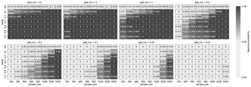
Figure 8: The rejection probability for hypothesis testing on $H_{0}:\beta_{1}^{*}=0$ and $H_{1}:\beta_{1}^{*}\neq 0$ in a linear regression model $Y=\beta_{0}^{*}+X\beta_{1}^{*}+\epsilon$ with parametric bootstrap (Alabi and Vadhan, 2022). We compare the results with different privacy settings of $\mu$-GDP: $\mu=10$, 5, 2, 0.5, 0.2, 0.1, 0.05, 0.01. (Figure 4 of Section 5.3 shows the result of $\mu=1$.) The significance level is 0.05, and the values in the table are calculated from 1000 replicates.

B.3 Details for logistic regression simulation

We assume that the space of datasets is of the form $\mathscr{D}=\mathscr{X}^{n}$, and that the adjacency metric $d$ is the Hamming distance. For the logistic regression application in Section 5.4, we use techniques from Awan and Slavković (2021), including the sensitivity space, $K$-norm mechanisms, and objective perturbation. In order to be self-contained, we include the basic definitions and algorithms in this section.

Definition B.1 (Sensitivity Space: Awan and Slavković, 2021).

Let $T:\mathscr{X}^{n}\rightarrow\mathbb{R}^{m}$ be any function. The sensitivity space of $T$ is

$$S_{T}=\left\{u\in\mathbb{R}^{m}\middle|\begin{array}[]{c}\exists X,X^{\prime}\in\mathscr{X}^{n}\text{ s.t }d(X,X^{\prime})=1\\ \text{and }u=T(X)-T(X^{\prime})\end{array}\right\}.$$

A set $K\subset\mathbb{R}^{m}$ is a norm ball if $K$ is 1) convex, 2) bounded, 3) absorbing: $\forall u\in\mathbb{R}^{m}$, $\exists c>0$ such that $u\in cK$, and 4) symmetric about zero: if $u\in K$, then $-u\in K$. If $K\subset\mathbb{R}^{m}$ is a norm ball, then $\lVert u\rVert_{K}=\inf\{c\in\mathbb{R}^{\geq 0}\mid u\in cK\}$ is a norm on $\mathbb{R}^{m}$.

Algorithm 4 Sampling $\propto\exp(-c\lVert V\rVert_{\infty})$ (Steinke and Ullman, 2016)

INPUT: $c$, and dimension $m$

1: Set $U_{j}\overset{\text{iid}}{\sim}U(-1,1)$ for $j=1,\ldots,m$

2: Draw $r\sim\mathrm{Gamma}(\alpha=m+1,\beta=c)$

3: Set $V=r\cdot(U_{1},\ldots,U_{m})^{\top}$

OUTPUT: $V$

The sensitivity of a statistic $T$ is the largest amount that $T$ changes when one entry of $T$ is modified. Geometrically, the sensitivity of $T$ is the largest radius of $S_{T}$ measured by the norm of interest. For a norm ball $K\subset\mathbb{R}^{m}$, the $K$-norm sensitivity of $T$ is

$$\Delta_{K}(T)=\sup_{d(X,X^{\prime})=1}\lVert T(X)-T(X^{\prime})\rVert_{K}=\sup_{u\in S_{T}}\lVert u\rVert_{K}.$$

Algorithm 5 Sampling $K$-Norm Mechanism with Rejection Sampling (Awan and Slavković, 2021)

INPUT: $\varepsilon$, statistic $T(X)$, $\ell_{\infty}$ sensitivity $\Delta_{\infty}(T)$, $K$-norm sensitivity $\Delta_{K}(T)$

1: Set $m=\mathrm{length}(T(X))$.

2: Draw $r\sim\mathrm{Gamma}(\alpha=m+1,\beta=\varepsilon/\Delta_{K}(T))$

3: Draw $U_{j}\overset{\text{iid}}{\sim}\mathrm{Uniform}(-\Delta_{\infty}(T),\Delta_{\infty}(T))$ for $j=1,\ldots,m$

4: Set $U=(U_{1},\ldots,U_{m})^{\top}$

5: If $U\in K$, set $N_{K}=U$, else go to 3)

6: Release $T(X)+N_{K}$.

Algorithm 6 $\ell_{\infty}$ Objective Perturbation (Awan and Slavković, 2021)

INPUT: $X\in\mathscr{X}^{n}$, $\varepsilon>0$, a convex set $\Theta\subset\mathbb{R}^{m}$, a convex function $r:\Theta\rightarrow\mathbb{R}$, a convex loss $\hat{\mathscr{L}}(\theta;X)=\frac{1}{n}\sum_{i=1}^{n}\ell(\theta;x_{i})$ defined on $\Theta$ such that $\nabla^{2}\ell(\theta;x)$ is continuous in $\theta$ and $x$, $\Delta>0$ such that $\sup_{x,x^{\prime}\in\mathscr{X}}\sup_{\theta\in\Theta}\lVert\nabla\ell(\theta;x)-\nabla\ell(\theta;x^{\prime})\rVert_{\infty}\leq\Delta$, $\lambda>0$ is an upper bound on the eigenvalues of $\nabla^{2}\ell(\theta;x)$ for all $\theta\in\Theta$ and $x\in\mathscr{X}$, and $q\in(0,1)$.

1: Set $\gamma=\frac{\lambda}{\exp({\varepsilon(1-q)})-1}$

2: Draw $V\in\mathbb{R}^{m}$ from the density $f(V;\varepsilon,\Delta)\propto\exp(-\frac{\varepsilon q}{\Delta}\lVert V\rVert_{\infty})$ using Algorithm 4

3: Compute $\theta_{DP}=\arg\min_{\theta\in\Theta}\hat{\mathscr{L}}(\theta;X)+\frac{1}{n}r(\theta)+\frac{\gamma}{2n}\theta^{\top}\theta+\frac{V^{\top}\theta}{n}$

OUTPUT: $\theta_{DP}$

The privacy mechanism consists of two components, each of dimension 2: to encode information about the parameters $a$ and $b$, we release $(\sum_{i=1}^{n}z_{i},\sum_{i=1}^{n}z_{i}^{2})+N_{K}$, where $N_{K}$ is from a $K$-norm mechanism that discuss in the following paragraphs; to learn $\beta_{0}$ and $\beta_{1}$, we run Algorithm 6. In Awan and Slavković (2021, Section 4.1), it was calculated that $\Delta_{\infty}=2$ and $\lambda=m/4$; In Awan and Slavković (2021, Section 4.2), it was numerically found that $q=0.85$ optimized the performance of objective perturbation. Awan and Slavković (2021, Theorem 4.1) showed that the output of Algorithm 6 satisfies $\varepsilon$-DP.

Awan and Slavković (2021) showed that the optimal $K$-norm mechanism (in terms of quantities such as stochastic tightness, minimum entropy, and minimum conditional variance) of a statistic $T(X)$ uses the norm ball, which is the convex hull of the sensitivity space. For the statistic $T(X)=(\sum_{i=1}^{n}z_{i},\sum_{i=1}^{n}z_{i}^{2})$, where $z_{i}\in[0,1]$, we can derive the sensitivity space as

Figure 9: In dark blue is the sensitivity space derived in Equation (5). In light blue and dark blue is the convex hull of the sensitivity space, derived in Equation (6).

$$S_{T}=\left\{(u_{1},u_{2})\middle|\begin{array}[]{c}u_{1}^{2}\leq u_{2}\leq 1-(u_{1}-1)^{2}\\ \text{or }\quad(1+u_{1})^{2}-1\leq u_{2}\leq u_{1}^{2}\end{array}\right\},$$ (5)

and the convex hull can be expressed as

$$\mathrm{Hull}(S_{T})=\left\{(u_{1},u_{2})\middle|\begin{array}[]{cc}(u_{1}+1)^{2}-1\leq u_{2}\leq-u_{1}^{2},&u_{1}\leq-1/2\\ u_{1}-1/4\leq u_{2}\leq u_{1}+1/4,&-1/2<u_{1}\leq 1/2\\ u_{1}^{2}\leq u_{2}\leq 1-(u_{1}-1)^{2},&1/2\leq u_{1}\end{array}\right\}.$$ (6)

We use $K=\mathrm{Hull}(S_{T})$ as the norm ball in Algorithm 5, which Hardt and Talwar (2010) showed satisfies $\varepsilon$-DP.

In the simulation generating the results in Figure 6 of Section 5.4, we let $a^{*}=b^{*}=0.5$, $\beta_{0}^{*}=0.5$, $\beta_{1}^{*}=2$, $R=200$, $\alpha=0.05$, $n=100,$ 200, 500, 1000, 2000, and $\varepsilon=0.1$, 0.3, 1, 3, 10 in $\varepsilon$-DP. For the repro sample method, the private statistics we release and use are $s=(\tilde{\beta}_{0},\tilde{\beta}_{1},\tilde{T}(X))$ where $(\tilde{\beta}_{0}$, $\tilde{\beta}_{1})$ are the output of Algorithm 6 with $0.9\varepsilon$-DP, $q=0.85$, $\lambda=1/4$, and $\tilde{T}(X)$ is the output of Algorithm 5, with private budget $0.1\varepsilon$. When using Algorithm 4 and 5, we let $m=2$ as it is the dimension of the output.

For the DP-CI-ERM (Wang et al., 2019), we use their Algorithm 1 (Objective Perturbation) with $\varepsilon/2$-DP, $t=1/4$, $c=t/(2n)/(\mathrm{e}^{(1-q)\varepsilon/2}-1)$, $q=0.85$, and we use their Algorithm 2 to obtain the private estimations of the covariance matrix and the Hessian matrix, both with $\varepsilon/4$-DP and the same $c$ as in the Objective Perturbation; in their Algorithm 5, we set $m=10,000$. For the data used in our simulation, since Wang et al. (2019) had an assumption $\|\vec{x}_{i}\|_{2}\leq 1$ in their Theorem 1, we map our generated covariate $(1,x_{i})$ to $(\frac{1}{\sqrt{2}},\frac{x_{i}}{\sqrt{2}})$ to satisfy their assumption as our generated $x_{i}\in[-1,1]$. After this covariate transformation, the true coefficient is changed to $(\sqrt{2}\beta_{0},\sqrt{2}\beta_{1})$; therefore, we scale the estimated coefficient back for an appropriate comparison on the width of the confidence intervals. We also map our generated $y\in\{0,1\}$ to $y^{\prime}=2y-1$ since the loss function and corresponding analysis of the logistic regression in (Wang et al., 2019) was based on the response being $y^{\prime}\in\{-1,1\}$.

For both the repro sample method and DP-CI-ERM, we compute the confidence interval within the range $[-10,10]$.

B.4 Private Bernoullis with unknown $n$

Awan and Slavković (2018), Awan and Slavković (2020), and Awan and Vadhan (2021) derived optimal private hypothesis tests and confidence intervals for Bernoulli data, under $(\varepsilon,\delta)$-DP as well as general $f$-DP, but assumed that the sample size $n$ was known as they worked in the bounded-DP setting. In the framework of bounded-DP, it is assumed that $n$ is public knowledge, and two databases are neighboring if they differ in one entry. On the other hand, in unbounded-DP, it is assumed that even $n$ itself may be sensitive; in this framework, two databases of differing sizes are neighbors if one can be obtained from the other by adding or removing an entry (individual). DP inference has largely focused on the bounded-DP framework, as it is challenging to perform valid inference when $n$ is unknown. While some papers argue that a noisy estimate of $n$ can be plugged in to obtain asymptotically accurate inference (e.g., Smith (2011)), ensuring valid finite sample inference is more challenging.

For this example, we derive a confidence interval for a population proportion $p^{*}$, under unbounded-DP, where we do not know the true sample size $n^{*}$; so our full parameter is $\theta^{*}=(p^{*},n^{*})$. Call $x_{1},\ldots,x_{n^{*}}\overset{\text{iid}}{\sim}\mathrm{Bern}(p^{*})$. For privacy, we observe both a noisy count of 1’s and a noisy count of 0’s: $s^{(1)}=\sum_{i=1}^{n^{*}}x_{i}+N_{1}$, $s^{(2)}=n^{*}-\sum_{i=1}^{n^{*}}x_{i}+N_{2}$, where $N_{1},N_{2}\overset{\text{iid}}{\sim}N(0,1/\varepsilon^{2})$, which satisfies $\varepsilon$-GDP as the $\ell_{2}$ sensitivity of $(\sum_{i=1}^{n^{*}}x_{i},n^{*}-\sum_{i=1}^{n^{*}}x_{i})$ is 1. Using the notation of Section 3, let $u_{1},u_{2},u_{3}\overset{\text{iid}}{\sim}U(0,1)$, and set $G(\theta^{*},u)=(F^{-1}(u_{1})+\Phi^{-1}(u_{2})/\varepsilon,\ n^{*}-F^{-1}(u_{1})+\Phi^{-1}(u_{3})/\varepsilon)$, where $F^{-1}$ is the quantile function of $\mathrm{Binom}(n^{*},p^{*})$ and $\Phi(\cdot)$ is the CDF of standard normal distribution. We see that $G(\theta^{*},u)$ is equally distributed as $(s^{(1)},s^{(2)})$ described above.

	Coverage	Width
Mahalanobis Depth	0.980 (0.004)	0.197 (0.001)
Approximate Pivot	0.949 (0.007)	0.163 (0.001)

Table 4: $95\%$ confidence intervals for private Bernoullis with unknown $n$. The first row uses Mahalanobis depth on $(s^{(1)},s^{(2)})$, and the second row uses Mahalanobis depth of the test statistics from Equation (7). For both intervals, an initial ($1-10^{-4}$)-CI for $n$ is used to reduce the nuisance parameter search. Parameters for the simulation are $n^{*}=100$, $p^{*}=0.2$, $\epsilon=1$, $R=200$, and the results were averaged over 1000 replicates.

First, we consider the $95\%$ confidence interval built by using Mahalanobis depth, whose width and coverage are shown in Table 4. We see that the coverage is 0.98, indicating over-coverage. Alternatively, we consider the test statistic

$$T_{\theta}(s)=\frac{s^{(1)}-\hat{n}p}{\sqrt{\hat{n}p(1-p)+(p^{2}+(1-p)^{2})\varepsilon^{-2}}},$$ (7)

where $\hat{n}=\max\{s^{(1)}+s^{(2)},1\}$, which we can see is asymptotically distributed as $N(0,1)$, as $n^{*}\rightarrow\infty$.

We then apply our methodology, but use $T_{\theta}(s),T_{\theta}(s_{1}(\theta)),\ldots,T_{\theta}(s_{R}(\theta))$. Note that we need to search over the nuisance parameter $n$ as well. We propose to first get a very conservative confidence interval for $n^{*}$ based on $(s^{(1)},s^{(2)})$ (say with coverage $1-10^{-4}$), which is easily done since $s^{(1)}+s^{(2)}\overset{d}{=}n^{*}+N(0,2/\varepsilon^{2})$, and $\varepsilon$ is a known value. Then we set the nominal coverage level of the repro interval for theta as $1-\alpha+10^{-4}$, and only search over the values of $n$ in its preliminary confidence interval. The idea of using a preliminary confidence set to limit the search space was also proposed in Xie and Wang (2022).

In Table 4, we implement the repro interval using both the Mahalanobis depth, with either $(s^{(1)},s^{(2)})$ or the approximate pivot $T_{\theta}(s)$ given in (7) using the preliminary search interval for $n^{*}$. In the simulation described in Table 4, we see that using the approximate pivot $T_{\theta}(s)$ has better-calibrated coverage, and reduced width at 0.163 compared to 0.197 compared to the interval generated directly from $(s^{(1)},s^{(2)})$.

Remark B.2.

This example highlights one of the benefits of using Gaussian noise for privacy, rather than other sorts of noise distributions. Because many statistical quantities are approximately Normal, using Gaussian noise allows us to more easily construct approximate pivots. While many privacy mechanisms result in asymptotically normal sampling distributions (e.g., Smith, 2011; Wang et al., 2018; Awan et al., 2019), if the privacy noise is not itself Gaussian, then it has been found that such asymptotic approximations do not work well in finite samples (Wang et al., 2018).

References

- Alabi and Vadhan (2022) Daniel Alabi and Salil Vadhan. Hypothesis testing for differentially private linear regression. In Advances in Neural Information Processing Systems, volume 36, 2022.