Learning Strategic Value and Cooperation in Multi-Player Stochastic Games through Side Payments

Abstract

For general-sum, $n$-player, strategic games with transferable utility, the Harsanyi-Shapley value provides a computable method to both 1) quantify the strategic value of a player; and 2) make cooperation rational through side payments. We give a simple formula to compute the HS value in normal-form games. Next, we provide two methods to generalize the HS values to stochastic (or Markov) games, and show that one of them may be computed using generalized $Q$-learning algorithms. Finally, an empirical validation is performed on stochastic grid-games with three or more players. Source code is provided to compute HS values for both the normal-form and stochastic game setting.

1 Introduction

Although much work considers fully cooperative or competitive games, in general, strategic games have both competitive and cooperative aspects. In these games, it makes sense to ask what is the strategic strength, or value, of a player. Equivalently, if a disinterested party were to arbitrate the game, what strategy would she recommend and how much of the resulting value would she assign to each player? Moreover, cooperation is a crucial aspect of strategic games, from social interactions and economic exchange to political decision-making and international relations. In recent years, there has been a growing interest in understanding how to encourage cooperation in the context of general-sum strategic games (Sodomka et al., 2013; Wang et al., 2019; Yang et al., 2020).

In this work, the problem of how to compute the strategic value of a player in transferable-utility (TU), general-sum stochastic games is considered, and how to use the strategic strength of a player to promote cooperation. Transferable utility means that all players share an equally valued currency which can be used to make side payments. In an $n$-player game, some players may be in a stronger strategic position than others. Side payments may facilitate cooperatives actions by making them individually advantageous.

		Friend
		boost	don’t
	reach	$(2,0)$	$(2,0)$
You	climb	$(4,0)$	$(0,0)$

Figure 1: The banana game. Each entry of the matrix is an ordered pair of the form $(u_{1},u_{2})$, which indicates that the row player gets utility $u_{1}$ and the column player gets utility $u_{2}$ for the corresponding action selection.

Example. As an example, consider a simple game, in which there are 4 bananas on a tree. Your friend is short and cannot reach any bananas, while you are tall and can reach 2 bananas. If you climb on the shoulders of your friend, all $4$ bananas can be reached. If you don’t cooperate, you get 2 bananas and your friend gets 0. But if you do cooperate and agree to a side payment, both players can improve their condition. This simple example illustrates the potential benefits of cooperation in a strategic game. However, there remains the problem of what the side payment should be. Many choices would be rational for both players.

The Harsanyi-Shapley value. The Harsanyi-Shapley (HS) value is a closed-form solution to this problem that was introduced and analyzed by Harsanyi (1963). In the banana game above, the HS value prescribes that after cooperating, you get $3$ bananas, and your friend gets $1$ banana; that is, a side payment of $1$ banana is given to your friend to incentivize cooperation. Looked at another way, the HS value defines the strategic value of each player, considering both cooperative and competitive elements of a game. Kohlberg and Neyman (2021) have suggested that the HS value is the right generalization of the $2$-player, zero-sum notion of value (namely, the minimax value) to multiplayer, general-sum games.

Stochastic Games. A stochastic game (defined formally below) is a generalization of a Markov Decision Process (MDP) to more than one player, in which each player chooses an action at the current state, upon which the environment updates to a new state and each player receives a reward. A natural question is how to extend the normal-form HS definition to Markov or stochastic games. A related question is how to compute the resulting HS policies and side payments, and whether these can be learned using reinforcement learning techniques. Sodomka et al. (2013) extended the HS values to 2-player stochastic games, and showed that a generalized $Q$ learning algorithm converges to learn the HS value. However, the problem of generalizing to $n$ players was left open.

Contributions. In Section 2, we provide a simple formula to compute the HS value and prove its equivalence to the original definition of Harsanyi (1963). In Section 3, we extend the normal-form computation to $n$-player stochastic games in two distinct ways; and discuss using reinforcement learning techniques to learn the resulting policies. In Section 4, an empirical validation is performed on Markov grid-games with more than $2$ players.

1.1 Related Work

Arbitration. There have been several works on cooperation and arbitration schemes for the 2-player case (Nash, 1953; Kalai and Rosenthal, 1978). These works do not assume transferable utility (TU), and the solution concepts require the use of Nash equilibria, which makes computation difficult, since computing a Nash equilibrium is PPAD-complete (Daskalakis et al., 2009). The HS value generalized the previous approaches to $n$-player games, and solved the computational problems in the case of TU by defining a closed-form expression that is easy-to-compute. Our formula in Section 2 simplifies the computation further – for 2 players, our formula is equivalent to the Coco computation of Kalai and Kalai (2013). Recently, Kohlberg and Neyman (2021) axiomatized the HS value; that is, identified a set of axioms for which the HS value is the unique value satisfying these axioms.

Multiagent Reinforcement Learning. Single-agent reinforcement learning algorithms, such as $Q$ learning (Watkins and Dayan, 1992), aim to learn the optimal policy for a single agent in a Markov Decision Process. For stochastic games with $2$ players that are zero-sum, Littman (1994) showed that Minimax-$Q$ learning learns an optimal policy. Further, if there are $n$ agents, some of which cooperate and some compete, the Friend-or-Foe (Littman, 2001) algorithm can learn an optimal policy. For general-sum, $n$-player stochastic games, the Nash-$Q$ (Hu and Wellman, 2003) learning algorithm aims to find a Nash equilibrium; but only converges under very special conditions. A generalization of Nash-$Q$, Correlated-$Q$ (Greenwald et al., 2003) is easier to compute but suffers similar convergence problems. Finally, Coco-$Q$ learning (Sodomka et al., 2013) is a generalization of HS from normal-form games to $2$-player, general-sum stochastic games and provably converges to the HS policy.

Yang et al. (2020) develops an algorithm to learn side payments, where agents are augmented with the ability to transfer utility to other agents to promote cooperative behavior. However, there is no attempt to define a strategic value for the players or to analyze convergence, which may suffer from the non-stationarity problem. In contrast, our work employs a centralized operator to define the strategic value, from which side payments are derived.

Much other work on multi-agent RL aims to tackle the difficult challenges: decentralized learning (Mao and Başar, 2022; Mao et al., 2022), incomplete information (Tian et al., 2021), and scalability (Song et al., 2021; Casgrain et al., 2022), to name a few. Due to the intractability of general-sum games (Deng et al., 2021), many works target the fully cooperative (Sun et al., 2022; Yu et al., 2022) or fully competitive settings (Hughes et al., 2020; Xie et al., 2020; Zhang et al., 2020). Our paper is concerned with defining HS policies and showing convergence to the HS policy with a centralized learning algorithm – other challenges are not addressed in our work and are good candidates for future work on learning HS policies. For more discussion of these challenges in the multi-agent setting and works addressing them, we refer the reader to surveys of the field (Shoham et al., 2007; Hernandez-Leal et al., 2019; Gronauer and Diepold, 2022) and references therein.

1.2 Preliminaries and Definitions

Normal-form game. A normal-form game is a one-shot, static decision-making situation in which multiple agents or players interact with each other. In a normal-form game, each player has a set of available actions that they can choose from, and the outcome of the game depends on the combination of actions chosen by all of the players. A normal-form game can be represented by a tuple $\left(N,\mathbf{A}=(A_{i})_{i\in N},\mathbf{R}=(R_{i})_{i\in N}\right)$, where: $N=\left\{1,2,\ldots,n\right\}$ is the set of players; $\mathbf{A}$ consists of the actions available to each player, where $A_{i}$ is the set of actions available to player $i$; $\mathbf{R}=(R_{1},R_{2},\ldots,R_{n})$ comprises the utililty functions, where $R_{i}$ is the function mapping each joint action $\mathbf{a}=\left(a_{1},a_{2},\ldots,a_{n}\right)\in A_{1}\times A_{2}\times\cdots\times A_{n}$ to the real-valued utility $R_{i}(\mathbf{a})$ of player $i$. Since the information of $N,\mathbf{A}$ are contained in $\mathbf{R}$, we frequently specify a normal-form game by giving $\mathbf{R}$ alone. Each player $i$ chooses a mixed strategy $\sigma\in\Pi(A_{i})$, which is a probability distribution over her actions; then the value of player $i$ with respect to this choice of strategies is the expected utility received by player $i$.

Operators on normal-form games. Let $\mathbf{R}$ be a normal-form game. A Nash equilibrium is a list of mixed strategies $(\sigma_{1},\sigma_{2},\ldots,\sigma_{n})$, such that no player can increase her expected utility by changing her strategy (with the other strategies remaining fixed). The value of each player for the equilibrium is her expected utility. We define the operator Nash$(\mathbf{R})=(u_{1},\ldots,u_{n})$ to map a game to the expected utility of each player in a Nash equilibrium; notice that this is only well-defined if $\mathbf{R}$ has a unique Nash equilbrium.

The game $\mathbf{R}$ is fully cooperative if all players share the same utility function; that is, $R_{i}=R$ for all $i\in N$. In this case, we define the operator $\textrm{maxmax}(\mathbf{R})=(u,\ldots,u)$, where $u=\max_{\mathbf{a}\in\mathbf{A}}R(\mathbf{a})$, which is the value each player receives when all players cooperate.

The game $\mathbf{R}$ is fully competitive or zero-sum if $\sum_{i\in N}R_{i}=0$. Suppose that $\mathbf{R}=(R,\bar{R})$ is a two-player, zero-sum game. We define

$$\textrm{maxmin}_{1}(\mathbf{R})=\max_{\sigma\in\Pi(A)}\min_{\bar{\sigma}\in\Pi(\bar{A})}\sum_{a\in A,\bar{a}\in\bar{A}}\sigma(a)\bar{\sigma}(\bar{a})R(a,\bar{a}),$$

and $\textrm{maxmin}_{2}(\mathbf{R})$ the symmetric value with the players swapped. Von Neumann and Morgenstern (1944) showed that $\textrm{maxmin}_{1}(\mathbf{R})=-\textrm{maxmin}_{2}(\mathbf{R})$, and for any Nash equilibrium, we have that $\textsc{Nash}(\mathbf{R})$ is well-defined and equals $\textrm{maxmin}(\mathbf{R})=(\textrm{maxmin}_{1}(\mathbf{R}),\textrm{maxmin}_{2}(\mathbf{R}))$. Furthermore, the maxmin values can be computed via a linear program (LP). Unfortunately, this nice property of zero-sum, $2$-player games, namely that all Nash equilibria have the same value which can be computed with an LP, does not extend to more than $2$ players. The maxmin value for two-player, zero-sum games is crucial to the definition of the HS value for a general game.

Stochastic game. Formally, a stochastic game can be represented by a tuple $\left(N,X,\mathbf{A}=(A_{i})_{i\in N},P,\mathbf{R}=(R_{i})_{i\in N},\gamma\right)$, where: $X$ is the set of states of the game; $\mathbf{A}$ are the actions to each player players; $P$ is the transition function, which defines the probability $P(x,a,x^{\prime})$ of transitioning from state $x$ to state $x^{\prime}$ given a particular joint action $\mathbf{a}\in A_{1}\times\cdots\times A_{n}$; $R$ is the reward function, which defines the reward $R(x,a,x^{\prime})$ received by each player for a particular state transition; and $\gamma$ is the discount factor, which determines the importance of future rewards versus current rewards. One can write the generalized Bellman equations:

$$\mathbf{Q}^{*}(x,\mathbf{a}) =\mathbf{R}(s,\mathbf{a})+\gamma\sum_{x^{\prime}\in X}P(x,\mathbf{a},x^{\prime})\mathbf{V}^{*}(x^{\prime})$$

$$\mathbf{V}^{*}(x)=\bigotimes_{\mathbf{a}\in\mathbf{A}}\mathbf{Q}^{*}(x,\mathbf{a}),$$

where $\bigotimes$ is an operator that determines how the agents will pick their joint action $\mathbf{a}$. The Minimax-$Q$, Nash-$Q$, Correlated-$Q$, and Coco-Q algorithms referenced above set $\bigotimes=\textrm{maxmin},\textsc{Nash},\textsc{CE}$, and HS, respectively. Of these, only Minimax-Q and Coco-Q are well-defined and learnable, and these algorithms are restricted to only $2$ players. Interestingly, to obtain a well-defined HS policy that is learnable in the $n$-player case, we formulate a definition for $\mathbf{V}^{*}=\mathbf{V}_{\text{HS}}$ in Section 3 that does not directly use the generalized Bellman equations (although when restricted to the $2$-player case, it is equivalent to setting $\bigotimes=\text{HS}$).

2 The Normal-Form HS Value

In Section 2.1, we present a simplified formula to compute the HS value in $n$-player, normal-form games. In Section 2.2, we show it is equivalent to the modified Shapley value defined by Harsanyi (1963) for complete-information, transferable utility games.

2.1 The $n$-Player HS Computation

Motivated by the Coco value of Kalai and Kalai (2013), which decomposes a $2$-player game into cooperative and competitive subgames, we decompose a given $n$-player game into one cooperative game and $2^{n}-1$ zero-sum $2$-player games (illustrated in Fig. 2), one for each coalition of players. We then use this decomposition to define the HS operator for $n$ players.

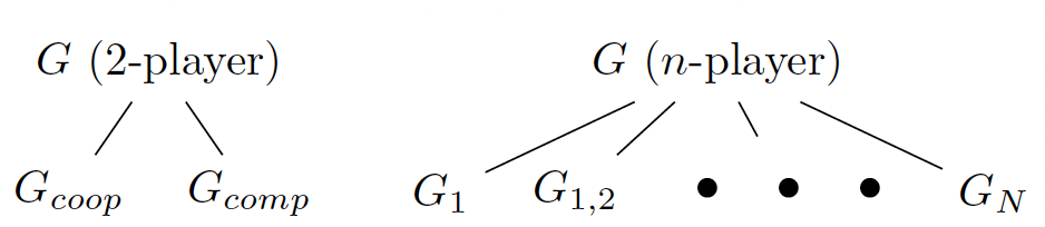
Figure 2: (Right) Illustration of the decomposition of an $n$-player game $G$ into $2^{n}-1$ coalitional games vs. (Left) the Coco decomposition of Kalai and Kalai (2013) for $2$-player games.

Let $G=(U_{1},\ldots,U_{n})$ be an $n$-player, general sum game. Let $\mathcal{V}$ be the set of all coalitions (subsets) of players. For coalition $I\in\mathcal{V}$, we define a game $G_{I}$ as follows: all players of coalition $I$ are identified into one player, who plays against the complement coalition $\bar{I}$. The utility for player $I$ is defined to be $U_{I}=\sum_{j\in I}U_{j}-\sum_{j\notin I}U_{j}$, and the utility for player $\bar{I}$ is defined to be $U_{\bar{I}}=-U_{I}$. Then $G_{I}=(U_{I},U_{\bar{I}})$. Since $G_{I}$ is a two-player, zero-sum game, $\textrm{maxmin}(G_{I})$ is well-defined. The only exception is when $I=N$, the grand coalition, in which case there is only one player. We handle this case separately: $G_{N}$ is the fully cooperative game where all players in $N$ have the same utility function $U_{N}=\sum_{j\in N}U_{j}$.

Intuitively, $\textrm{maxmin}(G_{I})$ quantifies how strong the coalition $I$ is when playing competitively against its complement. Then, we define the HS value for player $i$ to be the average over all coalitions in which player $i$ takes part. Formally, we have

Definition 2.1 (HS computation).

For game $G$, the HS value for player $i$ may be computed as follows: $\text{HS}_{i}(G)=\frac{1}{n}\left(\textrm{maxmax}_{i}(G_{N})+\sum_{I\subsetneqq N:i\in I}\binom{n-1}{|I|-1}^{-1}\textrm{maxmin}_{I}(G_{I})\right).$ Further, define the HS operator on a game to be $\text{HS}(G)=(\text{HS}_{1}(G),\text{HS}_{2}(G),\ldots,\text{HS}_{n}(G))$.

The value $\binom{n-1}{|I|-1}$ is the number of possible coalitions of size $I$ in which player $i$ takes part, which determines the coefficients. Observe that this formula for HS agrees with the $2$-player Coco formula of Kalai and Kalai (2013) when $n=2$.

Example. To illustrate the HS computation, we compute the HS values for a $3$-player adaptation of the 2-player banana game from Section 1. Player 1 is tall and has actions reach and climb. As before, she can obtain $4$ bananas by climbing on a short player and 2 bananas by reaching. Her action set is $A_{1}=\{R,C\}$. Players 2, 3 are short, and can decide to boost Player 1 or not: thus, $A_{2}=A_{3}=\{B,NB\}$. The utility functions are given as follows; below, entry $(a,b,c)$ represents the payoffs for players 1,2,3, respectively.

$$\begin{array}[]{c | cc }\lx@intercol\hfil P1:R\hfil\lx@intercol\\ &P3:B&P3:NB\\ \hline\cr P2:B&(2,0,0)&(2,0,0)\\ P2:NB&(2,0,0)&(2,0,0)\end{array},$$

$$\begin{array}[]{c | cc }\lx@intercol\hfil P1:C\hfil\lx@intercol\\ &P3:B&P3:NB\\ \hline\cr P2:B&(4,0,0)&(4,0,0)\\ P2:NB&(4,0,0)&(0,0,0)\end{array}$$

The HS definition requires that we analyze the two-player zero-sum coalition games; for details, see Appendix A. We compute $\text{HS}(G)=(10/3,1/3,1/3)$. Thus, we see that adding an additional short player to the original 2-player version has resulted in an increased HS value for the tall player from $3$ to $10/3$. This makes sense since the tall player may work with either short player and hence the strategic position of the tall player is better than in the 2-player version. Also, each of the short players receives $1/3$ of a banana.

2.2 Shapley Interpretation and Equivalence to Harsanyi (1963)

In this section, we show that the $n$-player HS computation above is equal to the value of Harsanyi (1963), a modification of the Shapley value . Let $G=(U_{1},\ldots,U_{n})$ be an $n$-player, normal-form game with players $N=\{1,\ldots,n\}$.

Definition 2.2 (Shapley value).

Given function $v:2^{N}\to\mathbb{R}$, with $v(\emptyset)=0$. Then the Shapley value for player $i$ is:

$$s_{i}(G)=\sum_{I\subseteq N:i\in I}\frac{(|I|-1)!(n-|I|)!}{n!}(v(I)-v(\overline{I}))$$

Harsanyi (1963) defined the HS value to be the Shapley value with a particular $v$ function. Let $v(I)$ be defined in the following way: define $G_{I}$ as in Section 2.1; that is, all players of coalition $I$ are identified into one player, who plays against the complement coalition $\bar{I}$. The utility for player $I$ is defined to be $U_{I}=\sum_{j\in I}U_{j}-\sum_{j\notin I}U_{j}$, and the utility for player $\bar{I}$ is defined to be $U_{\bar{I}}=-U_{I}$. Then $G_{I}=(U_{I},U_{\bar{I}})$. Now, consider a Nash equilibrium of $G_{I}$, which gives a probability distribution $p$ over the joint action space $\mathbf{A}$. Then

$$\textrm{maxmin}(G_{I}) =\sum_{\mathbf{a}\in\mathbf{A}}p(\mathbf{a})U_{I}(\mathbf{a})$$

$$=\sum_{\mathbf{a}\in\mathbf{A}}p(\mathbf{a})\left(\sum_{j\in I}U_{j}(\mathbf{a})-\sum_{j\not\in I}U_{j}(\mathbf{a})\right).$$ (1)

Next, given the probability distribution $p$ from the Nash equilibrium, define $v(I)$ as follows: $v(I)=\sum_{\mathbf{a}\in A}p(\mathbf{a})\left(\sum_{j\in I}U_{j}(\mathbf{a})\right)$.

Proposition 2.3.

The modified Shapley value $(s_{1},\ldots,s_{n})$ of Harsanyi (1963) is equal to our computation above; that is, for all $i\in N$, $\text{HS}_{i}(G)=s_{i}(G)$.

Proof.

Since the equilibrium value for a 2-player, zero-sum game is unique (Von Neumann and Morgenstern, 1944), $\textrm{maxmin}(G_{\bar{I}})=-\textrm{maxmin}(G_{I})$, and it follows that $\textrm{maxmin}(G_{I})=v(I)-v(\bar{I})$. Therefore, $\text{HS}_{i}(G)$ is equal to

$$\frac{1}{n}\left(\textrm{maxmax}_{i}(G_{N})+\sum_{I\subsetneqq N:i\in I}\binom{n-1}{|I|-1}^{-1}\textrm{maxmin}_{I}(G_{I})\right)$$

$$=\frac{1}{n}\left((v(N)-v(\emptyset))+\sum_{I\subsetneqq N:i\in I}\binom{n-1}{|I|-1}^{-1}(v(I)-v(\bar{I}))\right)$$

$$=\sum_{I\subseteq N:i\in I}\frac{(|I|-1)!(n-|I|)!}{n!}(v(I)-v(\overline{I}))=s_{i}(G).\qed$$

3 HS Values for Stochastic Games

In this section, we generalize the $n$-player HS definition to general-sum, stochastic games. We provide two approaches to generalize to stochastic games. Both generalizations are well motivated (and in the $2$-player case, they coincide), but surprisingly they are not equal in the case of $n$ players.

Discussion. The generalization in Section 3.1 works by decomposing the original, $n$-player stochastic game into many $2$-player, zero-sum stochastic games. By previous results for fully cooperative and competitive stochastic games (Szepesvári and Littman, 1996) a value function $\mathbf{V}_{I}$ can be defined for each coalition $I\subseteq N$ of players. This definition is well-defined and can be computed using Friend-$Q$ and Minimax-$Q$. These nice properties are why we present it as our main definition.

An alternative approach is given in Section 3.2. This version seeks to define the stochastic HS values for each state using the generalized Bellman equations, in which the normal-form HS computation is used in the definition of the operator $\bigotimes$. This is perhaps the most natural way to generalize to stochastic games, as it is a direct generalization of the Bellman equations for single agent MDPs to use the HS operator – this is the method employed by Sodomka et al. (2013) to generalize the $2$-player HS values to stochastic games. For clarity, we refer to this version as $\text{HS}*$. In fact, in the case of $2$ players, we show that $\mathbf{V}_{\text{HS}}=\mathbf{V}_{\text{HS}*}$, that is, the two generalizations coincide.

Perhaps surprisingly, we show that with more than $2$ players, these approaches differ; that is, the $\mathbf{V}_{\text{HS}}\neq\mathbf{V}_{\text{HS}*}$. This difference is shown on examples in our evaluation in Section 4. Moreover, it is unclear if generalized $Q$ learning with $\bigotimes=\text{HS}*$ (or even value iteration) converges.

3.1 HS Values for Stochastic Games

In this section, we generalize the normal-form HS values to stochastic games. Let $\mathcal{G}=(N,X,\mathbf{A},P,\mathbf{R},\gamma)$ be a general-sum, stochastic game, with set $N$ of $n$ players. We will decompose $\mathcal{G}$ into $2^{n}-1$ stochastic games, one fully cooperative game, and the rest $2$-player, zero-sum games. Each two-player, zero-sum stochastic game will correspond to a coalition of players $I\subseteq N$. Then, we define the HS value function for player $i$ analogously to the normal-form definition in Section 2.1 by summing over the value functions of all coalitions containing player $i$ multiplied by the normalizing coefficients.

Let coalition $I\subseteq N$. From the original $n$-player stochastic game, we identify all players in $I$ as a single player with action space $A_{I}=\bigtimes_{i\in I}A_{i}$; similarly, all players in $\bar{I}=N\setminus I$ are identified into a single player. The utility function of player $I$ is defined as $U_{I}=\sum_{j\in I}R_{j}-\sum_{j\not\in I}R_{j}$; and $U_{\bar{I}}=-U_{I}$. We then consider the stochastic game $\mathcal{G}_{I}=(\{I,\bar{I}\},(A_{I},A_{\bar{I}}),P,(U_{I},U_{\bar{I}}),\gamma)$. Since this is a $2$-player, zero-sum stochastic game, Minimax-$Q$ (Littman, 1994; Szepesvári and Littman, 1996) can be used to calculate the values $V_{I}:X\to\mathbb{R}$ of player $I$ at each state.

Explicitly, let $x\in X$ be an arbitrary state, and let $V:X\to\mathbb{R}$ be an arbitrary value function. For joint action $(a,\bar{a})\in A_{I}\times A_{\bar{I}}$, define $W_{I}(a,\bar{a})=\sum_{y\in X}P(x,a,y)[U_{I}(x,a,y)+\gamma V(y)].$ Define the zero-sum two-player game $H_{x}(V)=(W_{I},-W_{I})$. Then, we define operator $T_{I}(V)$ by

$$[T_{I}(V)](x)=\textrm{maxmin}_{I}(H_{x}(V)).$$

It is convenient to allow the above notation to subsume the case when $I=N$ and the game is fully cooperative, in which case it is a maxmax operator. The generalized Bellman equations for the two-player, zero-sum stochastic game corresponding to coalition $I$ are

$$V(x)=[T_{I}(V)](x),\;\forall x\in X.$$ (2)

It is known that Eq. 2, for the optimal policy in a 2-player, zero-sum stochastic game, admits a unique solution $V_{I}^{*}:X\to\mathbb{R}$ that may be found by value iteration or generalized $Q$-learning (Section 4.2 of Szepesvári and Littman (1996)).

Now that $V_{I}^{*}$ is defined for all $I\subseteq N$, one may use them to define the HS values.

Definition 3.1 (HS values for stochastic game).

Let $\mathcal{G}=(N,X,\mathbf{A},P,\mathbf{R},\gamma)$ be a stochastic game; for each $I\subseteq N$, define $V_{I}^{*}:X\to\mathbb{R}$ as above.

Let $i\in N$. At state $x\in X$, define

$$V_{\text{HS},i}(x)=\frac{1}{n}\sum_{I\subseteq N:i\in I}\binom{n-1}{|I-1|}^{-1}V_{I}^{*}(x),$$ (3)

and $\mathbf{V}_{\text{HS}}=(V_{\text{HS},i})_{i\in N}$.

Remark 3.2.

As in the normal-form definition, when $I=N$, we have a fully cooperative part of the value. Observe that only one of $V_{I}^{*}$, $V^{*}_{N\setminus I}$ must be computed, since $V_{I}^{*}(x)=-V^{*}_{N\setminus I}(x)$ for all $x\in X$.

3.2 $\text{HS}*$ Values for Stochastic Games – An Alternative Approach

In this approach, we use the HS operator for normal-form games (Def. 2.1) in the generalized Bellman equations to define an HS-like value for stochastic games – to distinguish this value, we term it $\text{HS}*$. Let $\mathcal{G}=(N,X,\mathbf{A},P,\mathbf{R},\gamma)$ be a stochastic game.

First, we define an $n$-player, normal-form game at each state $x\in X$. For joint action $\mathbf{a}$ of the players, the game assigns the expected utility for each player according to the reward from the transition and the current value of the resulting state. Formally, let $\mathbf{V}=(V_{1},\ldots,V_{n}):X\to\mathbb{R}^{n}$. Define the utility for player $i$ for joint action $\mathbf{a}$: $U_{i}(x,\mathbf{a},\mathbf{V})=\sum_{y\in X}P(x,\mathbf{a},y)[R_{i}(x,\mathbf{a},y)+\gamma V_{i}(y)],$ and finally define $G_{x}(\mathbf{V})=(U_{1}(x,\cdot,\mathbf{V}),\ldots,U_{n}(x,\cdot,\mathbf{V}))$.

Definition 3.3 (Operator $T$).

Let $\mathcal{B}$ be the space of functions from $X$ to $\mathbb{R}^{n}$. Define operator $T:\mathcal{B}\to\mathcal{B}$ by

$$[T(\mathbf{V})](x)=\textsc{HS}\left(G_{x}(\mathbf{V})\right).$$

Operator $T$ is used to define the generalized Bellman equations.

Definition 3.4 ($\text{HS}*$ values for stochastic game).

The $\text{HS}*$ value $\mathbf{V}_{\text{HS}*}$ is a solution of the following equations.

$$\mathbf{V}(x)=[T(\mathbf{V})](x),\;\forall x\in X.$$ (4)

Remark 3.5.

As discussed above, it is unclear if this definition is well-defined or converges with generalized $Q$ learning or even value iteration. In any event, it does not agree with our definition of $\mathbf{V}_{\text{HS}}$. In Section 4, our implementation of value iteration with operator $T$ converges on every stochastic game tested. This empirical convergence is in contrast with the classical Correlated-$Q$ learning algorithm (Greenwald et al., 2003), which did not converge on most of our games. This empirical convergence leads us to conjecture that $\text{HS}*$ is well defined and can be computed with value iteration.

Proposition 3.6.

If $\mathcal{G}$ is a $2$-player, general-sum stochastic game, $\mathbf{V}_{\text{HS}}=\mathbf{V}_{\text{HS}*}$. In general, $\mathbf{V}_{\text{HS}}\neq\mathbf{V}_{\text{HS}*}$.

Proof.

Let $\mathcal{G}$ be a $2$-player stochastic game. Let $\mathbf{V}=(V_{1},V_{2}):X\to\mathbb{R}^{2}$ be a function. Define $W_{1}(x)=V_{1}(x)-V_{2}(x)$. Next, apply $T$ to $\mathbf{V}$ to get $\widehat{\mathbf{V}}=T(\mathbf{V})$. Now, let $\widehat{W}_{1}(x)=\widehat{V}_{1}(x)-\widehat{V}_{2}(x)$. Then

$$\widehat{W}_{1}(x) =\widehat{V}_{1}(x)-\widehat{V}_{2}(x)$$

$$=\frac{1}{2}[(\textrm{maxmin}_{1}(G_{x,1}(\mathbf{V}))+\textrm{maxmax}_{1}(G_{x,1,2}(\mathbf{V})))$$

$$\;\;-(\textrm{maxmin}_{2}(G_{x,2}(\mathbf{V}))+\textrm{maxmax}_{2}(G_{x,1,2}(\mathbf{V})))$$

$$=\textrm{maxmin}_{1}(G_{x,1}(\mathbf{V}))$$

$$=T_{1}(V_{1}-V_{2})(x)=T_{1}(W_{1})(x),$$

where $T_{1}$ is the operator defined in Section 3.1. Therefore, as $T$ is applied repeatedly, $W_{1}$ converges to $V_{1}^{*}$ as defined in Section 3.1.

Similarly, if $W_{2}=V_{2}-V_{1}$; and $W_{1,2}=V_{1}+V_{2}$, we have that $W_{2}\to V_{2}^{*}$ and $W_{1,2}\to V_{1,2}^{*}$ as $T$ is iteratively applied. Therefore, $V_{1}=\frac{1}{2}(W_{1,2}+W_{1})$ and $V_{2}=\frac{1}{2}(W_{1,2}+W_{2})$ both converge, precisely to $(V_{\text{HS},1},V_{\text{HS},2})=\mathbf{V}_{\text{HS}}$, which completes the proof.

Examples that show $\mathbf{V}_{\text{HS}}\neq\mathbf{V}_{\text{HS}*}$ when $n>2$ are provided in Section 4. ∎

4 Empirical Evaluation

In this section, we learn $\mathbf{V}_{\text{HS}},\mathbf{V}_{\text{HS}*}$ and extract the resulting policies and side payments on a standard test suite of grid games generalized to more than two players. As a baseline, we also implement Correlated-$Q$ (Greenwald et al., 2003) with the utilitarian objective to select a correlated equilibrium. All learning is done with value iteration, since the environment is known. Source code to reproduce the results is available in the supplementary material.

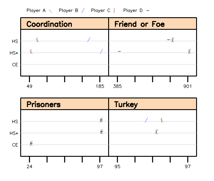
Figure 3: The strategic value for each player in each game, as computed by the corresponding algorithm.

Summary of results. We find that both HS and $\text{HS}*$ learn sensible assessments of the strategic strength of each player and enable maximizing the overall combined score while preserving the competitive nature of the game. This is achieved through side payments that encourage other players to act in ways that may not be immediately advantageous. Usually, HS and $\text{HS}*$ agree on at least the relative strength of the players, although this is not always the case (see Fig. 3). Frequently, they disagree on the nominal strength of the players. Surprisingly, Correlated-$Q$ did not converge on most of our games, with the exception of Prisoners.

We find that the side payments at each state transition learned by $\text{HS}*$ agree better with our intuition (see the discussion below) – this is likely because the definition $\text{HS}*$ is in terms of the (normal-form) HS value at each state transition. For HS, the side payments make more sense on a policy level.

In symmetric games like Prisoners, both HS and $\text{HS}*$ find a series of side payments that ultimately result in symmetric values for all players. In games like Coordination, where one player has a significant advantage from the start, both algorithms learn a final value that is proportionate to the players’ starting strengths. Additionally, in Friend-or-Foe, we see a large nominal disagreement between HS and $\text{HS}*$ about the strength of the weaker player.

4.1 Grid Games

In Grid games, players compete on a grid of $m\times n$ squares. Each square can be occupied by at most one player. Each player has a designated starting square and a set of individual and shared goal squares where rewards are received. The players can observe the positions of themselves and other players on the grid. Additionally, there are walls and semi-walls that impede movement. During each round, all players simultaneously choose an action from the options of moving up, down, left, right, or sticking in place. Each move incurs a step cost of $-1.0$, even when the player is unable to move as intended. Sticking incurs a step cost of $-0.1$.

When a player selects a move without obstacles, they move in the chosen direction. If a player tries to move through a wall or to a square already occupied by a sticking player, they stay in their current square. If a player attempts to move through a semi-wall, they have a 50% chance of doing so, otherwise they stay in their current location. If two players try to move into the same square, one is randomly selected to move and the other stays in their current location.

The game concludes when one of the players reaches a goal square, which has a positive reward assigned to it. If multiple players reach their goal squares simultaneously, they all receive rewards. In our experiments, unless otherwise stated, the rewards for reaching the goal are set to 100, the cost of taking a step is -1, and the reward for staying in the same place is -0.1. The discount factor $\gamma$ is set to 1 for ease of interpretability.

Agents are represented on the grid as A, B, C, and D. The goal squares for each agent are drawn with unique directional lines. In the case where agents have a shared goal, all sets of lines will be displayed. The path taken by the agent is shown as a sequence of arrows pointing from the agent’s current square to its next. Each time an agent moves to a new square, the corresponding arrow of the path is labeled with the time step. A ”stick” and failed actions are illustrated as another time label in the same square. The side payments and total trajectory values for each agent are displayed below the game, with positive values indicating an agent received a payment and negative values indicating that the agent made a payment.

4.2 Results

In this section, we compare the learned policies and side payments on specific examples of grid games: Prisoners; Friend-or-Foe, Coordination; and Turkey. All of these grid games are generalizations of commonly used $2$-player grid games (Hu and Wellman, 2003; Greenwald et al., 2003; Sodomka et al., 2013) to more than $2$ players.

Coordination. In the Coordination game (as illustrated in Fig. 4), Players A, B, and C each have their own goals they need to reach without colliding by coordinating their moves across the grid. Notice that Players $A$ and $C$ are symmetric, but player $B$ is closer to her goal than the other players. Therefore, one would expect that the strategic value of Player $B$ is stronger than the others; and that therefore, Players A and C should pay Player B to allow them to make it to their respective goals.

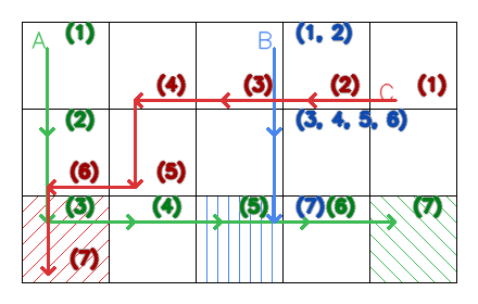
State	HS	HS*
1	(-0.1, -0.2, 0.3)	(-7.6, 15.2, -7.6)
2	(0.2, -0.3, 0.1)	(-5.0, -7.9, 12.9)
3	(-16.3, 32.1, -15.8)	(-30.4, 52.2, -21.8)
4	(-16.2, 32.7, -16.6)	(-13.7, 54.0, -40.3)
5	(0.5, -0.4, -0.0)	(12.4, -25.1, 12.7)
6	(0.0, -0.0, -0.0)	(0.0, 0.0, 0.0)
V	(62.0, 161.6, 62.0)	(49.8, 185.9, 49.8)
SP	(-32.0, 64.0, -32.0)	(-44.2, 88.3, -44.2)

Figure 4: A learned HS and $\text{HS}*$ trajectory in Coordination, with the side payments as computed by each algorithm. The value of the trajectory is indicated by (V) and the total side payments by (SP).

In Fig. 4, we show the trajectory learned by the algorithms. Also, in the table of Fig. 4, we show the values for the side payments made at each step along the trajectory, as well as the total value (V) and the total side payments (SP). Both $\mathbf{V}_{\text{HS}}$ and $\mathbf{V}_{\text{HS}*}$ agree with the above intuition, while Correlated-$Q$ did not converge. Player B is the strongest, and Players A and C have to pay Player B to stick while they coordinate their passing. The $\text{HS}*$ side payments shown in the table agree better with our intuition. For example, in State 1, why should Player B pay the other players to stick, when it is against his immediate self-interest? $\text{HS}*$ agrees with our intuition by having the other players pay Player B to stick.

Additionally, HS and $\text{HS}*$ disagree on just how strong Player B is. While HS and $\text{HS}*$ often agree on the relative strength of the players, they do not always. For example, at State 5, there is a strong disagreement about the strength of Player B: in this state, Player A is occupying the goal of Player B. The HS value considers all players to be roughly equal, since Player A cannot proceed to his own goal without moving off of the goal of Player B. However, the $\text{HS}*$ value takes the threat of Players A and C working together much more seriously.

Prisoners. The game depicted in Fig. 6 is based on the classic normal-form Prisoners’ Dilemma game, with each agent having her own goal located at the end of her respective hallway and a shared goal in the center. In this grid game, moving towards the shared goal (defecting) is the rational strategy for each agent If any agent chooses to move towards the shared goal, the others also prefer to move towards it to potentially win the tiebreaker. However, if agents cooperate and move towards their own goals, they all can receive a higher expected value.

The side payments table in Fig. 6 illustrates the payments exchanged during the players’ progression. Player D strategically pays Players A, B, and C to move away from the shared objective, gaining a significant advantage over them. As a result, A, B, and C become vulnerable and are forced to pay Player D to stay in place temporarily, in order to position themselves to reach their individual goals. Once each player is in a position to score, no further side payments are made among them. Notably, HS and $\text{HS}*$ agree exactly on the values of the players at each state in this game, as well as the side payments. The Correlated-$Q$ policy has each player choose their rational strategy of attempting to move into the shared goal, resulting in a win with a probability of 0.25 and an expected value of 24.0, which is significantly lower than the HS value.

Turkey. The game shown in Figure 7 involves agents with individual goals located three steps below their starting positions. Semi-walls, represented by thick dashed lines, are placed between the agent and its goal, with a probability of 0.5 for success if an agent attempts to pass through it. Additionally, there are two shared goals placed three spaces from each pair of agents.

For this game, the trajectory corresponding to the $\text{HS},\text{HS}*$ policy is not deterministic, but depends on what happens when a player attempts to pass through a semi-wall. In the depicted trajectory in Fig. 7, Player A attempts to pass through the semi-wall and was unsuccessful. They took this risky action because they were paid by both Players B and C to do so, which allowed them to move around their own semi-wall with guaranteed success. Once Player A has passed through the semi-wall, they coerced the cooperation of Players B and C via a payment to stick while A gets into position for a score.

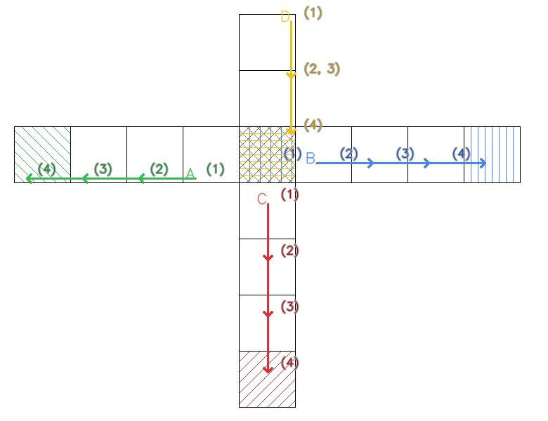
State	HS
1	(116.3, 116.3, 116.3, -349.0)
2	(-332.8, -332.8, -332.8, 998.4)
3	(0.0, 0.0, 0.0, 0.0)
V	(780.6, 780.6, 780.6, 747.2)
SP	(-216.4, -216.4, -216.4, 649.3)

State	HS*
1	(236.8, 236.8, 236.8, -710.5)
2	(-332.8, -332.8, -332.8, 998.4)
3	(0.0, 0.0, 0.0, 0.0)
V	(901.0, 901.0, 901.0, 385.8)
SP	(-96.0, -96.0, -96.0, 287.9)

Figure 5: A Friend-or-Foe trajectory with side payments.

Friend-or-Foe. The game of Friend-or-Foe, depicted in Figure 5, has a weak player (Player D) who starts two steps away from a shared goal with reward $100$. The other players start one step from the shared goal, but have their own goals worth $1000$ three steps away. If the other players try to move to their high-value goals, the weaker player can act as a spoiler (which is also in her self interest) by moving to the shared goal and ending the game.

Both HS and $\text{HS}*$ determine that Player D should pay the others to move away from the shared goal, but there is a large disagreement about the amount of the payment. $\text{HS}*$ assigns a larger payment since Player D is powerless in the normal-form game at the first state. After the first state, Player D is in a stronger position than the others and HS and $\text{HS}*$ agree on the strategic value on the rest of the trajectory.

5 Conclusion and Future Work

In this paper, we provide a simple formula to compute the Harsanyi-Shapley value of a player (Harsanyi, 1963), which generalizes the $2$-player Coco formula of (Kalai and Kalai, 2013). We then generalize our computation to stochastic games to achieve a well-defined HS value that is learnable with generalized $Q$ learning. We define a second notion, $\text{HS}*$, based upon generalized Bellman equations. Although we did not show that the $\text{HS}*$ values are well-defined or learnable, we were able to learn them on all of our example games. Empirically, they provide a viable alternative the HS value on stochastic games that may provide a more interpretable side payment at each step. Future work includes determining whether $\text{HS}*$ is theoretically learnable and developing more scalable algorithms to learn the HS and $\text{HS}*$ value.

Appendix A Computation of $3$-Player Banana Example

Case $I=\{1\}$, $\bar{I}=\{2,3\}$. Then the payoff matrix for player $I$ is

$$R=\begin{array}[]{cc | cccc }&\lx@intercol\hfil\bar{I}\hfil\lx@intercol\\ &&(B,B)&(B,NB)&(NB,B)&(NB,NB)\\ \hline\cr&R&2&2&2&2\\ \smash{\raisebox{3.60004pt}{$I$}}&C&4&4&4&0\end{array}$$

The payoff matrix for $\bar{I}$ is $-R$. Then $\textrm{maxmin}(G_{I})=\textrm{maxmin}(R)=2$, and hence $\textrm{maxmin}(G_{\bar{I}})=-2$.

Case $I=\{2\}$, $\bar{I}=\{1,3\}$. Then the payoff matrix for player $I$ is

$$R=\begin{array}[]{cc | cccc }&\lx@intercol\hfil\bar{I}\hfil\lx@intercol\\ &&(R,B)&(R,NB)&(C,B)&(C,NB)\\ \hline\cr&B&-2&-2&-4&-4\\ \smash{\raisebox{3.60004pt}{$I$}}&NB&-2&-2&-4&0\end{array}$$

The payoff matrix for $\bar{I}$ is $-R$. Then $\textrm{maxmin}(G_{I})=\textrm{maxmin}(R)=-4$, and $\textrm{maxmin}(G_{\bar{I}})=4$.

Case $I=\{3\}$, $\bar{I}=\{1,2\}$. This computation is the same as the preceding case, giving $\textrm{maxmin}(G_{I})=\textrm{maxmin}(R)=-4$, and $\textrm{maxmin}(G_{\bar{I}})=4$.

Case $I=\{1,2,3\}$. Then $\textrm{maxmax}(G_{I})=\max_{a\in A}(R^{1}(a)+R^{2}(a)+R^{3}(a))=4$.

Having computed the maxmin for each coalitional game, we now compute the HS values: $\text{HS}_{1}=\frac{1}{3}(\textrm{val}(\{1\})+\frac{1}{2}(\textrm{val}(\{1,2\})+\textrm{val}(\{1,3\}))+\textrm{val}(\{1,2,3\}))=10/3,$ $\text{HS}_{2}=\frac{1}{3}(\textrm{val}(\{2\})+\frac{1}{2}(\textrm{val}(\{2,3\})+\textrm{val}(\{1,2\}))+\textrm{val}(\{1,2,3\}))=1/3,$ and $\text{HS}_{3}=\text{HS}_{2}=1/3$.

Appendix B Additional Empirical Results

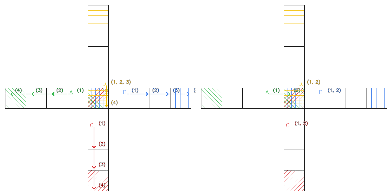
State	HS	HS*
1	(33.2, 33.2, 33.2, -99.7)	(33.2, 33.2, 33.2, -99.7)
2	(-32.8, -32.8, -32.8, 98.4)	(-32.8, -32.8, -32.8, 98.4)
3	(0.0, 0.0, 0.0, -0.0)	(0.0, 0.0, 0.0, 0.0)
V	(97.5, 97.5, 97.5, 97.5)	(97.5, 97.5, 97.5, 97.5)
SP	(0.5, 0.5, 0.5, -1.4)	(0.5, 0.5, 0.5, -1.4)

Figure 6: Prisoners. Top: A trajectory of $\text{HS},\text{HS}*$ (Left) and Correlated-$Q$ (Right). Bottom: Side payments for the trajectory in top left.

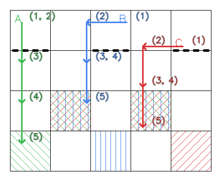
State	HS	HS*
1	(75.4, -37.4, -36.8)	(65.9, -32.3, -32.3)
2	(-9.1, 3.9, 3.9)	(0.2, -0.7, -0.7)
3	(-65.5, 32.8, 32.8)	(-65.5, 32.7, 32.7)
4	(0.0, 0.0, 0.0)	(0.0, -0.0, -0.0)
V	(96.8, 96.2, 96.8)	(96.6, 96.6, 96.6)
SP	(0.8, -0.7, -0.1)	(0.6, -0.3, -0.3)

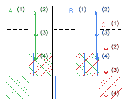
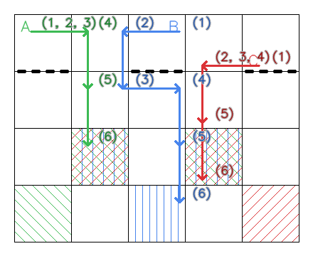
Figure 7: Multiple trajectories generated by the HS and $\text{HS}*$ policy in the Turkey Game. The first (Top) shows Player A attempting the semi-wall, the second (Bottom-Left) shows Player C moving through the semi-wall. The final trajectory (Bottom-Right), shows Player B moving out of the way of Player A for a guaranteed movement.

References

- Casgrain et al. (2022) Philippe Casgrain, Brian Ning, and Sebastian Jaimungal. Deep Q-Learning for Nash Equilibria: Nash-DQN. Applied Mathematical Finance, 29(1):62–78, January 2022.
- Daskalakis et al. (2009) Constantinos Daskalakis, Paul W. Goldberg, and Christos H. Papadimitriou. The Complexity of Computing a Nash Equilibrium. SIAM Journal on Computing, 39(1):195–259, January 2009.
- Deng et al. (2021) Xiaotie Deng, Yuhao Li, David Henry Mguni, Jun Wang, and Yaodong Yang. On the Complexity of Computing Markov Perfect Equilibrium in General-Sum Stochastic Games, September 2021.
- Greenwald et al. (2003) Amy Greenwald, Keith Hall, and Roberto Serrano. Correlated Q-learning. In ICML, volume 3, pages 242–249, 2003.
- Gronauer and Diepold (2022) Sven Gronauer and Klaus Diepold. Multi-agent deep reinforcement learning: A survey. Artificial Intelligence Review, 55(2):895–943, 2022.
- Harsanyi (1963) John C. Harsanyi. A Simplified Bargaining Model for the n-Person Cooperative Game. International Economic Review, 4(2):194–220, 1963.
- Hernandez-Leal et al. (2019) Pablo Hernandez-Leal, Bilal Kartal, and Matthew E. Taylor. A survey and critique of multiagent deep reinforcement learning. Autonomous Agents and Multi-Agent Systems, 33(6):750–797, November 2019.
- Hu and Wellman (2003) Junling Hu and Michael P. Wellman. Nash Q-learning for general-sum stochastic games. Journal of machine learning research, 4(Nov):1039–1069, 2003.
- Hughes et al. (2020) Edward Hughes, Thomas W. Anthony, Tom Eccles, Joel Z. Leibo, David Balduzzi, and Yoram Bachrach. Learning to Resolve Alliance Dilemmas in Many-Player Zero-Sum Games, February 2020.
- Kalai and Kalai (2013) Adam Kalai and Ehud Kalai. Cooperation in Strategic Games Revisited*. The Quarterly Journal of Economics, 128(2):917–966, May 2013.
- Kalai and Rosenthal (1978) E. Kalai and R. W. Rosenthal. Arbitration of two-party disputes under ignorance. International Journal of Game Theory, 7(2):65–72, June 1978.
- Kohlberg and Neyman (2021) Elon Kohlberg and Abraham Neyman. Cooperative strategic games. Theoretical Economics, 16(3):825–851, 2021.
- Littman (1994) Michael L. Littman. Markov games as a framework for multi-agent reinforcement learning. In William W. Cohen and Haym Hirsh, editors, Machine Learning Proceedings 1994, pages 157–163. Morgan Kaufmann, San Francisco (CA), January 1994.
- Littman (2001) Michael L. Littman. Friend-or-foe Q-learning in general-sum games. In ICML, volume 1, pages 322–328, 2001.
- Mao and Başar (2022) Weichao Mao and Tamer Başar. Provably Efficient Reinforcement Learning in Decentralized General-Sum Markov Games. Dynamic Games and Applications, January 2022.
- Mao et al. (2022) Weichao Mao, Lin Yang, Kaiqing Zhang, and Tamer Basar. On improving model-free algorithms for decentralized multi-agent reinforcement learning. In International Conference on Machine Learning, pages 15007–15049. PMLR, 2022.
- Nash (1953) John Nash. Two-Person Cooperative Games. Econometrica, 21(1):128–140, 1953.
- Shoham et al. (2007) Yoav Shoham, Rob Powers, and Trond Grenager. If multi-agent learning is the answer, what is the question? Artificial intelligence, 171(7):365–377, 2007.
- Sodomka et al. (2013) Eric Sodomka, Elizabeth Hilliard, Michael Littman, and Amy Greenwald. Coco-Q: Learning in Stochastic Games with Side Payments. In Proceedings of the 30th International Conference on Machine Learning, pages 1471–1479. PMLR, May 2013.
- Song et al. (2021) Ziang Song, Song Mei, and Yu Bai. When Can We Learn General-Sum Markov Games with a Large Number of Players Sample-Efficiently? arXiv preprint arXiv:2110.04184, 2021.
- Sun et al. (2022) Yu Sun, Jun Lai, Lei Cao, Xiliang Chen, Zhixiong Xu, Zhen Lian, and Huijin Fan. A Friend-or-Foe framework for multi-agent reinforcement learning policy generation in mixing cooperative–competitive scenarios. Transactions of the Institute of Measurement and Control, page 01423312221077755, 2022.
- Szepesvári and Littman (1996) Csaba Szepesvári and Michael L. Littman. Generalized markov decision processes: Dynamic-programming and reinforcement-learning algorithms. Technical Report, (November):1–54, 1996.
- Tian et al. (2021) Yi Tian, Yuanhao Wang, Tiancheng Yu, and Suvrit Sra. Online learning in unknown markov games. In International Conference on Machine Learning, pages 10279–10288. PMLR, 2021.
- Von Neumann and Morgenstern (1944) J. Von Neumann and O. Morgenstern. Theory of Games and Economic Behavior. Theory of Games and Economic Behavior. Princeton University Press, Princeton, NJ, US, 1944.
- Wang et al. (2019) Jane X. Wang, Edward Hughes, Chrisantha Fernando, Wojciech M. Czarnecki, Edgar A. Duenez-Guzman, and Joel Z. Leibo. Evolving intrinsic motivations for altruistic behavior, March 2019.
- Watkins and Dayan (1992) Christopher J. C. H. Watkins and Peter Dayan. Q-learning. Machine Learning, 8(3):279–292, May 1992.
- Xie et al. (2020) Qiaomin Xie, Yudong Chen, Zhaoran Wang, and Zhuoran Yang. Learning zero-sum simultaneous-move markov games using function approximation and correlated equilibrium. In Conference on Learning Theory, pages 3674–3682. PMLR, 2020.
- Yang et al. (2020) Jiachen Yang, Ang Li, Mehrdad Farajtabar, Peter Sunehag, Edward Hughes, and Hongyuan Zha. Learning to Incentivize Other Learning Agents. In Advances in Neural Information Processing Systems, volume 33, pages 15208–15219. Curran Associates, Inc., 2020.
- Yu et al. (2022) Chao Yu, Akash Velu, Eugene Vinitsky, Jiaxuan Gao, Yu Wang, Alexandre Bayen, and Yi Wu. The Surprising Effectiveness of PPO in Cooperative, Multi-Agent Games, November 2022.
- Zhang et al. (2020) Kaiqing Zhang, Sham Kakade, Tamer Basar, and Lin Yang. Model-Based Multi-Agent RL in Zero-Sum Markov Games with Near-Optimal Sample Complexity. In Advances in Neural Information Processing Systems, volume 33, pages 1166–1178. Curran Associates, Inc., 2020.