Layer separation of the 3D incompressible Navier–Stokes equation in a bounded domain

Abstract.

We provide an unconditional $L^{2}$ upper bound for the boundary layer separation of Leray–Hopf solutions in a smooth bounded domain. By layer separation, we mean the discrepancy between a (turbulent) low-viscosity Leray–Hopf solution $u^{\nu}$ and a fixed (laminar) regular Euler solution $\bar{u}$ with similar initial conditions and body force. We show an asymptotic upper bound $C\|\bar{u}\|_{L^{\infty}}^{3}T$ on the layer separation, anomalous dissipation, and the work done by friction, which implies the drag coefficient of any object is bounded. This extends the previous result when the Euler solution is a regular shear in a finite channel. The key estimate is to control the boundary vorticity in a way that does not degenerate in the vanishing viscosity limit.

1. Introduction

Let $T>0$ and let $\Omega\subset\mathbb{R}^{3}$ be a smooth bounded domain. Given a smooth solution $\bar{u}:(0,T)\times\Omega\to\mathbb{R}^{3}$ to the Euler equation with impermeability boundary condition $\bar{u}\bigr{\rvert}_{\partial\Omega}\cdot n=0$ and a regular external force $\bar{f}:(0,T)\times\Omega\to\mathbb{R}^{3}$:

($$\mathrm{EE} \partial_{t}\bar{u}+\bar{u}\cdot\nabla\bar{u}+\nabla\bar{P} =\bar{f} \operatorname{div}\bar{u} =0 \text{ in }\Omega,$$)

we estimate the $L^{2}(\Omega)$ difference at time $T$ between $\bar{u}$ and any Leray–Hopf weak solution $u^{\nu}:(0,T)\times\Omega\to\mathbb{R}^{3}$ to the Navier–Stokes equation with kinematic viscosity $\nu>0$, body force $f^{\nu}\in L^{1}(0,T;L^{2}(\Omega))$, and non-slip boundary condition $u^{\nu}\bigr{\rvert}_{\partial\Omega}=0$:

($$\mathrm{NSE}_{\nu} \partial_{t}u^{\nu}+u^{\nu}\cdot\nabla u^{\nu}+\nabla P^{\nu} =\nu\Delta u^{\nu}+f^{\nu} \operatorname{div}u^{\nu} =0 \text{ in }\Omega.$$)

By Leray–Hopf solution, we mean distributional solutions in the space $u^{\nu}\in C_{\mathrm{w}}(0,T;L^{2}(\Omega))\cap L^{2}(0,T;H^{1}(\Omega))$ satisfying the following energy inequality for every $T^{\prime}\in[0,T]$:

(1) $$\frac{1}{2}\left\lVert u^{\nu}\right\rVert_{L^{2}(\Omega)}^{2}(T^{\prime})+\int_{0}^{T^{\prime}}\int_{\Omega}\nu|\nabla u^{\nu}|^{2}\mathop{\kern 0.0pt\mathrm{d}}\!{}x\mathop{\kern 0.0pt\mathrm{d}}\!{}t$$

$$\qquad\leq\frac{1}{2}\left\lVert u\right\rVert_{L^{2}(\Omega)}^{2}(0)+\int_{0}^{T^{\prime}}\int_{\Omega}u^{\nu}\cdot f^{\nu}\mathop{\kern 0.0pt\mathrm{d}}\!{}x\mathop{\kern 0.0pt\mathrm{d}}\!{}t.$$

One of the fundamental questions in fluid dynamics is whether ideal fluids, governed by the Euler equation, can be used to model viscous fluids with sufficiently small viscosity $\nu$. This can be formulated as the so-called inviscid limit problem, which questions whether the following limit of layer separation is zero:

$$\operatorname{LS}(\bar{u}):=\limsup_{\nu\to 0}\left\{\left\lVert u^{\nu}-\bar{u}\right\rVert_{L^{2}(\Omega)}^{2}(T):\begin{matrix}u^{\nu}(0)\to\bar{u}(0)\text{ in }L^{2}(\Omega)\\ f^{\nu}\to\bar{f}\text{ in }L^{1}(0,T;L^{2}(\Omega))\end{matrix}\right\}.$$

To the best of our knowledge, this question remains open for Leray–Hopf solutions, even for dimension 2.

This paper aims to provide the following unconditional upper bound for layer separation.

Theorem 1.

There exists a universal constant $C>0$ such that the following holds. Let $T>0$ and let $\Omega\subset\mathbb{R}^{3}$ be a domain with compact, smooth boundary satisfying Assumption 1. Let $\bar{u}$ be a regular solution of ($\mathrm{EE}$) with a regular force $\bar{f}$. Let $u^{\nu}$ be a family of Leray–Hopf weak solutions to the Navier–Stokes equation ($\mathrm{NSE}_{\nu}$) with force $f^{\nu}\in L^{1}(0,T;L^{2}(\Omega))$. Then the layer separation is bounded by

$$\operatorname{LS}(\bar{u})\leq CA^{3}T|\partial\Omega|\exp\left(2\int_{0}^{T}\left\lVert D\bar{u}(t)\right\rVert_{L^{\infty}(\Omega)}\mathop{\kern 0.0pt\mathrm{d}}\!{}t\right),$$

where $A=\left\lVert\bar{u}\right\rVert_{L^{\infty}((0,T)\times\partial\Omega)}$ is the maximum boundary velocity of the Euler solution, and $D\bar{u}=\frac{1}{2}(\nabla\bar{u}+\nabla\bar{u}^{\top})$ is the symmetric velocity gradient, also known as the rate-of-strain tensor.

Assumption 1 will be discussed in Section 2.3. It guarantees that the boundary $\partial\Omega$, as a compact manifold, can be triangularized in a uniform way. We conjecture this assumption should be satisfied by all smooth domains.

We remark that the Lipschitz norm of $\bar{u}$ measures only in the interior of $\Omega$, so $\bar{u}$ can be nonzero on the boundary, allowing shear solutions. Indeed, if $\bar{u}$ vanishes on the boundary, then $A=0$ and $\operatorname{LS}(\bar{u})=0$, which can also be verified by elementary computation.

This result is a generalization of the previous work by the authors [VY21] which studied the setting when $\bar{u}$ is a static shear flow in a finite channel without force.

1.1. Literature review

Boundary layer and the inviscid limit problem

The gap between the Euler solution $\bar{u}$ and the low-viscosity Navier–Stokes solution $u^{\nu}$ is due to the “boundary layer”, which refers to a thin layer of fluid near the boundary $\partial\Omega$ that exhibits instability and turbulent structure, in contrast with the regular Euler solution $\bar{u}$ whose behavior near the boundary is predicted to be laminar. This has been observed from physical experiments [LKHM12] and numerical simulations [Dec18]. Via Hilbert expansion, Prandtl [Pra04] conducted an asymptotic analysis of the Navier–Stokes system near the boundary and suggested that the turbulent structure is supported in a boundary layer of width $O(\sqrt{\nu})$. Even though the width of the boundary layer converges to zero in the inviscid limit, it is unclear whether the energy inside the boundary layer always converges to zero. In fact, the Prandtl layer with a simple shear background flow could be ill-posed. [Gre00, E00, GVD10, GVN12]

An important positive result for the inviscid limit to hold is the celebrated work of Kato [Kat84], where he proved $\operatorname{LS}(\bar{u})=0$ if the energy dissipation in a boundary layer of width $\delta=c\nu$ vanishes.

Theorem A (Kato’s Criterion [Kat84]).

Let $\mathcal{U}_{\delta}(\partial\Omega,\Omega)$ be the $\delta$-tubular neighborhood of $\partial\Omega$ in $\Omega$ with $\delta=c\nu$ for some $c>0$. If the following limit holds:

(2) $$\lim_{\nu\to 0}\int_{0}^{T}\int_{\mathcal{U}_{\delta}(\partial\Omega,\Omega)}\nu\left\lvert\nabla u^{\nu}\right\rvert^{2}\mathop{\kern 0.0pt\mathrm{d}}\!{}x\mathop{\kern 0.0pt\mathrm{d}}\!{}t=0,$$

then $\operatorname{LS}(\bar{u})=0$.

Notice that this width is thinner than the Prandtl layer. This indicates that the inviscid limit fails only when the velocity gradient near the boundary has order $\nabla u^{\nu}\sim O(\nu^{-1})$. There have also been unconditional results for the inviscid limit to hold when the solution and the domain enjoy additional structure, for instance, analyticity or symmetry ([Mae14, MM18, FTZ18]).

Nonuniqueness and anomalous dissipation

One important piece of theoretical evidence that suggests the inviscid limit may fail for Leray–Hopf solutions is the nonuniqueness. The recent work of Albritton, Brúe and Colombo [ABC22b, ABC22a] exhibits the nonuniqueness of Leray–Hopf solutions for the forced Navier–Stokes equation. Their construction is based on self-similar solutions [JS15] and Euler instability [Vis18a, Vis18b, ABC⁺21]. Moreover, at the Euler level, even near a constant plug flow $\bar{u}=Ae_{1}$, Széklyhidi [Szé11, VY21] constructed nonunique Euler solutions $\tilde{u}$ using convex integrations with a layer separation of

$$\left\lVert\tilde{u}(T)-\bar{u}\right\rVert_{L^{2}(\Omega)}^{2}=CA^{3}T.$$

Note that this rate is consistent with our upper bound of layer separation. Using convex integration or self-similar solutions, there has been an extensive amount of work in the study of the nonuniqueness of the Euler and the Navier–Stokes equations in the past decades [BDLSV19, BV19, DLS10, Ise18].

Moreover, the layer separation is closely related to anomalous dissipation, which we define under our context as

$$\operatorname{AD}(\bar{u}):=\limsup_{\nu\to 0}\left\{\int_{0}^{T}\int_{\Omega}\nu|\nabla u^{\nu}|^{2}\mathop{\kern 0.0pt\mathrm{d}}\!{}x\mathop{\kern 0.0pt\mathrm{d}}\!{}t:\begin{matrix}u^{\nu}(0)\to\bar{u}(0)\text{ in }L^{2}(\Omega)\\ f^{\nu}\to\bar{f}\text{ in }L^{1}(0,T;L^{2}(\Omega))\end{matrix}\right\}.$$

Kato’s criterion shows that if $\operatorname{AD}(\bar{u})=0$ then $\operatorname{LS}(\bar{u})=0$. It is also straightforward to see from the energy inequality (1) that $\operatorname{LS}(\bar{u})=0$ would imply $\operatorname{AD}(\bar{u})=0$ as well. From this perspective, the validity of the inviscid limit is equivalent to whether the Kolmogorov’s zeroth law of turbulence [Kol41a, Kol41c, Kol41b] can hold in a neighborhood of regular solution $\bar{u}$. In the absence of boundary, Brué and De Lellis [BDL23] constructed examples of classical solutions to the forced Navier–Stokes equation with positive anomalous dissipation. However, both the nonunique Leray–Hopf solutions in [ABC22b] and the anomalous dissipation of [BDL23] are away from a smooth Euler solution, so they do not fall into the scope of this paper. Nevertheless, we provide the same unconditional bound on the limiting energy dissipation as well.

Corollary 1.

Under the same assumptions of Theorem 1, the anomalous dissipation is also bounded by

$$\operatorname{AD}(\bar{u})\leq CA^{3}T|\partial\Omega|\exp\left(2\int_{0}^{T}\left\lVert D\bar{u}(t)\right\rVert_{L^{\infty}(\Omega)}\mathop{\kern 0.0pt\mathrm{d}}\!{}t\right).$$

The drag force and the d’Alembert’s paradox

The crucial term when estimating layer separation and anomalous dissipation is the work done by the friction on the boundary. It is easy to see that the validity of the inviscid limit is equivalent to the vanishing of the work of the drag force (friction):

$$\mathrm{W}_{\text{drag}}(\bar{u}):=\limsup_{\nu\to 0}\left\{\nu\int_{(0,T)\times\partial\Omega}\partial_{n}u^{\nu}\cdot\bar{u}\mathop{\kern 0.0pt\mathrm{d}}\!{}x^{\prime}\mathop{\kern 0.0pt\mathrm{d}}\!{}t:\begin{matrix}u^{\nu}(0)\to\bar{u}(0)\text{ in }L^{2}(\Omega)\\ f^{\nu}\to\bar{f}\text{ in }L^{1}(0,T;L^{2}(\Omega))\end{matrix}\right\},$$

where $\partial_{n}u^{\nu}\cdot\bar{u}=\omega^{\nu}\cdot(n\times\bar{u})$ on the boundary $\partial\Omega$. The question of whether $\mathrm{W}_{\text{drag}}(\bar{u})=0$ is the well-known d’Alembert’s paradox: in a perfectly ideal fluid, there is no drag force; but if the drag force vanishes in the inviscid limit, birds cannot fly in the air because there is little lift.

Using energy inequality and Grönwall inequality, it is easy to see that

(3) $$\operatorname{LS}(\bar{u})+\operatorname{AD}(\bar{u})\leq\mathrm{W}_{\text{drag}}(\bar{u})\exp\left(2\int_{0}^{T}\left\lVert D\bar{u}\right\rVert_{L^{\infty}(\Omega)}\mathop{\kern 0.0pt\mathrm{d}}\!{}t\right).$$

Hence, measuring the layer separation and anomalous dissipation relies on the estimation of boundary vorticity $\omega^{\nu}$. We will provide a uniform bound in $L^{\frac{3}{2}}$ weak space in the Theorem 3, using the energy dissipation in the Kato’s layer. As a consequence of this vorticity estimate, we can control the total work of drag force asymptotically by

$$\mathrm{W}_{\text{drag}}(\bar{u})\leq C\left\lVert\bar{u}\right\rVert_{L^{3,1}((0,T)\times\partial\Omega)}^{\frac{1}{3}}\operatorname{AD}_{c\nu}(\bar{u})^{\frac{2}{3}}\leq CA(T|\partial\Omega|)^{\frac{1}{3}}\operatorname{AD}_{c\nu}(\bar{u})^{\frac{2}{3}},$$

where $\operatorname{AD}_{c\nu}(\bar{u})$ is the limiting energy dissipation in the boundary layer of width $c\nu$. Therefore, if Kato’s criterion hold, the work of drag force vanishes in the inviscid limit, and d’Alembert’s paradox appears; (3) implies both layer separation and anomalous dissipation are also zero. Otherwise, by absorbing the anomalous dissipation into the left side of (3) we show the layer separation $\operatorname{LS}(\bar{u})$, anomalous dissipation $\operatorname{AD}(\bar{u})$, and total drag work $\mathrm{W}_{\text{drag}}(\bar{u})$ are all bounded by $CA^{3}T|\partial\Omega|$, up to an exponential factor which depends on the largest absolute eigenvalue of the strain-rate tensor $D\bar{u}$:

$$\operatorname{LS}(\bar{u})+\operatorname{AD}(\bar{u})+\mathrm{W}_{\text{drag}}(\bar{u})\leq CA^{3}T|\partial\Omega|\exp\left(2\int_{0}^{T}\left\lVert D\bar{u}(t)\right\rVert_{L^{\infty}(\Omega)}\mathop{\kern 0.0pt\mathrm{d}}\!{}t\right).$$

Let us briefly discuss its physical implication. Imagine that an object $K$ is moving at a constant velocity $Ue_{1}$ in a low-viscosity incompressible fluid in a large periodic domain. Then the fluid around it solves the Navier–Stokes equation in $\Omega=\mathbb{T}^{3}\setminus K$, with a background flow $\bar{u}\approx-Ue_{1}$ away from the object. The drag force experienced by the object has the following empirical formula, which is derived from dimensional analysis by Lord Rayleigh:

$$F_{\text{drag}}=\frac{1}{2}\rho\,c_{\mathrm{d}}(\mathsf{Re})U^{2}\operatorname{S}.$$

Here $\rho$ is the density of the fluid, $c_{\mathrm{d}}(\mathsf{Re})$ is a dimensionless parameter called drag coefficient, depending on the shape of the object, and the Reynolds number $\mathsf{Re}=\frac{UL}{\nu}$, where $L$ is the characteristic length, and $\operatorname{S}$ is the cross-section area. It has been observed experimentally that the drag coefficient $c_{\mathrm{d}}(\mathsf{Re})$ has a finite limit as $\mathsf{Re}\to\infty$, i.e. $\nu\to 0$. For instance, a rigorous analysis shows the drag coefficient of a flat plate can be bounded by approximately 295.49 [KG20] as $\mathsf{Re}\to\infty$. Suppose the fluid has unit density, then the work done by the drag force from time $0$ to $T$ is exactly $c_{\mathrm{d}}(\mathsf{Re})U^{3}T\operatorname{S}$. Our work then shows that this inviscid limit of drag coefficient has an upper bound:

$$\limsup_{\mathsf{Re}\to\infty}c_{\mathrm{d}}(\mathsf{Re})\leq C\left(\frac{A}{U}\right)^{3}\cdot\frac{|\partial K|}{\operatorname{S}}.$$

Here $A$ is the $L^{\infty}$ norm of the potential flow $\bar{u}$ on the boundary, which is proportional to $U$ and the ratio depends on $K$ only.

1.2. Main results

Both Theorem 1 and Corollary 1 are the consequence of the following bound at the Navier–Stokes level.

Theorem 2.

Let $\Omega\subset\mathbb{R}^{3}$ be a bounded domain with compact, smooth boundary satisfying Assumption 1 with width $\bar{\delta}$. There exists a constant $C(\Omega)>0$ depending only on $\Omega$ and a universal constant $C$ such that the following is true. Given $T>0$, let $\bar{u}$ be a regular solution to ($\mathrm{EE}$) with maximum boundary velocity $A=\left\lVert\bar{u}\right\rVert_{L^{\infty}((0,T)\times\partial\Omega)}$, and let $u^{\nu}$ be a Leray–Hopf weak solution to ($\mathrm{NSE}_{\nu}$) with initial value $u^{\nu}(0)\in H^{1}(\Omega)$ and force $f^{\nu}\in L^{1}(0,T;L^{2}(\Omega))\cap L^{\frac{4}{3}}((0,T)\times\Omega)$. Define the characteristic frequency and Reynolds number by

$$\frac{A}{L} =A^{-1}\left\lVert\partial_{t}\bar{u}\right\rVert_{L^{\infty}((0,T)\times\partial\Omega)}+\left\lVert\nabla\bar{u}\right\rVert_{L^{\infty}((0,T)\times\mathcal{U}_{\delta}(\partial\Omega,\Omega))}, \mathsf{Re} =\frac{AL}{\nu}.$$

Here $\delta=\min\left\{\bar{\delta},A^{-1}\nu\right\}$. Then

$$\left\lVert u^{\nu}-\bar{u}\right\rVert_{L^{2}(\Omega)}^{2}(T)+\frac{\nu}{2}\left\lVert\nabla u^{\nu}\right\rVert_{L^{2}((0,T)\times\Omega)}^{2}$$

$$\qquad\leq\left(\left\lVert u^{\nu}-\bar{u}\right\rVert_{L^{2}(\Omega)}^{2}(0)+CA^{3}T|\partial\Omega|+R_{\nu}(T)\right)$$

$$\qquad\qquad\times\exp\left(\int_{0}^{T}2\left\lVert D\bar{u}\right\rVert_{L^{\infty}(\Omega)}(t)+\left\lVert f^{\nu}-\bar{f}\right\rVert_{L^{2}(\Omega)}(t)\mathop{\kern 0.0pt\mathrm{d}}\!{}t\right),$$

where the remainder term $R_{\nu}(T)$ is defined by

$$R_{\nu}(T) =\left\lVert f^{\nu}-\bar{f}\right\rVert_{L^{1}(0,T;L^{2}(\Omega))}+\nu\left\lVert\nabla\bar{u}\right\rVert_{L^{2}((0,T)\times\Omega)}^{2}$$

$$\qquad+\nu^{\frac{1}{3}}\left\lVert f^{\nu}\right\rVert_{L^{\frac{4}{3}}((0,T)\times\Omega)}^{\frac{4}{3}}+2\nu^{\frac{4}{3}}\left\lVert u^{\nu}(0)\right\rVert_{H^{1}(\Omega)}^{\frac{2}{3}}$$

$$\qquad+2\left(4\log\left(\frac{4AL}{\nu}\right)_{+}+\frac{\nu T}{\bar{\delta}^{2}}+\frac{C(\Omega)(1+\nu^{2})E_{\nu}T}{AL^{4}}\right)A\nu|\partial\Omega|.$$

As mentioned earlier, the crucial step is to bound the boundary vorticity in a way that does not degenerate as $\nu\to 0$. We show that the averaged boundary vorticity can be bounded in $L^{\frac{3}{2}}$ weak norm, up to a remainder, by the energy dissipation in the boundary layer (2).

Theorem 3.

There exists a universal constant $C$ such that the following is true. Let $\Omega\subset\mathbb{R}^{3}$ be a smooth bounded domain satisfying Assumption 1 with $\bar{\delta}$. Let $u^{\nu}\in L^{2}(0,T;H^{1}(\Omega))$ be a weak solution to ($\mathrm{NSE}_{\nu}$) with force $f^{\nu}\in L^{\frac{4}{3}}((0,T)\times\Omega)$. We denote $\omega^{\nu}=\operatorname{curl}u^{\nu}$ to be the vorticity field. For any $0<\delta\leq\bar{\delta}$, there exists a $\sigma$-algebra $\mathcal{F}$ of $(0,T)\times\partial\Omega$, depending on $u^{\nu}$ and $\delta$, such that

1. $\mathcal{F}$ is a sub $\sigma$-algebra of the Borel $\sigma$-algebra on $(0,T)\times\partial\Omega$. For every integer $l\geq 0$ with $4^{-l}T\leq\delta^{2}$, the set $(0,4^{-l-1}T)\times\Omega$ is $\mathcal{F}$-measurable.

2. For $\varphi\in C^{1}((0,T)\times\partial\Omega)$, we have

   (4) $$\left\lVert\varphi-\mathbb{E}[\varphi|\mathcal{F}]\right\rVert_{L^{\infty}}\leq\delta\left(\frac{\delta}{\nu}\left\lVert\partial_{t}\varphi\right\rVert_{L^{\infty}}+\left\lVert\nabla\varphi\right\rVert_{L^{\infty}}\right).$$

3. Denote $\tilde{\omega}^{\nu}=\mathbb{E}[\omega^{\nu}|\mathcal{F}]$, then for every $\gamma\leq 1$,

   (5) $$\left\lVert\nu\tilde{\omega}^{\nu}\mathbf{1}_{\left\{\nu|\tilde{\omega}^{\nu}|>\gamma\max\left\{\frac{\nu}{t},\frac{\nu^{2}}{\delta^{2}}\right\}\right\}}\right\rVert_{L^{\frac{3}{2},\infty}((0,T)\times\partial\Omega)}^{\frac{3}{2}}$$

   $$\qquad\leq C\gamma^{-\frac{1}{2}}\int_{0}^{T}\int_{\mathcal{U}_{\delta}(\partial\Omega,\Omega)}\nu\left\lvert\nabla u^{\nu}\right\rvert^{2}+\nu^{\frac{1}{3}}\left\lvert f^{\nu}\right\rvert^{\frac{4}{3}}\mathop{\kern 0.0pt\mathrm{d}}\!{}x\mathop{\kern 0.0pt\mathrm{d}}\!{}t.$$

Remark 1.

If we set the boundary layer to have the width $\delta=O(\nu)$ as in Kato’s condition, then (4) will be of order $O(\nu)$. We will recover Kato’s results if the right-hand side of (5) vanishes in the inviscid limit.

The $\sigma$-algebra is constructed by a partition of $(0,T)\times\partial\Omega$ in a dyadic way. Morally speaking, we insure in each piece with size $r<\nu$ in space and length $\nu^{-1}r^{2}$ in time, the average energy dissipation near it is $\fint\nu|\nabla u^{\nu}|^{2}\mathop{\kern 0.0pt\mathrm{d}}\!{}x\mathop{\kern 0.0pt\mathrm{d}}\!{}t\sim c_{0}\nu^{3}r^{-4}$, from which we control the average boundary vorticity by $\tilde{\omega}^{\nu}=\fint\omega^{\nu}\mathop{\kern 0.0pt\mathrm{d}}\!{}x^{\prime}\mathop{\kern 0.0pt\mathrm{d}}\!{}t\lesssim\nu r^{-2}$ via a linear Stokes estimate. After a Calderón–Zygmund argument, we can control $\tilde{\omega}^{\nu}$ in a weak norm by (5).

This paper is organized as the following. Section 2 introduces the technical tools which will help deal with the non-flatness of the boundary, especially the dyadic decomposition. In Section 3 we prove the boundary vorticity estimate in Theorem 3. The main results will be proven in Section 4.

2. Preliminary on curved boundary

In this section, we discuss issues that arise due to the non-flatness of the boundary. We first rigorously define the triangular decomposition of $\partial\Omega$, then we recall some classical estimates with curved boundaries.

2.1. Notation

Let $\mathcal{D}_{2}$ denote the set of open triangles in $\mathbb{R}^{2}$ with barycenter at the origin and side lengths between $\frac{5}{3}$ and $\frac{7}{3}$. Define $\Psi$ to be the set of diffeomorphisms $\psi:\Delta_{2}\in\mathcal{D}_{2}\to\mathsf{T}_{2}\subset\mathbb{R}^{3}$ by the following:

$$\Psi:=\left\{\psi\in\operatorname{Diff}(\Delta_{2};\mathsf{T}_{2}):\begin{matrix}\Delta_{2}\in\mathcal{D}_{2},\mathsf{T}_{2}\subset\mathbb{R}^{3},\psi(0)=0\hfill\\ \nabla\psi(0)=i_{\mathbb{R}^{2}},\left\lVert\nabla^{2}\psi\right\rVert_{L^{\infty}}\leq\frac{1}{9}\hfill\end{matrix}\right\}.$$

Here $\operatorname{Diff}(\Delta_{2};\mathsf{T}_{2})$ is the set of smooth diffeomorphisms between $\Delta_{2}$ and $\mathsf{T}_{2}$, and $i_{\mathbb{R}^{2}}$ is the natural inclusion from $\mathbb{R}^{2}$ to $\mathbb{R}^{3}$ defined by $(x_{1},x_{2})\mapsto(x_{1},x_{2},0)$. By translation, rotation, reflection and dilation/contraction, we define $\Psi^{(r)}$ to be the set of diffeomorphism $\psi:\Delta_{2}\to\mathsf{T}_{2r}\subset\mathbb{R}^{3}$ using the following:

$$\Psi^{(r)}:=\left\{rR\circ\psi:\psi\in\Psi,R\in E(3)\right\},\qquad r>0.$$

$E(3)$ is the isometry group of $\mathbb{R}^{3}$.

We could also extend it with width. Denote $\mathbf{\Delta}_{2}=\Delta_{2}\times(0,2)$, and for $\psi\in\Psi^{(r)}$, denote the unit normal vector by $n=\frac{\partial_{1}\psi\times\partial_{2}\psi}{\left\lvert\partial_{1}\psi\times\partial_{2}\psi\right\rvert}$. We can define the extended diffeomorphism $\tilde{\psi}\in C^{\infty}(\mathbf{\Delta}_{2};\mathbb{R}^{3})$ by

$$\tilde{\psi}(\xi,z) =\psi(\xi)-rzn(\xi),\qquad\xi\in\Delta_{2},z\in(0,2).$$

The first and second derivative constraint ensures that $\tilde{\psi}$ is also a homeomorphism.

By $r\Delta_{2}$ we mean the scaling of $\Delta_{2}$ by a factor of $r>0$, and $r\mathbf{\Delta}_{2}$ refers to the scaling of $\mathbf{\Delta}_{2}$ by a factor of $r$. For $r>0$, we define the set of curved triangles with size $r$ by

$$\mathcal{T}^{(r)}:=\left\{\psi(\Delta_{1}):\psi\in\Psi^{(r)},\Delta_{1}=\frac{1}{2}\operatorname{Dom}\psi\right\},$$

and we define the set of curved triangular cylinders with size $r$ by

$$\mathcal{C}^{(r)}:=\left\{\tilde{\psi}(\mathbf{\Delta}_{1}):\psi\in\Psi^{(r)},\mathbf{\Delta}_{1}=\frac{1}{2}\operatorname{Dom}\tilde{\psi}\right\}.$$

Therefore, each curved triangle (triangular cylinder) has a neighborhood that is diffeomorphic to a triangle (triangular cylinder) with a uniform bound on the second derivative of the diffeomorphism. If $\mathsf{T}_{1}=\psi(\Delta_{1})$ and $\mathsf{C}_{1}=\tilde{\psi}(\mathbf{\Delta}_{1})$, we say $\mathsf{C}_{1}$ is the extension of $\mathsf{T}_{1}$ and $\mathsf{T}_{1}$ is the base of $\mathsf{C}_{1}$. For $r\in(0,2)$ we denote $r\mathsf{T}_{1}=\psi(r\Delta_{1})$ and $r\mathsf{C}_{1}=\psi(r\mathsf{C}_{1})$. Note that these definitions do not depend on the choice of diffeomorphisms up to the orientation.

2.2. Dyadic decomposition of boundary

Below we describe the dyadic decomposition of triangles, cylinders, and time. Recall $\simeq$ means that two sets are equal up to zero measure sets, and $\sqcup$ is the disjoint union operator.

1. For a triangle $\Delta_{2}\in\mathcal{D}_{2}$, it can be decomposed into four similar sub-triangles with half the side lengths, by connecting mid-points. Denote the four sub-triangles by $\Delta_{1}^{(i)}$, $i=1,\dots,4$, then

   $$\Delta_{2}\simeq\bigsqcup_{i=1}^{\IfStrEq{4}{i}{\infty}{4}}\Delta_{1}^{(i)}.$$

2. For a triangular cylinder $\mathbf{\Delta}_{2}=\Delta_{2}\times(0,2)$, we decompose $\Delta_{2}\times(0,1)$ into four pieces $\mathbf{\Delta}_{1}^{(i)}=\Delta_{1}^{(i)}\times(0,1)$, by decompose the base $\Delta_{2}$. See Figure 1. The top part $\mathbf{\Delta}_{2}^{*}=\Delta_{1}\times(1,2)$ will be discarded.

   $$\mathbf{\Delta}_{2}\simeq\left(\bigsqcup_{i=1}^{\IfStrEq{4}{i}{\infty}{4}}\mathbf{\Delta}_{1}^{(i)}\right)\sqcup\mathbf{\Delta}_{2}^{*}.$$

   Figure 1. Dyadic decomposition of $\mathbf{\Delta}_{2}=\left(\bigsqcup_{i=1}^{4}\mathbf{\Delta}_{1}^{(i)}\right)\sqcup\mathbf{\Delta}_{2}^{*}$

3. For $\mathsf{T}_{2}\in\mathcal{T}^{(2)}$, it is diffeomorphic to $\Delta_{2}$ via $\psi(\frac{1}{2}\cdot)$ for some $\psi\in\Psi^{(2)}:\frac{1}{2}\Delta_{2}\to\mathsf{T}_{2}$. We first decompose $\Delta_{2}$, then map the four pieces to $\mathsf{T}_{2}$ via $\psi$: $\mathsf{T}_{1}^{(i)}=\psi(\frac{1}{2}\Delta_{1}^{(i)})$. In this way, $\mathsf{T}_{2}$ is decomposed into

   $$\mathsf{T}_{2}\simeq\bigsqcup_{i=1}^{\IfStrEq{4}{i}{\infty}{4}}\mathsf{T}_{1}^{(i)}.$$

   Each $\mathsf{T}_{1}^{(i)}$ belongs to $\mathcal{T}^{(1)}$. This decomposition is not unique and depends on the choice of the diffeomorphism.

4. For $\mathsf{C}_{2}\in\mathcal{C}^{(2)}$, it is diffeomorphic to $\mathbf{\Delta}_{2}$ via $\tilde{\psi}(\frac{1}{2}\cdot)$ for some $\psi\in\Psi^{(2)}:\frac{1}{2}\Delta_{2}\to\mathsf{T}_{2}$. We first decompose $\mathbf{\Delta}_{2}$, then map the four pieces into $\mathsf{C}_{2}$ via $\psi$: $\mathsf{C}_{1}^{(i)}=\tilde{\psi}(\mathbf{\Delta}_{1}^{(i)})$. The remaining part $\mathsf{C}_{2}^{*}=\tilde{\psi}(\mathbf{\Delta}_{2}^{*})$ is discarded.

   $$\mathsf{C}_{2}\simeq\left(\bigsqcup_{i=1}^{\IfStrEq{4}{i}{\infty}{4}}\mathsf{C}_{1}^{(i)}\right)\sqcup\mathsf{C}_{2}^{*}.$$

   Each $\mathsf{C}_{1}^{(i)}$ belongs to $\mathcal{C}^{(1)}$. Moreover, the base of $\mathsf{C}_{2}$ is correspondingly decomposed to the bases of $\mathsf{C}_{1}^{(i)}$.

5. For $\bar{\mathsf{Q}}_{2}:=(-4,0)\times\mathsf{T}_{2}$, it can be decomposed into 16 pieces in both time and space: $\bar{\mathsf{Q}}_{1}^{(i,j)}=(-j,-j+1)\times\mathsf{T}_{1}^{(i)}$, where $i,j=1,\dots,4$.

   $$\bar{\mathsf{Q}}_{2}\simeq\bigsqcup_{i=1}^{\IfStrEq{4}{i}{\infty}{4}}\bigsqcup_{j=1}^{\IfStrEq{4}{i}{\infty}{4}}\bar{\mathsf{Q}}_{1}^{(i,j)}.$$

6. If $\mathsf{C}_{2}$ is the extension of some $\mathsf{T}_{2}\in\mathcal{C}^{(2)}$, we say $\mathsf{Q}_{2}:=(-4,0)\times\mathsf{C}_{2}$ is the extension of $\bar{\mathsf{Q}}_{2}=(-4,0)\times\mathsf{T}_{2}$. $\mathsf{Q}_{2}$ can be decomposed into 16 pieces in both time and space: $\mathsf{Q}_{1}^{(i,j)}=(-j,-j+1)\times\mathsf{C}_{1}^{(i)}$, where $i,j=1,\dots,4$. The remaining part $\mathsf{Q}_{2}^{*}=(-4,0)\times\mathsf{C}_{2}^{*}$ is discarded.

   $$\mathsf{Q}_{2}\simeq\left(\bigsqcup_{i=1}^{\IfStrEq{4}{i}{\infty}{4}}\bigsqcup_{j=1}^{\IfStrEq{4}{i}{\infty}{4}}\mathsf{Q}_{1}^{(i,j)}\right)\sqcup\mathsf{Q}_{2}^{*}.$$

By scaling, every $\mathsf{T}\in\mathcal{T}^{(\delta)}$ can be decomposed into four curved triangles in $\mathcal{T}^{(\frac{\delta}{2})}$, and every $\mathsf{C}\in\mathcal{C}^{(\delta)}$ can be decomposed into four curved triangular cylinders in $\mathcal{C}^{(\frac{\delta}{2})}$ with a remainder part.

2.3. Structural assumption on the domain

Let $\Omega\subset\mathbb{R}^{3}$ be a bounded domain, whose boundary $\partial\Omega$ is a compact smooth manifold. We assume the following geometric property for the set $\Omega$.

Assumption 1.

Assume there exists a constant $\bar{\delta}$, such that $\Omega$ has a $\bar{\delta}$-tubular neighborhood

$$\mathcal{U}_{\bar{\delta}}(\partial\Omega,\Omega):=\left\{x\in\Omega:\operatorname{dist}(x,\partial\Omega)<\bar{\delta}\right\},$$

and $(x^{\prime},\varepsilon)\mapsto x^{\prime}-\varepsilon n(x^{\prime})$ is a diffeomorphism from $\partial\Omega\times(0,\delta)$ to $\mathcal{U}_{\delta}(\partial\Omega,\Omega)$, where $n(x^{\prime})$ is the outer normal vector of $\partial\Omega$ at $x^{\prime}$. Moreover, we assume that for every $\delta\in(0,\bar{\delta})$, $\partial\Omega$ has a curved triangular decomposition:

$$\partial\Omega\simeq\bigsqcup_{i}\mathsf{T}_{\delta}^{(i)},\qquad\mathsf{T}_{\delta}^{(i)}\in\mathcal{T}^{(\delta)}.$$

Intuitively, the assumption should hold for any compact smooth manifold with $\bar{\delta}\ll\gamma_{\partial\Omega}^{-1}$, where $\gamma_{\partial\Omega}$ is the greatest sectional curvature of $\partial\Omega$. In the computer vision community, the “marching triangle” algorithm [HI⁺97, Har98] is used to generate a triangular mesh for two-dimensional manifolds (or in general Lipschitz surfaces [MF02]) with triangular patches uniform in shape and size, meaning that each patch is close to an equilateral triangle and has comparable edge lengths. However, the authors did not provide explicit estimates for the size $\delta$ and the angles of the triangulation.

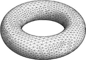
Figure 2. Triangulation of a torus

2.4. Sobolev, trace, and Stokes on a curved cylinder

This subsection includes basic analysis tools that will be used later in the proofs. The constants in the following estimates must be uniform in the geometry of the boundaries of our interest.

The first lemma contains the Sobolev embedding and the trace theorem. We remind the reader that their constants are uniform for all $\mathsf{C}\in\mathcal{C}^{(1)}$. These results are well-known so we omit the proof.

Lemma 1.

Let $\mathsf{C}_{1}\in\mathcal{C}^{(1)}$ be a curved cylinder with base $\mathsf{T}_{1}\in\mathcal{T}^{(1)}$. Let $\nabla u\in L^{p}(\mathsf{C}_{1})$ with either $\int_{\mathsf{C}_{1}}u\mathop{\kern 0.0pt\mathrm{d}}\!{}x=0$ or $u\bigr{\rvert}_{\mathsf{T}_{1}}=0$. and $p\in[1,3)$. Then there exists a constant $C_{p}$ depending only on $p$, such that

$$\left\lVert u\right\rVert_{L^{p^{\star}}(\mathsf{C}_{1})}\leq C_{p}\left\lVert\nabla u\right\rVert_{L^{p}(\mathsf{C}_{1})}.$$

Here $p^{\star}=\frac{dp}{d-p}$. Note that $C_{p}$ does not depend on $\mathsf{C}_{1}$. Moreover, with $p^{*}=\frac{(d-1)p}{d-p}$,

$$\left\lVert u\right\rVert_{L^{p^{*}}(\mathsf{T}_{1})}\leq C_{p}\left\lVert\nabla u\right\rVert_{L^{p}(\mathsf{C}_{1})}.$$

In this paper, $d=\dim\mathsf{C}_{1}=3$.

The next lemma is for the local boundary linear Stokes estimate, which is an extension of [VY21, Corollary 2.3]. The only difference is that the boundary part $\mathsf{T}_{2}$ is no longer flat, yet the bound is still uniform for all $\mathsf{C}_{1}\in\mathcal{C}^{(1)}$.

Lemma 2.

Let $\mathsf{C}_{1}\in\mathcal{C}^{(1)}$ be a curved cylinder with base $\mathsf{T}_{1}\in\mathcal{T}^{(1)}$. Let $\mathsf{C}_{2}$ be the image of a diffeomorphism $\psi$ associated with $\mathsf{C}_{1}$, and denote its base by $\mathsf{T}_{2}$. Let $1<p_{2}<p_{1}<\infty$, $1<q_{1},q_{2}<\infty$, $f\in L^{p_{1}}(-4,0;L^{q_{1}}(\mathsf{C}_{2}))$. If $(u,P)$ solves the linear evolutionary Stokes system

$$\begin{cases}\partial_{t}u+\nabla P=\Delta u+f&\text{ in }(-4,0)\times\mathsf{C}_{2}\\ \operatorname{div}u=0&\text{ in }(-4,0)\times\mathsf{C}_{2}\\ u=0&\text{ on }(-4,0)\times\mathsf{T}_{2}\;,\end{cases}$$

then there exists a decomposition $u=u_{1}+u_{2}$ such that for any $q^{\prime}<\infty$, there exists a constant $C=C(p_{1},p_{2},q_{1},q_{2},q^{\prime})$ such that

$$\left\lVert|\partial_{t}u_{1}|+|\nabla^{2}u_{1}|\right\rVert_{L^{p_{1}}(-1,0;L^{q_{1}}(\mathsf{C}_{1}))}+\left\lVert|\partial_{t}u_{2}|+|\nabla^{2}u_{2}|\right\rVert_{L^{p_{2}}(-1,0;L^{q^{\prime}}(\mathsf{C}_{1}))}$$

$$\qquad\leq C\left(\left\lVert f\right\rVert_{L^{p_{1}}(-4,0;L^{q_{1}}(\mathsf{C}_{2}))}+\left\lVert|u|+|\nabla u|+|P|\right\rVert_{L^{p_{2}}(-4,0;L^{q_{2}}(\mathsf{C}_{2}))}\right).$$

In particular, $C$ does not depend on the geometry of $\mathsf{C}_{1}$.

The proof of this lemma relies on Lemma 1, and also the corresponding uniform bound for boundary estimates and the Cauchy problem for the Stokes with curved boundary. See [MS97].

Proof.

Pick a set $\Omega$ with $C^{2}$ boundary such that $\mathsf{C}_{1}\subset\Omega\subset\mathsf{C}_{2}$. Note that the $C^{2}$ norm of $\partial\Omega$ can be uniformly bounded for all $\mathsf{C}_{1}\in\mathcal{C}^{(1)}$. By [Ser14, Theorem 4.5], there exists a unique solution $u_{1}$ to the initial-boundary value problem

$$\begin{cases}\partial_{t}u_{1}+\nabla P_{1}=\Delta u_{1}+f&\text{ in }(-4,0)\times\Omega\\ \operatorname{div}u_{1}=0&\text{ in }(-4,0)\times\Omega\\ u_{1}=0&\text{ on }(-4,0)\times\partial\Omega\\ u_{1}\bigr{\rvert}_{t=-4}=0&\text{ in }\Omega\end{cases}$$

with bound

$$\left\lVert|\partial_{t}u_{1}|+|\nabla P_{1}|\right\rVert_{L^{p_{1}}(-4,0;L^{q_{1}}(\Omega))} +\left\lVert u_{1}\right\rVert_{L^{p_{1}}(-4,0;W^{2,q_{1}}(\Omega))}$$

$$\qquad\leq C\left\lVert f\right\rVert_{L^{p_{1}}(-4,0;L^{q_{1}}(\Omega))},$$

where $C=C(p_{1},q_{1},\Omega)$. Dependence on $\Omega$ can be dropped if the $C^{2}$ norm of $\partial\Omega$ is uniformly bounded (see [MS95, MS97, Lemma 1.2]).

Let $u_{2}=u-u_{1}$, then $u_{2}$ is a solution to

$$\begin{cases}\partial_{t}u_{2}+\nabla P_{2}=\Delta u_{2}&\text{ in }(-4,0)\times\Omega\\ \operatorname{div}u_{2}=0&\text{ in }(-4,0)\times\Omega\\ u_{2}=0&\text{ on }(-4,0)\times(\partial\Omega\cap\mathsf{T}_{2})\quad.\end{cases}$$

The local boundary estimates of Stokes equation in [Ser14] imply the following bound:

$$\left\lVert|\partial_{t}u_{2}|+|\nabla^{2}u_{2}|\right\rVert_{L^{p_{2}}(-1,0;L^{q^{\prime}}(\mathsf{C}_{1}))}$$

$$\qquad\leq C\left\lVert|u_{2}|+|\nabla u_{2}|+|P_{2}|\right\rVert_{L^{p_{2}}(-4,0;L^{\min\left\{q_{1},q_{2}\right\}}(\Omega))},$$

where $C=C(p_{2},q_{1},q_{2},\Omega)$. Again, the dependence on $\Omega$ can be dropped. Combining with estimates of $u_{1}$, we finish the proof of the lemma. ∎

Finally, we quote the following global Stokes theorem in [Sol02, Theorem 1.1].

Lemma 3.

Let $\Omega\subset\mathbb{R}^{d}$ be a bounded $C^{2}$ domain with $d\geq 2$, and $T>0$. Let $f\in L^{p}(0,T;L^{q}(\Omega))$ and $u_{0}\in B^{2-2/p}_{q,p}(\Omega)$, where $B_{q,p}^{l}(\Omega)$ is the Besov space, and $1<p,q<\infty$ satisfy $2-2/p<1/q$. Then the following linear evolutionary Stokes system

$$\begin{cases}\partial_{t}u+\nabla P=\Delta u+f&\text{ in }(0,T)\times\Omega\\ \operatorname{div}u=0&\text{ in }(0,T)\times\Omega\\ u=0&\text{ on }(0,T)\times\partial\Omega\\ u\bigr{\rvert}_{t=0}=u_{0}&\text{ in }\Omega\end{cases}$$

has a unique solution $u\in L^{p}(0,T;W^{2,q}(\Omega))$ with $\nabla P,\partial_{t}u\in L^{p}(0,T;L^{q}(\Omega))$, and

$$\left\lVert u\right\rVert_{L^{p}(0,T;W^{2,q}(\Omega))}+\left\lVert\partial_{t}u\right\rVert_{L^{p}(0,T;L^{q}(\Omega))}+\left\lVert\nabla p\right\rVert_{L^{p}(0,T;L^{q}(\Omega))}$$

$$\qquad\leq C\left(\left\lVert f\right\rVert_{L^{p}(0,T;L^{q}(\Omega))}+\left\lVert u_{0}\right\rVert_{B^{2-2/p}_{q,p}(\Omega)}\right),$$

where $C=C(\Omega,p,q)$.

3. Boundary vorticity estimate

In this section, we provide several estimates for the boundary vorticity $\omega^{\nu}=\operatorname{curl}u^{\nu}$. We first use linear parabolic theory to directly derive a coarse estimate. This estimate will degenerate in the inviscid limit. We compensate with a refined estimate Theorem 3, which is based on a new local boundary vorticity estimate for the linear Stokes system.

3.1. Naïve linear global estimate

By treating Navier–Stokes equation as a Stokes system with a forcing term, we can derive the following naïve bound using parabolic regularization.

Proposition 1.

Let $u^{\nu}\in C_{\mathrm{w}}(0,T;L^{2}(\Omega))\cap L^{2}(0,T;H^{1}_{0}(\Omega))$ be a weak solution to ($\mathrm{NSE}_{\nu}$) with divergence-free initial value $u^{\nu}(0)\in H^{1}_{0}(\Omega)$ and force $f^{\nu}\in L^{\frac{4}{3}}(0,T;L^{\frac{6}{5}}(\Omega))$. There exists a universal constant $C(\Omega)$, independent of $u^{\nu}$ and $\nu$, such that

$$\int_{(0,T)\times\partial\Omega}|\nu\nabla u^{\nu}|^{\frac{4}{3}}\mathop{\kern 0.0pt\mathrm{d}}\!{}x^{\prime}\mathop{\kern 0.0pt\mathrm{d}}\!{}t\leq C(\Omega)\Biggl{[}\left\lVert f^{\nu}\right\rVert_{L^{\frac{4}{3}}(0,T;L^{\frac{6}{5}}(\Omega))}^{\frac{4}{3}}+$$

$$\qquad+\left\lVert u^{\nu}\right\rVert_{L^{\infty}(0,T;L^{2}(\Omega))}^{\frac{2}{3}}\left(\int_{(0,T)\times\Omega}|\nabla u^{\nu}|^{2}\mathop{\kern 0.0pt\mathrm{d}}\!{}x\mathop{\kern 0.0pt\mathrm{d}}\!{}t+\nu^{\frac{1}{3}}\left\lVert u^{\nu}(0)\right\rVert_{H^{1}(\Omega)}^{\frac{2}{3}}\right)\Biggr{]}.$$

Proof.

Let $u^{\nu}(t,x)=\nu v(\nu t,x)$ and $f^{\nu}(t,x)=\nu^{2}g(\nu t,x)$, then $v$ solves ($\mathrm{NSE}_{1}$) in $(0,\nu T)\times\Omega$ with unit viscosity and force $g$. Treating the nonlinear term $v\cdot\nabla v$ as a force, then Lemma 3 implies

$$\left\lVert v\right\rVert_{L^{\frac{4}{3}}(0,\nu T;W^{2,\frac{6}{5}}(\Omega))} \leq C(\Omega)\left(\left\lVert-v\cdot\nabla v+g\right\rVert_{L^{\frac{4}{3}}(0,\nu T;L^{\frac{6}{5}}(\Omega))}+\left\lVert v_{0}\right\rVert_{B^{\frac{1}{2}}_{\frac{6}{5},\frac{4}{3}}(\Omega)}\right).$$

Here $C(\Omega)$ represent general constants depending only on $\Omega$, and $v_{0}=v\bigr{\rvert}_{t=0}$. For the forcing term,

$$\left\lVert v\cdot\nabla v\right\rVert_{L^{\frac{4}{3}}(0,\nu T;L^{\frac{6}{5}}(\Omega))} \leq\left\lVert v\right\rVert_{L^{4}(0,\nu T,L^{3}(\Omega))}\left\lVert\nabla v\right\rVert_{L^{2}((0,\nu T)\times\Omega)}$$

$$\leq\left\lVert v\right\rVert_{L^{\infty}(0,\nu T;L^{2}(\Omega))}^{\frac{1}{2}}\left\lVert v\right\rVert_{L^{2}(0,\nu T;L^{6}(\Omega))}^{\frac{1}{2}}\left\lVert\nabla v\right\rVert_{L^{2}((0,\nu T)\times\Omega)}$$

$$\leq C(\Omega)\left\lVert v\right\rVert_{L^{\infty}(0,\nu T;L^{2}(\Omega))}^{\frac{1}{2}}\left\lVert\nabla v\right\rVert_{L^{2}((0,\nu T)\times\Omega)}^{\frac{3}{2}},$$

where in the last step we used Sobolev embedding in $\Omega\subset\mathbb{R}^{3}$. For the initial value, we use Besov embedding and interpolation so

$$\left\lVert v_{0}\right\rVert_{B^{\frac{1}{2}}_{\frac{6}{5},\frac{4}{3}}(\Omega)}\leq C(\Omega)\left\lVert v_{0}\right\rVert_{B^{\frac{1}{2}}_{\frac{4}{3},\frac{4}{3}}(\Omega)} \leq C(\Omega)\left\lVert v_{0}\right\rVert_{H^{\frac{1}{2}}(\Omega)}$$

$$\leq C(\Omega)\left\lVert v_{0}\right\rVert_{L^{2}(\Omega)}^{\frac{1}{2}}\left\lVert v_{0}\right\rVert_{H^{1}(\Omega)}^{\frac{1}{2}}.$$

By the Sobolev embedding and the trace theorem in $\Omega$,

$$\left\lVert\nabla v\right\rVert_{L^{\frac{4}{3}}((0,\nu T)\times\partial\Omega)} \leq C(\Omega)\left\lVert\nabla v\right\rVert_{L^{\frac{4}{3}}(0,\nu T;W^{\frac{1}{6},\frac{6}{5}}(\partial\Omega))}$$

$$\leq C(\Omega)\left\lVert\nabla v\right\rVert_{L^{\frac{4}{3}}(0,\nu T;W^{1,\frac{6}{5}}(\Omega))}$$

$$\leq C(\Omega)\left\lVert v\right\rVert_{L^{\frac{4}{3}}(0,\nu T;W^{2,\frac{6}{5}}(\Omega))}.$$

Combine the above estimates, we have

$$\left\lVert\nabla v\right\rVert_{L^{\frac{4}{3}}((0,\nu T)\times\partial\Omega)} \lesssim\left\lVert v\right\rVert_{L^{\infty}(0,\nu T;L^{2}(\Omega))}^{\frac{1}{2}}\left(\left\lVert\nabla v\right\rVert_{L^{2}((0,\nu T)\times\Omega)}^{\frac{3}{2}}+\left\lVert v_{0}\right\rVert_{H^{1}(\Omega)}^{\frac{1}{2}}\right)$$

$$\qquad+\left\lVert g\right\rVert_{L^{\frac{4}{3}}(0,\nu T;L^{\frac{6}{5}}(\Omega))}.$$

Note the scaling of the $v$ and $g$, we have for any $p\in[1,\infty]$ and any norm $X$

$$\left\lVert u^{\nu}\right\rVert_{L^{p}(0,T;X)} =\nu^{1-\frac{1}{p}}\left\lVert v\right\rVert_{L^{p}(0,\nu T;X)}, \left\lVert f^{\nu}\right\rVert_{L^{p}(0,T;X)} =\nu^{2-\frac{1}{p}}\left\lVert g\right\rVert_{L^{p}(0,\nu T;X)}.$$

By this scaling, we have the corresponding estimates on $u^{\nu}$ as

$$\nu^{-\frac{1}{4}}\left\lVert\nabla u^{\nu}\right\rVert_{L^{\frac{4}{3}}((0,T)\times\partial\Omega)}\lesssim\nu^{-\frac{5}{4}}\left\lVert f^{\nu}\right\rVert_{L^{\frac{4}{3}}(0,T;L^{\frac{6}{5}}(\Omega))}+$$

$$\qquad+\nu^{-\frac{1}{2}}\left\lVert u^{\nu}\right\rVert_{L^{\infty}(0,T;L^{2}(\Omega))}^{\frac{1}{2}}\left(\nu^{-\frac{3}{4}}\left\lVert\nabla u^{\nu}\right\rVert_{L^{2}((0,T)\times\Omega)}^{\frac{3}{2}}+\nu^{-\frac{1}{2}}\left\lVert u^{\nu}(0)\right\rVert_{H^{1}(\Omega)}^{\frac{1}{2}}\right).$$

This completes the proof of the proposition. ∎

In the inviscid limit $\nu\to 0$, the main term $\int_{(0,T)\times\Omega}|\nabla u^{\nu}|^{2}\mathop{\kern 0.0pt\mathrm{d}}\!{}x\mathop{\kern 0.0pt\mathrm{d}}\!{}t$ cannot be uniformly bounded, and the force $\left\lVert f^{\nu}\right\rVert_{L^{\frac{4}{3}}(0,T;L^{\frac{6}{5}}(\Omega))}$ does not vanish. Therefore, we need to look for another bound that does not degenerate in the inviscid limit.

3.2. Local estimate for the linear Stokes system

To overcome the degeneracy of the naïve bound in the inviscid limit, we show an improved bound in the next subsection, which is based on the following linear estimates for the Stokes system at the unit scale and unit viscosity.

Proposition 2.

Let $\mathsf{C}_{2}\in\mathcal{C}^{(2)}$ with base $\mathsf{T}_{2}$, and denote $\mathsf{Q}_{2}=(-4,0)\times\mathsf{C}_{2}$, $\bar{\mathsf{Q}}_{2}=(-4,0)\times\mathsf{T}_{2}$. Suppose $u\in L^{2}(-4,0;H^{1}(\mathsf{C}_{2}))$ is a solution to the following Stokes system with forcing term $f\in L^{1}(-4,0;L^{\frac{6}{5}}(\mathsf{C}_{2}))$:

(6) $$\begin{cases}\partial_{t}u+\nabla P=\Delta u+f&\text{ in }\mathsf{Q}_{2}\\ \operatorname{div}u=0&\text{ in }\mathsf{Q}_{2}\\ u=0&\text{ on }\bar{\mathsf{Q}}_{2}\;.\end{cases}$$

Then the average vorticity on the boundary is bounded by

$$\left\lvert\int_{\bar{\mathsf{Q}}_{1}}\omega(t,x^{\prime},0)\mathop{\kern 0.0pt\mathrm{d}}\!{}x^{\prime}\mathop{\kern 0.0pt\mathrm{d}}\!{}t\right\rvert \leq\int_{\mathsf{T}_{1}}\left\lvert\int_{-1}^{0}\omega(t,x^{\prime},0)\mathop{\kern 0.0pt\mathrm{d}}\!{}t\right\rvert\mathop{\kern 0.0pt\mathrm{d}}\!{}x^{\prime}$$

$$\leq C\left(\left\lVert\nabla u\right\rVert_{L_{t}^{2}L_{x}^{2}(\mathsf{Q}_{2})}+\left\lVert f\right\rVert_{L_{t}^{1}L_{x}^{6/5}(\mathsf{Q}_{2})}\right).$$

Proof.

The proof is the same as the one in [VY21], with only some mild modifications to resolve the curved boundary issue. Without loss of generality, assume by linearity that $\left\lVert\nabla u\right\rVert_{L_{t}^{2}L_{x}^{2}(\mathsf{Q}_{2})},\left\lVert f\right\rVert_{L_{t}^{1}L_{x}^{6/5}(\mathsf{Q}_{2})}\leq 1$.

For $t\in(-3,0)$, $x\in\mathsf{C}_{2}$, we define

$$U(t,x)=\int_{t-1}^{t}u(s,x)\mathop{\kern 0.0pt\mathrm{d}}\!{}s.$$

Denote $\rho(t)=\mathbf{1}_{[0,1]}(t)$, then $U=u*_{t}\rho$, where $*_{t}$ stands for convolution in $t$ variable only. If we denote $Q=P*_{t}\rho$, and $F=f*_{t}\rho$, then $U$ satisfies the Stokes system:

$$\begin{cases}\partial_{t}U+\nabla Q=\Delta U+F&\text{ in }(-3,0)\times\mathsf{C}_{2}\\ \operatorname{div}U=0&\text{ in }(-3,0)\times\mathsf{C}_{2}\\ U=0&\text{ on }(-3,0)\times\mathsf{T}_{2}\;.\end{cases}$$

We have via Sobolev embedding Lemma 1 and $u\bigr{\rvert}_{\mathsf{T}_{2}}=0$ that

(7) $$\left\lVert u\right\rVert_{L_{t}^{2}L_{x}^{6}\left(\mathsf{Q}_{2}\right)}\leq C.$$

Since $\partial_{t}U(t,x)=u(t,x)-u(t-1,x)$, we have

$$\left\lVert\partial_{t}U\right\rVert_{L_{t}^{2}L_{x}^{6}((-3,0)\times\mathsf{C}_{2})}\leq C.$$

On the other hand, the Laplacian of $U$ is bounded by

$$\left\lVert\Delta U\right\rVert_{L_{t}^{\infty}H_{x}^{-1}((-3,0)\times\mathsf{C}_{2})}\leq C\left\lVert\Delta u\right\rVert_{L_{t}^{2}H_{x}^{-1}(\mathsf{Q}_{2})}\leq C\left\lVert\nabla u\right\rVert_{L^{2}(\mathsf{Q}_{2})}\leq C.$$

Note that the Sobolev constants depend on the geometry of $\mathsf{C}_{2}$. However, they are uniformly bounded as long as $\mathsf{C}_{2}\in\mathcal{C}^{(2)}$, since the Lipschitz norms of the boundary are uniformly bounded. Again by convolution, we bound $F$ by

$$\left\lVert F\right\rVert_{L_{t}^{\infty}H^{-1}_{x}((-3,0)\times\mathsf{C}_{2})}\leq C\left\lVert F\right\rVert_{L_{t}^{\infty}L_{x}^{\frac{6}{5}}((-3,0)\times\mathsf{C}_{2})}\leq C.$$

Next, we estimate $Q$. Using $\nabla Q=\Delta U+F-\partial_{t}U$ we have

$$\left\lVert\nabla Q\right\rVert_{L_{t}^{2}H_{x}^{-1}((-3,0)\times\mathsf{C}_{2})}\leq C.$$

Without loss of generality, we assume that the average of $Q$ is zero at every $t$. Then by Nečas theorem (see [Ser14], Section 1.4),

$$\left\lVert Q\right\rVert_{L^{2}_{t,x}((-3,0)\times\mathsf{T}_{2})}\leq C.$$

Note that the constant of Nečas theorem also depends on the Lipschitz norm of $\partial\mathsf{C}_{1}$, which is uniform for all $\mathsf{C}_{1}\in\mathcal{C}^{(1)}$.

By Lemma 2, we can split $U=U_{1}+U_{2}$, where for any $p<\infty$, we have

$$\left\lVert\left\lvert\partial_{t}U_{1}\right\rvert+\left\lvert\nabla^{2}U_{1}\right\rvert\right\rVert_{L_{t}^{p}L_{x}^{\frac{6}{5}}(\mathsf{Q}_{1})}+\left\lVert\left\lvert\partial_{t}U_{2}\right\rvert+\left\lvert\nabla^{2}U_{2}\right\rvert\right\rVert_{L_{t}^{2}L_{x}^{p}(\mathsf{Q}_{1})}\leq C.$$

Denote $\Omega(t,z):=\int_{\mathsf{T}_{1}}\left\lvert\nabla U(t,x^{\prime}-zn(x^{\prime}))\right\rvert\mathop{\kern 0.0pt\mathrm{d}}\!{}x^{\prime}$, then $\partial_{z}\Omega$ is bounded in

$$\partial_{z}\Omega\in L_{t}^{2}L_{z}^{p}+L_{t}^{p}L_{z}^{\frac{6}{5}}((-1,0)\times(0,1)).$$

for any $p<\infty$. Note that

$$\partial_{t}\Omega=\int_{\mathsf{T}_{1}}\left\lvert\nabla u\right\rvert\mathop{\kern 0.0pt\mathrm{d}}\!{}x^{\prime}\in L^{2}_{t,z}((-1,0)\times(0,1)).$$

Since by interpolation, $L_{t}^{1}L_{z}^{\infty}\cap L_{t}^{\infty}L_{z}^{1}\subset L^{2}_{t,z}$, by duality $\partial_{t}\Omega$ is bounded in $L^{2}_{t,z}\subset L_{t}^{1}L_{z}^{\infty}+L_{t}^{\infty}L_{z}^{1}$. Similarly, $\partial_{z}\Omega$ is bounded in

$$\partial_{z}\Omega\in L_{t}^{2}L_{z}^{p}+L_{t}^{p}L_{z}^{\frac{6}{5}}((-1,0)\times(0,1))\subset L_{t}^{r}L_{z}^{\infty}+L_{t}^{\infty}L_{z}^{r}((-1,0)\times(0,1))$$

for some $p>6$ with $r>1$ sufficiently small. Now we can use [VY21, Lemma 2.4] to show $\Omega$ is continuous up to the boundary with oscillation bounded by

$$\left\lVert\Omega\right\rVert_{\mathrm{osc}((-1,0)\times(0,1))}\leq C.$$

Since the average of $\Omega$ is also bounded as

$$\int\Omega\mathop{\kern 0.0pt\mathrm{d}}\!{}{x_{d}}\mathop{\kern 0.0pt\mathrm{d}}\!{}t=\int_{\mathsf{Q}_{1}}\left\lvert\nabla u\right\rvert\mathop{\kern 0.0pt\mathrm{d}}\!{}x\mathop{\kern 0.0pt\mathrm{d}}\!{}t\leq C,$$

we have $\Omega$ is bounded in $L^{\infty}$, in particular

$$\int_{\mathsf{T}_{1}}\left\lvert\int_{-1}^{0}\nabla u(t,x^{\prime},0)\mathop{\kern 0.0pt\mathrm{d}}\!{}t\right\rvert\mathop{\kern 0.0pt\mathrm{d}}\!{}x^{\prime}=\Omega(0,0)\leq C.$$

This concludes the proof of this proposition. ∎

3.3. Refined global estimate

Now we are ready to prove the main boundary vorticity estimate.

Proof of Theorem 3.

The proof can be divided into four steps. In the first step, we triangularize $\partial\Omega$ and obtain a course partition $(0,T)\times\partial\Omega$. Next, we construct $\sigma$-algebra $\mathcal{F}$, which is generated by a finer partition of $(0,T)\times\partial\Omega$, by introducing a suitability criterion. Then we verify that in each piece of the partition, average boundary vorticity is controlled by the maximal function of the energy dissipation and the external force. Finally, we estimate the $L^{\frac{4}{3}}$ weak norm of the averaged vorticity function.

Up to rescaling $u^{\nu}(t,x)=\nu u(\nu t,x)$ and $f^{\nu}=\nu^{2}f(\nu t,x)$, we assume $\nu=1$ first and drop the superscript for simplicity.

Step 1

First, we introduce an initial partition of $(0,T)\times\Omega$ as the following. Select $L_{0}=4^{-K}T$, where $K=\left(\left\lceil\log_{4}\left(\frac{T}{\delta^{2}}\right)\right\rceil\right)_{+}$ is the smallest nonnegative integer such that $L_{0}=4^{-K}T\leq\delta^{2}$. Set $r_{0}=\frac{1}{2}\sqrt{L_{0}}=2^{-K-1}\sqrt{T}\leq\delta$, then

$$r_{0}\leq\frac{1}{2}\min\left\{\delta,\sqrt{T}\right\}<2r_{0}.$$

Let $\{\mathsf{T}_{r_{0}}^{(i)}\}_{i}\subset\mathcal{T}^{(r_{0})}$ be a partition of $\partial\Omega$ with size $r_{0}$, as specified in Assumption 1. Then

$$(0,T)\times\partial\Omega\simeq\bigsqcup_{j=1}^{4^{K}}\bigsqcup_{i}\bar{\mathsf{Q}}^{(i,j)}\quad\text{ where }\bar{\mathsf{Q}}^{(i,j)}=((j-1)L_{0},jL_{0})\times\mathsf{T}_{r_{0}}^{(i)}.$$

We denote $\bar{\mathcal{Q}}_{0}=\left\{\bar{\mathsf{Q}}^{(i,j)}\right\}_{i,j}$. By part (v) of Section 2.2, each $\bar{\mathsf{Q}}^{(i,j)}$ admits a sequence of dyadic decomposition. For $k\geq 1$, denote $\bar{\mathcal{Q}}_{k}$ to be the set of dyadic decompositions of spacetime curved triangles in $\bar{\mathcal{Q}}_{k-1}$. Then any $\bar{\mathsf{Q}}\in\bar{\mathcal{Q}}_{k}$ is a Cartesian product of curved triangle of size $r_{k}:=2^{-k}r_{0}$ in space and length $r_{k}^{2}=4^{-k}r_{0}^{2}$ in time.

Step 2

The next goal is to find a partition of $(0,T)\times\Omega$ consisting of “suitable” cubes, defined as follows. Let $\bar{\mathsf{Q}}=(\hat{t}-r_{k}^{2},\hat{t})\times\mathsf{T}_{r_{k}}\in\bar{\mathcal{Q}}_{k}$ for some $\hat{t}\in(0,T]$ and $\mathsf{T}_{r_{k}}\in\mathcal{T}^{(r_{k})}$. Denote $\hat{x}$ to be the barycenter of $\mathsf{T}_{r_{k}}$. We say $\bar{\mathsf{Q}}$ is suitable if both $\hat{t}\geq 4r_{k}^{2}$ and

(S) $$\fint\limits_{\hat{t}-4r_{k}^{2}}^{\hat{t}}\;\fint\limits_{\partial\Omega\cap B_{2r_{k}}(\hat{x})}\fint\limits_{0}^{2r_{k}}\left(|\nabla u|^{2}+|f|^{\frac{4}{3}}\right)(t,x^{\prime}-zn(x^{\prime}))\mathop{\kern 0.0pt\mathrm{d}}\!{}z\mathop{\kern 0.0pt\mathrm{d}}\!{}x^{\prime}\mathop{\kern 0.0pt\mathrm{d}}\!{}t\leq c_{0}r_{k}^{-4}.$$

for some $c_{0}$ to be determined. Recall $n(x^{\prime})$ is the outer normal vector at $x^{\prime}\in\partial\Omega$.

Now we construct a partition according to suitability. Denote $\mathcal{S}_{0}\subset\bar{\mathcal{Q}}_{0}$ to be the set of suitable cubes, $\mathcal{N}_{0}=\bar{\mathcal{Q}}_{0}\setminus\mathcal{S}_{0}$ be the set of non-suitable cubes. For $k\geq 1$, we perform a dyadic decomposition on each cube $\bar{\mathsf{Q}}\in\mathcal{N}_{k-1}$, then put the suitable ones in $\mathcal{S}_{k}$ and non-suitable ones in $\mathcal{N}_{k}$. This process may continue indefinitely, and we define $\mathcal{S}=\cup_{k}\mathcal{S}_{k}$ to be the set of suitable cubes that we obtained from this process.

We claim that $\mathcal{S}$ is a partition of $(0,T)\times\partial\Omega$. It is easy to see from our process that cubes in $\mathcal{S}$ are mutually disjoint. Moreover, for almost every $(t,x^{\prime})\in(0,T)\times\partial\Omega$, the cube whose closure contains $(t,x^{\prime})$ becomes suitable if the cube is sufficiently small, by a partial regularity argument. Indeed, denote the singular set $\operatorname{Sing}(u,f)$ to be the complement of the closure of ${\bigcup_{\bar{\mathsf{Q}}\in\mathcal{S}}\bar{\mathsf{Q}}}$ in $(0,T)\times\partial\Omega$. For every $(\hat{t},\hat{x}^{\prime})\in\operatorname{Sing}(u,f)$, for every $k>0$, there exists a cube $\bar{\mathsf{Q}}_{k}\in\mathcal{N}_{k}$ such that $\bar{\mathsf{Q}}_{k}$ fails the suitability codition (S). Then we find a neighborhood of $(\hat{t},\hat{x}^{\prime})$ in $(0,T)\times\Omega$ which is

$$U=\left\{(t,x^{\prime}-zn(x^{\prime})):t\in(\hat{t}-4r_{k}^{2},\hat{t}),x^{\prime}\in\partial\Omega\cap B_{2r_{k}}(\hat{x}),z\in(0,2r_{k})\right\},$$

such that $\int_{U}|\nabla u|^{2}+|f|^{\frac{4}{3}}\mathop{\kern 0.0pt\mathrm{d}}\!{}x\mathop{\kern 0.0pt\mathrm{d}}\!{}t\gtrsim r_{k}$. Moreover, this neighborhood is comparable with a parabolic cylinder of radius $r_{k}$. These neighborhoods form an open cover of $\operatorname{Sing}(u,f)$. By the covering lemma, we find a disjoint subcollection $U_{i}$ which covers $\operatorname{Sing}(u,f)$ if dilating by a factor of 5. The radii are summable because $\sum_{i}r_{k}\lesssim\sum_{i}\int_{U_{i}}|\nabla u|^{2}+|f|^{\frac{4}{3}}\mathop{\kern 0.0pt\mathrm{d}}\!{}x\mathop{\kern 0.0pt\mathrm{d}}\!{}t<\infty$, so the parabolic Hausdorff dimension of $\operatorname{Sing}(u,f)$ is at most 1.

Define $\mathcal{F}=\sigma(\mathcal{S})$ to be the $\sigma$-algebra generated by these countably many suitable cubes. Then the conditional expectation $\tilde{\omega}:=\mathbb{E}[\omega|\mathcal{F}]$ is simply a piecewise function, taking the average value of $\omega$ on each $\bar{\mathsf{Q}}\in\mathcal{S}$.

Next we prove claim (i) and (ii). First, we show the set $A=(0,4^{-l-1})\times\partial\Omega$ is $\mathcal{F}$-measurable. If $4^{-l}T\leq\delta^{2}$ and $l\geq 0$, then $4^{-l-1}T\leq\frac{1}{4}\min\left\{\delta^{2},T\right\}<4r_{0}^{2}$. Hence $4^{-l-1}T=4^{-l-1}\cdot 4^{K+1}r_{0}^{2}=4^{-(l+1-K)}\cdot 4r_{0}^{2}=4r_{k^{\prime}}^{2}$ for some $k^{\prime}>0$, and $A=(0,4r_{k^{\prime}}^{2})\times\partial\Omega$. On the one hand, for $k<k^{\prime}$, $\mathcal{S}_{k}$ only contains cubes of the form $(\hat{t}-r_{k}^{2},\hat{t})\times\mathsf{T}_{r_{k}}$ with $\hat{t}-r_{k}^{2}\geq 3r_{k}^{2}>4r_{k^{\prime}}^{2}$, so $A$ is disjoint from every cube in $\mathcal{S}_{k}$. On the other hand, for $k\geq k^{\prime}$, $\mathcal{S}_{k}\subset\bar{\mathcal{Q}}_{k}$ only contains cubes of the form $(jr_{k}^{2},(j+1)r_{k}^{2})\times\mathsf{T}_{r_{k}}$. Since $4r_{k^{\prime}}^{2}=4^{k-k^{\prime}+1}r_{k}^{2}$, each cube in $\mathcal{S}_{k}$ is either contained in $A$ or disjoint from $A$. In conclusion, every set in $\mathcal{S}$ is either a subset of $A$ or a subset of $(0,T)\times\partial\Omega\setminus A$, hence $A\in\sigma(\mathcal{S})=\mathcal{F}$.

To prove (ii), note that each $\bar{\mathsf{Q}}$ in $\mathcal{S}$ has size at most $r_{0}<\delta$ in space and $r_{0}^{2}<\delta^{2}$ in time, so for $(t_{1},x_{1}),(t_{2},x_{2})\in\bar{\mathsf{Q}}$,

$$|\varphi(t_{1},x_{1})-\varphi(t_{2},x_{2})| \leq|\varphi(t_{1},x_{1})-\varphi(t_{2},x_{1})|+|\varphi(t_{2},x_{1})-\varphi(t_{2},x_{2})|$$

$$\leq\left\lVert\partial_{t}\varphi\right\rVert_{L^{\infty}}|t_{1}-t_{2}|+\left\lVert\nabla\varphi\right\rVert_{L^{\infty}}|x_{1}-x_{2}|$$

$$\leq\delta^{2}\left\lVert\partial_{t}\varphi\right\rVert_{L^{\infty}}+\delta\left\lVert\nabla\varphi\right\rVert_{L^{\infty}}.$$

Step 3

Take any cube $\bar{\mathsf{Q}}\in\mathcal{S}_{k}$. By using the canonical scaling of the Navier-Stokes equation $u_{r}(t,x):=ru(r^{2}t+\hat{t},rx)$ and $f_{r}(t,x):=r^{3}f(r^{2}t+\hat{t},rx)$ with size $r=r_{k}$, $u_{r}$ solves the Stokes equation (6) in $(-4,0)\times\mathsf{C}_{2}$ with some $\mathsf{C}_{2}\in\mathcal{C}^{(2)}$ and force term $f_{r}-u_{r}\cdot\nabla u_{r}$, and (S) implies

$$\left\lVert\nabla u_{r}\right\rVert_{L^{2}((-4,0)\times\mathsf{C}_{2})} \leq c_{0}^{\frac{1}{2}},$$

$$\left\lVert f_{r}\right\rVert_{L^{1}(-4,0;L^{\frac{6}{5}}(\mathsf{C}_{2}))} \leq\left\lVert f_{r}\right\rVert_{L^{\frac{4}{3}}((-4,0)\times\mathsf{C}_{2})}\lesssim c_{0}^{\frac{3}{4}},$$

$$\left\lVert u_{r}\cdot\nabla u_{r}\right\rVert_{L^{1}(-4,0;L^{\frac{6}{5}}(\mathsf{C}_{2}))} \lesssim\left\lVert\nabla u_{r}\right\rVert_{L^{2}((-4,0)\times\mathsf{C}_{2})}\left\lVert u_{r}\right\rVert_{L^{2}(-4,0;L^{6}(\mathsf{C}_{2}))}\lesssim c_{0}.$$

In the last step we used the Sobolev embedding

$$\left\lVert u_{r}\right\rVert_{L^{2}(-4,0;L^{6}(\mathsf{C}_{2}))}\lesssim\left\lVert\nabla u_{r}\right\rVert_{L^{2}((-4,0)\times\mathsf{C}_{2})},$$

when $u_{r}=0$ on the base $\mathsf{T}_{2}$. Therefore, Proposition 2 implies that after scaling, the average vorticity is bounded by

$$|\tilde{\omega}|_{\bar{\mathsf{Q}}}:=\left\lvert\fint_{\bar{\mathsf{Q}}}\omega(t,x^{\prime})\mathop{\kern 0.0pt\mathrm{d}}\!{}x^{\prime}\mathop{\kern 0.0pt\mathrm{d}}\!{}t\right\rvert\leq\frac{1}{16}\gamma r_{k}^{-2},$$

where we choose $c_{0}=\frac{1}{C}\gamma^{2}\leq 1$.

Next, we separate two scenarios, $k=0$ and $k>0$. If $k=0$, then for any $\bar{\mathsf{Q}}\in\mathcal{S}_{0}$, for any $0<t<T$,

$$|\tilde{\omega}|_{\bar{\mathsf{Q}}}\leq\frac{1}{16}\gamma r_{0}^{-2}<\gamma\max\left\{\delta^{-2},T^{-1}\right\}.$$

If $k>0$, then $\bar{\mathsf{Q}}\in\mathcal{S}_{k}$ has an antecedent cube $\bar{\mathsf{P}}\in\mathcal{N}_{k-1}$. Cube $\bar{\mathsf{P}}=(\hat{t}-r_{k-1}^{2},\hat{t})\times\mathsf{T}_{r_{k-1}}$ is not suitable, so either of the following two cases must be true.

1. $\hat{t}<4r_{k-1}^{2}$. In this case, for any $(t,x)\in\bar{\mathsf{Q}}\subset\bar{\mathsf{P}}$,

   $$|\tilde{\omega}|_{\bar{\mathsf{Q}}}\leq\frac{1}{16}\gamma r_{k}^{-2}=\frac{1}{4}\gamma r_{k-1}^{-2}\leq\gamma\hat{t}^{-1}\leq\frac{\gamma}{t}.$$

2. $\hat{t}\geq 4r_{k-1}^{2}$, but

   $$\fint\limits_{\hat{t}-4r_{k-1}^{2}}^{\hat{t}}\;\fint\limits_{\partial\Omega\cap B_{2r_{k-1}}(\hat{x})}\fint\limits_{0}^{2r_{k-1}}\left(|\nabla u|^{2}+|f|^{\frac{4}{3}}\right)(t,x^{\prime}-zn(x^{\prime}))\mathop{\kern 0.0pt\mathrm{d}}\!{}z\mathop{\kern 0.0pt\mathrm{d}}\!{}x^{\prime}\mathop{\kern 0.0pt\mathrm{d}}\!{}t>c_{0}r_{k-1}^{-4}.$$

In the latter case, note that the integral region is comparable to $\mathsf{Q}$, the extension of $\bar{\mathsf{Q}}$, which is contained in $(0,T)\times\mathcal{U}_{\delta}(\partial\Omega,\Omega)$. We then know that for any $(t,x)\in\mathsf{Q}$, the parabolic maximal function is bounded from below by

$$M(t,x) :=\mathcal{M}((|\nabla u|^{2}+|f|^{\frac{4}{3}})\mathbf{1}_{[0,T]\times\mathcal{U}_{\delta}(\partial\Omega,\Omega)})(t,x)$$

$$:=\sup_{r>0}\fint_{t-r^{2}}^{t+r^{2}}\fint_{B_{r}(x)}\left(|\nabla u|^{2}+|f|^{\frac{4}{3}}\right)(s,y)\mathbf{1}_{[0,T]\times\mathcal{U}_{\delta}(\partial\Omega,\Omega)}(s,y)\mathop{\kern 0.0pt\mathrm{d}}\!{}y\mathop{\kern 0.0pt\mathrm{d}}\!{}s$$

$$\geq\frac{1}{C}c_{0}r_{k}^{-4}=\frac{\gamma^{2}}{C}r_{k}^{-4}.$$

Note that the parabolic maximal function $\mathcal{M}$ is a bounded map from $L^{1}(\mathbb{R}\times\mathbb{R}^{3})$ to $L^{1,\infty}(\mathbb{R}\times\mathbb{R}^{3})$.

In summary, for any $\bar{\mathsf{Q}}\in\mathcal{S}_{k}$, we have $|\tilde{\omega}|_{\bar{\mathsf{Q}}}\leq\frac{1}{16}\gamma r_{k}^{-2}\leq\gamma r_{k}^{-2}$, and

$$\text{ either }|\tilde{\omega}|_{\bar{\mathsf{Q}}}\leq\gamma\max\left\{\frac{1}{t},\frac{1}{\delta^{2}}\right\}\qquad\text{ or }M\bigr{\rvert}_{\mathsf{Q}}\geq\frac{\gamma^{2}}{C}r_{k}^{-4}.$$

Step 4

Denote $\mathcal{S}=\left\{\bar{\mathsf{Q}}^{(i)}\right\}$ and let $\bar{\mathsf{Q}}^{(i)}$ has size $r^{(i)}$. For any $r_{\star}=2^{l}r_{0}$ with $l\in\mathbb{Z}$, we have

$$\left\{(t,x^{\prime})\in(0,T)\times\partial\Omega:|\tilde{\omega}|>\gamma\max\left\{r_{\star}^{-2},t^{-1},\delta^{-2}\right\}\right\}$$

$$\subset\bigcup_{i}\left\{\bar{\mathsf{Q}}^{(i)}:r^{(i)}<r_{\star},M\bigr{\rvert}_{\mathsf{Q}^{(i)}}\geq\frac{\gamma^{2}}{C}(r^{(i)})^{-4}\right\}$$

$$\subset\bigcup_{i}\bigcup_{k=1}^{\infty}\left\{\bar{\mathsf{Q}}^{(i)}:r^{(i)}=2^{-k}r_{\star},M\bigr{\rvert}_{\mathsf{Q}^{(i)}}\geq\frac{\gamma^{2}}{C}(2^{-k}r_{\star})^{-4}\right\}.$$

Therefore the measure of the upper level set is controlled by the total measure of these suitable cubes, that is

$$\left\lvert\left\{\left\lvert\tilde{\omega}\right\rvert>\gamma\max\left\{r_{\star}^{-2},t^{-1},\delta^{-2}\right\}\right\}\right\rvert$$

$$\qquad\leq\sum_{k=1}^{\infty}\sum_{i}\left\{\left\lvert\bar{\mathsf{Q}}^{(i)}\right\rvert:r^{(i)}=2^{-k}r_{\star},M\bigr{\rvert}_{\mathsf{Q}^{(i)}}\geq\frac{\gamma^{2}}{C}(2^{-k}r_{\star})^{-4}\right\}$$

$$\qquad=\sum_{k=1}^{\infty}\frac{2^{k}}{r_{\star}}\sum_{i}\left\{\left\lvert\mathsf{Q}^{(i)}\right\rvert:r^{(i)}=2^{-k}r_{\star},M\bigr{\rvert}_{\mathsf{Q}^{(i)}}\geq\frac{\gamma^{2}}{C}(2^{-k}r_{\star})^{-4}\right\}$$

$$\qquad\lesssim\sum_{k=1}^{\infty}\frac{2^{k}}{r_{\star}}\left\lvert\left\{(t,x)\in(0,T)\times\Omega:M(t,x)\geq\frac{\gamma^{2}}{C}(2^{-k}r_{\star})^{-4}\right\}\right\rvert$$

$$\qquad\lesssim\sum_{k=1}^{\infty}\frac{2^{k}}{\frac{\gamma^{2}}{C}r_{\star}}\left\lVert M\right\rVert_{L^{1,\infty}((0,T)\times\Omega)}(2^{-k}r_{\star})^{4}$$

$$\qquad\lesssim\gamma^{-2}\left\lVert|\nabla u|^{2}+|f|^{\frac{4}{3}}\right\rVert_{L^{1}((0,T)\times\mathcal{U}_{\delta}(\partial\Omega,\Omega))}r_{\star}^{3}$$

$$\qquad=\gamma^{-\frac{1}{2}}\left\lVert|\nabla u|^{2}+|f|^{\frac{4}{3}}\right\rVert_{L^{1}((0,T)\times\mathcal{U}_{\delta}(\partial\Omega,\Omega))}\left(\gamma r_{\star}^{-2}\right)^{-\frac{3}{2}}.$$

This is true for any $r_{\star}=2^{l}r_{0}$. By the definition of Lorentz space, for every $\gamma\leq 1$ we have

$$\left\lVert\tilde{\omega}\mathbf{1}_{\left\{|\tilde{\omega}|>\gamma\max\left\{\frac{1}{t},\frac{1}{\delta^{2}}\right\}\right\}}\right\rVert_{L^{\frac{3}{2},\infty}((0,T)\times\partial\Omega)}^{\frac{3}{2}}$$

$$\qquad\lesssim\gamma^{-\frac{1}{2}}\left(\left\lVert\nabla u\right\rVert_{L^{2}((0,T)\times\mathcal{U}_{\delta}(\partial\Omega,\Omega))}^{2}+\left\lVert f\right\rVert_{L^{\frac{4}{3}}((0,T)\times\mathcal{U}_{\delta}(\partial\Omega,\Omega))}^{\frac{4}{3}}\right).$$

This completes the proof of the theorem with $\nu=1$, and for general $\nu>0$ the conclusion follows by scaling. ∎

4. Proof of the main result

In this section, we first derive an estimate for the pairing between boundary vorticity with any $C^{1}$ vector fields, which is the work done by the drag force, then apply this to estimate the layer separation.

Corollary 2.

Let $\Omega\subset\mathbb{R}^{3}$ be a smooth bounded domain satisfying Assumption 1 with $\bar{\delta}$. There exists a constant $C(\Omega)>0$ depending only on $\Omega$ and a universal constant $C$ such that the following holds. Given $T>0$, $A>0$, $L>0$, suppose $\varphi$ is a $C^{1}$ velocity field defined on $(0,T)\times\partial\Omega$, satisfying

(8) $$\left\lVert\varphi\right\rVert_{L^{\infty}((0,T)\times\partial\Omega)},\frac{L}{A}\left\lVert\partial_{t}\varphi\right\rVert_{L^{\infty}((0,T)\times\partial\Omega)},L\left\lVert\nabla\varphi\right\rVert_{L^{\infty}((0,T)\times\partial\Omega)}\leq A.$$

Given any weak solution $u^{\nu}\in C_{\mathrm{w}}(0,T;L^{2}(\Omega))\cap L^{2}(0,T;H^{1}_{0}(\Omega))$ to ($\mathrm{NSE}_{\nu}$) with initial value $u^{\nu}(0)\in H^{1}(\Omega)$ and force $f^{\nu}\in L^{\frac{4}{3}}((0,T)\times\Omega)$, denote

$$E_{\nu} :=\left\lVert u^{\nu}\right\rVert_{L^{\infty}(0,T;L^{2}(\Omega))}^{2}, D_{\nu} :=\nu\left\lVert\nabla u^{\nu}\right\rVert_{L^{2}((0,T)\times\Omega)}^{2},$$

$$H_{\nu} :=\left\lVert u^{\nu}(0)\right\rVert_{H^{1}(\Omega)}^{2}, F_{\nu} :=\nu^{\frac{1}{3}}\left\lVert f^{\nu}\right\rVert_{L^{\frac{4}{3}}((0,T)\times\Omega)}^{\frac{4}{3}},$$

then the vorticity $\omega^{\nu}$ satisfies

$$\left\lvert\nu\int_{0}^{T}\int_{\partial\Omega}\omega^{\nu}\cdot\varphi\mathop{\kern 0.0pt\mathrm{d}}\!{}x^{\prime}\mathop{\kern 0.0pt\mathrm{d}}\!{}t\right\rvert\leq CA^{3}T|\partial\Omega|+\frac{1}{4}D_{\nu}+\frac{1}{4}F_{\nu}+\nu^{\frac{4}{3}}H_{\nu}^{\frac{1}{3}}$$

$$\qquad+\left(4\log\left(\frac{4AL}{\nu}\right)_{+}+\frac{\nu T}{\bar{\delta}^{2}}+\frac{C(\Omega)(1+\nu^{2})E_{\nu}T}{AL^{4}}\right)A\nu|\partial\Omega|.$$

Proof.

For some $\delta\leq\bar{\delta}$ to be determined later, let $\mathcal{F}$ be the $\sigma$-algebra introduced in Theorem 3. For some $T_{\nu}=4^{-k}T$ with $k$ to be determined later, we compute the integral by

$$\nu\int_{0}^{T}\int_{\partial\Omega}\omega^{\nu}\cdot\varphi\mathop{\kern 0.0pt\mathrm{d}}\!{}x^{\prime}\mathop{\kern 0.0pt\mathrm{d}}\!{}t =\nu\int_{0}^{T_{\nu}}\int_{\partial\Omega}\omega^{\nu}\cdot\varphi\mathop{\kern 0.0pt\mathrm{d}}\!{}x^{\prime}\mathop{\kern 0.0pt\mathrm{d}}\!{}t$$

$$\qquad+\nu\int_{T_{\nu}}^{T}\int_{\partial\Omega}(\omega^{\nu}-\mathbb{E}[\omega^{\nu}|\mathcal{F}])\cdot\varphi\mathop{\kern 0.0pt\mathrm{d}}\!{}x^{\prime}\mathop{\kern 0.0pt\mathrm{d}}\!{}t$$

$$\qquad+\nu\int_{T_{\nu}}^{T}\int_{\partial\Omega}\mathbb{E}[\omega^{\nu}|\mathcal{F}]\cdot\varphi\mathop{\kern 0.0pt\mathrm{d}}\!{}x^{\prime}\mathop{\kern 0.0pt\mathrm{d}}\!{}t$$

$$=\mathrm{I}+\mathrm{II}+\mathrm{III}.$$

We start with the second term. Note that since $T_{\nu}=4^{-k}T$, $(T_{\nu},T)\times\partial\Omega$ is a $\mathcal{F}$-measurable set, so

$$\int_{T_{\nu}}^{T}\int_{\partial\Omega}(\omega^{\nu}-\mathbb{E}[\omega^{\nu}|\mathcal{F}])\cdot\varphi\mathop{\kern 0.0pt\mathrm{d}}\!{}x^{\prime}\mathop{\kern 0.0pt\mathrm{d}}\!{}t=\int_{T_{\nu}}^{T}\int_{\partial\Omega}\omega^{\nu}\cdot(\varphi-\mathbb{E}[\varphi|\mathcal{F}])\mathop{\kern 0.0pt\mathrm{d}}\!{}x^{\prime}\mathop{\kern 0.0pt\mathrm{d}}\!{}t.$$

Therefore,

$$\left\lvert\mathrm{I}+\mathrm{II}\right\rvert =\int_{0}^{T}\int_{\partial\Omega}\nu\omega^{\nu}\cdot\left(\varphi\mathbf{1}_{\left\{t\leq T_{\nu}\right\}}+(\varphi-\mathbb{E}[\varphi|\mathcal{F}])\mathbf{1}_{\left\{t\geq T_{\nu}\right\}}\right)\mathop{\kern 0.0pt\mathrm{d}}\!{}x^{\prime}\mathop{\kern 0.0pt\mathrm{d}}\!{}t$$

$$\leq\left\lVert\nu\omega^{\nu}\right\rVert_{L^{\frac{4}{3}}((0,T)\times\partial\Omega)}\left\lVert\varphi\mathbf{1}_{\left\{t\leq T_{\nu}\right\}}+(\varphi-\mathbb{E}[\varphi|\mathcal{F}])\mathbf{1}_{\left\{t\geq T_{\nu}\right\}}\right\rVert_{L^{4}((0,T)\times\partial\Omega)}.$$

By assumption (8) on $\varphi$ and (4) of Theorem 3,

$$\left\lVert\varphi\right\rVert_{L^{4}((0,T_{\nu})\times\partial\Omega)}^{4} \leq A^{4}T_{\nu}|\partial\Omega|,$$

$$\left\lVert\varphi-\mathbb{E}[\varphi|\mathcal{F}]\right\rVert_{L^{4}((0,T)\times\partial\Omega)}^{4} \leq\left[\delta\left(\frac{\delta}{\nu}\frac{A^{2}}{L}+\frac{A}{L}\right)\right]^{4}T|\partial\Omega|.$$

Hence, by choosing $\delta=\min\left\{\bar{\delta},\frac{\nu}{A}\right\}$ and choosing $T_{\nu}$ to satisfy

$$\frac{1}{4}\;T\min\left\{\frac{\nu}{AL},1\right\}^{4}\leq T_{\nu}\leq T\min\left\{\frac{\nu}{AL},1\right\}^{4},$$

we can bound

$$\left\lVert\varphi\mathbf{1}_{\left\{t\leq T_{\nu}\right\}}+(\varphi-\mathbb{E}[\varphi|\mathcal{F}])\mathbf{1}_{\left\{t\geq T_{\nu}\right\}}\right\rVert_{L^{4}((0,T)\times\partial\Omega)}\leq\frac{\nu}{L}(T|\partial\Omega|)^{\frac{1}{4}}.$$

As for the $L^{\frac{4}{3}}$ norm of $\nu\omega^{\nu}$, we use the global linear estimate Proposition 1:

$$\left\lVert\nu\omega^{\nu}\right\rVert_{L^{\frac{4}{3}}((0,T)\times\partial\Omega)}^{\frac{4}{3}} \leq C(\Omega)\Biggl{[}F_{\nu}+E_{\nu}^{\frac{1}{3}}\left(\nu^{-1}D_{\nu}+\nu^{\frac{1}{3}}H_{\nu}^{\frac{1}{3}}\right)\Biggr{]}.$$

Here we used $\left\lVert f^{\nu}(t)\right\rVert_{L^{\frac{6}{5}}(\Omega)}\leq\left\lVert f^{\nu}(t)\right\rVert_{L^{\frac{4}{3}}(\Omega)}|\Omega|^{\frac{1}{12}}$. Combined we can bound the first two terms by

$$\left\lvert\mathrm{I}+\mathrm{II}\right\rvert \leq C(\Omega)\frac{\nu}{L}\Biggl{[}\nu^{-\frac{1}{3}}F_{\nu}+E_{\nu}^{\frac{1}{3}}\left(\nu^{-1}D_{\nu}+\nu^{\frac{1}{3}}H_{\nu}^{\frac{1}{3}}\right)\Biggr{]}^{\frac{3}{4}}(T|\partial\Omega|)^{\frac{1}{4}}$$

$$\leq{C(\Omega)}\Biggl{[}\nu^{\frac{1}{2}}F_{\nu}^{\frac{3}{4}}+E_{\nu}^{\frac{1}{4}}\left(D_{\nu}^{\frac{3}{4}}+\nu H_{\nu}^{\frac{1}{4}}\right)\Biggr{]}\frac{(\nu T|\partial\Omega|)^{\frac{1}{4}}}{L}.$$

For the third term, denote $\tilde{\omega}^{\nu}=\mathbb{E}[\omega^{\nu}|\mathcal{F}]$, then

$$\left\lvert\mathrm{III}\right\rvert \leq\left\lvert\int_{(T_{\nu},T)\times\partial\Omega}\nu\tilde{\omega}^{\nu}\mathbf{1}_{\left\{\nu|\tilde{\omega}^{\nu}|>\gamma\max\left\{\frac{\nu}{t},\frac{\nu^{2}}{\delta^{2}}\right\}\right\}}\cdot\varphi\mathop{\kern 0.0pt\mathrm{d}}\!{}x^{\prime}\mathop{\kern 0.0pt\mathrm{d}}\!{}t\right\rvert$$

$$\qquad+\gamma\int_{(T_{\nu},T)\times\partial\Omega}\frac{\nu}{t}|\varphi|\mathop{\kern 0.0pt\mathrm{d}}\!{}x^{\prime}\mathop{\kern 0.0pt\mathrm{d}}\!{}t+\gamma\int_{(T_{\nu},T)\times\partial\Omega}\frac{\nu^{2}}{\delta^{2}}|\varphi|\mathop{\kern 0.0pt\mathrm{d}}\!{}x^{\prime}\mathop{\kern 0.0pt\mathrm{d}}\!{}t$$

$$\leq\left\lVert\nu\tilde{\omega}^{\nu}\mathbf{1}_{\left\{\nu|\tilde{\omega}^{\nu}|>\gamma\max\left\{\frac{\nu}{t},\frac{\nu^{2}}{\delta^{2}}\right\}\right\}}\right\rVert_{L^{\frac{3}{2},\infty}((0,T)\times\partial\Omega)}\left\lVert\varphi\right\rVert_{L^{3,1}((0,T)\times\partial\Omega)}$$

$$\qquad+A\gamma\left(\nu|\partial\Omega|\log\left(\frac{T}{T_{\nu}}\right)+\nu^{2}\delta^{-2}T|\partial\Omega|\right).$$

Recall the choice of $T_{\nu}$ and $\delta$, we have

$$\nu|\partial\Omega|\log\left(\frac{T}{T_{\nu}}\right)+\nu^{2}\delta^{-2}T|\partial\Omega|$$

$$\qquad\leq 4\nu|\partial\Omega|\log\left(\frac{4AL}{\nu}\right)_{+}+\nu^{2}\bar{\delta}^{-2}T|\partial\Omega|+A^{2}T|\partial\Omega|.$$

Moreover, by Theorem 3 we control the $L^{\frac{3}{2}}$ weak norm by

(9) $$\left\lVert\nu\tilde{\omega}^{\nu}\mathbf{1}_{\left\{\nu|\tilde{\omega}^{\nu}|>\gamma\max\left\{\frac{\nu}{t},\frac{\nu^{2}}{\delta^{2}}\right\}\right\}}\right\rVert_{L^{\frac{3}{2},\infty}((0,T)\times\partial\Omega)}\leq C\gamma^{-\frac{1}{3}}(D_{\nu}+F_{\nu})^{\frac{2}{3}}.$$

And $\left\lVert\varphi\right\rVert_{L^{3,1}((0,T)\times\partial\Omega)}\leq A(T|\partial\Omega|)^{\frac{1}{3}}$. Hence

(10) $$|\mathrm{III}| \leq CA(T|\partial\Omega|)^{\frac{1}{3}}\gamma^{-\frac{1}{3}}(D_{\nu}+F_{\nu})^{\frac{2}{3}}$$

$$\qquad+\left(4\log\left(\frac{4AL}{\nu}\right)_{+}+\frac{\nu T}{\bar{\delta}^{2}}\right)\gamma A\nu|\partial\Omega|+\gamma A^{3}T|\partial\Omega|.$$

In conclusion, we have shown that

$$\left\lvert\mathrm{I}+\mathrm{II}+\mathrm{III}\right\rvert\leq CA(T|\partial\Omega|)^{\frac{1}{3}}\gamma^{-\frac{1}{3}}(D_{\nu}+F_{\nu})^{\frac{2}{3}}+\gamma A^{3}T|\partial\Omega|+R_{\nu},$$

with a remainder

$$R_{\nu} =C(\Omega)\Biggl{[}\nu^{\frac{1}{2}}F_{\nu}^{\frac{3}{4}}+E_{\nu}^{\frac{1}{4}}\left(D_{\nu}^{\frac{3}{4}}+\nu H_{\nu}^{\frac{1}{4}}\right)\Biggr{]}\frac{(\nu T|\partial\Omega|)^{\frac{1}{4}}}{L}$$

$$\qquad+\left(4\log\left(\frac{4AL}{\nu}\right)_{+}+\frac{\nu T}{\bar{\delta}^{2}}\right)A\nu|\partial\Omega|.$$

Next, we use Young’s inequality on each product, so

(11) $$CA(T|\partial\Omega|)^{\frac{1}{3}}\gamma^{-\frac{1}{3}}(D_{\nu}+F_{\nu})^{\frac{2}{3}} \leq\frac{1}{8}(D_{\nu}+F_{\nu})+\frac{C}{\gamma}A^{3}T|\partial\Omega|,$$

$$C(\Omega)\nu^{\frac{1}{2}}F_{\nu}^{\frac{3}{4}}\frac{(\nu T|\partial\Omega|)^{\frac{1}{4}}}{L} \leq\frac{1}{8}F_{\nu}+C(\Omega)\frac{\nu^{3}T|\partial\Omega|}{L^{4}},$$

$$C(\Omega)E_{\nu}^{\frac{1}{4}}D_{\nu}^{\frac{3}{4}}\frac{(\nu T|\partial\Omega|)^{\frac{1}{4}}}{L} \leq\frac{1}{8}D_{\nu}+C(\Omega)\frac{\nu T|\partial\Omega|}{L^{4}}E_{\nu},$$

$$C(\Omega)E_{\nu}^{\frac{1}{4}}\nu H_{\nu}^{\frac{1}{4}}\frac{(\nu T|\partial\Omega|)^{\frac{1}{4}}}{L} \leq\nu^{\frac{4}{3}}H_{\nu}^{\frac{1}{3}}+C(\Omega)\frac{\nu T|\partial\Omega|}{L^{4}}E_{\nu}.$$

Hence for every $\gamma\leq 1$, we have

$$\left\lvert\mathrm{I}+\mathrm{II}+\mathrm{III}\right\rvert \leq\left(\frac{C}{\gamma}+\gamma\right)A^{3}T|\partial\Omega|+\frac{1}{4}D_{\nu}+\frac{1}{4}F_{\nu}+\nu^{\frac{4}{3}}H_{\nu}^{\frac{1}{3}}$$

$$\qquad+\left(4\log\left(\frac{4AL}{\nu}\right)_{+}+\frac{\nu T}{\bar{\delta}^{2}}+\frac{C(\Omega)(1+\nu^{2})E_{\nu}T}{AL^{4}}\right)A\nu|\partial\Omega|.$$

This finishes the proof of the corollary with $\gamma=1$. ∎

To prove the main theorem, we will use the following elementary lemma, which computes the evolution of $L^{2}$ distance between a Navier–Stokes weak solution and a smooth vector field.

Lemma 4.

Let $u=u^{\nu}\in C_{\mathrm{w}}(0,T;L^{2}(\Omega))\cap L^{2}(0,T;H^{1}_{0}(\Omega))$ be a weak solution to ($\mathrm{NSE}_{\nu}$) with force $f=f^{\nu}\in L^{1}(0,T;L^{1}(\Omega))$, and let $v$ be any $C^{1}$ divergence-free flow with $v\cdot n=0$ on $\partial\Omega$. Then the $L^{2}$ inner product $(u,v)$ has the following time derivative:

$$\frac{\mathop{\kern 0.0pt\mathrm{d}}\!{}}{\mathop{\kern 0.0pt\mathrm{d}}\!{}t}(u,v) =\int_{\Omega}u\cdot(\partial_{t}v+v\cdot\nabla v)+[(u-v)\otimes(u-v)]:Dv\mathop{\kern 0.0pt\mathrm{d}}\!{}x+(\nu\Delta u+f,v)$$

where

$$(\Delta u,v)=\int_{\partial\Omega}\partial_{n}u\cdot v\mathop{\kern 0.0pt\mathrm{d}}\!{}x^{\prime}-\int_{\Omega}\nabla u:\nabla v\mathop{\kern 0.0pt\mathrm{d}}\!{}x.$$

If $v=\bar{u}$ solves the Euler equation ($\mathrm{EE}$) with force $\bar{f}\in L^{1}(0,T;L^{2}(\Omega))$, then

$$\frac{\mathop{\kern 0.0pt\mathrm{d}}\!{}}{\mathop{\kern 0.0pt\mathrm{d}}\!{}t}(u,\bar{u}) =\int_{\Omega}[(u-\bar{u})\otimes(u-\bar{u})-\nu\nabla u]:\nabla\bar{u}+u\cdot\bar{f}+\bar{u}\cdot f\mathop{\kern 0.0pt\mathrm{d}}\!{}x$$

$$\qquad+\nu\int_{\partial\Omega}\partial_{n}u\cdot\bar{u}\mathop{\kern 0.0pt\mathrm{d}}\!{}x^{\prime}$$

In addition, if $u$ is a Leray–Hopf solution with $f\in L^{1}(0,T;L^{2}(\Omega))$, then

$$\frac{1}{2}\left\lVert u-\bar{u}\right\rVert_{L^{2}(\Omega)}^{2}(T)-\frac{1}{2}\left\lVert u-\bar{u}\right\rVert_{L^{2}(\Omega)}^{2}(0)+\frac{\nu}{2}\int_{(0,T)\times\Omega}\left\lvert\nabla u\right\rvert^{2}-\left\lvert\nabla\bar{u}\right\rvert^{2}\mathop{\kern 0.0pt\mathrm{d}}\!{}x\mathop{\kern 0.0pt\mathrm{d}}\!{}t$$

$$\qquad\leq\int_{0}^{T}\left\lVert u-\bar{u}\right\rVert_{L^{2}(\Omega)}^{2}\left\lVert D\bar{u}\right\rVert_{L^{\infty}(\Omega)}\mathop{\kern 0.0pt\mathrm{d}}\!{}t-\nu\int_{(0,T)\times\partial\Omega}\partial_{n}u\cdot\bar{u}\mathop{\kern 0.0pt\mathrm{d}}\!{}x^{\prime}\mathop{\kern 0.0pt\mathrm{d}}\!{}t$$

$$\qquad\qquad+\int_{(0,T)\times\Omega}(u-\bar{u})\cdot(f-\bar{f})\mathop{\kern 0.0pt\mathrm{d}}\!{}x\mathop{\kern 0.0pt\mathrm{d}}\!{}t.$$

Proof.

For any $u,v$ with sufficient regularity,

$$(v,u\cdot\nabla u)+(u,v\cdot\nabla v) =(v,u\cdot\nabla(u-v))+(u-v,v\cdot\nabla v)$$

$$=(v,u\cdot\nabla(u-v))-(v\cdot\nabla(u-v),v)$$

$$=(v,(u-v)\cdot\nabla(u-v))$$

$$=(v,\operatorname{div}[(u-v)\otimes(u-v)])$$

$$=-\int_{\Omega}[(u-v)\otimes(u-v)]:\nabla v\mathop{\kern 0.0pt\mathrm{d}}\!{}x$$

$$=-\int_{\Omega}[(u-v)\otimes(u-v)]:Dv\mathop{\kern 0.0pt\mathrm{d}}\!{}x.$$

In the last step, we can replace $\nabla v$ by its symmetric part $Dv$ because $(u-v)\otimes(u-v)$ is symmetric.

If $v=\bar{u}$ solves the Euler equation, then $\partial_{t}v+v\cdot\nabla v=-\nabla p+\bar{f}$, so

$$\frac{\mathop{\kern 0.0pt\mathrm{d}}\!{}}{\mathop{\kern 0.0pt\mathrm{d}}\!{}t}(u,\bar{u}) =\int_{\Omega}u\cdot\bar{f}+[(u-\bar{u})\otimes(u-\bar{u})]:D\bar{u}\mathop{\kern 0.0pt\mathrm{d}}\!{}x$$

$$\qquad+\nu\int_{\partial\Omega}\partial_{n}u\cdot v\mathop{\kern 0.0pt\mathrm{d}}\!{}x^{\prime}-\nu\int_{\Omega}\nabla u:\nabla v\mathop{\kern 0.0pt\mathrm{d}}\!{}x+\int_{\Omega}u\cdot\bar{f}\mathop{\kern 0.0pt\mathrm{d}}\!{}x.$$

Integrate between $0$ and $T$,

$$(u,\bar{u})(T)-(u,\bar{u})(0) =\int_{0}^{T}\int_{\Omega}[(u-\bar{u})\otimes(u-\bar{u})-\nu\nabla u]:\nabla\bar{u}\mathop{\kern 0.0pt\mathrm{d}}\!{}x\mathop{\kern 0.0pt\mathrm{d}}\!{}t$$

$$\qquad+\nu\int_{0}^{T}\int_{\partial\Omega}\partial_{n}u\cdot\bar{u}\mathop{\kern 0.0pt\mathrm{d}}\!{}x^{\prime}+\int_{0}^{T}\int_{\Omega}\bar{u}\cdot f+u\cdot\bar{f}\mathop{\kern 0.0pt\mathrm{d}}\!{}x\mathop{\kern 0.0pt\mathrm{d}}\!{}t.$$

Recall the energy inequality of the Leray–Hopf solutions to the Navier–Stokes equation and energy conservation for the Euler equation:

$$\frac{1}{2}\left\lVert u\right\rVert_{L^{2}(\Omega)}^{2}(T)+\int_{0}^{T}\int_{\Omega}\nu|\nabla u|^{2} \leq\frac{1}{2}\left\lVert u\right\rVert_{L^{2}(\Omega)}^{2}(0)+\int_{0}^{T}\int_{\Omega}u\cdot f\mathop{\kern 0.0pt\mathrm{d}}\!{}x\mathop{\kern 0.0pt\mathrm{d}}\!{}t,$$

$$\frac{1}{2}\left\lVert\bar{u}\right\rVert_{L^{2}(\Omega)}^{2}(T) =\frac{1}{2}\left\lVert\bar{u}\right\rVert_{L^{2}(\Omega)}^{2}(0)+\int_{0}^{T}\int_{\Omega}\bar{u}\cdot\bar{f}\mathop{\kern 0.0pt\mathrm{d}}\!{}x\mathop{\kern 0.0pt\mathrm{d}}\!{}t.$$

Combined we have

$$\frac{1}{2}\left\lVert u-\bar{u}\right\rVert_{L^{2}(\Omega)}^{2}(T)-\frac{1}{2}\left\lVert u-\bar{u}\right\rVert_{L^{2}(\Omega)}^{2}(0)+\nu\left\lVert\nabla u\right\rVert_{L^{2}((0,T)\times\Omega)}^{2}$$

$$\qquad\leq-\int_{0}^{T}\int_{\Omega}[(u-\bar{u})\otimes(u-\bar{u})-\nu\nabla u]:\nabla\bar{u}\mathop{\kern 0.0pt\mathrm{d}}\!{}x-\nu\int_{0}^{T}\int_{\partial\Omega}\partial_{n}u\cdot\bar{u}\mathop{\kern 0.0pt\mathrm{d}}\!{}x^{\prime}$$

$$\qquad\qquad+\int_{0}^{T}\int_{\Omega}uf+\bar{u}\bar{f}-u\bar{f}-\bar{u}f\mathop{\kern 0.0pt\mathrm{d}}\!{}x\mathop{\kern 0.0pt\mathrm{d}}\!{}t$$

$$\qquad\leq\int_{0}^{T}\left\lVert u-\bar{u}\right\rVert_{L^{2}(\Omega)}^{2}\left\lVert D\bar{u}\right\rVert_{L^{\infty}(\Omega)}\mathop{\kern 0.0pt\mathrm{d}}\!{}t+\frac{\nu}{2}\left\lVert\nabla u\right\rVert_{L^{2}(\Omega)}^{2}+\frac{\nu}{2}\left\lVert\nabla\bar{u}\right\rVert_{L^{2}(\Omega)}^{2}$$

$$\qquad\qquad+\int_{0}^{T}\int_{\Omega}(u-\bar{u})\cdot(f-\bar{f})\mathop{\kern 0.0pt\mathrm{d}}\!{}x\mathop{\kern 0.0pt\mathrm{d}}\!{}t-\nu\int_{0}^{T}\int_{\partial\Omega}\partial_{n}u\cdot\bar{u}\mathop{\kern 0.0pt\mathrm{d}}\!{}x^{\prime}.$$

This completes the proof of the lemma. ∎

Proof of Theorem 2.

For any $0<t<T$, by Lemma 4,

$$\frac{1}{2}\left\lVert u^{\nu}-\bar{u}\right\rVert_{L^{2}(\Omega)}^{2}(t)+\frac{\nu}{2}\left\lVert\nabla u^{\nu}\right\rVert_{L^{2}((0,t)\times\Omega)}^{2}-\frac{\nu}{2}\left\lVert\nabla\bar{u}\right\rVert_{L^{2}((0,t)\times\Omega)}^{2}$$

$$\qquad\leq\frac{1}{2}\left\lVert u^{\nu}-\bar{u}\right\rVert_{L^{2}(\Omega)}^{2}(0)+\int_{0}^{t}\left\lVert u^{\nu}-\bar{u}\right\rVert_{L^{2}(\Omega)}^{2}\left\lVert D\bar{u}\right\rVert_{L^{\infty}(\Omega)}\mathop{\kern 0.0pt\mathrm{d}}\!{}s$$

$$\qquad\qquad-\nu\int_{0}^{t}\int_{\partial\Omega}\omega^{\nu}\cdot J[\bar{u}]\mathop{\kern 0.0pt\mathrm{d}}\!{}x^{\prime}\mathop{\kern 0.0pt\mathrm{d}}\!{}s+\int_{(0,t)\times\Omega}(u^{\nu}-\bar{u})\cdot(f^{\nu}-\bar{f})\mathop{\kern 0.0pt\mathrm{d}}\!{}x\mathop{\kern 0.0pt\mathrm{d}}\!{}s.$$

Here $J[\bar{u}]=n\times u$. Using Corollary 2, we can control the total work of drag force by

$$\left\lvert\nu\int_{0}^{t}\int_{\partial\Omega}\omega^{\nu}\cdot J[\bar{u}]\mathop{\kern 0.0pt\mathrm{d}}\!{}x^{\prime}\mathop{\kern 0.0pt\mathrm{d}}\!{}t\right\rvert\leq CA^{3}t|\partial\Omega|+\frac{\nu}{4}\left\lVert\nabla u^{\nu}\right\rVert_{L^{2}((0,t)\times\Omega)}$$

$$\qquad+\frac{1}{4}\nu^{\frac{1}{3}}\left\lVert f^{\nu}\right\rVert_{L^{\frac{4}{3}}((0,t)\times\Omega)}^{\frac{4}{3}}+\nu^{\frac{4}{3}}\left\lVert u^{\nu}(0)\right\rVert_{H^{1}(\Omega)}^{\frac{2}{3}}$$

$$\qquad+\left(4\log\left(\frac{4AL}{\nu}\right)_{+}+\frac{\nu T}{\bar{\delta}^{2}}+\frac{C(\Omega)(1+\nu^{2})E_{\nu}T}{AL^{4}}\right)A\nu|\partial\Omega|.$$

Using Cauchy–Schwartz inequality, the forcing term can be controlled by

$$\int_{(0,t)\times\Omega}(u-\bar{u})\cdot(f-\bar{f})\mathop{\kern 0.0pt\mathrm{d}}\!{}x\mathop{\kern 0.0pt\mathrm{d}}\!{}t$$

$$\qquad\leq\int_{0}^{t}\frac{\left\lVert u^{\nu}-\bar{u}\right\rVert_{L^{2}(\Omega)}^{2}(s)+1}{2}\left\lVert f^{\nu}-\bar{f}\right\rVert_{L^{2}(\Omega)}(s)\mathop{\kern 0.0pt\mathrm{d}}\!{}s.$$

By absorbing the dissipation term, we have

(12) $$\left\lVert u^{\nu}-\bar{u}\right\rVert_{L^{2}(\Omega)}^{2}(t)+\frac{\nu}{2}\left\lVert\nabla u^{\nu}\right\rVert_{L^{2}((0,t)\times\Omega)}^{2}-\left\lVert u^{\nu}-\bar{u}\right\rVert_{L^{2}(\Omega)}^{2}(0)$$

$$\qquad\leq\int_{0}^{t}\left\lVert u^{\nu}-\bar{u}\right\rVert_{L^{2}(\Omega)}^{2}\left(2\left\lVert D\bar{u}\right\rVert_{L^{\infty}(\Omega)}+\left\lVert f^{\nu}-\bar{f}\right\rVert_{L^{2}(\Omega)}\right)\mathop{\kern 0.0pt\mathrm{d}}\!{}s$$

$$\qquad\qquad+CA^{3}t|\partial\Omega|+R_{\nu}(t),$$

where the remainder is

$$R_{\nu}(t) =\left\lVert f^{\nu}-\bar{f}\right\rVert_{L^{1}(0,t;L^{2}(\Omega))}+\nu\left\lVert\nabla\bar{u}\right\rVert_{L^{2}((0,t)\times\Omega)}^{2}$$

$$\qquad+\nu^{\frac{1}{3}}\left\lVert f^{\nu}\right\rVert_{L^{\frac{4}{3}}((0,t)\times\Omega)}^{\frac{4}{3}}+2\nu^{\frac{4}{3}}\left\lVert u^{\nu}(0)\right\rVert_{H^{1}(\Omega)}^{\frac{2}{3}}$$

$$\qquad+2\left(4\log\left(\frac{4AL}{\nu}\right)_{+}+\frac{\nu T}{\bar{\delta}^{2}}+\frac{C(\Omega)(1+\nu^{2})E_{\nu}T}{AL^{4}}\right)A\nu|\partial\Omega|.$$

By Grönwall inequality, we conclude that

$$\left\lVert u^{\nu}-\bar{u}\right\rVert_{L^{2}(\Omega)}^{2}(T)+\frac{\nu}{2}\left\lVert\nabla u^{\nu}\right\rVert_{L^{2}((0,T)\times\Omega)}^{2}$$

$$\qquad\leq\left(\left\lVert u^{\nu}-\bar{u}\right\rVert_{L^{2}(\Omega)}^{2}(0)+CA^{3}T|\partial\Omega|+R_{\nu}(T)\right)$$

$$\qquad\qquad\times\exp\left(\int_{0}^{T}2\left\lVert D\bar{u}\right\rVert_{L^{\infty}(\Omega)}+\left\lVert f^{\nu}-\bar{f}\right\rVert_{L^{2}(\Omega)}\mathop{\kern 0.0pt\mathrm{d}}\!{}t\right).$$

Note that

$$R_{\nu}(0)=8(\log 4\mathsf{Re})_{+}A\nu|\partial\Omega|+2\nu^{\frac{4}{3}}\left\lVert u^{\nu}(0)\right\rVert_{H^{1}(\Omega)}^{\frac{2}{3}},\qquad R_{\nu}(T)\to 0\text{ as }\nu\to 0$$

provided $\nu^{2}\left\lVert u^{\nu}(0)\right\rVert_{H^{1}(\Omega)}+\nu^{\frac{1}{4}}\left\lVert f^{\nu}\right\rVert_{L^{\frac{4}{3}}((0,T)\times\Omega)}+\left\lVert f^{\nu}-\bar{f}\right\rVert_{L^{1}(0,T;L^{2}(\Omega))}\to 0$. ∎

Theorem 1 and Corollary 1 are the consequence of Theorem 2.

Proof of Theorem 1 and Corollary 1.

We first prove these results with an additional assumption that

(13) $$f^{\nu}\in L^{\frac{4}{3}}((0,T)\times\Omega)\text{ and }\nu^{\frac{1}{4}}\left\lVert f^{\nu}\right\rVert_{L^{\frac{4}{3}}((0,T)\times\Omega)}\to 0\text{ as }\nu\to 0.$$

For each $\nu$ we pick some $T_{\nu}>0$ to be determined. By the energy inequality, it holds that

$$\nu\int_{0}^{T_{\nu}}\left\lVert\nabla u^{\nu}(t)\right\rVert_{L^{2}(\Omega)}^{2}\mathop{\kern 0.0pt\mathrm{d}}\!{}t\leq\frac{1}{2}\left\lVert u^{\nu}(0)\right\rVert_{L^{2}(\Omega)}^{2}.$$

Therefore, there exists some time ${\xi^{\nu}}\in(0,T_{\nu})$ such that

$$\nu T_{\nu}\left\lVert\nabla u^{\nu}({\xi^{\nu}})\right\rVert_{L^{2}(\Omega)}^{2}\leq\frac{1}{2}\left\lVert u^{\nu}(0)\right\rVert_{L^{2}(\Omega)}^{2}.$$

Moreover, we know $\left\lVert u^{\nu}({\xi^{\nu}})\right\rVert_{L^{2}(\Omega)}^{2}\leq\left\lVert u^{\nu}(0)\right\rVert_{L^{2}(\Omega)}^{2}$ due to energy inequality. Therefore

(14) $$\nu^{4}\left\lVert u^{\nu}({\xi^{\nu}})\right\rVert_{H^{1}(\Omega)}^{2}\leq\left(\frac{\nu^{3}}{2T_{\nu}}+\nu^{4}\right)\left\lVert u^{\nu}(0)\right\rVert_{L^{2}(\Omega)}^{2}\to 0\qquad\text{ as }\nu\to 0$$

provided $\nu^{3}T_{\nu}^{-1}\to 0$. Picking $T_{\nu}=\nu^{2}$ will work, for instance.

We claim that the work of the drag force between $0$ and ${\xi^{\nu}}$ is negligible:

$$\liminf_{\nu\to 0}\left\lvert\nu\int_{0}^{\xi^{\nu}}\int_{\partial\Omega}\omega^{\nu}\cdot J[\bar{u}]\mathop{\kern 0.0pt\mathrm{d}}\!{}x^{\prime}\mathop{\kern 0.0pt\mathrm{d}}\!{}t\right\rvert=0.$$

This is because by Lemma 4, we integrate from $0$ to ${\xi^{\nu}}$:

$$(u^{\nu},\bar{u})({\xi^{\nu}})-(u^{\nu},\bar{u})(0)$$

$$\qquad=\int_{0}^{\xi^{\nu}}\int_{\Omega}[(u^{\nu}-\bar{u})\otimes(u^{\nu}-\bar{u})-\nu\nabla u^{\nu}]:\nabla\bar{u}\mathop{\kern 0.0pt\mathrm{d}}\!{}x\mathop{\kern 0.0pt\mathrm{d}}\!{}t$$

$$\qquad\qquad+\nu\int_{0}^{\xi^{\nu}}\int_{\partial\Omega}\omega^{\nu}\cdot J[\bar{u}]\mathop{\kern 0.0pt\mathrm{d}}\!{}x^{\prime}\mathop{\kern 0.0pt\mathrm{d}}\!{}t+\int_{0}^{\xi^{\nu}}\int_{\Omega}\bar{u}\cdot f^{\nu}+u^{\nu}\cdot\bar{f}\mathop{\kern 0.0pt\mathrm{d}}\!{}x\mathop{\kern 0.0pt\mathrm{d}}\!{}t,$$

in which as $\nu\to 0$, we establish the following convergences.

• $(u^{\nu},\bar{u})({\xi^{\nu}})\to(\bar{u},\bar{u})(0)$: $\bar{u}({\xi^{\nu}})\to\bar{u}(0)$ strongly in $L^{2}(\Omega)$, while $u^{\nu}({\xi^{\nu}})\rightharpoonup\bar{u}(0)$ weakly in $L^{2}(\Omega)$ up to a subsequence. This is because $u^{\nu}\to\bar{u}$ up to a subsequence in $C(0,T;H^{-1}(\Omega))$ using Aubin–Lions lemma, and $u^{\nu}$ are uniformly bounded in $L^{\infty}(0,T;L^{2}(\Omega))$, hence $u^{\nu}\to\bar{u}$ in $C_{\mathrm{w}}(0,T;L^{2}(\Omega))$. Thus as $\nu\to 0$,

  $$(u^{\nu},\bar{u})({\xi^{\nu}}) =(u^{\nu}({\xi^{\nu}}),\bar{u}({\xi^{\nu}})-\bar{u}(0))+(u^{\nu}({\xi^{\nu}})-\bar{u}({\xi^{\nu}}),\bar{u}(0))$$

  $$\qquad+(\bar{u}({\xi^{\nu}})-\bar{u}(0),\bar{u}(0))+\left\lVert\bar{u}(0)\right\rVert_{L^{2}(\Omega)}^{2}\to\left\lVert\bar{u}(0)\right\rVert^{2}.$$

• $(u^{\nu},\bar{u})(0)\to(\bar{u},\bar{u})(0)$: this is simply because $u^{\nu}(0)\to\bar{u}(0)$ in $L^{2}(\Omega)$.

• $\iint[(u^{\nu}-\bar{u})^{\otimes 2}-\nu\nabla u^{\nu}]:\nabla\bar{u}\to 0$: $u^{\nu}-\bar{u}$ is uniformly bounded in $L^{\infty}(0,T;L^{2}(\Omega))$, and $\nu^{\frac{1}{2}}\nabla u^{\nu}$ is uniformly bounded in $L^{2}((0,T)\times\Omega)$.

• $\iint\bar{u}\cdot f^{\nu}\to 0$: this is because

  $$\left\lvert\int_{0}^{\xi^{\nu}}\int_{\Omega}\bar{u}\cdot f^{\nu}\mathop{\kern 0.0pt\mathrm{d}}\!{}x\mathop{\kern 0.0pt\mathrm{d}}\!{}t\right\rvert \leq\left\lVert\bar{u}\right\rVert_{L^{\infty}(0,T;L^{2}(\Omega))}\left\lVert f^{\nu}-\bar{f}\right\rVert_{L^{1}(0,T;L^{2}(\Omega))}$$

  $$\qquad+\left\lvert\int_{0}^{\xi^{\nu}}\int_{\Omega}\bar{u}\cdot\bar{f}\mathop{\kern 0.0pt\mathrm{d}}\!{}x\mathop{\kern 0.0pt\mathrm{d}}\!{}t\right\rvert\to 0.$$

• $\iint u^{\nu}\cdot\bar{f}\to 0$: $u^{\nu}$ is uniformly bounded in $L^{\infty}(0,T;L^{2}(\Omega))$.

These convergences prove the claim. Since this claim holds for any sequence of $u^{\nu}$, it must hold that

$$R_{\nu}^{(1)}={\nu\int_{0}^{\xi^{\nu}}\int_{\partial\Omega}\omega^{\nu}\cdot J[\bar{u}]\mathop{\kern 0.0pt\mathrm{d}}\!{}x^{\prime}\mathop{\kern 0.0pt\mathrm{d}}\!{}t}\to 0\qquad\text{ as }\nu\to 0.$$

Next, by Corollary 2, we can control the work of drag force from ${\xi^{\nu}}$ to $t$ whenever ${\xi^{\nu}}<t\leq T$:

$$\left\lvert\nu\int_{\xi^{\nu}}^{t}\int_{\partial\Omega}\omega^{\nu}\cdot J[\bar{u}]\mathop{\kern 0.0pt\mathrm{d}}\!{}x^{\prime}\mathop{\kern 0.0pt\mathrm{d}}\!{}t\right\rvert\leq CA^{3}t|\partial\Omega|+\frac{\nu}{4}\left\lVert\nabla u^{\nu}\right\rVert_{L^{2}((0,t)\times\Omega)}$$

$$\qquad+\frac{1}{4}\nu^{\frac{1}{3}}\left\lVert f^{\nu}\right\rVert_{L^{\frac{4}{3}}((0,t)\times\Omega)}^{\frac{4}{3}}+\nu^{\frac{4}{3}}H_{\nu}^{\frac{1}{3}}({\xi^{\nu}})$$

$$\qquad+\left(4\log\left(\frac{4AL}{\nu}\right)_{+}+\frac{\nu T}{\bar{\delta}^{2}}+\frac{C(\Omega)(1+\nu^{2})E_{\nu}T}{AL^{4}}\right)A\nu|\partial\Omega|.$$

Here $H_{\nu}({\xi^{\nu}})=\left\lVert u^{\nu}({\xi^{\nu}})\right\rVert_{H^{1}(\Omega)}^{2}$, and $\nu^{\frac{4}{3}}H_{\nu}^{\frac{1}{3}}({\xi^{\nu}})\to 0$ as $\nu\to 0$ by (14). Together with the energy inequalities, we have for every $0<t<T$:

$$\left\lVert u^{\nu}-\bar{u}\right\rVert_{L^{2}(\Omega)}^{2}(t)+\frac{\nu}{2}\left\lVert\nabla u^{\nu}\right\rVert_{L^{2}((0,t)\times\Omega)}^{2}-\left\lVert u^{\nu}-\bar{u}\right\rVert_{L^{2}(\Omega)}^{2}(0)$$

$$\qquad\leq\int_{0}^{t}\left\lVert u^{\nu}-\bar{u}\right\rVert_{L^{2}(\Omega)}^{2}\left(2\left\lVert D\bar{u}\right\rVert_{L^{\infty}(\Omega)}+\left\lVert f^{\nu}-\bar{f}\right\rVert_{L^{2}(\Omega)}\right)\mathop{\kern 0.0pt\mathrm{d}}\!{}s$$

$$\qquad\qquad+CA^{3}t|\partial\Omega|+R_{\nu}(t),$$

where

$$R_{\nu}(t) =R_{\nu}^{(1)}+\left\lVert f^{\nu}-\bar{f}\right\rVert_{L^{1}(0,t;L^{2}(\Omega))}+\nu\left\lVert\nabla\bar{u}\right\rVert_{L^{2}((0,t)\times\Omega)}^{2}$$

$$\qquad+\nu^{\frac{1}{3}}\left\lVert f^{\nu}\right\rVert_{L^{\frac{4}{3}}((0,t)\times\Omega)}^{\frac{4}{3}}+2\nu^{\frac{4}{3}}H_{\nu}^{\frac{1}{3}}({\xi^{\nu}})$$

$$\qquad+2\left(4\log\left(\frac{4AL}{\nu}\right)_{+}+\frac{\nu T}{\bar{\delta}^{2}}+\frac{C(\Omega)(1+\nu^{2})E_{\nu}T}{AL^{4}}\right)A\nu|\partial\Omega|.$$

From our assumptions, we know $R_{\nu}(t)\to 0$ as $\nu\to 0$. By Grönwall inequality, we conclude

$$\left\lVert u^{\nu}-\bar{u}\right\rVert_{L^{2}(\Omega)}^{2}(T)+\frac{\nu}{2}\left\lVert\nabla u^{\nu}\right\rVert_{L^{2}((0,T)\times\Omega)}^{2}$$

$$\qquad\leq\left(\left\lVert u^{\nu}-\bar{u}\right\rVert_{L^{2}(\Omega)}^{2}(0)+CA^{3}T|\partial\Omega|+R_{\nu}(T)\right)$$

$$\qquad\qquad\times\exp\left(\int_{0}^{T}2\left\lVert D\bar{u}\right\rVert_{L^{\infty}(\Omega)}+\left\lVert f^{\nu}-\bar{f}\right\rVert_{L^{2}(\Omega)}\mathop{\kern 0.0pt\mathrm{d}}\!{}t\right).$$

Theorem 1 and Corollary 1 are proven by sending $\nu\to 0$.

Finally, let us drop the assumption (13). Similar as before, we may assume $u^{\nu}\to\bar{u}$ in $C_{\mathrm{w}}(0,T;L^{2}(\Omega))$. When $f$ is not $L^{\frac{4}{3}}$ in time and space, we can take an average in time as the following. Let $\rho_{\nu}(t)=\frac{1}{\varepsilon_{\nu}}\mathbf{1}_{\left\{0\leq t\leq\varepsilon_{\nu}\right\}}$, for some $\varepsilon_{\nu}>0$ depending on $\nu$ to be determined, with $\varepsilon_{\nu}\to 0$ as $\nu\to 0$. Define $\tilde{u}^{\nu}=u^{\nu}*_{t}\rho^{\nu}$, $\tilde{f}^{\nu}=f^{\nu}*_{t}\rho^{\nu}$ by

$$\tilde{u}^{\nu}(t,x)=\fint_{t-\varepsilon_{\nu}}^{t}u^{\nu}(s,x)\mathop{\kern 0.0pt\mathrm{d}}\!{}s,\qquad\tilde{f}^{\nu}(t,x)=\fint_{t-\varepsilon_{\nu}}^{t}f^{\nu}(s,x)\mathop{\kern 0.0pt\mathrm{d}}\!{}s$$

for $t\in[\varepsilon_{\nu},T]$. We extend our definition by $\tilde{u}^{\nu}(t)=\tilde{u}^{\nu}(\varepsilon_{\nu})$ and $\tilde{f}^{\nu}(t)=\tilde{f}^{\nu}(\varepsilon_{\nu})$ for $0<t<\varepsilon_{\nu}$. Then $\tilde{u}^{\nu}$ solves the Navier–Stokes equation in $(\varepsilon_{\nu},T)$:

$$\partial_{t}\tilde{u}^{\nu}+\tilde{u}^{\nu}\cdot\nabla\tilde{u}^{\nu}+\nabla\tilde{P}^{\nu}=\Delta\tilde{u}^{\nu}+\tilde{f}^{\nu}+f^{\nu}_{1},$$

where

$$f^{\nu}_{1}=\tilde{u}^{\nu}\cdot\nabla\tilde{u}^{\nu}-\widetilde{u^{\nu}\cdot\nabla u^{\nu}}:=\tilde{u}^{\nu}\cdot\nabla\tilde{u}^{\nu}-\fint_{t-\varepsilon_{\nu}}^{t}u^{\nu}\cdot\nabla u^{\nu}\mathop{\kern 0.0pt\mathrm{d}}\!{}s.$$

Then $\tilde{u}^{\nu}-u^{\nu}\to 0$ in $C_{\mathrm{w}}(0,T;L^{2}(\Omega))$, $\tilde{f}^{\nu}-f^{\nu}\to 0$ in $L^{1}(0,T;L^{2}(\Omega))$, $f^{\nu}_{1}\to 0$ in $L^{1}(0,T;L^{\frac{3}{2}}(\Omega))$, and thus

$$\nu^{\frac{1}{4}}\left\lVert\tilde{f}^{\nu}\right\rVert_{L^{\frac{4}{3}}((0,T)\times\Omega)} \leq C(\Omega)\nu^{\frac{1}{4}}\varepsilon_{\nu}^{-\frac{1}{4}}\left\lVert f^{\nu}\right\rVert_{L^{1}(0,T;L^{2}(\Omega))},$$

$$\nu^{\frac{1}{4}}\left\lVert f^{\nu}_{1}\right\rVert_{L^{\frac{4}{3}}((0,T)\times\Omega)} \leq C(\Omega)\nu^{\frac{1}{4}}\varepsilon_{\nu}^{-\frac{1}{4}}\left\lVert u^{\nu}\right\rVert_{L^{2}(0,T;L^{6}(\Omega))}\left\lVert\nabla u^{\nu}\right\rVert_{L^{2}(0,T;L^{2}(\Omega))}.$$

If we set, for instance, $\varepsilon_{\nu}=\nu^{\frac{1}{2}}$, then $\nu^{\frac{1}{4}}\left\lVert\tilde{f}^{\nu}+f^{\nu}_{1}\right\rVert_{L^{\frac{4}{3}}((0,T)\times\Omega)}\to 0$ as $\nu\to 0$.

By Lemma 4, we can estimate the inner product of $\tilde{u}^{\nu}$ and $\bar{u}$:

$$(\tilde{u}^{\nu},\bar{u})(T)-(\tilde{u}^{\nu},\bar{u})(\varepsilon_{\nu})$$

$$\qquad=\int_{\varepsilon_{\nu}}^{T}\int_{\Omega}[(\tilde{u}^{\nu}-\bar{u})\otimes(\tilde{u}^{\nu}-\bar{u})-\nu\nabla\tilde{u}^{\nu}]:\nabla\bar{u}\mathop{\kern 0.0pt\mathrm{d}}\!{}x\mathop{\kern 0.0pt\mathrm{d}}\!{}t$$

$$\qquad\qquad+\nu\int_{\varepsilon_{\nu}}^{T}\int_{\partial\Omega}\partial_{n}\tilde{u}^{\nu}\cdot\bar{u}\mathop{\kern 0.0pt\mathrm{d}}\!{}x^{\prime}+\int_{\varepsilon_{\nu}}^{T}\int_{\Omega}\bar{u}\cdot\tilde{f}^{\nu}+\tilde{u}^{\nu}\cdot\bar{f}\mathop{\kern 0.0pt\mathrm{d}}\!{}x\mathop{\kern 0.0pt\mathrm{d}}\!{}t.$$

Due to convergence $\tilde{u}^{\nu}-u^{\nu}\to 0$ in $C_{\mathrm{w}}(0,T;L^{2}(\Omega))$, $\nabla\tilde{u}^{\nu}-\nabla u^{\nu}\to 0$ in $L^{2}((0,T)\times\Omega)$, and $\tilde{f}^{\nu}+f^{\nu}_{1}\to f^{\nu}$ in $L^{1}(0,T;L^{\frac{3}{2}}(\Omega))$, we conclude

$$(u^{\nu},\bar{u})(T)-(u^{\nu},\bar{u})(0)$$

$$\qquad=\int_{0}^{T}\int_{\Omega}[(u^{\nu}-\bar{u})\otimes(u^{\nu}-\bar{u})-\nu\nabla u^{\nu}]:\nabla\bar{u}\mathop{\kern 0.0pt\mathrm{d}}\!{}x\mathop{\kern 0.0pt\mathrm{d}}\!{}t$$

$$\qquad\qquad+\nu\int_{\varepsilon_{\nu}}^{T}\int_{\partial\Omega}\partial_{n}\tilde{u}^{\nu}\cdot\bar{u}\mathop{\kern 0.0pt\mathrm{d}}\!{}x^{\prime}+\int_{0}^{T}\int_{\Omega}\bar{u}\cdot f^{\nu}+u^{\nu}\cdot\bar{f}\mathop{\kern 0.0pt\mathrm{d}}\!{}x\mathop{\kern 0.0pt\mathrm{d}}\!{}t+R_{\nu}^{(2)}.$$

for some $R_{\nu}^{(2)}\to 0$ as $\nu\to 0$. Using Corollary 2, we can bound the boundary term by

$$\left\lvert\nu\int_{\varepsilon_{\nu}}^{T}\int_{\partial\Omega}\partial_{n}\tilde{u}^{\nu}\cdot\bar{u}\mathop{\kern 0.0pt\mathrm{d}}\!{}x^{\prime}\mathop{\kern 0.0pt\mathrm{d}}\!{}t\right\rvert \leq CA^{3}T|\partial\Omega|+\frac{1}{4}\nu\int_{0}^{T}\int_{\Omega}|\nabla u^{\nu}|^{2}\mathop{\kern 0.0pt\mathrm{d}}\!{}x\mathop{\kern 0.0pt\mathrm{d}}\!{}t$$

$$\qquad+\frac{1}{4}F_{\nu}+R_{\nu},$$

where $R_{\nu}\to 0$ as $\nu\to 0$, and $F_{\nu}=\nu^{\frac{1}{3}}\left\lVert\tilde{f}^{\nu}+f^{\nu}_{1}\right\rVert_{L^{\frac{4}{3}}((0,T)\times\Omega)}^{\frac{4}{3}}\to 0$ as $\nu\to 0$ as well. Combining with the energy inequality and Grönwall inequality, we finish the proof of Theorem 1 and Corollary 1 for general force without assumption (13). ∎

Finally, we recover the result of Kato from our analysis.

Proof of Theorem A.

The term $CA^{3}T|\partial\Omega|$ of Theorem 2 is due to the integral $\mathrm{III}$ in (10) in the proof of Corollary 2, which comes from two sources: $\frac{C}{\gamma}A^{3}T|\partial\Omega|$ in (11) can be traced back to the boundary vorticity estimate (9), and the other was $\gamma A^{3}T|\partial\Omega|$. For the former, if the Kato’s condition (2) holds for $\delta=\nu/A$, then by Theorem 3 we have for any $\gamma<1$,

$$\lim_{\nu\to 0}\left\lVert\nu\tilde{\omega}^{\nu}\mathbf{1}_{\left\{\nu|\tilde{\omega}^{\nu}|>\gamma\max\left\{\frac{\nu}{t},\frac{\nu^{2}}{\delta^{2}}\right\}\right\}}\right\rVert_{L^{\frac{3}{2},\infty}((0,T)\times\partial\Omega)}^{\frac{3}{2}}=0,$$

thus $\limsup_{\nu\to 0}|\mathrm{III}|\leq\gamma A^{3}T|\partial\Omega|$. Consequently, $\operatorname{LS}(\bar{u})\leq\gamma A^{3}T|\partial\Omega|$. This is true for any $\gamma\in(0,1]$, therefore $\operatorname{LS}(\bar{u})=0$. The general case $\delta=c\nu$ for $c>0$ is a simple consequence of the rescaling of time. ∎

References

- [ABC+21] Dallas Albritton, Elia Brué, Maria Colombo, Camillo De Lellis, Vikram Giri, Maximilian Janisch, and Hyunju Kwon. Instability and nonuniqueness for the Euler equations in vorticity form, after M. Vishik. arXiv:2112.04943, December 2021.
- [ABC22a] Dallas Albritton, Elia Bruè, and Maria Colombo. Gluing non-unique Navier–Stokes solutions. arXiv:2209.03530, September 2022.
- [ABC22b] Dallas Albritton, Elia Brué, and Maria Colombo. Non-uniqueness of Leray solutions of the forced Navier–Stokes equations. Ann. of Math. (2), 196(1):415–455, 2022.
- [BDL23] Elia Bruè and Camillo De Lellis. Anomalous dissipation for the forced 3D Navier–Stokes equations. Communications in Mathematical Physics, 2023.
- [BDLSV19] Tristan Buckmaster, Camillo De Lellis, László Székelyhidi, and Vlad Vicol. Onsager’s conjecture for admissible weak solutions. Comm. Pure Appl. Math., 72(2):229–274, 2019.
- [BV19] Tristan Buckmaster and Vlad Vicol. Nonuniqueness of weak solutions to the Navier–Stokes equation. Ann. of Math. (2), 189(1):101–144, 2019.
- [Dec18] Sébastien Deck. The spatially developing flat plate turbulent boundary layer. In Charles Mockett, Werner Haase, and Dieter Schwamborn, editors, Go4Hybrid: Grey Area Mitigation for Hybrid RANS-LES Methods, pages 109–121, Cham, 2018. Springer International Publishing.
- [DLS10] Camillo De Lellis and László Székelyhidi. On admissibility criteria for weak solutions of the Euler equations. Archive for Rational Mechanics and Analysis, 195(1):225–260, 2010.
- [E00] Weinan E. Boundary layer theory and the zero-viscosity limit of the Navier–Stokes equation. Acta Math. Sin. (Engl. Ser.), 16(2):207–218, 2000.
- [FTZ18] Mingwen Fei, Tao Tao, and Zhifei Zhang. On the zero-viscosity limit of the Navier–Stokes equations in without analyticity. J. Math. Pures Appl. (9), 112:170–229, 2018.
- [Gre00] Emmanuel Grenier. On the nonlinear instability of Euler and Prandtl equations. Comm. Pure Appl. Math., 53(9):1067–1091, 2000.
- [GVD10] David Gérard-Varet and Emmanuel Dormy. On the ill-posedness of the Prandtl equation. J. Amer. Math. Soc., 23(2):591–609, 2010.
- [GVN12] David Gérard-Varet and Toan Trong Nguyen. Remarks on the ill-posedness of the Prandtl equation. Asymptot. Anal., 77(1-2):71–88, 2012.
- [Har98] Erich Hartmann. A marching method for the triangulation of surfaces. The Visual Computer, 14(3):95–108, 1998.
- [HI+97] Adrian Hilton, John Illingworth, et al. Marching triangles: Delaunay implicit surface triangulation. University of Surrey, 1997.
- [Ise18] Philip Isett. A proof of Onsager’s conjecture. Ann. of Math. (2), 188(3):871–963, 2018.
- [JS15] Hao Jia and Vladimir Sverak. Are the incompressible 3D Navier–Stokes equations locally ill-posed in the natural energy space? Journal of Functional Analysis, 268(12):3734–3766, 2015.
- [Kat84] Tosio Kato. Remarks on zero viscosity limit for nonstationary Navier–Stokes flows with boundary. In S. S. Chern, editor, Seminar on Nonlinear Partial Differential Equations, pages 85–98, New York, NY, 1984. Springer New York.
- [KG20] Anuj Kumar and Pascale Garaud. Bound on the drag coefficient for a flat plate in a uniform flow. Journal of Fluid Mechanics, 900:A6, 2020.
- [Kol41a] A. Kolmogoroff. The local structure of turbulence in incompressible viscous fluid for very large Reynold’s numbers. C. R. (Doklady) Acad. Sci. URSS (N.S.), 30:301–305, 1941.
- [Kol41b] A. N. Kolmogoroff. Dissipation of energy in the locally isotropic turbulence. C. R. (Doklady) Acad. Sci. URSS (N.S.), 32:16–18, 1941.
- [Kol41c] A. N. Kolmogoroff. On degeneration of isotropic turbulence in an incompressible viscous liquid. C. R. (Doklady) Acad. Sci. URSS (N. S.), 31:538–540, 1941.
- [LKHM12] J. H. Lee, Y. S. Kwon, N. Hutchins, and J. P. Monty. Spatially developing turbulent boundary layer on a flat plate. arXiv:1210.3881, October 2012.
- [Mae14] Yasunori Maekawa. On the inviscid limit problem of the vorticity equations for viscous incompressible flows in the half-plane. Comm. Pure Appl. Math., 67(7):1045–1128, 2014.
- [MF02] N.H. McCormick and R.B. Fisher. Edge-constrained marching triangles. In Proceedings. First International Symposium on 3D Data Processing Visualization and Transmission, pages 348–351, 2002.
- [MM18] Yasunori Maekawa and Anna L. Mazzucato. The inviscid limit and boundary layers for Navier–Stokes flows. In Handbook of mathematical analysis in mechanics of viscous fluids, pages 781–828. Springer, Cham, Cham, Switzerland, 2018.
- [MS95] Paolo Maremonti and Vsevolod A. Solonnikov. On estimates for the solutions of the nonstationary Stokes problem in S. L. Sobolev anisotropic spaces with a mixed norm. Zap. Nauchn. Sem. S.-Peterburg. Otdel. Mat. Inst. Steklov. (POMI), 222(Issled. po Lineĭn. Oper. i Teor. Funktsiĭ. 23):124–150, 309, 1995.
- [MS97] P. Maremonti and V. A. Solonnikov. Estimates for solutions of the nonstationary Stokes problem in anisotropic sobolev spaces with mixed norm. Journal of Mathematical Sciences, 87(5):3859–3877, 1997.
- [Pra04] Ludwig Prandtl. Über flussigkeitsbewegung bei sehr kleiner reibung. Actes du 3me Congrès International des Mathématiciens, Heidelberg, Teubner, Leipzig, pages 484–491, 1904.
- [Ser14] Gregory Seregin. Lecture Notes on Regularity Theory for the Navier–Stokes Equations. World Scientific, Singapore, 2014.
- [Sol02] V. A. Solonnikov. Estimates of solutions of the Stokes equations in S. L. Sobolev spaces with a mixed norm. Zap. Nauchn. Sem. S.-Peterburg. Otdel. Mat. Inst. Steklov. (POMI), 288(Kraev. Zadachi Mat. Fiz. i Smezh. Vopr. Teor. Funkts. 32):204–231, 273–274, 2002.
- [Szé11] László Székelyhidi. Weak solutions to the incompressible Euler equations with vortex sheet initial data. Comptes Rendus Mathematique, 349(19):1063–1066, 2011.
- [Vis18a] Misha Vishik. Instability and non-uniqueness in the Cauchy problem for the Euler equations of an ideal incompressible fluid. Part I. arXiv:1805.09426, May 2018.
- [Vis18b] Misha Vishik. Instability and non-uniqueness in the Cauchy problem for the Euler equations of an ideal incompressible fluid. Part II. arXiv:1805.09440, May 2018.
- [VY21] Alexis F. Vasseur and Jincheng Yang. Boundary Vorticity Estimates for Navier–Stokes and Application to the Inviscid Limit. to appear in SIAM Journal on Mathematical Analysis, arXiv:2110.02426, October 2021.