Symmetry-resolved entanglement in critical non-Hermitian systems

Abstract

The study of entanglement in the symmetry sectors of a theory has recently attracted a lot of attention since it provides better understanding of some aspects of quantum many-body systems. In this paper, we extend this analysis to the case of non-Hermitian models, in which the reduced density matrix $\rho_{A}$ may be non-positive definite and the entanglement entropy negative or even complex. Here we examine in detail the symmetry-resolved entanglement in the ground state of the non-Hermitian Su-Schrieffer-Heeger chain at the critical point, a model that preserves particle number and whose scaling limit is a $bc$-ghost non-unitary CFT. By combining bosonization techniques in the field theory and exact lattice numerical calculations, we analytically derive the charged moments of $\rho_{A}$ and $|\rho_{A}|$. From them, we can understand the origin of the non-positiveness of $\rho_{A}$ and naturally define a positive-definite reduced density matrix in each charge sector, which gives a well-defined symmetry-resolved entanglement entropy. As byproduct, we also obtain the analytical distribution of the critical entanglement spectrum.

I Introduction

Last years have witnessed a growing interest in non-Hermitian quantum mechanics. This has been particularly motivated by the appearance of non-Hermitian Hamiltonians in the effective description of a wide variety of phenomena [1, 2], as, for example, in the analysis of the $PT$ symmetry [3, 4, 5], in the study of optical effects [6, 7], or in the investigation of the non-equilibrium properties of open and dissipative systems [8, 9, 10] as well as measurement-induced transitions [11, 12, 13, 14, 15], to cite some of them.

A crucial feature of quantum systems is entanglement, not only because it is the essential ingredient for performing classically-impossible tasks, but also because it has been found to be a key to understand many physical phenomena in the quantum realm [16, 17, 18, 19]. The main quantity to analyze entanglement in extended quantum systems is entanglement entropy, which quantifies the amount of entanglement in bipartite settings. One of its most important properties is its behaviour with the size of the subsystem considered [20], as it can be used as an order parameter to detect quantum phase transitions and extract valuable information about the critical point. In fact, in one-dimensional Hermitian systems with zero mass gap, the ground state entanglement entropy is proportional to the central charge of the unitary conformal field theory (CFT) that describes the low-energy physics [21, 22, 23].

However, entanglement has been much less studied in non-Hermitian systems. The majority of the works focus on the analysis of the ground state entanglement in critical systems described by non-unitary CFTs [24, 25, 26, 27, 28, 29, 30, 31]. The main difficulty when studying entanglement in non-Hermitian models is the lack of a proper entanglement measure: the reduced density matrix can be non-positive definite and, consequently, the entanglement entropy can actually be negative or even complex. For this reason, several non-Hermitian extensions of it have been proposed in the literature, which include both changing explicitly the definition of the entanglement entropy as in Ref. [31], or implicitly by introducing a modified version of the partial trace as in Ref. [28]. A common feature of all these approaches is that they are sensitive to criticality and provide information about the non-unitary CFT under study.

Recent experiments with cold atoms and ion traps have shown that some properties of many-body quantum systems can be understood by analyzing the entanglement in the symmetry sectors of the theory [32, 33, 34, 35, 36]. The basic tool to investigate how entanglement distributes among symmetry sectors is the symmetry-resolved entanglement entropy [37, 38, 39], which provides a finer measure of the entanglement content in extended systems that is not accessible from the total entanglement entropy. This fact has currently triggered an intense research activity on the interplay between symmetries and entanglement in very different systems, including spin chains [39, 38, 40, 41, 42, 43, 44, 45, 46, 47, 48, 49, 50, 51, 52, 53, 54, 55], integrable [56, 57, 58, 59, 60, 61, 62, 63, 64] and conformal field theories [38, 39, 65, 66, 67, 68, 69, 70, 71, 72, 73, 74, 75, 76, 77, 78, 79, 80], and involving diverse contexts such as disorder [81, 82, 84, 83], non-equilibrium dynamics [85, 86, 87, 88, 89, 90, 91, 93, 92, 94], topological phases [95, 96, 97, 98, 99, 100] or holography [101, 102, 103, 104].

In this paper, we extend the notion of symmetry resolution of entanglement to the non-Hermitian case and explore if it sheds light on how to better grasp entanglement in this kind of systems. To this end, we examine in detail the symmetry resolution of entanglement in the ground state of the non-Hermitian version of the Su-Schrieffer-Heeger (SSH) model at criticality. This is the simplest one-dimensional quadratic fermionic chain that breaks Hermiticity with a global $U(1)$ symmetry associated to particle number conservation, and presents non-trivial features, such as topological phases [105, 106, 107, 108, 109]. The critical point is described by the $bc$-ghost CFT with central charge $c=-2$ [30]. Some properties of the critical ground state entanglement of this model have been already examined in Refs. [27, 30, 31]; in particular, it has been found that both the usual entanglement entropy and the generalized version introduced in Ref. [31] are proportional to the central charge at leading order in the subsystem size and, therefore, they are negative. Away from criticality, the focus of attention has been the analysis of the entanglement spectrum [30, 110], that is the spectrum of the reduced density matrix, since it offers useful insights on the topology of the model [111].

In Hermitian systems, the entropy of each symmetry sector is usually calculated via the charged moments of the reduced density matrix [38]. Inspired by the generalized entanglement entropy defined in Ref. [31], we consider here the charged moments of the absolute value of the reduced density matrix, which we call absolute charged moments. We compute them in the ground state of the $bc$-ghost theory. The analysis of the resulting expression allows us to trace back the origin of the negativeness of the reduced density matrix and, consequently, of the (generalized) Rényi entanglement entropies in the models described by this CFT: the sign of the reduced density matrix eigenvalues depends on the parity of the charge sector to which they belong. With this observation, we can define a positive semi-definite density matrix for each charge sector and, from it, a positive symmetry-resolved Rényi entanglement entropy.

Another remarkable consequence of the charge-dependent signature of the entanglement spectrum in the $bc$-ghost theory is that the expression of the standard Rényi entanglement entropies depends on the parity of the Rényi index $n$. As byproduct of this result, we analytically obtain the distribution of the entanglement spectrum in this CFT, which differs from the unitary case [112], and we check it against the exact numerical entanglement spectrum of the critical non-Hermitian SSH model.

The paper is organized as follows. In Sec. II, we introduce the non-Hermitian SSH chain and we diagonalize it. In Sec. III, we review the necessary quantities to generalize the concept of symmetry-resolved entanglement to non-Hermitian systems. In Sec. IV, we consider the $bc$-ghost CFT and we obtain the absolute charged moments of the ground state reduced density matrix. With them, in Sec. V, we calculate the symmetry-resolved entanglement entropy in this system. In Sec. VI we apply the results of the previous section to compute the standard Rényi entanglement entropies, from which, in Sec. VII, we determine the distribution of the entanglement spectrum. We end in Sec. VIII with the conclusions. We also include an appendix with the details of the derivation of the entanglement spectrum distribution.

II $PT$ symmetric non-Hermitian SSH model

The non-Hermitian SSH model with $PT$ symmetry is a one dimensional free fermionic chain with dimerized nearest neighbour couplings, which can be represented as the ladder of Fig. 1. We label as $\mathsf{A}$ and $\mathsf{B}$ the upper and lower rows respectively; therefore, the sites of the ladder form a lattice $\Lambda=\{\mathsf{A},\mathsf{B}\}\times\{1,\dots,L\}$. We denote by $c_{\sigma j}^{\dagger}$ and $c_{\sigma j}$ the creation and annihilation fermionic operators on the site $(\sigma,j)\in\Lambda$ and by $n_{\sigma j}=c^{\dagger}_{\sigma j}c_{\sigma j}$ the number operator on that site. Then the Hamiltonian of the non-Hermitian SSH model reads [105, 106]

$$H=\sum_{j=1}^{L}\left(-wc_{\mathsf{A}j}^{\dagger}c_{\mathsf{B}j}-vc_{\mathsf{A}j}^{\dagger}c_{\mathsf{B}j+1}+\text{ H.c. }\right)\\ +iu\sum_{j=1}^{L}\left(n_{\mathsf{A}j}-n_{\mathsf{B}j}\right),$$ (1)

where $w,v$ are positive real hopping parameters, while $iu$, with $u>0$, is a purely imaginary chemical potential, which introduces the non-Hermiticity in the model. We assume periodic boundary conditions $c_{\sigma L+1}\equiv c_{\sigma 1}$.

Observe that the parity transformation acts on the Hamiltonian as $j\mapsto L+1-j$ and exchanging the rows of the ladder, $\mathsf{A}\leftrightarrow\mathsf{B}$. Time inversion is implemented as the complex conjugation of the parameters. The model has therefore $PT$ symmetry. Moreover, this Hamiltonian preserves the particle number,

$$Q=\sum_{j=1}^{L}(n_{\mathsf{A}j}+n_{\mathsf{B}j}),$$ (2)

i.e. $[H,Q]=0$. This will be the conserved charge with respect to which we resolve the entanglement in the ground state of the model.

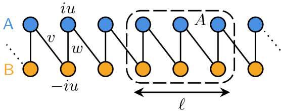
Figure 1: Schematic representation of the non-Hermitian SSH model described by the Hamiltonian of Eq. 1. We denote by $v$ and $w$ the hopping amplitudes between the rows $\mathsf{A}$ and $\mathsf{B}$ of the ladder. The chemical potential is imaginary, $iu$ for the sites in row $\mathsf{A}$ and $-iu$ for those in row $\mathsf{B}$, breaking the Hermiticity of the model. We also consider a subsystem $A$ of length $\ell$.

As we mention in the introduction, one of the most relevant applications of non-Hermitian quantum Hamiltonians nowadays is to measurement-induced phenomena. It has been shown that the unitary time evolution of a quantum state that is subject to a protocol of repeated measurements can be effectively described by a non-Hermitian Hamiltonian in the low-rate regime of measurements. In particular, in Ref. [113], the unitary evolution is generated by the Hermitian SSH model ($u=0$ in Eq. (1)) while the effective dynamics that takes into account the effect of the measurements is given by Eq. (1) with $u\neq 0$; in this case, the measurement protocol yields the staggered imaginary chemical potential of Eq. (1) that breaks Hermiticity. An experimental realization of a protocol of repeated measurements has been recently reported in Ref. [114] using a superconducting quantum processor.

The Hamiltonian (1) can be diagonalized as follows. After a discrete Fourier transform,

$$\tilde{c}_{\sigma k}=\frac{1}{\sqrt{L}}\sum_{j=1}^{L}e^{ikj}c_{\sigma j},\quad k=\frac{2\pi m}{L},$$ (3)

with $m=0,\ldots,L-1$, the Hamiltonian (1) can be cast in the form

$$H =\sum_{k}\tilde{\mathbf{c}}_{k}^{\dagger}\mathcal{H}_{k}\tilde{\mathbf{c}}_{k},$$ (4)

where $\tilde{\mathbf{c}}_{k}^{\dagger}=(\tilde{c}_{\mathsf{A}k}^{\dagger},\tilde{c}_{\mathsf{B}k}^{\dagger})$ and

$$\mathcal{H}_{k}=\begin{pmatrix}iu&\eta_{k}\\ \eta_{k}^{*}&-iu\end{pmatrix},\qquad\eta_{k}=-w-ve^{-ik}.$$ (5)

If $u\neq 0$, $\mathcal{H}_{k}$ is not Hermitian but it is still diagonalizable for almost every $k$, with an exception that will be discussed later. In fact, there exists an invertible matrix $M(k)$,

$$M(k)=\left(\begin{array}[]{cc}\frac{\eta_{k}}{|\eta_{k}|}\cos(\xi_{k})&-\frac{\eta_{k}}{|\eta_{k}|}\sin(\xi_{k})\\ \sin(\xi_{k})&\cos(\xi_{k})\end{array}\right),$$ (6)

where $2\xi_{k}=\tan^{-1}(\lvert\eta_{k}\rvert/(iu))$, such that

$$\mathcal{H}_{k}=M(k)E(k)M(k)^{-1},$$ (7)

with $E(k)=\mathrm{diag}(\varepsilon_{+,k},\varepsilon_{-,k})$ and eigenvalues

$$\varepsilon_{\pm,k}=\pm\sqrt{|\eta_{k}|^{2}-u^{2}}.$$ (8)

Therefore, introducing the new creation and annihilation operators $\mathbf{f}_{k}^{\dagger}=(f_{+,k}^{\dagger},f_{-,k}^{\dagger})$ and $\mathbf{d}_{k}=(d_{+,k},d_{-,k})^{t}$,

$$\mathbf{f}^{\dagger}_{k}=\tilde{\mathbf{c}}^{\dagger}_{k}M(k)\qquad\mathbf{d}_{k}=M(k)^{-1}\tilde{\mathbf{c}}_{k},$$ (9)

the Hamiltonian (1) is diagonal in terms of them,

$$H=\sum_{k}\mathbf{f}^{\dagger}_{k}E(k)\mathbf{d}_{k}.$$ (10)

The model presents three different phases [107]. If $w-v>u$, the system is in a $PT$-unbroken phase, with real spectrum and trivial topological properties. If $-u<w-v<u$, the system is in a $PT$-broken phase, with purely imaginary spectrum. If $w-v<-u$, the system is in a $PT$-unbroken phase, with real spectrum and non-trivial topological properties. These phases are separated by two critical lines defined by $w-v=\pm u$. Along these lines, the spectrum is $\varepsilon_{\pm,k}=\pm\sqrt{2vw(1+\cos k)}$. In this case, the two bands approach $0$ as $k\to\pi$, and the eigenspaces tend to become collinear so that $\mathcal{H}_{\pi}$ is not diagonalizable: $k=\pi$ is commonly referred to as an exceptional point.

The eigenstates of the Hamiltonian (1) can be constructed in the following way. Let us introduce the set of labels of the single particle eigenstates of $H$, $\Gamma=\{+,-\}\times\{k\}$. The vacuum state $\ket{0}$ is defined as the one annihilated by $d_{p}$ for every $p\in\Gamma$ and, therefore, $H\ket{0}=0$. The right eigenstates of $H$ are then obtained by applying sequences of $f^{\dagger}_{p}$ operators to the vacuum. More precisely, let $B$ be a subset of $\Gamma$, then $\ket{B_{R}}=\prod_{p\in B}f^{\dagger}_{p}\ket{0}$ is a right eigenstate of $H$ with eigenvalue $\sum_{p\in B}\varepsilon_{p}$. Analogously, left eigenstates are constructed by applying sequences of $d_{p}$ operators to $\bra{0}$ on the right, thus $\bra{B_{L}}=\bra{0}\prod_{p\in B}d_{p}$ is a left eigenstate of $H$ with eigenvalue $\sum_{p\in B}\varepsilon_{p}$.

If the spectrum of $H$ is real, then the eigenvalues can be ordered and the notion of ground state is well defined: it is the many-body state in which all the single particle states with negative energy are occupied. We call $\ket{\psi_{R}}$ the right ground state and $\bra{\psi_{L}}$ the left ground state, which are explicitly

$$\bra{\psi_{L}}=\bra{0}\prod_{k}d_{k,-}\qquad\ket{\psi_{R}}=\prod_{k}f^{\dagger}_{k,-}\ket{0}.$$ (11)

In a non-Hermitian setting, the natural way to define the expectation value of an observable $\mathcal{O}$ in the ground state of $H$ is $\bra{\psi_{L}}\mathcal{O}\ket{\psi_{R}}$, see Ref. [115]. It follows then that the ground state density matrix is $\rho=\ket{\psi_{R}}\bra{\psi_{L}}$. Observe that, if the system is at temperature $1/\beta$, its state may be described by the Gibbs ensemble $\rho_{\beta}=e^{-\beta H}/{\rm Tr}(e^{-\beta H})$, which in the zero-temperature limit leads to $\rho=\ket{\psi_{R}}\bra{\psi_{L}}$. As shown in detail in Refs. [24, 29], this fact facilitates the study in field theories of the entanglement entropies of $\rho$ since it allows, within the path integral formalism, to straightforwardly identify the moments of the reduced density matrix with partition functions on a replicated Riemann surface or, alternatively, with correlators of twist fields.

One may consider other density matrices, such as $\ket{\psi_{R}}\bra{\psi_{R}}$, which is Hermitian, and yields a positive definite reduced density matrix and entanglement entropies. Some entanglement properties of this density matrix in the gapped regions of the Hamiltonian (1) have been examined in Ref. [110]. However, as observed in Ref. [29], the Rényi entanglement entropies are harder to compute in field theory since the connection with partition functions on a replicated surface is not as direct as in the case $\ket{\psi_{R}}\bra{\psi_{L}}$, it involves a time reversal operation that is in general a difficult problem. Since we are interested in study the universal properties of the symmetry-resolved ground state entanglement of the critical non-Hermitian SSH chain and the corresponding CFT, in the rest of the paper we take as ground state the density matrix $\rho=\ket{\psi_{R}}\bra{\psi_{L}}$. We refer the reader to Ref. [29] for a thorough discussion on the possible choices of the total density matrix in non-Hermitian systems.

A key object in our analysis of the entanglement properties of the ground state is the two-point correlation matrix $C$ with entries

$$C_{j,j^{\prime}}=\bra{\psi_{L}}\mathbf{c}^{\dagger}_{j}\mathbf{c}_{j^{\prime}}\ket{\psi_{R}},$$ (12)

where here $\mathbf{c}_{j}=(c_{\mathsf{A}j},c_{\mathsf{B}j})$. Using Eqs. (3) and (9) to express the operators $\mathbf{c}_{j}^{\dagger}$ and $\mathbf{c}_{j}$ in terms of $\mathbf{f}_{k}^{\dagger}$ and $\mathbf{d}_{k}$, one finds

$$C_{jj^{\prime}}=\frac{1}{L}\sum_{k}e^{-ik(j-j^{\prime})}\mathcal{G}(k),$$ (13)

where

$$\mathcal{G}(k)=\frac{1}{2}\left(\begin{array}[]{cc}1-\cos(2\xi_{k})&-\sqrt{\frac{\eta_{k}^{*}}{\eta_{k}}}\sin(2\xi_{k})\\ -\sqrt{\frac{\eta_{k}}{\eta_{k}^{*}}}\sin(2\xi_{k})&1+\cos(2\xi_{k})\end{array}\right).$$ (14)

Note that, due to the dimerization of the hopping amplitudes $v$, $w$, the correlation matrix $C$ presents a $2\times 2$ block structure. In the thermodynamic limit $L\to\infty$, $C$ is a block Toeplitz matrix generated by the symbol $\mathcal{G}$.

At the critical points $w-v=\pm u$, $\mathcal{G}(k)$ has a singularity at the mode $k=\pi$ and all its entries diverge as $1/\lvert k-\pi\rvert$. Hence, the correlation matrix $C$ is not well-defined. Following Refs. [30, 31], a way to deal with this divergence is to perform in Eq. (13) a small shift in the moments $k\mapsto k+\kappa/L$, with $\kappa\ll 1$. The numerical data presented in this work has been obtained taking $\kappa=10^{-7}$.

As we have pointed out in the introduction, in this paper we are interested in studying the symmetry resolution of the ground state entanglement with respect to the $U(1)$ symmetry associated with particle number conservation at criticality. Therefore, in the following, we will restrict our analysis to the critical line $u=w-v$, which separates the $PT$-unbroken and topologically trivial phase from the $PT$-broken phase.

III Symmetry-resolved entanglement

In this section, we introduce all the quantities that we will use to investigate the symmetry-resolved entanglement in the ground state of the critical non-Hermitian SSH model previously discussed.

We consider a spatial bipartition of the system $A\cup\bar{A}$ with $A$ a subset of contiguous sites of length $\ell$ as the one depicted in Fig. 1. Then the total Hilbert space factorizes into $\mathscr{H}_{A}\otimes\mathscr{H}_{\bar{A}}$. As we have seen in the previous section, the ground state density matrix is $\rho=\ket{\psi_{R}}\bra{\psi_{L}}$. The reduced density matrix that describes the state of subsystem $A$ is obtained by taking the partial trace to the complementary subsystem $\bar{A}$, $\rho_{A}=\operatorname{Tr}_{\bar{A}}(\rho)$.

In a non-Hermitian system, we have to take into account that $\rho$ is positive semi-definite, $\rho\geq 0$, but is generally not Hermitian, $\rho^{\dagger}\neq\rho$ [115]. This fact implies that $\rho_{A}$ may not be positive semi-definite. Thus the eigenvalues of $\rho_{A}$ can be negative or even complex. In any case, $\operatorname{Tr}(\rho)=\operatorname{Tr}(\rho_{A})=1$.

The entanglement entropy of the bipartition $A\cup\bar{A}$ is defined as

$$S(\rho_{A})=-\operatorname{Tr}(\rho_{A}\log\rho_{A}).$$ (15)

For Hermitian systems, $S(\rho_{A})$ measures the degree of entanglement between subsystems $A$ and $\bar{A}$. In particular, if the low-energy physics of the model is described by a (unitary) CFT, the entanglement entropy behaves in the thermodynamic limit as

$$S(\rho_{A})=\frac{c}{3}\log\ell+O(\ell^{0})$$ (16)

where $c$ is the central charge of the corresponding CFT [21, 22, 23].

A related family of quantities are the Rényi entanglement entropies

$$S_{n}(\rho_{A})=\frac{1}{1-n}\log\operatorname{Tr}(\rho_{A}^{n}),$$ (17)

from which is possible to recover the entanglement entropy of Eq. 15 through the limit $S=\lim_{n\to 1}S_{n}$. The scaling behaviour of the Rényi entanglement entropies for critical infinite Hermitian systems is

$$S_{n}(\rho_{A})=\frac{c}{6}\frac{n+1}{n}\log\ell+O(\ell^{0}).$$ (18)

On the other hand, in non-Hermitian systems, since $\rho_{A}$ is not positive semi-definite, the entanglement entropy (15) can be complex and ambiguous, depending on which branch of the logarithm we take. In the recent Ref. [31] a new quantity dubbed generalized entanglement entropy is introduced,

$$S^{\rm g}(\rho_{A})=-\operatorname{Tr}(\rho_{A}\log\lvert\rho_{A}\rvert).$$ (19)

Observe that the only difference with the usual entropy (15) is that it takes the logarithm of $|\rho_{A}|$ instead of $\rho_{A}$: if $\rho_{A}$ is diagonalized by the matrix $R$ such that $\rho_{A}=R^{-1}{\rm diag}(\lambda_{j})R$, then $|\rho_{A}|\coloneqq R^{-1}{\rm diag}(|\lambda_{j}|)R$. This guarantees that $S^{\mathrm{g}}$ is real when the eigenvalues of $\rho_{A}$ are either negative or complex in conjugate pairs. Note that, when $\rho_{A}\geq 0$, it reduces to the standard entanglement entropy, $S^{\mathrm{g}}(\rho_{A})=S(\rho_{A})$. Although $S^{\rm g}(\rho_{A})$ can be negative, and its interpretation as an entanglement measure is not clear, it satisfies that $S^{\rm g}(\rho_{A})\neq 0$ only if the subsystems $A$ and $\bar{A}$ are entangled. Moreover, analogously to the standard entanglement entropy, it may be useful to extract information about the (non-unitary) CFTs that describe critical non-Hermitian systems. In fact, in Ref. [31], it has been verified for a set of critical non-Hermitian models, including the non-Hermitian SSH, that $S^{\rm g}(\rho_{A})$ scales as the R.H.S. of Eq. 16, even when the central charge of the associated CFT is negative. In Ref. [116], the generalized entanglement entropy (19) has been employed to study the entanglement of typical eigenstates of non-Hermitian systems and get a non-Hermitian analogue of the Page curve.

Together with the generalized entanglement entropy, one can introduce the generalized Renyi entropies

$$S_{n}^{\mathrm{g}}(\rho_{A})=\frac{1}{1-n}\log\operatorname{Tr}\left(\rho_{A}\lvert\rho_{A}\rvert^{n-1}\right)$$ (20)

that satisfy $S^{g}=\lim_{n\to 1}S_{n}^{\mathrm{g}}$.

Using the generalized entanglement entropy (19), we can extend the notion of symmetry-resolved entanglement [37, 38, 39] to non-Hermitian systems. Let us assume that the system has an internal $U(1)$ symmetry generated by a charge operator $Q$, which in our case will be the particle number operator of Eq. 2. This operator can be decomposed as the sum of the charge in $A$ and $\bar{A}$, $Q=Q_{A}+Q_{\bar{A}}$. If the left and the right ground states $\ket{\psi_{R}}$ and $\bra{\psi_{L}}$ are eigenstates of $Q$, as occurs in the non-Hermitian SSH model, then $\rho=\ket{\psi_{R}}\bra{\psi_{L}}$ commutes with $Q$. This implies that $\rho_{A}$ acts separately on each eigenspace of $Q_{A}$. Let us denote by $\Pi_{q}$ the projector onto the eigenspace of $Q_{A}$ with eigenvalue $q\in\mathbb{Z}$, also called charge sector. We then can construct a density matrix $\rho_{A,q}$ for each charge sector,

$$\rho_{A,q}=\frac{\Pi_{q}\rho_{A}\Pi_{q}}{p(q)},$$ (21)

where $p(q)=\operatorname{Tr}(\Pi_{q}\rho_{A})$ normalizes it to $\operatorname{Tr}(\rho_{A,q})=1$, such that

$$\rho_{A}=\bigoplus_{q}p(q)\rho_{A,q}.$$ (22)

In Hermitian systems, $p(q)$ is interpreted as the probability of finding the subsystem $A$ in the sector with charge $q$. However, now $\rho_{A}$ is not positive definite, so $p(q)$ may be negative, as well as larger than $1$. Hence the interpretation of $p(q)$ as a probability is lost in the non-Hermitian case.

Applying Eq. 22, the generalized entanglement entropy (19) admits the following decomposition in the charge sectors of $Q_{A}$,

$$S^{\mathrm{g}}(\rho_{A})=-\sum_{q}p(q)\log\lvert p(q)\rvert+\sum_{q}p(q)S^{\mathrm{g}}(\rho_{A,q}).$$ (23)

In the Hermitian case, the first term on the right hand side is commonly referred as the number entropy while the second is called configurational entropy [45, 46, 32].

The symmetry-resolved Rényi entanglement entropies $S^{\mathrm{g}}(\rho_{A,q})$ can be calculated using the Fourier representation of the projector $\Pi_{q}$. In fact, introducing the absolute charged moments of $\rho_{A}$

$$Z^{\mathrm{g}}_{n}(\alpha)=\operatorname{Tr}\left(\rho_{A}\lvert\rho_{A}\rvert^{n-1}e^{i\alpha Q_{A}}\right)$$ (24)

and their Fourier transform

$$\mathcal{Z}^{\mathrm{g}}_{n}(q)\coloneqq\operatorname{Tr}\left(\Pi_{q}\rho_{A}\lvert\rho_{A}\rvert^{n-1}\right)=\int_{-\pi}^{\pi}\frac{d\alpha}{2\pi}e^{-i\alpha q}Z^{\mathrm{g}}_{n}(\alpha),$$ (25)

it is possible to express all the ingredients of Eq. 23 in the form $p(q)=\mathcal{Z}^{\mathrm{g}}_{1}(q)$ and

$$S^{\mathrm{g}}_{n}(\rho_{A,q})=\frac{1}{1-n}\log\frac{\mathcal{Z}^{\mathrm{g}}_{n}(q)}{\mathcal{Z}^{\mathrm{g}}_{1}(q)\lvert\mathcal{Z}^{\mathrm{g}}_{1}(q)\rvert^{n-1}}.$$ (26)

When $\rho_{A}$ is positive definite, $Z_{n}^{\rm g}(\alpha)$ is equal to the usual charged moments of $\rho_{A}$,

$$Z_{n}(\alpha)=\operatorname{Tr}\left(\rho_{A}^{n}e^{i\alpha Q_{A}}\right).$$ (27)

In quadratic fermionic chains, the moments $Z_{n}(\alpha),Z_{n}^{\mathrm{g}}(\alpha)$ as well the whole reduced density matrix $\rho_{A}$ are accessible through the two-point correlation matrix of Eq. 12 restricted to the subsystem $A$. This result was initially derived for Hermitian systems [117] but it also holds in the non-Hermitian case [110]. Since the Hamiltonian is quadratic, then the ground state reduced density matrix satisfies the Wick theorem and, therefore, it is in general a Gaussian operator of the form $\rho_{A}=e^{-H^{\mathrm{E}}}/\mathcal{N}$, with $H^{\mathrm{E}}=\sum_{ij}c^{\dagger}_{i}\mathcal{H}^{\mathrm{E}}_{ij}c_{j}$. The relation with the two-point correlation matrix is set by

$$H^{\mathrm{E}}=\log\left[(I-C_{A}^{t})/C_{A}^{t}\right]$$ (28)

and $\mathcal{N}^{-1}=\det(I-C_{A})$, where $C_{A}$ is the restriction of $C$ to subsystem $A$, and the superscript $t$ indicates transposition. Denoting by $\nu_{j}$ the eigenvalues of $C_{A}$, it follows that

$$\log Z^{\mathrm{g}}_{n}(\alpha)=\sum_{j=1}^{2\ell}\log\left[\nu_{j}|\nu_{j}|^{n-1}e^{i\alpha}+(1-\nu_{j})|1-\nu_{j}|^{n-1}\right]$$ (29)

and

$$S^{\mathrm{g}}(\rho_{A})=-\sum_{j=1}^{2\ell}\left[\nu_{j}\log|\nu_{j}|+(1-\nu_{j})\log|1-\nu_{j}|\right].$$ (30)

The standard quantities $Z_{n}(\alpha)$ and $S(\rho_{A})$ follow analogue formulae without the absolute values. In particular,

$$\log Z_{n}(\alpha)=\sum_{j=1}^{2\ell}\log\left[\nu_{j}^{n}e^{i\alpha}+(1-\nu_{j})^{n}\right].$$ (31)

IV Absolute charged moments: the $bc$-ghost CFT

In this section, we obtain the absolute charged moments $Z_{n}^{\rm g}(\alpha)$, defined in Eq. 24, in the ground state of the non-Hermitian SSH model along the critical line $u=w-v$. To this end, we study them both numerically using Eq. (29) and analytically by considering the non-unitary CFT that describes the model at criticality.

On the critical line $u=w-v$, the low-energy physics of the non-Hermitian SSH model of Eq. 1 is captured by the $bc$-ghost CFT with central charge $c=-2$, see Ref. [30]. The action of this theory reads [118, 119]

$$S_{bc}=\int d^{2}z(\psi_{b}\bar{\partial}\psi_{c}+\bar{\psi}_{b}\partial\bar{\psi}_{c}),$$ (32)

where $\psi_{b}(z)$ and $\psi_{c}(z)$ are anti-commuting holomorphic primary fields with conformal weights $h_{b}=1$ and $h_{c}=0$ respectively, while $\bar{\psi}_{b}(\bar{z})$ and $\bar{\psi}_{c}(\bar{z})$ denote their anti-holomorphic counterparts.

The $bc$-ghost CFT has a global $U(1)$ symmetry associated to ghost number conservation, which on the lattice corresponds to the particle number of Eq. 2. The holomorphic Noether current is

$$j(z)=-:\psi_{b}(z)\psi_{c}(z):.$$ (33)

To determine the universal terms of the different moments of $\rho_{A}$ introduced in Sec. III, we consider the orbifold theory ${\rm CFT}^{\otimes n}/\mathbb{Z}_{n}$, obtained by taking $n$ copies on the complex plane of the CFT under study and then quotient the resulting tensor product by the $\mathbb{Z}_{n}$ symmetry related to the the cyclic permutation of the replicas.

Before proceeding, it is important to remark that we are assuming that the CFT is defined in the complex plane, which corresponds to taking an infinite system, i.e. $L\to\infty$, while the numerical calculations are done for a finite chain with periodic boundary conditions. In CFT, a finite periodic system is obtained by conformally mapping the complex plane to a cylinder. Since the moments of $\rho_{A}$ are given by correlators of primary fields, the effect of this map in the expression for the moments of $\rho_{A}$ is simply to replace the subsystem length $\ell$ by the chord length

$$\ell_{\mathrm{e}}=\frac{2L}{\pi}\sin\left(\frac{\pi\ell}{L}\right).$$ (34)

The factor 2 is due to the number of sites that in the full SSH chain and in the subsystem $A$ is $2L$ and $2\ell$ respectively.

In unitary CFTs, the ground state neutral moments $Z_{n}(0)=\operatorname{Tr}(\rho_{A}^{n})$ are given by the two-point correlation function of the orbifold [22, 23, 120]

$$Z_{n}(0)=\bra{0}\tau_{n}(0)\tilde{\tau}_{n}(\ell)\ket{0}.$$ (35)

Here $\ket{0}$ denotes the conformal vacuum, i.e. the state of the CFT invariant under global conformal transformations, and the fields $\tau_{n}$, $\tilde{\tau}_{n}$ are called twist and anti-twist fields [122, 121]. The winding around the point where $\tau_{n}$ ($\tilde{\tau}_{n}$) is inserted takes a field $\mathcal{O}_{k}$ living in the copy $k$ of the orbifold into the copy $k+1$ ($k-1$), for example

$$\mathcal{O}_{k}(e^{2\pi i}z)\tau_{n}(0)=\tau_{n}(0)\mathcal{O}_{k+1}(z).$$ (36)

The twist and anti-twist fields are spinless primaries with conformal dimension

$$h_{n}^{\tau}=\frac{c}{24}\left(n-\frac{1}{n}\right)$$ (37)

and, therefore, Eq. 35 directly gives Eq. 18 for the ground state Rényi entanglement entropy of Hermitian systems at the critical point.

In non-unitary CFTs, the previous discussion is more subtle because the physical ground state is not the conformal vacuum $\ket{0}$. In general, the physical ground state corresponds to the lowest eigenstate of the Virasoro operator $L_{0}$. In unitary CFTs, such eigenstate is the conformal vacuum since all the non-trivial primary fields have positive conformal dimension. On the contrary, in non-unitary CFTs, we can find primary fields with negative dimension. This implies that the ground state is the state $\ket{\phi}=\phi(0)\ket{0}$ associated to the primary $\phi$ with the lowest dimension $h_{\phi}\leq 0$. In Refs. [24, 25], it was proposed that in such case the ground state neutral moments are given by the orbifold two-point correlations

$$Z_{n}(0)=\frac{\bra{0}\tau_{n}^{\phi}(0)\tilde{\tau}_{n}^{\phi}(\ell)\ket{0}}{\bra{0}\phi(0)\phi(\ell)\ket{0}^{n}},$$ (38)

involving the composite field $\tau_{n}^{\phi}\equiv\tau_{n}\cdot\phi$, which is a spinless primary field of the orbifold with dimension

$$h_{n}^{\tau^{\phi}}=h_{n}^{\tau}+\frac{h_{\phi}}{n}.$$ (39)

Therefore, Eq. 38 implies the following behaviour for $Z_{n}(0)$ in terms of the subsystem size $\ell$

$$Z_{n}(0)\sim\ell^{-\frac{c_{\rm eff}}{6}\left(n-\frac{1}{n}\right)},$$ (40)

where $c_{\rm eff}=c-24h_{\phi}$. In the case of the $bc$-ghost theory, the lowest dimension field $\phi$ is $\psi_{c}$, which has dimension $h_{c}=0$, and then one may conclude that, in this case, $c_{\rm eff}=c=-2$.

However, the numerical analysis of the moments $Z_{n}(0)$ in the ground state of the non-Hermitian SSH model reveals that they do not behave as expected from Eq. 40 for any integer $n$ but as

$$\log Z_{n}(0)=\left\{\begin{array}[]{ll}\frac{1}{3}\left(n-\frac{1}{n}\right)\log\ell+O(\ell^{0})&n\text{ odd},\\ \\ \left(\frac{n}{3}+\frac{1}{6n}\right)\log\ell+O(\ell^{0})&n\text{ even}.\end{array}\right.$$ (41)

In fact, in the upper panel of Fig. 2, we numerically study $\log Z_{n}(0)$ as a function of the subsystem length, taking $\ell=L/2$ and varying the total system size for several values of $n$. The points are the exact numerical value of $\log Z_{n}(0)$ for the non- Hermitian SSH model obtained by diagonalizing the correlation matrix (12) and applying Eq. 31. The continuous lines correspond to Eq. 41.

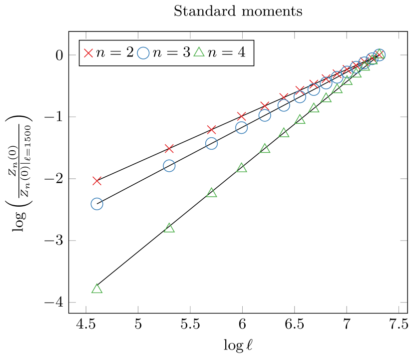
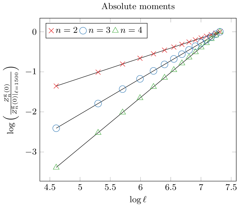
Figure 2: Standard moments $Z_{n}(0)$ (upper panel) and absolute moments $Z_{n}^{\rm g}(0)$ (lower panel) of $\rho_{A}$ as a function of the subsystem size $\ell$ and different values of the exponent $n$. We plot the ratio with the corresponding value for $\ell=1500$, taken as an arbitrary reference point. The symbols are their exact numerical value for the non-Hermitian SSH chain of length $L=\ell/2$ and parameters $w=3/2$, $v=1$ and $u=1/2$, computed through the two-point correlation matrix (13) using Eq. (31) for $Z_{n}(0)$ and Eq. (29) for $Z_{n}^{\rm g}(0)$. The solid lines correspond to the analytic expressions (41) in the upper panel and  (42) in the lower one, upon replacing $\ell$ by the chord length $\ell_{\rm e}$.

On the other hand, as the lower panel of Fig. 2 shows, we find that the absolute moments $Z_{n}^{\rm g}(0)={\rm Tr}(\rho_{A}|\rho_{A}|^{n-1})$ do follow the behaviour of Eq. 40 for any $n$,

$$\log Z_{n}^{\rm g}(0)=\frac{1}{3}\left(n-\frac{1}{n}\right)\log\ell+O(\ell^{0}),$$ (42)

as also has been numerically checked in Ref. [31]. In Fig. 2, the points are the exact numerical value of $\log Z_{n}^{\rm g}(0)$ taking as subsystem length $\ell=L/2$ and varying $L$ for several Rényi indices $n$. They have been calculated using the two-point correlation matrix (12) through Eq. 29. The continuous lines correspond to Eq. 42.

The previous analysis leads to conclude that, in the case of the $bc$-ghost theory, the ground state absolute moments of $\rho_{A}$ are given by the orbifold correlation function

$$Z_{n}^{\rm g}(0)=\bra{0}\tau_{n}(0)\tilde{\tau}_{n}(\ell)\ket{0}.$$ (43)

In Sec. VI, we will see that the alternating behavior in $n$ of the standard moments in Eq. 41 originates from the property that the eigenvalues of $\rho_{A}$ have constant sign in each charge sector and this sign depends on the parity of the charge. Combining this property and Eq. (43), we will determine the twist field correlation function that gives the correct result for $n$ even in Eq. (41).

The absolute charged moments $Z_{n}^{\rm g}(\alpha)$ of Eq. 24 can also be calculated using the orbifold ${\rm CFT}^{\otimes n}/\mathbb{Z}_{n}$. In the orbifold, the operator $e^{i\alpha Q_{A}}$ has the effect of adding a phase $e^{i\alpha}$ when a charged particle moves along a closed path that crossed all the copies. This phase shift can be incorporated in the correlators by inserting a local $U(1)$ operator $\mathcal{V}_{\alpha}(z)$ that gives rise to a term $e^{i\alpha}$ when going around it. Similarly to unitary CFTs with a $U(1)$ symmetry, see Ref. [38], we can construct the composite twist field $\tau_{n,\alpha}\equiv\tau_{n}\cdot\mathcal{V}_{\alpha}$ such that, when winding around the point where it is inserted, a field $\mathcal{O}_{k}$ living in the copy $k$ is mapped to the copy $k+1$ with an extra phase $e^{i\alpha/n}$,

$$\mathcal{O}_{k}(e^{2\pi i}z)\tau_{n,\alpha}(0)=e^{i\alpha/n}\tau_{n,\alpha}(0)\mathcal{O}_{k+1}(z).$$ (44)

If $\mathcal{V}_{\alpha}$ is a spinless primary field with conformal dimension $h_{\alpha}^{\mathcal{V}}$, then the composite twist field $\tau_{n,\alpha}$ is also a spinless primary of dimension [38]

$$h_{n,\alpha}=h_{n}^{\tau}+\frac{h_{\alpha}^{\mathcal{V}}}{n}.$$ (45)

Thus we propose that, in the $bc$-ghost theory, the absolute charged moments are given by the orbifold two-point correlation function

$$Z_{n}^{\rm g}(\alpha)=\bra{0}\tau_{n,\alpha}(0)\tilde{\tau}_{n,-\alpha}(\ell)\ket{0}.$$ (46)

Observe that this expression simplifies to Eq. 43 when $\alpha=0$.

The field $\mathcal{V}_{\alpha}$ can be determined by applying the fact that the $bc$-ghost model is equivalent via bosonization to a Gaussian theory coupled to a background charge [118]. The bosonization prescription works as follows. Let us consider a free bosonic field theory and we introduce a background charge $\mathcal{Q}$,

$$S_{\mathcal{Q}}=\frac{1}{2\pi}\int d^{2}z\left(\partial\varphi\bar{\partial}\varphi+\frac{i\mathcal{Q}}{4}\varphi\right).$$ (47)

The scalar field $\varphi(z)$ is compactified on a circle of radius one, i.e. $\varphi\sim\varphi+2\pi m$ with $m\in\mathbb{Z}$. The inclusion of a background charge in the action (47) modifies the central charge of the theory to $c=1-3\mathcal{Q}^{2}$ as well as the conformal dimension of the vertex operators $V_{\alpha}(z)=e^{i\sqrt{2}\alpha\varphi(z)}$, which is now $h_{\alpha}^{V}=\alpha^{2}-\alpha\mathcal{Q}/\sqrt{2}$. On the other hand, in presence of a background charge, $\partial\varphi$ is not a primary. If we take $\mathcal{Q}=1$, this theory has central charge $c=-2$, the fields $\psi_{b}$ and $\psi_{c}$ are identified with the vertex operators

$$\psi_{b}(z)\sim V_{-\frac{1}{\sqrt{2}}}(z),\quad\psi_{c}(z)\sim V_{\frac{1}{\sqrt{2}}}(z),$$ (48)

and the $U(1)$ current

$$j(z)=-\partial\varphi(z)$$ (49)

is equivalent to the ghost current of Eq. 33.

Therefore, using these bosonization relations, the charge operator in the interval $A$ is

$$Q_{A}=-\frac{1}{2\pi}\int_{A}dx\partial_{x}\varphi=\frac{1}{2\pi}\left(\varphi(0)-\varphi(\ell)\right),$$ (50)

and the local $U(1)$ operator $\mathcal{V}_{\alpha}$ can be identified as the vertex operator

$$\mathcal{V}_{\alpha}(z)=e^{i\frac{\alpha}{2\pi}\varphi(z)}$$ (51)

with conformal dimension

$$h_{\alpha}^{\mathcal{V}}=\frac{|\alpha|}{4\pi}\left(\frac{|\alpha|}{2\pi}-1\right).$$ (52)

Notice that such dimension is different from the standard one in the Hermitian CFT which is proportional to $\alpha^{2}$.

Finally, applying Eq. (52) in Eq. (46), we conclude that the ground state absolute charged moments of the non-Hermitian SSH model along the critical line are of the form

$$Z_{n}^{\rm g}(\alpha)=c_{n,\alpha}e^{i\alpha\langle Q_{A}\rangle}\ell^{\frac{1}{3}\left(n-\frac{1}{n}\right)-\frac{|\alpha|}{\pi n}\left(\frac{|\alpha|}{2\pi}-1\right)}.$$ (53)

Observe that in this expression we have included a phase $e^{i\alpha\langle Q_{A}\rangle}$, which depends on the average charge $\langle Q_{A}\rangle$ in the subsystem $A$. This term is not captured by the previous CFT calculations since it depends on the particular microscopical model under consideration. In the critical non-Hermitian SSH chain, the ground state is half-filled, see Eq. 11, and $\langle Q_{A}\rangle=\ell$.

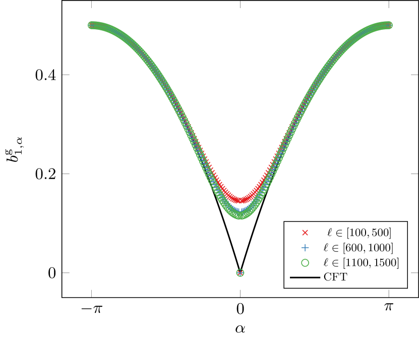
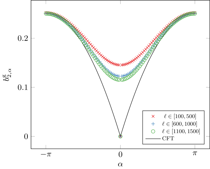
Figure 3: Numerical check of the CFT prediction (53) for the absolute charged moments $Z_{n}^{\rm g}(\alpha)$ when $n=1$ (upper panel) and $n=2$ (lower panel). As explained in the main text, the points are the value of the coefficient $b_{n,\alpha}^{\rm g}$ in Eq. (55) obtained by computing numerically $\Delta^{\rm g}$ in the non-Hermitian SSH model for several lengths $\ell$ with $L=2\ell$ at fixed $\alpha$ and then fit Eq. (55) to them. The different symbols correspond to the three sets of subsystem lengths taken to perform the fits: $\ell\in[100,500]$, $\ell\in[600,1000]$, $\ell\in[1100,1500]$, in steps of $100$. The parameters of the Hamiltonian are $w=3/2$, $v=1$, $u=1/2$. The solid line is the CFT prediction (56) for $b_{n,\alpha}^{\rm g}$.

We check numerically the result (53) in the following way. Let us define

$$\Delta^{\rm g}\coloneqq\log\frac{Z_{n}^{\rm g}(\alpha)}{Z_{n}^{\rm g}(0)}-i\alpha\langle Q_{A}\rangle.$$ (54)

According to Eq. (71), we expect

$$\Delta^{\rm g}\sim b_{n,\alpha}^{\rm g}\log\ell$$ (55)

for large $\ell$, with

$$b_{n,\alpha}^{\rm g}=-\frac{|\alpha|}{\pi n}\left(\frac{|\alpha|}{2\pi}-1\right).$$ (56)

The quantity $\Delta^{\rm g}$ can be exactly computed numerically for the ground state of the critical non-Hermitian SSH model using Eq. 29. Hence to verify that the coefficient $b_{n,\alpha}^{\rm g}$ has the form of Eq. 56, we fit the curve $b_{n,\alpha}^{\rm g}\log\ell_{\rm e}$ to a set of numerical values of $\Delta^{\rm g}$ corresponding to different subsystem sizes $\ell=L/2$ with $\alpha$ and $n$ fixed. In Fig. 3, we plot the values obtained in the fit for the coefficient $b_{n,\alpha}^{\rm g}$ in terms of $\alpha$, and compare it with the CFT prediction (56). To perform the fits, we consider three different sets of subsystem lengths, $\ell\in[100,500]$, $\ell\in[600,1000]$ and $\ell\in[1100,1500]$ in steps of $100$. For $\alpha$ large enough, there is an excellent agreement between the CFT prediction and the result of the fit. This agreement is worse as $\alpha$ decreases, while at $\alpha=0$ there is again a very good matching. Repeating the fitting procedure with each set of points, we find that the larger $\ell$ the better the agreement with the analytic result. This behaviour suggests that the convergence to Eq. 53 for large $\ell$ is not uniform in $\alpha$.

Unfortunately, the non-universal factor $c_{n,\alpha}$ cannot be determined from the CFT or applying the usual lattice techniques employed in the case of the Hermitian SSH model, i.e. corner transfer matrix, block Toeplitz determinants. Nevertheless, the numerical analysis of $c_{n,\alpha}$ reveals that the dominant term is due to the momentum shift $\kappa$, which has a simple form

$$c_{n,\alpha}\sim\begin{cases}\kappa^{1-n}&\alpha=0,\\ \kappa^{-n}&\alpha\neq 0.\end{cases}$$ (57)

V Symmetry-resolved entanglement entropy of the $bc$-ghost CFT

In this section, we use the results obtained in Eq. (53) for the absolute charged moments $Z_{n}^{\rm g}(\alpha)$ to calculate the symmetry-resolved entanglement entropy $S_{n}^{\rm g}(\rho_{A,q})$.

To this end, according to Eq. 26, we need to determine the Fourier transform of $Z_{n}^{\rm g}(\alpha)$. If we insert the CFT prediction of Eq. 53 for the absolute charged moments in Eq. 25, dropping the unknown non-universal term $c_{n,\alpha}$, then we obtain

$$\mathcal{Z}^{\mathrm{g}}_{n}(q)=(-1)^{\Delta q}Z_{n}(0)\sqrt{\frac{n\pi\ell^{\frac{1}{n}}}{2\log\ell}}e^{-\frac{n\pi^{2}\Delta q^{2}}{2\log\ell}}\\ \times\operatorname{Re}\operatorname{Erf}\left(\frac{\log\ell+i\pi n\Delta q}{\sqrt{2n\log\ell}}\right),$$ (58)

with $Z_{n}(0)=\ell^{1/3(n-1/n)}$ and $\Delta q=q-\langle Q_{A}\rangle$.

For large $\log\ell$, the error function has the asymptotic form $\operatorname{Erf}(x)\sim 1-e^{-x^{2}}/(\sqrt{\pi}x)$ and, therefore, Eq. (58) can be expanded as

$$\mathcal{Z}^{\mathrm{g}}_{n}(q)~{}\sim Z_{n}(0)\left[(-1)^{\Delta q}\sqrt{\frac{n\pi\ell^{\frac{1}{n}}}{2\log\ell}}e^{-\frac{n\pi^{2}\Delta q^{2}}{2\log\ell}}\right.\\ \left.-\frac{n\log\ell}{(\log\ell)^{2}+(n\pi\Delta q)^{2}}\right].$$ (59)

Observe the leading term in $\ell$ is a Gaussian with an alternating sign $(-1)^{\Delta q}$, while the subleading one has Lorentzian form. It is important to not neglect this term, because it is a correction only for fixed $|\Delta q|\ll\log\ell$, while it becomes leading in the regime $|\Delta q|\gtrsim\log\ell$. To understand this crossover, let us focus on the case $n=1$ which gives the normalization term $p(q)=\mathcal{Z}_{1}^{\rm g}(q)$ in the charge sector decomposition (22) of $\rho_{A}$,

$$p(q)~{}\sim(-1)^{\Delta q}\sqrt{\frac{\pi\ell}{2\log(\ell)}}e^{-\frac{\pi^{2}\Delta q^{2}}{2\log\ell}}-\frac{\log\ell}{(\log\ell)^{2}+(\pi q)^{2}}.$$ (60)

Since $p(q)=\operatorname{Tr}\left(\Pi_{q}\rho_{A}\right)$, this quantity must satisfy $\sum_{q}p(q)=1$. To get this, we have actually to take into account the two terms of Eq. (60). One can check that

$$\sum_{q\in\mathbb{Z}}p(q)=\sqrt{\frac{\pi\ell}{2\log\ell}}\vartheta_{4}(e^{-\pi^{2}/(2\log\ell)})-\frac{\ell^{2}+1}{\ell^{2}-1},$$ (61)

where the first term comes from the Gaussian in Eq. (60) and the second one from the Lorentzian. Expanding for large $\ell$, which is the only regime where the above equation makes sense (using $\vartheta_{4}(e^{-x})\sim 2\sqrt{\pi}e^{-\pi^{2}/(4x)}/\sqrt{x}$ for $x\sim 0$), we find that Eq. (61) tends to one in the large $\ell$ limit, but the Gaussian alone would provide $2$ and $-1$ comes from the Lorentzian. It is then clear that both terms should be always taken into account.

Another interesting property of Eq. (59) is that, for large $\ell$, the sign of $\mathcal{Z}_{n}^{\rm g}(q)$ is $(-1)^{\Delta q}$. In particular, in the case $n=1$, this means that the sum of the eigenvalues of $\rho_{A}$ in each charge sector of the $bc$-ghost theory has sign $(-1)^{\Delta q}$ (as long as $|\Delta q|\lesssim\log\ell$). The presence of this alternating sign can be understood by the relation

$$\rho_{A}=(-1)^{Q_{A}-\langle Q_{A}\rangle}\lvert\rho_{A}\rvert.$$ (62)

This identity can be derived in the lattice for any subsystem of arbitrary length $\ell$. In fact, along the critical line $u=w-v$, half of the eigenvalues $\nu_{j}$ of two-point correlation matrix $C_{A}$ of Eq. 12 are $\nu_{j}<0$ and the other half $\nu_{j}>1$. Given the relation (28) between the two-point correlation matrix and single particle entanglement Hamiltonian $H^{\rm E}$, the eigenvalues $\varepsilon_{j}$ of the latter are complex

$$\varepsilon_{j}=\log\left|\frac{1-\nu_{j}}{\nu_{j}}\right|+i\pi.$$ (63)

We can construct the eigenvalues of $\rho_{A}$ from those of $H^{\rm E}$. If we label them with the occupation numbers relative to the single particle entanglement Hamiltonian, then

$$\lambda_{\{n_{j}\}}=\mathcal{N}^{-1}e^{-\sum_{j}\varepsilon_{j}n_{j}}.$$ (64)

Since $\mathcal{N}=\prod_{j=1}^{2\ell}(1-\nu_{j})$ and half of the eigenvalues $\nu_{j}$ are $\nu_{j}<0$ and the other half $\nu_{j}>1$, then $\mathcal{N}=(-1)^{\ell}|\mathcal{N}|$. Combining this with Eq. 63 and identifying $\sum_{j}n_{j}=q$ and $\langle Q_{A}\rangle=\ell$, we obtain

$$\lambda_{\{n_{j}\}}=(-1)^{q-\langle Q_{A}\rangle}|\lambda_{\{n_{j}\}}|.$$ (65)

from which Eq. 62 follows.

This result indicates that the non-positiveness of $\rho_{A}$ is due to the global sign $(-1)^{q-\langle Q_{A}\rangle}$ on each charge sector $q$. Observe that in the decomposition of Eq. 22, this factor is absorbed in the normalization $p(q)$ and, therefore, the density matrices $\rho_{A,q}$ are positive definite. This implies that the generalized entanglement entropy and the standard entanglement entropy of $\rho_{A,q}$ are equal, $S_{n}^{\rm g}(\rho_{A,q})=S_{n}(\rho_{A,q})$.

Plugging Eq. 59 into (26), we obtain that the symmetry-resolved Rényi entanglement entropy in each charge sector behaves when $\log\ell\gg 1$ as

$$S^{\mathrm{g}}_{n}(\rho_{A,q})=\frac{n+1}{6n}\log\ell-\frac{1}{2}\log\log\ell+O(\ell^{0}).$$ (66)

and, in the limit $n\to 1$,

$$S^{\mathrm{g}}(\rho_{A,q})=\frac{1}{3}\log\ell-\frac{1}{2}\log\log\ell+O(\ell^{0}).$$ (67)

Note that, contrary to the generalized entanglement entropy of the full reduced density matrix $\rho_{A}$, the symmetry-resolved entanglement entropies are positive. Moreover, the expansions of Eqs. (66) and (67) coincide with the symmetry-resolved entanglement entropies of the $1+1$ free massless Dirac fermion [38, 56]. An important property of Eqs. (66) and (67) is that they do not depend on the charge $q$: at leading order in $\ell$, the symmetry-resolved entropy is equally distributed among all the charge sectors. This feature is known as entanglement equipartition [39]. As usually happens in Hermitian systems, one should further analyze the subleading $O(\ell^{0})$ terms of Eq. 66 in order to find corrections that explicitly depend on $q$. Unfortunately, we lack the proper tools to determine the first term that breaks the equipartition.

An interesting consistency test consists in recovering the total generalized entanglement entropy plugging in the decomposition (23) in charge sectors the result of Eq. (59) for $\mathcal{Z}_{n}^{\rm g}(q)$. Unfortunately, performing the sum analytically is complicated due to the the alternating sign $(-1)^{\Delta q}$ and to the interplay of the Gaussian and Lorentzian terms. Anyhow, we have checked numerically that the sum  (23) behaves as

$$S^{\rm g}(\rho_{A})\sim-\frac{2}{3}\log\ell,$$ (68)

which is the correct result for the generalized entanglement entropy (obtained also by plugging $Z_{n}^{\rm g}(0)$ of Eq. (42) in Eq. (20) and taking the limit $n\to 1^{+}$).

VI Charged moments and standard Rényi entropies

In the previous section, we obtained that along the critical line $u=w-v$, the matrices $\rho_{A}$ and $|\rho_{A}|$ are related by Eq. 62. Here we apply this identity to understand the dependence (41) on the parity of $n\in\mathbb{Z}$ of the standard moments of $\rho_{A}$, that we numerically observed in Fig. 2.

We proceed as follows. First, in the definition  (27) of the standard charged moments $Z_{n}(\alpha)$, we split $\rho_{A}^{n}=\rho_{A}\rho_{A}^{n-1}$. Then we use Eq. 62 in the $\rho_{A}^{n-1}$ factor to relate $Z_{n}(\alpha)$ to the absolute charged moments $Z_{n}^{\rm g}(\alpha)$ (cf. Eq. (24)), obtaining

$$Z_{n}(\alpha)=e^{-i\pi(n-1)\langle Q_{A}\rangle}Z_{n}^{\rm g}(\alpha+\pi(n-1)).$$ (69)

This equality implies that

$$Z_{n}(\alpha)=\begin{cases}Z_{n}^{\mathrm{g}}(\alpha)&n\text{ odd},\\ (-1)^{\langle Q_{A}\rangle}Z_{n}^{\mathrm{g}}(\alpha+\pi)&n\text{ even}.\end{cases}$$ (70)

Employing the analytic expression obtained in Eq. 53 for $Z_{n}^{\rm g}(\alpha)$, we find that, for large subsystem lengths $\ell$,

$$Z_{n}(\alpha)=\begin{cases}c_{n,\alpha}e^{i\alpha\langle Q_{A}\rangle}\ell^{\frac{1}{3}\left(n-\frac{1}{n}\right)-\frac{|\alpha|}{\pi n}\left(\frac{|\alpha|}{2\pi}-1\right)}&n\text{ odd},\\ c_{n,\alpha+\pi}e^{i\alpha\langle Q_{A}\rangle}\ell^{\frac{n}{3}+\frac{1}{6n}-\frac{\alpha^{2}}{2n\pi^{2}}}&n\text{ even}.\end{cases}$$ (71)

Note that, for $\alpha=0$, this result leads to the expressions conjectured in Eq. 41 for the neutral moments of $\rho_{A}$. In Eq. 46, we write the absolute charged moments of $\rho_{A}$ in the $bc$-ghost CFT as a correlation function of the composite twist fields $\tau_{n,\alpha}$ and $\tilde{\tau}_{n,-\alpha}$. In the light of Eq. (71), the standard charged moments are also given for $n$ odd by the same correlator, while for $n$ even we have to perform a shift in the phase $\alpha\mapsto\alpha+\pi$,

$$Z_{n}(\alpha)=\begin{cases}\bra{0}\tau_{n,\alpha}(0)\tilde{\tau}_{n,-\alpha}(\ell)\ket{0}&n\text{ odd},\\ \bra{0}\tau_{n,\alpha+\pi}(0)\tilde{\tau}_{n,-\alpha-\pi}(\ell)\ket{0}&n\text{ even}.\end{cases}$$ (72)

It is interesting to comment that the sensitivity of $Z_{n}(\alpha)$ to the parity of the exponent $n$ resembles the result for the entanglement negativity in Hermitian systems. The negativity is an entanglement measure for mixed states that can be obtained from the moments of the partial transpose of a given reduced density matrix [123]. As for our density matrix $\rho_{A}$, the partial transpose in Hermitian systems is in general non-positive definite and, in unitary CFTs, its moments also display a dependence on the parity of $n$, similar to Eq. 71, although with a different power law in $\ell$ [123, 124].

The results of Eq. (71) for the standard charged moments can be checked with exact numerical calculations in the critical non-Hermitian SSH model by following the same strategy as for the absolute charged moments presented in Sec. IV. In fact, we consider the quantity

$$\Delta\coloneqq\log\frac{Z_{n}(\alpha)}{Z_{n}(0)}-i\alpha\langle Q_{A}\rangle,$$ (73)

which according to Eq. (71), should behave as

$$\Delta\sim b_{n,\alpha}\log\ell$$ (74)

with

$$b_{n,\alpha}=\begin{cases}-\frac{|\alpha|}{\pi n}\left(\frac{|\alpha|}{2\pi}-1\right)&n\text{ odd},\\ -\frac{\alpha^{2}}{2\pi n^{2}}&n\text{ even}.\end{cases}$$ (75)

We can exactly calculate $\Delta$ in the non-Hermitian SSH model using Eq. (31). We therefore obtain numerically its value for several subsystem lengths, with $\alpha$ and $n$ fixed, and we fit the function $b_{n,\alpha}\log\ell_{\rm e}$ to them. In Fig. 4, we show the outcome for the coefficient $b_{n,\alpha}$ in the fit as a function of $\alpha$ and two particular values of $n$, $n=1$ (upper panel) and $n=2$ (lower panel). The different symbols in the plot correspond to different sets of subsystem lengths chosen to perform the fit. The continuous black curves are the analytic prediction of Eq. 75 for large $\ell$. Observe that, as we have found in Eq. 69, there is relative phase shift $\alpha\leftrightarrow\alpha+\pi$ between $n$ even and odd, consequence of the form (62) of the reduced density matrix. Similarly to the absolute charged moments, cf. Fig. 3, the figure shows that the convergence to the asymptotic expression is not uniform in $\alpha$ and worsens when approaching the cusp.

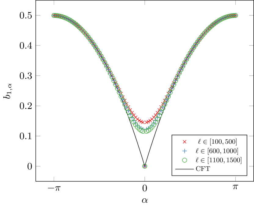
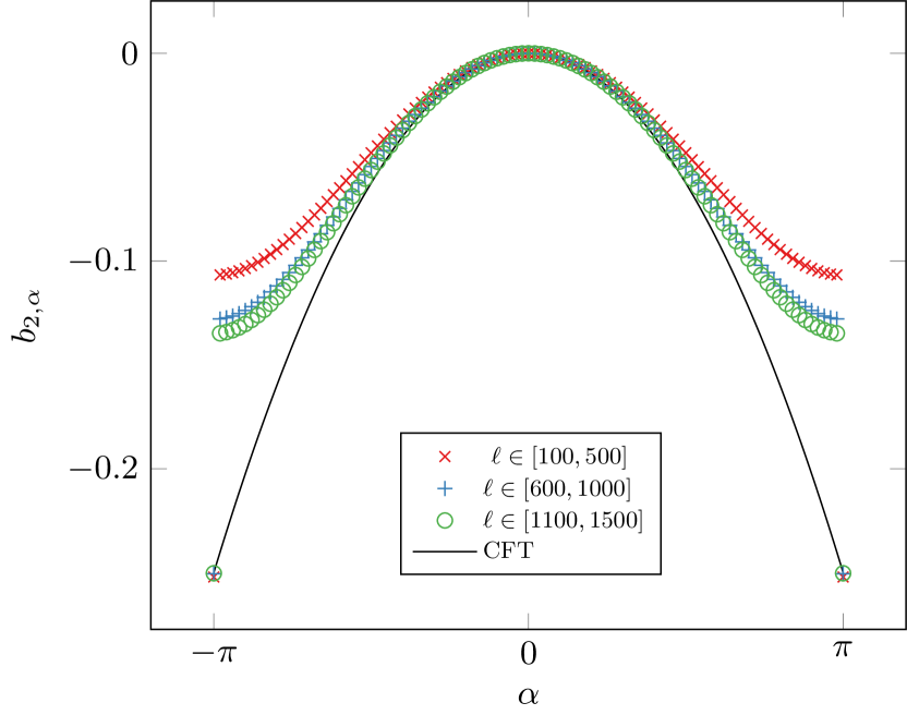
Figure 4: Numerical check of the analytic expression of Eq. (71) for the standard charged moments $Z_{n}(\alpha)$, with $n=1$ (upper panel) and $n=2$ (lower panel). As explained in the main text, the symbols are the results obtained for the coefficient $b_{n,\alpha}$ in a fit of Eq. (73) to a set of values of $\Delta$ computed numerically in the non-Hermitian SSH model and corresponding to different subsystem lengths ($\ell\in[100,500]$, $\ell\in[600,1000]$ and $\ell\in[1100,1500]$ in steps of 100) for a given $\alpha$. The parameters of the Hamiltonian are $w=3/2$, $v=1$, $u=1/2$. The solid curves are the analytic prediction of Eq. (75) for $b_{n,\alpha}$ and large subsystem size.

The oscillation in $n$ of the moments of $\rho_{A}$ implies that the standard Rényi entanglement entropies also present such behaviour. From Eq. 71, we straightforwardly get

$$S_{n}(\rho_{A})=\begin{cases}-\frac{1}{3}\left(1+\frac{1}{n}\right)\log\ell+O(\ell^{0})&n\text{ odd},\\ \frac{1}{1-n}\left(\frac{n}{3}+\frac{1}{6n}\right)\log\ell+O(\ell^{0})&n\text{ even}.\end{cases}$$ (76)

Finally, note that if we apply in the definition (15) of the standard von Neumann entanglement entropy the relation (62) between $\rho_{A}$ and $|\rho_{A}|$, and we take into account that $\langle Q_{A}\rangle=\operatorname{Tr}(\rho_{A}Q_{A})$, we find that it coincides in this case with the generalized one,

$$S(\rho_{A})=S^{\rm g}(\rho_{A})\sim-\frac{2}{3}\log\ell.$$ (77)

This asymptotic behaviour can be also extracted by taking the limit $n\to 1^{+}$ in the expression  (76) of the standard Rényi entropies for $n$ odd. This result agrees with the one obtained in Refs. [30, 27] for this quantity. However, to our knowledge, the alternating behaviour in $n$ given by Eq. (76) of the standard Rényi entropies has not been reported in previous works.

VII Entanglement spectrum

Using the results obtained in the previous section for the moments of the reduced density matrix $\rho_{A}$, we can investigate the distribution $P(\lambda)$ of the its eigenvalues, that is of the entanglement spectrum. This is defined as

$$P(\lambda)=\sum_{j}\delta(\lambda-\lambda_{j}),$$ (78)

where $\lambda_{j}$ are the eigenvalues of $\rho_{A}$. In Ref. [112], the distribution $P(\lambda)$ was determined for unitary CFTs from the knowledge of the moments $Z_{n}(0)$. That approach was extended to analyze the negativity spectrum, i.e. the eigenvalues of the partial transpose of a density matrix, in unitary CFTs [125] and free fermions [126]. As we already pointed out, the moments of $\rho_{A}$ in our non-Hermitian system present the same qualitative dependence on the parity of the exponent $n$ as the moments of the partial transpose in unitary CFTs. We can therefore easily apply here the techniques of Ref. [125] to obtain $P(\lambda)$ in the ground state of the non-Hermitian SSH model at criticality, which is the entanglement spectrum of the $bc$-ghost CFT.

The main idea of Ref. [112], and also [125], is that the distribution $P(\lambda)$ is univocally determined by its moments

$$Z_{n}(0)=\sum_{j}\lambda_{j}^{n}=\int d\lambda P(\lambda)\lambda^{n}.$$ (79)

In fact, the Stieltjes transform $f(s)$ of $\lambda P(\lambda)$,

$$f(s)=\frac{1}{\pi}\sum_{n=1}^{\infty}Z_{n}(0)s^{-n}=\frac{1}{\pi}\int d\lambda\frac{\lambda P(\lambda)}{s-\lambda},$$ (80)

is an analytic function in the complex plane except along the support of $\lambda P(\lambda)$ on the real line, where it has a branch cut. The discontinuity of $\lambda P(\lambda)$ at the branch cut gives $P(\lambda)$ through the formula [127]

$$P(\lambda)=\frac{1}{\lambda}\lim_{\epsilon\to 0^{+}}f(\lambda-i\epsilon).$$ (81)

This result implies that there is a one-to-one correspondence between the Stieltjes transform $f(s)$ and the distribution $P(\lambda)$. Therefore, given that we know the form of the moments $Z_{n}(\alpha)$, the strategy is to compute the function $f(s)$ as the Laurent series of Eq. 80 and then determine $P(\lambda)$ by applying Eq. 81.

Before proceeding, it is important two emphasize two points. When checking numerically the analytic expressions that we obtain in the following, it is crucial to take into account the shift $\kappa$ in the momenta that we have to perform to regularize the two-point correlation matrix (13) of the lattice system. We recall that this shift enters in the expression (71) of the moments $Z_{n}(0)$ through the non-universal constant $c_{n,\alpha}$, whose dependence on $\kappa$ was determined in Eq. (57). The second relevant aspect is to multiply the expressions (71) of the moments $Z_{n}(0)$ by a global factor $g^{1-n}$, both for $n$ even and odd, that accounts for a possible global degeneracy of the entanglement spectrum in the non-Hermitian SSH model, as it is explained in detailed in Ref. [128] for unitary CFTs.

Including those two extra ingredients, in Appendix A, we show in detail the calculation of the Stieljes transform $f(s)$, whose final expression reads

$$f(s)=\frac{g\kappa}{2\pi}\sum_{k=0}^{\infty}\frac{(-\log\ell)^{k}}{3^{k}k!}\left[\operatorname{Li}_{k}\left(\frac{\lambda_{M}}{s}\right)-\operatorname{Li}_{k}\left(-\frac{\lambda_{M}}{s}\right)\right]\\ +\frac{g}{\pi}\sum_{k=0}^{\infty}\frac{1}{k!}\left(\frac{\log\ell}{12}\right)^{k}\operatorname{Li}_{k}\left(\frac{\lambda_{M}^{2}}{s^{2}}\right),$$ (82)

where $\operatorname{Li}_{k}(z)$ stands for the polylogarithm function and

$$\lambda_{M}=\frac{\ell^{\frac{1}{3}}}{g\kappa}$$ (83)

is the largest eigenvalue of $\rho_{A}$ for large subsystem size $\ell$. In fact, the limit $n\to\infty$ of the standard moments $Z_{n}(0)$ gives the largest eigenvalue $\lambda_{M}$ of $\rho_{A}$ such that $\lim_{n\to\infty}Z_{n}(0)^{1/n}=\lambda_{M}$. If we take $n\to\infty$ in Eq. 71, then we obtain that in our case $\lambda_{M}$ is precisely (83). Note that this limit does not depend on the parity on $n$ of the Rényi entanglement entropy in Eq. 71 and, therefore, it is well-defined.

If we plug now Eq. 82 in the inversion formula (81), we can obtain the distribution $P(\lambda)$. This requires to apply some properties of the polylogarithm $\operatorname{Li}_{k}(z)$. The reader can find a thorough description of this calculation in Appendix A. The final expression for $P(\lambda)$ is

$$P(\lambda)=g\frac{1+\kappa}{2}\delta(\lambda-\lambda_{M})+g\frac{1-\kappa}{2}\delta(\lambda+\lambda_{M})\\ +g\frac{\Theta(\lambda_{M}-|\lambda|)}{2\lambda\sqrt{\log(\lambda_{M}/|\lambda|)}}\left[-\kappa\sqrt{\frac{\log\ell}{3}}J_{1}\left(2\xi_{\ell}(\lambda)\right)\right.\\ \left.+\operatorname{sgn}(\lambda)\sqrt{\frac{\log\ell}{6}}I_{1}\left(\sqrt{2}\xi_{\ell}(\lambda)\right)\right],$$ (84)

where $J_{\nu}(z)$ and $I_{\nu}(z)$ are the Bessel and modified Bessel functions of the first kind and

$$\xi_{\ell}(\lambda)=\sqrt{\frac{\log(\ell)\log(\lambda_{M}/\lvert\lambda\rvert)}{3}}.$$ (85)

The entanglement spectrum distribution (84) presents some remarkable properties. It is reminiscent of the negativity spectrum of two intervals [125] rather than the one-interval entanglement spectrum[112] of unitary CFTs. Its support is the interval $[-\lambda_{M},\lambda_{M}]$. The delta peaks at $\lambda=\pm\lambda_{M}$ indicate that there is a finite contribution from these two eigenvalues to the (generalized) entanglement entropies. As the momentum shift $\kappa\to 0$, the contribution of the function $J_{1}$ vanishes and $P(\lambda)$ becomes an even function in $\lambda$. Observe that the constant $g$ is still undetermined, we will fix it by comparing with the numerical data of the lattice model.

A non-trivial numerical check of the correctness of Eq. 84 is to study the tail or number distribution function $n_{\ell}(\lambda)$, that is the mean number of eigenvalues larger than a given $\lambda$,

$$n_{\ell}(\lambda)=\int_{\lambda}^{\lambda_{M}}d\lambda^{\prime}P(\lambda^{\prime}).$$ (86)

Inserting Eq. 84 in this expression, we find for $\lambda>0$

$$n_{\ell}(\lambda)=\frac{g\kappa}{2}J_{0}(2\xi_{\ell}(\lambda))+\frac{g}{2}I_{0}(\sqrt{2}\xi_{\ell}(\lambda)).$$ (87)

The main feature of this result is that the number distribution admits a particular form in which the joint dependence on $\lambda$ and $\ell$ is combined through the scaling variable $\xi_{\ell}(\lambda)$ such that

$$n_{\ell}(\lambda)=n(\xi_{\ell}(\lambda)),$$ (88)

with $n(x)$ a universal function that does not depend on the subsystem size. A similar property is found in the entanglement and negativity spectrum of unitary CFTs [112, 125].

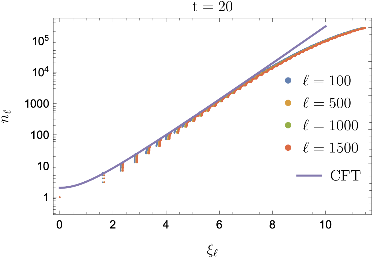
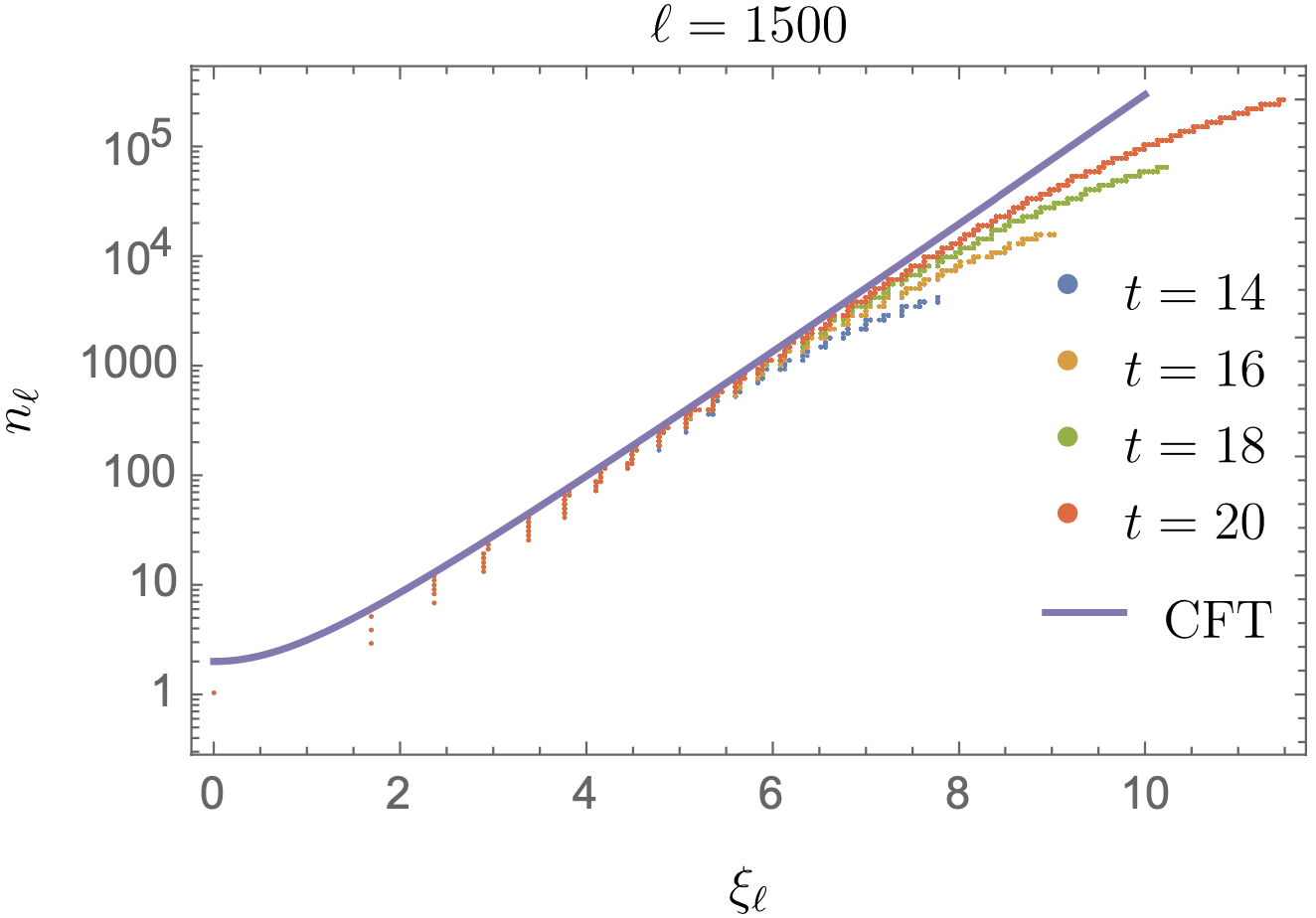
Figure 5: Number distribution of the entanglement spectrum $n_{\ell}$ as a function of the scaling variable $\xi_{\ell}$ of Eq. 85. The points have been obtained numerically as explained in the main text for the critical non-Hermitian SSH model and correspond to plot parametrically the number of eigenvalues of $\rho_{A}$ in the interval $[\lambda,\infty)$ in terms of $\xi_{\ell}(\lambda)$. In the upper panel, we consider different subsystem sizes $\ell$, truncating the spectrum of the correlation matrix to the $t=20$ largest eigenvalues. In the lower panel, we fix the subsystem size to $\ell=1500$ sites and we change the truncation to analyze its effect on the numerical results. In both panels, the solid line represents the CFT prediction for $n(\xi)$ obtained in Eqs. 87, LABEL: and 88 with $g=4$. The parameters of the Hamiltonian are $w=3/2$, $v=1$, $u=1/2$.

The structure of Eq. 88 is particularly useful when we want to make a comparison with the numerical data of the non-Hermitian SSH model. We can compute numerically the spectrum of $\rho_{A}$ for the non-Hermitian SSH model for a given subsystem length $\ell$ and plot, as we do in Fig. 5, the number of eigenvalues $\lambda_{j}$ that lie in the interval $[\lambda,\infty)$ in terms of the scaling variable $\xi_{\ell}(\lambda)$ of Eq. 85, taking as $\lambda_{M}$ the highest eigenvalue of the numerical spectrum and replacing $\ell$ by the chord length $\ell_{\mathrm{e}}$.

If we repeat this procedure for different subsystem lengths, the numerical points should converge to the CFT prediction for the number distribution of Eq. 87. In that expression, the only free term is the global factor $g$, which is still undetermined. We numerically find that the spectrum of $\rho_{A}$ for the non-Hermitian SSH model presents a global two-fold degeneracy. This forces, in particular, that the prefactor of the delta peaks in $\lambda=\pm\lambda_{M}$ of the distribution (84) must be $2$ when $\kappa\to 0$. Thus we have to take $g=4$. In Fig. 5, the solid line corresponds to (87) choosing this value for $g$. We obtain a very good agreement up to a certain value of $\xi_{\ell}(\lambda)$. In fact, for $\xi_{\ell}\to\infty$ ($\lambda\to 0$), the CFT prediction for $n_{\ell}(\lambda)$ in Eq. (87) diverges since the number of eigenvalues in the continuum is infinite. The deviation of the numerical data for large $\xi_{\ell}$ is due to the finiteness of the entanglement spectrum on the lattice and the truncation method used to obtain it numerically.

The spectrum of $\rho_{A}$ for the non-Hermitian SSH model can be determined numerically by means of the eigenvalues $\nu_{j}$ of the two-point correlation matrix, which is a $2\ell\times 2\ell$ matrix. Using Eqs. 28, LABEL: and 63, the $2^{\ell}$ eigenvalues $\lambda_{j}$ of the reduced density matrix are given by

$$\lambda_{\{n_{j}\}}=\prod_{j=1}^{2l}\nu_{j}^{n_{j}}(1-\nu_{j})^{1-n_{j}},$$ (89)

where they are labelled by a set $\{n_{j}\}$ of occupation numbers, cf. Eq. (65). Since for large $\ell$ the storage of the $2^{\ell}$ eigenvalues $\lambda_{\{n_{j}\}}$ exhausts the memory capabilities, we restrict to the eigenvalues with largest absolute value and compute them with the following approximation. We truncate the spectrum of the correlation matrix to the first $t$ eigenvalues $\nu_{j}$ that maximize the distance with respect to $0$ and $1$ and we compute $\lambda_{\{n_{j}\}}$ according to Eq. 89, with $j=1,\dots,t$. The eigenvalues $\nu_{j}$ around $0$ or $1$ would produce a multiplicative factor that is near to either $0$ or to $1$. As long as we focus on the largest eigenvalues of $\rho_{A}$, like in Fig. 5, the multiplicative factor we are missing should be close to $1$ [112]. In the upper panel of Fig. 5, we take a fixed truncation $t=20$ and consider different subsystem sizes. In the lower panel, we study the effect of the truncation for a given subsystem size; as clear from the plot, the distribution of the largest eigenvalues ($\xi_{\ell}\to 0$) is not affected when $t$ is increased.

VIII Conclusions

In this work, we have initiated the study of the symmetry resolution of entanglement in non-Hermitian systems. In particular, we have considered the generalization of the Rényi entanglement entropy based on the modulus $|\rho_{A}|$ of the reduced density matrix $\rho_{A}$ recently introduced in Ref. [31], which circumvents the problems that arise in the standard entanglement entropy due to the non-positiviness of $\rho_{A}$. Following an approach analogous to the Hermitian case [38], we have seen that the symmetry-resolved entanglement entropy can be accessed through the Fourier transform of the moments of $|\rho_{A}|$, which we have called absolute charged moments.

We have then focused on the ground state of the $bc$-ghost theory with central charge $c=-2$. This non-unitary CFT is the scaling limit of the non-Hermitian SSH model at criticality and has a global $U(1)$ symmetry. From a technical side, the main advantage of the non-Hermitian SSH model is that it is a quadratic fermionic chain, a fact that allows us to perform exact numerical calculations for large subsystem sizes thanks to Wick theorem. By applying bosonization techniques in the field theory, and with the support of exact lattice numerical calculations, we have derived the analytic expression of the absolute charged moments in the $bc$-ghost theory. They boil down to a two-point correlator of composite twist fields that properly includes the phase shift associated to the inserted charge.

From the result obtained for the absolute charged moments, we have found that the sign of the eigenvalues of $\rho_{A}$ in the $bc$-ghost CFT is determined by the charge sector to which they belong. This property is also true in the lattice system for any subsystem size. Hence, since the eigenvalues of each charge sector have equal sign, we can define a positive-definite reduced density matrix in each sector and from it a positive symmetry-resolved entanglement entropy. Interestingly, we have obtained that the symmetry-resolved entanglement entropy of the $bc$-ghost is the same as the one of the massless Dirac fermion.

We have also analytically determined the standard charged moments of $\rho_{A}$. They present different expressions when the Rényi index $n$ is either odd or even, a behaviour that stems from the dependence of the sign of the entanglement spectrum on the charge sector. This property is inherited by the standard Rényi entanglement entropies and resembles the case of the negativity in unitary CFTs [123]. To our knowledge, this feature has not been reported in the literature, but it is expected to occur if the signs of the spectrum of $\rho_{A}$ have the same charge-resolved structure as in our case. We have seen that the standard charged moments of the $bc$-ghost theory are also given by a correlator of composite twist fields with a different phase shift for $n$ even or odd.

Finally, using the results for the standard moments of $\rho_{A}$, we have analytically derived the distribution of the entanglement spectrum in the $bc$-ghost theory, which is different from that of unitary CFTs [112], although its number distribution turns out to be also a function of a scaling variable with no free parameters.

Our work leaves many open questions for future research. Here we have restricted to a particular non-unitary CFT. It would be interesting to study how our results extend to other theories or non-Hermitian systems and, in particular, to see how universal are the expressions for the symmetry-resolved entanglement entropy and the entanglement spectrum distribution that we obtain for the $bc$-ghost theory with central charge $-2$. In this respect, it would be needed a careful analysis using a path integral approach of the twist field correlators that give the (absolute) charged moments of $\rho_{A}$. Another relevant line would be to explore theories in which the spectrum of $\rho_{A}$ has other forms, e.g. it is complex, and wonder if the symmetry-resolved entropy is positive-definite as well. Moreover, here we have considered as ground state density matrix $\ket{\psi_{R}}\bra{\psi_{L}}$, but this is not the only possible choice; for example $\ket{\psi_{R}}\bra{\psi_{R}}$, whose reduced density matrix is positive definite, is another reasonable alternative. It would be nice to study the symmetry-resolved entanglement entropies in such state and compare with our results. Of course, the entanglement entropy is not the only entanglement measure that can be resolved in symmetry sectors, for example the negativity, which can be employed to study entanglement in disjoint subsystems [67, 74], or the operator entanglement [36]. One can also consider to carry out a similar analysis for them.

Acknowledgements. We thank L. Capizzi, A. Delmonte, J. Dubail, F. Essler, C. Muzzi, S. Murciano, F. Rottoli, C. Rylands, and S. Scopa for useful discussions. The authors acknowledge support from ERC under Consolidator grant number 771536 (NEMO).

Appendix A Details of the computation of $P(\lambda)$

In this appendix, we discuss in detail how to obtain the entanglement spectrum distribution $P(\lambda)$ of $\rho_{A}$ from its moments $Z_{n}(0)$ through the Stieljes transform $f(s)$.

In order to lighten the notation, let us rewrite the moments (71) of $\rho_{A}$ in the form

$$Z_{n}(0)=\begin{cases}g\kappa e^{-bn+b^{\prime}/n},&n\text{ odd},\\ ge^{-bn+b^{\prime}/(2n)},&n\text{ even},\end{cases}$$ (90)

where

$$e^{-b}=\frac{\ell^{1/3}}{g\kappa},\quad e^{b^{\prime}}=\ell^{1/3}.$$ (91)

As explained in the main text, we have assumed in Eq. (90) that the non-universal term $c_{n,\alpha}$ is of the form of Eq. (57) and we have multiplied the expressions both for $n$ even and odd by a global factor $g^{n-1}$ to take into account a possible global degeneracy of the entanglement spectrum.

According to Eq. 80, the moments of $\rho_{A}$ are the coefficients of the Laurent series expansion of $f(s)$. Taking int account the dependence of $Z_{n}(0)$ on the parity of $n$, we split the series in the form

$$f(s)=\frac{1}{\pi}\left[\sum_{n=0}^{\infty}Z_{2n+1}(0)s^{-(2n+1)}+\sum_{n=1}^{\infty}Z_{2n}(0)s^{-2n}\right].$$ (92)

Inserting Eq. 90 in this expression, and taking the Taylor series of $e^{b^{\prime}/n}$ and $e^{b^{\prime}/(2n)}$ in the odd and even terms respectively,

$$f(s) = \frac{g}{\pi}\left[\kappa\sum_{n=0}^{\infty}e^{-b(2n+1)-\frac{b^{\prime}}{2n+1}}s^{-(2n+1)}+\sum_{n=1}^{\infty}e^{-b2n+\frac{b^{\prime}}{4n}}s^{-2n}\right]$$ (93)

$$= \frac{g}{\pi}\left[\frac{\kappa e^{-b}}{s}\sum_{k=0}^{\infty}\frac{(-b^{\prime})^{k}}{k!}\sum_{n=0}^{\infty}\frac{(e^{-2b}/s^{2})^{n}}{(2n+1)^{k}}+\sum_{k=0}^{\infty}\frac{1}{k!}\left(\frac{b^{\prime}}{4}\right)^{k}\sum_{n=1}^{\infty}\frac{(e^{-2b}/s^{2})^{n}}{n^{k}}\right],$$ (94)

we can then identify the Lerch trascendent $\phi(z,\nu,\alpha)=\sum_{n=0}^{\infty}\frac{z^{n}}{(n+\alpha)^{\nu}}$ in the odd term and the polylogarithm function ${\rm Li}_{\nu}(z)=\sum_{k=1}^{\infty}z^{k}/k^{\nu}$ in the even term,

$$f(s)=\frac{g}{\pi}\left[\frac{\kappa e^{-b}}{s}\sum_{k=0}^{\infty}\frac{(-b^{\prime})^{k}}{2^{k}k!}\mathrm{\phi}(e^{-2b}/s^{2},k,1/2)+\sum_{k=0}^{\infty}\frac{1}{k!}\left(\frac{b^{\prime}}{4}\right)^{k}\operatorname{Li}_{k}\left(\frac{e^{-2b}}{s^{2}}\right)\right].$$ (95)

Finally, making use of the identity

$$2^{-k}z\phi(z^{2},k,1/2)=\frac{1}{2}\left(\operatorname{Li}_{k}(z)-\operatorname{Li}_{k}(-z)\right),$$ (96)

we arrive at Eq. 82

$$f(s)=\frac{g\kappa}{2\pi}\sum_{k=0}^{\infty}\frac{(-b^{\prime})^{k}}{k!}\left[\operatorname{Li}_{k}\left(\frac{e^{-b}}{s}\right)-\operatorname{Li}_{k}\left(-\frac{e^{-b}}{s}\right)\right]+\frac{g}{\pi}\sum_{k=0}^{\infty}\frac{1}{k!}\left(\frac{b^{\prime}}{4}\right)^{k}\operatorname{Li}_{k}\left(\frac{e^{-2b}}{s^{2}}\right).$$ (97)

Once the Stieljes transform $f(s)$ is determined, we can obtain the distribution $P(\lambda)$ using the inversion formula (81). The technical crucial point when applying Eq. 81 is that the polylogarith function ${\rm Li}_{k}(z)$ for $k\geq 1$ is a multivalued function with a branch point at $z=1$. If we take as branch cut the real interval $[1,\infty)$, the discontinuity across the cut is

$$\lim_{\epsilon\to 0^{+}}\operatorname{Im}\operatorname{Li}_{k}(y\pm i\epsilon)=\begin{cases}\pm\pi(\log y)^{k-1}/\Gamma(k)&y\geq 1\\ 0&y<1.\end{cases}$$ (98)

Using this property, we can easily obtain $P(\lambda)$ with Eqs. (81) and (97). To this end, let us consider separately the two terms of Eq. 97. We define the function

$$f^{>}_{\mathrm{odd}}(s)=\frac{g\kappa}{2\pi}\sum_{k=1}^{\infty}\frac{(-b^{\prime})^{k}}{k!}\left(\operatorname{Li}_{k}(e^{-b}/s)-\operatorname{Li}_{k}(-e^{-b}/s)\right),$$ (99)

which corresponds to the first term of Eq. 97, but removing the mode $k=0$. If we apply Eq. 98, then we find

$$\lim_{\epsilon\to 0^{+}}\operatorname{Im}f^{>}_{\mathrm{odd}}(\lambda-i\epsilon) = \frac{g\kappa\Theta(e^{-b}-\lambda)}{2\log(e^{-b}/|\lambda|)}\sum_{k=1}^{\infty}\frac{1}{k!\Gamma(k)}\left(-b^{\prime}\log\frac{e^{-b}}{|\lambda|}\right)^{k}$$ (100)

$$= -\frac{g\kappa\Theta(e^{-b}-\lambda)}{2\log(e^{-b}/|\lambda|)}\sqrt{b^{\prime}\log\frac{e^{-b}}{|\lambda|}}\,J_{1}\left(2\sqrt{b^{\prime}\log\frac{e^{-b}}{|\lambda|}}\right)$$

where $\Theta$ is the Heaviside step function and $J_{1}$ is the Bessel function of the first kind. Note that for the last equality we have used that $b^{\prime}>0$

Analogously, we define

$$f^{>}_{\mathrm{even}}(s)=\frac{g}{\pi}\sum_{k=1}^{\infty}\frac{1}{k!}\left(\frac{a}{2}\right)^{k}\operatorname{Li}_{k}\left(\frac{e^{-2b}}{s^{2}}\right),$$ (101)

which is the second term of $f(s)$ in Eq. 97 without the mode $k=0$. If we again apply here Eq. 98, we have to take into account that for small $\epsilon$, the argument of the polylogarithm in Eq. 101 behaves as

$$\frac{e^{-2b}}{(\lambda-i\epsilon)^{2}}=\frac{e^{-2b}}{\lambda^{2}}+i\epsilon 2\frac{e^{-2b}}{\lambda^{3}}+o(\epsilon^{2})$$ (102)

and, therefore, it approaches the branch cut from above or from below depending on the sign of $\lambda$. It then follows that

$$\lim_{\epsilon\to 0^{+}}{\rm Im}f^{>}_{\mathrm{even}}(\lambda-i\epsilon) = \operatorname{sign}(\lambda)\frac{g\Theta(e^{-b}-|\lambda|)}{2\log(e^{-b}/|\lambda|)}\sum_{k=1}^{\infty}\frac{1}{k!\Gamma(k)}\left(\frac{b^{\prime}}{2}\log\frac{e^{-b}}{|\lambda|}\right)^{k}$$ (103)

$$= g\Theta(e^{-b}-|\lambda|)\frac{\operatorname{sign}(\lambda)}{2\log\frac{e^{-b}}{|\lambda|}}\sqrt{\frac{b^{\prime}}{2}\log\frac{e^{-b}}{|\lambda|}}\,I_{1}\left(2\sqrt{\frac{b^{\prime}}{2}\log\frac{e^{-b}}{|\lambda|}}\right)$$

where $I_{1}$ is the modified Bessel function of the first kind and in the last equality we have used $b^{\prime}>0$.

We still have to study the modes $k=0$ of $f(s)$ in Eq. 97,

$$f_{0}(s)=\frac{g}{\pi}\operatorname{Im}\left[\frac{\kappa}{2}\operatorname{Li}_{0}\left(\frac{e^{-b}}{s}\right)-\frac{\kappa}{2}\operatorname{Li}_{0}\left(\frac{-e^{-b}}{s}\right)+\operatorname{Li}_{0}\left(\frac{e^{-2b}}{s^{2}}\right)\right].$$ (104)

Taking into account that ${\rm Li}_{0}(z)=z/(1-z)$, they can be rewritten as

$$f_{0}(s)=\frac{g}{\pi}\left[\frac{\kappa}{2}\frac{1}{s/e^{-b}-1}+\frac{\kappa}{2}\frac{1}{s/e^{-b}+1}+\frac{1}{s^{2}/e^{-2b}-1}\right].$$ (105)

Applying the Sokhotski–Plemelj formula

$$\lim_{\epsilon\to 0^{+}}\frac{1}{x\pm i\epsilon}=\mp i\pi\delta(x)+{\rm PV}\left(\frac{1}{x}\right),$$ (106)

where ${\rm PV}$ stands for the Cauchy principal value, we get

$$\lim_{\epsilon\to 0^{+}}\operatorname{Im}f_{0}(\lambda-i\epsilon)=g\lambda\frac{1+\kappa}{2}\delta(\lambda-e^{-b})+g\lambda\frac{1-\kappa}{2}\delta(\lambda+e^{-b}).$$ (107)

Finally, putting Eqs. (100), (103), and (107) together in the inversion formula (81), we get Eq. 84

$$P(\lambda)=g\frac{1+\kappa}{2}\delta(\lambda-\lambda_{M})+g\frac{1-\kappa}{2}\delta(\lambda+\lambda_{M})+\\ +g\frac{\Theta(\lambda_{M}-|\lambda|)}{2\lambda\sqrt{\log(\lambda_{M}/|\lambda|)}}\left[-\kappa\sqrt{b^{\prime}}J_{1}\left(2\sqrt{b^{\prime}\log\left(\lambda_{M}/|\lambda|\right)}\right)+\operatorname{sgn}(\lambda)\sqrt{b^{\prime}/2}I_{1}\left(2\sqrt{b^{\prime}/2\log\left(\lambda_{M}/|\lambda|\right)}\right)\right]$$ (108)

where we have used that $e^{-b}=\lambda_{M}$.

References

- [1] N. Moiseyev, Non-Hermitian Quantum Mechanics, Cambridge University Press, Cambridge (2011).
- [2] Y. Ashida, Z. Gong, and M. Ueda, Non-Hermitian Physics, Adv. Phys. 69, 3 (2020).
- [3] C. M. Bender and S. Boettcher, Real spectra in non-Hermitian Hamiltonians having PT symmetry, Phys. Rev. Lett. 80 5243 (1998).
- [4] C.M. Bender, PT-symmetric quantum theory, J. Phys. Conf. Ser. 631, 012002 (2015).
- [5] R. El-Ganainy, K. G. Makris, M. Khajavikhan, Z. H. Musslimani, S. Rotter, and D. N. Christodoulides, Non-Hermitian physics and PT symmetry, Nature Phys. 14, 11 (2018).
- [6] L. Feng, R. El-Ganainy, and L. Ge, Non-Hermitian photonics based on parity–time symmetry, Nature Photon. 11, 752 (2017).
- [7] M. A. Miri and A. Alù, Exceptional points in optics and photonics, Science 363, 6422 (2019).
- [8] E. M. Graefe, H. J. Korsch, and A. E. Niederle, Mean-Field Dynamics of a Non-Hermitian Bose-Hubbard Dimer, Phys. Rev. Lett. 101, 150408 (2008).
- [9] I. Rotter, A non-Hermitian Hamilton operator and the physics of open quantum systems, J. Phys. A: Math. Theor. 42, 153001 (2009).
- [10] M. Müller, S. Diehl, G. Pupillo, and P. Zoller, Engineered Open Systems and Quantum Simulations with Atoms and Ions, Advances in Atomic, Molecular, and Optical Physics 61, 1 (2012).
- [11] S. Gopalakrishan and M. J. Gullans, Entanglement and purification transitions in non-Hermitian quantum mechanics, Phys. Rev. Lett. 126, 170503 (2021).
- [12] A. Biella and M. Schiró, Many-Body Quantum Zeno Effect and Measurement-Induced Subradiance Transition, Quantum 5, 528 (2021).
- [13] X. Turkeshi, A. Biella, R. Fazio, M. Dalmonte, and M. Schiró, Measurement-induced entanglement transitions in the quantum Ising chain: From infinite to zero clicks, Phys. Rev. B 103, 224210 (2021).
- [14] T. Müller , S. Diehl, and M. Buchhold, Measurement-Induced Dark State Phase Transitions in Long-Ranged Fermion Systems, Phys. Rev. Lett. 128, 010605 (2022).
- [15] X. Turkeshi and M. Schirò, Entanglement and correlation spreading in non-Hermitian spin chains, Phys. Rev. B 107, L020403 (2023).
- [16] L. Amico, R. Fazio, A. Osterloh, and V. Vedral, Entanglement in many-body systems, Rev. Mod. Phys. 80, 517 (2008).
- [17] P. Calabrese, J. Cardy, and B. Doyon, Entanglement entropy in extended quantum systems, J. Phys. A 42, 500301 (2009).
- [18] N. Laflorencie, Quantum entanglement in condensed matter systems, Phys. Rep. 643, 1 (2016).
- [19] M. Rangamani and T. Takanayagi, Holographic Entanglement Entropy, Lect. Notes Phys. 931 (2017).
- [20] J. Eisert, M. Cramer, and M. B. Plenio, Area laws for the entanglement entropy, Rev. Mod. Phys. 82, 277 (2010).
- [21] C. Holzhey, F. Larsen, and F. Wilczek, Geometric and Renormalized Entropy in Conformal Field Theory, Nucl. Phys. B 424, 443 (1994).
- [22] P. Calabrese and J. Cardy, Entanglement entropy and quantum field theory, J. Stat. Mech. (2004) P06002.
- [23] P. Calabrese and J. Cardy, Entanglement entropy and conformal field theory, J. Phys. A 42, 504005 (2009).
- [24] D. Bianchini, O. A. Castro-Alvaredo, B. Doyon, E. Levi, and F. Ravanini, Entanglement Entropy of Non Unitary Conformal Field Theory, J. Phys. A: Math. Theor. 48, 04FT01 (2015).
- [25] D. Bianchini, O. A. Castro-Alvaredo, and B. Doyon, Entanglement Entropy of Non-Unitary Integrable Quantum Field Theory, Nucl. Phys. B 896, 835 (2015).
- [26] D. Bianchini and F. Ravanini, Entanglement entropy from corner transfer matrix in Forrester-Baxter non-unitary RSOS models, J. Phys. A: Math. Theor. 49, 154005 (2016).
- [27] K. Narayan, On dS4 extremal surfaces and entanglement entropy in some ghost CFTs, Phys. Rev. D 94, 046001 (2016).
- [28] R. Couvreur, J. L. Jacobsen, and H. Saleur, Entanglement in Nonunitary Quantum Critical Spin Chains, Phys. Rev. Lett. 119, 040601 (2017).
- [29] T. Dupic, B. Estienne, and Y. Ikhlef, Entanglement entropies of minimal models from null-vectors, SciPost Phys. 4, 031 (2018).
- [30] P.-Y. Chang, J.-S. You, X. Wen, and S. Ryu, Entanglement spectrum and entropy in topological non-Hermitian systems and nonunitary conformal field theory, Phys. Rev. Research 2, 033069 (2020).
- [31] Y.-T. Tu, Y.-C. Tzeng, and P.-Y. Chang, Rényi entropies and negative central charges in non-Hermitian quantum systems, SciPost Phys. 12, 194 (2022).
- [32] A. Lukin, M. Rispoli, R. Schittko, M. E. Tai, A. M. Kaufman, S. Choi, V. Khemani, J. Leonard, and M. Greiner, Probing entanglement in a many-body localized system, Science 364, 6437 (2019).
- [33] D. Azses, R. Haenel, Y. Naveh, R. Raussendorf, E. Sela, and E. G. Dalla Torre, Identification of Symmetry-Protected Topological States on Noisy Quantum Computers, Phys. Rev. Lett. 125, 120502 (2020).
- [34] A. Neven, J. Carrasco, V. Vitale, C. Kokail, A. Elben, M. Dalmonte, P. Calabrese, P. Zoller, B. Vermersch, R. Kueng, and B. Kraus, Symmetry-resolved entanglement detection using partial transpose moments, npj Quantum Info. 7, 1 (2021).
- [35] V. Vitale, A. Elben, R. Kueng, A. Neven, J. Carrasco, B. Kraus, P. Zoller, P. Calabrese, B. Vermersch, and M. Dalmonte, Symmetry-resolved dynamical purification in synthetic quantum matter, SciPost Phys. 12, 106 (2022).
- [36] A. Rath, V. Vitale, S. Murciano, M. Votto, J. Dubail, R. Kueng, C. Branciard, P. Calabrese, and B. Vermersch, Entanglement Barrier and its Symmetry Resolution: Theory and Experimental Observation, Phys. Rev. X Quantum 4, 010318 (2023).
- [37] N. Laflorencie and S. Rachel, Spin-resolved entanglement spectroscopy of critical spin chains and Luttinger liquids, J. Stat. Mech. (2014) P11013.
- [38] M. Goldstein and E. Sela, Symmetry-resolved entanglement in many-body systems, Phys. Rev. Lett. 120, 200602 (2018).
- [39] J. C. Xavier, F. C. Alcaraz, and G. Sierra Equipartition of the Entanglement Entropy, Phys. Rev. B 98, 041106 (2018).
- [40] R. Bonsignori, P. Ruggiero, and P. Calabrese, Symmetry resolved entanglement in free fermionic systems, J. Phys. A 52, 475302 (2019).
- [41] S. Murciano, G. Di Giulio, and P. Calabrese, Symmetry resolved entanglement in gapped integrable systems: a corner transfer matrix approach, SciPost Phys. 8, 046 (2020).
- [42] S. Fraenkel and M. Goldstein, Symmetry resolved entanglement: Exact results in 1d and beyond, J. Stat. Mech. (2020) 033106.
- [43] P. Calabrese, M. Collura, G. Di Giulio, and S. Murciano, Full counting statistics in the gapped XXZ spin chain, EPL 129, 60007 (2020).
- [44] H. M. Wiseman and J. A. Vaccaro, Entanglement of Indistinguishable Particles Shared between Two Parties, Phys. Rev. Lett. 91, 097902 (2003).
- [45] H. Barghathi, C. M. Herdman, and A. Del Maestro, Rényi Generalization of the Accessible Entanglement Entropy, Phys. Rev. Lett. 121, 150501 (2018).
- [46] H. Barghathi, E. Casiano-Diaz, and A. Del Maestro, Operationally accessible entanglement of one dimensional spinless fermions, Phys. Rev. A 100, 022324 (2019).
- [47] H. Barghathi, J. Yu, and A. Del Maestro Theory of noninteracting fermions and bosons in the canonical ensemble, Phys. Rev. Res. 2, 043206 (2020).
- [48] S. Murciano, P. Ruggiero, and P. Calabrese, Symmetry resolved entanglement in two-dimensional systems via dimensional reduction, J. Stat. Mech. (2020) 083102.
- [49] M. T. Tan and S. Ryu, Particle Number Fluctuations, Rényi and Symmetry-resolved Entanglement Entropy in Two-dimensional Fermi Gas from Multi-dimensional bosonisation, Phys. Rev. B 101, 235169 (2020).
- [50] Z. Ma, C. Han, Y. Meir, and E. Sela, Symmetric inseparability and number entanglement in charge conserving mixed states, Phys. Rev. A 105, 042416 (2022).
- [51] F. Ares, S. Murciano, and P. Calabrese, Symmetry-resolved entanglement in a long-range free-fermion chain, J. Stat. Mech. (2022) 063104.
- [52] N. G. Jones, Symmetry-resolved entanglement entropy in critical free-fermion chains, J. Statist. Phys. 188 (2022) 28.
- [53] L. Piroli, E. Vernier, M. Collura, and P. Calabrese, Thermodynamic symmetry resolved entanglement entropies in integrable systems, J. Stat. Mech. (2022) 073102.
- [54] C. Han, Y. Meir, and E. Sela, Realistic protocol to measure entanglement at finite temperatures, Phys. Rev. Lett. 130, 136201 (2023).
- [55] S. Murciano, P. Calabrese, and L. Piroli, Symmetry-resolved Page curves, Phys. Rev. D 106, 046015 (2022)
- [56] S. Murciano, G. Di Giulio, and P. Calabrese, Entanglement and symmetry resolution in two dimensional free quantum field theories, JHEP 08 (2020) 073.
- [57] D. X. Horvath and P. Calabrese, Symmetry resolved entanglement in integrable field theories via form factor bootstrap, JHEP 11 (2020) 131.
- [58] D. X. Horvath, L. Capizzi, and P. Calabrese, U(1) symmetry resolved entanglement in free 1+1 dimensional field theories via form factor bootstrap, JHEP 05 (2021) 197.
- [59] D. X. Horvath, P. Calabrese, and O. A. Castro-Alvaredo, Branch Point Twist Field Form Factors in the sine-Gordon Model II: Composite Twist Fields and Symmetry Resolved Entanglement, SciPost Phys. 12, 088 (2022).
- [60] L. Capizzi, D. X. Horvath, P. Calabrese, and O. A. Castro-Alvaredo, Entanglement of the 3-State Potts Model via Form Factor Bootstrap: Total and Symmetry Resolved Entropies, JHEP 05 (2022) 113.
- [61] L. Capizzi, O. A. Castro-Alvaredo, C. De Fazio, M. Mazzoni, and L. Santamaría-Sanz, Symmetry Resolved Entanglement of Excited States in Quantum Field Theory I: Free Theories, Twist Fields and Qubits JHEP 12 (2022) 127.
- [62] L. Capizzi, O. A. Castro-Alvaredo, C. De Fazio, M. Mazzoni, and L. Santamaría-Sanz, Symmetry Resolved Entanglement of Excited States in Quantum Field Theory II: Numerics, Interacting Theories and Higher Dimensions, JHEP 12 (2022) 128.
- [63] L. Capizzi, M. Mazzoni, and O. A. Castro-Alvaredo Symmetry Resolved Entanglement of Excited States in Quantum Field Theory III: Bosonic and Fermionic Negativity, arXiv:2302.02666.
- [64] M. Mazzoni and O. A. Castro-Alvaredo, Two-Point Functions of Composite Twist Fields in the Ising Field Theory, J. Phys. A: Math. Theor. 56, 124001 (2023).
- [65] E. Cornfeld, M. Goldstein, and E. Sela, Imbalance Entanglement: Symmetry Decomposition of Negativity, Phys. Rev. A 98, 032302 (2018).
- [66] L. Capizzi, P. Ruggiero, and P. Calabrese, Symmetry resolved entanglement entropy of excited states in a CFT, J. Stat. Mech. (2020) 073101.
- [67] S. Murciano, R. Bonsignori, and P. Calabrese, Symmetry decomposition of negativity of massless free fermions, SciPost Phys. 10, 111 (2021).
- [68] H.-H. Chen, Symmetry decomposition of relative entropies in conformal field theory, JHEP 07 (2021) 084.
- [69] L. Capizzi and P. Calabrese, Symmetry resolved relative entropies and distances in conformal field theory, JHEP 10 (2021) 195.
- [70] L. Hung and G. Wong, Entanglement branes and factorization in conformal field theory, Phys. Rev. D 104, 026012 (2021).
- [71] P. Calabrese, J. Dubail, and S. Murciano, Symmetry-resolved entanglement entropy in Wess-Zumino-Witten models, JHEP 10 (2021) 067.
- [72] R. Bonsignori and P. Calabrese, Boundary effects on symmetry resolved entanglement, J. Phys. A 54, 015005 (2021).
- [73] B. Estienne, Y. Ikhlef, and A. Morin-Duchesne, Finite-size corrections in critical symmetry-resolved entanglement, SciPost Phys. 10, 054 (2021).
- [74] H.-H. Chen, Charged Rényi negativity of massless free bosons, JHEP 02 (2022) 117.
- [75] A. Milekhin and A. Tajdini, Charge fluctuation entropy of Hawking radiation: a replica-free way to find large entropy, arXiv:2109.03841.
- [76] M. Ghasemi, Universal Thermal Corrections to Symmetry-Resolved Entanglement Entropy and Full Counting Statistics, arXiv:2203.06708.
- [77] F. Ares, P. Calabrese, G. Di Giulio, and S. Murciano,, Multi-charged moments of two intervals in conformal field theory, JHEP 09 (2022) 051.
- [78] A. Foligno, S. Murciano, and P. Calabrese, Entanglement resolution of free Dirac fermions on a torus, JHEP 03 (2023) 096.
- [79] G. Di Giulio, R. Meyer, C. Northe, H. Scheppach, and S. Zhao, On the Boundary Conformal Field Theory Approach to Symmetry-Resolved Entanglement, arXiv:2212.09767.
- [80] L. Capizzi, S. Murciano, and P. Calabrese, Full counting statistics and symmetry resolved entanglement for free conformal theories with interface defects, arXiv:2302.08209.
- [81] X. Turkeshi, P. Ruggiero, V. Alba, and P. Calabrese, Entanglement equipartition in critical random spin chains, Phys. Rev. B 102, 014455 (2020).
- [82] M. Kiefer-Emmanouilidis, R. Unanyan, J. Sirker, and M. Fleischhauer, Evidence for unbounded growth of the number entropy in many-body localized phases, Phys. Rev. Lett. 124, 243601 (2020).
- [83] M. Kiefer-Emmanouilidis, R. Unanyan, J. Sirker, and M. Fleischhauer, Bounds on the entanglement entropy by the number entropy in non-interacting fermionic systems, SciPost Phys 8, 083 (2020).
- [84] M. Kiefer-Emmanouilidis, R. Unanyan, M. Fleischhauer, and J. Sirker, Absence of true localization in many-body localized phases, Phys. Rev. B 103, 024203 (2021).
- [85] N. Feldman and M. Goldstein, Dynamics of Charge-Resolved Entanglement after a Local Quench, Phys. Rev. B 100, 235146 (2019).
- [86] G. Parez, R. Bonsignori, and P. Calabrese, Quasiparticle dynamics of symmetry resolved entanglement after a quench: the examples of conformal field theories and free fermions, Phys. Rev. B 103, L041104 (2021).
- [87] G. Parez, R. Bonsignori, and P. Calabrese, Exact quench dynamics of symmetry resolved entanglement in a free fermion chain, J. Stat. Mech. (2021) 093102.
- [88] S. Fraenkel and M. Goldstein, Entanglement Measures in a Nonequilibrium Steady State: Exact Results in One Dimension, SciPost Phys. 11, 085 (2021).
- [89] G. Parez, R. Bonsignori, and P. Calabrese, Dynamics of charge-imbalance-resolved entanglement negativity after a quench in a free-fermion mode, J. Stat. Mech. (2022) 053103.
- [90] S. Scopa and D. X. Horvath, Exact hydrodynamic description of symmetry-resolved Rényi entropies after a quantum quench, J. Stat. Mech. (2022) 083104.
- [91] H.-H. Chen, Dynamics of charge imbalance resolved negativity after a global quench in free scalar field theory, JHEP 08 (2022) 146.
- [92] F. Ares, S. Murciano, and P. Calabrese, Entanglement asymmetry as a probe of symmetry breaking, Nature Comm. 14, 2036 (2023).
- [93] B. Bertini, P. Calabrese, M. Collura, K. Klobas, and C. Rylands, Nonequilibrium Full Counting Statistics and Symmetry-Resolved Entanglement from Space-Time Duality, arXiv:2212.06188.
- [94] F. Ares, S. Murciano, E. Vernier, and P. Calabrese, Lack of symmetry restoration after a quantum quench: an entanglement asymmetry study, arXiv:2302.03330.
- [95] E. Cornfeld, L. A. Landau, K. Shtengel, and E. Sela, Entanglement spectroscopy of non-Abelian anyons: Reading off quantum dimensions of individual anyons, Phys. Rev. B 99, 115429 (2019).
- [96] K. Monkman and J. Sirker, Operational Entanglement of Symmetry-Protected Topological Edge States, Phys. Rev. Res. 2, 043191 (2020).
- [97] D. Azses and E. Sela, Symmetry resolved entanglement in symmetry protected topological phases, Phys. Rev. B 102, 235157 (2020).
- [98] D. Azses, R. Haenel, Y. Naveh, R. Raussendorf, E. Sela, and E. G. Dalla Torre, Identification of Symmetry-Protected Topological States on Noisy Quantum Computers, Phys. Rev. Lett. 125, 120502 (2020).
- [99] D. Azses, E. G. Dalla Torre, and E. Sela, Observing Floquet topological order by symmetry resolution, Phys. Rev. B 104, L220301 (2021).
- [100] B. Oblak, N. Regnault, and B. Estienne, Equipartition of Entanglement in Quantum Hall States, Phys. Rev. B 105, 115131 (2022).
- [101] S. Zhao, C. Northe, and R. Meyer, Symmetry-Resolved Entanglement in AdS3/CFT2 coupled to Chern-Simons Theory, JHEP 07 (2021) 030.
- [102] K. Weisenberger, S. Zhao, C. Northe, and R. Meyer, Symmetry-resolved entanglement for excited states and two entangling intervals in AdS3/CFT2, JHEP 12 (2021) 104.
- [103] S. Zhao, C. Northe, K. Weisenberger, and R. Meyer, Charged Moments in Higher Spin Holography, JHEP 05 (2022) 166.
- [104] S. Baiguera, L. Bianchi, S. Chapman, and D. A. Galante, Shape Deformations of Charged Rényi Entropies from Holography, JHEP 06 (2022) 068.
- [105] M. S. Rudner and L. S. Levitov, Topological Transition in a Non-Hermitian Quantum Walk, Phys. Rev. Lett. 102, 065703 (2009).
- [106] S.-D. Liang and G.-Y. Huang, Topological invariance and global Berry phase in non-Hermitian systems, Phys. Rev. A 87, 012118 (2013).
- [107] S. Lieu, Topological phases in the non-Hermitian Su-Schrieffer-Heeger model, Phys. Rev. B 97, 045106 (2018).
- [108] S. Yao and Z. Wang, Edge States and Topological Invariants of Non-Hermitian Systems, Phys. Rev. Lett. 121, 086803 (2018).
- [109] C. Lee, Exceptional Bound States and Negative Entanglement Entropy, Phys. Rev. Lett. 128, 010402 (2022).
- [110] L. Herviou, N. Regnault, and J. H. Bardarson, Entanglement spectrum and symmetries in non-Hermitian fermionic non-interacting models, SciPost Phys. 7, 069 (2019).
- [111] H. Li and F. D. M. Haldane, Entanglement Spectrum as a Generalization of Entanglement Entropy: Identification of Topological Order in Non-Abelian Fractional Quantum Hall Effect States Phys. Rev. Lett. 101, 010504 (2008).
- [112] P. Calabrese and A. Lefevre, Entanglement spectrum in one-dimensional systems, Phys. Rev A 78, 032329 (2008).
- [113] Y. Le Gal, X. Turkeshi, and M. Schirò, Volume-to-Area Law Entanglement Transition in a non-Hermitian Free Fermionic chain, arXiv:2210.11937.
- [114] J. M. Koh, S.-N. Sun, M. Motta, and A. J. Minnich, Experimental Realization of a Measurement-Induced Entanglement Phase Transition on a Superconducting Quantum Processor, arXiv:2203.04338.
- [115] D. C. Brody, Biorthogonal quantum mechanics, J. Phys. A 47, 035305 (2013).
- [116] G. Cipolloni and J. Kudler-Flam, Entanglement Entropy of Non-Hermitian Eigenstates and the Ginibre Ensemble, Phys. Rev. Lett. 130, 010401 (2023).
- [117] I. Peschel, Calculation of reduced density matrices from correlation functions, J. Phys. A 36, 205 (2003).
- [118] D. Friedan, E. Martinec, and S. Shenker, Conformal invariance, supersymmetry and string theory, Nucl. Phys. B 271, 93 (1986).
- [119] P. Di Francesco, P. Mathieu, and D. Senechal, Conformal Field Theory, Springer-Verlag, New York, (1997).
- [120] J. L. Cardy, O. A. Castro-Alvaredo, and B. Doyon, Form factors of branch-point twist fields in quantum integrable models and entanglement entropy, J. Stat. Phys. 130, 129 (2008).
- [121] V. Knizhnik, Analytic fields on Riemann surfaces. II, Comm. Math. Phys. 112, 567 (1987).
- [122] L. J. Dixon, D. Friedan, E. J. Martinec, and S. H. Shenker, The Conformal Field Theory Of Orbifolds, Nucl. Phys. B 282, 13 (1987).
- [123] P. Calabrese, J. Cardy, and E. Tonni, Entanglement negativity in quantum field theory, Phys. Rev. Lett. 109, 130502 (2012).
- [124] P. Calabrese, J. Cardy, and E. Tonni, Entanglement negativity in extended systems: A field theoretical approach, J. Stat. Mech. (2013) P02008.
- [125] P. Ruggiero, V. Alba, and P. Calabrese, Negativity spectrum of one-dimensional conformal field theories. Phys. Rev. B 94, 195121 (2016).
- [126] H. Shapourian, P. Ruggiero, S. Ryu, and P. Calabrese, Twisted and untwisted negativity spectrum of free fermions SciPost Phys. 7, 037 (2019).
- [127] V. A. Marčenko and L. A. Pastur, Distribution of eigenvalues for some sets of random matrices, Math. USSR Sb. 1, 457 (1967).
- [128] V. Alba, P. Calabrese, and E. Tonni, Entanglement spectrum degeneracy and Cardy formula in 1+1 dimensional conformal field theories, J. Phys. A 51, 024001 (2018).