EFT, Decoupling, Higgs Mixing and All That Jazz

Abstract

The effective field theory (EFT) framework is a precise approximation procedure when the inherent assumptions of a large-scale separation between the Standard Model (SM) and new interactions alongside perturbativity are realised. Constraints from available data might not automatically guarantee these circumstances when contrasted with UV scenarios that the EFT analysis wishes to inform. From an EFT perspective, achieving sufficient precision in navigating the alignment or decoupling limits beyond the SM scenarios can necessitate moving beyond the SM’s leading, dimension six EFT deformation. Using the example of Higgs boson mixing, we demonstrated the importance of higher-dimensional terms in the EFT expansion. We analyse the relevance of virtual EFT corrections and dimension eight contributions for well-determined electroweak precision observables. We find that when moving away from the decoupling limit, the relevance of additional terms in the EFT expansion quickly becomes relevant. This demonstrates the necessity to move beyond dimension six interactions for any scenario that contains Higgs boson mixing.

1 Introduction

Effective field theory (EFT) Weinberg:1978kz is a formidable tool for communicating sensitivity beyond the Standard Model (BSM) physics in times when particle physics data seemingly points towards a large-scale separation of new states relative to the Standard Model (SM) degrees of freedom. The extension of the SM by effective interactions relevant to the high-energy frontier of, e.g., the Large Hadron Collider (LHC), i.e. Standard Model Effective Theory (SMEFT) at dimension six Grzadkowski:2010es has received a lot of theoretical attention and improvement alongside its application in a series of experimental investigations. Matching calculations Jiang:2018pbd ; Haisch:2020ahr ; Gherardi:2020det ; Du:2022vso ; Dawson:2017vgm ; Zhang:2021jdf ; Dittmaier:2021fls ; Li:2022ipc ; Zhang:2022osj ; Carmona:2021xtq ; Cohen:2020qvb ; Bakshi:2018ics that coarse grain ultra-violet (UV) BSM scenarios into EFT provide the technical framework to marry together concrete scenarios of new interactions with the generic EFT analysis of particle data. The latter is typically plagued with considerable uncertainties, both experimentally and theoretically. Even optimistic extrapolations of specific processes to the LHC’s high luminosity (HL) phase can imply a significant tension between the intrinsic viability criteria that underpin the EFT limit setting trying to inform the UV scenarios’ parameter spaces: EFT cut-offs need to be lowered into domains that can be directly resolved at the LHC. This can be at odds with the perturbativity of the obtained constraints (and hence limits the reliability of the fixed-order matching).

The obvious way out of this conundrum is to include higher-dimensional terms in the EFT expansion. Dimension eight interactions have increasingly moved into the focus of the theory community Murphy:2020rsh ; Li:2020gnx ; Banerjee:2022thk . From a practical point of view, this prompts the question of when we can be confident about reaching the point where phenomenologically-minded practitioners can stop. Unfortunately, an answer to this question is as process and model-dependent as matching a UV-ignorant EFT to a concrete UV scenario.

Therefore, the phenomenological task is developing theory-guided intuition using representative scenarios that transparently capture key issues. The purpose of this note is to contribute to this evolving discussion using (custodial iso-singlet) Higgs boson mixing as an example. This scenario has seen much attention from the EFT perspective as the number of degrees of freedom and free parameters is relatively small, thus enabling a transparent connection of EFT and UV theory beyond the leading order of the EFT approach (see, e.g., Refs. Jiang:2018pbd ; Dawson:2022cmu ; Dawson:2021jcl ). Higgs mixing also arises in many BSM theories. We focus on electroweak precision observables as these are well-constrained by collider data, thus enabling us to navigate cut-offs and Wilson coefficients of the effective theory under experimental circumstances where precise predictions and matching are very relevant. This work is structured as follows: In Sec. 2, we first discuss the oblique corrections and their relation to the polarisation functions to make this work self-contained; Sec. 2.1 gives a quick discussion of the oblique corrections in the singlet scenario (see also Pruna:2013bma ; Binoth:1996au ; Bowen:2007ia ; Englert:2011yb ; Batell:2011pz ; Anisha:2021hgc ) with formulae provided in the appendix. We then focus on the oblique parameters for this case in dimensions six and eight SMEFT in Sec. 2.2. We detail the comparison in Sec. 3 with a view towards perturbative unitarity. Finally, we provide conclusions in Sec. 4.

2 Electroweak Precision Observables

Extensions of the SM with modified Higgs sectors can be constrained through electroweak precision measurements. A famous subset of these that were instrumental in discovering the Higgs boson is the so-called oblique corrections parametrized by the Peskin-Takeuchi parameters PhysRevD.46.381 (see also ALTARELLI1991161 ). These $\widehat{S},\widehat{T},\widehat{U}$ are chiefly extracted from Drell-Yan-like production during the LEP era using global fits, e.g., Ref. Bardin:1999yd ; Flacher:2008zq . Defining the off-shell two-point gauge boson functions for the SM gauge bosons as

$$\parbox{130.88284pt}{\vspace{0.cm}\includegraphics[width=128.0374pt]{twopoint.pdf}}=\Pi_{VV^{\prime}}(p^{2})g^{\mu\nu}+\Sigma_{VV^{\prime}}(p^{2})p^{\mu}p^{\nu},$$ (1)

with $V,V^{\prime}=W,Z,\gamma$. The Peskin-Takeuchi parameters can then be written as

$$\begin{split}\alpha\widehat{S}=&\left(\frac{4s_{W}^{2}c_{W}^{2}}{M_{Z}^{2}}\right)\left[\Pi_{ZZ}(M_{Z}^{2})-\Pi_{ZZ}(0)-\Pi_{\gamma\gamma}(M_{Z}^{2})-\frac{c_{W}^{2}-s_{W}^{2}}{c_{W}s_{W}}\left(\Pi_{\gamma Z}(M_{Z}^{2})-\Pi_{\gamma Z}(0)\right)\right],\\ \alpha\widehat{T}=&\frac{\Pi_{WW}(0)}{M_{W}^{2}}-\frac{\Pi_{ZZ}(0)}{M_{Z}^{2}}-\frac{2s_{W}}{c_{W}}\frac{\Pi_{\gamma Z}(0)}{M_{Z}^{2}},\\ \alpha\widehat{U}=&4s_{W}^{2}\left[\frac{\Pi_{WW}(M_{W}^{2})-\Pi_{WW}(0)}{M_{W}^{2}}-c_{W}^{2}\left(\frac{\Pi_{ZZ}(M_{Z}^{2})-\Pi_{ZZ}(0)}{M_{Z}^{2}}\right)\right.\\ &\hskip 142.26378pt\left.-2s_{W}c_{W}\left(\frac{\Pi_{\gamma Z}(M_{Z}^{2})-\Pi_{\gamma Z}(0)}{M_{Z}^{2}}\right)-s_{W}^{2}\frac{\Pi_{\gamma\gamma}(M_{Z}^{2})}{M_{Z}^{2}}\right]\,.\end{split}$$ (2)

$s_{W},c_{W}$ denote the sine and cosine of the Weinberg angle, $\alpha$ is the fine structure constant, and $M_{i}$ stands for the gauge boson masses. Constraints on new physics can then be formulated by examining the difference of these parameters from the best SM fit point. To draw a comparison between the full theory and EFT we restrict our analysis to one loop order. In the next subsection, we provide the contributions to the oblique parameters from the full theory.

2.1 SM extended by a real singlet scalar

The most general scalar potential for the SM Higgs Sector extended by a real singlet scalar field ($S$) is (ignoring tadpoles fixed through minimizing conditions),

$$V(H,S)=-\mu^{2}H^{\dagger}H+\frac{1}{2}m^{2}_{S}S^{2}+\eta_{S}(H^{\dagger}H)S+k_{S}(H^{\dagger}H)S^{2}+\lambda_{h}(H^{\dagger}H)^{2}+\frac{1}{4!}\lambda_{S}S^{4},$$ (3)

with $H$ being the SM Higgs doublet, which gets a vacuum expectation value (vev) $v\simeq 246~{}\text{GeV}$. $H$ can then be expanded around the vev:

$$H=\frac{1}{\sqrt{2}}\begin{pmatrix}\sqrt{2}\,G^{+}\\ v+h+i\,\eta\end{pmatrix}.$$ (4)

The presence of the mixing terms in the potential given in Eq. (3), results in different mass eigenstates that are a mixture of $h$ that is the neutral component of $H$, and $S$, related by the mixing angle $\theta$:

$$\begin{pmatrix}\tilde{h}\\ \tilde{s}\end{pmatrix}=\begin{pmatrix}\cos{\theta}&&-\sin{\theta}\\ \sin{\theta}&&\cos{\theta}\end{pmatrix}\begin{pmatrix}h\\ S\end{pmatrix}.$$ (5)

Here, $\cos{\theta}$ can be written in terms of the Lagrangian parameters as

$$\cos^{2}{\theta}=\frac{1}{2}\left[1+\left(1+\frac{4\,v^{2}\eta_{S}^{2}}{(M_{\cal{S}}^{2}-M_{h}^{2})^{2}-4v^{2}\eta_{S}^{2}}\,\right)^{-1/2}\right]\\ =1-\left(\frac{v\,\eta_{S}}{M_{\cal{S}}^{2}-M^{2}_{h}}\right)^{2}-\left(\frac{v\,\eta_{S}}{M_{\cal{S}}^{2}-M^{2}_{h}}\right)^{4}+...\,.$$ (6)

The eigenvalues corresponding to these mass eigenstates shown in Eq. (5) correspond to the masses of the scalars in the theory, i.e., $M_{h}=125~{}\text{GeV}$ and a free parameter $M_{\cal{S}}$, respectively. These mass eigenvalues can be expressed in terms of the Lagrangian parameters and the Higgs vev ($v$) as,

$$M_{h}^{2},M_{\mathcal{S}}^{2}=\frac{1}{2}\left(m_{S}^{2}+m_{h}^{2}\mp\sqrt{4v^{2}\eta_{S}+(m_{S}^{2}-m_{h}^{2})^{2}}\right)\,,$$ (7)

where $m_{h}^{2}=2\lambda_{h}v^{2}$. For the computation of the oblique parameters we only consider the radiative corrections from the scalar-involved diagrams shown in Fig. 1, since the other diagrams will provide the same contribution to BSM and SM theory, therefore dropping out from the deviation. The explicit expressions are given in the appendix A.1.

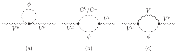
Figure 1: Relevant Feynman diagrams with scalars in the loop that have been considered to compute the oblique corrections. Here $\phi\in(\tilde{h},\tilde{s})$ when one-loop correction in the full theory is computed.

Equation (5) clearly shows that the light (heavy) scalar couplings to the SM particles are suppressed by a factor of $\cos\theta$ ($\sin\theta$). Therefore, the contributions to the gauge boson self-energies get modified by a factor of $\cos^{2}{\theta}$ or $\sin^{2}\theta$ depending on the neutral scalar coupled to. We then express the mixing angle regarding the BSM parameters in the potential. Limits are then imposed on the independent BSM parameters (in our case, it is just $\eta_{S}$) and the mass of the heavy scalar ($M_{\cal{S}}$) using the constraints of GFitter data Haller:2018nnx as shown in Fig. 2.

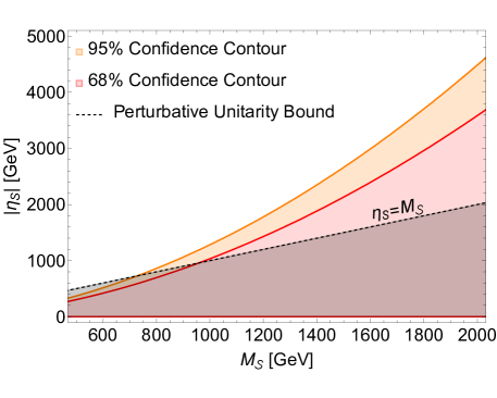
Figure 2: $95\%$ and $68\%$ confidence interval bounds on the BSM trilinear coupling $\eta_{S}$ and the Mass of the heavy scalar ($M_{\cal{S}}$) obtained from the full-theory calculation setting constraints from GFitter Haller:2018nnx . An additional unitarity bound is imposed which sets the limit of $\eta_{S}$, as $|\eta_{S}|\lesssim M_{\cal{S}}$ (see appendix B).

2.2 Real Singlet Model from SMEFT perspective

To investigate how well the effective theory replicates the minute signatures of the singlet extension of the SM described in Sec. 2.1 or, in turn, adjudge the significance of the higher-order effective corrections, we extend the effective series with relevant operator structures till dimension eight:

$${\cal{L}}={\cal{L}}_{\text{SM}}+\sum_{i}\frac{{\cal{C}}_{i}^{(6)}}{\Lambda^{2}}\,{\cal{O}}_{i}^{(6)}+\sum_{j}\frac{{\cal{C}}_{j}^{(8)}}{\Lambda^{4}}\,{\cal{O}}_{j}^{(8)}.$$ (8)

Here, the Wilson coefficients $\mathcal{C}_{i}$ parametrize the strengths of the operators $\mathcal{O}_{i}$ that are produced after integrating out the heavy real singlet scalar (for a complete matching of such operators at dimension six, see Refs. Banerjee:2022thk ). We have chosen the cut-off scale $\Lambda$ to be $m_{s}=M_{S}$. To validate EFT, as we will be working with small mixing, thus the parameter space of our interest will satisfy the following equivalence $M_{S}\simeq m_{s}$.

Figure 3: Tree-level correction to the gauge boson propagators due to the presence of effective operators.

In particular, this implies that in the case of effective theory, there may be tree-level electroweak corrections, as shown in Fig. 3, to Eq. (1) from the effective operators that may emerge in the process of integrating out heavy fields from the UV diagram and(or) through the renormalization group running of effective operators generated by integrating out tree-level heavy propagator at the cut-off scale. These contributions depend on the renormalization scale and play an essential role in our further computation, see also Jiang:2018pbd . Depending on whether the operators that could contribute to the dominant (when considered in a model-independent way) tree-level correction, as shown in Fig. 3, are generated at one-loop itself, the contributions from the operators generated at the tree level, which can modify the interactions at the one-loop, can become significant.

We categorically list the effective corrections to $\widehat{S},\widehat{T}$ up to one loop:

• Tree-level correction: Expanding the Lagrangian with dimension six and dimension eight operators can induce corrections to the transverse tree-level vector boson propagators ($\Pi_{VV^{\prime}}$) itself, which in turn modifies $\widehat{S}$, $\widehat{T}$ parameters Murphy:2020rsh

  $$\begin{split}\widehat{S}_{\text{eft,tree}}&=\frac{4\,c_{W}\,s_{W}\,v^{2}}{\alpha}\,\mathcal{C}_{HWB}^{(6)}\,+\frac{2\,c_{W}\,s_{W}\,v^{4}}{\alpha}\,\mathcal{C}_{HWB}^{(8)},\\ \widehat{T}_{\text{eft,tree}}&=-\frac{v^{2}}{2\,\alpha}\,\mathcal{C}_{H\mathcal{D}}^{(6)}\,-\,\frac{v^{4}}{2\,\alpha}\,\mathcal{C}_{H\mathcal{D},2}^{(8)}.\end{split}$$ (9)

  The expressions for modifying the individual $\Pi_{VV^{\prime}}$ functions are given in the appendix A.2. The dimension six operators contributing to Eq. (9) are generated at one-loop while integrating out the heavy field. The matching expressions for these coefficients are given in Tab. 1. We have also computed the one-loop matching for the dimension eight operators involved in Eq. (9) and noticed that these do not receive any correction while integrating out complete heavy loop diagrams. On the other hand, these coefficients receive contributions from removing the redundant structures at dimension six, as discussed in Ref. Banerjee:2022thk . Since the latter corresponds to a two-loop suppressed sub-leading contribution, we neglect the associated effects in our analysis.

  Operator	Op. Structure	Wilson coeffs.
  $\mathcal{O}_{H\square}^{(6)}$	$(H^{\dagger}H)\square(H^{\dagger}H)$	$-\frac{\eta_{\mathcal{S}}^{2}}{2\,M_{\mathcal{S}}^{4}}$
  ${\color[rgb]{0,0,1}\mathcal{O}_{HWB}^{(6)}}$	${\color[rgb]{0,0,1}(H^{\dagger}\tau^{I}H)W^{I}_{\mu\nu}B^{\mu\nu}}$	${\color[rgb]{0,0,1}\frac{g_{{}_{W}}g_{Y}\eta_{\mathcal{S}}^{2}}{128\,M_{\mathcal{S}}^{4}\,\pi^{2}}}$
  ${\color[rgb]{0,0,1}\mathcal{O}_{HD}^{(6)}}$	${\color[rgb]{0,0,1}(H^{\dagger}\mathcal{D}_{\mu}H)^{*}(H^{\dagger}\mathcal{D}^{\mu}H)}$	${\color[rgb]{0,0,1}-\frac{7g_{Y}^{2}\eta_{\mathcal{S}}^{2}}{288\,M_{\mathcal{S}}^{4}\,\pi^{2}}}$

  Table 1: Relevant operators that produce tree and one-loop corrections to the gauge boson self-energy. The structures in blue first appear at tree-level correction, whereas the rest of the operators contribute at one-loop first.

• One-loop insertion of operators: One-loop corrections to the oblique parameters are essential for the tree-level generated operators, for they provide a similar contribution as the operators that are produced at one-loop contributing to the tree-level propagator corrections shown in Eq. (9) for a model-dependent analysis. In our case, such a contribution arises from the operators $\mathcal{O}_{H\square}^{(6)}$ and $\mathcal{O}_{H\mathcal{D},1}^{(8)}$. The explicit forms of their structures are given in Tabs. 1 and 2, respectively. These operators modify the canonical form of the kinetic term for the Higgs field

  $$\mathcal{L}_{h,\text{kin}} = \frac{1}{2}\,\left(1-2\,v^{2}\mathcal{C}_{H\square}^{(6)}+\frac{v^{4}}{4}\mathcal{C}_{H\mathcal{D},1}^{(8)}\right)(\partial_{\mu}h)^{2},$$ (10)

  which can be removed by redefining the field $h^{\prime}\to Z_{h}\,h$ with

  $$Z_{h}=\left(1-v^{2}\,\mathcal{C}_{H\square}^{(6)}+\frac{v^{4}}{8}\,\mathcal{C}_{H\mathcal{D},1}^{(8)}\right).$$ (11)

  This implies that while computing the higher order corrections for EFT, we need to recall that $\phi=h^{\prime}\to Z_{h}\,h$ in Fig. 1. This also accounts for suitable modifications in the vertices, involving Higgs and Goldstone in Fig. 1. This correction, up to $\mathcal{O}(1/\Lambda^{4})$ capturing the effects from both $(\text{dimension six})^{2}$ and dimension eight terms, is incorporated by replacing the $\cos^{2}{\theta}$ with $Z_{h}^{2}$ and setting $\sin^{2}\theta$ to zero in the expressions shown in appendix A.1.

• RGE improved correction: It is important to include the running effects to the Wilson coefficients which arise at tree-level. $\widehat{T}_{\text{eft,tree}}$ in Eq. (9) at dimension six receives such an additional contribution from the operator $\mathcal{O}_{H\mathcal{D}}^{(6)}$. Contributions arising from the running of the coefficient of the operator $\mathcal{O}_{H\square}^{(6)}$ Jenkins:2013zja ; Alonso:2013hga

  $$16\pi^{2}\,\frac{d\,\mathcal{C}^{(6)}_{H\mathcal{D}}\,(\mu)}{d\ln{\mu}} = \frac{20}{3}\,g_{Y}^{2}\,\mathcal{C}_{H\square}^{(6)},$$

  $$\Longrightarrow\,\mathcal{C}_{H\mathcal{D}}^{(6)}\,|_{\text{RGE}} = -\frac{5\,g_{Y}^{2}\eta_{\mathcal{S}}^{2}}{24\,\pi^{2}\,M_{\mathcal{S}}^{4}}\,\log{\left[\frac{M_{Z}}{M_{\mathcal{S}}}\right]}.$$ (12)

  So the total contribution to $\mathcal{C}_{H\mathcal{D}}$ at the EW scale is:

  $$\mathcal{C}_{H\mathcal{D}}^{(6)}(M_{Z})={-\frac{7g_{Y}^{2}\eta_{\mathcal{S}}^{2}}{288\,M_{\mathcal{S}}^{4}\,\pi^{2}}}-\frac{5\,g_{Y}^{2}\eta_{\mathcal{S}}^{2}}{24\,\pi^{2}\,M_{\mathcal{S}}^{4}}\,\log{\left[\frac{M_{Z}}{M_{\mathcal{S}}}\right]}.$$ (13)

  The part of the beta function (cf. Eq. (• ‣ 2.2)) for the dimension eight Wilson coefficient $\mathcal{C}_{H\mathcal{D},2}^{(8)}$ and $\mathcal{C}_{HWB}^{(8)}$ stems from

  $$16\pi^{2}\,\frac{d\,\mathcal{C}_{H\mathcal{D},2}^{(8)}\,(\mu)}{d\ln{\mu}} = \frac{40}{3}\,g_{Y}^{2}\,(\mathcal{C}_{H\square}^{(6)})^{2}\,+\cfrac{10}{3}g_{Y}^{2}\mathcal{C}_{H\mathcal{D},1}^{(8)}\,+\mathcal{C}_{H^{4}D^{4},3}^{(8)}\left(-\cfrac{11}{24}g_{Y}^{4}-\cfrac{79}{48}g_{Y}^{2}g_{W}^{2}+3g_{Y}^{2}\lambda_{h}\right)$$

  $$\Longrightarrow\,\mathcal{C}_{H\mathcal{D},2}^{(8)}\,|_{\text{RGE}} = \cfrac{1}{16\pi^{2}}\Bigg{[}\frac{10\,g_{Y}^{2}\eta_{\mathcal{S}}^{4}}{3\,M_{\mathcal{S}}^{8}}+\cfrac{10}{3}g_{Y}^{2}\left(\frac{4\eta_{\mathcal{S}}^{2}k_{\mathcal{S}}}{M_{\mathcal{S}}^{6}}-\frac{8\lambda_{\mathcal{S}}\eta_{\mathcal{S}}^{2}k_{\mathcal{S}}}{M_{\mathcal{S}}^{6}}\right)$$ (14)

  $$+\cfrac{2\eta_{\mathcal{S}}^{2}}{M_{\mathcal{S}}^{6}}\left(-\cfrac{11}{24}g_{Y}^{4}-\cfrac{79}{48}g_{Y}^{2}g_{W}^{2}+3g_{Y}^{2}\lambda_{h}\right)\Bigg{]}\log{\left[\frac{M_{Z}}{M_{\mathcal{S}}}\right]},$$

  $$16\pi^{2}\,\frac{d\,\mathcal{C}_{HWB}^{(8)}\,(\mu)}{d\ln{\mu}} = \mathcal{C}_{H^{4}D^{4},3}^{(8)}\left(-\cfrac{11}{48}g_{Y}^{3}g_{W}-\cfrac{29}{24}g_{Y}g_{W}^{3}+g_{Y}g_{W}\lambda_{h}\right)$$

  $$\Longrightarrow\,\mathcal{C}_{HWB}^{(8)}\,|_{\text{RGE}} = \cfrac{\eta_{\mathcal{S}}^{2}}{8\pi^{2}M_{\mathcal{S}}^{6}}\left(-\cfrac{11}{48}g_{Y}^{3}g_{W}-\cfrac{29}{24}g_{Y}g_{W}^{3}+g_{Y}g_{W}\lambda_{h}\right)\log{\left[\frac{M_{Z}}{M_{\mathcal{S}}}\right]},$$ (15)

with $g_{Y}=e/c_{W},g_{W}=e/s_{W}$. In addition to contributions from dimension six effective operators, we also compute the contribution to dimension eight operators from the equations of motion of the dimension six operators and the RGE-improved corrections due to dimension six operators, see further Refs. Li:2020gnx ; Murphy:2020rsh ; Chala:2021pll ; DasBakshi:2022mwk . We note that the correction to $\Delta\widehat{T}$ and $\Delta\widehat{S}$ due to the dimension eight inclusion is of the order of the deviations. Thus, dimension eight interactions may be crucial to bringing EFT predictions close to the full theory for given measured constraints.

3 Full theory vs EFT

In this section, we compare a full theory and its effective version captured in SMEFT. We carefully investigate how the inclusion of higher mass dimensional operators, suppressed by the mass of the heavy integrated-out field, in the EFT expansion affects the computation of our chosen observable $(\widehat{T},\widehat{S})$. For this, we categorize the EFT contribution into three parts. To start with, we discuss the dimension six $(d_{6})$ part, which contributes at ${\mathcal{O}}(M_{\mathcal{S}}^{-2})$ containing linear dimension six Wilson coefficients (WCs). Here, we include the cumulative effects of field redefinition and radiative corrections on the oblique parameters. Then, we consider the corrections from the dimension eight $(d_{8})$ operators that are linear functions of dimension eight WCs at the ${\mathcal{O}}(M_{\mathcal{S}}^{-4})$. We also include the dimension eight equivalent contributions (referred to as $(d_{6})^{2}$), at ${\mathcal{O}}(M_{\mathcal{S}}^{-4})$, from dimension six operators which are quadratic functions of dimension six WCs. This takes care of the radiative generation of dimension eight operators from dimension six ones, see Eq. (• ‣ 2.2) and the expansion of $Z_{h}^{2}$. We list all those operators that contribute in different orders:

• $d_{6}$:  $\mathcal{C}_{HD}^{(6)},\;\mathcal{C}_{HWB}^{(6)},\;\mathcal{C}_{H\square}^{(6)}$ ;

• $d_{8}$:  $\mathcal{C}_{H\mathcal{D},1}^{(8)},\;\mathcal{C}_{H\mathcal{D},2}^{(8)},\;\mathcal{C}_{H^{4}D^{4},3}^{(8)},\;\mathcal{C}_{HWB}^{(8)}$ ;

• $(d_{6})^{2}:$ $(\mathcal{C}_{H\square}^{(6)})^{2}$  .

Operator	Op. Structure	Wilson coeffs.
$\mathcal{O}_{HD,1}^{(8)}$	$(H^{\dagger}H)^{2}\,(\mathcal{D}_{\mu}H^{\dagger}\mathcal{D}_{\mu}H)$	$\frac{4\eta_{\mathcal{S}}^{2}k_{\mathcal{S}}}{M_{\mathcal{S}}^{6}}-\frac{8\lambda_{\mathcal{S}}\eta_{\mathcal{S}}^{2}k_{\mathcal{S}}}{M_{\mathcal{S}}^{6}}$
$\mathcal{O}_{H^{4}D^{4},3}^{(8)}$	$(\mathcal{D}_{\mu}H^{\dagger}\mathcal{D}^{\mu}H)(\mathcal{D}_{\nu}H^{\dagger}\mathcal{D}^{\nu}H)$	$\frac{2\eta_{\mathcal{S}}^{2}}{M_{\mathcal{S}}^{6}}$

Table 2: Relevant operators that produce tree and one-loop corrections to the gauge boson self-energy. The structures in blue first appear at tree-level correction, whereas the rest of the operators contribute at one-loop first.

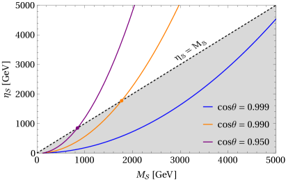
(a)

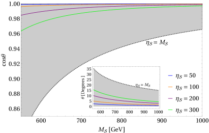
(b)

Figure 4: (a) shows the variation of the trilinear coupling with respect to heavy scalar mass. The orange and yellow dots denote $\eta_{\mathcal{S}}$ values to reproduce values of the respective $\cos^{2}\theta$ choices. In (b) we show how the mixing angle is a function of the heavy mass for fixed values of the trilinear coupling $\eta_{\mathcal{S}}$. In both plots, the gray-shaded region respects perturbative unitarity (see appendix B). We can give two plots separately. The first one shows how large cos theta can be achieved for wide ranges of m. The second one is the allowed range of theta that can be achieved by minimizing $\eta_{S}$.

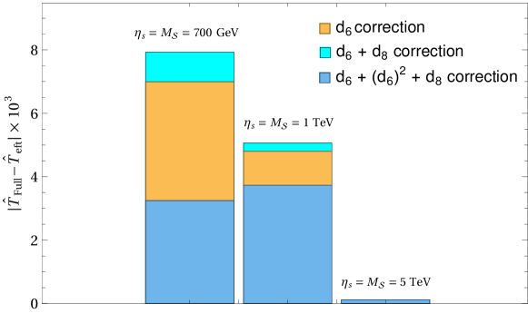
Figure 5: Impact of individual contributions on $\Delta\widehat{T}=|\widehat{T}_{\text{Full}}-\widehat{T}_{\text{eft}}|$ for three benchmark choices of $\eta_{s}=M_{S}$, having maximal allowed mixing. $\Delta\widehat{T}$, computed upto $\mathcal{O}(M_{S}^{-2})$, i.e., truncating effective Lagrangian at mass dimension six, receives a positive contribution from dimension eight operators. Though, the total contributions upto order $\mathcal{O}(M_{S}^{-2})$ reduces $\Delta\widehat{T}$ signifying inclusion of dimension eight operators brings the effective theory prediction relatively closer to that from the full theory.

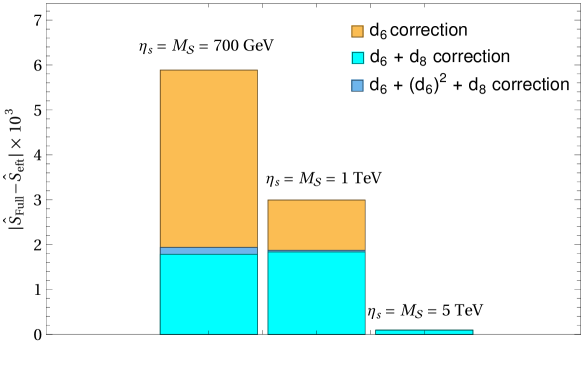
Figure 6: Impact of individual contributions on $\Delta\widehat{S}=|\widehat{S}_{\text{Full}}-\widehat{S}_{\text{eft}}|$ for three benchmark choices of $\eta_{s}=M_{S}$. We note that adding the RG evolution contribution from dimension eight operators improves the effective theory to replicate the full theory.

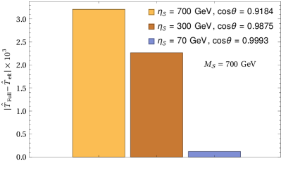
(a)  

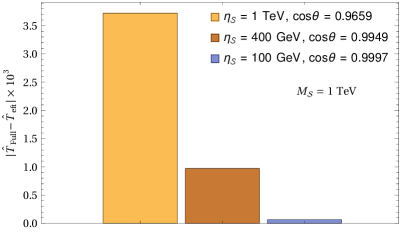
(b)  

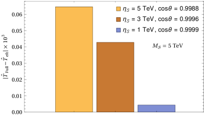
(c)  

Figure 7: Difference between full theory and the EFT computation for $\widehat{T}$ parameter at different heavy field mass scales. The mass scales are chosen to be (a) 700 GeV, (b) 1 TeV and (c) 5 TeV. The values for $\eta_{S}$ are chosen such that they satisfy the unitarity bounds.

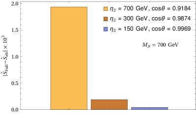
(a)  

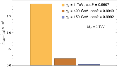
(b)  

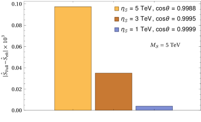
(c)  

Figure 8: Difference between full theory and the EFT computation for $\widehat{S}$ parameter at different heavy field mass scales. The mass scales are chosen to be (a) 700 GeV, (b) 1 TeV and (c) 5 TeV. The values for $\eta_{S}$ are chosen such that they satisfy the unitarity bounds.

We investigate the departure of the truncated-EFT computation at dimension six from the full theory calculations and the role that the Higgs mixing plays in matching these two. The mixing can be expressed as a function of the trilinear coupling $\eta_{S}$ and the heavy cut-off scale $M_{\mathcal{S}}$, for allowed $\eta_{S}$ values, the decoupling can be quantified through the difference of the two theories. In Fig. 4(a), we show the lines for the constant mixing angles that allow a single $\eta_{S}$ value for each choice of the cut-off. We also impose the constraint from the perturbative unitarity that rules out a specific region in the $\eta_{S}-M_{\mathcal{S}}$ plane, in turn putting a lower-bound for the mixing for each value of the cut-off $M_{\mathcal{S}}$, that can be seen in Fig. 4(b).

Intuitively, adding higher and higher order terms in EFT expansion would take the EFT closer to the full theory. This concept is illustrated through the $\widehat{T}$ parameter in Fig. 5. Here, we consider three different types of contributions. Firstly, the leading order terms in the expansion, i.e., $d_{6}$ ones. Then, we add $d_{8}$ contributions and finally, the $(d_{6})^{2}$ ones. In passing, we want to highlight that though the $d_{8}$ term adds positively to the difference between the full theory and EFT, the further addition of $(d_{6})^{2}$, the equivalent of $d_{8}$ ones, allows us to capture the complete contribution at $\mathcal{O}(M_{\mathcal{S}}^{-4})$. Ultimately, it reflects that going to higher order in EFT expansion reduces the gap between full theory and EFT, especially for a relatively large mixing. We perform similar analyses for $\widehat{S}$ parameter in Fig. 6. We draw a similar conclusion as the previous one, and that makes our conclusion more generic.

In Fig. 7, we have calculated the difference between full theory and EFT in calculating the $\widehat{T}$ parameter for three different heavy mass scales. In each subfigure, we have shown that if we lower the value of $\eta_{S}$ for a fixed mass, the value of $\cos\theta$ increases. As the $\cos\theta$ reaches unity, the full theory and EFT are in excellent agreement, which is expected as the new physics contribution vanishes. It is also evident that for a fixed $\eta_{S}$, once we go for higher masses the difference also decreases. This illustrates the interplay among the coupling $\eta_{S}$, the heavy mass scale $M_{\mathcal{S}}$, and mixing parameter $\cos\theta$. One can tune the value of these parameters so that EFT can be a good explanation for the full theory. Doing the same kind of investigation for the $\widehat{S}$ parameter in Fig. 8 further emphasises the idea.

4 Summary and Conclusions

Effective Field Theory is a powerful tool to look for deviations from the SM expectation in a theoretically well-motivated way. In a modern sense, it enables us to extend good quantum field theoretic properties to generic departures from the SM interactions, with potential relevance for UV complete scenarios depending on the accuracy with which constraints can be formulated. Along these lines, a set of particularly well-motivated observables are the oblique corrections as a subset of relevant electroweak corrections. In this work, we have analysed these observables from their dimension six and eight points of view with a critical perspective on how accurately EFT methods describe the full theory in the singlet extension scenarios where decoupling and alignment limits are exceptionally transparent. As expected, EFT approximates the full theory well in regions where it is valid. However, moving away from the alignment/decoupling limit, the relevance of the higher-dimensional terms in the EFT expansion quickly becomes relevant. Although these ranges are currently not probed by the experiments, it demonstrates the need to include higher-dimensional corrections (chiefly squared dimension six terms) to well-approximate the full theory. Furthermore, as Higgs boson mixing is a feature in almost all BSM theories with a non-minimal Higgs sector, this shows the necessity to go beyond dimension six interactions when data is very precise or when we want to inform a potential UV scenario accurately.

Appendix A Gauge boson two-point functions

A.1 Modification due to a singlet scalar extension

We note down the modifications to the gauge boson two-point functions due to the presence of a new heavier scalar degree of freedom. Here, only the contributions from the scalar-involved diagrams are presented. The BSM contribution to the two-point functions (in Feynman gauge) are then Hahn:2000kx

$$\Pi_{ZZ}(p^{2}) = \left[-\frac{M_{W}^{4}B_{0}\left(p^{2},M_{h}^{2},M_{Z}^{2}\right)}{4\pi^{2}c_{W}^{4}v^{2}}+\frac{M_{W}^{2}B_{00}\left(p^{2},M_{h}^{2},M_{Z}^{2}\right)}{4\pi^{2}c_{W}^{2}v^{2}}-\frac{M_{h}^{2}M_{W}^{2}\left(1-\log\left(\frac{M_{h}^{2}}{\mu^{2}}\right)\right)}{16\pi^{2}c_{W}^{2}v^{2}}\right]$$ (16)

$$\cos^{2}{\theta}+\left[-\frac{M_{W}^{4}B_{0}\left(p^{2},M_{\cal{S}}^{2},M_{Z}^{2}\right)}{4\pi^{2}c_{W}^{4}v^{2}}+\frac{M_{W}^{2}B_{00}\left(p^{2},M_{\cal{S}}^{2},M_{Z}^{2}\right)}{4\pi^{2}c_{W}^{2}v^{2}}\right.$$

$$\left.-\frac{M_{\cal{S}}^{2}M_{W}^{2}\left(1-\log\left(\frac{M_{\cal{S}}^{2}}{\mu^{2}}\right)\right)}{16\pi^{2}c_{W}^{2}v^{2}}\right]\sin^{2}{\theta},$$

$$\Pi_{WW}(p^{2}) = \left[-\frac{M_{W}^{4}B_{0}\left(p^{2},M_{h}^{2},M_{W}^{2}\right)}{4\pi^{2}v^{2}}+\frac{M_{W}^{2}B_{00}\left(p^{2},M_{h}^{2},M_{W}^{2}\right)}{4\pi^{2}v^{2}}-\frac{M_{h}^{2}M_{W}^{2}\left(1-\log\left(\frac{M_{h}^{2}}{\mu^{2}}\right)\right)}{16\pi^{2}v^{2}}\right]$$ (17)

$$\cos^{2}{\theta}+\left[-\frac{M_{W}^{4}B_{0}\left(p^{2},M_{\cal{S}}^{2},M_{W}^{2}\right)}{4\pi^{2}v^{2}}+\frac{M_{W}^{2}B_{00}\left(p^{2},M_{\cal{S}}^{2},M_{W}^{2}\right)}{4\pi^{2}v^{2}}\right.$$

$$-\left.\frac{M_{\cal{S}}^{2}M_{W}^{2}\left(1-\log\left(\frac{M_{\cal{S}}^{2}}{\mu^{2}}\right)\right)}{16\pi^{2}v^{2}}\right]\sin^{2}{\theta},$$

$$\Pi_{\gamma\gamma}(p^{2}) = \Pi_{\gamma Z}(p^{2})=0\,,$$ (18)

where, the Passarino-Veltman functions Passarino:1978jh (see also Denner:1991kt ; Denner:2019vbn ) $A_{0}$, $B_{0}$ and $B_{00}$ capture the scalar one-loop dynamics (the vev is fixed via $v=2M_{W}s_{W}/e$). We have cross checked these results numerically against previous results Bowen:2007ia ; Englert:2011yb .

A.2 Modification due to the corresponding EFT at tree-level

We note down the tree-level correction to the gauge boson propagators as shown in Fig. 3 due to the presence of effective operators.

$$\Pi_{WW}^{(\text{EFT})}(p^{2}) = \frac{g_{W}^{2}\,v^{6}}{16}\mathcal{C}_{H\mathcal{D},1}^{(8)}-\frac{g_{W}^{2}\,v^{6}}{16}\mathcal{C}_{H\mathcal{D},2}^{(8)}+p^{2}v^{4}\,\mathcal{C}_{HW}^{(8)}+2p^{2}v^{2}\mathcal{C}_{HW}^{(6)},$$ (19)

$$\Pi_{ZZ}^{(\text{EFT})}(p^{2}) = \frac{c_{W}^{2}g_{W}^{2}v^{6}}{16}\mathcal{C}_{H\mathcal{D},1}^{(8)}+\frac{c_{W}^{2}g_{W}^{2}v^{6}}{16}\mathcal{C}_{H\mathcal{D},2}^{(8)}+\frac{c_{W}^{2}g_{W}^{2}v^{4}}{8}\mathcal{C}_{H\mathcal{D}}^{(6)}+c_{W}^{2}p^{2}v^{4}\mathcal{C}_{HW}^{(8)}$$ (20)

$$+2c_{W}^{2}p^{2}v^{2}\mathcal{C}_{HW}^{(6)}+\frac{c_{W}s_{W}g_{W}g_{Y}v^{6}}{8}\mathcal{C}_{H\mathcal{D},1}^{(8)}+\frac{c_{W}s_{W}g_{W}g_{Y}v^{6}}{8}\mathcal{C}_{H\mathcal{D},2}^{(8)}$$

$$+\frac{c_{W}s_{W}g_{W}g_{Y}v^{4}}{4}\mathcal{C}_{H\mathcal{D}}^{(6)}+p^{2}c_{W}s_{W}v^{4}\,\mathcal{C}_{HWB}^{(8)}+2p^{2}c_{W}s_{W}v^{2}\mathcal{C}_{{HWB}}^{(6)}$$

$$+\frac{s_{W}^{2}g_{Y}^{2}v^{6}\mathcal{C}_{H\mathcal{D},1}^{(8)}}{16}+\frac{s_{W}^{2}g_{Y}^{2}v^{6}\mathcal{C}_{H\mathcal{D},2}^{(8)}}{16}+\frac{s_{W}^{2}g_{Y}^{2}v^{4}\mathcal{C}_{H\mathcal{D}}^{(6)}}{8}$$

$$+p^{2}s_{W}^{2}v^{4}\mathcal{C}_{HB}^{(8)}+2p^{2}s_{W}^{2}v^{2}\mathcal{C}_{{HB}}^{(6)},$$

$$\Pi_{\gamma\gamma}^{(\text{EFT})}(p^{2}) = \frac{c_{W}^{2}g_{Y}^{2}v^{6}}{16}\mathcal{C}_{H\mathcal{D},1}^{(8)}+\frac{c_{W}^{2}g_{Y}^{2}v^{6}}{16}\mathcal{C}_{H\mathcal{D},2}^{(8)}+\frac{c_{W}^{2}g_{Y}^{2}v^{4}}{8}\mathcal{C}_{H\mathcal{D}}^{(6)}+p^{2}c_{W}^{2}v^{4}\mathcal{C}_{HB}^{(8)}$$ (21)

$$+2p^{2}c_{W}^{2}v^{2}\mathcal{C}_{{HB}}^{(6)}-\frac{c_{W}s_{W}g_{W}g_{Y}v^{6}}{8}\mathcal{C}_{H\mathcal{D},1}^{(8)}-\frac{c_{W}s_{W}g_{W}g_{Y}v^{6}}{8}\mathcal{C}_{H\mathcal{D},2}^{(8)}$$

$$-\frac{g_{W}g_{Y}c_{W}s_{W}v^{4}}{4}\mathcal{C}_{H\mathcal{D}}^{(6)}-p^{2}c_{W}s_{W}v^{4}\mathcal{C}_{HWB}^{(8)}-2p^{2}c_{W}s_{W}v^{2}\mathcal{C}_{HWB}^{(6)}$$

$$+\frac{s_{W}^{2}g_{W}^{2}v^{6}}{16}\mathcal{C}_{H\mathcal{D},1}^{(8)}+\frac{s_{W}^{2}g_{W}^{2}v^{6}}{16}\mathcal{C}_{H\mathcal{D},2}^{(8)}+\frac{s_{W}^{2}g_{W}^{2}v^{6}}{8}\mathcal{C}_{H\mathcal{D}}^{(6)}$$

$$+p^{2}s_{W}^{2}v^{4}\mathcal{C}_{HW}^{(8)}+2p^{2}s_{W}^{2}v^{2}\mathcal{C}_{HW}^{(6)},$$

$$\Pi_{\gamma Z}^{(\text{EFT})}(p^{2}) = -\frac{c_{W}^{2}g_{W}g_{Y}v^{6}}{16}\mathcal{C}_{H\mathcal{D},1}^{(8)}-\frac{c_{W}^{2}g_{W}g_{Y}v^{6}}{16}\mathcal{C}_{H\mathcal{D},2}^{(8)}-\frac{c_{W}^{2}g_{W}g_{Y}v^{4}}{8}\mathcal{C}_{H\mathcal{D}}^{(6)}$$ (22)

$$-\frac{p^{2}c_{W}^{2}v^{4}}{2}\mathcal{C}_{HWB}^{(8)}-p^{2}c_{W}^{2}v^{2}\mathcal{C}_{{HWB}}^{(6)}+\frac{c_{W}s_{W}g_{W}^{2}v^{6}}{16}\mathcal{C}_{H\mathcal{D},1}^{(8)}+\frac{c_{W}s_{W}g_{W}^{2}v^{6}}{16}\mathcal{C}_{H\mathcal{D},2}^{(8)}$$

$$+\frac{c_{W}s_{W}g_{W}^{2}v^{4}}{8}\mathcal{C}_{H\mathcal{D}}^{(6)}-\frac{c_{W}s_{W}g_{Y}^{2}v^{6}}{16}\mathcal{C}_{H\mathcal{D},1}^{(8)}-\frac{c_{W}s_{W}g_{Y}^{2}v^{6}}{16}\mathcal{C}_{H\mathcal{D},2}^{(8)}$$

$$-\frac{c_{W}s_{W}g_{Y}^{2}v^{4}}{8}\mathcal{C}_{H\mathcal{D}}^{(6)}-p^{2}c_{W}s_{W}v^{4}\mathcal{C}_{HB}^{(8)}+p^{2}c_{W}s_{W}v^{4}\mathcal{C}_{HW}^{(8)}-2p^{2}c_{W}s_{W}v^{2}C_{HB}^{(6)}$$

$$+2p^{2}c_{W}s_{W}v^{2}\mathcal{C}_{HW}^{(6)}+\frac{s_{W}^{2}g_{W}g_{Y}v^{6}}{16}\mathcal{C}_{H\mathcal{D},1}^{(8)}+\frac{s_{W}^{2}g_{W}g_{Y}v^{6}}{16}\mathcal{C}_{H\mathcal{D},2}^{(8)}+\frac{s_{W}^{2}g_{W}g_{Y}v^{4}}{8}\mathcal{C}_{H\mathcal{D}}^{(6)}$$

$$+\frac{p^{2}s_{W}v^{4}}{2}\mathcal{C}_{HWB}^{(8)}+p^{2}s_{W}^{2}v^{2}\mathcal{C}_{HWB}^{(6)}.$$

The couplings are given by $g_{W}=e/s_{W},g_{Y}=e/c_{W}$.

Appendix B Unitarity Constraints

Unitarity provides a suitable tool to gauge whether the matching is indeed for perturbative choices of the UV model parameters. Perturbativity, in one way or another, is implicitly assumed in analysing any collider data and this extends to the electroweak precision constraints as well. To this end, we consider the partial wave constraints that can be derived from longitudinal gauge boson scattering to identify the regions of validity this way. The zeroth partial wave relevant for this is given for scattering $i_{1}\,i_{2}\to f_{1}\,f_{2}$ (see Ref. Jacob:1959at )

$$a_{fi}^{0}=\frac{\beta^{1/4}(s,m_{i,1}^{2},m_{i,1}^{2})\,\beta^{1/4}(s,m_{f,1}^{2},m_{f,1}^{2})}{32\pi s}\int_{-1}^{1}\text{d}\cos\theta\,\,{\cal{M}}(\sqrt{s},\cos\theta)\,,$$ (23)

suppressing factors of $1/\sqrt{2}$ for identical particles in the initial $i$ or final state $f$. $\sqrt{s}$ denotes the centre-of-mass energy, and $\theta$ is the scattering angle in this frame for the $2\to 2$ scattering process described by the amplitude $\sim{\cal{M}}$. Furthermore,

$$\beta(x,y,z)=x^{2}+y^{2}+z^{2}-2xy-2yz-2xz\,.$$ (24)

such that $\lim_{s\to\infty}\beta^{2}/s=1$. Unitarity of the $S$ matrix then translates for $f=i$ to the conditions

$$|\text{Re}\,a_{ii}^{0}|\leq\frac{1}{2}\quad\hbox{and}\quad|\text{Im}\,a_{ii}^{0}|\leq 1\,.$$ (25)

of which we use the first one to obtain the constraints in Sec. 2. The presence of large $\eta_{S}\sim M_{\cal{S}}$ leads to unitarity violation through ${\cal{S}}$ contributions to $hh\to hh$ via the $s,t,u$ channels as well as large values of $M_{\cal{S}}$ for $\cos^{2}\theta\neq 1$ in longitudinal gauge boson scattering Lee:1977eg . Numerical investigation shows that for our choice close to the alignment limits longitudinal unitarity constraints are not as relevant as $hh$ scattering constraints. Assuming perturbative unitarity up to a cut-off scale $\sim M_{\cal{S}}$ requires $\eta_{S}\lesssim M_{\cal{S}}$. This reflects the fact that when a dimensionful coupling (i.e. a mass scale) such as $\eta_{S}$ becomes comparable to a UV cut-off ($M_{\cal{S}}$ in the EFT description), we enter strong coupling. This is also visible from the expansion of phenomenologically relevant quantities such as Eq. (6), which scales $\sim v\eta_{S}/M_{\cal{S}}^{2}$ in the EFT regime $M_{\cal{S}}\gg M_{h}$.

References

- (1) S. Weinberg, Phenomenological Lagrangians, Physica A 96 (1979) 327–340.
- (2) B. Grzadkowski, M. Iskrzynski, M. Misiak and J. Rosiek, Dimension-Six Terms in the Standard Model Lagrangian, JHEP 10 (2010) 085, [1008.4884].
- (3) M. Jiang, N. Craig, Y.-Y. Li and D. Sutherland, Complete one-loop matching for a singlet scalar in the Standard Model EFT, JHEP 02 (2019) 031, [1811.08878].
- (4) U. Haisch, M. Ruhdorfer, E. Salvioni, E. Venturini and A. Weiler, Singlet night in Feynman-ville: one-loop matching of a real scalar, JHEP 04 (2020) 164, [2003.05936].
- (5) V. Gherardi, D. Marzocca and E. Venturini, Matching scalar leptoquarks to the SMEFT at one loop, JHEP 07 (2020) 225, [2003.12525].
- (6) Y. Du, X.-X. Li and J.-H. Yu, Neutrino seesaw models at one-loop matching: discrimination by effective operators, JHEP 09 (2022) 207, [2201.04646].
- (7) S. Dawson and C. W. Murphy, Standard Model EFT and Extended Scalar Sectors, Phys. Rev. D 96 (2017) 015041, [1704.07851].
- (8) D. Zhang and S. Zhou, Complete one-loop matching of the type-I seesaw model onto the Standard Model effective field theory, JHEP 09 (2021) 163, [2107.12133].
- (9) S. Dittmaier, S. Schuhmacher and M. Stahlhofen, Integrating out heavy fields in the path integral using the background-field method: general formalism, Eur. Phys. J. C 81 (2021) 826, [2102.12020].
- (10) X. Li, D. Zhang and S. Zhou, One-loop matching of the type-II seesaw model onto the Standard Model effective field theory, JHEP 04 (2022) 038, [2201.05082].
- (11) D. Zhang, Complete One-loop Structure of the Type-(I+II) Seesaw Effective Field Theory, 2208.07869.
- (12) A. Carmona, A. Lazopoulos, P. Olgoso and J. Santiago, Matchmakereft: automated tree-level and one-loop matching, SciPost Phys. 12 (2022) 198, [2112.10787].
- (13) T. Cohen, X. Lu and Z. Zhang, STrEAMlining EFT Matching, SciPost Phys. 10 (2021) 098, [2012.07851].
- (14) S. Das Bakshi, J. Chakrabortty and S. K. Patra, CoDEx: Wilson coefficient calculator connecting SMEFT to UV theory, Eur. Phys. J. C 79 (2019) 21, [1808.04403].
- (15) C. W. Murphy, Dimension-8 Operators in the Standard Model Effective Field Theory, 2005.00059.
- (16) H.-L. Li, Z. Ren, J. Shu, M.-L. Xiao, J.-H. Yu and Y.-H. Zheng, Complete set of dimension-eight operators in the standard model effective field theory, Phys. Rev. D 104 (2021) 015026, [2005.00008].
- (17) U. Banerjee, J. Chakrabortty, C. Englert, S. U. Rahaman and M. Spannowsky, Integrating out heavy scalars with modified EOMs: matching computation of dimension-eight SMEFT coefficients, 2210.14761.
- (18) S. Dawson, D. Fontes, S. Homiller and M. Sullivan, Role of dimension-eight operators in an EFT for the 2HDM, Phys. Rev. D 106 (2022) 055012, [2205.01561].
- (19) S. Dawson, P. P. Giardino and S. Homiller, Uncovering the High Scale Higgs Singlet Model, Phys. Rev. D 103 (2021) 075016, [2102.02823].
- (20) G. M. Pruna and T. Robens, Higgs singlet extension parameter space in the light of the LHC discovery, Phys. Rev. D 88 (2013) 115012, [1303.1150].
- (21) T. Binoth and J. J. van der Bij, Influence of strongly coupled, hidden scalars on Higgs signals, Z. Phys. C 75 (1997) 17–25, [hep-ph/9608245].
- (22) M. Bowen, Y. Cui and J. D. Wells, Narrow trans-TeV Higgs bosons and H — hh decays: Two LHC search paths for a hidden sector Higgs boson, JHEP 03 (2007) 036, [hep-ph/0701035].
- (23) C. Englert, T. Plehn, D. Zerwas and P. M. Zerwas, Exploring the Higgs portal, Phys. Lett. B 703 (2011) 298–305, [1106.3097].
- (24) B. Batell, S. Gori and L.-T. Wang, Exploring the Higgs Portal with 10/fb at the LHC, JHEP 06 (2012) 172, [1112.5180].
- (25) Anisha, S. Das Bakshi, S. Banerjee, A. Biekötter, J. Chakrabortty, S. Kumar Patra et al., Effective limits on single scalar extensions in the light of recent LHC data, 2111.05876.
- (26) M. E. Peskin and T. Takeuchi, Estimation of oblique electroweak corrections, Phys. Rev. D 46 (Jul, 1992) 381–409.
- (27) G. Altarelli and R. Barbieri, Vacuum polarization effects of new physics on electroweak processes, Physics Letters B 253 (1991) 161–167.
- (28) D. Y. Bardin, P. Christova, M. Jack, L. Kalinovskaya, A. Olchevski, S. Riemann et al., ZFITTER v.6.21: A Semianalytical program for fermion pair production in annihilation, Comput. Phys. Commun. 133 (2001) 229–395, [hep-ph/9908433].
- (29) H. Flacher, M. Goebel, J. Haller, A. Hocker, K. Monig and J. Stelzer, Revisiting the Global Electroweak Fit of the Standard Model and Beyond with Gfitter, Eur. Phys. J. C 60 (2009) 543–583, [0811.0009].
- (30) R. Barbieri, A. Pomarol, R. Rattazzi and A. Strumia, Electroweak symmetry breaking after LEP-1 and LEP-2, Nucl. Phys. B 703 (2004) 127–146, [hep-ph/0405040].
- (31) J. Haller, A. Hoecker, R. Kogler, K. Mönig, T. Peiffer and J. Stelzer, Update of the global electroweak fit and constraints on two-Higgs-doublet models, Eur. Phys. J. C 78 (2018) 675, [1803.01853].
- (32) E. E. Jenkins, A. V. Manohar and M. Trott, Renormalization Group Evolution of the Standard Model Dimension Six Operators I: Formalism and lambda Dependence, JHEP 10 (2013) 087, [1308.2627].
- (33) R. Alonso, E. E. Jenkins, A. V. Manohar and M. Trott, Renormalization Group Evolution of the Standard Model Dimension Six Operators III: Gauge Coupling Dependence and Phenomenology, JHEP 04 (2014) 159, [1312.2014].
- (34) M. Chala, G. Guedes, M. Ramos and J. Santiago, Towards the renormalisation of the Standard Model effective field theory to dimension eight: Bosonic interactions I, SciPost Phys. 11 (2021) 065, [2106.05291].
- (35) S. Das Bakshi, M. Chala, A. Díaz-Carmona and G. Guedes, Towards the renormalisation of the Standard Model effective field theory to dimension eight: bosonic interactions II, Eur. Phys. J. Plus 137 (2022) 973, [2205.03301].
- (36) T. Hahn, Generating Feynman diagrams and amplitudes with FeynArts 3, Comput. Phys. Commun. 140 (2001) 418–431, [hep-ph/0012260].
- (37) G. Passarino and M. J. G. Veltman, One Loop Corrections for e+ e- Annihilation Into mu+ mu- in the Weinberg Model, Nucl. Phys. B 160 (1979) 151–207.
- (38) A. Denner, Techniques for calculation of electroweak radiative corrections at the one loop level and results for W physics at LEP-200, Fortsch. Phys. 41 (1993) 307–420, [0709.1075].
- (39) A. Denner and S. Dittmaier, Electroweak Radiative Corrections for Collider Physics, Phys. Rept. 864 (2020) 1–163, [1912.06823].
- (40) M. Jacob and G. C. Wick, On the General Theory of Collisions for Particles with Spin, Annals Phys. 7 (1959) 404–428.
- (41) B. W. Lee, C. Quigg and H. B. Thacker, Weak Interactions at Very High-Energies: The Role of the Higgs Boson Mass, Phys. Rev. D 16 (1977) 1519.