Statistics of phase space localization measures and quantum chaos in the kicked top model

Abstract

Quantum chaos plays a significant role in understanding several important questions of recent theoretical and experimental studies. Here, by focusing on the localization properties of eigenstates in phase space (by means of Husimi functions), we explore the characterizations of quantum chaos using the statistics of the localization measures, that is the inverse participation ratio and the Wehrl entropy. We consider the paradigmatic kicked top model, which shows a transition to chaos with increasing the kicking strength. We demonstrate that the distributions of the localization measures exhibit a drastic change as the system undergoes the crossover from integrability to chaos. We also show how to identify the signatures of quantum chaos from the central moments of the distributions of localization measures. Moreover, we find that the localization measures in the fully chaotic regime apparently universally exhibit the beta distribution, in agreement with previous studies in the billiard systems and the Dicke model. Our results contribute to a further understanding of quantum chaos and shed light on the usefulness of the statistics of phase space localization measures in diagnosing the presence of quantum chaos, as well as the localization properties of eigenstates in quantum chaotic systems.

I Introduction

The importance of quantum chaos in understanding several fundamental questions that arise in recent experimental and theoretical works, has triggered a great deal of efforts in the study of quantum chaos in different areas of physics Haake (2010); Stöckmann (1999); Nandkishore and Huse (2015); D’Alessio et al. (2016); Borgonovi et al. (2016); Deutsch (2018); Maldacena et al. (2016); Kos et al. (2018); Jahnke (2019); Bertini et al. (2019); Lerose and Pappalardi (2020). In contrast to the case of classical chaos, which is well defined as the exponential divergence of the closest orbits for initial perturbations Lichtenberg and Lieberman (2013); Cvitanovic et al. (2005), the definition of quantum chaos in the narrow sense remains an open question Robnik (2020). One, therefore, turns to focus on how to probe and measure the signatures of chaos in various quantum systems Haake (2010); Stöckmann (1999); Bastarrachea-Magnani et al. (2016); Chan et al. (2018); Friedman et al. (2019); Mondal et al. (2020); Kobrin et al. (2021); Muñoz Arias et al. (2021); Pausch et al. (2021a); Fogarty et al. (2021). To date, the presence of chaos in a quantum system is commonly ascertained from its spectral properties. It is well known that the energy spectrum of quantum systems which are classically chaotic has universal statistical properties, which are consistent with the predictions of the random matrix theory (RMT) Casati et al. (1980); Mehta (2004); Bohigas et al. (1984); Berry (1985); Sieber and Richter (2001); Guhr et al. (1998); Müller et al. (2004). As a consequence, the RMT sets a benchmark to identify the emergence of chaos in quantum systems. According to RMT, for example, a quantum system is said to be a chaotic system when its level spacing distribution follows the universal GOE/GUE/GSE level statistics, well approximated by the celebrated Wigner surmise Mehta (2004); Wigner (1958), or its spectral form factor exhibits a robust linear ramp Haake (2010); Stöckmann (1999); Bertini et al. (2018); Liu (2018); Chen and Ludwig (2018); Flack et al. (2020); Braun et al. (2020); Khramtsov and Lanina (2021).

An alternative way to capture the onset of chaos in quantum systems is to investigate the structure of eigenstates. The structure of eigenstates in quantum chaotic systems is essential to understand the thermalization mechanism in isolated systems D’Alessio et al. (2016); Borgonovi et al. (2016); Deutsch (2018, 1991); Srednicki (1994); Rigol et al. (2008). For quantum chaotic systems, it has been demonstrated that the mid-spectrum eigenstates are well described by the eigenstates of random matrices taken from the Gaussian ensembles of RMT Borgonovi et al. (2016); Kus et al. (1988). The eigenstates of Gaussian ensembles are random vectors with components that are independent Gaussian random numbers. Although this feature of eigenstates has been used as a witness of quantum chaos, several remarkable exceptions in both single-particle Fishman et al. (1982); Heller (1984); Geisel et al. (1986); Casati et al. (1990); Bäcker et al. (1997) and many-body quantum chaotic systems Serbyn et al. (2021); Pilatowsky-Cameo et al. (2021); Chandran et al. (2023) imply that further analysis on the structure of eigenstates in quantum chaotic systems is still required.

The structure of eigenstates can be examined in various ways, such as the fractality of the eigenstates Pausch et al. (2021a); Bäcker et al. (2019); De Tomasi and Khaymovich (2020); Pausch et al. (2021b), the statistical properties of local observables in eigenstates Rigol et al. (2008); Biroli et al. (2010); Rigol and Srednicki (2012); Beugeling et al. (2014); Nakerst and Haque (2021), and the statistics of the eigenstate amplitudes Kus et al. (1988); Berry (1977); Brody et al. (1981); Zyczkowski (1990); Bäcker (2007); Beugeling et al. (2018); Srdinšek et al. (2021); Haque et al. (2022); Li and Robnik (1994). In this work, we consider the localization characteristics of the quantum eigenstates. The eigenstates localization behavior for various quantum systems has been extensively explored in different contexts Pausch et al. (2021a); Izrailev (1990); Berkovits and Avishai (1998); Brown et al. (2008); Santos and Rigol (2010); Buccheri et al. (2011); Santos et al. (2012); Serbyn et al. (2013); Beugeling et al. (2015); Torres-Herrera and Santos (2017a); Luitz et al. (2020). To measure the degree of localization of an eigenstate, it is necessary to decompose it in some basis. We use here the basis consisting of the coherent states. This means that we are interested in the phase space localization properties of the quantum eigenstates. Coherent states, being the states of minimal uncertainty, and the derived Husimi functions are as close as possible to the classical phase space structures, in particular in the semiclassical limit. The phase space localization feature of quantum eigenstates has been explored in kicked rotor Leboeuf et al. (1990); Mirbach and Korsch (1995); Gorin et al. (1997); Izrailev (1990); Manos and Robnik (2013), billiards Tomsovic (1996); Mehlig et al. (1999); Cerruti et al. (2000); Batistić and Robnik (2013); Batistić et al. (2019); Lozej et al. (2022), and Dicke model Wang and Robnik (2020); Villaseñor et al. (2021); Pilatowsky-Cameo et al. (2022) in connection to the study of the localization phenomena observed in those systems. Here, by defining two different phase space localization measures, namely the inverse participation ratio and the Wehrl entropy, we discuss how their statistical properties are affected by the onset of chaos and show how the statistics of these measures tracks the transition between integrability and chaos in the kicked top model, one of the paradigmatic models in the study of quantum chaos.

By decomposing a quantum eigenstate in the coherent state basis, we show that its phase space structure is determined by the Husimi function Husimi (1940) (squared modulus of the coherent states). This represents quantum analogy of the corresponding classical phase space, as a coherent state describing a phase space spot is as close as possible to the classical phase space point. As the system undergoes a transition from integrability to chaos, we observe a notable change in behaviors of the Husimi functions. To quantitatively describe the structure of the system’s eigenstates in phase space, we define two different phase space localization measures in terms of the Husimi function. We demostrate that the onset of chaos has strong impact on the distributions of the localization measures. This leads us to show how to distinguish between integrability and chaos by means of the central moments of the distributions of localization measures. We further show that the joint probability distribution of the localization measures also serves as a diagnostic tool to signal the transition to quantum chaos.

The article is organized as follows. In Sec. II, we introduce the kicked top model and briefly review its chaotic features for both classical and quantum cases. Our detailed analysis on the statistical properties of the localization measures is presented in Sec. III, where both the individual and joint statistics of the localization measures are investigated. We also discuss how to identify the signatures of quantum chaos in the behaviors of central moments of the localization measures distributions in this section. Finally, we conclude our study with a brief summary in Sec. IV.

II Kicked top model

The system we have focused on in this work is the kicked top model, which represents one of the prototypical models in studying quantum chaos Haake (2010) and has been realized in different experimental platforms Chaudhury et al. (2009); Neill et al. (2016); Tomkovič et al. (2017). Recently, we have studied it in the perspective of multifractal dimensions (entropies) of coherent states in the quasi-energy space Wang and Robnik (2021). These entropies describe the localization of the coherent states in the eigenbasis of the Floquet operator.

The kicked top model describes a spin $\mathbf{J}=(J_{x},J_{y},J_{z})$ evolving by the Hamiltonian (we set $\hbar=1$ throughout the work)Haake et al. (1987); Fox and Elston (1994)

$$H=\alpha J_{z}+\frac{k}{2j}J_{x}^{2}\sum_{n=-\infty}^{+\infty}\delta(t-n),$$ (1)

where $\alpha$ denotes the precessional rotation angle of the spin around the $z$ axis between two kicks, $k$ is the strength of the (torsional) periodic kick, and the components of $\mathbf{J}$ satisify the commutation relations $[J_{i},J_{j}]=i\epsilon_{ijk}J_{k}$. Here, the periodicity between kicks has been set equal to one. We would like to point out that a different choice of $\alpha$ leads to the onset of chaos at different values of $k$ Wang and Robnik (2021). However, we have carefully checked that the main conclusions of this work are independent of the choice of $\alpha$. Hence, we fixed $\alpha=4\pi/11$ throughout in our study.

The time evolution of the system from kick to kick is governed by the Floquet operator Haake et al. (1987):

$$\mathcal{F}=\exp\left(-i\frac{k}{2j}J_{x}^{2}\right)\exp\left(-i\alpha J_{z}\right).$$ (2)

The conservation of the magnitude $\mathbf{J}^{2}=j(j+1)$, due to the commutation with each $J_{i}$, leads us to express the Floquet operator in the basis consisting of Dicke states $\{|j,m\rangle\}_{m=-j}^{m=j}$, which fulfill $\mathbf{J}^{2}|j,m\rangle=j(j+1)|j,m\rangle$ and $J_{z}|j,m\rangle=m|j,m\rangle$. Then, the matrix elements of $\mathcal{F}$ can be written as

$$\langle j,m|\mathcal{F}|j,m^{\prime}\rangle=\exp(-i\alpha m^{\prime})D_{mm^{\prime}},$$ (3)

where

$${D}_{mm^{\prime}} =\langle j,m|\exp\left(-i\frac{k}{2j}J_{x}^{2}\right)|j,m^{\prime}\rangle,$$

$$=\sum_{m_{x}=-j}^{m_{x}=j}\exp\left(-i\frac{k}{2j}m_{x}^{2}\right)\langle j,m|j,m_{x}\rangle\langle j,m_{x}|j,m^{\prime}\rangle,$$ (4)

is the Winger ${D}$ function Rose (1995) with $\{|j,m_{x}\rangle\}_{m_{x}=-j}^{m_{x}=j}$ being the eigenstates of $J_{x}$. The dimension of the matrix is given by $\mathcal{D}_{\mathcal{H}}=2j+1$. However, since $\mathcal{F}$ commutes with the parity operator $\Pi=e^{i\pi(j+J_{z})}$, the matrix can be decomposed into an even-parity block with dimension $\mathcal{D}_{e}=j+1$ and the other odd-parity with $\mathcal{D}_{o}=j$. In this work, we only consider the even-parity subspace.

In the Heisenberg picture, the spin operators are evolved by the Heisenberg equation Fox and Elston (1994):

$$\mathbf{J}(n+1)=\mathcal{F}^{\dagger}\mathbf{J}(n)\mathcal{F}.$$ (5)

By using the commutation relations between spin operators and the Campbell identity

$$e^{\eta A}Be^{-\eta A}=B+\eta[A,B]+\frac{\eta^{2}}{2!}[A,[A,B]]+\ldots,$$ (6)

the explict form of the Heisenberg equation can be written as

$$J_{x}(n+1) =J_{x}(n)\cos\alpha-J_{y}(n)\sin\alpha,$$

$$J_{y}(n+1) =\frac{1}{2}\Theta_{n}\exp\left[i\frac{k}{2j}\Upsilon_{n}\right]+\mathrm{H.c.},$$

$$J_{z}(n+1) =\frac{1}{2i}\Theta_{n}\exp\left[i\frac{k}{2j}\Upsilon_{n}\right]+\mathrm{H.c.},$$ (7)

where $\Theta_{n}=\left[J_{x}(n)\sin\alpha+J_{y}(n)\cos\alpha+iJ_{z}(n)\right]$ and $\Upsilon_{n}=2[J_{x}(n)\cos\alpha-J_{y}(n)\sin\alpha]+1$. In the Appendix we present a short derivation of the above formulas. With increasing the kicking strength $k$, the model undergoes a transition from integrability to chaos. To see this, we will first analyze the emergence of chaos in the classical kicked top model, which can be obtained by taking the classical limit of the Heisenberg equation in (II). Then we show how the chaos manifests itself in the quantum kicked top model through the spectral statistics of the Floquet operator (2).

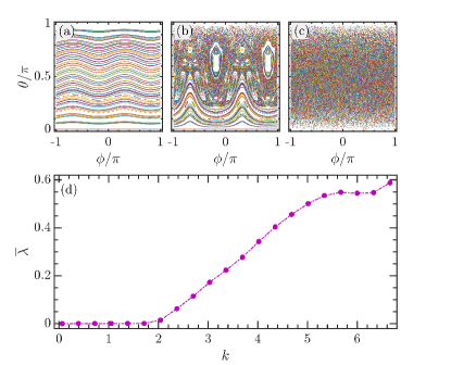
Figure 1: (a)-(c): Phase space portraits of the classical kicked top model for $k=0.4$ (a), $k=2.4$ (b), and $k=6$ (c). The variables ($\theta,\phi$) are plotted for $300$ initial conditions, each with a duration of $300$ kicks. (d) Phase space averaged Lyapunov exponent, $\bar{\lambda}$, as a function of the kick strength $k$. In a numerical simulation, $\bar{\lambda}$ is calculated by averaging over $40000$ trajectories, each evolved for $4000$ kicks. Other parameter: $\alpha=4\pi/11$.

II.1 Classical kicked top model

The classical counterpart of the Heisenberg equation in (II) is obtained in the limit $j\to\infty$. To see this, we define the scaled vector $\mathbf{X}=\mathbf{J}/j$ which obeys the commutation relations $[X_{a},X_{b}]=(1/j)i\epsilon_{abc}X_{c}$. As $j\to\infty$, the vanishing of commutators between the components of $\mathbf{X}$ implies that $X_{a}$ become classical variables. Then, substituting $\mathbf{X}$ into Eq. (II), after some algebra, we find the classical map can be written as

$$\begin{bmatrix}X_{n+1}\\ Y_{n+1}\\ Z_{n+1}\end{bmatrix}=\begin{bmatrix}\cos\alpha&-\sin\alpha&0\\ \sin\alpha\cos\Omega_{n}&\cos\alpha\cos\Omega_{n}&-\sin\Omega_{n}\\ \sin\alpha\sin\Omega_{n}&\cos\alpha\sin\Omega_{n}&\cos\Omega_{n}\end{bmatrix}\begin{bmatrix}X_{n}\\ Y_{n}\\ Z_{n}\end{bmatrix},$$ (8)

where $\Omega_{n}=k(X_{n}\cos\alpha-Y_{n}\sin\alpha)$. The conservation of $\mathbf{J}^{2}$ entails $|\mathbf{X}|^{2}=X^{2}+Y^{2}+Z^{2}=1$. This means that the classical variables $(X,Y,Z)$ lie on the unit sphere and they can be parametrized in terms of the azimuthal angle $\theta$ and polar angle $\phi$ as follows: $X=\sin\theta\cos\phi$, $Y=\sin\theta\sin\phi$, and $Z=\cos\theta$. Hence, the classical phase space is actually two dimensional space described by variables $\theta=\cos^{-1}Z$ and $\phi=\tan^{-1}(Y/X)$.

A prominent feature exhibited by the kicked top model is the transition to chaos as the kicking strength $k$ increases. It is known that the model shows regular behavior in the phase space for lower values of $k$, while increasing $k$ gives rise to the extension of the chaotic regime in the phase space and, therefore, increases the degree of chaos Haake et al. (1987). The emergence of chaos in the dynamics of the classical kicked top with increasing $k$ is clearly observed in Figs. 1(a)-1(c), where the Poincaré sections for several values of $k$ are plotted. One can see that the phase space turns from regular motion for small $k$ to the mixed dynamics with regular regions embedded in the chaotic sea for larger $k$. For even larger $k$, as the $k=6$ case plotted in Fig. 1(c), the phase space is governed by globally chaotic dynamics.

To quantitatively analyze the chaotic properties of the model, we consider the phase space averaged Lyapunov exponent, which measures the degree of chaos in the model and is defined as

$$\bar{\lambda}=\frac{1}{4\pi}\int dS\lambda_{m},$$ (9)

where $dS=\sin\theta d\theta d\phi$ is the phase space area element (or Haar measure) D’Ariano et al. (1992) and $\lambda_{m}$ denotes the largest Lyapunov exponent of the classical map in (8). The largest Lyapunov exponent quantifies the rate of deviation between two nearby orbits in a dynamical system Vallejos and Anteneodo (2002); Jayaraman et al. (2006). For the kicked top model, it can be calculated as D’Ariano et al. (1992); Constantoudis and Theodorakopoulos (1997); Parker and Chua (2012)

$$\lambda_{m}=\ln\left[\lim_{n\to\infty}(t_{m})^{1/n}\right],$$ (10)

where $t_{m}$ represents the largest eigenvalue of $T=\prod_{p=1}^{n}\mathfrak{T}(\mathbf{X}_{p})$ and $\mathfrak{T}(\mathbf{X}_{n})=\partial\mathbf{X}_{n+1}/\partial\mathbf{X}_{n}$ is the tangent map of Eq. (8).

By averaging the largest Lyapunov exponents over different initial conditions in the phase space for various values of $k$, we show the dependence of $\bar{\lambda}$ on the kicking strength $k$ in Fig. 1(d). The regularity of the model at small $k$ leads to the zero value of $\bar{\lambda}$ and it keeps zero up to a certain kicking strength $k_{c}\approx 2$, from which it starts to grow with increasing $k$. Hence, the model undergoes a transition from integrability to chaos as $k$ is increased and the level of chaos is enhanced by increasing the kicking strength.

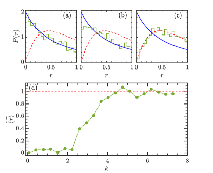
Figure 2: (a)-(c) Distribution of the consecutive level spacing ratios $P(r)$ for $k=0.4$ (a), $k=2.4$ (b), and $k=6$ (c). In each panel, the blue solid and red dashed curves denote the $P_{\mathrm{P}}(r)$ and $P_{\mathrm{WD}}(r)$ [cf. Eq. (12)], respectively. (d) Rescaled average ratio $\widetilde{\langle r\rangle}$ in (14) as a function of the kicking strength $k$. The red dashed horizontal line represents $\widetilde{\langle r\rangle}=1$. Other parameters: $j=2000$ and $\alpha=4\pi/11$.

II.2 Chaos in quantum kicked top model

The chaotic properties discussed above in the classical kicked top model are also manifested in its quantum counterpart. The signatures of quantum chaos can be captured by several probes, including the statistics of eigenvalues and eigenvectors Brody et al. (1981); Zyczkowski (1990), the dynamical behavior of the Loschmidt echo Emerson et al. (2002); Torres-Herrera and Santos (2017b), the entanglement dyanmics Wang et al. (2004); Gietka et al. (2019); Piga et al. (2019), the out-of-time-ordered correlators García-Mata et al. (2018); Fortes et al. (2019); Lantagne-Hurtubise et al. (2020), quantum coherence Anand et al. (2021), and the operator complexity Magán (2018); Bhattacharyya et al. (2021); Rabinovici et al. (2022), to name a few. Here, in order to unveil the fingerprint of chaos in the quantum kicked top model, we study the spectral properties of the Floquet operator based on the level spacing ratios $r_{n}$, defined as Oganesyan and Huse (2007); Atas et al. (2013a)

$$r_{n}=\frac{\mathrm{min}(d_{n},d_{n+1})}{\mathrm{max}(d_{n},d_{n+1})}={\mathrm{min}(w_{n},\frac{1}{w_{n}})},$$ (11)

where $d_{n}=\mu_{n+1}-\mu_{n}$ is the spacing between two successive levels with $\mu_{n}$ being the $n$th eigenphase of the Floquet operator, and $w_{n}=d_{n+1}/d_{n}$. Clearly, the definition of $r_{n}$ implies that it varies in the interval $r_{n}\in[0,1]$. As $r_{n}$ does not rely on the local density of states, the calculation of its distribution is not required to perform the so-called unfolding procedure, which is known to be intricate Gómez et al. (2002); Corps and Relaño (2021). This makes the level spacing ratio $r_{n}$ a convenient chaos indicator in the studies of quantum chaos, in particular for quantum many-body chaotic systems.

It has been demonstrated that the distribution of $r_{n}$, denoted by $P(r)$, can be used to distinguish between integrable and chaotic systems Oganesyan and Huse (2007); Atas et al. (2013a). In particular, the analytical expression of $P(r)$ has been obtained for both integrable (Poisson statistics) and chaotic (Wigner-Dyson statistics) spectra, given by Atas et al. (2013a, b); Giraud et al. (2022)

$$P_{\mathrm{P}}(r)=\frac{2}{(1+r)^{2}},\ P_{\mathrm{WD}}(r)=\frac{27}{4}\frac{r+r^{2}}{(1+r+r^{2})^{5/2}}.$$ (12)

The distributions of level spacing ratios $P(r)$ of the Floquet operator for several values of $k$ are shown in Figs. 2(a)-2(c), where we also compare our numerical results to the analytical formula of $P(r)$ in Eq. (12). We see that $P(r)$ follows the distribution for Poisson statistics $P_{\mathrm{P}}(r)$ for small $k$ [Fig. 2(a)]. This means the absence of level repulsions in the model are consistent with the regular structure of the phase space. As $k$ is increased, $P(r)$ deviates from $P_{\mathrm{P}}(r)$ and has a Poisson-like tail, as observed in Fig. 2(b). This indicates the highly localized weak correlations between eigenphases corresponding to the mixed feature in the phase space. Finally, for the case of strong kicking strength, as shown in Fig. 2(c), the ratio distribution $P(r)$ is in good agreement with $P_{\mathrm{WD}}(r)$ suggesting level repulsion in the fully chaotic regime. The changes in the behaviors of the distribution $P(r)$ clearly confirms the integrablity-to-chaos transition in the kicked top model. It is worthwhile to mention that the level statistics for the Floquet operator in the chaotic regime should belong to random matrices of the circular orthogonal ensemble (COE). However, since the COE statistics is asymptotically described by the random matrices belonging to the Gaussian orthogonal ensemble (GOE) in the thermodynamic (also semiclassical) limit D’Alessio and Rigol (2014), we have therefore compared our numerical results to the GOE counterpart.

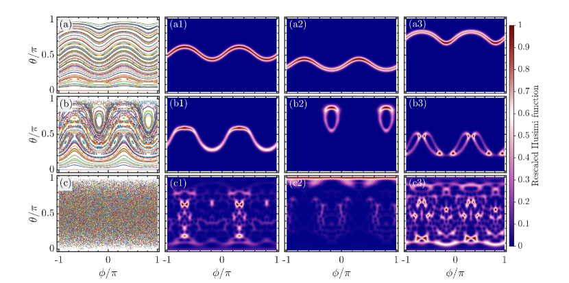
Figure 3: (a)-(c): Phase portraits of the classical kicked top model for (a) $k=1$, (b) $k=2$, and (c) $k=7$. Here, $300$ randomly chosen initial conditions in the phase space have been plotted after $300$ kicks. (a1)-(a3): Husimi function rescaled by its maximum value for the eigenstates of $\mathcal{F}$ with eigenphases (a1) $\mu\approx-2.9$, (a2) $\mu\approx-2.19$, and (a3) $\mu\approx 2.17$ for $k=1$. (b1)-b(3): Husimi function rescaled by its maximum value for the eigenstates of $\mathcal{F}$ with same eigenphases as in (a1)-a(3) for $k=2$. (c1)-c(3): Husimi function rescaled by its maximum value for the eigenstates of $\mathcal{F}$ with same eigenphases as in (a1)-a(3) for $k=7$. Other parameters are: $\alpha=4\pi/11$ and $j=150$.

Instead of focusing on the ratio distribution $P(r)$, the crossover from integrable to chaos in the model can also be captured by the mean level spacing ratio $\langle r\rangle$, defined as

$$\langle r\rangle=\frac{1}{\mathcal{N}}\sum_{n=1}^{\mathcal{N}}r_{n},$$ (13)

where $\mathcal{N}$ denotes the total number of $r_{n}$. For integrable systems, the Poisson statistics yields $\langle r\rangle_{P}\approx 0.39$ Atas et al. (2013a), while for the chaotic systems with Wigner-Dyson statistics, the mean value $\langle r\rangle_{WD}\approx 0.53$ Atas et al. (2013a); Giraud et al. (2022); D’Alessio and Rigol (2014). It is more convenient to consider the rescaled average level spacing ratio Łydżba and Sowiński (2022):

$$\widetilde{\langle r\rangle}=\frac{\left|\langle r\rangle-\langle r\rangle_{P}\right|}{\langle r\rangle_{WD}-\langle r\rangle_{P}}.$$ (14)

It is defined in the range $0\leq\widetilde{\langle r\rangle}\leq 1$, with two limiting values corresponding to the Poisson and Wigner-Dyson distributions, respectively. Figure 2(d) illustrates how $\widetilde{\langle r\rangle}$ varies as a function of the kicking strength $k$. The transition to chaos with increasing $k$ is evidently revealed by the interpolation of $\widetilde{\langle r\rangle}$ between Poisson and Wigner-Dyson cases. We further note that the upturn in $\widetilde{\langle r\rangle}$ with increasing $k$ is in agreement with that of the phase space averaged Lyapunov exponent in Fig. 1(d), indicating a good quantum-classical correspondence.

III Statistics of the phase space localization measures

The transition to chaos also correlates with a remarkable change in the structure of eigenstates. To analyze the structure of eigenstates, it is necessary to decompose them in a certain basis. The choice of basis is usually determined by the system and the physical question under consideration. In this work we aim to explore the properties of the phase space localization. A natural choice for us is the basis consisting of the coherent states $|\theta,\phi\rangle$, as they are as close as possible to the classical phase points due to their minimal uncertainty. For the kicked top model, the coherent states are the generalized $\mathrm{SU}(2)$ spin coherent states, which are generated by rotating the Dicke state $|j,j\rangle$ as follows Gazeau (2009); Zhang et al. (1990); Antoine et al. (2018):

$$|\theta,\phi\rangle =\exp[i\theta(J_{x}\sin\phi-J_{y}\cos\phi)]|j,j\rangle,$$

$$=\sum_{m=-j}^{m=j}\frac{\tau^{j-m}}{(1+|\tau|^{2})^{j}}\sqrt{\frac{(2j)!}{(j-m)!(j+m)!}}|j,m\rangle,$$ (15)

with $\tau=\tan(\theta/2)e^{i\phi}$ and $\theta\in[0,\pi),\phi\in[-\pi,\pi)$. The coherent states basis $\{|\theta,\phi\rangle\}$ is overcomplete with the closure relation

$$\mathds{1}=\frac{2j+1}{4\pi}\int d\theta d\phi\sin\theta|\theta,\phi\rangle\langle\theta,\phi|.$$ (16)

The expansion of the $n$th eigenstate $|\mu_{n}\rangle$ of $\mathcal{F}$ in the basis $\{|\theta,\phi\rangle\}$ can be written as

$$|\mu_{n}\rangle=\frac{2j+1}{4\pi}\int d\theta d\phi\sin\theta p_{n}(\theta,\phi)|\theta,\phi\rangle,$$ (17)

where $p_{n}(\theta,\phi)=\langle\theta,\phi|\mu_{n}\rangle$ is the overlap between the coherent state $|\theta,\phi\rangle$ and the $n$th eigenstate $|\mu_{n}\rangle$. Then, valuable information about the structure of the $n$th eigenstate in the phase space is provided by the Husimi function, defined as the square of $p_{n}(\theta,\phi)$ module,

$$Q_{n}(\theta,\phi)=|p_{n}(\theta,\phi)|^{2}=\langle\theta,\phi|\rho_{n}|\theta,\phi\rangle,$$ (18)

with $\rho_{n}=|\mu_{n}\rangle\langle\mu_{n}|$ and it satisfies the normalization condition

$$\frac{2j+1}{4\pi}\int d\theta d\phi\sin\theta Q_{n}(\theta,\phi)=1.$$ (19)

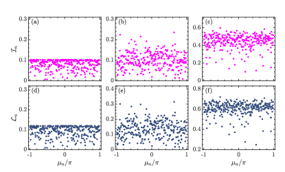
Figure 4: (a)-(c): Inverse participation ratio $\mathcal{I}_{n}$ of the eigenstates for the kicked top model as a function of eigenphases $\mu_{n}$ of the Floquet operator for (a) $k=0.4$, (b) $k=2.4$, and (c) $k=6$. (d)-(f): Localization measure $\mathcal{L}_{n}$ for the eigenstates of the kicked top model as a function of eigenphases $\mu_{n}$ of the Floquet operator for the same values of $k$ as in panels (a)-(c). Other parameters: $\alpha=4\pi/11$ and $j=150$.

The Husimi functions of various eigenstates of $\mathcal{F}$ for several values of $k$ are plotted in Fig. 3 with associated classical phase portraits, in agreement with the principle of uniform semiclassical condensation (PUSC) of the Wigner functions or Husimi functions - see Robnik (1998); Lozej et al. (2022); Veble et al. (1999) and references therein. (Husimi function also is a Gaussian smoothed Wigner function.) We first note that the Husimi functions show a good correspondence to the classical phase space orbits. This is due to the fact that the coherent states represent the closest quantum analog of the classical phase space points. Meanwhile, the good agreement between the Husimi function and the classical phase space structure also confirms that the coherent state basis is an appropriate basis for investigating the phase space localization. We further observe the degree of localization of the Husimi function in the phase space depending on the kicking strength. In particular, even in deep chaotic regime, there still exist some eigenstates that are highly localized in the phase space, such as the one illustrated in Fig. 3(c2).

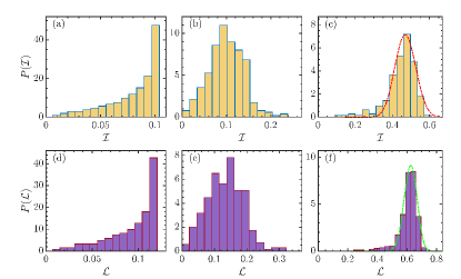
Figure 5: (a)-(c): Distribution of $\mathcal{I}_{n}$ for (a) $k=0.4$, (b) $k=2.4$, and (c) $k=6$. In panel (c), the red dot-dashed line denotes the beta distribution (23) with $(x_{min},x_{max})=(0.145,0.872)$ and the shape parameters are $a=18.9435$ and $b=23.3284$. (d)-(f): Distribution of $\mathcal{L}_{n}$ for the same values of $k$ as in panels (a)-(c). The green dot-dashed line in panel (f) represents the beta distribution (23) with $(x_{min},x_{max})=(0.219,0.8849)$ and the shape parameters $(a,b)=(33.7363,21.8592)$. Other parameter: $\alpha=4\pi/11$ and $j=150$.

To measure the degree of localization of the $n$th eigenstate of $\mathcal{F}$ in the basis $\{|\theta,\phi\rangle\}$, we consider two different localization measures based on the Husimi function. The first one is the well-known inverse participation ratio, which measures how many basis states the quantum state occupies Evers and Mirlin (2008). In terms of Husimi function, the inverse participation ratio for the $n$th eigenstate is defined as

$$\mathcal{I}_{n}=\left[\mathcal{N}_{c}\frac{2j+1}{4\pi}\int d\theta d\phi\sin\theta Q_{n}^{2}(\theta,\phi)\right]^{-1},$$ (20)

where $\mathcal{N}_{c}=(2j+1)/(4\pi)\int d\theta d\phi\sin\theta=2j+1$ acts as the normalization constant. The second localization measure is defined through the Wehrl entropy Wehrl (1978) and for the $n$th eigenstate it is given by Batistić and Robnik (2013); Wang and Robnik (2020); Lozej et al. (2022)

$$\mathcal{L}_{n}=\frac{\exp(S_{W})}{\mathcal{N}_{c}},$$ (21)

where

$$S_{W}=-\frac{2j+1}{4\pi}\int d\theta d\phi\sin\theta Q_{n}(\theta,\phi)\ln[Q(\theta,\phi)],$$ (22)

is the Wehrl entropy. In the semiclassical limit with $j\to\infty$, both localization measures interpolate between two extreme ends: the uttermost localized eigenstates with $\mathcal{I}_{n}=\mathcal{L}_{n}=0$ and the fully delocalized chaotic eigenstates with $\mathcal{I}_{n}=\mathcal{L}_{n}=1$ Wang and Pérez-Bernal (2021); Lozej et al. (2022). In the former case $Q_{n}$ is localized on a small region of size $\Delta S$ and is constant there, so that $\mathcal{I}_{n}$ and $\mathcal{L}_{n}$ go to zero as $\Delta S$ tends to zero. In the latter case $Q_{n}$ is constant and equal to its average value $\bar{Q}_{n}=1/(2j+1)$.

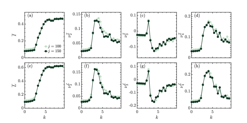
Figure 6: (a) Mean value $\bar{I}$, (b) Standard deviation $\nu_{2}^{\mathcal{I}}$, (c) Cube root of the third central moment $\nu_{3}^{\mathcal{I}}$, and (d) $\nu_{4}^{\mathcal{I}}$, obtained from Eq. (24), as a function of $k$ for several system sizes, see the legend in panel (a). Dependence on $k$ of (e) mean value $\bar{L}$, (f) standard deviation $\nu_{2}^{\mathcal{L}}$, (g) cube root of the third central moment $\nu_{3}^{\mathcal{L}}$, and (h) $\nu_{4}^{\mathcal{L}}$, calculated by Eq. (24), for the same system sizes as legend in panel(a). Other parameter: $\alpha=4\pi/11$.

In the following of this section, we will focus on both the individual and joint statistics of these localization measures. The purpose of our study is to unveil the impact of chaos on the structure of eigenstates and to identify the signatures of chaos in the statistical properties of the phase space localization measures.

III.1 Statistics of $\mathcal{I}_{n}$ and $\mathcal{L}_{n}$

Let us consider the statistics of the localization measures $\mathcal{I}_{n}$ and $\mathcal{L}_{n}$. In Fig. 4, we plot $\mathcal{I}_{n}$ and $\mathcal{L}_{n}$ as a function of $\mu_{n}$ for different values of $k$. As both $\mathcal{I}_{n}$ and $\mathcal{L}_{n}$ measure the degree of (de)localization of an eigenstate in the phase space, one can expect that they should behave in a similar way as a function of eigenphases. This is confirmed by our numerical results which show overall similarities between the behaviors of $\mathcal{L}_{n}$ and $\mathcal{I}_{n}$. We see that the values of $\mathcal{I}_{n}$ and $\mathcal{L}_{n}$ are low and concentrated in a narrow range for small $k$ [see Figs. 4(a) and 4(d)], suggesting that the eigenstates are localized in the phase space reflecting the regular dynamics in the classical case. Moreover, there is an obvious concentration in $\mathcal{I}_{n}$ and $\mathcal{L}_{n}$ around their corrresponding maximal values. A careful check shows that these sharp upper limits of the localization measures can only be seen in the regular regime and are associated with the eigenstates that correspond to the classical orbits located in an interval with $\pi/4\lesssim\theta\lesssim 3\pi/4$. It should be observed that the thickness of the Husimi function localized on an invariant torus of length $\approx 2\pi$ is of the order of the square root of the effective Planck constant $\hbar_{eff}\approx 1/j$, which determines the maximum value of $\mathcal{I}_{n}$ and $\mathcal{L}_{n}$. This is of course in contradistinction of the chaotic eigenstates.

As $k$ is increased, the values of localization measures also increase, but the eigenstates with high and low values of the localization measures are coexisting in the spectrum, as illustrated in Figs. 4(b) and 4(e). This means that the degree of localization has strong fluctuations among the eigenstates. The reason can be attributed to the mixed feature exhibited by the corresponding classical dynamics, in agreement with PUSC. The eigenstates associated with the regular islands are highly localized states with low-$\mathcal{I}_{n}/\mathcal{L}_{n}$, while the high-$\mathcal{I}_{n}/\mathcal{L}_{n}$ values stem from the eigenstates that are located in the chaotic sea. At large values of $k$, as plotted in Figs. 4(c) and 4(f), the values of $\mathcal{I}_{n}$ and $\mathcal{L}_{n}$ are much larger. This is due to the fact that the system becomes classically globally chaotic, which leads to the eigenstates being spread over the whole phase space. However, there are still some low-$\mathcal{I}_{n}/\mathcal{L}_{n}$ eigenstates, which are the localized chaotic eigenstates, as observed in Fig. 3(c2). For a phenomenological analysis of Husimi functions in a mixed-type regime see Lozej et al. (2022) and references therein.

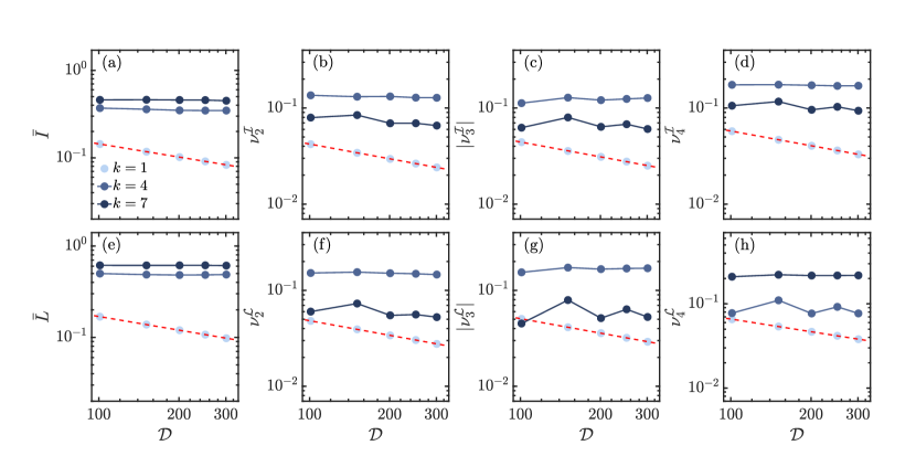
Figure 7: Dependence on the Hilbert space dimension $\mathcal{D}$ of (a) mean value $\bar{I}$, (b) standard deviation $\nu_{2}^{\mathcal{I}}$, (c) cube root of the third central moment $|\nu_{3}^{\mathcal{I}}|$, (d) $\nu_{4}^{\mathcal{I}}$ [cf. Eq. (24)] (e) mean value $\bar{L}$, (f) $\nu_{2}^{\mathcal{L}}$, (g) $\nu_{3}^{\mathcal{L}}$ and (h) $\nu_{4}^{\mathcal{L}}$ [cf. Eq. (24)] for several kicking strengths $k$, see legend in panel (a). The red dashed line in each panel corresponds to fitting curve of the power law $\propto\mathcal{D}^{-\gamma}$ with $\gamma\approx 0.5$, to the data of $k=1$ case. Other parameter: $\alpha=4\pi/11$.

The visible different scatter plots in Fig. 4 imply that the localization measures of eigenstates would have different statistical properties in the regular and chaotic regimes. To verify this statement, we study the distribution of the localization measures, denoted by $P(\mathcal{I})$ and $P(\mathcal{L})$, which are, respectively, defined as the probability to find $\mathcal{I}_{n}$ and $\mathcal{L}_{n}$ in an infinitesimal interval $[\mathcal{I},\mathcal{I}+d\mathcal{I}]$ and $[\mathcal{L},\mathcal{L}+d\mathcal{L}]$.

Figure 5 plots $P(\mathcal{I})$ and $P(\mathcal{L})$ for the same values of $k$ as in Fig. 4. One can clearly see that the behaviors of $P(\mathcal{I})$ and $P(\mathcal{L})$ are very similar. In particular, both of them undergo a drastic change in their property with increasing $k$. Specifically, in a regular regime with small $k$, the values of $\mathcal{I}_{n}$ and $\mathcal{L}_{n}$ distribute over a narrow range and are sharply concentrated near $0.1$ and 0.12, respectively. As a consequence, both $P(\mathcal{I})$ and $P(\mathcal{L})$ have a small width and exhibits a sharp peak around the upper limit of $\mathcal{I}_{n}$ and $\mathcal{L}_{n}$, as shown in Figs. 5(a) and 5(d) [note the scale of the y-axis]. Increasing the kicking strength $k$ tends to increase the width of $P(\mathcal{I})$ and $P(\mathcal{L})$, as well as shifting the location of the peaks in them to larger values of $\mathcal{I}_{n}$ and $\mathcal{L}_{n}$. The distributions of localization measures in the chaotic regime are asymmetric or skewed with a peak close to their largest values, as evident from Figs. 5(e) and 5(f). The asymmetry shape of $P(\mathcal{I})$ and $P(\mathcal{L})$ is a consequence of the low-$\mathcal{I}_{n}/\mathcal{L}_{n}$ localized eigenstates.

Inspired by our previous works Batistić et al. (2019); Lozej et al. (2022); Wang and Robnik (2020), in which the distribution of $\mathcal{L}_{n}$ for the delocalized eigenstates in several chaotic systems has been investigated, here we explore whether the distributions $P(\mathcal{I})$ and $P(\mathcal{L})$ for the delocalized eigenstates can be well described by the beta distribution Evans et al. (2011)

$$P_{\beta}(x)=\frac{(x-x_{min})^{a-1}(x_{max}-x)^{b-1}}{(x_{max}-x_{min})^{a+b-1}B(a,b)},$$ (23)

where $x_{min}\leq x\leq x_{max}$, $a$ and $b$ are the shape parameters, and $B(a,b)=\int_{0}^{1}x^{a-1}(1-x)^{b-1}dx$ is the beta function.

The best fitted beta distribution of $P(\mathcal{I})$ is shown in Fig. 5(c). The minimal and maximal values of $x$ of our fitted beta distribution are empirically found to be $x_{min}=0.145$ and $x_{max}=0.872$, respectively. Unlike in our previous works, here we fit the distribution on the interval $[x_{min},x_{max}]$, but note that the actual range of numerically obtained $\mathcal{I}_{n}$ is on the interval $[0.1016,0.5975]$. The maximal value $\mathcal{I}_{n,max}=0.5975$ agrees with the findings in other systems. Here, the energy is fixed by $j$. On the other hand, the distribution $P(\mathcal{L})$ is well captured by the beta distribution fitted on the interval $[x_{min},x_{max}]=[0.219,0.8849]$, as demonstrated in Fig. 5(f). We also note that the data of $\mathcal{L}_{n}$ are in the range $[0.2479,0.7206]$. Thus, the maximal $\mathcal{L}_{n}$ is found to be $\mathcal{L}_{n,max}=0.7206$, which is roughly consistent with other systems. The fact that the fit by the beta distribution is not perfect should be attributed to the structure of the chaotic sea in the sense of some stickiness regions which so far have not been detected.

In fact, more generally, it appears phenomenologically that chaotic quantum eigenstates exhibit the beta distribution for the localization measures, provided they are classically uniformly chaotic without significant stickiness regions. In doing this we consider the eigenstates within a small energy interval, small enough to have a well defined regime and at the same time large enough to have a reasonable statistics. This has been demonstrated first in the mixed-type billiard introduced by Robnik Batistić et al. (2019), and also in the stadium billiard of Bunimovich, in the lemon billiards introduced by Heller and Tomsovic (see Refs. Lozej et al. (2021a, 2022) and references therein) and in the Dicke model Wang and Robnik (2020). Therefore, we believe that this distribution of localization measure is universal. However, if the the chaotic region has significant stickiness regions such as, e.g., in the ergodic lemon billiard Lozej et al. (2021b), we see nonuniversal deviations from the beta distribution.

To quantify the above observed features in the distributions of $\mathcal{I}_{n}$ and $\mathcal{L}_{n}$, as well as to quantitatively assess the degree of similarity between them, we consider the mean and the $m$th root of the $m$th central moment of $P(\mathcal{O}_{q})(q=1,2)$:

$$\overline{O_{q}}=\frac{1}{\mathcal{D}}\sum_{n}\mathcal{O}_{q,n},\ \nu_{m}^{\mathcal{O}_{q}}=\left[\frac{1}{\mathcal{D}}\sum_{n}(\mathcal{O}_{q,n}-\overline{O_{q}})^{m}\right]^{1/m},$$ (24)

where $\mathcal{O}_{1}$ denotes $\mathcal{I}$, $\mathcal{O}_{2}$ represents $\mathcal{L}$, and $\mathcal{D}=j+1$ is the Hilbert space dimension. As the zeroth central moment is equal to one and the first central moment is zero, we are, therefore, mainly interested in $m=2,3,4$, the standard deviation, cube root of the skewness, and the fourth root of kurtosis of the distribution, respectively.

Figure 6 plots these quantities as a function of $k$ for several system sizes $j$. The onset of chaos can be clearly identified from the sharp growth behavior displayed by these quantities. Remarkably, the drastic growing point of these quantities with increasing $k$ are in agreement with that of average Lyapunov exponent $\bar{\lambda}$ in Fig. 1(d) and average gap ratio $\langle r\rangle$ in Fig. 2(d). As $\nu_{2,3,4}^{\mathcal{O}_{q}}$ quantify the fluctuation, the skewness, and the tailedness of the corresponding distribution, the non-zero values of them in the chaotic regime imply that the distribution $P(\mathcal{O}_{q})$ is asymmetrical, consistent with the result shown in Figs. 5(c) and 5(f). Moreover, we also note that our considered quantities are only weakly dependent on the system size $j$ in the chaotic and regular regime. However, on the other hand, they are independent of the kicking strength $k$ in the regular regime.

The dependence of these quantities with varying the Hilbert space dimension $\mathcal{D}$ for different system sizes are plotted in Fig. 7. Notice that we consider the absolute value of $\nu_{3}^{\mathcal{O}_{q}}$ rather than $\nu_{3}^{\mathcal{O}_{q}}$ itself in our numerical simulation. One can see that all these quantities remain almost unchanged with increasing $\mathcal{D}$ for the case with large $k$, wherease they all decrease with increasing $\mathcal{D}$ for the case of $k=1$. Moreover, we find that their decreasing with $\mathcal{D}$ follows the same power law of the form $y=C_{y}\mathcal{D}^{-\gamma}$ with $\gamma\approx 0.5$. This is explained by the fact that the Husimi function associated with an invariant torus has roughly length $2\pi$ and thickness $\approx\sqrt{\hbar_{eff}}=1/\sqrt{j}$. This suggests that all of them vanish as $\mathcal{D}\to\infty$ and the distributions $P(\mathcal{I})$ and $P(\mathcal{L})$ become the $\delta$-distribution, $P(\mathcal{I})=\delta(\mathcal{I}),P(\mathcal{L})=\delta(\mathcal{L})$, as expected. It should be observed that according to the Figs. 6 and 7 in the chaotic regime the average value of $\mathcal{O}_{q}$ has converged to its semiclassical limit $j\rightarrow\infty$, while $\nu_{2}^{\mathcal{O}q}$, the standard deviation, seems to decay very slowly with $j$ to its expected semiclassical limit $\nu_{2}^{\mathcal{O}_{q}}=0$. The case $k=4$ shows no decay with $\mathcal{D}=j+1$, probably because it is still a mixture of a large chaotic component and a small regular component.

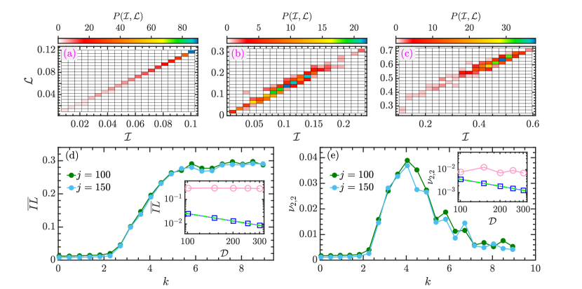
Figure 8: Joint probability distribution $P(\mathcal{I},\mathcal{L})$ of the kicked top model for $k=0.4$ (a), $k=2.4$ (b), and $k=6$ (c) with $j=150$. (d) Dependence of $\overline{IL}$ [cf. Eq. (25)] on the kicking strength $k$ for different system sizes $j$. Inset: Scaling of $\overline{IL}$ with Hilbert space dimension $\mathcal{D}$ for $k=1$ (blue squares) and $k=7$ (pink circles). The green dashed line in the inset marks the scaling $\overline{IL}\sim\mathcal{D}^{-1}$. (e) Evolution of $\nu_{2,2}$ [cf. Eq. (25)] versus the kicking strength $k$ for several system sizes $j$. The inset plots $\nu_{2,2}$ as a function of $\mathcal{D}$ for $k=1$ (blue squares) and $k=7$ (pink circles). In the inset, the green dashed line denotes the decay $\nu_{2,2}\sim\mathcal{D}^{-\zeta}$ with $\zeta=1$. Other parameter: $\alpha=4\pi/11$.

III.2 Joint probability distribution of the localization measures

We finally discuss the interplay between the onset of chaos and the properties of the joint probability distribution of the localization measures. The above revealed statistical properties of the individual localization measure distributions indicate that the statistics of the localization measures provides useful information about the structure of the eigenstates and can detect the onset of chaos. Further insights into the characteristics of the eigenstates and the signatures of quantum chaos can be obtained from the joint probability distribution $P(\mathcal{I},\mathcal{L})$, which is defined as the probability to find $\mathcal{I}$ and $\mathcal{L}$ in an infinitesimal box $[\mathcal{I},\mathcal{I}+d\mathcal{I}]\times[\mathcal{L},\mathcal{L}+d\mathcal{L}]$.

The joint distribution $P(\mathcal{I},\mathcal{L})$ of the kicked top model for various values of the kicking strength $k$ are shown in Figs. 8(a)-8(c). For the regular case with $k=1$, the distribution $P(\mathcal{I},\mathcal{L})$ distributes over the small values of $\mathcal{I}$ and $\mathcal{L}$ with a very narrow width in the $\mathcal{I}\mathcal{L}$ plane [Fig. 8(a)]. As the kicking strength $k$ increases, the joint distribution extends out to large $\mathcal{I}$ and $\mathcal{L}$. Moreover, the width of the distribution $P(\mathcal{I},\mathcal{L})$ also increases with increasing $k$, as seen in Figs. 8(b) and 8(c). However, we note that the largest width of $P(\mathcal{I},\mathcal{L})$ occurs in the mixed regime, instead of the fully chaotic case. In fact, most of the eigenstates are delocalized in strong chaotic regime, both $\mathcal{I}$ and $\mathcal{L}$ are concentrated around some large values, resulting in small width of the joint distribution $P(\mathcal{I},\mathcal{L})$. It has been found already in Ref. Batistić et al. (2020) that the two localization measures, after a proper normalization, are nearly linearly related.

The observed characters of $P(\mathcal{I},\mathcal{L})$ can be quantified by the following mixed moments,

$$\overline{IL}=\frac{1}{\mathcal{D}}\sum_{n}\mathcal{I}_{n}\mathcal{L}_{n},\ \nu_{2,2}=\left[\frac{1}{\mathcal{D}}\sum_{n}(\mathcal{I}_{n}-\bar{I})(\mathcal{L}_{n}-\bar{L})\right]^{1/2},$$ (25)

where $\mathcal{D}=j+1$ is the Hilbert space dimension, and $\bar{I}$ and $\bar{L}$ are the mean values of $\mathcal{I}_{n}$ and $\mathcal{L}_{n}$ in Eqs. (24). The evolution of these quantities as a function of $k$ is depicted in Figs. 8(d) and 8(e). Clearly, we see that the transition to chaos also leaves an imprint in the joint distibution of the localization measures and the onset of chaos with increasing kicking strength can be unveiled unambiguously by the upturn of these quantities as $k$ increases. Furthermore, we also find that the values of these quantities are almost independent of the system size for the chaotic case, while in the regular regime they decrease with increasing system size and are decaying as $\sim\mathcal{D}^{-\zeta}$ with $\zeta\approx 1$, as demonstrated in the insets of Figs. 8(d) and 8(e). Again, this is due to the expected proportionality of these quantities to the effective Planck constant $\hbar_{eff}\approx 1/j$. Hence, in the regular regime, the joint distribution approaches the Dirac $\delta$-distribution as $j\to\infty$, in agreement with the asymptotic behaviors of $P(\mathcal{I})$ and $P(\mathcal{L})$. Here, again we may emphasize that the average value $\overline{IL}$ in the chaotic regime has converged to its semiclassical value as $j\rightarrow\infty$, while the standard deviation $\nu_{2,2}$ decays very slowly with $j$.

IV Conclusion

In this work, the phase space localization properties of the eigenstates have been scrutinized in the kicked top model that undergoes a transition to chaos with increasing the kicking strength. The information about the phase space localization of the eigenstates is encoded in the associated Husimi functions, which exhibit distinct localization features depending on whether the system is regular or chaotic. Hence, the emergence of chaos bears a significant change in the eigenstates and the crossover from integrability/regularity to quantum chaos can be probed by the localization characters of eigenstates in phase space. Remarkably, we have again found that there still exist some localized eigenstates even in the deep chaotic regime, which is a manifestation of quantum dynamical localization, and the localization measures exhibit the beta distribution.

The notably different localization behavior of the Husimi function in regular and chaotic regime has led to a characterization of the phase space localization phenomenon of eigenstates in terms of two different localization measures, i. e., the inverse participation ratio and the Wehrl entropy, that are based on the Husimi function. The investigation of the statistics of the localization measures reveals that their distributions are sharply peaked around some small values in the regular regime, indicating that the eigenstates are highly localized states in the phase space, spanned by the invariant tori in the classical phase space. As the system tends from integrability/regularity toward chaos, the width of their distributions is increased and the peak of the distributions is moved to the large values of the localization measures. The scenario is in line with the predictions of the Principle of Uniform Semiclassical Condensation (PUSC) of the Husimi (or Wigner) functions, in the semiclassical limit. However, we have found that the distribution of the localization measures also displays fluctuations in the deep chaotic regime. In fact, the distribution of the localization measure approaches the beta distribution, in agreement with previous works Lozej et al. (2022), and in the ultimate semiclassical limit is expected to tend to the Dirac delta distribution. In this ultimate limit (not yet seen in this study) most of eigenstates of the fully chaotic system are then expected to be uniformly delocalized in the phase space. Thus, the features shown by the distributions of the localization measures certainly confirm their usefulness to detect the onset of chaos.

To capture the quantitative features of the distributions of the localization measures, we also consider the central moments of the distributions. We have demonstrated that the central moments are sensitive to the presence of chaos, which results in a drastic change in the behaviors of the central moments. We therefore verified that the statistical properties of the localization measures are the useful witnesses of chaos. In particular, as we showed, the transition to chaos provided by the central moments is in good agreement with the classical case. Further analysis on the scaling of the central moments reveals that the distribution of the localization measures in the regular regime is approaching the Dirac delta distribution in the classical limit, as expected, while in the fully chaotic regime in the same limit it approaches the delta distribution peaked at the maximal value of the localization measure. This approach seems to be extremely slow.

The results presented in this work provide more insights into the relationship between the phase space structure of eigenstates and the onset of chaos in quantum systems. Unveiling how the statistics of the localization measures of eigenstates is affected by underlying chaos would help us get deep understanding on the signatures of quantum chaos and opens up a new way to distinguish between regular and chaotic dynamics in quantum systems. An interesting extension of this work is to explore how our results change in the many body quantum chaotic systems, such as the coupled top model Mondal et al. (2020), Dicke model Wang and Robnik (2020); Villaseñor et al. (2021); Pilatowsky-Cameo et al. (2022), and Bose-Hubbard model Pausch et al. (2021a); Fogarty et al. (2021); Wittmann W. et al. (2022). Another open question that deserves examination is to study the correlation between the phase space localization measures and the entanglement entropy in quantum chaotic systems.

Appendix: A short derivation of the formulae (II)

The discrete mapping of the the Heisenberg operators $\mathbf{J}=(J_{x},J_{y},J_{z})$ is a composition of two mappings: the first one is a free precessional rotation (between two torsional kicks) by the angle $\alpha$ around the $z$ axis, namely $\bar{J_{\ell}}=\exp(i\alpha J_{z})\;J_{\ell}\;\exp(-i\alpha J_{z})$ with $\ell=x,y,z$. Using the Campbell identity [Eq. (6)] and the commutation relations for $\mathbf{J}=(J_{x},J_{y},J_{z})$ we find immediately that

$$\bar{J_{z}}=J_{z},\;\;\;(\bar{J}_{x}+i\bar{J}_{y})=(J_{x}+iJ_{y})\exp(i\alpha).$$ (26)

The other mapping is due to a torsional kick, which appears periodically with period one, generated by $\bar{J_{\ell}}=\exp(i\omega J_{x}^{2})\;J_{\ell}\;\exp(-i\omega J_{x}^{2})$, where $\omega=k/(2j)$. When applying again the Campbell identity, we first note that, using the commutation relations for $\mathbf{J}=(J_{x},J_{y},J_{z})$ , the following commutator is found to be $[J_{x}^{2},(J_{y}+iJ_{z})(2J_{x}+1)^{n}]=(J_{y}+iJ_{z})(2J_{x}+1)^{(n+1)}$, for all nonnegative $n=0,1,2,\dots$, and therefore,

$$\bar{J_{x}}=J_{x},\;\;\;(\bar{J}_{y}+i\bar{J}_{z})=(J_{y}+iJ_{z})\exp(i\omega(2J_{x}+1)).$$ (27)

Compositum of the two mappings results in the transformation in Eq. (II).

References

- Haake (2010) F. Haake, Quantum Signatures of Chaos (Springer, Berlin Heidelberg, 2010).
- Stöckmann (1999) H.-J. Stöckmann, Quantum chaos: an introduction (Cambridge University Press, 1999).
- Nandkishore and Huse (2015) R. Nandkishore and D. A. Huse, Ann. Rev. Condens. Matter Phys. 6, 15 (2015).
- D’Alessio et al. (2016) L. D’Alessio, Y. Kafri, A. Polkovnikov, and M. Rigol, Adv. Phys. 65, 239 (2016).
- Borgonovi et al. (2016) F. Borgonovi, F. Izrailev, L. Santos, and V. Zelevinsky, Phys. Rep. 626, 1 (2016).
- Deutsch (2018) J. M. Deutsch, Rep. Prog. Phys. 81, 082001 (2018).
- Maldacena et al. (2016) J. Maldacena, S. H. Shenker, and D. Stanford, J. High Energ. Phys. 2016, 106 (2016).
- Kos et al. (2018) P. Kos, M. Ljubotina, and T. Prosen, Phys. Rev. X 8, 021062 (2018).
- Jahnke (2019) V. Jahnke, Adv. High Energ. Phys. 2019, 9632708 (2019).
- Bertini et al. (2019) B. Bertini, P. Kos, and T. Prosen, Phys. Rev. X 9, 021033 (2019).
- Lerose and Pappalardi (2020) A. Lerose and S. Pappalardi, Phys. Rev. A 102, 032404 (2020).
- Lichtenberg and Lieberman (2013) A. J. Lichtenberg and M. A. Lieberman, Regular and chaotic dynamics, Vol. 38 (Springer Science & Business Media, 2013).
- Cvitanovic et al. (2005) P. Cvitanovic, R. Artuso, R. Mainieri, G. Tanner, G. Vattay, N. Whelan, and A. Wirzba, ChaosBook. org (Niels Bohr Institute, Copenhagen 2005) 69, 25 (2005).
- Robnik (2020) M. Robnik, Recent advances in quantum chaos of generic systems: wave chaos of mixed-type systems; in Encyclopedia of complexity and systems science, Ed. R.A. Meyers (Springer, Berlin, 2020).
- Bastarrachea-Magnani et al. (2016) M. A. Bastarrachea-Magnani, B. López-del Carpio, J. Chávez-Carlos, S. Lerma-Hernández, and J. G. Hirsch, Phys. Rev. E 93, 022215 (2016).
- Chan et al. (2018) A. Chan, A. De Luca, and J. T. Chalker, Phys. Rev. X 8, 041019 (2018).
- Friedman et al. (2019) A. J. Friedman, A. Chan, A. De Luca, and J. T. Chalker, Phys. Rev. Lett. 123, 210603 (2019).
- Mondal et al. (2020) D. Mondal, S. Sinha, and S. Sinha, Phys. Rev. E 102, 020101 (2020).
- Kobrin et al. (2021) B. Kobrin, Z. Yang, G. D. Kahanamoku-Meyer, C. T. Olund, J. E. Moore, D. Stanford, and N. Y. Yao, Phys. Rev. Lett. 126, 030602 (2021).
- Muñoz Arias et al. (2021) M. H. Muñoz Arias, P. M. Poggi, and I. H. Deutsch, Phys. Rev. E 103, 052212 (2021).
- Pausch et al. (2021a) L. Pausch, E. G. Carnio, A. Rodríguez, and A. Buchleitner, Phys. Rev. Lett. 126, 150601 (2021a).
- Fogarty et al. (2021) T. Fogarty, M. Á. García-March, L. F. Santos, and N. L. Harshman, Quantum 5, 486 (2021).
- Casati et al. (1980) G. Casati, F. Valz-Gris, and I. Guarnieri, Lettere al Nuovo Cimento (1971-1985) 28, 279 (1980).
- Mehta (2004) M. L. Mehta, Random matrices (Elsevier, 2004).
- Bohigas et al. (1984) O. Bohigas, M. J. Giannoni, and C. Schmit, Phys. Rev. Lett. 52, 1 (1984).
- Berry (1985) M. V. Berry, Proc. R. Soc. London. A. 400, 229 (1985).
- Sieber and Richter (2001) M. Sieber and K. Richter, Phys. Scr. 2001, 128 (2001).
- Guhr et al. (1998) T. Guhr, A. Müller–Groeling, and H. A. Weidenmüller, Phys. Rep. 299, 189 (1998).
- Müller et al. (2004) S. Müller, S. Heusler, P. Braun, F. Haake, and A. Altland, Phys. Rev. Lett. 93, 014103 (2004).
- Wigner (1958) E. P. Wigner, Ann. Math. 67, 325 (1958).
- Bertini et al. (2018) B. Bertini, P. Kos, and T. Prosen, Phys. Rev. Lett. 121, 264101 (2018).
- Liu (2018) J. Liu, Phys. Rev. D 98, 086026 (2018).
- Chen and Ludwig (2018) X. Chen and A. W. W. Ludwig, Phys. Rev. B 98, 064309 (2018).
- Flack et al. (2020) A. Flack, B. Bertini, and T. Prosen, Phys. Rev. Research 2, 043403 (2020).
- Braun et al. (2020) P. Braun, D. Waltner, M. Akila, B. Gutkin, and T. Guhr, Phys. Rev. E 101, 052201 (2020).
- Khramtsov and Lanina (2021) M. Khramtsov and E. Lanina, J. High Energ. Phys. 2021, 31 (2021).
- Deutsch (1991) J. M. Deutsch, Phys. Rev. A 43, 2046 (1991).
- Srednicki (1994) M. Srednicki, Phys. Rev. E 50, 888 (1994).
- Rigol et al. (2008) M. Rigol, V. Dunjko, and M. Olshanii, Nature 452, 854 (2008).
- Kus et al. (1988) M. Kus, J. Mostowski, and F. Haake, J. Phys. A 21, L1073 (1988).
- Fishman et al. (1982) S. Fishman, D. R. Grempel, and R. E. Prange, Phys. Rev. Lett. 49, 509 (1982).
- Heller (1984) E. J. Heller, Phys. Rev. Lett. 53, 1515 (1984).
- Geisel et al. (1986) T. Geisel, G. Radons, and J. Rubner, Phys. Rev. Lett. 57, 2883 (1986).
- Casati et al. (1990) G. Casati, I. Guarneri, F. Izrailev, and R. Scharf, Phys. Rev. Lett. 64, 5 (1990).
- Bäcker et al. (1997) A. Bäcker, R. Schubert, and P. Stifter, J. Phys. A: Math. Gen. 30, 6783 (1997).
- Serbyn et al. (2021) M. Serbyn, D. A. Abanin, and Z. Papić, Nat. Phys. 17, 675 (2021).
- Pilatowsky-Cameo et al. (2021) S. Pilatowsky-Cameo, D. Villaseñor, M. A. Bastarrachea-Magnani, S. Lerma-Hernández, L. F. Santos, and J. G. Hirsch, Nat. Commun. 12, 852 (2021).
- Chandran et al. (2023) A. Chandran, T. Iadecola, V. Khemani, and R. Moessner, Ann. Rev. Condens. Matter Phys. 14, 443 (2023).
- Bäcker et al. (2019) A. Bäcker, M. Haque, and I. M. Khaymovich, Phys. Rev. E 100, 032117 (2019).
- De Tomasi and Khaymovich (2020) G. De Tomasi and I. M. Khaymovich, Phys. Rev. Lett. 124, 200602 (2020).
- Pausch et al. (2021b) L. Pausch, E. G. Carnio, A. Buchleitner, and A. Rodríguez, New J. Phys. 23, 123036 (2021b).
- Biroli et al. (2010) G. Biroli, C. Kollath, and A. M. Läuchli, Phys. Rev. Lett. 105, 250401 (2010).
- Rigol and Srednicki (2012) M. Rigol and M. Srednicki, Phys. Rev. Lett. 108, 110601 (2012).
- Beugeling et al. (2014) W. Beugeling, R. Moessner, and M. Haque, Phys. Rev. E 89, 042112 (2014).
- Nakerst and Haque (2021) G. Nakerst and M. Haque, Phys. Rev. E 103, 042109 (2021).
- Berry (1977) M. V. Berry, J. Phys. A 10, 2083 (1977).
- Brody et al. (1981) T. A. Brody, J. Flores, J. B. French, P. A. Mello, A. Pandey, and S. S. M. Wong, Rev. Mod. Phys. 53, 385 (1981).
- Zyczkowski (1990) K. Zyczkowski, J. Phys. A: Math. Gen. 23, 4427 (1990).
- Bäcker (2007) A. Bäcker, Eur. Phys. J. Spec. Top. 145, 161 (2007).
- Beugeling et al. (2018) W. Beugeling, A. Bäcker, R. Moessner, and M. Haque, Phys. Rev. E 98, 022204 (2018).
- Srdinšek et al. (2021) M. Srdinšek, T. Prosen, and S. Sotiriadis, Phys. Rev. Lett. 126, 121602 (2021).
- Haque et al. (2022) M. Haque, P. A. McClarty, and I. M. Khaymovich, Phys. Rev. E 105, 014109 (2022).
- Li and Robnik (1994) B. Li and M. Robnik, J. Phys. A: Math. Gen. 27, 5509 (1994).
- Izrailev (1990) F. M. Izrailev, Phys. Rep. 196, 299 (1990).
- Berkovits and Avishai (1998) R. Berkovits and Y. Avishai, Phys. Rev. Lett. 80, 568 (1998).
- Brown et al. (2008) W. G. Brown, L. F. Santos, D. J. Starling, and L. Viola, Phys. Rev. E 77, 021106 (2008).
- Santos and Rigol (2010) L. F. Santos and M. Rigol, Phys. Rev. E 82, 031130 (2010).
- Buccheri et al. (2011) F. Buccheri, A. De Luca, and A. Scardicchio, Phys. Rev. B 84, 094203 (2011).
- Santos et al. (2012) L. F. Santos, F. Borgonovi, and F. M. Izrailev, Phys. Rev. E 85, 036209 (2012).
- Serbyn et al. (2013) M. Serbyn, Z. Papić, and D. A. Abanin, Phys. Rev. Lett. 111, 127201 (2013).
- Beugeling et al. (2015) W. Beugeling, A. Andreanov, and M. Haque, J. Stat. Mech.: Theory Expe. 2015, P02002 (2015).
- Torres-Herrera and Santos (2017a) E. J. Torres-Herrera and L. F. Santos, Ann. Phys. 529, 1600284 (2017a).
- Luitz et al. (2020) D. J. Luitz, I. M. Khaymovich, and Y. B. Lev, SciPost Phys. Core 2, 6 (2020).
- Leboeuf et al. (1990) P. Leboeuf, J. Kurchan, M. Feingold, and D. P. Arovas, Phys. Rev. Lett. 65, 3076 (1990).
- Mirbach and Korsch (1995) B. Mirbach and H. J. Korsch, Phys. Rev. Lett. 75, 362 (1995).
- Gorin et al. (1997) T. Gorin, H. Korsch, and B. Mirbach, Chem. Phys. 217, 145 (1997).
- Manos and Robnik (2013) T. Manos and M. Robnik, Phys. Rev. E 87, 062905 (2013).
- Tomsovic (1996) S. Tomsovic, Phys. Rev. Lett. 77, 4158 (1996).
- Mehlig et al. (1999) B. Mehlig, K. Müller, and B. Eckhardt, Phys. Rev. E 59, 5272 (1999).
- Cerruti et al. (2000) N. R. Cerruti, A. Lakshminarayan, J. H. Lefebvre, and S. Tomsovic, Phys. Rev. E 63, 016208 (2000).
- Batistić and Robnik (2013) B. Batistić and M. Robnik, Phys. Rev. E 88, 052913 (2013).
- Batistić et al. (2019) B. Batistić, Č. Lozej, and M. Robnik, Phys. Rev. E 100, 062208 (2019).
- Lozej et al. (2022) Č. Lozej, D. Lukman, and M. Robnik, Phys. Rev. E 106, 054203 (2022).
- Wang and Robnik (2020) Q. Wang and M. Robnik, Phys. Rev. E 102, 032212 (2020).
- Villaseñor et al. (2021) D. Villaseñor, S. Pilatowsky-Cameo, M. A. Bastarrachea-Magnani, S. Lerma-Hernández, and J. G. Hirsch, Phys. Rev. E 103, 052214 (2021).
- Pilatowsky-Cameo et al. (2022) S. Pilatowsky-Cameo, D. Villaseñor, M. A. Bastarrachea-Magnani, S. Lerma-Hernández, L. F. Santos, and J. G. Hirsch, Quantum 6, 644 (2022).
- Husimi (1940) K. Husimi, Proc. Phys. Math. Soc. Jpn. 22, 264 (1940).
- Chaudhury et al. (2009) S. Chaudhury, A. Smith, B. E. Anderson, S. Ghose, and P. S. Jessen, Nature 461, 768 (2009).
- Neill et al. (2016) C. Neill, P. Roushan, M. Fang, Y. Chen, M. Kolodrubetz, Z. Chen, A. Megrant, R. Barends, B. Campbell, B. Chiaro, A. Dunsworth, E. Jeffrey, J. Kelly, J. Mutus, P. J. J. O’Malley, C. Quintana, D. Sank, A. Vainsencher, J. Wenner, T. C. White, A. Polkovnikov, and J. M. Martinis, Nat. Phys. 12, 1037 (2016).
- Tomkovič et al. (2017) J. Tomkovič, W. Muessel, H. Strobel, S. Löck, P. Schlagheck, R. Ketzmerick, and M. K. Oberthaler, Phys. Rev. A 95, 011602 (2017).
- Wang and Robnik (2021) Q. Wang and M. Robnik, Entropy 23, 1347 (2021).
- Haake et al. (1987) F. Haake, M. Kuś, and R. Scharf, Z. Phys. B 65, 381 (1987).
- Fox and Elston (1994) R. F. Fox and T. C. Elston, Phys. Rev. E 50, 2553 (1994).
- Rose (1995) M. E. Rose, Elementary theory of angular momentum (Courier Corporation, 1995).
- D’Ariano et al. (1992) G. M. D’Ariano, L. R. Evangelista, and M. Saraceno, Phys. Rev. A 45, 3646 (1992).
- Vallejos and Anteneodo (2002) R. O. Vallejos and C. Anteneodo, Phys. Rev. E 66, 021110 (2002).
- Jayaraman et al. (2006) A. Jayaraman, J. D. Scheel, H. S. Greenside, and P. F. Fischer, Phys. Rev. E 74, 016209 (2006).
- Constantoudis and Theodorakopoulos (1997) V. Constantoudis and N. Theodorakopoulos, Phys. Rev. E 56, 5189 (1997).
- Parker and Chua (2012) T. S. Parker and L. Chua, Practical numerical algorithms for chaotic systems (Springer Science & Business Media, 2012).
- Emerson et al. (2002) J. Emerson, Y. S. Weinstein, S. Lloyd, and D. G. Cory, Phys. Rev. Lett. 89, 284102 (2002).
- Torres-Herrera and Santos (2017b) E. J. Torres-Herrera and L. F. Santos, Philos. Trans. R. Soc. A 375, 20160434 (2017b).
- Wang et al. (2004) X. Wang, S. Ghose, B. C. Sanders, and B. Hu, Phys. Rev. E 70, 016217 (2004).
- Gietka et al. (2019) K. Gietka, J. Chwedeńczuk, T. Wasak, and F. Piazza, Phys. Rev. B 99, 064303 (2019).
- Piga et al. (2019) A. Piga, M. Lewenstein, and J. Q. Quach, Phys. Rev. E 99, 032213 (2019).
- García-Mata et al. (2018) I. García-Mata, M. Saraceno, R. A. Jalabert, A. J. Roncaglia, and D. A. Wisniacki, Phys. Rev. Lett. 121, 210601 (2018).
- Fortes et al. (2019) E. M. Fortes, I. García-Mata, R. A. Jalabert, and D. A. Wisniacki, Phys. Rev. E 100, 042201 (2019).
- Lantagne-Hurtubise et al. (2020) E. Lantagne-Hurtubise, S. Plugge, O. Can, and M. Franz, Phys. Rev. Research 2, 013254 (2020).
- Anand et al. (2021) N. Anand, G. Styliaris, M. Kumari, and P. Zanardi, Phys. Rev. Research 3, 023214 (2021).
- Magán (2018) J. M. Magán, J. High Energ. Phys. 2018, 43 (2018).
- Bhattacharyya et al. (2021) A. Bhattacharyya, S. S. Haque, and E. H. Kim, J. High Energ. Phys. 2021, 28 (2021).
- Rabinovici et al. (2022) E. Rabinovici, A. Sánchez-Garrido, R. Shir, and J. Sonner, J. High Energ. Phys. 2022, 151 (2022).
- Oganesyan and Huse (2007) V. Oganesyan and D. A. Huse, Phys. Rev. B 75, 155111 (2007).
- Atas et al. (2013a) Y. Y. Atas, E. Bogomolny, O. Giraud, and G. Roux, Phys. Rev. Lett. 110, 084101 (2013a).
- Gómez et al. (2002) J. M. G. Gómez, R. A. Molina, A. Relaño, and J. Retamosa, Phys. Rev. E 66, 036209 (2002).
- Corps and Relaño (2021) A. L. Corps and A. Relaño, Phys. Rev. E 103, 012208 (2021).
- Atas et al. (2013b) Y. Y. Atas, E. Bogomolny, O. Giraud, P. Vivo, and E. Vivo, J. Phys. A: Math. Theor. 46, 355204 (2013b).
- Giraud et al. (2022) O. Giraud, N. Macé, E. Vernier, and F. Alet, Phys. Rev. X 12, 011006 (2022).
- D’Alessio and Rigol (2014) L. D’Alessio and M. Rigol, Phys. Rev. X 4, 041048 (2014).
- Łydżba and Sowiński (2022) P. Łydżba and T. Sowiński, Phys. Rev. A 106, 013301 (2022).
- Gazeau (2009) J.-P. Gazeau, Coherent States in Quantum Optics (Wiley-VCH, Berlin, 2009).
- Zhang et al. (1990) W.-M. Zhang, D. H. Feng, and R. Gilmore, Rev. Mod. Phys. 62, 867 (1990).
- Antoine et al. (2018) J.-P. Antoine, F. Bagarello, and J.-P. Gazeau, Coherent States and Their Applications (Springer, Cham, 2018).
- Robnik (1998) M. Robnik, Nonlinear Phenomena in Complex Systems (Minsk) 1, 1 (1998).
- Veble et al. (1999) G. Veble, M. Robnik, and J. Liu, J. Phys. A: Math. Gen. 32, 6423 (1999).
- Evers and Mirlin (2008) F. Evers and A. D. Mirlin, Rev. Mod. Phys. 80, 1355 (2008).
- Wehrl (1978) A. Wehrl, Rev. Mod. Phys. 50, 221 (1978).
- Wang and Pérez-Bernal (2021) Q. Wang and F. Pérez-Bernal, Phys. Rev. E 104, 034119 (2021).
- Evans et al. (2011) M. Evans, N. Hastings, B. Peacock, and C. Forbes, Statistical distributions (John Wiley & Sons, Hoboken, New Jersey, 2011).
- Lozej et al. (2021a) Č. Lozej, D. Lukman, and M. Robnik, Nonlinear Phenomena in Complex Systems (Minsk) 24, 1 (2021a).
- Lozej et al. (2021b) Č. Lozej, D. Lukman, and M. Robnik, Phys. Rev. E 103, 012204 (2021b).
- Batistić et al. (2020) B. Batistić, Č. Lozej, and M. Robnik, Nonlinear Phenomena in Complex Systems (Minsk) 23, 17 (2020).
- Wittmann W. et al. (2022) K. Wittmann W., E. R. Castro, A. Foerster, and L. F. Santos, Phys. Rev. E 105, 034204 (2022).