Abstract:  In this paper, vortex solitons are produced for a variety of 2D spinning quantum droplets (QDs) in a $\mathcal{PT}$-symmetric potential, modeled by the amended Gross-Pitaevskii equation with Lee-Huang-Yang corrections. In particular, exact QD states are obtained under certain parameter constraints, providing a guide to finding the respective generic family. In a parameter region of the unbroken $\mathcal{PT}$ symmetry, different families of QDs originating from the linear modes are obtained in the form of multipolar and vortex droplets at low and high values of the norm, respectively, and their stability is investigated. In the spinning regime, QDs become asymmetric above a critical rotation frequency, most of them being stable. The effect of the $\mathcal{PT}$-symmetric potential on the spinning and nonspinning QDs is explored by varying the strength of the gain-loss distribution. Generally, spinning QDs trapped in the $\mathcal{PT}$-symmetric potential exhibit asymmetry due to the energy flow affected by the interplay of the gain-loss distribution and rotation. Finally, interactions between spinning or nonspinning QDs are explored, exhibiting elastic collisions under certain conditions.

As a new species of liquids, quantum droplets (QDs), originating from the delicate balance between the mutual attraction and self-repulsion in two-component Bose-Einstein condensates (BECs), attract steadily growing interest in studies of ultracold atoms and superfluids, since the prediction of QDs by Petrov [1]. They are stabilized against the critical or supercritical collapse by the Lee-Huang-Yang (LHY) correction to mean-field interactions, making it possible to observe stable QDs, such as vortex QDs, multiple droplets, QD clusters, and crystals [9]. On the other hand, experimental realization of complex $\mathcal{PT}$ potentials in BECs is feasible and many ideas for the respective experimental design have been proposed recently. Especially, as concerns a variety of QD patterns with a complex 2D arrangement, such as vortex droplets and multiple QDs and QDs clusters, it is important to consider effects of the gain-loss distribution in the $\mathcal{PT}$-symmetric potential on their structure. In this paper, a rich variety of spinning QDs are found trapped in a $\mathcal{PT}$-symmetric potential, in the form of multipolar and vortex droplets at low and high values of the norm, respectively, and their stability is investigated. In the spinning regime, QDs become asymmetric above a critical value of the rotation frequency, most of them being stable. Furthermore, it is found that spinning QDs trapped in a $\mathcal{PT}$-symmetric potential exhibit asymmetry due to the energy flow affected by the interplay of the gain-loss distribution and rotation. Finally, interactions between spinning or nonspinning QDs are investigated which display their elastic collisions under certain conditions.

1 Introduction

Quantum droplets (QDs), as a new species of quantum matter, were proposed by Petrov and Astrakharchik [1, 2] for binary Bose-Einstein condensates (BECs), taking into regard the self-repulsive Lee-Huang-Yang (LHY) correction to the Gross-Pitaevskii (GP) equations of the mean-field (MF) theory, induced by quantum fluctuations [3]. Still earlier, it was proposed to create stable self-trapped states similar to QDs, using not the LHY effect but three-body interactions [4]. Currently, the formation and dynamics of QDs are in the focus of studies of superfluids and ultracold gases [5, 6, 7, 8, 9]. The competition between the LHY correction and the residual MF interaction (a weak imbalance between the intra-component repulsion and inter-component attraction in the binary BEC) maintains a superfluid state whose density cannot exceed a certain maximum, which makes it incompressible. This is the reason why this quantum macroscopic state of matter is identified as a fluid, and localized states filled by it are called droplets [8]. In comparison to classical fluids, QDs exist with extremely low densities at extremely low temperatures, offering possibilities to observe complex many-body effects [11, 10]. QDs have been experimentally realized in ingle-component dipolar bosonic gases [12, 13, 14], binary Bose-Bose mixtures of two different atomic states in ³⁹K [15, 16, 17, 18, 19], and in the heteronuclear mixture of ⁴¹K and ⁸⁷Rb atoms [20]. In addition to QDs in the one-dimensional (1D) geometry [2, 21, 22, 23, 24], they have been studied in detail in multidimensional settings, such as vortex QDs, multiple droplets, QD clusters, and crystals [25, 26, 27, 28, 29, 30, 31, 32, 33, 34, 35]. In particular, the existence and stability of 1D holes and kinks and 2D vortices nested in extended BECs were investigated in Ref. [32], while Refs. [33] and [36] studied modulational instability in binary BECs under the action of quantum fluctuations. A crucially important fact is that the LHY effect makes it possible to suppress the critical or supercritical collapse predicted by the MF theory with intrinsic attraction, thus securing the stability of the QDs in the 2D and 3D geometries.

External potentials are a necessary ingredient in the experimental realization of QDs. The potentials can be also used as an efficient means for shaping QDs and controlling their dynamics [37, 19, 38, 39, 40, 41]. In particular, dynamics of QDs in an external harmonic-oscillator (HO) confinement was investigated in Ref. [38]. Different types of 2D and 3D stable QDs persistently spinning in an anharmonic potential were predicted too [39].

Further, the complex potential $U({\mathbf{r}})$, subject to the constraint

$$U^{\ast}(\mathbf{r})=U(-\mathbf{r}),$$ (1)

where $\ast$ stands for the complex conjugate, makes it possible to introduce a promising extension of standard quantum mechanics with the parity-time ($\mathcal{PT}$) symmetry, as proposed by Bender and Boettcher in 1998 [42]. Non-Hermitian Hamiltonians including complex potentials subject to constraint (1) admit fully real (physically meaningful) spectra. The symmetry is realized in this case with parity operator $\mathcal{P}$ and time-reversal one $\mathcal{T}$ defined as

$$\mathcal{P}:{\mathbf{r}}\rightarrow-{\mathbf{r}};\quad~{}\mathcal{T}:i\rightarrow-i,\,\,t\rightarrow-t.$$ (2)

A variety of $\mathcal{PT}$-symmetric potentials, such as the Scarf-II potential [43, 44], Gaussian [45, 46], and HO [47, 48, 49] potentials, have been shown to support stable soliton solutions in various nonlinear models [50]. A number of novel wave phenomena related to the $\mathcal{PT}$-symmetry have been observed experimentally in optics [51, 52, 53, 54], where the roles of the real and imaginary parts of the potential are played, respectively, by a spatially symmetric modulated profile of the refractive index and a spatially antisymmetric distribution of the local gain and loss.

Realization of complex potentials subject to constraint (1) is feasible in other physical settings too [50], including BEC [55]. In particular, a quantum-mechanical implementation of the concept was proposed in Ref. [56], where $\mathcal{PT}$-symmetric currents are represented by an accelerating BEC in a titled optical lattice. It was shown that, by setting suitable initial currents between neighboring lattice sites, it is possible to create $\mathcal{PT}$-symmetric states in a two-mode subsystem embedded into the lattice [57]. Spontaneous breaking of the $\mathcal{PT}$ symmetry in a dual-core trap and dynamics of 1D droplets trapped in an optical-lattice potential were investigated too [58, 59, 60, 61]. The dynamics of one- and three-dimensional QDs in $\mathcal{PT}$-symmetric HO-Gaussian (HOG) potentials was also studied [62].

As concerns a variety of QD patterns with a complex 2D arrangement, such as vortex droplets, multiple QDs and QD clusters [25, 31, 37], it is relevant to consider effects of the gain-loss distribution in the $\mathcal{PT}$-symmetric potential on their structure. In this context, we introduce generalized $\mathcal{PT}$-symmetric HOG potentials into the 2D GP equation and investigate the dynamics of QDs representing ground and excited states. Families of spinning QD sets and their stability are discussed in detail too. The main results produced by this paper can be summarized as follows:

• The generalized complex $\mathcal{PT}$-symmetric HOG potential is added to the 2D GP equations including the LHY correction. Exact QDs solutions are found under certain conditions imposed on the system’s parameters, which is a guide helping to construct the respective generic QD family. Different families originating from linear modes are obtained. They appear as multipolar droplets at a low norm and vortex droplets at large norms, and their stability is investigated in detail.

• In the regime of rotation, the formation of QDs and their stability is explored in detail. It is found that QDs acquire an asymmetric form above a critical rotation frequency, remaining stable states.

• The effect of the $\mathcal{PT}$-symmetric potential on the spinning QDs is discussed by adjusting the strength of the gain-loss distribution (the imaginary part of the complex potential). The asymmetric shape is caused by the asymmetric energy flow resulting from an imbalance in the gain-loss distribution acting on the rotating patterns.

• Collisions between the spinning QDs are explored in the presence of the $\mathcal{PT}$-symmetric HOG potential. It is found that collisions are elastic, under certain conditions.

The remainder of the paper is organized as follows. In Sec. 2, the GP equation including the LHY correction and $\mathcal{PT}$-symmetric potentials is introduced. In Sec. 3, we introduce the $\mathcal{PT}$-symmetric HOG potential, and analyze the real spectra of the corresponding non-Hermitian Hamiltonian. Particular 2D exact solutions for nonspinning QDs are given. Different families of QDs originating from linear modes are obtained, and their stability is investigated in detail. In Sec. 4, 2D spinning multiple-component QD structures are produced with different shapes, depending on the angular velocity. Furthermore, to understand the effect of the $\mathcal{PT}$-symmetric potential on the spinning or nonspinning QDs, we adjust the strength of the gain-loss distribution to investigate the QD dynamics in Sec. 5. In Sec. 6, interactions between spinning or nonspining QDs are addressed. The paper is concluded by Sec. 7.

2 2D amended GP equation with the rotation, LHY correction, and $\mathcal{PT}$ potential

The $\mathcal{PT}$-symmetric models for 2D spinning QDs.—In the binary BECs with two mutually symmetric components trapped in a 2D $\mathcal{PT}$-symmetric potential, the underlying GP equation with the LHY correction (represented by the cubic nonlinearity with the additional logarithmic factor) takes the form of [1, 2, 8, 15, 27]:

$$\begin{array}[]{rl}i\partial_{T}\Psi=&\!\!\!-\dfrac{1}{2}\nabla_{\mathbf{R}}^{2}\Psi+\dfrac{8\pi}{\ln^{2}(a_{\uparrow\downarrow}/a)}\ln\left(\dfrac{|\Psi|^{2}}{\sqrt{e}n_{0}}\right)|\Psi|^{2}\Psi+[\mathrm{U}_{R}(\mathbf{R})+i\mathrm{U}_{I}(\mathbf{R})]\Psi,\end{array}$$ (3)

where the complex wave function $\Psi=\Psi(\mathbf{R},T)$ represents equal wave functions $\Psi_{1}=\Psi_{2}\equiv\Psi/\sqrt{2}$ of two components $(\Psi_{1},\Psi_{2})$ of the binary BEC,

$$\mathbf{R}=(X,Y)=\mathcal{R}/r_{0}\,\,(\mathcal{R}=(\mathcal{X},\mathcal{Y})),\quad T=\tau/t_{0}$$ (4)

stand for the 2D scaled coordinates and time, respectively, $r_{0}$ is the characteristic spatial scale, which defines the characteristic energy and time scales,

$$\varepsilon_{0}=\hbar^{2}/mr_{0}^{2},\quad t_{0}=\hbar/\varepsilon_{0},$$ (5)

$m$ is the atomic mass, $\nabla_{\mathbf{R}}^{2}=\partial^{2}/\partial X^{2}+\partial^{2}/\partial Y^{2}$ denotes the 2D Laplacian, $\mathrm{U}_{R}(\mathbf{R})+i\mathrm{U}_{I}(\mathbf{R})=\mathcal{U}(\mathcal{R})/\varepsilon_{0}$ is a scaled $\mathcal{PT}$-symmetric potential with $\mathrm{U}_{R}(\mathbf{R})$ being a real-valued potential, and $\mathrm{U}_{I}(\mathbf{R})$ denoting the gain-loss distribution. Further, the Feshbach-resonance technique, acting by means of external magnetic field $B$, allows one to tune the intra- and inter-state scattering lengths of atomic collisions, $a_{\uparrow\uparrow},\,a_{\downarrow\downarrow}>0$, $a\equiv\sqrt{a_{\uparrow\uparrow}a_{\downarrow\downarrow}}$, and $a_{\uparrow\downarrow}<0$. Further, $\delta a=a_{\uparrow\downarrow}+\sqrt{a_{\uparrow\uparrow}a_{\downarrow\downarrow}}$ with $|\delta a|\ll a$ denotes the small imbalance between the intracomponent repulsion and intercomponent attraction [27, 16], and $n_{0}=2\pi\exp(-2\gamma-3/2)(aa_{\uparrow\downarrow})^{-1}\ln(a_{\uparrow\downarrow}/a)$ is the equilibrium density of each component ($\gamma\approx 0.5772$ is the Euler’s constant). For real BEC, we consider ³⁹K atoms tightly confined by a transversal external potential. The experiment used a sufficiently large magnetic field, $B\approx 55.5$ G, to fix $\delta a\approx-3.2a_{0}<0$ by means of the Feshbach resonance, where $a_{0}$ is the Bohr radius [15, 16, 17]. The scaling transform, $\Psi=\varrho_{0}\psi,\,\mathbf{R}=(\varrho_{0}/2)^{1/2}\mathbf{r}$ and $T=\varrho_{0}t$ with $\varrho_{0}=(\sqrt{e}n_{0})^{1/2}$ and $\mathbf{r}=(x,y)$, casts Eq. (3) in the normalized form,

$$i\partial_{t}\psi=-\nabla_{\mathbf{r}}^{2}\psi+\sigma\ln(|\psi|^{2})|\psi|^{2}\psi+[V(\mathbf{r})+iW(\mathbf{r})]\psi,$$ (6)

where $\sigma=8\pi(\sqrt{e}n_{0})^{3/2}/\ln^{2}(a_{\uparrow\downarrow}/a)>0$ represents the strength of the logarithmic LHY contribution to nonlinearity. The complex $\mathcal{PT}$-symmetric potential $U(\mathbf{r})\equiv V({\mathbf{r}})+iW({\mathbf{r}})=\varrho_{0}(\mathrm{U}_{R}(\mathbf{R})+i\mathrm{U}_{I}(\mathbf{R}))$ satisfies constraint (1), securing the invariance of Eq. (6) with respect to the $\mathcal{PT}$ transformation (2). Equation (6) can be written in the Hamiltonian form, $i\partial_{t}\psi=\delta\mathcal{E}(\psi,\psi^{\ast})/\delta\psi^{\ast}$, with quasi-energy

$$\mathcal{E}(\psi,\psi^{\ast})=\int\!\!\int_{\mathbb{R}^{2}}\left[|\nabla_{\mathbf{r}}\psi|^{2}+[V({\mathbf{r}})+iW({\mathbf{r}})]|\psi|^{2}+\frac{\sigma}{4}(2\ln(|\psi|^{2})-1)|\psi|^{4}\right]\mathrm{d}^{2}{\mathbf{r}}.$$ (7)

The quasi-energy and the norm of the wave function,

$$N=\int\!\!\int_{\mathbb{R}^{2}}|\psi(\mathbf{r},t)|^{2}\mathrm{d}^{2}{\mathbf{r}},$$ (8)

are dynamical invariants of Eq. (6) only in the case when the density field is spatially even, $\left|\psi(-\mathbf{r},t)\right|=\left|\psi(\mathbf{r},t)\right|$, or if the imaginary part of the potential is absent.

Remark 1.

The nonlinear term in the 3D GP equation is a combination of the usual MF cubic nonlinearity and a quartic defocusing LHY term. To derive the 2D equation (6), it is assumed that a strong confining potential is applied in the $z$ direction, with confinement width $a_{\bot}$ which is much smaller than the healing length corresponding to the equilibrium density, $\zeta=(32\sqrt{2}/3\pi)(a/|\delta a|)^{3/2}a)$. In this case, the dimensional reduction, 3D $\rightarrow$ 2D, transforms the cubic-quartic nonlinearity into the cubic-logarithmic term, as it is written in Eq. (6). In the opposite case, with $a_{\perp}\gg\zeta$, the effective 2D GP equation keeps the same cubic-quartic form as in 3D [27]. To guarantee the validity of the cubic-logarithmic nonlinearity, the necessary condition for the confinement size is $a_{\bot}\ll\zeta\sim 30$ nm [15, 16, 17], and the actual value of $a_{\bot}$ used in the experiment is $\sim 0.6$ $\mu\mathrm{m}$.

To seek for solutions for spinning QDs, Eq. (6) is rewritten in terms of spinning coordinates, $x^{\prime}=x\cos(\omega t)+y\sin(\omega t)$, $y^{\prime}=y\cos(\omega t)-x\sin(\omega t)$ with angular velocity $\omega$:

$$i\partial_{t}\psi=-\nabla^{2}\psi+i\omega\widehat{\mathbf{r}}\cdot\nabla_{\mathbf{r}}\psi+\sigma\ln(|\psi|^{2})|\psi|^{2}\psi+[V(\mathbf{r})+iW(\mathbf{r})]\psi,$$ (9)

where $\widehat{\mathbf{r}}=(y,-x)$ and $\cdot$ stands for the scalar product. The spinning term $i\omega\widehat{\mathbf{r}}\cdot\nabla_{\mathbf{r}}\psi$ in Eq. (9) can be counterbalanced by the complex $\mathcal{PT}$ potential $V(\mathbf{r})+iW(\mathbf{r})$. Note that, for a fixed nonlinearity coefficient $\sigma>0$, the increase of the local density $|\psi(\mathbf{r},t)|^{2}$ from small ($<1$) to large ($>1$) values leads to the change of the sign of the logarithmic factor in nonlinearity of Eq. (9), i.e., the switching from self-attraction (focusing) to repulsion (defocusing).

Stationary solutions and the stability analysis.—First, we focus on spinning QDs produced by Eq. (9) in the form of stationary solutions,

$$\psi({\mathbf{r}},t)=\phi(\mathbf{r})e^{-i\mu t},$$ (10)

where $\mu$ is the chemical potential, and the stationary wave function $\phi(\mathbf{r})$ is localized, vanishing at $|{\mathbf{r}}|\rightarrow\infty$. It follows from Eqs. (9) and (10) that the localized eigenmode $\phi(\mathbf{r})$ obeys the following complex nonlinear stationary equation:

$$\mu\phi=-\nabla^{2}\phi+i\omega\widehat{\mathbf{r}}\cdot\nabla_{\mathbf{r}}\phi+\sigma\ln(|\phi|^{2})|\phi|^{2}\phi+[V(\mathbf{r})+iW(\mathbf{r})]\phi.$$ (11)

Below, we produce exact analytical solutions of Eq. (11), which exist for the possible specific conditions. Generic solutions of Eq. (11) for QDs with zero-boundary conditions at $|{\mathbf{r}}|\rightarrow\infty$ can produced in a numerical form by means of techniques such as the squared-operator iterations [63], Newton-conjugate-gradient method [64], and spectral renormalization [65]. In this paper, we mainly use the Newton-conjugate-gradient method, since it converge much faster than the other existing iteration methods, often by orders of magnitude.

Stability of spinning QDs is investigated numerically by adding a small perturbation to the stationary solutions of Eq. (9), as

$$\psi(\mathbf{r},t)=\big{\{}\phi(\mathbf{r})+\nu[F(\mathbf{r})e^{-i\varepsilon t}+G^{\ast}(\mathbf{r})e^{i\varepsilon^{\ast}t}]\big{\}}e^{-i\mu t},$$ (12)

where $\nu\ll 1$, $F(\mathbf{r})$ and $G(\mathbf{r})$, and $\varepsilon$ stand for, respectively, the infinitesimal amplitude, eigenfunctions, and instability growth rate of the perturbation. Substituting the perturbed solution (12) in Eq. (9) and linearizing it with respect to $\nu$ can lead to the Bogoliubov-de Gennes equations,

$$\left(\begin{matrix}L_{1}&L_{2}\vspace{0.05in}\\ -L_{2}^{\ast}&-L_{1}^{\ast}\end{matrix}\right)\left(\begin{matrix}F(\mathbf{r})\vspace{0.1in}\\ G(\mathbf{r})\end{matrix}\right)=\varepsilon\left(\begin{matrix}F(\mathbf{r})\vspace{0.1in}\\ G(\mathbf{r})\end{matrix}\right),$$ (13)

where the linear operators are

$${}L_{1}=-\nabla_{\mathbf{r}}^{2}+i\omega\widehat{\mathbf{r}}\cdot\nabla_{\mathbf{r}}+(V+iW)+\sigma|\phi|^{2}[2\ln(|\phi|^{2})+1]-\mu,\quad L_{2}=\sigma\phi^{2}[\ln(|\phi|^{2})+1].$$

The underlying stationary solutions are unstable if the spectrum of eigenvalues $\varepsilon$ contains ones with nonvanishing imaginary parts. The spectrum $\varepsilon$ can be produced, solving Eq. (13) numerically by means of the Fourier collocation method [66]. Then, the predicted (in)stability is verified by direct simulations the perturbed evolution in the framework of Eq. (9).

3 2D linear and nonlinear regimes for nonspinning QDs

3.1 Phase transitions for the $\mathcal{PT}$-symmetry

In this subsection, we first introduce a generalized 2D $\mathcal{PT}$-symmetric HOG ($\mathcal{PT}$-HOG) potential

$$\mathcal{U}(\mathcal{R})=m\Omega^{2}\left\{\left[\mathcal{R}^{2}(\kappa_{0}+\kappa_{1}e^{-\mathcal{R}^{2}/d^{2}})+\kappa_{2}(e^{-2(\mathcal{X}/d)^{2}}+e^{-2(\mathcal{Y}/d)^{2}})\right]+i\kappa_{3}\left(\frac{\mathcal{X}}{d}e^{-2(\mathcal{X}/d)^{2}}+\frac{\mathcal{Y}}{d}e^{-2(\mathcal{Y}/d)^{2}}\right)\right\},$$ (14)

where $\Omega$ is the trapping frequency, $d=r_{0}\sqrt{\varrho_{0}/2}$ is the oscillator length, $\mathcal{R}^{2}=\mathcal{X}^{2}+\mathcal{Y}^{2}$, and $\kappa_{j}$ ($j=0,1,2,3$) are free potential parameters. Then one gets a dimensionless $\mathcal{PT}$-symmetric potential, according to the scale transform defined by Eqs. (4) and (5), with the real and imaginary parts being

$$V(\mathbf{r})=r^{2}\left(1+V_{1}e^{-r^{2}}\right)+V_{0}\,\left(e^{-2x^{2}}+e^{-2y^{2}}\right),\qquad W(\mathbf{r})=W_{0}\left(xe^{-x^{2}}+ye^{-y^{2}}\right),$$ (15)

where $r^{2}=x^{2}+y^{2}$, the coefficient in front of the HO potential is set to be $1$ by taking $\kappa_{0}=\varepsilon_{0}/(m\Omega^{2}d^{2}\varrho_{0})$, real parameters $V_{0}=\kappa_{2}m\Omega^{2}$ and $V_{1}=\kappa_{1}m\Omega^{2}\varrho_{0}/(\varepsilon_{0}d^{2})$ modulate the profile of the external potential $V(\mathbf{r})$, and real parameter $W_{0}=\kappa_{3}m\Omega^{2}$ is the strength of gain-loss distribution $W(\mathbf{r})$ [see Figs. 1(a1,a2)]. For the characteristic transverse scale of $r_{0}\sim 0.5$ $\mathrm{\mu m}$, one gets energy $\varepsilon_{0}\approx 6.9\times 10^{-31}$ J. The free parameters, $\kappa_{j}\,(j=0,1,2,3)$, can be adjusted to generate the proper shape of the potential. Then one concentrates on the basic problem of the $\mathcal{PT}$-symmetry breaking phenomena in the framework of the nonspinning ($\omega=0$) linearized equation (11):

$$\mathcal{H}\Phi(\mathbf{r})=\lambda\Phi(\mathbf{r}),\quad\mathcal{H}=-\nabla_{\mathbf{r}}^{2}+V(\mathbf{r})+iW(\mathbf{r}),\quad$$ (16)

where $\lambda$ and $\Phi(\mathbf{r})$ are the eigenvalue and localized eigenfunction, respectively. The linear spectral problem (16) can be solved numerically by dint of the Fourier spectral method [66]. Then, $\Phi(\mathbf{r})$ will be used as the input for numerical solution of Eq. (11) in its full form, including the rotation and nonlinearity. In the next section we produce a particular exact soliton solution of nonlinear equation (11), which differs from previously known $\mathcal{PT}$-symmetric ones [67]. Actually, the availability of the exact solution is an incentive for the investigation of the complex potential (15).

Boundaries between unbroken and broken $\mathcal{PT}$ symmetry threshold curves are plotted in Fig. 1(a3), as produced by the numerical solution of the linear spectral problem (16) with the $\mathcal{PT}$-HOG potential (15). The solution is obtained by means of the Fourier spectral method in the domain of $(V_{0},W_{0})\in[-2,6]\times[-7,7]$ with fixed $V_{1}=1$. It is obvious that the increase of $V_{0}$ leads to gradual shrinkage of the region of the unbroken $\mathcal{PT}$ symmetry. For a fixed value of $V_{0}$, there always exists a threshold value of $\left|W_{0}\right|$, beyond which a phase transition occurs, leading to appearance of complex spectra. i.e., breaking of the $\mathcal{PT}$ symmetry.

Additionally, the real and imaginary parts of few lowest eigenvalues are displayed in Figs. 1(b1,b2) for $V_{0}=-1/16$ and $V_{1}=1$, which shows that the $\mathcal{PT}$ symmetry gets broken, at critical points, through the collision of the real eigenvalues corresponding to the first and second excited state. When $W_{0}$ exceeds the critical value ($W_{0}=3.8$), a pair of complex conjugate eigenvalues arises the spectrum. And it is found that the unbroken-symmetry region will extend as a very narrow stripe to indefinitely large values of $V_{0}$.

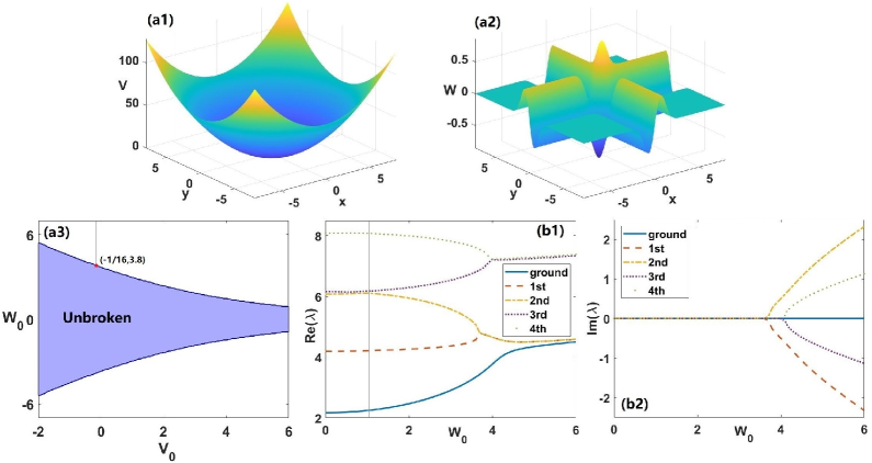
Figure 1: (a1,a2) Real and imaginary parts of the 2D $\mathcal{PT}$-HOG potential (15) with $(V_{0},V_{1},W_{0})=(-1/16,1,1)$. (a3) The blue (white) shaded area shows the area of unbroken (broken) $\mathcal{PT}$ symmetry, as produced by the numerical solution of the linear spectral problem (16) with the $\mathcal{PT}$-HOG potential (15) as $V_{1}=1$. (b1,b2) Real and imaginary parts of the lowest energy eigenvalues $\lambda$ as functions of $W_{0}$ at fixed $V_{0}=-1/16$ and $V_{1}=1$.

3.2 2D nonspinning QDs and their stability in the $\mathcal{PT}$-symmetric potential

In this subsection, we first exhibit exact nonlinear modes for Eq. (11) with $\omega=0$ (without rotation) in the presence of the $\mathcal{PT}$-HOG potential (15). Then, we numerically produce families of generic solutions for the QDs, which include the particular analytical solutions. These are multipolar droplets at low norms $N$ and vortex ones at large $N$. Their stability is investigated in detail.

3.2.1 Exact solutions for 2D nonspinning QDs

2D stationary QDs.—Equation (11) with the chemical potential $\mu=2$ and $\omega=0$ admits the following exact solution, with a nontrivial phase structure, while the local density is the same as in the ground state of the 2D linear Schrödinger equation with the HO potential (i.e., $|\phi(\mathbf{r})|^{2}=\exp(-r^{2})$):

$$\phi(\mathbf{r})\!=\!\exp\!\left\{-\frac{r^{2}}{2}-\frac{i\sqrt{\pi}W_{0}}{8}\left[\mathrm{erf}\left(\frac{x}{2}\right)+\mathrm{erf}\left(\frac{y}{2}\right)\right]\right\},$$ (17)

where the standard error function is defined as $\mathrm{erf}(x)=(2/\sqrt{\pi})\int_{0}^{x}e^{-\eta^{2}}\mathrm{d}\eta$, the norm (8) of the solution being, obviously, $N=\pi$. The solution is a nongeneric one, as it is valid only if parameters $V_{0,1}$ of the real part of potential (15) and nonlinearity coefficient $\sigma$ in Eq. (11) are related by the following constraints:

$$V_{0}=-W_{0}^{2}/16,\qquad V_{1}=\sigma.$$ (18)

In particular, when the imaginary part absents in the $\mathcal{PT}$-HOG potential, i.e., $W_{0}=0$, Eq. (18) demonstrates that the complex $\mathcal{PT}$-HOG potential (15) reduces to the real form,

$$V(\mathbf{r})=r^{2}\left[1+\sigma\exp(-r^{2})\right],$$ (19)

and the corresponding exact solution (17) is identical to the above-mentioned ground-state wave function of the 2D linear Schrödinger equation with the usual HO potential, $\phi(\mathbf{r})=\exp\left(-r^{2}/2\right)$.

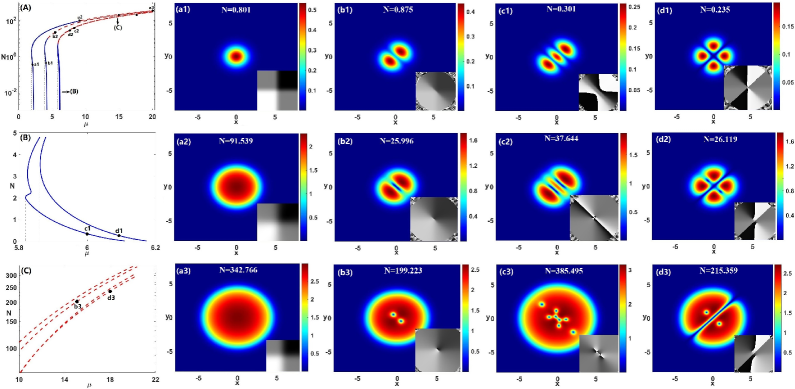
Figure 2: (A) The dependence of norm $N$ on chemical potential $\mu$ for different families of droplet modes, as produced by the full nonlinear equation (9) with $\omega=0$ and $\sigma=1$ (dashed: unstable; solid: stable). (B,C) Zooms of the corresponding locations in (A). Points a1, a2, a3, b1,b2, b3, c1, c2, c3, d1, d2, d3 correspond to examples of QD modes displayed in panels (a1)-(d3). The density and phase structure of one-component QDs: (a1) $\mu=2$, (a2) $\mu=9$, and (a3)$\mu=20$. They correspond, respectively, to points a1, a2, and a3 in Fig. 2(A). Examples of two-component QDs: (b1) $\mu=4$, (b2) $\mu=5.75$, and (b3) $\mu=15$. They correspond, respectively, to points b1, b2, and b3 in Figs. 2(A,C). Examples of three-component QDs: (c1) $\mu=6$, (c2) $\mu=8.2$, and (c3) $\mu=25$. They correspond, respectively, to points c1, c2, and c3 in Figs. 2(A,B). Examples of four-component QDs: (d1) $\mu=6.1$, (d2) $\mu=7.5$, and (d3) $\mu=18$. They correspond, respectively, to points d1, d2, and d3 in Figs. 2(A,B,C). Values of norm $N$ are indicated in each panel.

3.2.2 Numerical solutions for stationary QDs and their stability

The exact solution (17) being available only under constraint (18) makes it necessary to find a family of generic solutions for trapped states in a numerical form. To this end, Eq. (11) with $\omega=0$ was solved by means of the Newton-conjugate-gradient method.

First, we aim to find solutions of the linearized equation (11) with $\sigma=0$, as nonlinear states bifurcate from the linear modes. In particular, we produce the results for parameters

$$W_{0}=1,\qquad V_{0}=-1/16,$$ (20)

which corresponds to the first relation in constraint (18), and may adequately represent the generic case.

The linear spectra produced by the linearized equation (11) with $V_{0}=-1/16$, fixed as per Eq. (20) and varying strength of the strength of the imaginary part of the potential are displayed in Fig. 1(b1). In particular, at $W_{0}=1$, taken as per Eq. (20), the first four eigenvalues are $\lambda_{0}=2.2473,~{}\lambda_{1}=4.216,~{}\lambda_{2}=6.1097,~{}\lambda_{3}=6.1739$, the spectra being pure real.

Droplets with the one-component structure.—$\mathcal{PT}$-symmetric droplets with the simplest structure originate from the above-mentioned linear mode at $\lambda_{0}=2.2473$ with topological charge $m=0$. The dependence between the norm and chemical potential $\mu$ for this solution family is displayed by the leftmost curve in Fig. 2(A). It is seen that the family exists at $\mu>1.9485$. At this point, two different half-branches connect, the bottom and top ones. Their stability is investigated by means of the numerical solutions of the eigenvalue problem based on Eq. (13). The solid blue and dashed red solid segments of the $N(\mu)$ curves represent stable and unstable QD states, respectively.

Examples of the densities and phase structures of QDs of the present types are shown in Fig. 2(a1) for $\mu=2$ (a stable solution marked a1 on the bottom branch in Fig. 2(A)), Fig. 2(a2) for $\mu=9$ (a solution marked a2 on the top branch in Fig. 2(A), where it is located at the stability boundary), and Fig. 2(a3) for $\mu=20$ (an unstable solution marked a3 on the top branch in Fig. 2(A)). Note that the two latter modes feature a flat-top shape with a nearly uniform density in the inner zone.

Droplets with the two-component structure.—Dipole $\mathcal{PT}$-symmetric QDs composed of two separated fragments bifurcate from the above-mentioned linear mode at $\lambda_{1}=4.216$, which represents the first excited state of the linearized equation (11). The phase structure of these modes reveals that it carries topological charge $m=1$. The respective QD family is represented by the middle curve in Fig. 2(A)), which exists at $\mu\geq 3.90054$. At this point, similar to the single-component QD family, the present one is composed of two half-branches connecting at $\mu=3.90054$. An example of the density and phase structure produced by the numerical solution for the stable two-component QD at $\mu=4$ (it corresponds to point b1 in Fig. 2(A)), is shown in Fig. 2(b1). With the increase of the norm the two QD components attract each other and gradually merge into vortex dipoles, as shown in Fig. 2(b2) for $\mu=5.75$. At still larger values of $N$, the two components fuse into a single vortex dipole carried by the flat-top background, with a phase singularity at the center, as shown for $\mu=15$ in Fig. 2(b3).

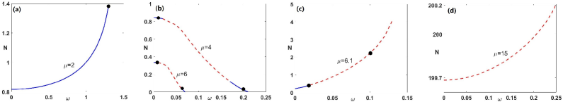
Figure 3: $N(\omega)$ curves for droplets at different values of $\mu$ (dashed: unstable; solid: stable). (a) One-component droplets at $\mu=2$, belonging to the bottom branch in Fig. 2(A). (b) Two- and three-component droplets at $\mu=4$ and $\mu=6$, respectively (they belong to the bottom branch in Fig. 2(A)). (c) Four-components droplets at $\mu=6.1$, belonging to the bottom branch in Fig. 2(A). (d) Two-component droplets at $\mu=15$, belonging to the top branch in Fig. 2(A).

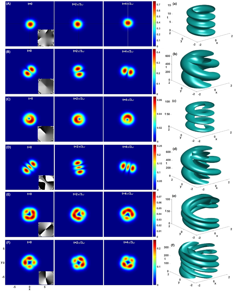
Figure 4: Stable evolution of spinning asymmetric QDs, displayed by means of density isosurfaces in the domain of $|x|,|\,y|\leq 8$. (A) A one-component droplet at $\mu=2$, $\omega=1.35$. (B,C) Two-component droplets at $\mu=4$, with $\omega=0.01$ and $0.2$, respectively. (D,E) Three-component droplets at $\mu=6$, with $\omega=0.01$ and $0.06$, respectively. (F) A four-component droplet at $\mu=6.1$, $\omega=0.02$. (a-f) The corresponding isosurface evolutions with the value of the contour lines taken as the level of $(1/2)\max(|\phi(\mathbf{r})|^{2})$.

Droplets with the three- and four-component structures.—$\mathcal{PT}$-symmetric QDs composed of three separated fragments originate from the above-mentioned mode at $\lambda_{2}=6.1097$ which corresponds to the second excited state of the linearized equation (11). The respective QD family is represented by the rightmost curve $N(\mu)$ in Fig. 2(A), which exists at $\mu\geq 5.8187$. An example of the density and phase structure produced by the numerical solution for the stable two-component QD at $\mu=4$ (it corresponds to point c1 in Fig. 2(B)), is shown in Fig. 2(c1) for $\mu=6$, whose phase structure reveals that it carries topological charge $m=4$. The increase of $N$ leads, as well as in the case of two-component modes, to gradual attraction of the components, as shown for $\mu=8.2$ in Fig. 2(c2), meanwhile the phase structure shows that the topological charge becomes $m=2$. At still larger values of $N$, such as the one corresponding to $\mu=25$ in Fig. 2(c3), the three components fuse into a vortex octupole.

$\mathcal{PT}$-symmetric QDs composed of four separated fragments originate from the above-mentioned mode at $\lambda_{3}=6.1739$, which corresponds to the third excited state of the linearized equation (11). The respective QD family is represented by the curve $N(\mu)$ in Fig. 2(b3) labeled by points d1, d2, and d3. It exists at $\mu\geq 5.8622$. Although this curve is close to the one representing the two-component QDs, the two curves do not intersect (see Fig. 2(B)). An example of the density and phase structure produced by the numerical solution for the stable three-component QD at $\mu=6.1$ (it corresponds to point d1 in Fig. 2(B)), is shown in Fig. 2(d1), whose phase structure implies that it carries topological charge $m=6$. The increase of $N$ again leads to attraction between the components, as shown for $\mu=7.5$ in Fig. 2(d2), which is shaped as a quadrupole droplet. At still larger values of $N$, such as the one corresponding to $\mu=18$ in Fig. 2(d3), the four components fuse pairwise to form a vortex dipole containing two vortices and a phase at the center. The two remaining separate components observed in the latter figure do not fuse with further increase of $N$.

It may be relevant to consider additional species of $\mathcal{PT}$-symmetric QD modes which bifurcate from higher-order excited states of the linearized equation (11). This option will be elaborated elsewhere.

4 2D spinning QDs and their stability

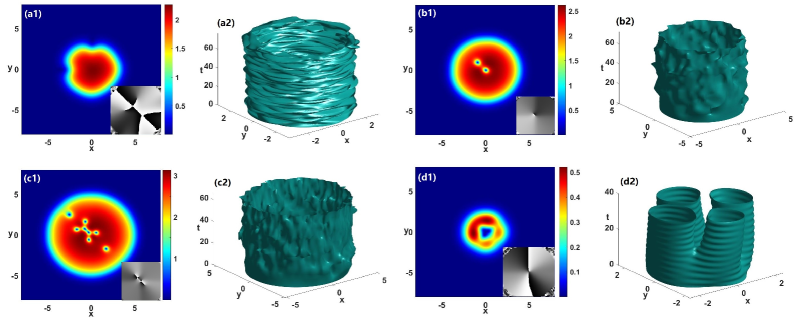
Figure 5: Instable evolutions of spinning asymmetric QDs displayed by means of density isosurfaces. (a1,a2) A one-component droplet at $\mu=9$, $\omega=0.873$. (b1,b2) A two-component droplet at $\mu=15$, $\omega=0.25$. (c1,c2) A three-component droplet at $\mu=25$, $\omega=0.1$. (d1,d2) A four-component droplet at $\mu=6.1$, $\omega=0.1$.

In this section, we address QD modes produced by Eq. (11), which includes the spinning term with $\omega>0$. A family of symmetrically shaped spinning QD solutions of the one-component type is characterized by dependence $N(\omega)$ for a fixed chemical potential. For $\mu=2$, which corresponds, at $\omega=0$, to the bottom branch of the $N(\mu)$ dependence in Fig. 2(A), the $N(\omega)$ curve is displayed in Fig. 3(a). It is seen that the QD’s norm monotonously increases with the increase of the rotation frequency $\omega$. At $\omega\approx 1.35$, the symmetric QD transforms into a slightly asymmetric spinning one, and phase singularities originated from transverse boundary and longitudinal boundary and gradually become larger, see Fig. 4(A). And it is shown that the droplet drifts off the center. Further increase of $\omega$ leads to disappearance of spinning droplets at the critical value $\omega\approx 1.352$, but they remain stable as long as they exist. For example, for $\omega=1.35$, stable rotation of the asymmetric droplet and contour plots for the intensity, taken as the level of $(1/2)\max(|\phi(\mathbf{r})|^{2})$, are exhibited in Figs. 4(A,a). Symmetric QDs belonging to the unstable segment of the $N(\mu)$ curve in Fig. 2(A), such as one with $\mu=9$ (see Fig. 2(a2)) spontaneously transforms into an asymmetric one, which is displayed in Fig. 5(a1). However, the latter state turns out to be unstable, as its norm is too large ($N\approx 91.53$), as shown in Fig. 5(a2).

For QDs with a more sophisticated structure, which includes several components, the dependences $N(\omega)$ for the modes with $\mu=4$ and $\mu=6$, belonging to the bottom branch in Fig. 2(A), are displayed in Fig. 3(b). At a critical value of $\omega$, the norm drops to zero, signaling that the QD disappears at this point. In particular, at $\omega=0.01$ the two components start to fuse and the phase changes, see Fig. 4(B). At $\omega=0.17$, the two components are completely fused into an asymmetric spinning droplet, as seen in Fig. 4(C). However, the spinning QDs are unstable in the region of $0.01<\omega\leq 0.17)$. Similarly, a three-component QD with $\mu=6$ tend to fuse, following the increase of $\omega$. However, as shown in Fig. 4(E), a novel QD appears with four-density peaks at $\omega=0.06$, which is a mode connecting different states. In the regions $[0\leq\omega\leq 0.01]$ and $[0.06\leq\omega\leq 0.07]$ the spinning droplets are stable (see Figs. 4(D,d,E,e)). However, vortex QDs belonging to the top branch in Fig. 2(A) are, generally, unstable. For example, the $N(\omega)$ curve for $\mu=15$ is displayed in Fig. 3(d). In Fig. 5(b2), the rotation drives the two vortices to the top left in the form of a vortex dipole at $\mu=15$, $\omega=0.25$. Similarly, in Figs. 5(c1,c2), for $\omega=0.1$, $\mu=25$ the vortices form an unstable vortex octupole.

For symmetric four-component QDs, the $N(\omega)$ dependence for $\mu=6.1$, belonging to the bottom branch in Fig. 2(A), is displayed in Fig. 3(c). In this case, the dependence is a monotonously growing one, switching from stability to instability. For instance, at $\omega=0.02$, the four components start to fuse pairwise, and the density grows in two of them, as shown in Fig. 4(F). The QDs become unstable with the further increase of $\omega$, see Figs. 5(d1,d2).

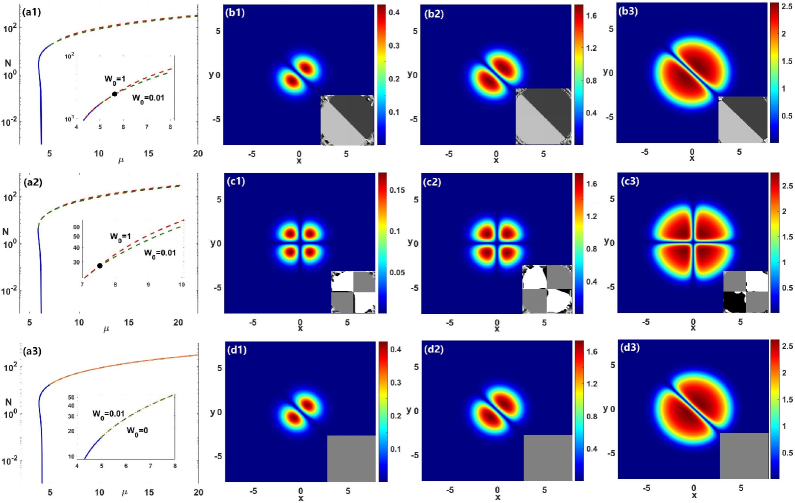
Figure 6: (a1) Dependences of norm $N$ on chemical potential $\mu$ for two-component nonspinning ($\omega=0$) QDs at $W_{0}=1$ and $W_{0}=0.01$. (a2) Dependences of $N$ on chemical potential $\mu$ for four-component QDs at $W_{0}=1$ and $W_{0}=0.01$. (a3) Dependences of norm $N$ on chemical potential $\mu$ for two-component QDs at $W_{0}=0$ and $W_{0}=0.01$ (dashed: unstable; solid: stable). Dipole droplets at $W_{0}=0.01$: (b1) $\mu=4$, (b2) $\mu=5.75$, (b3) $\mu=15$. Quadrupole droplets at $W_{0}=0.01$: (c1) $\mu=6.1$, (c2) $\mu=7.5$, (c3) $\mu=18$. Dipole droplets at $W_{0}=0$ (real potential): (d1) $\mu=4$, (d2) $\mu=5.75$, (d3) $\mu=15$.

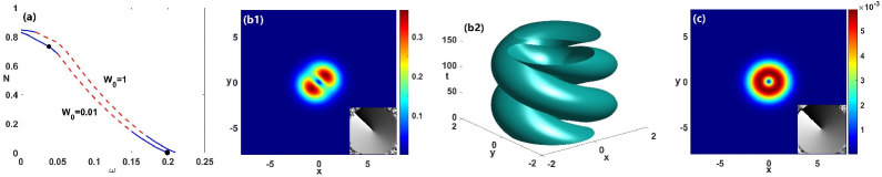
Figure 7: (a) $N(\omega)$ curves for QDs with $\mu=4$ and $W_{0}=1$ or $W_{0}=0.01$ (dashed: unstable; solid: stable). (b1,b2) The evolution of a spinning droplet at $\omega=0.04$ is displayed by means of the density isosurface. (c) A spinning droplet at $\omega=0.2$.

5 Effect of $\mathcal{PT}$-symmetric potential on the (non)spinning QDs

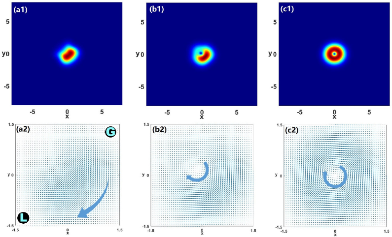
Figure 8: The absolute value $|\vec{S}|$ of the Poynting vector and power flow at $\mu=4$: (a1,a2) $W_{0}=1$, $\omega=0.01$, with points $\mathrm{G}$ and $\mathrm{L}$ points denoting regions where the gain and loss are concentrated, as per Eq. (15). (b1,b2) $W_{0}=1$, $\omega=0.2$; (c1,c2) $W_{0}=0.01$, $\omega=0.04$.

To explore the effect of $\mathcal{PT}$-symmetric potential (15) on the (non)spinning QDs, we vary the strength, $W_{0}$, of gain-loss distribution (imaginary part of the potential).

5.1 The nonspinning case

For the nonspinning case, fixing other potential parameters, $V_{0}$ and $V_{1}$, for QDs with two components we compare dependencies of norm $N$ on chemical potential $\mu$ for $W_{0}=1$ and $W_{0}=0.01$ in Fig. 6(a1). As $\mu\prec 5.75$, The norms $N$ are little affected by gain-loss distribution $W(\mathbf{r})$ (see, for example, Fig. 2(b1) at $W_{0}=1$ and Fig. 6(b1) at $W_{0}=0.01$ for $\mu=4<5.75$). However at $\mu\succeq 5.75$ the QD’s two components start to fuse at $W_{0}=1$ (see Fig. 2(b2)), while for $W_{0}=0.01$ the components of the dipole QD are still well separated, and it remains broad, see Figs. 6(b2, b3). To clarify the role of the $\mathcal{PT}$-symmetric potential, we further change the strength, $W_{0}$, of the gain-loss distribution. For QDs with two components, the dependencies of norm $N$ on chemical potential $\mu$ for $W_{0}=0.01$ and $W_{0}=0$ (the real potential) are shown in Fig. 6(a3). It can be seen that the curves corresponding to $W_{0}=0.01$ and $0$ are virtually identical. Profiles of droplets at $W_{0}=0.01,0$ are almost the same for equal values of chemical potential $\mu$ by comparing Figs. 6(b1-b3) for $W_{0}=0.01$ and Figs. 6(d1-d3) for $W_{0}=0$, respectively. Similarly, for four-component QDs the curves corresponding to $W_{0}=1$ and $0.01$ are nearly identical at small values of $N$ (i.e., at $\mu\prec 7.5$) (see, for example, Fig. 6(a2), and compare Fig. 2(d1) at $W_{0}=1$ and Fig. 6(c1) at $W_{0}=0.01$ for $\mu=6.1<7.5$). However, at larger $N$ (i.e., at $\mu\succeq 7.5$) the two curves split apart, see Fig. 6(a2). For $W_{0}=1$, the four-component QDs start to fuse in pairs (see Figs. 2(d2, d3)), while each component gets broader for $W_{0}=0.01$, see Figs. 6(c2,c3).

5.2 The spinning case

In the spinning regime ($\omega>0$), the gain-loss distribution $W(\mathbf{r})$ affects the symmetry of the droplets. For example, $N(\omega)$ curves for QDs with $\mu=4$ at $W_{0}=1$ and $W_{0}=0.01$ are displayed in Fig. 7(a). With the increase of $\omega$, the norm of the two QD families drops to zero. As shown above, at $W_{0}=1$ the two QD components start to fuse, ending up by forming an asymmetric droplet in Figs. 4(B,C). However, when the strength of the gain-loss distribution is small, the two QD components begin to merge symmetrically, eventually forming a symmetric vortex droplet in Figs. 7(b1,c)). They are stable in the regions $0\leq\omega\leq 0.05$ and $0.15\leq\omega\leq 0.2$.

Due to the presence of the imaginary part of the potential, QDs are amplified (absorbed) in gain (loss) regions. To outline the structure of the nonlinear modes, we use the Poynting vector, which determines the density of the power flow from gain to loss:

$$\begin{array}[]{rl}\vec{S}(x,y)=\frac{i}{2}(\phi\nabla\phi^{\ast}-\phi^{\ast}\nabla\phi),&\end{array}$$ (21)

where $\phi$ is the nonlinear localized mode produced by Eq. (11). In the nonspinning regime, the power always flows from the gain to the loss. As the angular velocity $\omega$ increases, the direction of the power flow shifts, and then a vortex is formed, as seen in Figs. 8(a1,a2,b1,b2). The strong gain-loss distribution makes the QDs become asymmetric, see Figs. 4(B,C). On the other hand, if the gain-loss term is weak with small $W_{0}$, the effect of the rotation on the energy flow is dominant. Therefore, in that case the energy flow supports symmetric QDs, see Figs. 8(c1,c2).

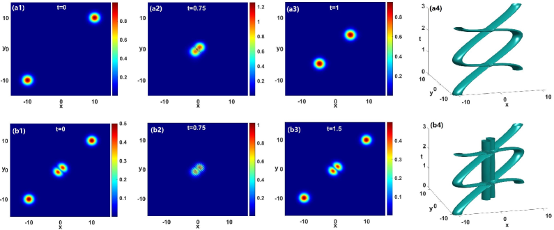
Figure 9: (a1-a4) The collision of two nonspinning droplets (with $A=1$ and $B=0$ in Eq. (22)) at different times, and the respective isosurface evolution. (b1-b4) The collision of two nonspinning droplets (with $A=0.5$ and $B=1$) at different times and the respective isosurface evolution, where $\phi(\mathbf{r})$ in Eq. (22) is the dipole droplet at $\mu=4$. The strength of the gain-loss distribution is $W_{0}=1$.

6 Interactions between spinning or nonspinning QDs

For collisions between two or three QDs, we address changes of the state of spinning or nonspinning droplets produced by the collisions. The corresponding initial condition is taken as a superposition of separated droplets:

$$\psi(\mathbf{r},t=0)=A[\phi_{1}(\mathbf{r}-\mathbf{r}_{0})+\phi_{1}(\mathbf{r}+\mathbf{r}_{0})]+B\phi(\mathbf{r}),$$ (22)

where $\phi_{1}(\mathbf{r})$ is the exact QD solution given by Eq. (17), and $\phi(\mathbf{r})$ may be an additional solution of stationary equation (11). Parameters $\mathbf{r}_{0}=(x_{0},y_{0})$ define initial positions of the colliding QDs, and coefficients $A$ and $B$ determine the composition of the input.

The real part of potential (15) draws the QDs towards the center and leads to the collision. First, we consider the collision of a pair of nonspinning droplets ($\omega=0$), which corresponds to $A=1$ and $B=0$ in Eq. (22). Figures 9(a1, a3, a4) demonstrate an elastic collision, which preserves shapes of both droplets. At the collision point, at $t=0.75$, an interference pattern appears, which is a distinctive feature of the interplay of coherent matter waves, as seen in Fig. 9(a2). For the collision of two spinning QDs, for example, $\omega=1$, Figure 10(a1) demonstrates an elastic collision between two spinning QDs, by means of the density isosurface taken at $(1/2)\max(|\phi(\mathbf{r})|^{2})$. Figure 10(a2) additionally shows the evolution of the isosurface in projection onto the $\left(x,y\right)$ plane in the course of the rotation period $2\pi/\omega$. This plot shows that $\phi_{1}(\mathbf{r}+\mathbf{r}_{0})$ follows trajectory $(1)\rightarrow(2)\rightarrow(3)\rightarrow(2)\rightarrow(4)\rightarrow(2)\rightarrow(5)\rightarrow(2)\rightarrow(1)$, finally returning to the initial position.

For the collision of three nonspinning droplets in Eq. (22) corresponding to $\mu=4$, with $A=0.5$ and $B=1$, where $\phi(\mathbf{r})$ is the respective dipole droplet, the collision remains perfectly elastic, with the interference pattern appearing in the course of the collision, see Figs. 9(b1)-(b4). For the collision of thee spinning QDs, for example, $\omega=0.2$, Fig. 10(b1) also demonstrates an elastic collision between three spinning QDs, by means of the density isosurface taken at $(1/2)\max(|\phi(\mathbf{r})|^{2})$. The interaction seems to be complicated (see Fig. 10(b2) for the projection of the isosurface onto the $\left(x,y\right)$ plane).

These results indicate that collisions between 2D $\mathcal{PT}$-symmetric spinning or nonspinning QDs are similar to what is known about other nonintegrable models, such the one for one-dimensional QDs [21, 62].

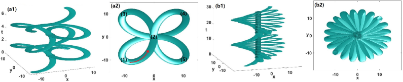
Figure 10: (a1) The isosurface evolution for the collision of two spinning droplets with $\omega=1$, and (a2) its projection onto the $\left({\small x,y}\right)$ plane, corresponding to nonspinning ones in Fig. 9(a4). (b1) The isosurface evolution for the collision of three spinning droplets with $\omega=0.2$, and its projection onto the $\left({\small x,y}\right)$ plane, corresponding to nonspinning ones in Fig. 9 (b4). The strength of the gain-loss distribution is $W_{0}=1$.

7 Conclusions and discussions

We have introduced the 2D dynamical model for the BEC under the action of the $\mathcal{PT}$-symmetric potential, including the LHY correction. The linear spectrum of the model remains real up to a critical strength of the imaginary part of the potential. In the region of the unbroken $\mathcal{PT}$ symmetry, several families of QDs (quantum droplets) originating from the linear modes are obtained, in the form of multipolar modes with smaller norms, and vortex ones with larger norms. A particular solution is obtained in the exact analytical form. Stability of these QD states is explored by means of numerical methods. The effect of the rotation (spinning) on the QDs is studied too, showing that the asymmetric energy flow, resulting from the imbalance of the gain-loss distribution and rotation, creates asymmetric spinning QDs. Collisions between spinning QDs are explored too, with a conclusion that they tend to be elastic.

The analysis presented in this paper can be extended for solitons, including spinning ones, in models combining the nonlinearity and $\mathcal{PT}$ symmetry with fractional diffraction, cf. Refs. [68, 69].

Acknowledgments

The work was supported by the National Natural Science Foundation of China (No. 11925108) and Israel Science Foundation (No. 1695/2022).

References

- [1] D. S. Petrov, Quantum mechanical stabilization of a collapsing Bose-Bose mixture, Phys. Rev. Lett. 115, 155302 (2015).
- [2] D. S. Petrov and G. E. Astrakharchik, Ultradilute low-dimensional liquids, Phys. Rev. Lett. 117, 100401 (2016).
- [3] T. D. Lee, K. Huang, and C. N. Yang, Eigenvalues and eigenfunctions of a Bose system of hard spheres and its low-temperature properties, Phys. Rev. 106, 1135 (1957).
- [4] A. Bulgac, Dilute quantum droplets, Phys. Rev. Lett. 89, 050402 (2002).
- [5] L. Chomaz, S. Baier, D. Petter, M. J. Mark, F. Wachtler, L. Santos, and F. Ferlaino, Quantum-fluctuation-driven crossover from a dilute Bose-Einstein condensate to a macrodroplet in a dipolar quantum fluid, Phys. Rev. X 6, 041039 (2016).
- [6] D. Edler, C. Mishra, F. Wächtler, R. Nath, S. Sinha, and L. Santos, Quantum fluctuations in quasi-one-dimensional dipolar Bose-Einstein condensates. Phys. Rev. Lett. 119, 050403 (2017).
- [7] F. Böttcher, J.-N. Schmidt, J. Hertkorn, K. S. H. Ng, S. D. Graham, M. Guo, T. Langen, and T. Pfau, New states of matter with fine-tuned interactions: quantum droplets and dipolar supersolids, Rep. Prog. Phys. 84, 012403 (2021).
- [8] Z. H. Luo, W. Pang, B. Liu, Y. Y. Li, and B. A. Malomed, A new form of liquid matter: Quantum droplets, Front. Phys. 16, 32201 (2021).
- [9] B. A. Malomed, Multidimensional Solitons (American Institute of Physics Publishers: Melville, NY, 2022).
- [10] V. Cikojevć, K. Dzelalija, P. Stipanović, L. V. Markić, and J. Boronat, Ultradilute quantum liquid drops, Phys. Rev. B 97, 140502(R) (2018).
- [11] G. De Rosi, G. E. Astrakharchik, P. Massignan, Thermal instability, evaporation, and thermodynamics of one-dimensional liquids in weakly interacting Bose-Bose mixtures. Phys. Rev. A 103, 043316 (2021).
- [12] I. Ferrier-Barbut, H. Kadau, M. Schmitt, M. Wenzel, and T. Pfau, Observation of quantum droplets in a strongly dipolar Bose gas. Phys. Rev. Lett. 116, 215301 (2016).
- [13] H. Kadau, M. Schmitt, M. Wentzel, C. Wink, T. Maier, I. Ferrier-Barbut, and T. Pfau, Observing the Rosenzweig instability of a quantum ferrofluid, Nature 530, 194 (2016).
- [14] M. Schmitt, M. Wenzel, F. Büttcher, I. Ferrier-Barbut, and T. Pfau, Self-bound droplets of a dilute magnetic quantum liquid, Nature 539, 259 (2016).
- [15] C. Cabrera, L. Tanzi, J. Sanz, B. Naylor, P. Thomas, P. Cheiney, and L. Tarruell, Quantum liquid droplets in a mixture of Bose-Einstein condensates, Science 359, 301 (2018).
- [16] P. Cheiney, C. R. Cabrera, J. Sanz, B. Naylor, L. Tanzi, and L. Tarruell, Bright soliton to quantum droplet transition in a mixture of Bose-Einstein condensates, Phys. Rev. Lett. 120, 135301 (2018).
- [17] G. Semeghini, G. Ferioli, L. Masi, C. Mazzinghi, L. Wolswijk, F. Minardi, M. Modugno, G. Modugno, M. Inguscio, and M. Fattori, Self-bound quantum droplets of atomic mixtures in free space? Phys. Rev. Lett. 120, 235301 (2018).
- [18] G. Ferioli, G. Semeghini, L. Masi, G. Giusti, G. Modugno, M. Inguscio, A. Gallemí, A. Recati, and M. Fattori, Collisions of self-bound quantum droplets, Phys. Rev. Lett. 122, 090401 (2019).
- [19] T. G. Skov, M. G. Skou, N. B. Jørgensen, and J. J. Arlt, Observation of a Lee-Huang-Yang Fluid, Phys. Rev. Lett. 126, 230404 (2021).
- [20] C. D’Errico, A. Burchianti, M. Prevedelli, L. Salasnich, F. Ancilotto, M. Modugno, F. Minardi, and C. Fort, Observation of quantum droplets in a heteronuclear bosonic mixture, Phys. Rev. Research 1, 033155 (2019).
- [21] G. E. Astrakharchik and B. A. Malomed, Dynamics of one-dimensional quantum droplets, Phys. Rev. A 98, 013631 (2018).
- [22] M. Tylutki, G. E. Astrakharchik, B. A. Malomed, and D. S. Petrov, Collective excitations of a one-dimensional quantum droplet, Phys. Rev. A 101, 051601(R) (2020).
- [23] F. K. Abdullaev, A. Gammal, R. K. Kumar, and L. Tomio, Faraday waves and droplets in quasi-one-dimensional Bose gas mixtures, J. Phys. B 52, 195301 (2019).
- [24] S. R. Otajonov, E. N. Tsoy, and F. K. Abdullaev, Stationary and dynamical properties of one-dimensional quantum droplets, Phys. Lett. A 383, 125980 (2019).
- [25] Y. Li, Z. Chen, Z. Luo, C. Huang, H. Tan, W. Pang, and B. A. Malomed, Two-dimensional vortex quantum droplets, Phys. Rev. A 98, 063602 (2018).
- [26] Y. V. Kartashov, B. A. Malomed, and L. Torner, Metastability of quantum droplet clusters, Phys. Rev. Lett. 122, 193902 (2019).
- [27] E. Shamriz, Z. Chen, and B. A. Malomed, Suppression of the quasi-two-dimensional quantum collapse in the attraction field by the Lee-Huang-Yang effect, Phys. Rev. A 101, 063628 (2020).
- [28] Y. V. Kartashov, B. A. Malomed, L. Tarruell, and L. Torner, Three-dimensional droplets of swirling superfluids, Phys. Rev. A 98, 013612 (2018).
- [29] A. Cidrim, F. E. A. dos Santos, E. A. L. Henn, and T. Macrí, Vortices in self-bound dipolar droplets, Phys. Rev. A 98, 023618 (2018).
- [30] V. I. Yukalov, A. N. Novikov, V. S. Bagnato, Formation of granular structures in trapped Bose-Einstein condensates under oscillatory excitations. Laser Phys. Lett. 11, 095501 (2014).
- [31] L. Dong, D. Liu, Z. Du, K. Shi, W. Qi, Bistable multipole quantum droplets in binary Bose-Einstein condensates, Phys. Rev. A 105, 033321 (2022).
- [32] Y. V. Kartashov, V. M. Lashkin, and M. Modugno, L. Torner, Spinor-induced instability of kinks, holes and quantum droplets, New J. Phys. 24, 073012 (2022).
- [33] S. R. Otajonov, E. N. Tsoy, F. K. Abdullaev, Modulational instability and quantum droplets in a two-dimensional Bose-Einstein condensate, Phys. Rev. A 106, 033309 (2022).
- [34] S. M. Roccuzzo, A. Gallemí, A. Recati, and S. Stringari, Rotating a supersolid dipolar gas, Phys. Rev. Lett. 124, 045702 (2020).
- [35] L. Dong, K. Shi, and C. Huang, Internal modes of two-dimensional quantum droplets, Phys. Rev. A 106, 053303 (2022).
- [36] T. Mithun, A. Maluckov, K. Kasamatsu, B. Malomed, and A. Khare, Inter-component asymmetry and formation of quantum droplets in quasi-one-dimensional binary Bose gases, Symmetry 12, 174 (2020).
- [37] X. Zhang, X. Xu, Y. Zheng, Z. Chen, B. Liu, C. Huang, B. A. Malomed, and Y. Li, Semidiscrete Quantum Droplets and Vortices, Phys. Rev. Lett. 123, 133901 (2019).
- [38] M. R. Pathak, A. Nath, Dynamics of quantum droplets in an external harmonic confinement, Sci. Rep. 12, 6904 (2022).
- [39] L. Dong and Y. V. Kartashov, Rotating multidimensional quantum droplets, Phys. Rev. Lett. 126, 244101 (2021).
- [40] H. Hu and X. J. Liu, Collective excitations of a spherical ultradilute quantum droplet, Phys. Rev. A 102, 053303 (2020).
- [41] Y. Y. Zheng, S. T. Chen, Z. P. Huang, S. X. Dai, B. Liu, Y. Y. Li, and S. R. Wang, Quantum droplets in two-dimensional optical lattices, Front. Phys. 16, 22501 (2021).
- [42] C. M. Bender and S. Boettcher, Real spectra in non-Hermitian Hamiltonians having symmetry, Phys. Rev. Lett. 80, 5243 (1998).
- [43] Z. Yan, Z. Wen, and V. V. Konotop, Solitons in a nonlinear Schrödinger equation with -symmetric potentials and inhomogeneous nonlinearity: Stability and excitation of nonlinear modes, Phys. Rev. A 92, 023821 (2015).
- [44] Z. H. Musslimani, K. G. Makris, R. E. Ganainy, and D. N. Christodoulides, Analytical solutions to a class of nonlinear Schrödinger equations with -like potentials, J. Phys. A 41, 244019 (2008).
- [45] S. Hu, X. Ma, D. Lu, Z. Yang, Y. Zheng, and W. Hu, Solitons supported by complex -symmetric Gaussian potentials, Phys. Rev. A 84, 043818 (2011).
- [46] V. Achilleos, P. Kevrekidis, D. Frantzeskakis, and R. Carretero-Gonzalez, Dark solitons and vortices in -symmetric nonlinear media: From spontaneous symmetry breaking to nonlinear phase transitions, Phys. Rev. A 86, 013808 (2012).
- [47] C. Dai, X. Wang, and G. Zhou, Stable light-bullet solutions in the harmonic and parity-time-symmetric potentials, Phys. Rev. A 89, 013834 (2014).
- [48] M. Znojil, Quantum phase transitions in nonhermitian harmonic oscillator, Sci. Rep. 10, 1 (2020).
- [49] D. A. Zezyulin and V. V. Konotop, Nonlinear modes in the harmonic -symmetric potential, Phys. Rev. A 85, 043840 (2012).
- [50] V. V. Konotop, J. Yang, and D. A. Zezyulin, Nonlinear waves in -symmetric systems, Rev. Mod. Phys. 88, 035002 (2016).
- [51] A. Guo, G. Salamo, D. Duchesne, R. Morandotti, M. Volatier-Ravat, V. Aimez, G. Siviloglou, and D. N. Christodoulides, Observation of -symmetry breaking in complex optical potentials, Phys. Rev. Lett. 103, 093902 (2009).
- [52] C. E. Rüter, K. G. Makris, R. El-Ganainy, D. N. Christodoulides, M. Segev, and D. Kip, Observation of parity-time symmetry in optics, Nat. Phys. 6, 192-195 (2010).
- [53] K. G. Makris, R. El-Ganainy, D. N. Christodoulides, and Z. H. Musslimani, Beam dynamics in symmetric optical lattices, Phys. Rev. Lett. 100, 103904 (2008).
- [54] A. L. M. Muniz, M. Wimmer, A. Bisianov, U. Peschel, R. Morandotti, P. S. Jung, and D. N. Christodoulides, 2D Solitons in -Symmetric Photonic Lattices, Phys. Rev. Lett. 123, 253903 (2019).
- [55] H. Cartarius and G. Wunner, Model of a -symmetric Bose-Einstein condensate in a delta-function double-well potential, Phys. Rev. A 86, 013612 (2012).
- [56] M. Kreibich, J. Main, H. Cartarius, and G. Wunner, Tilted optical lattices with defects as realizations of symmetry in Bose-Einstein condensates, Phys. Rev. A 93, 023624 (2016).
- [57] F. Kogel, S. Kotzur, D. Dizdarevic, J. Main, and G. Wunner, Realization of -symmetric and -symmetry broken states in static optical-lattice potentials, Phys. Rev. A 99, 063610 (2019).
- [58] C. Hang, D. A. Zezyulin, G. Huang, V. V. Konotop, and B. A. Malomed, Tunable nonlinear double-core -symmetric waveguides, Opt. Lett. 39, 5387-5390 (2014).
- [59] Z. Zhou, X. Yu, Y. Zou, and H. Zhong, Dynamics of quantum droplets in a one-dimensional optical lattice, Commun. Nonlinear Sci. Numer. Simulat. 78, 104881 (2019).
- [60] B. Liu, H. Zhang, R. Zhong, X. Zhang, X. Qin, C. Huang, Y. Li, and B. A. Malomed, Symmetry breaking of quantum droplets in a dual-core trap, Phys. Rev. A 99, 053602 (2019).
- [61] Z. Zhou, B. Zhu, H. Wang, H. Zhong, Stability and collisions of quantum droplets in -symmetric dual-core couplers, Commun. Nonlinear Sci. Numer. Simulat. 91, 105424 (2020).
- [62] J. Song and Z. Yan, Dynamics of 1D and 3D quantum droplets in parity-time-symmetric harmonic-Gaussian potentials with two competing nonlinearities, Physica D 442, 133527 (2022).
- [63] J. Yang and T. I. Lakoba, Universally-convergent squared-operator iteration methods for solitary waves in general nonlinear wave equations, Stud. Appl. Math. 118, 153-197 (2007).
- [64] J. Yang, Newton-conjugate-gradient methods for solitary wave computations, J. Comput. Phys. 228, 7007-7024 (2009).
- [65] M. J. Ablowitz and Z. H. Musslimani, Spectral renormalization method for computing self-localized solutions to nonlinear systems, Opt. Lett. 30, 2140-2142 (2005).
- [66] J. Yang, Nonlinear Waves in Integrable and Nonintegrable Systems (SIAM, 2010).
- [67] Y. Chen and Z. Yan, Multi-dimensional stable fundamental solitons and excitations in -symmetric harmonic-Gaussian potentials with unbounded gain-and-loss distributions, Commun. Nonlinear Sci. Numer. Simul. 57, 3446 (2018).
- [68] Y. Q. Zhang, H. Zhong, M. R. Belić, Y. Zhu, W. P. Zhong, Y. P. Zhang, D. N. Christodoulides, and M. Xiao, symmetry in a fractional Schrödinger equation, Laser & Photon. Rev. 10, 526-531 (2016).
- [69] X. K. Yao and X. M. Liu, Solitons in the fractional Schrödinger equation with parity-time-symmetric lattice potential, Photonic Research 6, 875-887 (2018).