Fat $b$-Jet Analyses Using Old and New Clustering Algorithms
in New Higgs Boson Searches at the LHC

Abstract

We compare different jet-clustering algorithms in establishing fully hadronic final states stemming from the chain decay of a heavy Higgs state into a pair of the 125 GeV Higgs boson that decays into bottom-antibottom quark pairs. Such $4b$ events typically give rise to boosted topologies, wherein $b\bar{b}$ pairs emerging from each 125 GeV Higgs boson tend to merge into a single, fat $b$-jet. Assuming Large Hadron Collider (LHC) settings, we illustrate how both the efficiency of selecting the multi-jet final state and the ability to reconstruct from it the masses of all Higgs bosons depend on the choice of jet-clustering algorithm and its parameter settings. We indicate the optimal choice of clustering method for the purpose of establishing such a ubiquitous Beyond the SM (BSM) signal, illustrated via a Type-II 2-Higgs Doublet Model (2HDM).

1 Introduction

The Higgs boson discovered in 2012 at the LHC has been extensively studied, so that we now know that it is very SM-like [1]. That is, it is clear that its quantum numbers (charge, spin, CP) are consistent with those predicted in the SM and so are its couplings, at least those measured thus far, to $W^{\pm}$ and $Z$ bosons as well as to $t,b,c,\tau$ and $\mu$ fermions. Amongst of all these, the $Hb\bar{b}$ coupling plays a particular role, for a twofold reason. On the one hand, it is the dominant one for the SM-like Higgs state, as the $b\bar{b}$ decay rate is the largest [2, 3], while also being the one most polluted by large backgrounds (chiefly including the overwhelming $t\bar{t}$ production and decay). On the other hand, the $b\bar{b}$ decay channel presents significant challenges experimentally, primarily connected to the necessity of flavour tagging it amongst myriads of light-quark and gluon jets stemming from the majority of Quantum Chromo-Dynamics (QCD) interactions, apart from $b$-jets from background $t\bar{t}$ decays.

It is therefore important to assess the current status of phenomenological approaches to the extraction of these multi-$b$-jet signals. While there exists copious literature on this topic within the SM, wherein, in the foreseeable future (i.e., Run 3 of the LHC), the SM-like Higgs state can only be produced singly, comparatively less developed are studies of pair production in Beyond the SM (BSM) scenarios, despite significant cross sections for a resonant decay of a heavier Higgs boson leading to the Higgs pair decaying to a $4b$ final state. This is why, in Ref. [5], we studied the process $pp\to H\to hh\to 4b$, for $m_{H}=125$ GeV and $m_{h}$ between 40 and 60 GeV, which would be a striking signal of, for example, a 2-Higgs Doublet Model (2HDM) [6, 7, 8] in the so-called ‘inverted hierarchy’ scenario, i.e., when the discovered Higgs state is not the lightest one.

In that paper, we assessed the ability of different jet-clustering algorithms, with different resolution parameters and reconstruction procedures, to resolve such fully hadronic final states. Therein, we showed that both the efficiency of selecting the hadronic states and the ability to reconstruct Higgs masses from these depend strongly on the choice of the jet-clustering algorithm and its settings. Specifically, we emphasised that variable-$R$ algorithms [9] were more effective in gaining signal sensitivity as well as in reconstructing the light and heavy Higgs mass peaks, than those based on a fixed cone radius $R$ [10, 11].

Those results were obtained for slim $b$-jets, for which no merging occurred (so we looked at typical four $b$-jet configurations). In the present paper, we want to instead study the case of fat $b$-jets, i.e., when two $b$-partons emerging from a $h$ decay are not resolved as individual jets, but are merged into a fat $b$-jet containing both. This is most likely to occur when the $H$ state is significantly heavier than the $h$, $m_{H}\gg m_{h}=125$ in the usual 2HDM in the ‘standard hierarchy’ scenario. Again, we will assess which of the two types of jet-clustering algorithms, fixed or variable cone size, is better able to extract the signal from the backgrounds and yield the sharpest rendition of the Breit-Wigner mass peaks. For this purpose, we will implement a simplified (MC truth informed) double $b$-tagger. It is worthwhile to mention that one can use other boosted jet tagging methods based on the jet substructure technique to further enhance the signal significances, e.g., N-subjettiness variables and their ratios [12], Energy Correlation Functions (ECF) and their ratios [13, 14], or a combination of substructure based observables and cutting edge machine learning techniques [15]. Many experimental studies have been done on the fat jets analysis [16, 17, 18, 19].

The plan of the paper is as follows. In the next section, we describe how jets are defined at the LHC. We then move on to describe the Monte Carlo (MC) analysis that we will perform (i.e., simulation tools, cutflow, $b$-tagger, etc.). After which we will present our results. Finally, in the last section, we will draw our conclusions.

2 Jets at the LHC

In a modern particle collider, such as the LHC, the most crucial difficulty in extracting new physics is making sense out of the mess of particles collected in the detectors in each event. A so-called jet definition provides a mapping between hard interactions in our Quantum Field Theory (QFT), which is what we are ultimately looking to test, and the jumble of particles we actually observe in the detectors.

One of the well-known peculiarities of QCD is colour confinement, i.e., the fact that quarks and gluons cannot exist as free particles, instead only appear inside hadronic bound states. In the high energy environment of the LHC, they undergo showering and hadronisation and are detected as sprays of (colourless) hadrons.

A simple, intuitive picture of this process is to consider the emission rate for a quark(antiquark) to radiate a gluon, given by [20, 21, 22, 23]

$$\mathcal{P}_{gq}(z)=C_{F}\biggr{[}\frac{1+(1-z)^{2}}{z}\biggr{]},$$ (1)

and, similarly, for a gluon radiating another gluon,

$$\mathcal{P}_{gg}(z)= C_{A}\biggr{[}\frac{z}{1-z}+\frac{1-z}{z}+z(1-z)\biggr{]}+$$

$$+\delta(1-z)\frac{(11C_{A}-4n_{f}T_{R})}{6},$$ (2)

Sometimes, a gluon could also split into a quark-antiquark pair, according to

$$\mathcal{P}_{qg}(z)=T_{R}\biggr{[}z^{2}+(1-z)^{2}\biggr{]},$$ (3)

where $z$ and $(1-z)$ are the energy fractions, $n_{f}$ is the number of fermions coupling to the gluons, $C_{F}$, $C_{A}$ and $T_{R}$ are the usual QCD ‘colour factors’.

These splittings repeat themselves in all possible combinations, thereby generating the aforementioned shower, wherein partons are rather soft and/or collinear (note the $E$ and $\theta$ ‘divergences’), so that the final partons are rather collimated in the direction of the primary ones. Once the energy of the initial collision is spread amongst all these subsequent partons so that the average value of it is close to $\Lambda_{\rm QCD}$, the hadronisation process takes place by generating hadrons (pions, kaons, etc.) which directions are also aligned with those of the primary partons (assuming that $Q\gg\Lambda_{\rm QCD}$). (Recall that, owing to the running of the QCD coupling constant, the partonic couplings will reach the non-perturbative regime before partons reach the detectors.) The end result is the creation of the aforementioned sprays of hadrons, called jets. However, no matter how intuitive this qualitative picture is, one needs a quantitative algorithm to define such jets.

2.1 Jet Clustering Algorithms

We here review two classes of jet clustering algorithms currently in use at the LHC.

2.1.1 Fixed Cone Jets

To provide a mapping between hard interactions and the hadronic sprays observed in particle detectors, algorithmic procedures are used to characterise the aforementioned jets. Over the years, there has been extensive development of jet clustering algorithm, beginning in 1977 with Sterman and Weinberg [24], who indeed defined jets as cones, initially deployed in the context of $e^{+}e^{-}\rightarrow$ hadron scatterings. The type of algorithms currently employed at the LHC, and of particular interest for this study, are known as sequential recombination algorithms [25], or ‘jet clustering algorithms’.

Jet clustering algorithms reduce the complexity of final states by attempting to rewind the showering/hadronisation process. They consider each particle in an event and all are iteratively combined together based on some inter-particle distance measure to form jets. Remarkably, when a jet clustering algorithm is well designed, it can be applied at both the parton and hadron levels, so as to enable one to make direct comparisons between theory and experiment.

All (sequential) jet clustering algorithms currently used at the LHC employ a similar method descending from a generalised $k_{T}$ algorithm. This uses an inter-particle distance measure between two particles ($i$ and $j$), given as

$$d_{ij}={\rm min}(p_{Ti}^{2n},p_{Tj}^{2n})\frac{\Delta R^{2}_{ij}}{R^{2}},$$ (4)

where $\Delta R^{2}_{ij}=(y_{i}-y_{j})^{2}+(\phi_{i}-\phi_{j})^{2}$ is an angular distance between two particles $i$ and $j$, with $y$ and $\phi$ being the rapidity and azimuth of the associated final state hadron, $n$ is an exponent corresponding to a particular jet clustering algorithm and $R$ is the jet radius (or cone radius) parameter. The second distance variable is the ‘beam distance’:

$$d_{Bi}=p_{Ti}^{2n},$$ (5)

which is the separation between object $i$ and the beam $B$. The algorithm works by finding the minimum $d_{\rm min}$ of all the $d_{ij}$’s and $d_{Bi}$’s and then the following happens.

• If $d_{\rm min}$ is a $d_{ij}$, combine $i$ and $j$ then repeat the process.

• If $d_{\rm min}$ is a $d_{Bi}$, then $i$ is declared a jet and removed from the list. This procedure is then repeated until no particles are left.

If we now take into account some pair of pseudojets $i$ and $j$, with $i$ having lower $p_{T}$ than $j$ and being selected in $d_{ij}$, we can write (for $n\geq 0$)

$${d_{ij}=\frac{\Delta R^{2}_{ij}}{R^{2}}p^{2n}_{Ti}=\frac{\Delta R^{2}_{ij}}{R^{2}}d_{Bi}.}$$ (6)

For $n\leq 0$, it will be other way around with $p_{Tj}$ selected from $d_{ij}$ and the above equation will change to:

$${d_{ij}=\frac{\Delta R^{2}_{ij}}{R^{2}}p^{2n}_{Tj}=\frac{\Delta R^{2}_{ij}}{R^{2}}d_{Bj}.}$$ (7)

We require the ratio $\frac{\Delta R^{2}_{ij}}{R^{2}}<1$ to evade declaring $i$ a jet instead of combining $i$ with $j$, therefore parameter $R$ acts as a cut-off for the particle pairing and is proportional to the final size of the jets. The algorithms currently most used at the LHC are the anti-$k_{T}$ [10, 11] and the Cambridge/Aachen (C/A) ones [26, 27]. The $n$ value for the anti-$k_{T}$ and C/A algorithms are $-1$ and 0, respectively.

2.1.2 Variable-$\boldmath{R}$ Jets

The fixed input parameter, $R$, mentioned above acts as a cut-off for particle pairing and applying a size limit on the jets based on the separation between the particles. We also know that the angular spread of the jet constituents depends on the initial partons $p_{T}$. For objects with high $p_{T}$, the decay products are more tightly packed into a collimated cone whereas for the objects with lower $p_{T}$, the constituents will be spread over some wider angle. Therefore, it is very important to carefully select the right $R$ value for clustering depending on the relevant $p_{T}$ distribution to capture the underlying physics.

The more recent variation of the standard jet clustering algorithms is the so-called Variable-$R$ jet clustering algorithm [9], which alters the scheme mentioned in Section 2.1.1 to adapt with jets of varying cone size in an event. A modification is made to the distance measure $d_{ij}$, such that:

$$d_{ij}={\rm min}(p_{Ti}^{2n},p_{Tj}^{2n})\Delta R^{2}_{ij}$$ (8)

and

$$d_{Bi}=p_{Ti}^{2n}R^{2}.$$ (9)

Next, the fixed input parameter $R$ is replaced by a $p_{T}$ dependent $R_{\rm eff}(p_{Ti})=\frac{\rho}{p_{T}}$, where $\rho$ is a dimensionful input parameter, such that:

$$d_{Bi}=p_{Ti}^{2n}R_{\rm eff}(p_{Ti})^{2}.$$ (10)

For objects with larger $p_{T}$, $d_{Bi}$ will be suppressed and these objects are more likely to be classified as jets, For objects with lower $p_{T}$, these are combined with the nearest neighbour increasing the spread of constituents as $d_{Bi}$ is more enhanced.

In the variable-$R$ approach, the process is modified in such a way that one can avoid events with very wide jets at low $p_{T}$. The dimensionful parameter $\rho$ can be scanned over a range to optimise the maximum desired sensitivity. This can also be done for other parameters such as $R_{\rm min/max}$ (cut-offs for the minimum and maximum allowed $R_{\text{\rm eff}}$), respectively, i.e., if a jet has $R_{\text{\rm eff}}<R_{\rm min}$, it is overwritten and set to $R_{\text{\rm eff}}=R_{\rm min}$ and equivalently for $R_{\rm max}$.

At last, we hypothesise that using a variable-$R$ clustering procedure can show improvement in reconstructing signal when compared to traditional fixed-$R$ routines. The variable-$R$ technique helps in reducing the complexity of finding a suitable single fixed cone size to envelop all the radiation without including too much outside noise or ’junk’ inside a jet. This will be quite useful for our study as we look at constructing fatjets.

3 Methodology

In this section, we describe the tools and selection strategy to pursue our analysis.

3.1 Simulation Details

We consider a suitable Benchmark Point (BP) in the context of the 2HDM Type-II (2HDM-II henceforth) where we assume the lightest CP-even Higgs state to be the SM-like Higgs Boson with $m_{h}$ = 125 GeV and set the heavier CP-even Higgs boson mass as $m_{H}$ = 700 GeV. The BP has been tested against theoretical and experimental constraints by using 2HDMC [28] interfaced with HiggsBounds [29] and HiggsSignals [30] and against flavour constraints using SuperISO [31]. Specifically, concerning the latter, the following flavour constraints on meson decay Branching Ratios (BRs) and mixings, all to the $2\sigma$ level, are used in our analysis: ${\rm BR}(b\rightarrow s\gamma)$, ${\rm BR}(B_{s}\rightarrow\mu\mu)$, ${\rm BR}(D_{s}\rightarrow\tau\nu)$, ${\rm BR}(D_{s}\rightarrow\mu\nu)$, ${\rm BR}(B_{u}\rightarrow\tau\nu)$, $\frac{{\rm BR}(K\rightarrow\mu\nu)}{{\rm BR}(\pi\rightarrow\mu\nu)}$, ${\rm BR}(B\rightarrow D_{0}\tau\nu)$ and $\Delta_{0}(B\rightarrow K^{*}\gamma)$.

Our study assumes proton-proton collisions at a center-of-mass energy of 13 TeV and integrated luminosities of 140 and 300 ${\rm fb^{-1}}$, corresponding to full Run 2 and Run 3 datasets. The production cross sections at Leading Order (LO) and decay rates for the sub-processes $gg$, $q\bar{q}$ $\to H\to hh\to b\bar{b}b\bar{b}$ are presented in Tab. 1, alongside the 2HDM-II input parameters. In the calculation of the overall cross-section, the renormalisation and factorisation scales were both set to be $H_{T}/2$, where $H_{T}$ is the sum of the transverse energy of each parton. The Parton Distribution Function (PDF) set used was ${\tt NNPDF23_{\bf-}lo_{\bf-}as_{\bf-}0130_{\bf-}qed}$ [32]. Finally, in order to carry out a realistic MC simulation, the toolbox described in Fig. 1 was used to generate and analyse events.

Label	$m_{h}$ (GeV)	$m_{H}$ (GeV)	$\tan\beta$	$\sin(\beta-\alpha)$	$m_{12}^{2}$	BR($H\rightarrow hh$)	BR($h\rightarrow b\overline{b}$)	$\sigma$(pb)
BP1	125	700.668	2.355	-0.999	1.46$\times 10^{5}$	6.218$\times 10^{-1}$	6.164$\times 10^{-1}$	1.870$\times 10^{-2}$

Table 1: The 2HDM-II parameters and LO cross-section of the process studied for our BP.

Figure 1: Description of the procedure used to generate and analyse MC events.

The same toolkit (see Fig. 1) is used to generate samples of the leading SM backgrounds. The background processes we consider are the following: the QCD $4b$ background, $gg,q\bar{q}\rightarrow t\bar{t}$ and $gg,q\bar{q}\rightarrow Zb\bar{b}$ [5]. Due to the kinematic differences between the signal process and leading backgrounds, we apply generation level cuts within MadGraph5 to improve the selection efficiency at the jet level, as follows:

$$gg,q\bar{q}\to t\bar{t}:\ p^{\rm gen}_{T}(t)>250\ {\rm GeV},$$

$$gg,q\bar{q}\to b\bar{b}b\bar{b}:\ p^{\rm gen}_{T}(b)>100\ {\rm GeV},$$

$$gg,q\bar{q}\to Zb\bar{b}:\ p^{\rm gen}_{T}(Z)>250\ {\rm GeV},\ p^{\rm gen}_{T}(b)>200\ {\rm GeV}.$$

This will ensure that our signal and background events fall in the same $p_{T}$ window to do a sensible signal-to-background analysis later in the study.

3.2 Cutflow and $b$-tagging Implementation

The introduction of the full sequence of cuts that we have adopted here requires some justification. In existing $b$-jet analyses that seek to extract chain decays of Higgs bosons from the background, restrictive cuts have been used for ensuring the extraction of a fully hadronic signature. A full description of the cutflow is given in Fig. 2.

Figure 2: Description for jet clustering, $b$-tagging and selection of jets.

In this paper, we implement a simplified (MC truth informed) double $b$-tagger. For events clustered using the anti-$k_{T}$ algorithm (C/A algorithm) with fixed-$R$ cone size, parton level $b$-(anti)quarks within angular distance $R$ from jets are searched for and if there are two $b$-quarks present within that separation, jets are tagged as double $b$-tagged fat jets as appropriate. When the variable-$R$ approach is used, the size of the tagging cone is taken as the effective size $R_{\rm eff}$ of the jet.

In addition, we account for the finite efficiency of identifying a $b$-jet as well as the non-zero probability that $c$-jets and light-flavour and gluon jets are mistagged as $b$-jets. We apply $p_{T}$-dependent tagging efficiencies and mistag rates from a Delphes CMS detector card. Note that we have checked that the conclusion remains the same if we use a modified $b$-tagging procedure by replacing the $b$-partons with $b$-hadrons produced after the hadronisation of the $b$-quarks.

4 Results

In this section, we present our results for both the signal and dominant SM backgrounds, first at the parton level and then at the detector level. The dominant backgrounds, such as the QCD $4b$ continuum as well as the $gg,q\bar{q}\rightarrow t\bar{t}$ and $gg,q\bar{q}\rightarrow Zb\bar{b}$ channels, are considered for the signal-to-background analysis later in the study.

4.1 Parton Level Analysis

Before proceeding with the detector level analysis, we take a look at the parton level information of the events, in order to tweak certain parameters for jet clustering, as well as for sensibly using the selected kinematic cuts. In fact, the $p_{T}$ of the final state $b$-partons will inform us which value of $\rho$ to use for the variable-$R$ clustering algorithm.

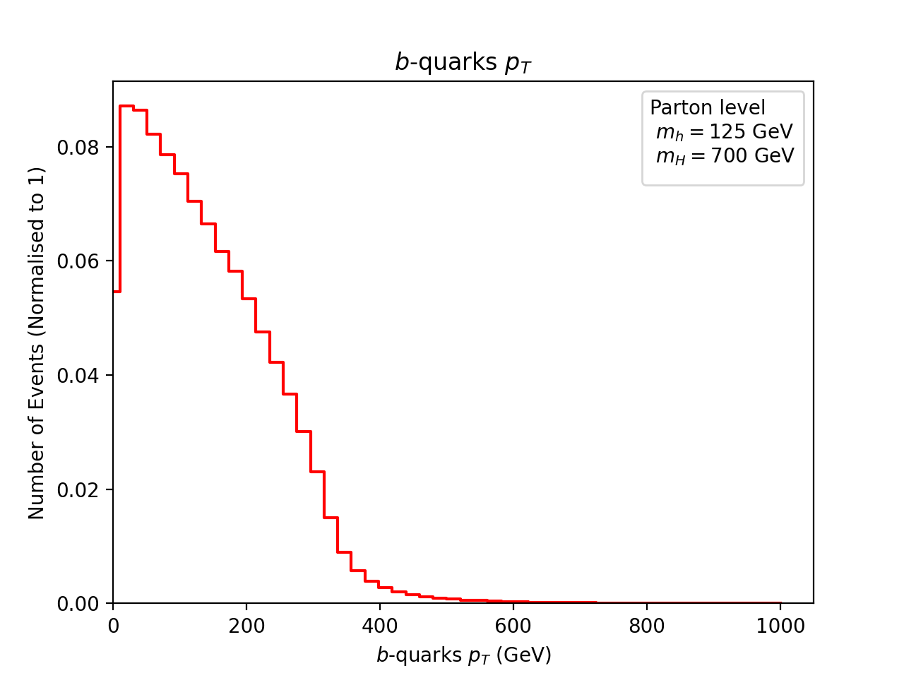
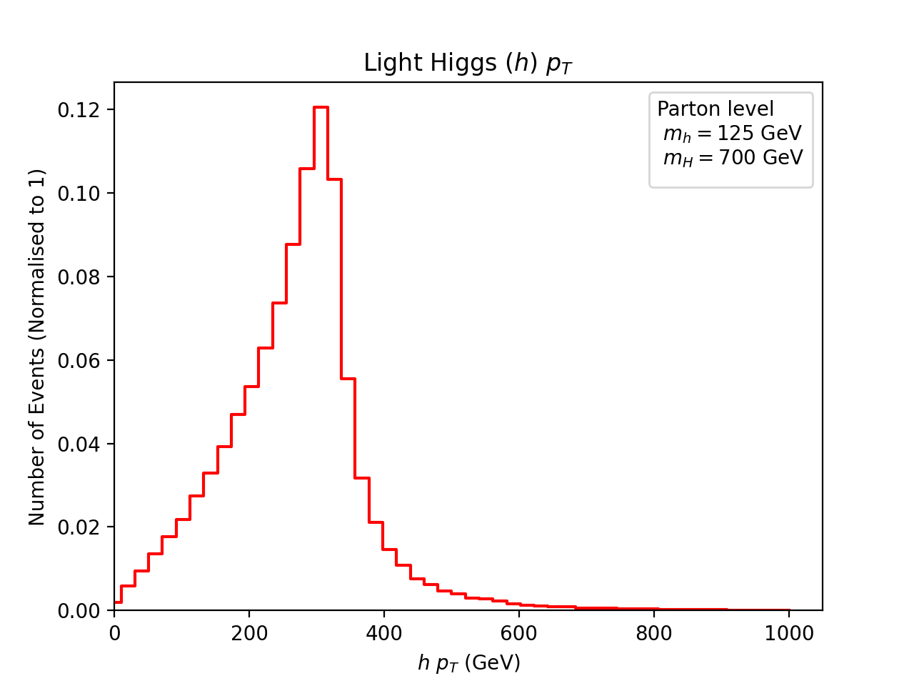
Figure 3: Transverse momenta of the final state $b$-quarks (left) and lights Higgses (right) before showering and hadronisation.

From Fig. 3 (left), we can see that the final state $b$-quarks have a wide range of momenta, well into $O(10^{2})$ GeV. The value of $\rho$, the variable-$R$ specific parameter, is generally chosen to be of the same order of magnitude as the jet $p_{T}$. However, looking at the $p_{T}$ distribution of the $b$-quarks, we perform a scan for $\rho$ over the region $[100,500]$ GeV to find an optimal value. Another point to mention here is that the light Higgs bosons are quite boosted, as seen from Fig. 3 (right). The angular separation in the $\eta-\phi$ plane between the pairs of Higgs bosons as well as $b$-quark pairs coming from the same Higgs boson crucially depend on the $p_{T}$ of the heavier and lighter Higgs bosons.

In Fig. 4, we see that the two light Higgs bosons are generally always back-to-back, their angular separation peaks being around $\pi$, which implies that the heavier Higgs boson is mostly produced at rest. Even though the heavier Higgs boson has very negligible $p_{T}$, due to the mass configuration of this BP, the two SM-like Higgses have a large momentum transfer from the heavy Higgs boson. The $b$-quarks originating from the lighter Higgs bosons, in contrast, tend to be closer together, i.e., collimated, which is an artefact of boosting.

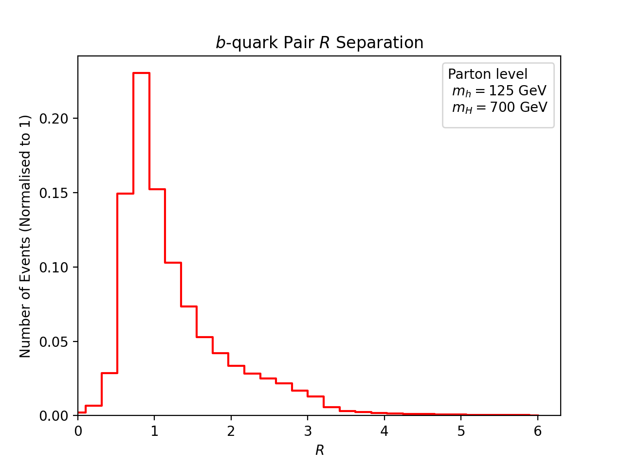
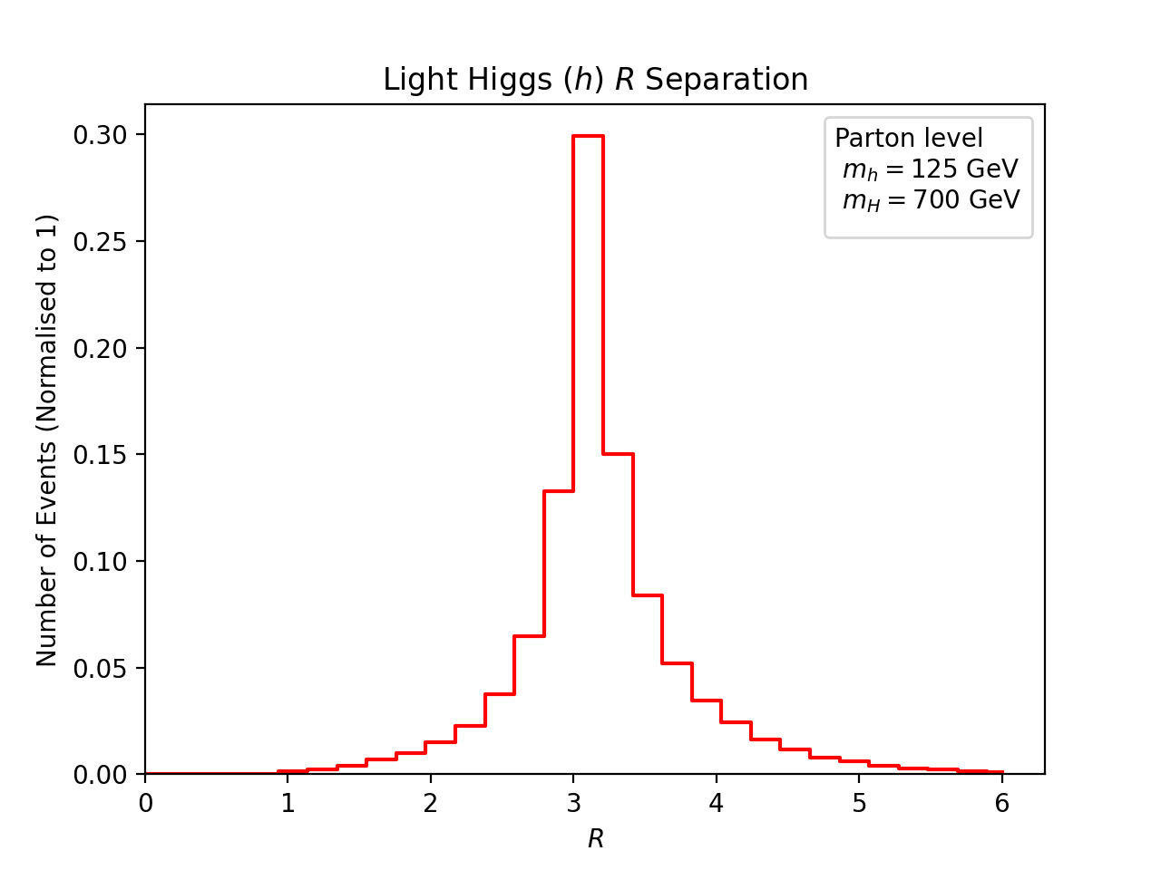
Figure 4: $\Delta R$ separation of the $b\bar{b}$ pair from a given Higgs (left) and between the two Higgses (right).

Consequently, the resulting jets from these $b$-partons will be close together in detector space. We can exploit this, and instead of trying to lower the values of $R$ in the jet clustering algorithm to ‘pick out’ and tag all four signal $b$-jets, we can instead use a deliberately large cone in order to capture two fat (and back-to-back) jets, wherein each contains both $b$-quarks coming from the decayed SM-like Higgs boson.

4.2 Jet Level Analysis

Now, informed by the parton level kinematics of the events, we can proceed to analyse this topology at the jet level. Using the anti-$k_{T}$ algorithm [10], we cluster EFlow objects obtained from after the fast detector simulation using Delphes into wide cone jets. We select those jets which have a $p_{T}>200$ GeV before we proceed to tag them, as described in Fig. 2.

Here, we compare two different methods of jet clustering for these double $b$-tagged fat jets. Firstly we use a large fixed cone size $R=1.0$ to construct two (nearly) back-to-back fat jets from each $h$ decay, which individually should reveal the mass of the SM-like Higgs boson . Secondly, we do the same but consider the variable-$R$ jet clustering algorithm [9]. We optimise the choice of $\rho$ to obtain the best reconstructed resonance mass peaks. For variable-$R$, we use $\rho=300$ with $R_{\rm min}=0.4$ and $R_{\rm max}=2.0$. These values are informed by the $p_{T}$ scale of the fixed cone $b$-jets and also the aforementioned scan on $\rho$.

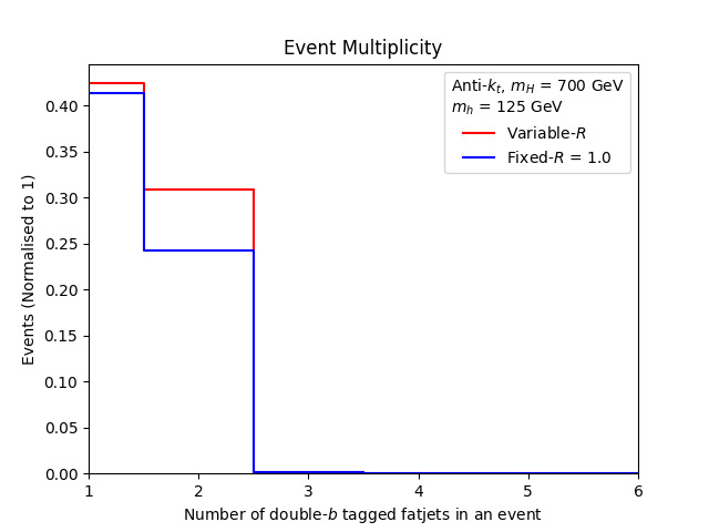
Figure 5: The double $b$-tagged fat jets multiplicity distribution for our BP.

In Fig. 5, we compare the $b$-jet multiplicity of the signal events for both fixed-$R$ and variable-$R$ algorithms. It is clear from the figure that we obtain more events with double-$b$ tagged fat jets for variable-$R$ than for fixed-$R=1.0$. The presence of more events containing double-$b$ tagged fat jets from the signal allows us to better reconstruct the Higgs resonance peaks in multi-jet mass distributions.

Next, to show the evidence of new physics, we reconstruct the mass of the resonances, namely the light and heavy Higgs bosons. We show the invariant masses of individual double $b$-tagged fat jets and the pair of double-$b$ tagged fat jets in Fig. 6. For $m_{h}$ mass resonance, we select the average of all double $b$-tagged jets.For $m_{H}$ resonance, we select events with two double $b$-tagged jets in order to recover heavy Higgs peak. It is evident that the peak of the variable-$R$ algorithm mass distributions is closer to the MC truth value of the corresponding Higgs boson masses, namely $m_{h}$ = 125 GeV and $m_{H}$ = 700 GeV.

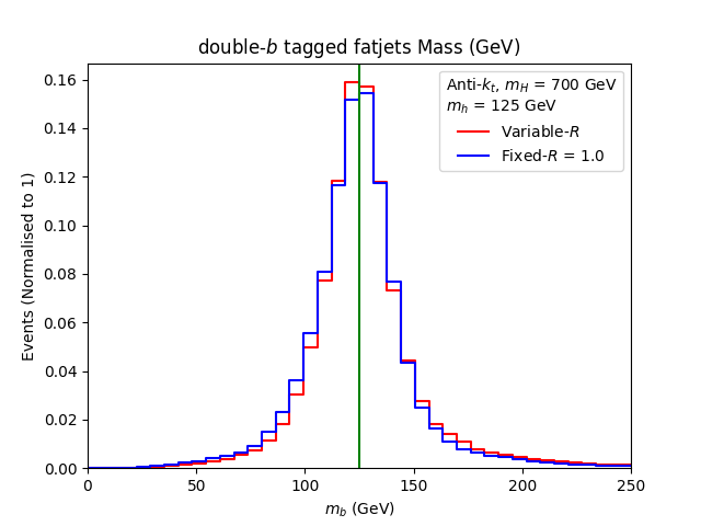
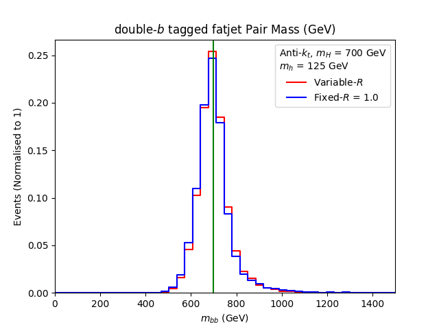
Figure 6: Right: The double $b$-tagged fat jets invariant mass $m_{h}$ for our BP. Left: The two double $b$-tagged fat jets invariant mass $m_{H}$ for our BP.

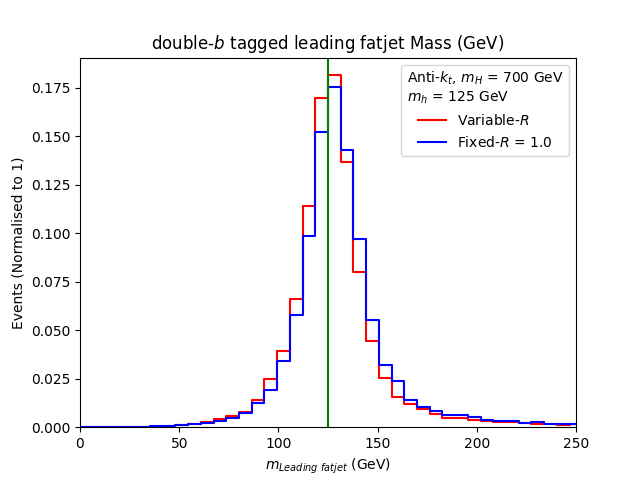
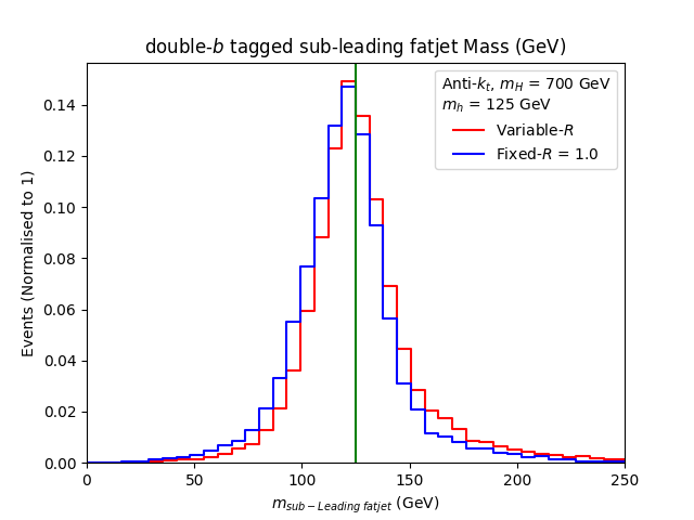
Figure 7: Right: The double $b$-tagged leading fat jet invariant mass $m_{h}$ for our BP. Left: The double $b$-tagged sub-leading fat jet invariant mass $m_{h}$ for our BP.

For completeness, we also present mass distributions for the leading and subleading fat jets (double $b$-tagged) in Fig. 7. The same behaviour can be seen here with variable-$R$ jet algorithm results being more aligned towards the corresponding MC truth value of the light Higgs boson mass. As a next step, we look at signal-to-background rates to compare the two jet reconstruction algorithms mentioned in the paper in this respect.

4.3 Signal-to-background Analysis

Here, we describe the performance of our final cuts used in extracting the signal from the backgrounds and compute the final significances in presence of both MPI and PU effects.

4.3.1 Signal-to-background Analysis with MPIs

In order to quantify the performance of the variable-$R$ algorithm against the fixed-$R$ one, we calculate signal-to-background rates and signal significances for the aforementioned two choices of integrated luminosity. To carry out this exercise, we apply the additional selection procedure

Figure 8: Additional event selection used to compute the final signal-to-background rates.

described in Fig. 8.

The event rates ($N$) for the various processes is given by:

$$N\ ={\rm Cross~{}section}~{}(\sigma)\times{\rm Luminosity}~{}(\mathcal{L}).$$ (11)

From Tabs. 2 and 3, it is evident that $pp\rightarrow b\bar{b}b\bar{b}$ is the dominant background process followed by $pp\rightarrow t\bar{t}$ and $pp\rightarrow Zb\bar{b}$. Upon using the two values of integrated luminosities ${\cal L}=$ $140$ fb^-1 and $300$ fb^-1, the next step is to calculate the significance rates ($\Sigma$) as a function of signal ($S$) and background ($B$) rates, which is given by:

$$\Sigma=\frac{N(S)}{\sqrt{N(B_{b\bar{b}b\bar{b}})+N(B_{t\bar{t}})+N(B_{Zb\bar{b}})}}.$$ (12)

Tab. 4 contains the significances for both choices of the jet clustering algorithm without and with QCD $K$-factors. The QCD $K$-factors describe the ratio between the leading and higher order cross sections. We have used $K$ = 2 (at NNLO level) for the signal [39, 40], $K$ = 1.5 (at NLO level) for $pp\rightarrow b\bar{b}b\bar{b}$ [41], $K$ = 1.4 (at NLO level) for $pp\rightarrow t\bar{t}$ [42] and $K$ = 1.4 (at NLO level) for $pp\rightarrow Zb\bar{b}$ [43]). It is clear that the variable-$R$ approach is more efficient compared to the fixed-$R$ method. The conclusion remains the same even after we take into account a typical 10% effect of systematic uncertainties in our calculation of signal significances.

We also present the significances for both choices of jet clustering algorithms without and with QCD $K$-factors using Trimming grooming techniques [44] to mitigate the effect of ISR and MPI in Tab. 5. We have used default CMS values for $R_{Trim}=0.2$ and $p_{T_{FracTrim}}=0.05$ taken from the Delphes CMS detector card. It is again clear that the variable-$R$ approach is more efficient compared to the fixed-$R$ method and our conclusions still hold even after the jets are groomed (one can always use other grooming techniques such as filtering [45], pruning [46], mass-drop [45], modified mass-drop [47] and soft drop [48], however, this is beyond the scope of this paper).

Process	Variable-$R$	$R=1.0$
	$m_{h}$ = 125 GeV, $m_{H}$ = 700 GeV	$m_{h}$ = 125 GeV, $m_{H}$ = 700 GeV
$pp\to H\to hh\rightarrow b\bar{b}b\bar{b}$	147.56	104.874
$pp\rightarrow t\bar{t}$	166.633	111.088
$pp\rightarrow b\bar{b}b\bar{b}$	592.336	435.139
$pp\rightarrow Zb\bar{b}$	0.067	0.063

Table 2: Event rates of signal and backgrounds for ${\cal L}=$ $140$ fb^-1 upon enforcing the initial cuts plus the mass selection criteria of Fig. 8 for the two jet reconstruction procedures.

Process	Variable-$R$	$R=1.0$
	$m_{h}$ = 125 GeV, $m_{H}$ = 700 GeV	$m_{h}$ = 125 GeV, $m_{H}$ = 700 GeV
$pp\to H\to hh\rightarrow b\bar{b}b\bar{b}$	316.2	224.73
$pp\rightarrow t\bar{t}$	357.071	238.047
$pp\rightarrow b\bar{b}b\bar{b}$	1269.292	932.441
$pp\rightarrow Zb\bar{b}$	0.145	0.135

Table 3: Event rates of signal and backgrounds for ${\cal L}=$ $300$ fb^-1 upon enforcing the initial cuts plus the mass selection criteria of Fig. 8 for the two jet reconstruction procedures.

	Variable-$R$	$R=1.0$
${\cal L}=$ $140$ fb-1	5.355	4.487
${\cal L}=$ $300$ fb-1	7.840	6.568

	Variable-$R$	$R=1.0$
${\cal L}=$ $140$ fb-1	8.810	7.377
${\cal L}=$ $300$ fb-1	12.897	10.799

Table 4: Left panel: Final $\Sigma$ values calculated upon enforcing the initial cuts plus the mass selection criteria of Fig. 8 for the two jet reconstruction procedures. Right panel: The same in presence of $K$-factors.

	Variable-$R$	$R=1.0$
${\cal L}=$ $140$ fb-1	5.753	4.861
${\cal L}=$ $300$ fb-1	8.421	7.116

	Variable-$R$	$R=1.0$
${\cal L}=$ $140$ fb-1	9.513	8.022
${\cal L}=$ $300$ fb-1	13.926	11.743

Table 5: Left panel: Final $\Sigma$ values calculated upon enforcing the initial cuts plus the mass selection criteria of Fig. 8 for the two jet reconstruction procedures using Trimming grooming techniques. Right panel: The same in presence of $K$-factors.

4.3.2 Signal-to-background Analysis with Pile-Up

As a final exercise, we want to check the performance of the two clustering algorithms used in this paper to reconstruct jets with Pile-Up (PU). As mentioned previously, to perform such a study one needs to apply proper detector simulation using Delphes. Specifically, generated events after hadronisation are passed through a Delphes CMS PU card. To generate the PU simulations, we have used Pythia8. Mixing of these PU events with the signal events is then done with $<N_{\rm PU}>$ = 50 for each hard scattering. Next, FastJet is implemented for both the variable-$R$ and anti-$k_{T}$ (with $R=1.0$) algorithms within the same card, to finally output jet information into a Root file. We finally carry out the analysis through a Root macro code using the same cutflow described in Section 3.2 in presence of the additional selection procedure described in Fig. 8.

We again calculate the signal-to-background rates, and consequent significances, in presence of the usual luminosities, specifically, for the purpose of comparing the performance of the variable-$R$ jet clustering algorithm against the anti-$k_{T}$ one with fixed $R=1.0$ in extracting the signal from the dominant backgrounds. The event rates ($N$) (described by Eq. (11)) for the various processes are given in Tabs. 6 and 7.

Process	Variable-$R$	$R=1.0$
	$m_{h}$ = 125 GeV, $m_{H}$ = 700 GeV	$m_{h}$ = 125 GeV, $m_{H}$ = 700 GeV
$pp\to H\to hh\rightarrow b\bar{b}b\bar{b}$	76.655	55.239
$pp\rightarrow t\bar{t}$	111.088	166.633
$pp\rightarrow b\bar{b}b\bar{b}$	423.748	282.498
$pp\rightarrow Zb\bar{b}$	0.0180	0.0270

Table 6: Event rates of signal and backgrounds for ${\cal L}=$ $140$ fb^-1 upon enforcing the initial cuts plus the mass selection criteria of Fig. 8 for the two jet reconstruction procedures.

Process	Variable-$R$	$R=1.0$
	$m_{h}$ = 125 GeV, $m_{H}$ = 700 GeV	$m_{h}$ = 125 GeV, $m_{H}$ = 700 GeV
$pp\to H\to hh\rightarrow b\bar{b}b\bar{b}$	164.260	118.371
$pp\rightarrow t\bar{t}$	238.047	357.071
$pp\rightarrow b\bar{b}b\bar{b}$	908.032	605.354
$pp\rightarrow Zb\bar{b}$	0.038	0.0580

Table 7: Event rates of signal and backgrounds for ${\cal L}=$ $300$ fb^-1 upon enforcing the initial cuts plus the mass selection criteria of Fig. 8 for the two jet reconstruction procedures.

	Variable-$R$	$R=1.0$
${\cal L}=$ $140$ fb-1	3.314	2.606
${\cal L}=$ $300$ fb-1	4.851	3.815

	Variable-$R$	$R=1.0$
${\cal L}=$ $140$ fb-1	5.450	4.309
${\cal L}=$ $300$ fb-1	7.978	6.309

Table 8: Left panel: Final $\Sigma$ values calculated calculated upon enforcing the initial cuts plus the mass selection criteria of Fig. 8 for the two jet reconstruction procedures. Right panel: The same in presence of $K$-factors.

Finally, Tab. 8 contains the final significance rates (as per Eq. (12)), again without and with $K$-factors. It is clear that the variable-$R$ approach is again more efficient compared to the fixed-$R$ method even with PU effects added.

5 Summary and Conclusions

In this paper, we have studied the performance of two different kinds of jet clustering algorithms at the LHC in accessing BSM signals induced by the cascade decays of a heavy Higgs boson $H$ (with a mass of 700 GeV) into a pair of SM-like Higgs states, $hh$. Given the mass difference between the two Higgs masses involved, the lighter Higgs bosons are produced with a large boost, so that their decays products, namely, a pair of $b$-quarks in our study, become highly collimated. We, therefore, reconstruct these events into two fat jets and perform a double $b$-tagging on these. For illustrative purposes, a 2HDM-II setup was assumed, by adopting a BP over its parameter space fully compliant with both theoretical and experimental constraints.

The two different kinds of jet clustering algorithms are a variable-$R$ one (where the cone size is not fixed but rather adapts to the resonant kinematics of the signal) and a more standard one, with a fixed cone size ($R=1$). These are used to reconstruct the mass of the lighter (SM-like) Higgs boson twice. Further, we select those events where a pair of such double $b$-tagged fat jets exist, in which total invariant mass reproduces the heavy Higgs boson mass. Through a cut-based signal-to-background analysis, we further find that the variable-$R$ method not only provides better reconstructed peaks of both Higgs boson masses, compared to the traditional algorithm, but also improves the signal-to-background ratio, which in turn results in higher signal significances at the LHC (altogether leading to potential discovery at both Run 2 and 3 of the LHC). Thus, we advocate the use of the former in establishing $pp\to H\to hh\to b\bar{b}b\bar{b}$ events in boosted topologies, in line with similar results previously obtained for the case of the same channel and different mass spectra yielding four slim $b$-jets. Finally, note that we have used the anti-$k_{T}$ algorithm as representative of the fixed cone size kind throughout but results are the same for the C/A jet clustering algorithm.

References

- [1] G. Aad et al. [ATLAS], Phys. Lett. B 716 (2012), 1-29 [arXiv:1207.7214 [hep-ex]].
- [2] S. Moretti and W. J. Stirling, Phys. Lett. B 347 (1995), 291-299 [Erratum: Phys. Lett. B 366 (1996), 451] [arXiv:hep-ph/9412209 [hep-ph]].
- [3] A. Djouadi, J. Kalinowski and P. M. Zerwas, Z. Phys. C 70 (1996), 435-448 [arXiv:hep-ph/9511342 [hep-ph]].
- [4] F. Gianotti, M. L. Mangano, T. Virdee et al. Eur. Phys. J. C 39 (2005), 293-333 [arXiv:hep-ph/0204087 [hep-ph]].
- [5] A. Chakraborty, S. Dasmahapatra, H. Day-Hall, B. Ford, S. Jain, S. Moretti, E. Olaiya and C. Shepherd-Themistocleous, [arXiv:2008.02499 [hep-ph]].
- [6] J. F. Gunion, H. E. Haber, G. L. Kane and S. Dawson, Front. Phys. 80 (2000), 1-404.
- [7] J. F. Gunion, H. E. Haber, G. L. Kane and S. Dawson, [arXiv:hep-ph/9302272 [hep-ph]].
- [8] G. C. Branco, P. M. Ferreira, L. Lavoura, M. N. Rebelo, M. Sher and J. P. Silva, Phys. Rept. 516 (2012), 1-102 [arXiv:1106.0034 [hep-ph]].
- [9] D. Krohn, J. Thaler and L. T. Wang, JHEP 06 (2009), 059 [arXiv:0903.0392 [hep-ph]].
- [10] M. Cacciari, G. P. Salam and G. Soyez, JHEP 04 (2008), 063 [arXiv:0802.1189 [hep-ph]].
- [11] G. P. Salam, Eur. Phys. J. C 67 (2010), 637-686 [arXiv:0906.1833 [hep-ph]].
- [12] J. Thaler and K. Van Tilburg, JHEP 03 (2011), 015 [arXiv:1011.2268 [hep-ph]].
- [13] A. Chakraborty, S. H. Lim, M. M. Nojiri and M. Takeuchi, JHEP 07 (2020), 111 [arXiv:2003.11787 [hep-ph]].
- [14] B. Bhattacherjee, C. Bose, A. Chakraborty and R. Sengupta, [arXiv:2212.11606 [hep-ph]].
- [15] A. J. Larkoski, I. Moult and B. Nachman, Phys. Rept. 841 (2020), 1-63 [arXiv:1709.04464 [hep-ph]].
- [16] G. Aad et al. [ATLAS], Phys. Lett. B 800 (2020), 135103 [arXiv:1906.02025 [hep-ex]].
- [17] M. Aaboud et al. [ATLAS], JHEP 01 (2019), 030 [arXiv:1804.06174 [hep-ex]].
- [18] A. M. Sirunyan et al. [CMS], Phys. Lett. B 781 (2018), 244-269 [arXiv:1710.04960 [hep-ex]].
- [19] V. Khachatryan et al. [CMS], Eur. Phys. J. C 76 (2016) no.7, 371 [arXiv:1602.08762 [hep-ex]].
- [20] V. N. Gribov and L. N. Lipatov, Sov. J. Nucl. Phys. 15, 675-684 (1972)
- [21] V. N. Gribov and L. N. Lipatov, Sov. J. Nucl. Phys. 15, 438-450 (1972) IPTI-381-71.
- [22] G. Altarelli and G. Parisi, Nucl. Phys. B 126, 298-318 (1977)
- [23] Y. L. Dokshitzer, Sov. Phys. JETP 46, 641-653 (1977)
- [24] G. F. Sterman and S. Weinberg, Phys. Rev. Lett. 39 (1977), 1436
- [25] S. Moretti, L. Lonnblad and T. Sjostrand, JHEP 08 (1998), 001 [arXiv:hep-ph/9804296 [hep-ph]].
- [26] M. Wobisch and T. Wengler, [arXiv:hep-ph/9907280 [hep-ph]].
- [27] Y. L. Dokshitzer, G. D. Leder, S. Moretti and B. R. Webber, JHEP 08 (1997), 001 [arXiv:hep-ph/9707323 [hep-ph]].
- [28] D. Eriksson, J. Rathsman and O. Stal, Comput. Phys. Commun. 181 (2010), 833-834
- [29] P. Bechtle, O. Brein, S. Heinemeyer, O. Stål, T. Stefaniak, G. Weiglein and K. E. Williams, Eur. Phys. J. C 74 (2014) no.3, 2693 [arXiv:1311.0055 [hep-ph]].
- [30] P. Bechtle, S. Heinemeyer, O. Stål, T. Stefaniak and G. Weiglein, Eur. Phys. J. C 74 (2014) no.2, 2711 [arXiv:1305.1933 [hep-ph]].
- [31] F. Mahmoudi, Comput. Phys. Commun. 180 (2009), 1718-1719.
- [32] R. D. Ball et al. [NNPDF], JHEP 04 (2015), 040 [arXiv:1410.8849 [hep-ph]].
- [33] J. Alwall, R. Frederix, S. Frixione, V. Hirschi, F. Maltoni, O. Mattelaer, H. S. Shao, T. Stelzer, P. Torrielli and M. Zaro, JHEP 07 (2014), 079 [arXiv:1405.0301 [hep-ph]].
- [34] T. Sjostrand, S. Mrenna and P. Z. Skands, Comput. Phys. Commun. 178 (2008), 852-867 [arXiv:0710.3820 [hep-ph]].
- [35] J. de Favereau et al. [DELPHES 3], JHEP 02 (2014), 057 [arXiv:1307.6346 [hep-ex]].
- [36] E. Conte, B. Fuks and G. Serret, Comput. Phys. Commun. 184 (2013), 222-256 [arXiv:1206.1599 [hep-ph]].
- [37] E. Conte and B. Fuks, Int. J. Mod. Phys. A 33 (2018) no.28, 1830027 [arXiv:1808.00480 [hep-ph]].
- [38] M. Cacciari, G. P. Salam and G. Soyez, Eur. Phys. J. C 72 (2012), 1896 [arXiv:1111.6097 [hep-ph]].
- [39] V. Ravindran, J. Smith and W. L. van Neerven, Nucl. Phys. B 665 (2003), 325-366 [arXiv:hep-ph/0302135 [hep-ph]].
- [40] R. V. Harlander and W. B. Kilgore, Phys. Rev. Lett. 88 (2002), 201801 [arXiv:hep-ph/0201206 [hep-ph]].
- [41] N. Greiner, A. Guffanti, T. Reiter and J. Reuter, Phys. Rev. Lett. 107 (2011), 102002 [arXiv:1105.3624 [hep-ph]].
- [42] T. Binoth et al. [SM and NLO Multileg Working Group], [arXiv:1003.1241 [hep-ph]].
- [43] F. Febres Cordero, L. Reina and D. Wackeroth, Phys. Rev. D 80 (2009), 034015 [arXiv:0906.1923 [hep-ph]].
- [44] D. Krohn, J. Thaler and L. T. Wang, JHEP 02 (2010), 084 [arXiv:0912.1342 [hep-ph]].
- [45] J. M. Butterworth, A. R. Davison, M. Rubin and G. P. Salam, Phys. Rev. Lett. 100 (2008), 242001 [arXiv:0802.2470 [hep-ph]].
- [46] S. D. Ellis, C. K. Vermilion and J. R. Walsh, Phys. Rev. D 80 (2009), 051501 [arXiv:0903.5081 [hep-ph]].
- [47] M. Dasgupta, A. Fregoso, S. Marzani and G. P. Salam, JHEP 09 (2013), 029 [arXiv:1307.0007 [hep-ph]].
- [48] A. J. Larkoski, S. Marzani, G. Soyez and J. Thaler, JHEP 05 (2014), 146 [arXiv:1402.2657 [hep-ph]].