A Framework for History-Aware Hyperparameter Optimisation in Reinforcement Learning

Abstract.

A Reinforcement Learning (RL) system depends on a set of initial conditions (hyperparameters) that affect the system’s performance. However, defining a good choice of hyperparameters is a challenging problem. Hyperparameter tuning often requires manual or automated searches to find optimal values. Nonetheless, a noticeable limitation is the high cost of algorithm evaluation for complex models, making the tuning process computationally expensive and time-consuming. In this paper, we propose a framework based on integrating complex event processing and temporal models, to alleviate these trade-offs. Through this combination, it is possible to gain insights about a running RL system efficiently and unobtrusively based on data stream monitoring and to create abstract representations that allow reasoning about the historical behaviour of the RL system. The obtained knowledge is exploited to provide feedback to the RL system for optimising its hyperparameters while making effective use of parallel resources. We introduce a novel history-aware epsilon-greedy logic for hyperparameter optimisation that instead of using static hyperparameters that are kept fixed for the whole training, adjusts the hyperparameters at runtime based on the analysis of the agent’s performance over time windows in a single agent’s lifetime. We tested the proposed approach in a 5G mobile communications case study that uses DQN, a variant of RL, for its decision-making. Our experiments demonstrated the effects of hyperparameter tuning using history on training stability and reward values. The encouraging results show that the proposed history-aware framework significantly improved performance compared to traditional hyperparameter tuning approaches.

1. Introduction

Reinforcement Learning (RL) is a sub-field of Machine Learning with a great success in applications such as self-driving cars, industry automation, among many others (Sutton and Barto, 2018). In RL, autonomous agents learn through trial-and-error how to find optimal solutions to a problem (Sutton and Barto, 2018). RL algorithms have multiple hyperparameters that require careful tuning as it is a core aspect of obtaining the state-of-the-art performance (Jomaa et al., 2019).

The search for the best hyperparameter configuration is a sequential decision process in which initial values are set, and later adjusted, through a mixture of intuition and trial-and-error, to optimise an observed performance to maximise the accuracy or minimise the loss (Jomaa et al., 2019). Hyperparameter Optimisation (HPO) often requires expensive manual or automated hyperparameter searches in order to perform properly on an application domain (Zahavy et al., 2020). However, a noticeable limitation is the high cost related to algorithm evaluation, which makes the tuning process highly inefficient, computational expensive, and commonly adds extra algorithm developing overheads to the RL agent decision-making processes (Zhang et al., 2021; Zahavy et al., 2020; Jomaa et al., 2019; Feurer and Hutter, 2019).

The full behaviour of complex RL systems often only emerges during operation. They thus need to be monitored at runtime to check that they adhere to their requirements (Rabiser et al., 2017). Event-driven Monitoring (EDM) is a common lightweight approach for monitoring a running system (Klar et al., 1992). Particularly, Complex Event Processing (CEP) is an EDM technique, for capturing, analysing, and correlating large amounts of data in real time in a domain-agnostic way (Luckham and Frasca, 1998). The present paper proposes the use of CEP to quickly detect causal dependencies between events on the fly by continuously querying data streams produced by the RL system in order to gain insights from events as they occur during the execution of the RL agent which is crucial for HPO (Feurer and Hutter, 2019).

CEP provides the short-term memory needed to analyse the system behaviour on pre-defined time-points or limited time-windows. However, it is debated that long-term memory is also required when analysing the effects of HPO on the RL agent to find optimal performance evolved on past behaviours. History-awareness requires node-level memory and traceability management facilities to allow the exploration of system’s history. Temporal Models (TMs) are seen to tackle these challenges (Gómez et al., 2018). TMs offer storage facilities that allows time representation using a temporal database (TDB) (Parra-Ullauri et al., 2021b, a). In this paper, a TDB supports the storage of massive amounts of historical data, while providing fast querying capabilities to support reasoning about runtime properties in the monitored RL agent.

In this paper, we propose a framework based on CEP ans TMs that can be reused for different RL algorithms. The proposed combination allows the detection of situations of interest at runtime and permits tracing the RL agent history to enable the short and long term memory required to analyse the impact of HPO. The framework uses a formal defined structure to trace data streams produced by the RL agents, process them and provide feedback for HPO. In addition, we present a novel history-aware epsilon-greedy logic for HPO that is implemented using the components of the proposed framework. This logic tunes the hyperparameter concurrently while acting greedily under certain circumstances, but also exploring the hyperparameter value-space with an $\epsilon$ probability in order to escape local maximums. The HPO occurs while the agent is learning, which turns to be more efficient than using static hyperparameters during the training process and having to update them on multiple agent’s lifetimes (Zahavy et al., 2020; Zhang et al., 2021).

In order to test the feasibility of the proposed framework, Deep Q-Network (DQN) (Sutton and Barto, 2018), a popular RL algorithm, was applied to a case study on the next generation of mobile communications from (Zheng et al., 2021). The experiments analysed the effects of the proposed history-aware approach for HPO during the RL agent training, and compared the results with traditional hyperparameter tuning approaches. Our experiments focused on updating the discounting factor hyperparameter at runtime for a single agent’s lifetime, using these different techniques.

The rest of the paper is organised as follows. Section 2 provides a description of the core concepts required to understand this paper. Section 3 introduces our approach. Experiments and results are presented in Section 4. The discussion is presented in Section 5. Section 6 compares the presented work with current state of HPO in RL. Finally, Section 7 presents conclusions and future directions.

2. Background

2.1. Hyperparameter Optimisation in Reinforcement Learning

In RL, an agent tries to maximise the optimal action-value function described as the Bellman Optimality Eq. (Sutton and Barto, 2018):

(1) $$Q^{*}(s,a)=\mathbb{E}\{r_{t+1}+\gamma*max_{a^{\prime}}Q^{*}(s_{t+1},a^{\prime})|s_{t}=s,a_{t}=a\}\vspace{-0.5 em}$$

where $\mathbb{E}$ represents the expected sum of future rewards characterised by the hyperparameter $\gamma$, which is the discounting factor (Sutton and Barto, 2018). A reward $r_{t}$ that occurs N steps in the future from the current state, is multiplied by $\gamma^{N}$ to describe its importance to the current state. As shown, defining the right $\gamma$ and additional hyperparameters through HPO is key to deliver optimal solutions in RL.

The most basic way of HPO is manual search, which is based on the intuition of the developer (Feurer and Hutter, 2019). Once the system execution has finished, the verification of convergence is reviewed. More sophisticated HPO approaches include i) Model-free Blackbox Optimisation (MBO) and ii) Bayesian Optimisation (BO) (Feurer and Hutter, 2019). Grid and random search are part of i). In grid search, the user defines a set of hyperparameter values to be analysed and the search evaluates the Cartesian product of these sets. Random search samples configurations at random until a certain budget for the search is exhausted. (Feurer and Hutter, 2019). Regarding ii), BO iteratively evaluates a promising hyperparameter configuration based on the current model then updates it trying to locate the optimum in multiple agent’s lifetimes. However, performing these techniques is time consuming, computationally expensive and requires expert knowledge (Fernandez and Caarls, 2018).

For the reasons mentioned, the introduction of an automated hyperparameter search process is key for the continuing success of RL and is acknowledged as the most basic task in automated machine learning (AutoML) (Feurer and Hutter, 2019). In this work we focus on MBO for a single agent’s lifetime, which is claimed to be more efficient than having static hyperparameters during the training process and updating them in multiple agent’s lifetimes (Zahavy et al., 2020; Zhang et al., 2021).

2.2. Temporal Models

TMs go beyond representing and processing the current state of systems (Gómez et al., 2018). They seek to add short and long-term memory to models through the use of temporal databases  (Mazak et al., 2020). Examples of temporal databases used for TMs, are Time Series Databases (TSDB) and Temporal Graph Databases (TGDB) (Mazak et al., 2020; Parra-Ullauri et al., 2021b). Each attribute to be monitored in a running system can be considered as a time series: a sequence of values along an axis (Esling and Agon, 2012). TGDB extend this ability to track the appearance and disappearance of entities and connections (Hartmann et al., 2017).

TGDBs record how nodes and edges appear, disappear and change their key/value pairs over time. Greycat (Hartmann et al., 2017) is an open-source TGDB. Nodes and edges in Greycat have a lifespan: they are created at a certain time-point, they may change in state over the various time-points, and they may be “ended” at another time-point. Greycat considers edges to be part of the state of their source and target nodes. It also uses a copy-on-write mechanism to store only the parts of a graph that changed at a certain time-point, thus saving disk space. In this work, TMs build on top of Greycat TGDB, allow accessing and retrieving causally connected historical information about runtime behaviour of RL agents.

2.3. Event-driven Monitoring

EDM approaches are commonly designed to monitor system events, processes and handle them in the background without interfering with the main system’s execution (Moser et al., 2010). Moser et al. identified in (Moser et al., 2010) four key requirements for EDM: i) it should be platform agnostic and unobtrusive, ii) it should be capable of integrating monitoring data from other subsystems, iii) it should enable monitoring across multiple services and instances, and iv) it should be capable of unveiling potential anomalies in the monitored system. CEP is a cutting-edge EDM technology that has been widely used to address these requirements (Luckham and Frasca, 1998).

CEP provides real-time analysis and correlation of large volumes of streaming data in an effective and efficient manner with the aim of automatically detecting situations of interest in a particular domain (event patterns). The patterns to be detected have to be defined and deployed into a CEP engine, i.e. the software responsible for analysing and correlating the data streams. Each CEP engine provides its own Event Processing Language (EPL) for implementing the patterns to be deployed. Among the existing CEP engines, we opted for Esper, a mature, scalable and high-performance CEP engine. The Esper EPL is a language similar to SQL but extended with temporal, causal and pattern operators, as well as data windows. The present document proposes to leverage the power of CEP to detect temporal and causal dependencies between events and to pre-process data streams, in order to gain insights from events as they occur during the training of an RL agent.

3. History-Aware Hyperparameter Optimisation for RL

This section presents our proposed framework integrating CEP and TMs for HPO. Additionally, the section also describes a novel history-aware epsilon-greedy logic that will be implemented using the referenced framework.

3.1. A Software Framework combining CEP and TMs for HPO

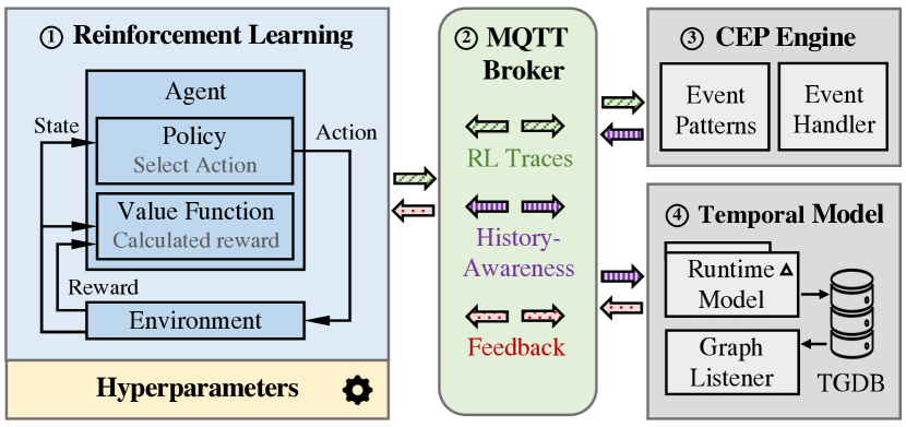
Figure 1. CEP and TMs for Hyperparameter Optimisation

RL involves challenging optimisation problems due to the stochasticity of evaluation, high computational cost and possible non-stationarity of the hyperparameters (Zhang et al., 2021). Therefore, the efficient continuous monitoring and dynamic verification of internal operations and parameters of the RL agent and its interactions with the environment over time are required. We propose the use of CEP for short-term analysis and TMs for navigation through the system history to provide feedback to the RL algorithm. Fig. 1 shows the proposed framework:

• The RL algorithm runs mostly independently from the rest of the system, while publishing data streams with logging information into an “RL Traces” topic created in a Message Queuing Telemetry Transport (MQTT) broker. The algorithm is subscribed to a “Feedback” topic, which will contain suggestions for hyperparameter change.

• The MQTT Broker is the communication hub for the architecture, acting as an event bus. It is responsible for loosely integrating the other components through the use of topics: components can publish events into a topic, or subscribe to updates about that topic.

• The CEP Engine is responsible for filtering and correlating data streams in the form of simple events coming from the RL algorithm into semantically richer complex events. It subscribes to the “RL Traces” topic to obtain those simple events, and it pushes complex events into the “History-Awareness” topic.

• The Temporal Model uses the complex events from the “History-Awareness” topic to construct the next version of the high-level model of the RL agent’s state, which is used to update the TM. A novel graph listener component is notified about the changes, which applies the HPO logic (see Section 3.2) to push any feedback on the current hyperparameter values into the “Feedback” MQTT topic.

TMs are conceptually structured according to a metamodel designed to record a Log of Decisions made by Agents, based on Observations about the environment, and including a set of Measurements of interest, according to various Measures. The metamodel is divided into two parts: the above concepts are defined into a core package from [omitted], and concepts that are specific to RL are split into its own package (see Fig. 2), which imports elements from the core package. The RL package provides a specialised RLAgent which keeps track of the RLState that can be observed in the environment, an RLDecision which tracks the QValues of each available action, and an RLObservation which tracks the current state before the action was taken, and the current Reward values.

Figure 2. Class diagram for the RL extensions to the core metamodel used to record system history. Imported core elements are marked with an arrow.

3.2. History-aware epsilon-greedy logic for HPO

In RL, the $N$-dimensional hyperparameter configuration space is defined as $\Lambda$ = $\Lambda_{1}\times...\times\Lambda_{N}$ and a vector of hyperparameters is denoted by $\lambda\in\Lambda$. Let’s denote the RL algorithm as $\Phi$ and $\Phi_{\lambda}$ the algorithm instantiated to a vector of hyperparameters $\lambda$. Let us define the objective function to maximise the value of a reward function $\mathcal{R}$. Then, we define the HPO problem of a $\Phi$ given the environment $E$ at time $T$ as finding the optimal hyperparameter vector $\lambda^{*}$:

(2) $$\lambda^{*}=\operatorname*{arg\,max}_{\lambda\in\Lambda}\mathcal{R}(\Phi_{\lambda},E,T)$$

where $\mathcal{R}(\Phi_{\lambda},E,T)$ measures a reward value generated by the algorithm $\Phi$ under a configuration of the $\lambda$ hyperparameter while interacting with the environment $E$ at time $T$.

Now we can introduce our history-aware epsilon-greedy approach. RL is episodic, with multiple iterations $i\in I$ performed within each episode $e\in E$ (Sutton and Barto, 2018). In this context, let us define the value of $\mathcal{R}$ at the instant $t_{i}$ after $\Phi_{\lambda}$ has interacted with the environment $E$ as the reward $r_{t}$ that the agent obtained by performing an action $a_{t}$ and arriving to the state $s_{t}$. Thus, the value of our reward function by iteration is denoted by $\mathcal{R}_{i}(t_{i},\lambda)=r_{t_{i}}$. Consequently, the reward function by episode is defined by:

(3) $$\mathcal{R}_{e}(t_{e},\lambda)=\frac{\sum_{i=1}^{I}\mathcal{R}_{i}(t_{i},\lambda)}{I}$$

After stated our reward function by episode, we define the criterion for analysing the history. In other words, how long back are we going to look when deciding to change a hyperparameter. With this purpose, we introduce the concept of time-windows to the logic. A time-window $w\in W$ consists of $x\in\mathbb{R}$ episodes $e$ where $x$ is the length of the time-window. Then, the value of our reward function by time-window is denoted by:

(4) $$\mathcal{R}_{win}(t_{w},\lambda)=\frac{\sum_{w=e}^{e+x-1}\mathcal{R}_{e}(t_{w},\lambda)}{x}$$

Eq. 4 defines the time frame when the monitoring process is taking place. The next step is to define the criterion that would lead to a hyperparameter update. The criteria selected is the stability of the reward value. We analyse the distance of the reward function by episode $\mathcal{R}_{e}$ to the mean of the time-window $\mathcal{R}_{win}$. If the value is below a defined threshold $th_{stable}\in\mathbb{R}$ for all the values within the time-window, we induce that the reward value has stabilised within a range and a possible hyperparameter update will be performed. Formalising this as a Boolean conjunction we have:

(5) $$\bigwedge_{j\in[e,e+x)}\left(|\mathcal{R}_{e}(t_{j},\lambda)-\mathcal{R}_{win}(t_{w},\lambda)|<th_{stable}\right)$$

where $\mathcal{R}_{win}$ is the reward function value for the time window at time $w=e+x-1$.

We have emphasised the word possible for a change in $\lambda$, as stability won’t necessarily mean that the agent has reached its maximum performance under the current conditions. Let’s consider the example when our optimiser system has observed the following set of $\mathcal{R}_{e}$ under the same conditions $\Phi_{\lambda}$, $\mathcal{R}:\{1,2,3,4,5,6\}$. We define a time-window length of 3 episodes ($x=3$) and a stability threshold of 2 ($th_{stable}=2$). Thus, $w_{1}=\{1,2,3\}$, $w_{2}=\{4,5,6\}$, $\mathcal{R}_{win_{1}}=2$ and $\mathcal{R}_{win_{2}}=5$. As a result, the Boolean conjunction for $w_{1}$ will be true. This would mean that the system requires a hyperparameter change. However, under the same conditions $\Phi_{\lambda}$, the system would have kept improving its performance as it is shown in $w_{2}$ and $\mathcal{R}_{win_{2}}$. Therefore, an additional condition is necessary to define when a hyperparameter tuning is required.

We introduce $max\mathcal{R}_{t}$ as the maximum known value of $\mathcal{R}_{win}$ up to the time-point $t$ and it is initialised as 0. Similarly, we introduce $max\lambda_{t}$ as the value of $\lambda$ that has produced $max\mathcal{R}_{t}$ up to the time-point $t$. We then define the main condition for hyperparameter tuning $HPO(\lambda)$ and it is described as follows:

(6) $$HPO(\lambda)=\begin{cases}\quad\begin{rcases}\lambda_{t},&\\ \quad\text{{with}}&\\ max\lambda_{t}\leftarrow\lambda_{t}&\\ max\mathcal{R}_{t}\leftarrow\mathcal{R}_{win_{t}}\quad\end{rcases}&\text{if }\mathcal{R}_{win_{t}}>max\mathcal{R}_{t}\\ \\ \quad\begin{rcases}\xi(\lambda),\qquad\qquad\qquad\quad\end{rcases}&\text{otherwise}\end{cases}$$

where $HPO(\lambda)$ is equal to $\lambda_{t}$ iff the current value of $\mathcal{R}_{win_{t}}$ is greater than the maximum known value of $max\mathcal{R}_{t}$ at time $t$. This would imply that the current value of our $\mathcal{R}$ function has increased from the previous maximum known and therefore the current configuration $\Phi_{\lambda_{t}}$ should be kept as the system is still ‘learning’. Correspondingly, the current value of $\mathcal{R}_{win_{t}}$ would become the new maximum known value of $max\mathcal{R}_{t}$ ($max\mathcal{R}_{t}\leftarrow\mathcal{R}_{win_{t}}$). In the case that the previous condition for $HPO(\lambda)$ is not met ($\mathcal{R}_{win_{t}}>max\mathcal{R}_{t}$), a hyperparameter tuning is required and will be analysed by our epsilon-greedy function $\xi(\lambda)$.

Our optimiser would examine $\xi(\lambda)$ iff and only iff the following conditions are met: i) $\mathcal{R}$ is stable for a time-window $w$ (Eq. 5), and ii) the current value of $\mathcal{R}_{win_{t}}$ is less than the previous maximum known value of $\mathcal{R}$, $max\mathcal{R}_{t}$. These conditions mean that the system is stable (regarding to rewards observed) and on a sub-optimal configuration of $\Phi_{\lambda_{t}}$ (on reference to $max\mathcal{R}_{t}$). Therefore, a different vector of hyperparameters $\lambda$ should be explored. The criterion for selecting the next $\lambda$ is a variation of the well-known epsilon ($\epsilon$)-greedy policy for balancing exploration and exploitation in RL (Sutton and Barto, 2018). The optimiser will explore the hyperparameter value-space with a probability of $\epsilon$, otherwise it will exploit the known best configuration ($max\lambda_{t}$). Thus, it would act greedily. Eq. 8 shows the proposed epsilon-greedy function $\xi(\lambda)$.

(7) $$\xi(\lambda)=\begin{cases}\quad\begin{rcases}max\lambda_{t},\qquad\quad\quad\end{rcases}&\text{with probability 1-$\epsilon$}\\ \\ \quad\begin{rcases}\text{random }\lambda\in\Lambda,&\\ \quad\text{{or}}&\\ \lambda+c,&\\ \quad\text{{or}}&\\ \lambda-c,\quad\end{rcases}&\text{with probability $\epsilon$}\end{cases}$$

In addition of exploring randomly the value-space with a probability $\epsilon$, we have introduced supplementary conditions that will help the optimiser for deciding if the current value of the hyperparameter to which it is performing the tuning should be increased to $\lambda+c$ or decreased to $\lambda-c$, where $c$ is a user-defined constant. These conditions give hints to the optimiser about the direction in the value-space where better performance is achieved.

Putting everything together, given a RL algorithm $\Phi$ that interacts with an environment $E$ at time $t\in T$ with an initial hyperparameter configuration $\lambda\in\Lambda$ such as $\Phi_{\lambda}$, its configuration will be analysed and possibly updated based on $HPO(\lambda)$ when meeting the stability condition on a time-window from (5). The update based on our $\epsilon$-greedy function $\xi(\lambda)$ will only take place if the observed value of our $\mathcal{R}$ for such a time-window is less than the best known value of $\mathcal{R}$, $max\mathcal{R}$. The advantage of the proposed approach is that exploration actions are only selected in situations when the system has stopped learning under the defined conditions, which is indicated by analysing the history of $\mathcal{R}$.

Finally, the found optimal hyperparameter vector $\lambda^{*}$ for a lifetime of the RL agent, corresponds to the final value of $max\lambda$:

(8) $$\lambda^{*}\leftarrow max\lambda$$

This history-aware epsilon-greedy logic for HPO in RL has been implemented using the architecture in Section 3.1, exploiting the benefits of CEP and TMs.

4. Experiments and Results

4.1. System under study: Airbone base stations

In order to demonstrate the feasibility of the proposed architecture, this section presents its implementation for a case study from the domain of mobile communications. In this case study, Airborne Base Stations (ABS) use DQN to decide where to move autonomously in order to provide connectivity to as many users as possible. The 5G Communications System Model performs the necessary calculations to estimate the Signal-to-Interference-plus-Noise Ratio (SINR) and the Reference Signal Received Power (RSRP) to defined if a user is connected or not (Zheng et al., 2021).

Developed by DeepMind in 2015, DQN has produced some breakthrough applications able to solve a wide range of Atari games even more efficiently than humans (Mnih et al., 2015). In contrast to tabular RL approaches, DQN avoids using a lookup table by instead predicting the Q-value of the current or potential states and actions using artificial neural networks (NN) or deep learning networks (Sutton and Barto, 2018). This Q-function (see Eq. 1) provides the expected discounted reward that results from taking an action $a_{t}$ in the state $s_{t}$ and policy $\pi$ is followed. The hyperparameters when training a DQN agent include the numbers of episodes and neurons, learning rate, exploration rate, discount factor, among others.

4.2. Experimentation: Scenario

For the current implementation, we decided to study the impact of optimising the discount factor as the key element in the Bellman equation after a non-exhaustive manual hyperparameter search. The discount factor determines how much the RL agents cares about rewards in the distant future relative to those in the immediate future (Sutton and Barto, 2018). The hyperparameter vector is expressed as follows:

$$\lambda(\gamma,\kappa)$$

where $\gamma$ represents the hyperparameter to be optimised (i.e. discount factor) and $\kappa$ the hyperparameters that remain fixed.

With these preliminaries, different experiments using the proposed framework were performed under the same scenario. It consisted of a training round (i.e. a single lifetime) of 100 episodes and 1000 steps for a set of 4 ABS with 1050 users scattered on a X-Y plane. The ABS try to maximise the number of users connected by performing actions (i.e. moving on different directions) and calculating the SINR to users on a collaborative fashion. Our main goal was trying to solve Eq. 2. With this purpose, two different experiments were defined:

• History-Aware HPO vs traditional HPO: In order to evaluate the proposed approach, we benchmarked it with traditional HPO techniques. Specifically, the previous mentioned (see Section 2), grid search and random search and BO. For the seek of the experiment, the hyperparameter tuning was performed uusing Optuna hyperpameter tool (Akiba et al., 2019) using these HPO techniques and during the training process. Thus during a single agent’s lifetime different of the common use of these approaches that requires the analysis on multiple agent’s lifetimes (Zahavy et al., 2020). In this context, the initial hyperparameters for each approach is described in table 1. From the literature (Sutton and Barto, 2018; Mnih et al., 2015), commonly used values for the discount factor are within the range of 0.9 and 0.99. We have included the manual setting with static discounting factor for comparison. For the case of grid search, in order to cover the hyperparameter-value space, the initial value of $\gamma$ is set to 0.9 and decays over the time with a rate of 0.1. Random search starts randomly, the history-aware HPO and BO start in the centre of the value-space.

• History-Aware HPO vs static hyperparameters: A second experiment was performed to analyse the impact of our approach in the performance of the system in comparison to keeping the hyperparameters static during the training. For this purpose, we initialised the training round with the same seeds and compared the reward evolution overtime for each hyperparameter configuration. The initial values of the discount factor that conformed the experiment were: $\gamma_{o}\in\{0.1,0.2,0.3,0.4,0.5,0.6,0.7,0.8,0.9\}$.

Approach	$\gamma_{o}$	Tuning criteria
Manual setting	0.9	static
Grid search	0.9	updated every 10 episodes
Random search	random	updated every 10 episodes
Bayesian Optimisation	0.5	updated every 10 episodes
History-aware HPO	0.5	automated-tuning

Table 1. Initial configuration for experiment 1

4.3. Experimentation: Setup

In order to test the feasibility of our approach, the history-aware epsilon-greedy logic for HPO presented in Section 3.2 was implemented using the different components of the proposed framework of Section 3.1. Accordingly, the process depicted in Fig. 1 is described next:

1. RL algorithm: DQN has been the selected RL approach for the system under study. The algorithm was extended to send the made decisions and observations in a trace log to a queue in a MQTT message broker in JSON format at each simulation step.

2. MQTT broker: The open-source Mosquitto was selected as communication hub. The different components are subscribed to topics that allow them to send and receive messages on the network using a publish/subscribe model.

3. CEP engine: It processes and correlates the trace logs received from the RL algorithm with the aim of detecting, in real time, the situations of interest for the application domain. A set of event patterns were implemented in the selected CEP engine (Esper). Precisely, we have implemented Equations 4, 5 and 6 using Esper EPL in a hierarchy of event patterns. Listing 1 shows the implementation of Equation 6 that attempts to detect stable conditions on time windows of 3 episodes ($w=3$) with a $th_{stable}=30$. Every pattern AvgByEpisode (which refers to Eq. 3), followed (->) by two subsequent AvgByEpisode and a EpiWinAVG (which refers to Eq. 4), is analysed (where statement) in compliance of the boolean conjunction of Eq. 5. When the condition is met (i.e. boolean conjunction = $True$), the engine automatically generates complex events that collect the required information, to therefore send the events to the MQTT broker component for further processing.

4. Temporal Model: It receives complex events and records their information as a new version of the model in the TGDB. Specifically, the Hawk model indexer was extended with the capability to subscribe to an MQTT queue and reshape the information into a model conforming to the metamodel in Fig. 2. The graph listener is notified when a stable condition is detected. Next, it performs the required calculations of Eq. 6 and 7 to provide feedback to the RL algorithm on either; keeping the hyperparameter configuration or tuning it towards finding a good solution to Eq. 2. The feedback provided is recorded as part of the temporal model enabling the long-term memory needed for further processing, accountability and post-mortem analysis.

Listing 1: Esper EPL pattern to select when the system is on an stable condition on a defined time-window

⬇

@public @buseventtype @Name(”isStableAVG”)

insert into isStableAVG

select w.averageWindow as avg,

w.episode as episode,

'CEP' as agent,

CAST(a3.drone_number as INT) as drone_number,

a3.step as step,

a3.gamma as gamma

from pattern [every a1 = AvgByEpisode ->

a2 = AvgByEpisode ->

a3 = AvgByEpisode ->

w = EpiWinAVG]

where

w.episode = a3.episode and

Math.abs(a1.avg-w.averageWindow) < 30 and

Math.abs(a2.avg-w.averageWindow) < 30 and

Math.abs(a3.avg-w.averageWindow) < 30

As previously mentioned, our implementation decouples the running RL-system from the HPO process. In that sense, the experiments were performed using two machines dedicated to different purposes: one performing the training of the different RL algorithms, and the other running the proposed framework. The RL algorithms ran on a dedicated ML server with 10 NVIDIA RTX A6000 48GB GPUs using the ABS simulator, Python 3, Anaconda 4.8.5, matplotlib 3.3.4, numpy 1.19.1, paho-mqtt 1.5.0, pandas 1.1.3, and pytorch 1.7.1. The machine running the proposed framework was a Lenovo Thinkpad T480 with an Intel i7-8550U CPU with 1.80GHz, running Ubuntu 18.04.2 LTS and Oracle Java 1.8.0_201, using Paho MQTT 1.2.2, Eclipse Hawk 2.0.0, and Esper 8.0.0. The full implementation can be found in (omitted for double-blind review).

4.4. Evaluation of the results

In this section, we present the evaluation of the results of using the proposed framework implementing the history-aware epsilon-greedy logic for HPO. We trained the DQN system under the same conditions for the different experiments. A total of 20 runs were conducted.

4.4.1. History-Aware HPO vs traditional HPO

The first experiment corresponded to a qualitative study of the performance of the ABS system using the proposed approach comparing against traditional HPO techniques. Fig. 3 shows the results. As it can be observed, our history-aware HPO approach (black line) over-performed, in terms of time to converge and accuracy, the different approaches obtaining its maximum values from episode 32 onward. The random search (blue line) fluctuates and its performance is closed with static configuration (red line). It is interesting to note that grid search (green line) achieved similar performance. However, the sharp dip at episode 70 to 80 shows a potential instability. Similarly, BO (green line) achieves maximum performance in episode 42 however, it could not recover after trails of sub-optimal hyperparameter values from episode 71 onwards.

The proposed approach allows us to get more insights about the HPO process by analysing the history stored in the TGDB in conformation of metamodel of 2. Fig. 4 (a) depicts the results. The extracted information shows that the maximum value of our reward value function $\mathcal{R}$ was 727.055 at episode 74 with $\gamma$=0.204. Therefore, under the configuration $\Phi_{\lambda(\gamma,\kappa)}$ the optimal found value for the HPO problem of Eq. 3 is: $\lambda^{*}\leftarrow\lambda(\gamma=0.204,\kappa)$.

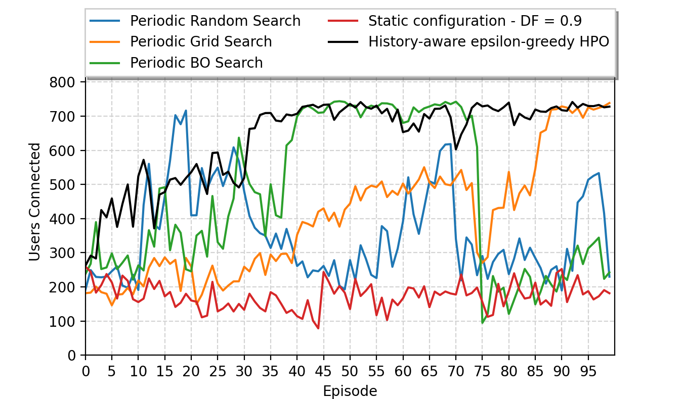
Figure 3. Comparison of hyperparameter tuning methods in DQN

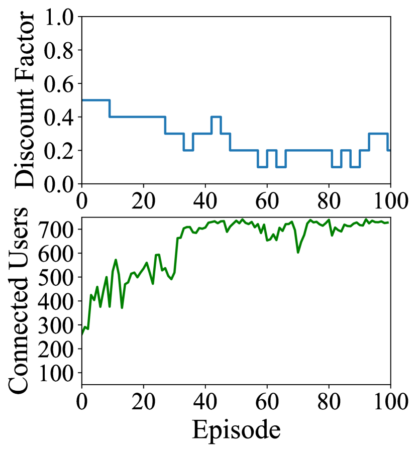
(a) Gamma = 0.5.

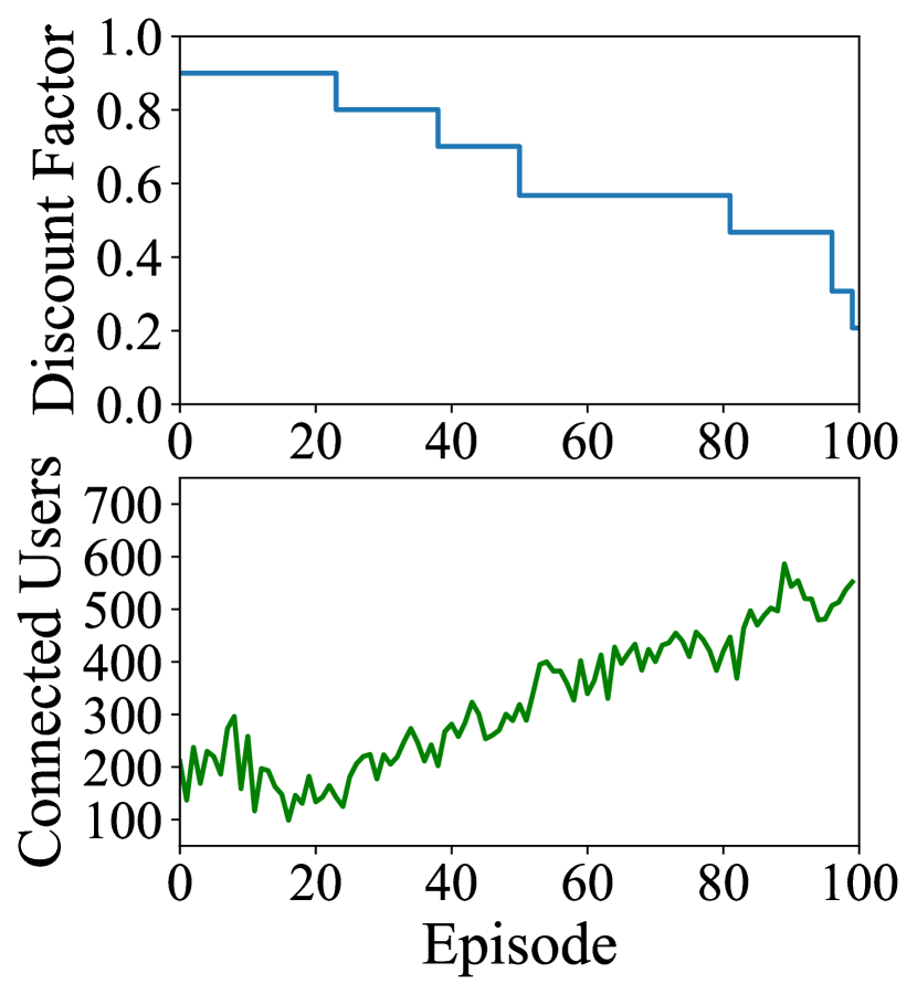
(b) Gamma = 0.9.

Figure 4. Reward and discount factor evolution, starting at $\gamma=0.5$ and $\gamma=0.9$ using history-aware HPO.

4.4.2. History-Aware HPO vs static hyperparameters

The second experiment included an exhaustive analysis of the performance of the RL algorithm using different seeds for the discount factor. The comparison include the analysis of the reward value function $\mathcal{R}$ with and without the proposed approach for each system configuration $\Phi_{\lambda_{t}(\gamma,\kappa)}$. The boxplots of Fig. 5 display the results. By using the proposed history-aware HPO (in red) the system was able to reach greater maximum values (the upper end of the whiskers) for each configuration. Furthermore, the iterquartile ranges (boxes) in each case had a greater upper quartile. Regarding to the medians, that represent the middle of the set, they were also greater for each case except for $\gamma=0.2$ and $\gamma=0.3$. This can suggest two things: i) the optimal values of $\gamma$ is within this range $0.2<\gamma^{*}<0.3$, which reinforce the result obtained in experiment 1, and ii) the variance in the data corresponds to the optimiser exploring the hyperparameter value-space with probability $\epsilon$. The results showed that by the use of the approach no outliers that lie on an abnormal distance from other values in the data set were found.

The best performance of the RL system using the history-aware HPO approach occurred when the initial value of the discounting factor was the centre of the hyperparameter value-space, $\gamma_{o}=0.5$ with an average of connected users of 636.104 and a median of 702.886. In the same manner, the poorest performance occurred with $\gamma_{o}=0.9$ with an average of 309.818 connected users and a median of 323.774. As shown in Fig. 4 (b), after exploring the hyperparameter value-space, the optimiser was going towards the optimal value of $\gamma$ which is corresponded with the increase of the reward. Thus, the system would have needed longer to find the optimal value.

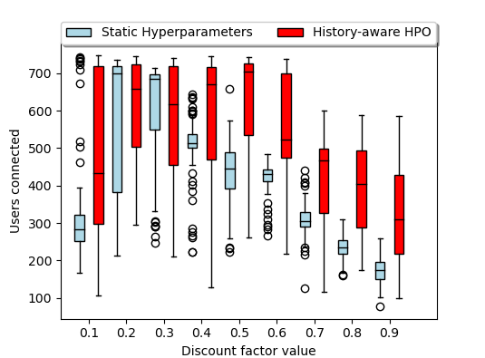
Figure 5. Comparison of history-aware hyperparameter optimisation vs static values

5. Discussion

The results from our conducted experiments showed the feasibility of the history-aware approach for HPO. Combining CEP and TMs made us to offer both the short and long term memory required for hyperparameter tuning with reflective capabilities. The history-aware epsilon-greedy logic allowed to explore the hyperparameter value-space with explicit long-term memory to remember good/optimal system’s configurations $\Phi_{\lambda_{t}(\gamma,\kappa)}$. Our experiments provide valuable insights into the effects of the tuning of the discount factor and its influence on the stability of training and overall system performance (maximised cumulative rewards).

The discount factor determines how many future time steps the agent considers when choosing an action. This value strongly depends on the environment that software agents are experienced. In the ABS case study, a discount factor close to 1 allows the agent to take actions very future oriented. A lower discount factor suggests that the ABS are more concerned to provide coverage to multiple users in short term but would introduce uncertainty in the long term. It is challenging to find the balance between the highest possible number of connected users in the short term and the long-term impact, as user behaviour may vary.

The approach has some limitations. Primarily, the optimisation of multiple hyperparameters in a single run. We have focused our study on the impact of the discount factor as key element of the Bellman Equation however, there are other hyperparameters that may affect the final system performance. Further work will involve the gradual lifting of these restrictions by allowing the tuning of multiple hyperparameters using different threads or timelines. Another limitation of the approach is the definition of stability on the system which is strongly related to the threshold of stability and time-window length. This could be problematic in situations when the $\mathcal{R}$ is noisy which could produce that the system never gets into a stable condition. This could be tackled by analysing different criteria for stability such as Z-score (Brase and Brase, 2013) and the absolute deviation around the median (Leys et al., 2013). Another approach could be introducing a patience time, e.g. if the system has not entered on a stable condition for X episodes, force it to explore another $\lambda$.

6. Related Work

HPO in the RL traditionally used a Delta-Bar-Delta method as incremental algorithms to tune parameters (Mahmood et al., 2012). However, this method and its variations were limited to linear supervised learning. The recent movement is to combine incremental Delta-Bar-Delta method and Temporal-difference learning  (Young et al., 2018). Those methods can not make tuning hyperparameters online and allow the algorithm to more robustly adjust to non-stationarity in a problem at the same time. A variety of techniques exist to combat this recently— most notably use of a large experience replay buffers or the use of multiple parallel actors. These techniques come at the cost of moving away from the online RL problem as it is traditionally formulated. More sophisticated approaches include Self-Tuning Actor Critic (STAC) (Zahavy et al., 2020) and Sequential Model-based Bayesian optimisation (SMBO) (Feurer and Hutter, 2019). However both methods ignored a crucial issue for RL: the possible non-stationarity of the RL problem induces a possible non-stationarity of the hyperparameters. Thereby, at various stages of the learning process, various hyperparameter settings might be required to behave optimally (Zhang et al., 2021). Furthermore, these approaches bases their functionality on multiple trials, thus multiple agent’s lifetimes different from the present work that focuses on HPO in a single lifetime.

Moreover, CEP can bring some advantages to ML approaches. They have been used together in fields such as the financial sector  (Luong et al., 2020), cybersecurity (Roldán et al., 2020) and Internet of Things (Ortiz et al., 2019). More particularly, CEP has been used to preprocess the stream of data that will be provided to the ML classifiers for training and predictive calculations (Luong et al., 2020). More evolved architectures include the use of ML to find and set event patterns for the detection of complex events, thus automatising the setup stage of a CEP system (Mehdiyev et al., 2015). Even more, some architectures have been developed to automatically update their event patterns using ML (Sun et al., 2020). ML and CEP are also combined to provide dynamic fault-tolerance support (Power and Kotonya, 2019).

Recently, CEP has been also integrated with TM to support both service monitoring and explainable reinforcement learning. Specifically, in (Parra-Ullauri et al., 2021b), an architecture based on CEP and TM is proposed for runtime monitoring of comprehensive data streams. This architecture promptly reacts to events and analyses the historic behaviour of a system. In (Parra-Ullauri et al., 2021b), a configurable architecture combining CEP and RL allows to keep track of a system’s reasoning over time, to extract on-demand history-aware explanations, to automatically detect situations of interest and to real-time filter the relevant points in time to be stored in a TGDB.

7. Concluding remarks and future work

Hyperparameter tuning is an omnipresent problem in RL as it is a key element for obtaining the state-of-the-art performance. This paper proposes to tackle this issue by integrating CEP and TMs. We investigated new ways to monitor software agents to explore their environment and pruning algorithms by automatically updating hyperparameters using feedback based on the RL agents historical behaviour. In order to test the feasibility of the approach, we conducted several experiments comparing the performance of a DQN case study using the proposed approach and different traditional HPO techniques.

The encouraging results show that the proposed framework combining CEP and TMs and implementing the history-aware epsilon-greedy logic significantly improved performance compared to traditional HPO approaches, in terms of reward values and learning speed. Furthermore, the outcomes from the monitoring process produce interpretable results easy for a human to understand and act upon. We have shown how some SE paradigms can be exploited for the benefit of RL and can be further used for creating accountability of RL systems. We believe that the SE and ML communities should work together to solve the critical challenges of assuring the quality of ML/RL and software systems in general.

Future work will include the study of the points mentioned in Section 5 regarding the the limitations of the approach. Further experiments will also be conducted to analyse the performance of the approach with other RL methods. Similarly, we will benchmark the proposed approach with more sophisticated HPO approaches as the ones mentioned in Section 6.

The feedback obtained from the proposed framework can be further exploited for example for safe early stopping (Khamaru et al., 2022). Moreover, by choosing a set of high-level operations from hyperparameter tuning to algorithm selection set, to guide an agent to perform various tasks, like remembering history, comparing and contrasting current and past inputs, and using learning methods to change its own learning methods, the proposed approach can be considered a first step towards Meta-Learning (Vanschoren, 2019). Finally, the obtained knowledge can be useful to convey this information for different stakeholders apart from proving feedback which can be another research direction.

References

- (1)
- Akiba et al. (2019) Takuya Akiba, Shotaro Sano, Toshihiko Yanase, Takeru Ohta, and Masanori Koyama. 2019. Optuna: A next-generation hyperparameter optimization framework. In Proceedings of the 25th ACM SIGKDD international conference on knowledge discovery & data mining. 2623–2631.
- Brase and Brase (2013) Charles Henry Brase and Corrinne Pellillo Brase. 2013. Understanding basic statistics. Brooks/Cole Cengage Learning.
- Esling and Agon (2012) Philippe Esling and Carlos Agon. 2012. Time-series data mining. ACM CSUR 45, 1 (2012).
- Fernandez and Caarls (2018) Franklin Cardeñoso Fernandez and Wouter Caarls. 2018. Parameters tuning and optimization for reinforcement learning algorithms using evolutionary computing. In 2018 International Conference on Information Systems and Computer Science.
- Feurer and Hutter (2019) Matthias Feurer and Frank Hutter. 2019. Hyperparameter optimization. In Automated machine learning.
- Gómez et al. (2018) Abel Gómez, Jordi Cabot, and Manuel Wimmer. 2018. TemporalEMF: A temporal metamodeling framework. In International Conference on Conceptual Modeling.
- Hartmann et al. (2017) Thomas Hartmann, Francois Fouquet, et al. 2017. Analyzing Complex Data in Motion at Scale with Temporal Graphs. In Proceedings of SEKE’17.
- Jomaa et al. (2019) Hadi S Jomaa, Josif Grabocka, and Lars Schmidt-Thieme. 2019. Hyp-rl: Hyperparameter optimization by reinforcement learning. arXiv preprint arXiv:1906.11527 (2019).
- Khamaru et al. (2022) Koulik Khamaru, Eric Xia, Martin J Wainwright, and Michael I Jordan. 2022. Instance-Dependent Confidence and Early Stopping for Reinforcement Learning. arXiv preprint arXiv:2201.08536 (2022).
- Klar et al. (1992) Rainer Klar, Andreas Quick, and Franz Soetz. 1992. Tools for a Model-driven Instrumentation for Monitoring. In Proceedings of the 5th International Conference on Modelling Techniques and Tools for Computer Performance Evaluation.
- Leys et al. (2013) Christophe Leys, Christophe Ley, Olivier Klein, Philippe Bernard, and Laurent Licata. 2013. Detecting outliers: Do not use standard deviation around the mean, use absolute deviation around the median. Journal of experimental social psychology (2013).
- Luckham and Frasca (1998) David C Luckham and Brian Frasca. 1998. Complex event processing in distributed systems. Computer Systems Laboratory Technical Report CSL-TR-98-754. Stanford University, Stanford (1998).
- Luong et al. (2020) Nhan Nathan Tri Luong, Zoran Milosevic, Andrew Berry, and Fethi Rabhi. 2020. An open architecture for complex event processing with machine learning. In 2020 IEEE 24th International Enterprise Distributed Object Computing Conference.
- Mahmood et al. (2012) Ashique Rupam Mahmood, Richard S Sutton, Thomas Degris, and Patrick M Pilarski. 2012. Tuning-free step-size adaptation. In 2012 IEEE International Conference on Acoustics, Speech and Signal Processing.
- Mazak et al. (2020) Alexandra Mazak, Sabine Wolny, Abel Gómez, Jordi Cabot, Manuel Wimmer, and Gerti Kappel. 2020. Temporal models on time series databases. J. Object Technol (2020).
- Mehdiyev et al. (2015) Nijat Mehdiyev, Julian Krumeich, David Enke, Dirk Werth, and Peter Loos. 2015. Determination of Rule Patterns in Complex Event Processing Using Machine Learning Techniques. Procedia Computer Science 61 (2015).
- Mnih et al. (2015) Volodymyr Mnih, Koray Kavukcuoglu, David Silver, Andrei A Rusu, Joel Veness, Marc G Bellemare, Alex Graves, Martin Riedmiller, Andreas K Fidjeland, Georg Ostrovski, et al. 2015. Human-level control through deep reinforcement learning. nature 7540 (2015).
- Moser et al. (2010) Oliver Moser, Florian Rosenberg, and Schahram Dustdar. 2010. Event driven monitoring for service composition infrastructures. In International Conference on Web Information Systems Engineering.
- Ortiz et al. (2019) Guadalupe Ortiz, Jose Antonio Caravaca, Alfonso Garcia-de Prado, Francisco Chavez de la O, and Juan Boubeta-Puig. 2019. Real-Time Context-Aware Microservice Architecture for Predictive Analytics and Smart Decision-Making. IEEE Access (2019).
- Parra-Ullauri et al. (2021a) Juan Marcelo Parra-Ullauri, Antonio García-Domínguez, Juan Boubeta-Puig, Nelly Bencomo, and Guadalupe Ortiz. 2021a. Towards an architecture integrating complex event processing and temporal graphs for service monitoring. In Proceedings of the 36th Annual ACM Symposium on Applied Computing. 427–435.
- Parra-Ullauri et al. (2021b) Juan Marcelo Parra-Ullauri, Antonio García-Domínguez, Nelly Bencomo, Changgang Zheng, Chen Zhen, Juan Boubeta-Puig, Guadalupe Ortiz, and Shufan Yang. 2021b. Event-driven temporal models for explanations - ETeMoX: explaining reinforcement learning. Software and Systems Modeling (2021).
- Power and Kotonya (2019) Alexander Power and Gerald Kotonya. 2019. Providing Fault Tolerance via Complex Event Processing and Machine Learning for IoT Systems. In Proceedings of the 9th International Conference on the Internet of Things (IoT 2019). Association for Computing Machinery, New York, NY, USA.
- Rabiser et al. (2017) Rick Rabiser, Sam Guinea, Michael Vierhauser, Luciano Baresi, and Paul Grünbacher. 2017. A comparison framework for runtime monitoring approaches. Journal of Systems and Software (2017).
- Roldán et al. (2020) José Roldán, Juan Boubeta-Puig, José Luis Martínez, and Guadalupe Ortiz. 2020. Integrating Complex Event Processing and Machine Learning: an Intelligent Architecture for Detecting IoT Security Attacks. Expert Systems with Applications 149 (2020).
- Sun et al. (2020) Yunhao Sun, Guanyu Li, and Bo Ning. 2020. Automatic Rule Updating based on Machine Learning in Complex Event Processing. In 2020 IEEE 40th International Conference on Distributed Computing Systems.
- Sutton and Barto (2018) Richard S Sutton and Andrew G Barto. 2018. Reinforcement learning: An introduction. MIT press.
- Vanschoren (2019) Joaquin Vanschoren. 2019. Meta-learning. In Automated Machine Learning.
- Young et al. (2018) Kenny Young, Baoxiang Wang, and Matthew E Taylor. 2018. Metatrace: Online step-size tuning by meta-gradient descent for reinforcement learning control. arXiv preprint arXiv:1805.04514 (2018).
- Zahavy et al. (2020) Tom Zahavy, Zhongwen Xu, Vivek Veeriah, Matteo Hessel, Junhyuk Oh, Hado van Hasselt, David Silver, and Satinder Singh. 2020. Self-tuning deep reinforcement learning. arXiv preprint arXiv:2002.12928 (2020).
- Zhang et al. (2021) Baohe Zhang, Raghu Rajan, Luis Pineda, Nathan Lambert, André Biedenkapp, Kurtland Chua, Frank Hutter, and Roberto Calandra. 2021. On the importance of hyperparameter optimization for model-based reinforcement learning. In International Conference on Artificial Intelligence and Statistics.
- Zheng et al. (2021) Changgang Zheng, Shufan Yang, Juan Marcelo Parra-Ullauri, Antonio Garcia-Dominguez, and Nelly Bencomo. 2021. Reward-reinforced generative adversarial networks for multi-agent systems. IEEE Transactions on Emerging Topics in Computational Intelligence (2021).