Blind2Sound: Self-Supervised Image Denoising without Residual Noise

Abstract

Self-supervised blind denoising for Poisson-Gaussian noise remains a challenging task. Pseudo-supervised pairs constructed from single noisy images re-corrupt the signal and degrade the performance. The visible blindspots solve the information loss in masked inputs. However, without explicitly noise sensing, mean square error as an objective function cannot adjust denoising intensities for dynamic noise levels, leading to noticeable residual noise. In this paper, we propose Blind2Sound, a simple yet effective approach to overcome residual noise in denoised images. The proposed adaptive re-visible loss senses noise levels and performs personalized denoising without noise residues while retaining the signal lossless. The theoretical analysis of intermediate medium gradients guarantees stable training, while the Cramer Gaussian loss acts as a regularization to facilitate the accurate perception of noise levels and improve the performance of the denoiser. Experiments on synthetic and real-world datasets show the superior performance of our method, especially for single-channel images. The code is available in supplementary materials.

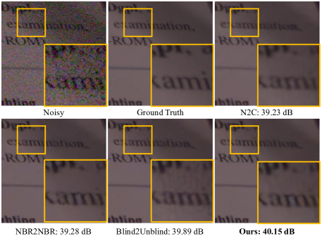
Figure 1: Real-world image denoising on the SIDD validation. Our approach performs thorough noise removal, while Blind2Unblind has considerable noise artifacts.

1 Introduction

Supervised image denoisers [34, 43, 44, 17, 4, 39, 41] have demonstrated impressive and superior performance by utilizing numerous noisy-clean pairs. Notably, several researchers [34, 43, 44] pioneered the removal of additive white Gaussian noise and achieved notable performance gains. These denoisers [17, 4, 39, 41] can also eliminate other noise patterns, especially signal-dependent noise in the real world. However, acquiring a large amount of paired data to train a denoiser can be costly and, in some cases, such as CT and MRI, even impossible. Moreover, the performance of these denoisers rapidly degrades once they encounter unknown noise patterns due to the inherent prior embedded in the training data.

To tackle the challenge of acquiring paired data, researchers have conducted numerous studies [7, 40, 12, 37, 25, 22, 5] in two categories: data synthesis and self-supervised denoisers. Data synthesis involves generating paired data for supervised training via adding noise to clean images. For instance, UPI [7] and CycleISP [40] analyze the operations of the camera imaging pipeline on signal-dependent noise and create an imaging framework capable of generating arbitrary real image pairs in both raw-RGB and sRGB space. Other researchers [12, 37] synthesize noisy-clean image pairs for training using pre-estimated noise parameters. However, while data synthesis approaches are effective with limited specific data, their poor generality limits their broader application.

Noise2Noise [25], a special case of supervised denoising that uses corrupted image pairs, serves as the foundation for self-supervised denoising. Self-supervised denoisers, which learn only from a single raw noise image, have become the leading solution for denoising without data collection limitations. Blindspot schemes, including manual masking [22, 5] and blindspot networks (BSN) [23, 37, 10, 9], enable single image denoising by assuming that the signal is context-dependent and the noise is irrelevant. However, the information loss and sub-optimal masking strategies degrade the upper bound of denoising performance. Some works [38, 30, 31] introduce additional noise to construct training data pairs. The pre-calibrated noise level restricts their application, and the re-corruption worsens the loss of valuable signals. NBR2NBR [20] sub-samples low-resolution training pairs from single noisy images for supervised training. The surrounding pixel approximation results in over-smoothing and block artifacts. FBI-Denoiser (FBI-D) [8] reimplements Gaussian estimation [11] as tensor operations combined with Generalized Anscombe Transformations (GAT) [3] to formulate Gaussian loss. However, Gaussian loss without fine-grained constraints zooms noise estimation errors. AP-BSN [24] breaks spatial correlation but remains in the scope of BSN. Blind2Unblind [36] achieves lossless denoising using the re-visible transition, but the greedy pixel-level fitting without noise sensing leads to sizable residual noise.

In this paper, we present a novel framework named Blind2Sound for self-supervised blind denoising, which achieves personalized denoising without noise residues while ensuring signal lossless. The framework includes an adaptive re-visible loss for lossless and personalized denoising and a Cramer Gaussian loss as a regularization to accurately sense noise knowledge. The framework assumes that the masked and visible branches are two independent generative processes, while denoising results following normal distributions and the respective noise following a Poisson-Gaussian distribution. This independence ensures that the masked results do not suppress the visible denoising. For optimal denoising, the adaptive loss adjusts noise removal via noise levels, while compatible with the lossless re-visible framework. The adaptive loss consists of two branches and their noise parameters, and the masked branch as an intermediate medium for gradient update. Due to signal dependence, the bottleneck of the masked branch greatly suppresses the accuracy of Poisson noise. Thus, the weighted Poisson noises in the mixed marginal likelihood is simplified to a single Poisson component. Moreover, the Cramer Gaussian loss introduces fine-grained noise knowledge, including sub-block and cross-channel constraints, to boost the estimation accuracy.

Our contribution can be summarized in three aspects:

1. The proposed self-supervised denoising framework adjusts denoising intensities based on sensed noise levels, achieving personalized denoising without residual noise while the signal is lossless.

2. We provide theoretical analysis for adaptive re-visible loss and the gradient of intermediate medium.

3. Our approach shows excellent performance on various real-world datasets with dynamic noise patterns.

2 Related Work

Self-Supervised Blind Image Denoising  Although Noise2Noise [25] makes collecting paired data much easier, it remains impractical as it requires noisy image pairs from the same source. Therefore, blindspot schemes such as manual masking [22, 5] and blindspot networks [23, 10] have been developed to achieve self-supervised denoising. However, these schemes suffer from the loss of valuable information, leading to severe artifacts. To address this issue, several methods, such as Laine19 [23], DBSN [37], FC-AIDE [10], BP-AIDE [9], and AP-BSN [24], have been proposed to enhance BSN. However, these methods either have poor performance or slow inference on Poisson-Gaussian noise. FBI-D [8] proposes a fast and effective blind image denoiser for Poisson-Gaussian noise, but its noise estimator has low accuracy in sRGB space without fine-grained noise constrains. Besides, the post-processing step can reinforce denoising errors accumulated in previous steps. Blind2Unblind [36] overcomes these limitations and achieves fast lossless denoising under blindspots. However, implicit denoising without sensing noise levels is unable to provide personalized noise removal for Poisson-Gaussian noise, resulting in residual noise artifacts.

Noise Estimation Methods  Current noise estimation methods [26, 33, 11, 15, 27] are mainly designed for two noise models: additive white Gaussian noise (AWGN) and Poisson-Gaussian noise. For AWGN, a signal-independent noise, once the noise variance is known, its distribution can be determined. Previous methods [26, 33] for estimating AWGN variance used low-rank patch selection and principal component analysis. Recently, Chen et al. [11] addressed the bias issue for Gaussian parameter estimation using statistical decomposition of eigenvalues. In contrast, Poisson-Gaussian noise [15] is a mixture of Poisson and Gaussian components and is often considered as source-related noise in real-world scenarios. Foi et al. [15] introduced the Poisson-Gaussian model and provided fully automated noise parameter estimation for a single noisy image. More recently, Liu et al. [27] improved local mean and noise variance estimation for selected low-rank patches.

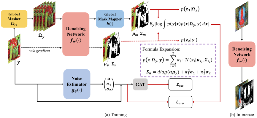
Figure 2: The architecture of the proposed Blind2Sound framework. The masked volume is represented by $\boldsymbol{\Omega_{y}}$, and the dotted lines indicate the forward process without updating the gradient. The Global Masker and Global Mask Mapper are detailed in the Supplementary Material (S.M.). Note that the noise estimator and the denoiser are trained through joint optimization. During inference, the auxiliary branches, namely the noise estimator and masked branch, are removed, and the denoiser directly generates denoised images from raw noisy inputs $\boldsymbol{y}$.

3 Problem Setting and Preliminaries

3.1 Problem Formulation

Given a noisy observation $\boldsymbol{y}$, our goal is to learn the clean image $\boldsymbol{x}$ and its noise parameters directly from a single noisy image. We focus on Poisson-Gaussian noise [15], which is common in real-world imaging sensors. The noise-corrupted observation $\boldsymbol{y}$ can be described as follows:

$$\boldsymbol{y}=\alpha P+N,$$ (1)

where $P\sim\rm{Poisson}(\boldsymbol{x}/\alpha)$ is the signal-dependent Poisson noise caused by photon counting, and $N\sim\mathcal{N}(0,\sigma^{2})$ is the signal-independent Gaussian noise resulting from electric and thermal noise. Here, $\alpha$ is a scaling factor that depends on the quantum efficiency and analog gain. To simplify the problem, the Poisson noise is approximated as signal-independent Gaussian noise [18], and the corruption can be reformulated as:

$$\boldsymbol{y}=\boldsymbol{x}+\mathcal{N}(0,\alpha\boldsymbol{x}+\sigma^{2}).$$ (2)

3.2 Generalized Anscombe Transformation (GAT)

GAT [3] is a popular variance-stabilized transform used for Poisson-Gaussian noise. It converts the mixture noise into stable Gaussian noise with unit variance:

$$G_{\alpha,\sigma}(\boldsymbol{y})=\frac{2}{\alpha}\sqrt{\alpha\boldsymbol{y}+\frac{3}{8}\alpha^{2}+\sigma^{2}}.$$ (3)

3.3 Gaussian Loss

As discussed in Section 1, Byun et al. [8] introduce a noise estimation network, denoted as $h_{\boldsymbol{\theta}}(\cdot)$, that takes Poisson-Gaussian noise-corrupted images $\boldsymbol{y}$ as input and produces the estimated noise parameters $(\hat{\alpha},\hat{\sigma})$. To train this network, they reimplement the Gaussian parameter estimation proposed in [11] as tensor operations $\eta(\cdot)$ and leverage the property that the transformed noise level using GAT should be closed to unit variance. Therefore, the Gaussian loss is defined for noise estimation as:

$$\mathop{\arg\min}\limits_{\boldsymbol{\theta}}\mathbb{E}_{\mathbf{y}}\left\|\eta\left(G_{\hat{\alpha}\left(\boldsymbol{\theta}\right),\hat{\sigma}\left(\boldsymbol{\theta}\right)}\left(\boldsymbol{y}\right)\right)-1\right\|^{2}_{2},$$ (4)

the noise estimation network $h_{\boldsymbol{\theta}}(\boldsymbol{y})$ predicts the noise parameters $\hat{\alpha}\left(\boldsymbol{\theta}\right)$ and $\hat{\sigma}\left(\boldsymbol{\theta}\right)$. Then, the transformed noisy image with unit variance is denoised and the output of BSN is mapped back to the original image using the Inverse Anscombe transformation (IAT) [28]. Note that noise estimation and denoising are trained separately without joint optimization.

3.4 Blind2Unblind Revisit

Blind2Unblind [36] is a self-supervised noise removal method that achieves lossless denoising using the re-visible transition. The overall framework consists of two branches: a masked branch that uses pseudo-supervised pairs for auxiliary denoising and a visible branch that learns directly from raw noise images. Given the noisy observation $\mathbf{y}$, Blind2Unblind minimizes the following re-visible loss:

$$\mathop{\arg\min}\limits_{\theta}\mathbb{E}_{\mathbf{y}}\|h(f_{\theta}(\mathbf{\Omega_{\mathbf{y}}}))+\lambda\hat{f}_{\theta}(\mathbf{y})-(\lambda+1)\mathbf{y}\|^{2}_{2},$$ (5)

where $f_{\theta}(\cdot)$ denotes the neural network with parameter $\theta$, $\hat{f}_{\theta}(\cdot)$ indicates that the gradient is disabled. $\mathbf{\Omega_{y}}$ is a noisy masked volume where blind spots cover the noisy image $\mathbf{y}$. The function $h(\cdot)$ samples denoised pixels at the blind spots, and $\lambda$ is a visible constant. The re-visible transition refers to the smooth transition of the objective function from blind denoising to visible denoising as $\lambda$ increases.

4 Main Method

As illustrated in Figure 2, the training process involves two modules: 1) The denoising network $f_{\omega}(\cdot)$ that outputs denoised results of the noisy masked volume $\boldsymbol{\Omega_{y}}$ and the raw noisy image $\boldsymbol{y}$, including their mean $\boldsymbol{\mu_{m}},\boldsymbol{\mu_{v}}$, and covariance $\boldsymbol{\Sigma_{m}},\boldsymbol{\Sigma_{v}}$. 2) The noise estimator $g_{\theta}(\cdot)$ that calculates the Poisson-Gaussian noise parameters $(\alpha,\sigma_{1},\sigma_{2})$. Since actual noise levels of denoised images may differ from raw noisy inputs, Cramer Gaussian loss only serves as a regularization to assist the denoiser in picking appropriate noise levels. Namely, the adaptive re-visible loss also determines the noise parameters for explicit and lossless personalized denoising. The training set $D$ contains $n$ training images denoted as $D=\{\boldsymbol{y}_{i}\}_{i=1}^{n}$, where $\boldsymbol{y}_{i}$ denotes the $i^{th}$ raw noisy image. The details of the proposed method are presented in subsequent sections.

4.1 Motivation

The re-visible framework overcomes the information loss in blindspot-driven methods. However, mean square error as objective function cannot adapt to varying noise levels, frequently resulting in residual noise in denoised images. Therefore, it is necessary to design an adaptive loss that adjusts denoising intensities based on sensed noise levels. For optimal noise removal, the adaptive loss should personalized denoising without noise residues, while ensuring valuable signal lossless. Lossless denoising requires that the adaptive loss is compatible with the re-visible framework. For this purpose, we regard the masked and visible branches as Gaussian processes and design an adaptive re-visible loss that satisfies both personalized and lossless requirements.

4.2 Adaptive Re-Visible Loss

The goal of adaptive re-visible loss is to achieve optimal noise removal while retaining lossless denoising. We achieve this by re-considering the re-visible scheme from Bayesian reasoning and developing a personalized noise removal method that does not require an auxiliary branch for noise estimation during inference.

First, we model $p(\boldsymbol{z_{1}}|\boldsymbol{\Omega_{y}})$ as a multivariate Gaussian which represents that the latent clean image $\boldsymbol{z_{1}}$ is generated from the masked noisy volume $\boldsymbol{\Omega_{y}}$ as follows:

$$\boldsymbol{z_{1}}\sim\mathcal{N}(\boldsymbol{z_{1}}|\boldsymbol{\mu_{m}},\boldsymbol{\Sigma_{m}}),$$ (6)

where $\mathcal{N}(\cdot|\boldsymbol{\mu_{m}},\boldsymbol{\Sigma_{m}})$ denotes the multivariate Gaussian distribution with mean $\boldsymbol{\mu_{m}}$ and variance $\boldsymbol{\Sigma_{m}}$.

For the masked branch, Eq. 2 incorporates extra noise knowledge into the explicit corruption model, provided as the likelihood $p(\boldsymbol{y}|\boldsymbol{z_{1}})$ given a clean value. Therefore, the marginal likelihood of the noisy training data can be constructed via the distribution of unobserved clean data $\boldsymbol{z_{1}}$:

$$p(\boldsymbol{y_{1}})=\int p(\boldsymbol{y}|\boldsymbol{z_{1}})p(\boldsymbol{z_{1}}|\boldsymbol{\Omega_{y}})d\boldsymbol{z_{1}}.$$ (7)

As illustrated in Eq. 7, when only noisy training data $\boldsymbol{y}$ are available, a known noise model is able to explicitly predict the masked prior $p(\boldsymbol{z_{1}}|\boldsymbol{\Omega_{y}})$. Specifically, for an approximate Gaussian noise model, the covariance of two mutually independent Gaussian convolutions is simply the sum of the components [6]. Hence, the marginal likelihood $p(\boldsymbol{y_{1}})$ is calculated in closed form, allowing to obtain the distribution of $\boldsymbol{z_{1}}$ by maximizing Eq. 7. According to Eqs. 2 and 6 as well as the above analysis, the mean and variance of $\boldsymbol{y_{1}}$ become:

$$\boldsymbol{y_{1}}\sim\mathcal{N}(\boldsymbol{y_{1}}|\boldsymbol{\mu_{m}},\boldsymbol{\Sigma_{m}}+diag(\alpha_{1}\boldsymbol{\mu_{m}})+\sigma_{1}\boldsymbol{\rm{I}}).$$ (8)

For the visible branch, we construct $p(\boldsymbol{z_{2}}|\boldsymbol{y})$ as the generation of the latent clean image $\boldsymbol{z_{2}}$ from the raw noise image $\boldsymbol{y}$, which then becomes:

$$\boldsymbol{z_{2}}\sim\mathcal{N}(\boldsymbol{z_{2}}|\boldsymbol{\mu_{v}},\boldsymbol{\Sigma_{v}}),$$ (9)

where the mean $\boldsymbol{\mu_{v}}$ and variance $\boldsymbol{\Sigma_{v}}$ are directly generated from the raw noise image $\boldsymbol{y}$ without gradient update. The marginal likelihood for the visible branch via the distribution of unobserved clean data $\boldsymbol{z_{2}}$ is then formulated as:

$$p(\boldsymbol{y_{2}})=\int p(\boldsymbol{y}|\boldsymbol{z_{2}})p(\boldsymbol{z_{2}}|\boldsymbol{y})d\boldsymbol{z_{2}}.$$ (10)

Similar to Eq. 8, the mean and variance of $\boldsymbol{y_{2}}$ become:

$$\boldsymbol{y_{2}}\sim\mathcal{N}(\boldsymbol{y_{2}}|\boldsymbol{\mu_{v}},\boldsymbol{\Sigma_{v}}+diag(\alpha_{2}\boldsymbol{\mu_{v}})+\sigma_{2}\boldsymbol{\rm{I}}).$$ (11)

The marginal likelihood $p(\boldsymbol{y_{1}})$ for the blind branch and $p(\boldsymbol{y_{2}})$ for the visible branch are now available. The mean and variance of $\boldsymbol{z_{2}}$ do not participate in backpropagation due to identity mapping. However, maximizing only the blind distribution $p(\boldsymbol{z_{1}}|\boldsymbol{\Omega_{y}})$ via Eq. 7 has limited performance. To improve the performance, the loss errors of the visible branch $p(\boldsymbol{z_{2}}|\boldsymbol{y})$ are incorporated into the mask gradient. The decorrelation of the two branches enhances visible denoising without suppressing the masked results. Thus, $\boldsymbol{y_{1}}$ and $\boldsymbol{y_{2}}$ are modeled as i.i.d., and a Gaussian mixture is applied to boost their representation. Combining Eqs. 8 and 11, an enhanced target distribution $\boldsymbol{y}$ is obtained while retaining the independence of the two branches:

$$\boldsymbol{y}\sim\sum\limits_{i=1}^{2}\pi_{i}\cdot\mathcal{N}(\boldsymbol{y_{i}}|\boldsymbol{\mu_{y_{i}}},\boldsymbol{\Sigma_{y_{i}}}),$$ (12)

where $\pi_{i}$ is a hyper-parameter for the degree of re-visible. Besides, $0\leq\pi_{i}\leq 1$ and $\pi_{1}+\pi_{2}=1$. Set the blind factor $\pi_{1}$ to ${1}/{(1+\lambda)}$, the visible factor $\pi_{2}$ to ${\lambda}/{(1+\lambda)}$ and $\lambda$ is a growing constant. Then, Eq. 12 is reformulated as:

$$\boldsymbol{y}\sim\mathcal{N}(\boldsymbol{y}|\frac{\boldsymbol{\mu_{m}}+\lambda\boldsymbol{\mu_{v}}}{1+\lambda},\frac{\boldsymbol{\Sigma_{y_{1}}}+\lambda^{2}\boldsymbol{\Sigma_{y_{2}}}}{(1+\lambda)^{2}}).$$ (13)

To simplify notation, we use $\boldsymbol{y}\sim\mathcal{N}(\boldsymbol{y}|\boldsymbol{\mu_{y}},\boldsymbol{\Sigma_{y}})$ and denote the clean target image as $\boldsymbol{x}$. The mask mean $\boldsymbol{\mu_{m}}$ is a lower bound of $\boldsymbol{x}$, and the signal-dependent factor $\alpha_{1}$ magnifies this error. To improve accuracy, we replace the noise model in Eq. 13 with a more precise $p(\boldsymbol{y}|\boldsymbol{x})$ that has zero mean and variance $diag(\alpha\boldsymbol{\mu_{y}})+\pi^{2}_{1}\sigma_{1}\boldsymbol{\rm{I}}+\pi^{2}_{2}\sigma_{2}\boldsymbol{\rm{I}}$. The enhanced mixture marginal likelihood that bridges the blind and visible branches then becomes:

$$p(\boldsymbol{y})=\int p(\boldsymbol{y}|\boldsymbol{x})p(\boldsymbol{x}|\boldsymbol{y},\boldsymbol{\Omega_{y}})d\boldsymbol{x}.$$ (14)

To fit the observed noisy training data, we minimize its negative log-likelihood loss in the training phase as follows:

$$\begin{split}\mathcal{L}_{arv}&=-\log p(\boldsymbol{y})=-\log\left[\pi_{1}p(\boldsymbol{y_{1}})+\pi_{2}p(\boldsymbol{y_{2}})\right]\\ &=\frac{1}{2}[(\boldsymbol{y}-\boldsymbol{\mu_{y}})^{T}\boldsymbol{\Sigma_{y}}^{-1}(\boldsymbol{y}-\boldsymbol{\mu_{y}})]\\ &\quad+\frac{1}{2}\log|\boldsymbol{\Sigma_{y}}|+const,\end{split}$$ (15)

where $const$ is an additive constant term that can be discarded, $\mathcal{L}_{arv}$ denotes the proposed adaptive re-visible loss. When the denoiser converges, the following is the optimal clean value $\boldsymbol{\tilde{x}}$ of Eq. 15:

$$\boldsymbol{\tilde{x}}=\frac{\boldsymbol{\mu_{m}}+\lambda\boldsymbol{\mu_{v}}}{1+\lambda}.$$ (16)

Assuming that $\boldsymbol{\mu_{m}}=\boldsymbol{x}+\varepsilon_{1}$ and $\boldsymbol{\mu_{v}}=\boldsymbol{x}+\varepsilon_{2}$. Empirically, $\|\varepsilon_{1}\|_{1}>\|\varepsilon_{2}\|_{1}$ because valuable information is lost in $\boldsymbol{\Omega_{y}}$. Combined with Eqs. 12 and 16, it can be concluded that $\boldsymbol{\mu_{m}}\leq\boldsymbol{\tilde{x}}\leq\boldsymbol{\mu_{v}}$ since $\boldsymbol{\tilde{x}}$ is the weighted average of $\boldsymbol{\mu_{m}}$ and $\boldsymbol{\mu_{v}}$.

Using the analytic form of adaptive re-visible loss in Eq. 15, we explore and confirm the collaborative mechanism between the gradient update medium $\boldsymbol{\mu_{m}}$ and the visible constant $\boldsymbol{\mu_{v}}$. Let $\boldsymbol{n_{y}}=\boldsymbol{y}-\boldsymbol{\mu_{y}}$, the derivative of the medium $\boldsymbol{\mu_{m}}$ gives its gradient $\nabla_{\boldsymbol{\mu_{m}}}$ (see S.M.):

$$\frac{\partial\mathcal{L}_{arv}}{\partial\boldsymbol{\mu_{m}}} =-\frac{1}{1+\lambda}\boldsymbol{\Sigma_{y}}^{-1}\boldsymbol{n_{y}}+\frac{\alpha}{(\lambda+1)}(\boldsymbol{\Sigma_{y}}^{-1}-$$ (17)

$$\quad\;\boldsymbol{\Sigma_{y}}^{-1}\boldsymbol{n_{y}}\boldsymbol{n_{y}}^{T}\boldsymbol{\Sigma_{y}}^{-1})\odot\boldsymbol{\rm{I}}\odot(\sqrt{\boldsymbol{\mu_{y}}\boldsymbol{\mu_{y}}^{T}})^{\prime}\boldsymbol{\mu_{y}}.$$

According to Eq. 17, it is observed that including the gradient update term $\boldsymbol{\mu_{m}}$ in $\rm{diag}(\alpha\boldsymbol{\mu_{y}})$ results in severe instability during training due to a complicated second term in the gradient. Therefore, disabling the gradient of $\rm{diag}(\alpha\boldsymbol{\mu_{y}})$ is considered to stabilize the training process and improves the performance of the denoiser. Moreover, denoising can be performed directly from the raw noise image $\boldsymbol{y}$ during inference.

Laine19 et al. [23] utilize Bayesian reasoning to incorporate information from $\boldsymbol{y}$ into maximum posterior probabilities (MAP) during test time. However, post-processing, which is not involved in training, performs poorly in practice. In contrast, additional MAP is redundant for adaptive re-visible denoising as $p(\boldsymbol{x}|\boldsymbol{\Omega_{y}},\boldsymbol{y})$ in Eq. 14 already includes information from $\boldsymbol{y}$. As a result, our approach outperforms other self-supervised methods.

4.3 Cramer Gaussian Loss

Gaussian loss [8] estimates noise directly from global images, which ignores the perceptual dimension of local noise knowledge. As a result, the estimated Poisson Gaussian parameters are less accurate. To overcome the coarse-scale limitation, the proposed Cramer Gaussian loss uses fine-grained local sub-block or cross-channel constraints to enrich noise perception dimensions, reducing the solution space to find the exact median of the noise level.

For single-channel images without channel correlation, each sub-block of the GAT-transformed images should have same noise levels as global ones. To ensure this, we introduce a fine-grained sub-block noise level constraint based on the coarse-scale constraint. The estimation incorporates overlapping sub-blocks at four corners as local noise knowledge for single-channel images. Denote $g_{\theta}(\boldsymbol{y})$ as the estimated noise parameter $(\hat{\alpha},\hat{\sigma})$, $\eta(\cdot)$ as the Gaussian estimator [11] that estimates the Gaussian noise variance, and $G_{g_{\theta}}(\boldsymbol{y})$ as the GAT-transformed image $G_{g_{\theta}(\boldsymbol{y})}(\boldsymbol{y})$. The estimated Gaussian variance for the transformed noise and its sub-blocks should approximate unit variance. Cramer Gaussian loss for single-channel image $\boldsymbol{y}$ becomes:

$$\mathcal{L}_{est}=\sum\limits_{s=1}^{4}\left\|\eta\left(G_{g_{\theta}}(\boldsymbol{y}^{s})\right)-1\right\|^{2}_{2}+\left\|\eta\left(G_{g_{\theta}}(\boldsymbol{y})\right)-1\right\|^{2}_{2},$$ (18)

where $\boldsymbol{y}^{s}_{i}$ denotes the $s^{th}$ sub-block cropped from $\boldsymbol{y}_{i}$. We crop four identical sub-blocks from four corners. Each sub-block is three-quarters the size of the original image.

For multi-channel images, the implied noise level should be the same for different channels. To ensure a unique solution space, we introduce cross-channel noise level approximation, enabling cross-channel information exchange and overcoming the inherent limitation of Gaussian loss, i.e., the problem of inter-channel estimated error offsetting. For each channel in the GAT-transformed image, the Gaussian noise variance of each channel should approximate the unit variance, and the noise level should be the same for each channel. Thus, the Cramer Gaussian loss for the multi-channel image $\boldsymbol{y}$ becomes:

$$\begin{split}\mathcal{L}_{est}&=\sum\limits_{j\neq k}^{c}\left\|\eta\left(G_{g_{\theta}}(\boldsymbol{y}_{j})\right)-1\right\|^{2}_{2}\\ &+\left\|\eta\left(G_{g_{\theta}}(\boldsymbol{y}_{j})\right)-\eta\left(G_{g_{\theta}}(\boldsymbol{y}_{k})\right)\right\|^{2}_{2},\end{split}$$ (19)

where $c$ is the number of channels in image $\boldsymbol{y}_{i}$. $j,k$ represent the $j^{th}$ and $k^{th}$ channel, respectively.

5 Experimental Results

5.1 Implementation Details

Training Details  We use the same noise estimator as the FBI-D [8] and a modified U-Net [23, 20, 36] as the denoising network. Adam [21] with a weight decay of $1e^{-8}$ is used as the optimizer. The initial learning rate for the noise estimator is $0.0001$. For a small training set, the initial learning rate of the denoising network is $0.001$, while $0.0003$ and $0.0001$ for ILSVRC2012 [14] validation set and SIDD [2], respectively. The learning rate for the noise estimator decreases by half every $10$ epochs with $50$ epochs trained, while the learning rate for the denoising network is halved every $20$ epochs with $100$ epochs trained. As for the hyper-parameter in the adaptive re-visible loss, we set $\lambda=3$ as the initial value and progressively increase it to $11$. The denoising network and noise estimation are jointly optimized during training. The patches of size $128\times 128$ are randomly cropped for training. Note that the details of the global masker and global mask mapper remain the same as Blind2Unblind [36]. All models are trained using Python 3.10.4, Pytorch 1.11.0 [32], and an Nvidia Tesla V100 GPU.

Datasets  We consider five types of Poisson-Gaussian noise in synthetic noise estimation: (1) $PG1:\alpha=0.1,\sigma=0.02$, (2) $PG2:\alpha=0.1,\sigma=0.0002$, (3) $PG3:\alpha=0.05,\sigma=0.02$, (4) $PG4:\alpha=0.05,\sigma=0.0002$, (5) $PG5:\alpha=0.01,\sigma=0.02$. For grayscale images, we use BSD400 [29] for the training set, and for sRGB images, we use CBSD432 [43]. The noise levels are estimated on standard BSD68 [35] and CBSD68 [35] for grayscale and sRGB images, respectively. For synthetic denoising, we use ILSVRC2012 [14] validation set for sRGB image denoising and BSD400 [29] for grayscale image denoising. Specifically, following the setting in [23, 20, 36], we select $44328$ images with sizes between $256\times 256$ and $512\times 512$ pixels from ILSVRC2012 validation set for training. The test sets used for grayscale image denoising are Set12, BSD68 [35], and Urban100 [19], while for sRGB denoising, we use Kodak [16], BSD300 [29], and Set14 [42]. For real noise experiments, we use SIDD [2] for real-world denoising in raw-RGB space and Fluorescence Microscopy Denoising (FMD) [45] for real-world grayscale denoising. We train SIDD using only the raw-RGB images in the SIDD Medium Dataset and validate and test using the SIDD Validation and Benchmark Datasets. Note that we receive the evaluation results for the SIDD Benchmark from the online public website [1]. For FMD, we use the Confocal Mice and Two-Photon Mice datasets, and the 19th view is used for testing.

Baselines  We compare the proposed Cramer Gaussian loss with three noise estimation methods, including the Gaussian loss in FBI-D [8], Foi [15], and Liu [27], and evaluate the denoising performance of Blind2Sound against two supervised methods (N2C [34] and N2N [25]), a traditional approach (GAT+BM3D [13]), and four self-supervised algorithms (N2V [22], NBR2NBR [20], FBI-D [8], and Blind2Unblind [36]). We adopt the experimental setting of FBI-D and Blind2Unblind and reproduce the results using the official implementation for a fair comparison.

Noise Level	Grayscale				sRGB
	Foi [15]	Liu [27]	FBI-D [8]	Ours	FBI-D [8]	Ours
	$(\hat{\alpha},\hat{\sigma})$	$(\hat{\alpha},\hat{\sigma})$	$(\hat{\alpha},\hat{\sigma})$	$(\hat{\alpha},\hat{\sigma})$	$(\hat{\alpha},\hat{\sigma})$	$(\hat{\alpha},\hat{\sigma})$
$PG1$	0.096/0.042	0.072/0.045	0.092/0.039	0.093/0.019	0.080/0.021	0.099/0.001
$PG2$	0.097/0.035	0.071/0.044	0.083/0.061	0.090/0.001	0.074/0.033	0.096/0.001
$PG3$	0.049/0.031	0.04/0.04	0.052/0.003	0.048/0.022	0.041/0.015	0.051/0.020
$PG4$	0.051/0.018	0.039/0.034	0.046/0.035	0.048/0.013	0.040/0.013	0.050/0.0007
$PG5$	0.011/0.027	0.007/0.032	0.009/0.034	0.010/0.021	0.008/0.009	0.010/0.028

Table 1: The average noise parameter estimates for grayscale images in BSD68 and sRGB images in CBSD68.

5.2 Results for Noise Estimation

We first evaluate the Cramer Gaussian loss for noise estimation. Table 1 shows the average noise parameters $(\hat{\alpha},\hat{\sigma})$ predicted by Foi [15], Liu [27], FBI-D [8], and Cramer Gaussian loss for five noise patterns in grayscale and sRGB images. Cramer Gaussian loss shows superior performance in estimating Gaussian parameters for grayscale images, and its Poisson level estimation is comparable to Foi while requiring less inference time. Moreover, compared to FBI-D, Cramer Gaussian loss eliminates its severe Gaussian estimation error on grayscale images by using a fine-grained fusion strategy. For sRGB space, cross-channel approximation enables our method to predict Poisson-Gaussian parameters close to their actual value, whereas FBI-D is inaccurate for estimating noise in sRGB images.

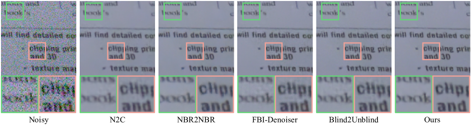
Figure 3: Visualization results on one typical image of the SIDD Benchmark.

Noise Type	Method	BSD68	Set12	Urabn100
$\alpha=0.01$ $\sigma=0.0002$	Baseline, N2C [34]	30.82/0.877	31.49/0.881	30.80/0.901
	Baseline, N2N [25]	30.76/0.876	31.47/0.880	30.84/0.900
	GAT+BM3D [13]	30.08/0.849	30.36/0.871	30.44/0.881
	N2V [22]	29.04/0.824	29.29/0.830	27.48/0.830
	FBI-D [8]	28.09/0.784	29.13/0.828	27.28/0.829
	NBR2NBR [20]	30.38/0.861	31.07/0.869	30.15/0.884
	Blind2Unblind [36]	30.61/0.869	31.45/0.880	30.70/0.900
	Ours	30.83/0.875	31.68/0.886	31.14/0.908
$\alpha=0.01$ $\sigma=0.02$	Baseline, N2C [34]	30.54/0.868	31.26/0.876	30.51/0.892
	Baseline, N2N [25]	30.62/0.871	31.34/0.878	30.70/0.899
	GAT+BM3D [13]	29.86/0.844	30.55/0.857	30.23/0.882
	N2V [22]	29.01/0.828	29.43/0.842	27.53/0.838
	FBI-D [8]	27.95/0.776	29.11/0.824	27.21/0.822
	NBR2NBR [20]	30.28/0.860	31.00/0.868	30.15/0.886
	Blind2Unblind [36]	30.41/0.865	31.27/0.877	30.49/0.896
	Ours	30.62/0.869	31.47/0.880	30.91/0.902
$\alpha=0.05$ $\sigma=0.02$	Baseline, N2C [34]	27.11/0.765	27.78/0.801	26.69/0.813
	Baseline, N2N [25]	27.07/0.762	27.71/0.799	26.58/0.808
	GAT+BM3D [13]	26.16/0.732	27.26/0.785	26.40/0.795
	N2V [22]	26.25/0.719	26.48/0.755	24.71/0.741
	FBI-D [8]	25.75/0.683	26.42/0.745	24.51/0.722
	NBR2NBR [20]	26.88/0.751	27.51/0.783	26.39/0.800
	Blind2Unblind [36]	27.02/0.757	27.65/0.796	26.54/0.805
	Ours	27.17/0.766	27.96/0.805	26.96/0.819

Table 2: Grayscale image denoising results. Bold and underlined are the highest and second without supervision.

5.3 Results for Synthetic Denoising

Grayscale Denoising  The denoising results on synthetic grayscale images are presented in Table 2. Three Poisson-Gaussian noise levels are simulated to evaluate the performance of the proposed method under low, medium, and high Poisson-Gaussian noise levels. The results show that our approach outperforms several denoising methods, including the traditional denoising method GAT+BM3D and four self-supervised denoising methods (N2V, NBR2NBR, FBI-D, and Blind2Unblind) for both low and high Poisson-Gaussian noise levels. In addition, our method outperforms two supervised baselines (N2C and N2N) on Set12 and Urban100, with a maximum gain of 0.4 dB, and performs competitively on BSD68. These results highlight the superior generalization of our method on grayscale image denoising compared to supervised baselines. Compared with the recent best Blind2Unblind, our method has a maximum gain of 0.44 dB and a minimum gain of 0.15 dB, demonstrating the necessity of explicit personalized denoising.

Noise Type	Method	KODAK	SET14	BSD300
$\alpha=0.01$ $\sigma=0.0002$	Baseline, N2C [34]	34.67/0.925	33.16/0.904	33.61/0.929
	Baseline, N2N [25]	34.64/0.924	33.13/0.904	33.59/0.928
	GAT+BM3D [13]	33.63/0.913	31.80/0.883	32.47/0.909
	N2V [22]	31.68/0.871	30.72/0.848	29.71/0.844
	FBI-D [8]	31.66/0.871	30.66/0.848	29.69/0.843
	NBR2NBR [20]	34.10/0.918	32.69/0.896	32.89/0.919
	Blind2Unblind [36]	33.88/0.915	32.47/0.886	32.53/0.913
	Ours	34.23/0.920	32.75/0.896	33.00/0.921
$\alpha=0.01$ $\sigma=0.02$	Baseline, N2C [34]	34.39/0.920	32.93/0.899	33.28/0.923
	Baseline, N2N [25]	34.36/0.920	32.89/0.899	33.25/0.923
	GAT+BM3D [13]	33.39/0.909	31.58/0.876	32.21/0.904
	N2V [22]	31.51/0.867	30.56/0.845	29.55/0.838
	FBI-D [8]	31.54/0.867	30.56/0.846	29.58/0.838
	NBR2NBR [20]	33.93/0.915	32.52/0.892	32.87/0.916
	Blind2Unblind [36]	33.58/0.909	32.17/0.883	32.31/0.910
	Ours	34.12/0.917	32.60/0.893	32.95/0.917
$\alpha=0.05$ $\sigma=0.02$	Baseline, N2C [34]	30.80/0.854	29.69/0.837	29.45/0.843
	Baseline, N2N [25]	30.77/0.853	29.65/0.836	29.43/0.842
	GAT+BM3D [13]	29.19/0.824	27.58/0.801	27.87/0.799
	N2V [22]	29.03/0.793	28.14/0.785	27.42/0.759
	FBI-D [8]	29.15/0.800	28.29/0.791	27.48/0.763
	NBR2NBR [20]	30.49/0.848	29.46/0.832	29.20/0.837
	Blind2Unblind [36]	30.58/0.849	29.52/0.832	29.27/0.837
	Ours	30.69/0.850	29.57/0.833	29.33/0.838

Table 3: PSNR(dB)/SSIM on synthetic sRGB datasets.

sRGB Denoising  The results of synthetic denoising for sRGB images are presented in Table 3. Our method outperforms GAT+CBM3D and four self-supervised methods (N2V, NBR2NBR, FBI-D, and Blind2Unblind) in both low and high noise levels. However, the gain over Blind2Unblind decreases at high noise levels due to numerous missing details valuable for restoring clean signals. Unlike grayscale denoising in Table 2, our method does not outperform supervised baselines in sRGB denoising but achieves competitive performance at high noise levels. Intuitively, cross-channel correlation makes noise removal in sRGB space more challenging than in grayscale images. As the noise level increases, the necessity for clean target supervision gradually decreases. Moreover, we observe that Blind2Unblind with greedy pixel-level objective outperforms NBR2NBR with neighboring approximation at high noise levels, highlighting the potential of lossless denoising for high noise levels.

Methods	SIDD			FMD
	RAW	RAW	sRGB	Confocal	Two-Photon
	Benchmark	Validation	Benchmark	Mice	Mice
Baseline, N2C [34]	50.61/0.991	51.19/0.991	38.08/0.945	38.40/0.966	34.02/0.925
Baseline, N2N [25]	50.62/0.991	51.21/0.991	38.09/0.945	38.37/0.965	33.80/0.923
GAT+BM3D [13]	48.60/0.986	48.92/0.986	34.64/0.879	37.93/0.963	33.83/0.924
N2V [22]	48.01/0.983	48.55/0.984	34.21/0.864	37.49/0.960	33.38/0.916
DBSN [37]	49.56/0.987	50.13/0.988	36.77/0.917	30.61/0.730	26.24/0.423
BP-AIDE [9]	50.45/0.990	–	37.91/0.942	38.31/0.963	33.89/0.902
FBI-D [8]	50.57/0.990	–	38.07/0.942	38.32/0.963	33.95/0.908
NBR2NBR [20]	50.47/0.990	51.06/0.991	37.85/0.942	37.07/0.960	33.40/0.921
Blind2Unblind [36]	50.79/0.991	51.36/0.992	38.11/0.944	38.44/0.964	34.03/0.916
Ours	50.92/0.991	51.50/0.992	38.21/0.945	38.46/0.965	34.11/0.918

Table 4: PSNR(dB)/SSIM on SIDD and FMD dataset.

5.4 Results for Real-World Denoising

Table 4 shows the quantitative results for the SIDD benchmark and validation datasets in raw-RGB and sRGB space. The proposed Blind2Sound outperforms all self-supervised methods and supervised baselines, showcasing its strong generalization ability for real-world scenarios with various dynamic Poisson-Gaussian noise levels. Notably, our method achieves a gain of nearly 0.3 dB over FBI-D in raw-RGB space, validating the effectiveness of lossless denoising. Blind2Sound outperforms Blind2Unblind with a gain of 0.1 dB, confirming the importance of explicit personalized modeling. The visual results in Figure 3 demonstrate that Blind2Sound restores the highest level of texture details and pixel correlation while avoiding bad artifacts. In contrast, Blind2Unblind displays visible clumping shadows in multiple regions due to insufficient denoising. Even supervised baselines show notable artifacts under dynamic noise, further validating the superiority of noise-sensed personalized denoising. The denoising results on FMD dataset indicate that Blind2Sound outperforms self-supervised methods and has competitive performance compared to supervised baselines.

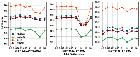
Figure 4: Ablation study on Cramer Gaussian loss with fixed weight $1$ for $L_{arv}$ and horizontal is the weight of $L_{est}$.

5.5 Ablation Study

This section presents ablation studies on various factors, including grain size, Cramer Gaussian loss, training scheme, noise model, re-visible correlation and visible factor. PSNR(dB)/SSIM is evaluated on CBSD68 while training on CBSD432 for 200 epochs.

Ablation study on grain size. Table 5 shows that fine-grained sub-block constraints improve the accuracy of the coarse-grained Gaussian loss, enhance robustness, and reduce solution space to provide more accurate noise parameters. However, smaller sub-block sizes results in limited noise context, leading to lower performance.

Ablation study on Cramer Gaussian loss. As shown in Figure 4, the denoiser with a weight of $0.01$ performs best compared to $0$ or $100$. Joint optimization can restore more image details and actual noise levels of optimal denoised images may differ from raw noisy images. Hence, Cramer Gaussian loss only serves as a regularization to assist the denoiser in sensing the most suitable noise level.

Ablation study on training scheme. As shown in Table 6, $T+J$ performs better than $T+P$ and $T+F$ at low noise, but they are comparable at high noise. At low noise, $T+P$ and $T+F$ mismatch the actual noise levels of restored images, thus degrading performance. At high noise, three training schemes estimate almost identical noise parameters.

Ablation study on noise model. Table 7 shows that $\mathcal{M}_{E}$ performs slightly better than the other noise models at low noise, but much better at high noise. $\mathcal{M}_{O}$ amplifies Poisson noise error in masked branch due to signal dependence, while $\mathcal{M}_{S}$ violates the independence of two branches.

Ablation study on re-visible correlation. Table 8 explores the impact of whether masked and visible branches are independent. The denoiser in the IID setting performs much better than in the non-IID setting. IID decouples the correlation between the blind and visible branches, thus achieving visible denoising without mask suppression.

Ablation study on visible factor. Table 9 shows the performance using different visible factors. The degree of visible is not proportional to the performance. Instead, the performance first increases and then decreases as the visible factor increases, reaching a peak when $\lambda_{f}=11$.

Grain Size	$(0.01,0.0002)$	$(0.01,0.02)$	$(0.05,0.02)$	$(0.1,0.02)$
CG	0.007/0.038	0.009/0.034	0.039/0.057	0.092/0.039
FG1	0.010/0.011	0.010/0.021	0.046/0.021	0.089/0.008
CG+FG1	0.010/0.012	0.010/0.021	0.048/0.022	0.093/0.019
CG+FG2	0.009/0.008	0.010/0.022	0.043/0.027	0.085/0.013
CG+FG1+FG2	0.009/0.009	0.010/0.022	0.046/0.024	0.092/0.017

Table 5: Ablation study on grain size for BSD68. CG is global coarse grain, FG1 is four sub-blocks each in three-quarter size and FG2 is nine sub-blocks in one-half size.

Training Scheme	$(0.01,0.0002)$	$(0.01,0.02)$	$(0.05,0.02)$
$T+P$	32.78/0.914	32.69/0.913	29.24/0.838
$T+F$	33.02/0.917	32.70/0.913	29.26/0.839
$T+J$	33.14/0.920	32.89/0.916	29.29/0.840

Table 6: Ablation study on training scheme, $T+P$, $T+F$ and $T+J$ represent training using frozen pre-trained noise estimator, training with fixed true noise or joint training.

Loss Type	$(0.01,0.0002)$	$(0.01,0.02)$	$(0.05,0.02)$
$\mathcal{M}_{O}$	33.11/0.919	32.84/0.913	29.12/0.833
$\mathcal{M}_{S}$	33.10/0.919	32.86/0.915	29.14/0.835
$\mathcal{M}_{E}$	33.14/0.920	32.89/0.916	29.29/0.840

Table 7: Ablation study on noise model. $\mathcal{M}_{O}$ and $\mathcal{M}_{E}$ denote Eq. 13 and Eq. 14. $\mathcal{M}_{S}$ means $diag(\alpha\boldsymbol{\mu_{y}})+\sigma\boldsymbol{\rm{I}}$.

Loss Type	$(0.01,0.0002)$	$(0.01,0.02)$	$(0.05,0.02)$
non-IID	32.19/0.904	32.24/0.905	28.95/0.827
IID	33.14/0.920	32.89/0.916	29.29/0.840

Table 8: Ablation study on re-visible correlation. non-IID and IID indicate whether the masked and visible branches are independent.

Noise Type	$\lambda_{f}=3$	$\lambda_{f}=11$	$\lambda_{f}=20$	$\lambda_{f}=40$
$(0.01,0.0002)$	33.05/0.919	33.14/0.920	33.11/0.920	33.06/0.919
$(0.01,0.02)$	32.75/0.914	32.89/0.916	32.84/0.915	32.76/0.914
$(0.05,0.02)$	29.24/0.838	29.29/0.840	29.27/0.839	29.23/0.837

Table 9: Ablation study on visible factor. Note that the initial value $\lambda_{s}=3$ and $\lambda_{f}$ is the final value.

6 Conclusion

We propose Blind2Sound, a self-supervised blind denoising framework that removes Poisson-Gaussian noise without residual noise and adapts to sensed noise levels. Adaptive re-visible loss associates noise parameters with re-visible transitions to achieve personalized and lossless denoising. Cramer Gaussian loss introduces fine-grained noise knowledge to improve estimation accuracy. The noise estimator is removed during inference. Extensive experiments show that our approach achieves superior performance, especially in real scenes with dynamic noise.

References

- [1] Abdelrahman Abdelhamed. Website. https://www.eecs.yorku.ca/~kamel/sidd/benchmark.php. Accessed: 2018-11-01.
- [2] Abdelrahman Abdelhamed, Stephen Lin, and Michael S Brown. A high-quality denoising dataset for smartphone cameras. In CVPR, pages 1692–1700, 2018.
- [3] Francis J Anscombe. The transformation of poisson, binomial and negative-binomial data. Biometrika, 35(3/4):246–254, 1948.
- [4] Saeed Anwar and Nick Barnes. Real image denoising with feature attention. In ICCV, pages 3155–3164, 2019.
- [5] Joshua Batson and Loic Royer. Noise2self: Blind denoising by self-supervision. In ICML, pages 524–533, 2019.
- [6] Paul A Bromiley. Products and convolutions of gaussian distributions. Medical School, Univ. Manchester, Manchester, UK, Tech. Rep, 3:2003, 2003.
- [7] Tim Brooks, Ben Mildenhall, Tianfan Xue, Jiawen Chen, Dillon Sharlet, and Jonathan T Barron. Unprocessing images for learned raw denoising. In CVPR, pages 11036–11045, 2019.
- [8] Jaeseok Byun, Sungmin Cha, and Taesup Moon. Fbi-denoiser: Fast blind image denoiser for poisson-gaussian noise. In CVPR, pages 5768–5777, 2021.
- [9] Jaeseok Byun and Taesup Moon. Learning blind pixelwise affine image denoiser with single noisy images. SPL, 27:1105–1109, 2020.
- [10] Sungmin Cha and Taesup Moon. Fully convolutional pixel adaptive image denoiser. In ICCV, pages 4160–4169, 2019.
- [11] Guangyong Chen, Fengyuan Zhu, and Pheng Ann Heng. An efficient statistical method for image noise level estimation. In ICCV, pages 477–485, 2015.
- [12] Jingwen Chen, Jiawei Chen, Hongyang Chao, and Ming Yang. Image blind denoising with generative adversarial network based noise modeling. In CVPR, pages 3155–3164, 2018.
- [13] Kostadin Dabov, Alessandro Foi, Vladimir Katkovnik, and Karen Egiazarian. Image denoising by sparse 3-d transform-domain collaborative filtering. TIP, 16(8):2080–2095, 2007.
- [14] Jia Deng, Wei Dong, Richard Socher, Li-Jia Li, Kai Li, and Li Fei-Fei. Imagenet: A large-scale hierarchical image database. In CVPR, pages 248–255, 2009.
- [15] Alessandro Foi, Mejdi Trimeche, Vladimir Katkovnik, and Karen Egiazarian. Practical poissonian-gaussian noise modeling and fitting for single-image raw-data. TIP, 17(10):1737–1754, 2008.
- [16] Rich Franzen. Kodak lossless true color image suite. source: http://r0k. us/graphics/kodak, 4(2), 1999.
- [17] Shi Guo, Zifei Yan, Kai Zhang, Wangmeng Zuo, and Lei Zhang. Toward convolutional blind denoising of real photographs. In CVPR, pages 1712–1722, 2019.
- [18] Samuel W Hasinoff. Photon, poisson noise. Computer Vision: A Reference Guide, pages 608–610, 2014.
- [19] Jia-Bin Huang, Abhishek Singh, and Narendra Ahuja. Single image super-resolution from transformed self-exemplars. In CVPR, pages 5197–5206, 2015.
- [20] Tao Huang, Songjiang Li, Xu Jia, Huchuan Lu, and Jianzhuang Liu. Neighbor2neighbor: Self-supervised denoising from single noisy images. In CVPR, pages 14781–14790, 2021.
- [21] Diederik P Kingma and Jimmy Ba. Adam: A method for stochastic optimization. In ICLR, 2015.
- [22] Alexander Krull, Tim-Oliver Buchholz, and Florian Jug. Noise2void-learning denoising from single noisy images. In CVPR, pages 2129–2137, 2019.
- [23] Samuli Laine, Tero Karras, Jaakko Lehtinen, and Timo Aila. High-quality self-supervised deep image denoising. NeurIPS, 32:6970–6980, 2019.
- [24] Wooseok Lee, Sanghyun Son, and Kyoung Mu Lee. Ap-bsn: Self-supervised denoising for real-world images via asymmetric pd and blind-spot network. In CVPR, pages 17725–17734, 2022.
- [25] Jaakko Lehtinen, Jacob Munkberg, Jon Hasselgren, Samuli Laine, Tero Karras, Miika Aittala, and Timo Aila. Noise2noise: Learning image restoration without clean data. In ICML, 2018.
- [26] Xinhao Liu, Masayuki Tanaka, and Masatoshi Okutomi. Single-image noise level estimation for blind denoising. TIP, 22(12):5226–5237, 2013.
- [27] Xinhao Liu, Masayuki Tanaka, and Masatoshi Okutomi. Practical signal-dependent noise parameter estimation from a single noisy image. TIP, 23(10):4361–4371, 2014.
- [28] Markku Makitalo and Alessandro Foi. Optimal inversion of the generalized anscombe transformation for poisson-gaussian noise. TIP, 22(1):91–103, 2012.
- [29] David Martin, Charless Fowlkes, Doron Tal, and Jitendra Malik. A database of human segmented natural images and its application to evaluating segmentation algorithms and measuring ecological statistics. In ICCV, volume 2, pages 416–423, 2001.
- [30] Nick Moran, Dan Schmidt, Yu Zhong, and Patrick Coady. Noisier2noise: Learning to denoise from unpaired noisy data. In CVPR, pages 12064–12072, 2020.
- [31] Tongyao Pang, Huan Zheng, Yuhui Quan, and Hui Ji. Recorrupted-to-recorrupted: Unsupervised deep learning for image denoising. In CVPR, pages 2043–2052, 2021.
- [32] Adam Paszke, Sam Gross, Francisco Massa, Adam Lerer, James Bradbury, Gregory Chanan, Trevor Killeen, Zeming Lin, Natalia Gimelshein, Luca Antiga, et al. Pytorch: An imperative style, high-performance deep learning library. NeurIPS, 32:8026–8037, 2019.
- [33] Stanislav Pyatykh, Jürgen Hesser, and Lei Zheng. Image noise level estimation by principal component analysis. TIP, 22(2):687–699, 2012.
- [34] Olaf Ronneberger, Philipp Fischer, and Thomas Brox. U-net: Convolutional networks for biomedical image segmentation. In International Conference on Medical image computing and computer-assisted intervention, pages 234–241, 2015.
- [35] Stefan Roth and Michael J Black. Fields of experts: A framework for learning image priors. In CVPR, volume 2, pages 860–867. IEEE, 2005.
- [36] Zejin Wang, Jiazheng Liu, Guoqing Li, and Hua Han. Blind2unblind: Self-supervised image denoising with visible blind spots. In CVPR, 2022.
- [37] Xiaohe Wu, Ming Liu, Yue Cao, Dongwei Ren, and Wangmeng Zuo. Unpaired learning of deep image denoising. In ECCV, pages 352–368, 2020.
- [38] Jun Xu, Yuan Huang, Ming-Ming Cheng, Li Liu, Fan Zhu, Zhou Xu, and Ling Shao. Noisy-as-clean: learning self-supervised denoising from corrupted image. TIP, 29:9316–9329, 2020.
- [39] Zongsheng Yue, Hongwei Yong, Qian Zhao, Deyu Meng, and Lei Zhang. Variational denoising network: Toward blind noise modeling and removal. NeurIPS, 32:1690–1701, 2019.
- [40] Syed Waqas Zamir, Aditya Arora, Salman Khan, Munawar Hayat, Fahad Shahbaz Khan, Ming-Hsuan Yang, and Ling Shao. Cycleisp: Real image restoration via improved data synthesis. In CVPR, pages 2696–2705, 2020.
- [41] Syed Waqas Zamir, Aditya Arora, Salman Khan, Munawar Hayat, Fahad Shahbaz Khan, Ming-Hsuan Yang, and Ling Shao. Learning enriched features for real image restoration and enhancement. In ECCV, pages 492–511, 2020.
- [42] Roman Zeyde, Michael Elad, and Matan Protter. On single image scale-up using sparse-representations. In International conference on curves and surfaces, pages 711–730, 2010.
- [43] Kai Zhang, Wangmeng Zuo, Yunjin Chen, Deyu Meng, and Lei Zhang. Beyond a gaussian denoiser: Residual learning of deep cnn for image denoising. TIP, 26(7):3142–3155, 2017.
- [44] Kai Zhang, Wangmeng Zuo, and Lei Zhang. Ffdnet: Toward a fast and flexible solution for cnn-based image denoising. TIP, 27(9):4608–4622, 2018.
- [45] Yide Zhang, Yinhao Zhu, Evan Nichols, Qingfei Wang, Siyuan Zhang, Cody Smith, and Scott Howard. A poisson-gaussian denoising dataset with real fluorescence microscopy images. In CVPR, 2019.