A Theory for Semantic Channel Coding With Many-to-one Source

Abstract

As one of the potential key technologies of 6G, semantic communication is still in its infancy and there are many open problems, such as semantic entropy definition and semantic channel coding theory. To address these challenges, we investigate semantic information measures and semantic channel coding theorem. Specifically, we propose a semantic entropy definition as the uncertainty in the semantic interpretation of random variable symbols in the context of knowledge bases, which can be transformed into existing semantic entropy definitions under given conditions. Moreover, different from traditional communications, semantic communications can achieve accurate transmission of semantic information under a non-zero bit error rate. Based on this property, we derive a semantic channel coding theorem for a typical semantic communication with many-to-one source (i.e., multiple source sequences express the same meaning), and prove its achievability and converse based on a generalized Fano’s inequality. Finally, numerical results verify the effectiveness of the proposed semantic entropy and semantic channel coding theorem.

I Introduction

According to the classic information theory established by Claude Shannon in 1948 [1], communication systems advances are made by exploring new spectrum utilization methods and new coding schemes. However, due to the explosive growth of intelligent services, such as augmented reality/virtual reality, holographic communication, and autonomous driving [2, 3, 4], the fifth generation communications (5G) system is facing many bottlenecks: channel capacity is approaching Shannon limit [5, 6, 7], source coding efficiency is close to the Shannon information entropy/rate distortion function limit [8], the energy consumption is huge [9], and high-quality spectrum resources are scarce [10]. To meet the development needs of future sixth generation communications (6G), there is an urgent need for new information representation space and degrees of freedom to improve communication efficiency and transmission capacity.

Semantic communications [11, 12] extract semantic features from raw data, then encode and transmit semantic information, which are expected to alleviate the bottlenecks faced by the current communication networks [7, 13]. Back in 1949, Weaver proposed a three-level communication theory [14] as follows, Back in 1949, Weaver proposed a three-level communication theory [14] as follows,

• Technical level: How accurately can the symbols of communication be transmitted?

• Semantic level: How precisely do the transmitted symbols convey the desired meaning?

• Effectiveness level: How effectively does the received meaning affect conduct in the desired way?

Essentially, semantic communications reduce communication resource overhead, i.e., bandwidth, power consumption or delay, by exploiting computing power, which focuses on the accurate transmission of semantic information. Furthermore, semantic communications transform traditional grammatical communications into content-oriented communications, which will be one of the key technologies of 6G communications [15, 16, 17, 18].

I-A Related works

Recently, with the great progress of artificial intelligence (AI), neural networks can extract semantic information, such as images, text, and speech, which makes semantic communications feasible [19, 20, 21]. However, there are still many open problems in semantic communications, especially lacking information metrics and theoretic guidelines to implement and analyze semantic communications. [22, 23].

To measure the quantity of semantic information for a source, many works proposed semantic entropy based on logical probability [24, 25, 26], fuzzy mathematics theory[27, 28], language understanding model[29] or the complexity of query tasks[30] Specifically, in 1952, Carnap and Bar-Hillel [24] used propositional logic probability instead of statistical probability to measure the semantic information contained in a sentence, that is, the higher the probability of a sentence being logically true, the less semantic information it contains. The amount of semantic information [25] was represented based on the distance from the real event, which needs the “true” semantic event as a reference. With background knowledge, the semantic entropy of messages is defined based on propositional logic theory [26]. A semantic entropy definition was proposed based on fuzzy mathematics theory by [27]. According to the membership degree in fuzzy set theory, the authors in [28] defined the semantic entropy for classification tasks, which is used to calculate the optimal semantic description for each category. In [29], the semantic entropy was derived based on the general structure in the language understanding model. Based on the complexity of query tasks, the semantic entropy was defined as the minimum number of semantic queries for data query tasks[30]. Besides, a multi-grained definition of semantic information was proposed in [31] for different levels of communication systems, and used Rényi entropy [32] to measure semantic information. Semantic information was defined as grammatical information [33] describing the relationship between the system and its environment. The existing semantic entropy definitions are based on the specific tasks, and there are significant differences between different definitions of semantic entropy, which makes it difficult to extend them to other applications.

Besides, in contrast to traditional communications, semantic communications can achieve accurate transmission of semantic information with a non-zero bit error rate. However, how to establish semantic channel capacity is still a challenge issue, and some works tried to prove the achievability of the semantic channel capacity. The “semantic channel capacity” was derived based on the semantic ambiguity and the logical semantic entropy of the received signal by [34]. However, a typical joint error between the wrong codeword and the received sequence [35] was ignored in [34] and there is no proof of the converse. The authors in [36] modeled semantic communication as a Bayesian game problem, which minimized the semantic error by optimizing the sending strategy. In [8] a semantic communication rate-distortion framework was proposed to characterize semantic distortion and signal distortion. Semantic communication was modeled as a signaling game model in game theory [37], and described conditional mutual information based on semantic knowledge base. In summary, semantic channel capacity, as the rate limit on which a channel can accurately transmit semantic information, is still an open problem.

I-B Contributions

With the above motivations, we propose a more general definition of semantic entropy with the help of Shannon information entropy and prove the semantic channel coding theorem for a typical semantic communications. Specifically, the main contributions of this paper are summarized as follows:

• The existing semantic entropy definitions are task-oriented, which limits its generalizability. To address this issue, we adopt the a more general definition of semantic entropy as the uncertainty in the semantic interpretation of random variable symbols in the context of knowledge bases. Our proposed semantic entropy definition not only depends on the probability distribution, but also depends on the specific value of the symbol and the background knowledge base. Different from the traditional measure of information, our proposed semantic entropy has two unique features: on the one hand, semantic information has a certain degree of ambiguity, that is, different symbols can express the same semantic meaning; on the other hand, the same symbol may have different semantic meanings under different knowledge bases. Under the given conditions, semantic entropy can be transformed into existing semantic entropy definitions.

• Furthermore, we establish a semantic channel coding theorem for semantic communications with “many-to-one” semantic source, i.e., multiple source sequences express the same meaning. We first prove its achievability based on the jointly typicality tools and many-to-one mapping relation. We then prove the converse based on a generalized Fano’s inequality. To our best knowledge, it is the first time theoretically established the fundamental limits of semantic communications with many-to-one semantic source. This provides a theoretical tool for the semantic communication design.

• Simulation results verify the feasibility and effectiveness of our proposed semantic entropy, and prove that with a non-zero bit error rate, the accuracy of the classification task is still high, which verifies the rationality of our proposed semantic channel coding theorem.

TABLE I: Summary of Key Notations

Notations	Meanings
$X,Y$	Random variables
$x,y$	Values of random variables
${{S}}$	The semantic interpretation of random variable $X$
${\text{Pr}}\left(\cdot\right)$	The probability of “$\cdot$” occurs
${{\cal X}}$, ${{\cal Y}}$	The finite sets
${\left\lceil{\alpha nR}\right\rceil}$	The smallest integer not less than ${\alpha nR}$
$m$	The index of the message set with the same semantic
$x^{n}$, $y^{n}$	$n$-length sequences
$X^{n}$, $Y^{n}$	$n$-length sequences of random variables
${{\cal X}^{n}}$, ${{\cal Y}^{n}}$	The sequence sets of $X^{n}$, $Y^{n}$
$\varepsilon$	An error message
$\emptyset$	Null set
$\left|\cdot\right|$	The number of containing elements

TABLE II: The relationships between our proposed semantic entropy, the existing semantic entropy definitions and Shannon entropy.

Forms	Semantic entropy equation	Relationship with the proposed semantic entropy
Proposed semantic entropy	${H_{s}}\left(X\right)=-\sum\limits_{{s}}{p\left({{s}}\right){{\log}_{2}}p\left({{s}}\right)}$	$/$
Logical semantic entropy[26]	$H\left(M\right)=-\sum\limits_{m\in{\Delta_{M}}}{{P_{M}}\left(m\right){{\log}_{2}}\left({{P_{M}}\left(m\right)}\right)}$	$p\left({{s}}\right)={p_{M}}\left(m\right)$ is logical probability
Fuzzy semantic entropy[28]	$H\left(\zeta\right)=-\sum\limits_{j=1}^{m}{{D_{j}}\left(\zeta\right){{\log}_{2}}{D_{j}}\left(\zeta\right)}$	$p\left({{s}}\right)={D_{j}}\left(\zeta\right)$ is the degree of match
Language understanding semantic entropy [29]	$H\left({{v_{t}}}\right)=-\sum\limits_{{{\mathbf{v}}_{M}}\in{V_{\mathcal{M}}}}{P\left({{{\mathbf{v}}_{M}}|{{\mathbf{v}}_{t}}}\right)\log P\left({{{\mathbf{v}}_{M}}|{{\mathbf{v}}_{t}}}\right)}$	$p\left({{s}}\right)=p\left({{{\mathbf{v}}_{M}}|{{\mathbf{v}}_{t}}}\right)$ is the conditional probability of language understanding
Shannon entropy [35]	$H\left(X\right)=-\sum\limits_{x\in\mathcal{X}}{p\left(x\right)\log p\left(x\right)}$	${p\left(x\right)}$ is the probability mass function

The rest of this paper is organized as follows. We propose a definition of semantic entropy in Section II. We propose a semantic channel coding theorem and prove its achievability in Section III. In Section IV, we derive and prove the generalized Fano’s inequality and use it to prove the converse of the semantic channel coding theorem. Finally, Section V concludes the paper. Table I presents the key notations in this paper and their meanings.

II General Definition of Semantic Entropy

Shannon entropy is a functional of the distribution of a random variable, which does not depend on the actual states taken by the random variable, but only on their probabilities. As a result, Shannon entropy can not be directly applied to measure the semantic information. Different from Shannon information theory, semantic information has the following two characteristics:

• The semantic has a certain degree of ambiguity. That is, different symbols can express the same meaning. For example, “red” and “crimson” both mean “red” in the given knowledge base condition.

• The semantic meaning of the symbol may be different under a different knowledge base. For instance, “notebook” indicates paper notebook in stationery store and also means computer in computer store. It depends on the specific context knowledge base.

Consequencely, semantic entropy of a random variable depends not only on its probability distribution, but also on the value of the random variable and its background knowledge base.

Note that, the existing semantic entropy definitions are task-oriented, that is, these semantic entropies can only be used in the given tasks. To propose a more general measure of semantic information, we define the semantic entropy as the uncertainty of the semantic interpretation of the random variable in the knowledge base background.

II-A Discrete semantic entropy

Specifically, let $X$ denote a discrete random variable with the probability mass function ${p}\left(x\right)$. Based on knowledge base $\mathcal{K}$, let ${{S}}$ denote the semantic interpretation of the discrete random variable $X$. The semantic interpretation ${{S}}$ depends on the value of $X$ and knowledge base $\mathcal{K}$. Furthermore, the probability mass function of the semantic interpretation ${{S}}$ is given as,

$$p\left({{s}}\right)=\sum_{x}\limits{p_{\mathcal{K}}\left({{s}|x}\right)p\left(x\right)},$$ (1)

where the conditional probability $p_{\mathcal{K}}\left({{s}|x}\right)$ is the probability transition function from random variable $X$ to its semantic interpretation ${{S}}$, which depends on the value of $X$ and knowledge base $\mathcal{K}$. Sometimes, it is difficult to measure the relationship $p\left({{s}|x}\right)$ between random variable $X$ and its semantic ${{S}}$. Estimating $p\left({{s}|x}\right)$ is a challenging problem, and one could use statistical methods or deep learning (DL) to estimate.

Definition 1.

The discrete semantic entropy ${H_{\text{s}}}\left(X\right)$ of the random variable $X$ given knowledge base $\mathcal{K}$ is defined by,

$${H_{\text{s}}}\left(X\right) \triangleq-\sum\limits_{{s}}{\big{(}\sum_{x}\limits{p_{\mathcal{K}}\left({{s}|x}\right)p\left(x\right)}\big{)}{{\log}_{2}}\big{(}\sum_{x}\limits{p_{\mathcal{K}}\left({{s}|x}\right)p\left(x\right)}\big{)}}.$$ (2)

The relationships between our proposed semantic entropy and the existing semantic entropy definitions and Shannon entropy are shown in Table II.

The following two examples illustrate the relationship between semantic entropy and its value and knowledge base.

Example 1. The random variable $X\in\mathcal{X}$ represents the student mentioned by the teacher, its value space $\mathcal{X}$ has three different values, $\mathcal{X}=\left\{{{x_{1}}:{\text{Alice}},{x_{2}}:{\text{Bob}},{x_{3}}:{\text{Cindy}}}\right\}$. Assume the probability of ${x_{i}}$ is shown in Table III. Then, the Shannon entropy of random variable $X$ is $H\left(X\right)=1.5{\text{bits}}$.

TABLE III: the probability of ${x_{i}}$.

$X$	${x_{1}}$	${x_{2}}$	${x_{3}}$
$p\left({{x_{i}}}\right)$	$0.25$	$0.5$	$0.25$

Example 2. Given the knowledge base $\mathcal{K}$, let ${S}$ denote the semantic interpretation of the random variable $X$ in Example 1, its semantic interpretation space $\mathcal{S}=\left\{{{s_{n}}}\right\}_{n=1}^{N}$, ${S}\in{\mathcal{S}}$. The transition probability from $X$ to ${S}$ is written as $p\left({{s_{n}}\left|{{x_{i}}}\right.}\right)={\Pr_{{\mathcal{K}}}}\left({{S}={s_{n}}|X={x_{i}}}\right)$.

TABLE IV: The transition probability from $X$ to ${S}$.

Condition		${x_{1}}$	${x_{2}}$	${x_{3}}$
$\mathcal{K}_{1}$	${s_{1}}$	$\frac{1}{3}$	$\frac{1}{3}$	$\frac{1}{3}$
	${s_{2}}$	$\frac{1}{3}$	$\frac{1}{3}$	$\frac{1}{3}$
	${s_{3}}$	$\frac{1}{3}$	$\frac{1}{3}$	$\frac{1}{3}$
$\mathcal{K}_{2}$	${s_{1}}$	$\frac{9}{10}$	$\frac{4}{5}$	$\frac{1}{2}$
	${s_{2}}$	$\frac{1}{10}$	$\frac{1}{5}$	$\frac{1}{2}$

(1) Based on knowledge base ${\mathcal{K}_{1}}$: physical education class. Semantic interpretation ${S}$ indicates the instruction that the mentioned student needs to complete, and semantic interpretation space ${\mathcal{S}_{1}}=\left\{{{s_{1}}{\text{: Turn left, }}{s_{2}}{\text{: Go straight, }}{s_{3}}{\text{: Turn right}}}\right\}$ and ${S}\in{\mathcal{S}_{1}}$. The corresponding transition probabilities ${p_{1}}\left({{s_{n}}|{x_{i}}}\right)$ are listed in Table IV. According to (1), the probabilities of the corresponding semantic interpretation are calculated as ${p_{1}}\left({{s_{n}}}\right)=\Pr\left({{S}={s_{n}}}\right)=\frac{1}{3},n=1,2,3$. Thus, with the knowledge base ${\mathcal{K}_{1}}$, the semantic entropy of $X$ is ${H_{{{\text{s}}_{\text{1}}}}}\left(X\right)=-\sum\limits_{{s_{n}}}{{p_{1}}\left({{s_{n}}}\right){{\log}_{2}}{p_{1}}\left({{s_{n}}}\right)}={\log_{2}}3\left({{\text{bits}}}\right)$, which is larger than its Shannon entropy $H\left(X\right)=1.5({\text{bits}})$.

(2) Based on knowledge base ${\mathcal{K}_{2}}$: the classroom. Semantic interpretation ${S}$ indicates the willingness of the student being questioned. The semantic space ${\mathcal{S}_{2}}=\left\{{{s_{1}}:{\text{Agree}},{s_{2}}:{\text{Disagree}}}\right\}$, ${S}\in{\mathcal{S}_{2}}$. The corresponding transition probabilities ${p_{2}}\left({{s_{n}}|{x_{i}}}\right)$ are listed in Table IV. Hence, ${p_{2}}\left({{s_{1}}}\right)=\frac{3}{4}$ and ${p_{2}}\left({{s_{2}}}\right)=\frac{1}{4}$. Further, with the knowledge base ${\mathcal{K}_{2}}$, the semantic entropy of $X$ is ${H_{{{\text{s}}_{\text{2}}}}}\left(X\right)=-\sum\limits_{{s_{n}}}{{p_{2}}\left({{s_{n}}}\right){{\log}_{2}}{p_{2}}\left({{s_{n}}}\right)}=2-\frac{3}{4}{\text{lo}}{{\text{g}}_{\text{2}}}{\text{3}}\left({{\text{bits}}}\right)$, which is lower than its Shannon entropy $H\left(X\right)=1.5({\text{bits}})$.

Since the semantic information of $X$ relies on the distribution $p\left({{s}}\right)$, the proposed discrete semantic entropy ${H_{\text{s}}}\left(X\right)$ of $X$ may be higher, lower than or equal to Shannon entropy $H\left(X\right)$.

II-B Differential semantic entropy

Let $S$ denote the semantic random variable of the symbol $X$ with probability density function $f\left(w\right)$, and the corresponding mapping function is, The semantic interpretation depends on the value of $X$ and knowledge base $\mathcal{K}$. Furthermore, the probability density function of the semantic interpretation $S$ is given as,

$$f\left(s\right)=\int_{x}{f\left({s|x}\right)f\left(x\right)dx},$$ (3)

where $f\left({s|x}\right)$ is the probability transition function from random variable $X$ to its semantic interpretation $S$, which depends on the value of $X$ and knowledge base $\mathcal{K}$. Thus, the differential semantic entropy ${h_{\text{s}}}\left(X\right)$ of the symbol $X$ is defined as,

$${h_{\text{s}}}\left(X\right)\triangleq h\left(S\right)=-\int\limits_{s}{f\left(s\right){{\log}_{2}}f\left(s\right)ds}.$$ (4)

II-C Measure of semantic knowledge

Let $K$ represent the semantic knowledge variable with probability distribution $p\left({k}\right)$. Thus, the entropy of semantic knowledge $K$ is given as,

$$H\left(K\right)=-\sum\limits_{k}{p\left({k}\right){{\log}_{2}}p\left({k}\right)}.$$ (5)

It is well known that semantic coding can provide extremely high compression ratios, but the specific measure of semantic compression is still unknown. Next, we will try to explain the reasons for the high compression ratio of semantic encoding. The relationships among the random variables $X$, its semantic interpretation $S$, and semantic knowledge $K$ are given as,

$$H\left(X\right) ={I\left(K;X\right)}+{I\left(S;X|K\right)}+{H\left({X\left|{K,S}\right.}\right)}.$$

$$={I\left(K;X\right)}+{H(S|K)}-H\left(S|X,K\right)+{H\left({X\left|{K,S}\right.}\right)}.$$

where $I\left(K;X\right)$ represents the shared related knowledge between the transmitter and destination; $H(S|K)$ represents the conditional semantic entropy given the knowledge variable $K$, equaling to the semantic entropy $H(S)$ if $S$ and $K$ are independent; $H\left({X\left|{K,S}\right.}\right)$ represents the remaining information after extracting $K,S$.

Furthermore, let ${G_{\text{s}}}$ denote semantic compression gain, i.e., the ratio between Shannon entropy and semantic entropy of the data, w.t,

$${G_{\text{s}}}=\frac{{H\left(X\right)}}{{H\left(S\right)}}.$$ (7)

Thus, the amount of transmission will be decreased with the increase of semantic compression gain ${G_{\text{s}}}$. Since the transmitter and receiver share semantic knowledge, and semantic coding removes semantic redundancy, semantic communications has a high compression ratio. Our goal is to find the maximum achievable compression gain without semantic error.

Example 3. (Task-oriented semantic communication) Consider a typical task-oriented semantic communication system, i.e., the classification task for the MNIST dataset with a set of handwritten character numbers from 0 to 9. The semantic entropy of each image is equal to the Shannon entropy of labels, i.e., ${\log_{2}}10{\text{ bits}}$. The average size of each image of the MNIST dataset is about $6272{\text{ bits}}$. Therefore, its achievable semantic compression gain ${G_{\text{s}}}$ is given as,

$${G_{\text{s}}}=\frac{{6272}}{{{{\log}_{2}}10}}\approx 1888.$$ (8)

Example 4. (Data reconstruction semantic communication) Consider a typical data reconstruction semantic communication system with fourier transform (FT) and inverse fourier transform (IFT). Specifically, the semantic encoder and decoder are designed by FT and IFT, respectively.

Assume that the input signal is a single-frequency sine wave, i.e., $f\left(t\right)=\sin{\Omega_{0}}t$, and the amount of information are $N{\text{ bits}}$ bits (Since the number of discrete points in the time domain may tend to be infinite, the value of N may tend to be infinite).

Via the FT-based semantic encoder, the frequency domain expression of the input signal is given as,

$$F\left(\Omega\right)=j\pi\left[{\delta\left({\Omega+{\Omega_{0}}}\right)-\delta\left({\Omega-{\Omega_{0}}}\right)}\right].$$ (9)

Note that ${\Omega_{0}}\in{\omega_{0}}$ is the semantic information, and the semantic entropy is $\operatorname{H}\left({{\Omega_{0}}}\right)=\sum\limits_{{\Omega_{0}}\in{\omega_{0}}}{-p\left({{\Omega_{0}}}\right)}$ ${\log_{2}}p\left({{\Omega_{0}}}\right)$ bits. Generally, $\operatorname{H}\left({{\Omega_{0}}}\right)$ is a limited value. The parameters $j$, $\pi$ and $\delta\left(\Omega\right)$ is the semantic knowledge base shared by the transmitter and receiver. Therefore, the semantic compression gain is ${G_{\text{s}}}=\frac{N}{{\operatorname{H}\left({{\Omega_{0}}}\right)}}$, which may tend to infinity.

III Semantic channel coding theorem

III-A Semantic communication system model

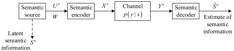
Figure 1:  A semantic communication system

Consider a semantic communication system, as depicted in Fig. 1. Assume that the source sequence ${U^{n}}$ and semantic information sequence ${S^{n}}$ satisfy the “many-to-one” mapping relations. Specifically, as shown in Fig. 2, $\mathcal{U}$ and $\mathcal{S}$ denote the source sequence set and the semantic sequence set, respectively, and $u_{l}^{n}$ and $s_{t}^{n}$ denote the $l$-th source sequence in $\mathcal{U}$ and $t$-th semantic sequence in $\mathcal{S}$, respectively, where $l\in\left\{{1,\ldots,L}\right\}$ and $t\in\left\{{1,\ldots,T}\right\}$. Moreover, ${\mathcal{U}_{{s_{t}}}}$ is the set of source sequences has the same semantic meaning $s_{t}^{n}$. Furthermore, the corresponding transition probability $\sum\limits_{s}{p\left({{s^{n}}\left|{{u^{n}}}\right.}\right)=1}$ for all $u^{n}\in\mathcal{U}_{s}$, where $\mathcal{U}_{s}$ denotes the set of source sequences has the same semantic meaning $s^{n}$. Define a message $W\in\left[{1:{2^{n\operatorname{H}\left(U\right)}}}\right]$ with a “one-to-one” correspondence to the source $U$. The semantic transmitter wishes to reliably transmit the latent semantic information $S$ within the message $W$ at a rate $R$ bits per transmission to the semantic receiver over a noisy physical channel.

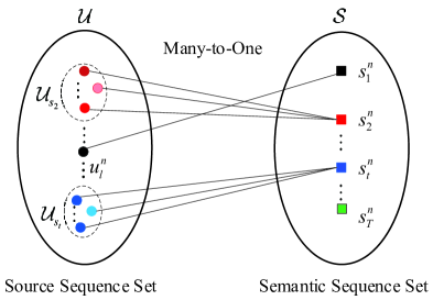
Figure 2:  The “many-to-one” relations between ${U^{n}}$ and ${S^{n}}$.

Toward this end, the semantic transmitter encodes the message $W$ into a codeword $X^{n}$ and transmits it over the channel in $n$ time channel uses. Upon receiving the noisy sequence $Y^{n}$, the semantic receiver decodes it to obtain the estimate $\widehat{S}$ of the semantic message. The semantic channel coding problem is concerned with finding the highest rate $R$ such that the probability of semantic decoding error can be made to decay asymptotically to zero with the code block length $n$.

Consider the sematic channel coding problem for a typical discrete memoryless channel (DMC) model $p\left({y|x}\right)$ with a finite input set ${\mathcal{X}}$ and a finite output set ${\mathcal{Y}}$.

The source message set $\left[{{\text{1}}:{2^{nR}}}\right]=\left\{{{\text{1}},{\text{2}},...,{2^{nR}}}\right\}$ consists a semantic message set $\left[{{\text{1}}:{2^{\left\lceil{\alpha nR}\right\rceil}}}\right]$ $=\left\{{{\text{1}},{\text{2}},...,{2^{\left\lceil{\alpha nR}\right\rceil}}}\right\}$, where the coefficient $\alpha$ lies in the range $0\leq\alpha<1$.

A semantic encoder assigns a codeword ${X^{n}}\left(m\right)$ to message $W\in\left[{{\rm{1:}}{2^{nR}}}\right]$, where $m\in\left[{1:{2^{\alpha nR}}}\right]$ is the index of the message set with the same semantic meaning. Furthermore, let ${\Phi_{m}}$ denote the subset of message $W$ with the same semantic information, $m\in\left[{1:{2^{\alpha nR}}}\right]$, where ${\Phi_{m}}$ satisfies ${\Phi_{m}}\subseteq\left[{{\rm{1:}}{2^{nR}}}\right]$, ${\Phi_{m}}\cap{\Phi_{l}}=\emptyset,\forall m\neq l$ and $\bigcup\nolimits_{m=1}^{{2^{\alpha nR}}}{{\Phi_{m}}=\left[{{\rm{1:}}{2^{nR}}}\right]}$. Then, a semantic decoder assigns an estimate $\widehat{m}\in\left[{1:{2^{\alpha nR}}}\right]$ or an error message $\varepsilon$ to each received sequence ${Y^{n}}$, ${\mathcal{Y}^{n}}\in\left[{{\rm{1:}}{2^{\alpha nR}}}\right]\cup\left\{\varepsilon\right\}$. We assume that the semantic message is uniformly distributed over the message set $\left[{1:{2^{\alpha nR}}}\right]$.

The performance of a given code is measured by the probability that the estimate of the semantic message is different from the actual semantic message sent. The set $\mathcal{C}=\left\{{{x^{n}}\left(1\right),{x^{n}}\left(2\right),\ldots,}\right.$ $\left.{{x^{n}}\left({{2^{\left\lceil{\alpha nR}\right\rceil}}}\right)}\right\}$is referred to as the codebook associated with the $\left({{2^{\alpha nR}},n}\right)$ code. More precisely, let ${\lambda_{m}}\left({\cal C}\right)={\rm{Pr}}\left\{{\widehat{S}\neq m|S=m}\right\}$ be the conditional probability of error given semantic index $m$ is sent. Then, the average probability of error for a $\left({{2^{\alpha nR}},n}\right)$ code is,

$$P_{{\text{e,s}}}^{\left(n\right)}\left(\mathcal{C}\right)={\text{Pr}}\left\{{\widehat{S}\neq S}\right\}=\frac{1}{{{2^{\left\lceil{\alpha nR}\right\rceil}}}}\sum\limits_{m=1}^{{2^{\left\lceil{\alpha nR}\right\rceil}}}{{{\text{E}}_{\mathcal{C}}}\left({{\lambda_{m}}\left(\mathcal{C}\right)}\right)}.$$ (10)

III-B Semantic channel coding theorem

Given the semantic mapping ${f_{s}}:\left[{1:{2^{nR}}}\right]\to\left[{1:{2^{\alpha nR}}}\right]$ and the discrete memoryless channel $p\left({y\left|x\right.}\right)$, we define the semantic channel capacity ${C_{\text{s}}}$ as

$${C_{\text{s}}}=\mathop{\max}\limits_{p\left(x\right)}\frac{{I\left({X;Y}\right)}}{\alpha}.$$ (11)

Theorem 1.

Semantic channel coding theorem: For every bit rate $R<{C_{\text{s}}}={\max_{p\left(x\right)}}\frac{{I\left({X;Y}\right)}}{\alpha}$, there exists a sequence of $\left({{2^{nR}},n}\right)$ codes with average probability of error $P_{{\text{e,s}}}^{\left(n\right)}$ that tends to zero as $n\to\infty$.
Conversely, for every sequence of $\left({{2^{nR}},n}\right)$ codes with probability of error $P_{{\text{e,s}}}^{\left(n\right)}$ that tends to zero as $n\to\infty$, the rate must satisfy $R<{C_{\text{s}}}={\max_{p\left(x\right)}}\frac{{I\left({X;Y}\right)}}{\alpha}$.

Note that, different form the proof of Shannon channel coding theorem, the semantic information mapping should be incorporated in both semantic encoding and decoding in the achievability proof of proposed semantic coding theorem. We first prove the achievability in the following subsection. The proof of the converse is given in Section IV. B

Proof.

For simplicity of presentation, we assume throughout the proof that $nR$, $\alpha nR$ and $n{R_{\text{s}}}$ are integers.

Semantic source: Given a source message $W\in\left[{{\rm{1:}}{2^{nR}}}\right]$. Let $S$ represent the inherent semantic information of $W$. Let ${f_{\text{s}}}:\left[{1:{2^{nR}}}\right]\to\left[{1:{2^{\alpha nR}}}\right]$ represent the semantic mapping from $W$ to $S$.

Random codebook generation: By applying random coding, we randomly and independently generate ${2^{n{R_{\text{s}}}}}$ sequences ${x^{n}}\left(m\right)$, each according to $p\left({{x^{n}}}\right)=\prod\limits_{i=1}^{n}{{p_{X}}\left({{x_{i}}}\right)}$. The generated sequences constitute the codebook $\mathcal{C}=\left[{{\rm{1:}}{2^{n{R_{\text{s}}}}}}\right]$ as follows

$$p\left(\mathcal{C}\right)=\prod\limits_{m=1}^{{2^{n{R_{\text{s}}}}}}{\prod\limits_{i=1}^{n}{{p_{X}}\left({{x_{i}}\left(m\right)}\right)}}.$$ (12)

The codebook $\mathcal{C}$ is known by both the semantic encoder and the semantic decoder. In order to represent ${2^{\alpha nR}}$ semantic information losslessly, ${R_{\text{s}}}$ must satisfy

$${R_{\text{s}}}\geq\alpha R.$$ (13)

Semantic encoding: Given a source message ${W}$, the encoder finds the corresponding semantic information set index $m$, i.e., to send semantic index $m\in\left[{1:{2^{n{R_{\text{s}}}}}}\right]$, and transmits ${x^{n}}\left(m\right)$.

Semantic decoding: Let ${y^{n}}$ be the received sequence. The receiver declares that $\widehat{m}$ is sent if ${x^{n}}\left({\widehat{m}}\right)$ and ${y^{n}}$ are jointly typical; otherwise, if there is none or more than one such message, it declares an error $\mathcal{E}$.

Analysis of the probability of error: Assume that the sending semantic index $m$ obeys a uniform distribution on $m\in\left[{1:{2^{n{R_{\text{s}}}}}}\right]$. Without loss of generality, we assume that semantic index $m=1$ is sent and typical sequence ${x^{n}}\left(1\right)$ is sent, received as ${y^{n}}$, and thus the decoder makes an error if $\left({{x^{n}}\left(1\right),{y^{n}}}\right)$ are not jointly typical. Let $\mathcal{E}=\left\{{\widehat{m}\neq m}\right\}$ denote the semantic error event. Consider the probability of semantic errors averaged over all codewords and codebooks, we have

$${\text{Pr}}\left(\mathcal{E}\right) ={{\rm E}_{\mathcal{C}}}\left({P_{{\text{e,s}}}^{\left(n\right)}}\right)$$ (14a)

$$={{\rm E}_{\mathcal{C}}}\left({\frac{1}{{{2^{n{R_{\text{s}}}}}}}\sum\limits_{m=1}^{{2^{n{R_{\text{s}}}}}}{{\lambda_{m}}\left(\mathcal{C}\right)}}\right)$$ (14b)

$$=\frac{1}{{{2^{n{R_{\text{s}}}}}}}\sum\limits_{m=1}^{{2^{n{R_{\text{s}}}}}}{{{\rm E}_{\mathcal{C}}}\left({{\lambda_{m}}\left(\mathcal{C}\right)}\right)}$$ (14c)

$$={{\rm E}_{\mathcal{C}}}\left({{\lambda_{1}}\left(\mathcal{C}\right)}\right)$$ (14d)

$$=\Pr\left({\mathcal{E}\left|{m=1}\right.}\right),$$ (14e)

where $\lambda_{m}$ is the conditional probability of semantic error given semantic index $m$ was sent. Equation (14d) holds due to the symmetry of the random codebook generation.

The decoder makes an error if one or both of the following events occur:

• $E_{1}^{c}$ is defined as $\left({{X^{n}}\left(1\right),{Y^{n}}}\right)$ not jointly typical;

• ${E_{m}}$ is defined as $\left({{X^{n}}\left(m\right),{Y^{n}}}\right)$ semantic jointly typical, where $m\neq 1$.

Thus, by the union of events bound

$${\text{Pr}}\left(\mathcal{E}\right) =P\left({E_{1}^{c}\cup{{\left\{{{E_{m}}}\right\}}_{m\neq 1}}}\right)$$ (15a)

$$\leq P\left({E_{1}^{c}}\right)+P\left({{{\left\{{{E_{m}}}\right\}}_{m\neq 1}}}\right)$$ (15b)

$$\leq\varepsilon+\sum\limits_{m\neq 1}{P\left({{E_{m}}}\right)}$$ (15c)

$$\leq\varepsilon+\sum\limits_{m\neq 1}{{2^{-n\left({I\left({X;Y}\right)-3\varepsilon}\right)}}}$$ (15d)

$$=\varepsilon+\left({{2^{n{R_{\text{s}}}}}-1}\right){2^{-n\left({I\left({X;Y}\right)-3\varepsilon}\right)}}$$ (15e)

$$\leq\varepsilon+{2^{3n\varepsilon}}{2^{-n\left({I\left({X;Y}\right)-{R_{\text{s}}}}\right)}}$$ (15f)

$$\leq 2\varepsilon,$$ (15g)

where inequality (15b) holds due to the probabilities of union events bound, inequality (15c) holds due to $P\left({E_{1}^{c}}\right)\to 0$ as $n\to\infty$, inequality (15d) holds due to the jointly typical probability of ${X^{n}}\left(m\right)$ and ${Y^{n}}$ is no more than ${2^{-n\left({I\left({X;Y}\right)-3\varepsilon}\right)}}$, inequality (15e) holds due to $\left({{2^{n{R_{\text{s}}}}}-1}\right)\to{2^{n{R_{\text{s}}}}}$ as $n\to\infty$, and inequality (15g) holds because ${R_{\text{s}}}\leq I\left({X;Y}\right)$.

Furthermore, by combining ${R_{\text{s}}}\geq\alpha R$ and ${R_{\text{s}}}\leq I\left({X;Y}\right)$, we can obtain

$$R\leq\frac{{I\left({X;Y}\right)}}{\alpha}.$$ (16)

Hence, there exists a sequence of $\left({{2^{nR}},n}\right)$ codes such that ${\lim_{n\to\infty}}P_{{\text{e,s}}}^{\left(n\right)}=0$, which proves that $R<{C_{\text{s}}}={\max_{p\left(x\right)}}\frac{{I\left({X;Y}\right)}}{\alpha}$ is achievable. Finally, taking $\varepsilon\to 0$ completes the proof. ∎

IV Converse Proof

Fano’s inequality is the key to proving the converse of the channel coding theorem [35]. However, since different symbols may have the same semantic information, the traditional bit error judgment rule cannot be directly used for semantic symbol error judgment, which makes Fano’s inequality not applicable to semantic communications.

IV-A Extended Fano’s inequality

To prove the converse of the semantic channel coding theorem, we first derive and prove the semantic Fano’s inequality. Specifically, the message $W$ is uniformly distributed on the set $\left[{{\rm{1:}}{2^{nR}}}\right]\triangleq\Psi$, $W\in\Psi$ and the sequence ${Y^{n}}$ is related probabilistically to $W$. From ${Y^{n}}$, we estimate that the message $W$ was sent. Let the estimate be $\widehat{W}=g\left({{Y^{n}}}\right)$. Thus, $W\to{X^{n}}\left(W\right)\to{Y^{n}}\to\widehat{W}$ forms a Markov chain. Define the semantic error probability $P_{{\text{e,s}}}^{\left(n\right)}\triangleq\Pr\left\{{\widehat{W}\notin{\Phi_{W}}}\right\}$. For semantic communication systems, assume that the number of messages with the same semantic information as $W$ is ${2^{\left({1-\alpha}\right)nR}}=\beta\left|\Psi\right|$, and the set of messages is denoted as ${\Phi_{W}}$, $\left|{{\Phi_{W}}}\right|={2^{\left({1-\alpha}\right)nR}}$, where $\alpha$ and $\beta$ are coefficients which satisfy $0\leq\alpha<1$, $0\leq\beta<1$, respectively.

Theorem 2.

Semantic Fano’s inequality: Given message $W\in\left[{{\rm{1:}}{2^{nR}}}\right]$ with semantic $\left[{1:{2^{nR}}}\right]\to\left[{1:{2^{\alpha nR}}}\right]$. Let $P_{{\text{e,s}}}^{\left(n\right)}=\Pr\left\{{\widehat{W}\notin{\Phi_{W}}}\right\}$, we have

$$H\left({W|{Y^{n}}}\right)\leq 1+\left({1-\alpha+\left({\gamma+\alpha-1}\right)P_{{\text{e,s}}}^{\left(n\right)}}\right)nR.$$ (17)

Proof.

Define a semantic error random variable $E$ as follows

$$E=\left\{\begin{gathered}\begin{array}[]{*{20}{c}}1&{{\text{if }}\widehat{W}\notin{\Phi_{W}}}\end{array}\hfill\\ \begin{array}[]{*{20}{c}}0&{{\text{if }}\widehat{W}\in{\Phi_{W}}}\end{array}\hfill\\ \end{gathered}\right..$$ (23)

Then, by applying the chain rule for entropies to expand $H\left({E,W|{Y^{n}}}\right)$ in two different ways, we have

$$H\left({E,W|{Y^{n}}}\right) =H\left({W|{Y^{n}}}\right)+H\left({E|W,{Y^{n}}}\right)$$ (24a)

$$=H\left({E|{Y^{n}}}\right)+H\left({W|E,{Y^{n}}}\right).$$ (24b)

Because conditioning reduces entropy, $H\left({E|{Y^{n}}}\right)\leq H\left(E\right)$. Moreover, due to $E$ being a function of $W$ and ${Y^{n}}$, the conditional entropy $H\left({E|W,{Y^{n}}}\right)=0$. Furthermore, since $E$ is a binary-valued random variable, $H\left(E\right)\leq 1$. Thus, $H\left({W|E,{Y^{n}}}\right)$ is bounded as follows

$$H\left({W|E,{Y^{n}}}\right)= \Pr\left({E=0}\right)H\left({W|{Y^{n}},E=0}\right)$$

$$+\Pr\left({E=1}\right)H\left({W|{Y^{n}},E=1}\right)$$ (25a)

$$\leq \left({1-P_{{\text{e,s}}}^{\left(n\right)}}\right){\log_{2}}\left({\beta\left|\Psi\right|}\right)$$

$$+P_{{\text{e,s}}}^{\left(n\right)}{\log_{2}}\left({\left({1-\beta}\right)\left|\Psi\right|}\right)$$ (25b)

$$= \left({1-P_{{\text{e,s}}}^{\left(n\right)}}\right)\left({1-\alpha}\right)nR+P_{{\text{e,s}}}^{\left(n\right)}\gamma nR$$ (25c)

$$= \left({1-\alpha+\left({\gamma+\alpha-1}\right)P_{{\text{e,s}}}^{\left(n\right)}}\right)nR,$$ (25d)

where $\gamma\triangleq\frac{1}{{nR}}{\log_{2}}\left({1-\beta}\right)+1$, inequality (25b) holds since $E=0$, $\widehat{W}\in{\Phi_{W}}$ and $E=1$, $\widehat{W}\notin{\Phi_{W}}$. The upper bound on the conditional entropy is the log of the number of possible outcomes of $W$. Combining these results, we obtain the semantic Fano inequality (17). ∎

IV-B Converse to semantic channel coding theorem

To prove the converse to the channel coding theorem, we need to show that for every sequence of $\left({{2^{nR}},n}\right)$ codes with ${\lim_{n\to\infty}}P_{{\text{e,s}}}^{\left(n\right)}=0$, we must have $R<{C_{\text{s}}}={\max_{p\left(x\right)}}\frac{{I\left({X;Y}\right)}}{\alpha}$.

Proof.

For a given semantic encoding ${X^{n}}\left(\cdot\right)$ and a given semantic decoding rule $\widehat{W}=g\left({{Y^{n}}}\right)$, we have $W\to{X^{n}}\left(W\right)\to{Y^{n}}\to\widehat{W}$. For each $n$, let $W$ be drawn according to a uniform distribution over $\left[{{\rm{1:}}{2^{nR}}}\right]$. Define $P_{{\text{e,s}}}^{\left(n\right)}=\Pr\left\{{\widehat{W}\notin{\Phi_{W}}}\right\}$, hence, we have

$$nR= H\left(W\right)$$ (26a)

$$= H\left({W|{Y^{n}}}\right)+I\left({W;{Y^{n}}}\right)$$ (26b)

$$\leq H\left({W|{Y^{n}}}\right)+I\left({{X^{n}}\left(W\right);{Y^{n}}}\right)$$ (26c)

$$\leq 1+\left({1-\alpha+\left({\gamma+\alpha-1}\right)P_{{\text{e,s}}}^{\left(n\right)}}\right)nR$$

$$+I\left({{X^{n}}\left(W\right);{Y^{n}}}\right)$$ (26d)

$$\leq 1+\left({1-\alpha+\left({\gamma+\alpha-1}\right)P_{{\text{e,s}}}^{\left(n\right)}}\right)nR+n{C},$$ (26e)

where (26a) holds due to the assumption that $W$ is uniform over $\left[{{\rm{1:}}{2^{nR}}}\right]$, inequality (26c) holds due to the data-processing inequality, inequality (26d) holds due to semantic Fano’s inequality, and inequality (26d) holds due to $I\left({{X^{n}}\left(W\right);{Y^{n}}}\right)\leq n{C}$. Dividing by $n$, we obtain

$$R\leq \frac{1}{{\left({\alpha-\left({\gamma+\alpha-1}\right)P_{{\text{e,s}}}^{\left(n\right)}}\right)n}}+\frac{I\left({X;Y}\right)}{{\alpha-\left({\gamma+\alpha-1}\right)P_{{\text{e,s}}}^{\left(n\right)}}}.$$ (27)

Now letting $n\to\infty$ and $P_{{\text{e,s}}}^{\left(n\right)}\to 0$, and hence

$$R\leq\frac{I\left({X;Y}\right)}{\alpha}.$$ (28)

As a result, for every sequence of $\left({{2^{nR}},n}\right)$ codes with ${\lim_{n\to\infty}}P_{{\text{e,s}}}^{\left(n\right)}=0$, we must have $R<{C_{\text{s}}}={\max_{p\left(x\right)}}\frac{{I\left({X;Y}\right)}}{\alpha}$, which completes the proof of the converse. ∎

V Experiments and Discussions

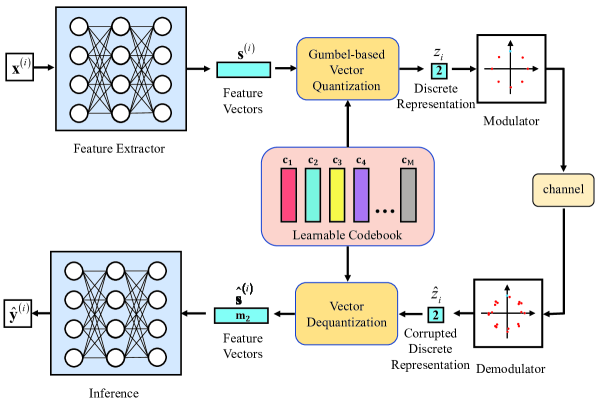
Figure 3:   A task-oriented semantic communication system.

According to the proposed definition of general semantic entropy, the interpretation of the semantic variable of the classification task is the category. Therefore, the source semantic entropy of the classification task is the Shannon entropy of the category. In order to further verify the effectiveness of the definition of semantic entropy and rationality of the proposed semantic channel coding theorem, we adopt a classification task-oriented semantic communication system [38] with the MNIST dataset. As is shown in Fig. 3, based on the DL network, the feature extractor first extracts feature vectors from the input image. Furthermore, according to the shared learnable codebook, the Gumbel-based vector quantization converts the extracted feature vectors into discrete representations, and then performs digital modulation and sends it to the receiver. The receiver first demodulates the received signal to corrupted discrete representations, and further performs vector dequantization to obtain feature vectors. Finally, the feature vectors are decoded by DL-based inference network, and output the classification information.

V-1 Semantic entropy verification

Assuming that the number of categories of input images is $N$, and thus the source semantic entropy is ${\log_{2}}N$. Moreover, we adopt $M$-PSK digital modulation scheme.

In order to verify the effectiveness of semantic entropy, we first consider the semantic source coding, ignoring the channel noise, that is, the DL-based encoder network and the DL-based decoder network are jointly trained under the noise-free channel condition.

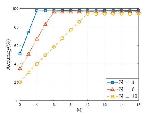
Figure 4:   Performance of the MNIST $N$-classification task

Fig. 4 shows the relationship between receiver inference accuracy performance and modulation order $M$-PSK with input image categories $N=4,6,10$. From the Fig. 4, it can be observed that when the modulation order $M$ is smaller than the number of input image categories $N$, the inference accuracy increases as the modulation order $M$ increases, because as $M$ increases, the modulated bits can represent more source semantic information; when $M\geq N$, the inference accuracy reaches $95\%$ and remains unchanged, because the semantic information of the information source is fully represented by the modulated bits. Therefore, Fig. 4 verifies that the source semantic entropy are ${\log_{2}}N$ bits.

Fig. 5 (a) and (b) shows the inference performance of classification task for the MNIST dataset under different SNRs with $N=6$ and $10$, respectively. From Fig. 5 (a) and (b), we observe that the inference accuracy increases first and then remains constant as the SNR increases. When the modulation order $M$ is smaller than $N$, the inference accuracy is lower than $90\%$ even at high SNR. In particular, for the high SNR, when the modulation order $M$ increases to $N$, the inference accuracy will be significantly improved, and the inference accuracy will not increase with the increase of $M$. Fig. 5 (a) and (b) verify that the semantic entropy of the classification task is equal to the Shannon entropy of the category.

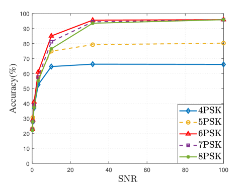
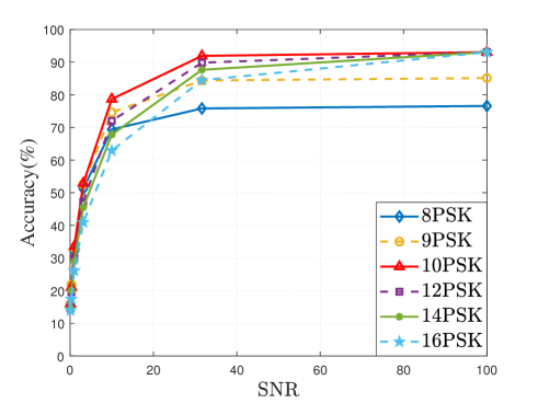
Figure 5: (a) the inference performance of 6-classification task and (b) the inference performance of 10-classification task.

V-2 Semantic channel coding theorem verification

Since complex Gaussian noise is utilized in the adopted model, the channel capacity $C={\log_{2}}\left({1+{\text{SNR}}}\right)$. We already know the average size of each image of the MNIST dataset is about $6272{\text{ bits}}$. It can be seen from Fig. 5 (a) and (b) that when the SNR is 63, the channel capacity is 6 bit/s, which is far less than the source entropy. However, when the modulation order $M\geq N$, the receiver can still achieve high inference accuracy. In addition, when the signal rate through the channel exceeds the channel capacity of Shannon theorem, the BER is significantly increased, and the information quality is seriously decreased. In fact, the channel capacity is only the limit that can be reached theoretically, and how to reach it in practice cannot be explained by the theorem. In Fig. 5 (b), we take 10PSK with N = 10 as an example, its transmission rate ${\text{R = }}{\log_{2}}10{\text{ bit/s}}$, when SNR is 9, the channel capacity ${\text{C = }}{\log_{2}}10{\text{ bit/s}}$, and the classification accuracy is about $75\%$. We also observe that $R>C$ from Fig. 5 (a) and (b), some images are still accurately classified and the accuracy is greater than the $\frac{1}{{10}}$ probability of blind guess. The above experiments verify the rationality of the proposed semantic channel coding theorem.

VI Conclusions

In this paper, we present a more general definition of semantic entropy and prove the semantic channel coding theorem for semantic communications. Different from existing definitions of semantic entropy which can only be applied to specific tasks, we define the semantic entropy as the uncertainty in the semantic interpretation of random variable symbols in the context of knowledge bases, which not only depends on the probability distribution, but also depends on the specific value of the symbol and the background knowledge base. Moreover, semantic entropy can be transformed into existing semantic entropy definitions and Shannon entropy. Furthermore, exploiting the fact that different bits can have the same semantic information, we first propose semantic channel coding theorem, and prove its achievability and converse. Our work attempts to provide fundamentals for the study of semantic communication.

References

- [1] C. E. Shannon, “A mathematical theory of communication,” ACM SIGMOBILE Mobile Comput. Commun. Rev., vol. 5, no. 1, pp. 3–55, 2001.
- [2] C. Anthes, R. J. García-Hernández, M. Wiedemann, and D. Kranzlmüller, “State of the art of virtual reality technology,” in IEEE Aerosp. conf., Jun. 2016, pp. 1–19.
- [3] A. Voulodimos, N. Doulamis, A. Doulamis, E. Protopapadakis et al., “Deep learning for computer vision: A brief review,” Comput. Intell. Neuroscience, Feb. 2018.
- [4] I. F. Akyildiz and H. Guo, “Holographic-type communication: A new challenge for the next decade,” ITU J. Future and Evolving Technologies., Sept. 2022.
- [5] K. Niu, J. Dai, and P. Zhang, “Semantic communication for 6G,” Mobile Commun., vol. 45, no. 04, pp. 85–90, Jul. 2021.
- [6] P. Zhang, W. Xu, H. Gao, K. Niu, X. Xu, X. Qin, C. Yuan, Z. Qin, H. Zhao, J. Wei et al., “Toward wisdom-evolutionary and primitive-concise 6G: A new paradigm of semantic communication networks,” Eng., vol. 8, pp. 60–73, Nov. 2021.
- [7] G. Shi, Y. Xiao, Y. Li, D. Gao, and X. Xie, “Semantic communication network for intelligent connection of all things,” Chin. J. Int. Things, vol. 5, no. 02, pp. 26–36, Apr. 2021.
- [8] J. Liu, W. Zhang, and H. V. Poor, “A rate-distortion framework for characterizing semantic information,” in IEEE Int. Symp. Inf. Theory (ISIT), Jul. 2021, pp. 2894–2899.
- [9] C.-X. Wang, M. D. Renzo, S. Stanczak, S. Wang, and E. G. Larsson, “Artificial intelligence enabled wireless networking for 5G and beyond: Recent advances and future challenges,” IEEE Wirel. Commun., vol. 27, no. 1, pp. 16–23, Feb. 2020.
- [10] W. Hong, C. Yu, J. Chen, and Z. Hao, “Millimeter wave and terahertz technology,” Sci. China: Inf. Sci., vol. 46, no. 8, pp. 1086–1107, 2016.
- [11] Y. Zhang, P. Zhang, Q. Wei, H. Zhao, J. Xiong, and J. Zhang, “Semantic communication for agents: Architecture and example,” Sc. China: Inf. Sci., vol. 52, no. 05, pp. 907–921, May. 2022.
- [12] W. Xu, Z. Yang, D. W. K. Ng, M. Levorato, Y. C. Eldar, and M. Debbah, “Edge learning for B5G networks with distributed signal processing: Semantic communication, edge computing, and wireless sensing,” IEEE J. Sel. Topics Signal Process., vol. 17, no. 1, pp. 9–39, Jan. 2023.
- [13] Q. Lan, D. Wen, Z. Zhang, Q. Zeng, X. Chen, P. Popovski, and K. Huang, “What is semantic communication? A view on conveying meaning in the era of machine intelligence,” J. Commun. Inf. Netw., vol. 6, no. 4, pp. 336–371, Dec. 2021.
- [14] C. E. Shannon and W. Weaver, “The mathematical theory of communication,” vol. 34, no. 310, 1950, pp. 312–313.
- [15] G. Shi, Y. Xiao, Y. Li, and X. Xie, “From semantic communication to semantic-aware networking: Model, architecture, and open problems,” IEEE Commun. Mag., vol. 59, no. 8, pp. 44–50, Aug. 2021.
- [16] E. C. Strinati and S. Barbarossa, “6G networks: Beyond shannon towards semantic and goal-oriented communications,” Comp. Netw., vol. 190, p. 107930, May. 2021.
- [17] L. Zhonghao, Z. Guangxu, X. Jie, A. Bo, and C. Shuguang, “Semantic communications for image recovery and classification via deep joint source and channel coding,” Apr. 2023.
- [18] Y. Shi, Y. Zhou, D. Wen, Y. Wu, C. Jiang, and K. B. Letaief, “Task-oriented communications for 6g: Vision, principles, and technologies,” IEEE Wireless Communications, vol. 30, no. 3, pp. 78–85, 2023.
- [19] H. Xie and Z. Qin, “A lite distributed semantic communication system for internet of things,” IEEE J. Sel. Areas Commun., vol. 39, no. 1, pp. 142–153, Jan. 2021.
- [20] J. Shao, Y. Mao, and J. Zhang, “Learning task-oriented communication for edge inference: An information bottleneck approach,” IEEE J. Sel. Areas Commun., vol. 40, no. 1, pp. 197–211, Jan. 2022.
- [21] X. Kang, B. Song, J. Guo, Z. Qin, and F. R. Yu, “Task-Oriented image transmission for scene classification in unmanned aerial systems,” IEEE Trans. on Commun., vol. 70, no. 8, pp. 5181–5192, Jun. 2022.
- [22] Z. Qin, X. Tao, J. Lu, and G. Y. Li, “Semantic communications: Principles and challenges,” arXiv preprint arXiv:2201.01389, Dec. 2021.
- [23] G. Xin and P. Fan, “EXK-SC: A semantic communication model based on information framework expansion and knowledge collision,” Entropy, vol. 24, no. 12, p. 1842, Oct. 2022.
- [24] R. Carnap, Y. Bar-Hillel et al., “An outline of a theory of semantic information,” 1952.
- [25] L. Floridi, “Outline of a theory of strongly semantic information,” Minds Mach., vol. 14, no. 2, pp. 197–221, May. 2004.
- [26] P. Basu, J. Bao, M. Dean, and J. Hendler, “Preserving quality of information by using semantic relationships,” IEEE Int. Conf. Pervasive Comput. Commun. Workshops, pp. 58–63, May. 2012.
- [27] A. DE LUCA and S. TERMINI, “A definition of a nonprobabilistic entropy in the setting of fuzzy sets theory,” Inf. Control, vol. 20, pp. 301–312, May. 1972.
- [28] X. Liu, W. Jia, W. Liu, and W. Pedrycz, “AFSSE: An interpretable classifier with axiomatic fuzzy set and semantic entropy,” IEEE Trans. Fuzzy Syst., vol. 28, no. 11, pp. 2825–2840, Oct. 2020.
- [29] N. J. Venhuizen, M. W. Crocker, and H. Brouwer, “Semantic entropy in language comprehension,” Entropy, vol. 21, no. 12, p. 1159, Nov. 2019.
- [30] A. Chattopadhyay, B. D. Haeffele, D. Geman, and R. Vidal, “Quantifying task complexity through generalized information measures,” Sept. 2020.
- [31] M. Kountouris and N. Pappas, “Semantics-Empowered communication for networked intelligent systems,” IEEE Commun. Mag., vol. 59, no. 6, pp. 96–102, Jan. 2021.
- [32] A. Rényi, “On measures of entropy and information,” in Proc. Berkeley Symp. Math. Statist. Probability, vol. 4, 1961, pp. 547–562.
- [33] A. Kolchinsky and D. H. Wolpert, “Semantic information, autonomous agency and non-equilibrium statistical physics,” Interface Focus, vol. 8, no. 6, p. 20180041, 2018.
- [34] J. Bao, P. Basu, M. Dean, C. Partridge, A. Swami, W. Leland, and J. A. Hendler, “Towards a theory of semantic communication,” in IEEE Netw. Sci. Workshop, Jun. 2011, pp. 110–117.
- [35] T. M. Cover, Elements of information theory. John Wiley & Sons, 1999.
- [36] B. Güler, A. Yener, and A. Swami, “The semantic communication game,” in IEEE Int. Conf. Commun., May. 2016, pp. 1–6.
- [37] “Semantic communication as a signaling game with correlated knowledge bases,” in IEEE Veh. Technol. Conf. (VTC2022-Fall), Jan. 2022.
- [38] S. Xie, S. Ma, M. Ding, Y. Shi, M. Tang, and Y. Wu, “Robust information bottleneck for task-oriented communication with digital modulation,” IEEE J. Sel. Areas Commun., pp. 1–15, Jun. 2023.