A Frame Decomposition of the Funk-Radon Transform

Abstract

The Funk-Radon transform assigns to a function defined on the unit sphere its integrals along all great circles of the sphere. In this paper, we consider a frame decomposition of the Funk-Radon transform, which is a flexible alternative to the singular value decomposition. In particular, we construct a novel frame decomposition based on trigonometric polynomials and show its application for the inversion of the Funk-Radon transform. Our theoretical findings are verified by numerical experiments, which also incorporate a regularization scheme.

1 Introduction

The Funk-Radon transform assigns to a function $f\colon\mathbb{S}^{2}\to\mathbb{C}$ defined on the two-dimensional unit sphere $\mathbb{S}^{2}\coloneqq\{\boldsymbol{\xi}\in\mathbb{R}^{3}:\left\lVert\boldsymbol{\xi}\right\rVert=1\}$ its integrals along all great circles of the sphere, i.e.,

$$Rf(\boldsymbol{\xi})\coloneqq\frac{1}{2\pi}\int_{\boldsymbol{\xi}^{\top}\boldsymbol{\eta}=0}f(\boldsymbol{\eta})\,\mathrm{d}\boldsymbol{\eta}\,,\qquad\forall\,\boldsymbol{\xi}\in\mathbb{S}^{2}\,,$$ (1)

where $\mathrm{d}\boldsymbol{\eta}$ denotes the arclength on the great circle perpendicular to $\boldsymbol{\xi}$. Tracing back to works of Funk [17] and Minkowski [36] in the early twentieth century, it is also known as Funk transform, Minkowski-Funk transform or spherical Radon transform. It has found applications in diffusion MRI [43, 49], radar imaging [52], Compton camera imaging [48], photoacoustic tomography [24], and geometric tomography [18, Chap. 4]. Besides analytic inversion formulas, e.g., [4, 17, 21, 28], the numerical reconstruction of functions given its Funk-Radon transform can be done using mollifier methods [34, 44], the eigenvalue decomposition [23], or discretization on the cubed sphere [5]. Generalizations have been developed for various non-central sections of the sphere [2, 39, 45, 46] or for derivatives [28, 42].

In this paper, we are interested in frame decompositions (FDs) of the Funk-Radon transform. Originally developed in the framework of wavelet-vaguelette decompositions [1, 10, 11, 14, 15, 31, 33] and then extended to biorthogonal curvelet and shearlet decompositions [6, 8], FDs are generalizations of the singular value decomposition (SVD) [12, 16, 25, 26, 27, 50]. In particular, they allow SVD-like decompositions of bounded linear operators also in those cases when the SVD itself is either unknown, its computation is infeasible, or its structure is unfavourable. More precisely, given a bounded linear operator $A\colon X\to Y$ between real or complex Hilbert spaces $X$ and $Y$, an FD of $A$ is a decomposition of the form

$$Ax=\sum_{k=1}^{\infty}\sigma_{k}\left\langle\,x,e_{k}\,\right\rangle_{X}\tilde{f}_{k}\,,\qquad\forall\,x\in X\,.$$ (2)

Here, the sets $\left\{e_{k}\right\}_{k\in\mathbb{N}}$ and $\left\{f_{k}\right\}_{k\in\mathbb{N}}$ form frames over $X$ and $Y$, respectively, and $\{\tilde{f}_{k}\}_{k\in\mathbb{N}}$ denotes the dual frame of the frame $\left\{f_{k}\right\}_{k\in\mathbb{N}}$; see Section 2 below. The main requirement on $e_{k}$ and $f_{k}$ is that they satisfy the quasi-singular relation

$$\overline{\sigma_{k}}\,e_{k}=\,A^{*}f_{k}\,,\qquad\forall\,k\in\mathbb{N}\,,$$ (3)

where $\overline{\sigma_{k}}$ denotes the complex conjugate of the coefficient $\sigma_{k}\in\mathbb{C}$ and $A^{*}$ the adjoint of $A$. Using the FD (2) it is possible to compute (approximate) solutions of the linear equation $Ax=y$, and to develop filter-based regularization schemes as for the SVD [12, 26, 27]. However, the question remains whether frames satisfying (3) can be found. While this is possible by geometric considerations for some examples [11, 14, 15, 25], an explicit construction “recipe” exists in case that $A$ satisfies the stability condition

$$c_{1}\left\lVert x\right\rVert_{X}\leq\left\lVert Ax\right\rVert_{Z}\leq c_{2}\left\lVert x\right\rVert_{X}\,,\qquad\forall\,x\in X\,,$$ (4)

for some constants $c_{1},c_{2}>0$ and a Hilbert space $Z\subseteq Y$. In this case, one can start with an arbitrary frame $\left\{f_{k}\right\}_{k\in\mathbb{N}}$ over $Y$ with the additional property

$$a_{1}\left\lVert y\right\rVert_{Z}^{2}\leq\sum_{k=1}^{\infty}\alpha_{k}^{2}\left|\left\langle\,y,f_{k}\,\right\rangle_{Y}\right|^{2}\leq a_{2}\left\lVert y\right\rVert_{Z}^{2}\,,\qquad\forall\,y\in Y\,,$$ (5)

for coefficients $0\neq\alpha_{k}\in\mathbb{R}$ and some constants $a_{1},a_{2}>0$. Then, one defines

$$e_{k}\coloneqq\alpha_{k}A^{*}f_{k}\,,\qquad$$

which results in a frame $\left\{e_{k}\right\}_{k\in\mathbb{N}}$ over $X$ which satisfies (3) with $\overline{\sigma_{k}}=1/\alpha_{k}$ [26]. In case that $Z$ and $Y$ are Sobolev spaces, frames $\left\{f_{k}\right\}_{k\in\mathbb{N}}$ satisfying (5) can often be found (e.g., orthonormal wavelets [9]), which has resulted in FDs of the classic Radon transform [26, 27]. On the other hand, while the Funk-Radon transform satisfies a stability property of the form (4), see Theorem 3.1 below, frames which satisfy (5) are more difficult to find. The standard candidate would be spherical harmonics, which, however, already are the eigenfunctions of the Funk-Radon transform, and thus offer no further insight.

Hence, in this paper we consider a different approach for constructing FDs, which was originally outlined in [26]. This approach is still based on the stability property (4), but instead of (5) it only requires that

$$\left\lVert y\right\rVert_{Y}\leq\left\lVert y\right\rVert_{Z}\,,\qquad\forall\,y\in Z\,,$$ (6)

that $Z\subseteq Y$ is a dense subspace of $Y$, and that the frame functions $f_{k}$ are elements of $Z$, i.e., $\left\lVert f_{k}\right\rVert_{Z}<\infty$. In this case, one can build an alternative FD of $A$ similar to (2), which can then be used to compute the (unique) solution of the linear operator equation $Ax=y$ for any $y$ in the range $\mathcal{R}(A)$ of $A$, and to develop stable reconstruction approaches in case of noisy data $y^{\delta}$.

The aim of this paper is to show that the above approach is applicable to the Funk-Radon transform. In particular, we construct an FD using trigonometric functions, which have the advantage of their fast computation outperforming spherical harmonics, cf. [35, 53]. For this, we first review some background on frames and FDs in Section 2. Then, in Section 3 we show that all required properties are satisfied for the Funk-Radon transform with a suitable choice of the functions $f_{k}$. Furthermore, we provide explicit expressions for the frame functions $e_{k}$, leading to an FD and a corresponding reconstruction formula. Finally, in Section 4 we consider the efficient implementation of our derived FD and evaluate its reconstruction quality on a number of numerical examples.

2 Background on Frames and Frame Decompositions

In this section, we review some background on frames and FDs, collected from the seminal works [7, 9] and the recent article [26], respectively.

Definition 1

A sequence $\{e_{k}\}_{k\in\mathbb{N}}$ in a Hilbert space $X$ is called a frame over $X$, if and only if there exist frame bounds $0<B_{1},B_{2}\in\mathbb{R}$ such that there holds

$$B_{1}\left\lVert x\right\rVert_{X}^{2}\leq\sum\limits_{k=1}^{\infty}\left|\left\langle\,x,e_{k}\,\right\rangle_{X}\right|^{2}\leq B_{2}\left\lVert x\right\rVert_{X}^{2}\,,\qquad\forall\,x\in X\,.$$ (7)

For a given frame $\{e_{k}\}_{k\in\mathbb{N}}$, one can consider the frame (analysis) operator $F$ and its adjoint (synthesis) operator $F^{*}$, which are given by

$$\begin{split}&F\,\colon\,X\to\ell_{2}(\mathbb{N})\,,\qquad x\mapsto\left(\left\langle\,x,e_{k}\,\right\rangle_{X}\right)_{k\in\mathbb{N}}\,,\\ &F^{*}\,\colon\,\ell_{2}(\mathbb{N})\to X\,,\qquad\left(a_{k}\right)_{k\in\mathbb{N}}\mapsto\sum\limits_{k=1}^{\infty}a_{k}e_{k}\,.\end{split}$$ (8)

Due to (7) there holds $\sqrt{B_{1}}\leq\left\lVert F\right\rVert=\left\lVert F^{*}\right\rVert\leq\sqrt{B_{2}}$. Furthermore, one can define

$$Sx\coloneqq F^{*}Fx=\sum\limits_{k=1}^{\infty}\left\langle\,x,e_{k}\,\right\rangle_{X}e_{k}\,,\qquad\text{and}\qquad\tilde{e}_{k}\coloneqq S^{-1}e_{k}\,.$$ (9)

Since $S$ is continuously invertible with $B_{1}I\leq S\leq B_{2}I$, the functions $\tilde{e}_{k}$ are well-defined, and the set $\{\tilde{e}_{k}\}_{k\in\mathbb{N}}$ forms a frame over $X$ with frame bounds $B_{2}^{-1},B_{1}^{-1}$ called the dual frame of $\{e_{k}\}_{k\in\mathbb{N}}$. Furthermore, it can be shown that

$$x=\sum\limits_{k=1}^{\infty}\left\langle\,x,\tilde{e}_{k}\,\right\rangle_{X}e_{k}=\sum\limits_{k=1}^{\infty}\left\langle\,x,e_{k}\,\right\rangle_{X}\tilde{e}_{k}\,,\qquad\forall\,x\in X\,.$$ (10)

In general, this decomposition is not unique, which is a key difference between frames and bases, but it can be understood as the “most economical” one [9].

Next, we consider FDs. For this, we use the following

Assumption 1

The operator $A\colon X\to Y$ between the Hilbert spaces $X,Y$ is bounded, linear, and satisfies condition (4) for some constants $c_{1},c_{2}>0$, where the Hilbert space $Z\subseteq Y$ is a dense subspace of $Y$ satisfying (6). Furthermore, the set $\left\{f_{k}\right\}_{k\in\mathbb{N}}$ forms a frame over $Y$ with frame bounds $C_{1},C_{2}>0$, and $\{\tilde{f}_{k}\}_{k\in\mathbb{N}}$ denotes the dual frame of $\left\{f_{k}\right\}_{k\in\mathbb{N}}$. Moreover, the functions $f_{k}$ are elements of $Z$, i.e., $\left\lVert f_{k}\right\rVert_{Z}<\infty$, and $E\colon Z\to Y$, $z\mapsto z$, denotes the embedding operator.

Now, the key idea for constructing an FD of $A$ is the suitable choice of a frame $\left\{e_{k}\right\}_{k\in\mathbb{N}}$ over $X$ based on the frame $\left\{f_{k}\right\}_{k\in\mathbb{N}}$, as outlined in

Proposition 1 ([26, Lem. 4.5])

Let $A\colon X\to Y$ and let Assumption 1 hold. Then the set $\{e_{k}\}_{k\in\mathbb{N}}$, where the functions $e_{k}$ are defined as

$$e_{k}\coloneqq A^{*}Lf_{k}\,,\qquad\text{where}\qquad L\coloneqq(EE^{*})^{-1/2}\,,$$ (11)

form a frame over $X$ with frame bounds $B_{1}=c_{1}^{2}\,C_{1}$ and $B_{2}=c_{2}^{2}\,C_{2}$, where $C_{1}$ and $C_{2}$ are the frame bounds of $\{f_{k}\}_{k\in\mathbb{N}}$, and $c_{1}$ and $c_{2}$ are as in Assumption 1.

The choice (11) for the functions $e_{k}$ leads us to the following

Proposition 2 ([26, Lem. 4.6])

Let $A\colon X\to Y$, let Assumption 1 hold, and let the functions $e_{k}$ be defined as in (11). Then for all $x\in X$ there holds

$$LAx=\sum_{k=1}^{\infty}\left\langle\,x,e_{k}\,\right\rangle_{X}\tilde{f}_{k}\,,\qquad\text{and}\qquad Ax=L^{-1}\left(\sum_{k=1}^{\infty}\left\langle\,x,e_{k}\,\right\rangle_{X}\tilde{f}_{k}\right)\,,$$ (12)

where the second equality uses the fact that $L^{-1}=(EE^{*})^{1/2}$ is continuous.

Next, we consider the solution of the linear operator equation $Ax=y$ using the FD of $A$ from above. Summarizing results from Lemma 4.7, Theorem 4.8, and Remark 4.2 in [26], which are essentially consequences of (12), we obtain

Theorem 2.1

Let $A\colon X\to Y$ be a bounded linear operator, let Assumption 1 hold, and let the functions $e_{k}$ be defined as in (11). Then for any $y\in\mathcal{R}(A)\subseteq Z$,

$$A^{\ddagger}y\coloneqq\sum_{k=1}^{\infty}\left\langle\,Ly,f_{k}\,\right\rangle_{Y}\tilde{e}_{k}\,,$$ (13)

is the well-defined, unique solution of $Ax=y$, and $\left\lVert A^{\ddagger}y\right\rVert_{X}\leq\sqrt{C_{2}/B_{1}}\left\lVert Ly\right\rVert_{Y}$.

3 Frame Decompositions of the Funk-Radon Transform

The eigenvalue decomposition of the Funk-Radon transform (1), which is also an FD, is due to [36]. Denoting by $P_{\ell}$ the $\ell$-th Legendre polynomial, we have

$$RY_{\ell}^{m}=P_{\ell}(0)\,Y_{\ell}^{m}=\begin{cases}\frac{(-1)^{\ell/2}(\ell-1)!!}{\ell!!}\,Y_{\ell}^{m}\,,&\ell\text{ even}\,,\\ 0\,,&\ell\text{ odd}\,,\end{cases}$$ (14)

where the eigenfunctions are the spherical harmonics $Y_{\ell}^{m}$ [37] of degree $\ell\in\mathbb{N}_{0}$ and order $m=-\ell,\dots,\ell$, which form an orthonormal basis of $L^{2}(\mathbb{S}^{2})$. From its definition in (1), we see that $Rf$ is even for any $f\colon\mathbb{S}^{2}\to\mathbb{C}$, i.e., $Rf(\boldsymbol{\xi})=Rf(-\boldsymbol{\xi})$ for all $\boldsymbol{\xi}\in\mathbb{S}^{2}$. Conversely, $Rf$ vanishes for odd functions $f(\boldsymbol{\xi})=-f(-\boldsymbol{\xi})$, so we can expect to recover only even functions $f$ from their Funk-Radon transform.

The spherical Sobolev space $H^{s}(\mathbb{S}^{2})$, $s\in\mathbb{R}$, can be defined as the completion of $C^{\infty}(\mathbb{S}^{2})$ with respect to the norm [3]

$$\left\lVert f\right\rVert_{H^{s}(\mathbb{S}^{2})}\coloneqq\sum_{\ell=0}^{\infty}\sum_{m=-\ell}^{\ell}(\ell+\tfrac{1}{2})^{2s}|\langle f,Y_{\ell}^{m}\rangle_{L^{2}(\mathbb{S}^{2})}|^{2}\,,$$ (15)

where $\langle f,g\rangle_{L^{2}(\mathbb{S}^{2})}\coloneqq\int_{\mathbb{S}^{2}}f(\boldsymbol{\xi})g(\boldsymbol{\xi})\,\mathrm{d}\boldsymbol{\xi}$, and we denote by $H^{s}_{\mathrm{even}}(\mathbb{S}^{2})$ its restriction to even functions, which is the span of spherical harmonics $Y_{\ell}^{m}$ with even degree $\ell\in 2\mathbb{N}_{0}$. The Sobolev spaces are nested, i.e., $H^{s}(\mathbb{S}^{2})\subsetneq H^{r}(\mathbb{S}^{2})$ whenever $s>r$, and we have $H^{0}(\mathbb{S}^{2})=L^{2}(\mathbb{S}^{2})$.

Theorem 3.1

Let $s\geq 0$. The Funk-Radon transform $R$ defined in (1) extends to a continuous and bijective operator from $X=H^{s}_{\mathrm{even}}(\mathbb{S}^{2})$ to $Z=H^{s+1/2}_{\mathrm{even}}(\mathbb{S}^{2})$ that satisfies (4) with the bounds $c_{1}={\sqrt{1/2}}$ and $c_{2}={\sqrt{2/\pi}}$. Furthermore, it also extends to a continuous and self-adjoint operator from $H^{s}_{\mathrm{even}}(\mathbb{S}^{2})$ to $H^{s}_{\mathrm{even}}(\mathbb{S}^{2})$.

Proof

The bijectivity of $R\colon X\to Y$ is due to [47, § 4]. From Theorem 3.13 in [40], we know that $c_{1}$ and $c_{2}$ in (4) are characterized by

$$c_{1}\left(\ell+\tfrac{1}{2}\right)^{-\frac{1}{2}}\leq\frac{(\ell-1)!!}{\ell!!}=\left|P_{\ell}(0)\right|\leq c_{2}\left(\ell+\tfrac{1}{2}\right)^{-\frac{1}{2}}\,,\qquad\forall\,\ell\in 2\mathbb{N}_{0}\,.$$ (16)

Analogously to the proof of Lemma 3.2 in [22], we can see that the sequence $2\mathbb{N}_{0}\ni\ell\mapsto(\ell+1/2)^{1/2}\,(\ell-1)!!/\ell!!$ is increasing and converges to $2/\pi$ for $\ell\to\infty$. Therefore, it is bounded from below by its value $1/2$ for $\ell=0$ and from above by its limit $2/\pi$. Furthermore, $R\colon X\to X$ is self-adjoint since its eigenvalues $P_{\ell}(0),$ cf. (14), are real. ∎

In the following, we describe a trigonometric basis on the sphere that allows us to obtain a novel FD of the Funk-Radon transform $R$. We start with the spherical coordinate transform

$$\phi(\lambda,\theta)\coloneqq(\cos\lambda\,\sin\theta,\,\sin\lambda\,\sin\theta,\,\cos\theta)\,,\qquad\forall\,\lambda\in[0,2\pi)\,,\ \theta\in[0,\pi]\,,$$ (17)

which is one-to-one except for $\theta\in\{0,\pi\}$ corresponding to the north and south pole. We assume $\lambda$ to be $2\pi$-periodic, and define the trigonometric basis functions

$$b_{n,k}\colon\mathbb{S}^{2}\to\mathbb{C}\,,\ b_{n,k}(\phi(\lambda,\theta))\coloneqq\frac{\mathrm{e}^{\mathrm{i}n\lambda}\,\sin(k\theta)}{\pi\sqrt{\sin\theta}}\,,\qquad\forall\,n\in\mathbb{Z}\,,\ k\in\mathbb{N}\,,$$ (18)

which are well-defined and continuous on $\mathbb{S}^{2}$ since $b_{n,k}$ vanishes for $\theta\to 0$ and $\theta\to\pi$. Trigonometric bases on $\mathbb{S}^{2}$ bear the advantage of their simple and fast computation [53], and form the foundation of the double Fourier sphere method [35, 51]. Note that our functions (18) slightly differ from the ones in [35] as we take $\sin(k\theta)$ in order to avoid singularities at the poles.

Lemma 1

The sequence $\{b_{n,k}\}_{n\in\mathbb{Z},k\in\mathbb{N}}$ forms an orthonormal basis of $L^{2}(\mathbb{S}^{2})$.

Proof

Let $n,n^{\prime}\in\mathbb{Z}$ and $k,k^{\prime}\in\mathbb{N}$. Since the integral on $\mathbb{S}^{2}$ in spherical coordinates (17) reads as $\sin(\theta)\,\mathrm{d}\theta\,\mathrm{d}\lambda,$ we have

$$\langle b_{n,k},b_{n^{\prime},k^{\prime}}\rangle_{L^{2}(\mathbb{S}^{2})}=\frac{1}{\pi^{2}}\int_{0}^{\pi}\int_{0}^{2\pi}\mathrm{e}^{\mathrm{i}(n-n^{\prime})\lambda}\,{\sin(k\theta)}\,{\sin(k^{\prime}\theta)}\,\mathrm{d}\lambda\,\mathrm{d}\theta=\delta_{n,n^{\prime}}\delta_{k,k^{\prime}}\,,$$ (19)

which shows the orthonormality. The completeness follows from the completeness of $\{\mathrm{e}^{\mathrm{i}n\cdot}\}_{n\in\mathbb{Z}}$ in $L^{2}([0,2\pi])$ and of $\{\sin(k\cdot)\}_{k\in\mathbb{N}}$ in $L^{2}([0,\pi])$. ∎

For $\boldsymbol{\xi}=\phi(\lambda,\theta)\in\mathbb{S}^{2}$, its antipodal point is $-\boldsymbol{\xi}=\phi(\pi+\lambda,\pi-\theta)$. Hence, we obtain the symmetry relation $b_{n,k}(-\boldsymbol{\xi})=(-1)^{n+k+1}b_{n,k}(\boldsymbol{\xi})\,,$ which implies that the sequence $\{b_{n,k}\}_{n\in\mathbb{Z},k\in\mathbb{N},n+k\ \mathrm{odd}}$ is an orthonormal basis of $L^{2}_{\mathrm{even}}(\mathbb{S}^{2})$.

Lemma 2

The basis functions $b_{n,k}$, $n\in\mathbb{Z},$ $k\in\mathbb{N}$ with $n+k$ odd are well-defined elements of $H^{1}_{\mathrm{even}}(\mathbb{S}^{2})$. In particular, we also have $b_{n,k}\in H^{1/2}_{\mathrm{even}}(\mathbb{S}^{2})$.

Proof

By [41, § 5.2], the $H^{1}(\mathbb{S}^{2})$ Sobolev norm of $f\in C^{1}(\mathbb{S}^{2})$ can be written as

$$\left\lVert f\right\rVert_{H^{1}(\mathbb{S}^{2})}^{2}=\sum_{i=1}^{3}\left\lVert[\nabla_{\mathbb{S}^{2}}f]_{i}\right\rVert_{L^{2}(\mathbb{S}^{2})}^{2}+\tfrac{1}{4}\left\lVert f\right\rVert_{L^{2}(\mathbb{S}^{2})}^{2}\,,$$ (20)

where $[\nabla_{\mathbb{S}^{2}}f]_{i}$ denotes the $i$-th coordinate of the surface gradient given in spherical coordinates by

$$\nabla_{\mathbb{S}^{2}}f(\phi(\lambda,\theta))=\phi(\lambda,\tfrac{\pi}{2}+\theta)\,\partial_{\theta}f(\phi(\lambda,\theta))+\phi(\tfrac{\pi}{2}+\lambda,\tfrac{\pi}{2})\,\tfrac{1}{\sin\theta}\,\partial_{\lambda}f(\phi(\lambda,\theta))\,.$$ (21)

Let $n\in\mathbb{Z}$ and $k\in\mathbb{N}$. For $f=b_{n,k}$, we have

$$\partial_{\theta}b_{n,k}(\phi(\lambda,\theta))=\frac{\mathrm{e}^{\mathrm{i}n\lambda}}{\pi}\left(\frac{k\cos(k\theta)}{\sqrt{\sin\theta}}-\frac{\cos(\theta)\,\sin(k\theta)}{2\,\sin^{3/2}\theta}\right)$$ (22)

and

$$\partial_{\lambda}b_{n,k}(\phi(\lambda,\theta))=\mathrm{i}n\,\frac{\mathrm{e}^{\mathrm{i}n\lambda}}{\pi}\,\frac{\sin(k\theta)}{\sqrt{\sin\theta}}\,.$$ (23)

Employing the facts that sine and cosine functions, in particular the components of $\phi$, are bounded by one and that $\left|a+b\right|^{2}\leq 2(\left|a\right|^{2}+\left|b\right|^{2})$ for $a,b\in\mathbb{R}$, we obtain

$$\left|[\nabla_{\mathbb{S}^{2}}b_{n,k}(\phi(\lambda,\theta))]_{i}\right|^{2} \leq 2\left|\frac{k\cos(k\theta)}{\pi\sqrt{\sin\theta}}-\frac{\cos(\theta)\,\sin(k\theta)}{2\pi\,\sin^{3/2}\theta}\right|^{2}+2\frac{n^{2}\sin^{2}(k\theta)}{\pi^{2}\sin^{3}\theta}$$ (24)

$$\leq\frac{4k^{2}}{\pi^{2}\sin\theta}+\frac{\sin^{2}(k\theta)}{\pi^{2}\,\sin^{3}\theta}+\frac{2n^{2}\sin^{2}(k\theta)}{\pi^{2}\,\sin^{3}\theta}\,.$$ (25)

Hence, we have

$$\left\lVert[\nabla_{\mathbb{S}^{2}}b_{n,k}]_{i}\right\rVert_{L^{2}(\mathbb{S}^{2})}^{2} =\int_{0}^{\pi}\int_{0}^{2\pi}\left|[\nabla_{\mathbb{S}^{2}}b_{n,k}]_{i}\right|^{2}\,\sin(\theta)\,\mathrm{d}\lambda\,\mathrm{d}\theta$$ (26)

$$\leq\int_{0}^{\pi}\int_{0}^{2\pi}\left(\frac{4k^{2}}{\pi^{2}}+(1+2n^{2})\frac{\sin^{2}(k\theta)}{\pi^{2}\sin^{2}\theta}\right)\,\mathrm{d}\lambda\,\mathrm{d}\theta$$ (27)

$$=8k^{2}+(1+2n^{2})2k\,,$$ (28)

where the last equality follows from the the integration formula [38, Ex. 1.15] of the $(k-1)$th Fejér kernel. Finally, we conclude from (20) and Lemma 1 that

$$\left\lVert b_{n,k}\right\rVert_{H^{1}(\mathbb{S}^{2})}^{2}=\sum_{i=1}^{3}\left\lVert[\nabla_{\mathbb{S}^{2}}b_{n,k}]_{i}\right\rVert_{L^{2}(\mathbb{S}^{2})}^{2}+\tfrac{1}{4}\left\lVert b_{n,k}\right\rVert_{L^{2}(\mathbb{S}^{2})}^{2}\leq 6k(4k+1+2n^{2})+\tfrac{1}{4}$$ (29)

is finite. The claim follows as $H^{1}(\mathbb{S}^{2})$ is continuously embedded in $H^{1/2}(\mathbb{S}^{2})$. ∎

Theorem 3.2

Let $E\colon H^{1/2}_{\mathrm{even}}(\mathbb{S}^{2})\to L^{2}_{\mathrm{even}}(\mathbb{S}^{2})$ denote the embedding operator, and set $L\coloneqq(EE^{*})^{-1/2}$. Then

$$e_{n,k}\coloneqq RLb_{n,k}\,,\qquad(n,k)\in J\coloneqq\{(n,k)\in\mathbb{Z}\times\mathbb{N}:n+k\text{ odd}\}\,,$$ (30)

is a frame in $L^{2}_{\mathrm{even}}(\mathbb{S}^{2})$, and for any $g\in H^{1/2}_{\mathrm{even}}(\mathbb{S}^{2})$, the unique solution $f\in L^{2}_{\mathrm{even}}(\mathbb{S}^{2})$ of the inversion problem of the Funk-Radon transform $Rf=g$ satisfies

$$f=R^{\ddagger}g\coloneqq\sum_{(n,k)\in J}\langle Lg,b_{n,k}\rangle_{L^{2}(\mathbb{S}^{2})}\tilde{e}_{n,k}\,,$$ (31)

where $\tilde{e}_{n,k}$ is the dual frame of $e_{n,k}$. It holds that $\left\lVert R^{\ddagger}g\right\rVert_{L^{2}(\mathbb{S}^{2})}\leq 2\left\lVert Lg\right\rVert_{L^{2}(\mathbb{S}^{2})}.$

Proof

From Theorem 3.1, Lemmas 1 and 2, we see that Assumption 1 is satisfied with $X=Y=L_{\text{even}}^{2}(\mathbb{S}^{2})$ and $Z=H_{\text{even}}^{1/2}(\mathbb{S}^{2})$. The claim follows by Theorem 2.1. ∎

Remark 1

The definition (15) of the Sobolev spaces yields that

$$E^{*}f=EE^{*}f=\sum_{\ell=0}^{\infty}\sum_{m=-\ell}^{\ell}(\ell+\tfrac{1}{2})^{-1}\langle f,Y_{\ell}^{m}\rangle_{L^{2}(\mathbb{S}^{2})}\,Y_{\ell}^{m}\,,\qquad\forall f\in L^{2}(\mathbb{S}^{2})\,.$$ (32)

Hence, the self-adjoint operator $L$ from Theorem 3.2 is a multiplication operator with respect to the spherical harmonics, and we have for all $g\in H^{1/2}(\mathbb{S}^{2})$ that

$$Lg=(EE^{*})^{-1/2}g=\sum_{\ell=0}^{\infty}\sum_{m=-\ell}^{\ell}(\ell+\tfrac{1}{2})^{1/2}\langle g,Y_{\ell}^{m}\rangle_{L^{2}(\mathbb{S}^{2})}\,Y_{\ell}^{m}\,.$$ (33)

Denoting by $\Delta_{\mathbb{S}^{2}}$ the Laplace-Beltrami operator on $\mathbb{S}^{2}$, we obtain by its eigenvalue decomposition [3, p. 121] that $Lg=(-\Delta_{\mathbb{S}^{2}}+1/4)^{1/4}g$ for $g\in H^{1/2}(\mathbb{S}^{2}).$ Furthermore, combining (14) and (33), it follows that

$$RLg=\sum_{\ell=0}^{\infty}\sum_{m=-\ell}^{\ell}P_{\ell}(0)\,(\ell+\tfrac{1}{2})^{1/2}\langle g,Y_{\ell}^{m}\rangle_{L^{2}(\mathbb{S}^{2})}\,Y_{\ell}^{m}\,,$$ (34)

and since $\left|P_{\ell}(0)\right|$ decays as $(\ell+\frac{1}{2})^{-1/2}$ by (16), we obtain $RLg\in H^{1/2}(\mathbb{S}^{2})$.

4 Numerical Results

Next, we discuss the use of regularization for our FD of the Funk-Radon transform, outline the main steps of its implementation, and present numerical results. First, note that noisy data $g^{\delta}\coloneqq Rf+\delta$ does not necessarily belong to the space $H^{1/2}(\mathbb{S}^{2})$, and thus $R^{\ddagger}g^{\delta}$ is not well-defined. This necessitates regularization, for which we consider stable approximations of $R^{\ddagger}g^{\delta}$ defined by

$$f_{\alpha}^{\delta}\coloneqq R^{\ddagger}U_{\alpha}g^{\delta}\,,\qquad\text{and}\qquad LU_{\alpha}g^{\delta}\coloneqq\sum_{\ell=0}^{\infty}\sum_{m=-\ell}^{\ell}\sigma_{\ell}h_{\alpha}(\sigma_{\ell}^{2})\langle g^{\delta},Y_{\ell}^{m}\rangle_{L^{2}(\mathbb{S}^{2})}\,Y_{\ell}^{m}\,,$$

where $\sigma_{\ell}\coloneqq(\ell+\frac{1}{2})^{-1/2}$ and $R^{\ddagger}$ is given in (31). This amounts to a filtering of the coefficients $\sigma_{k}$ of $L$ via a suitable filter function $h_{\alpha}$ approximating $s\mapsto 1/s$ as in the SVD case [13]. In our numerical experiments, we investigate the positive influence of the Tikhonov filter functions $h_{\alpha}(s)=1/(\alpha+s)$ on the reconstruction quality. Note that the choice $h_{\alpha}(s)=1/\sqrt{s}$ implies $U_{\alpha}=L^{-1}$, which by Remark 1 basically amounts to a smoothing operator; cf., e.g., [30].

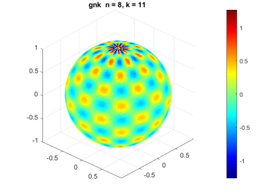
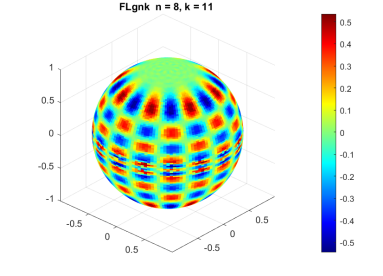
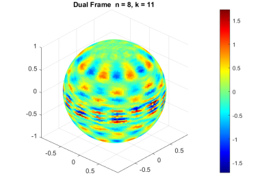
Figure 1: Ingredients of the FD: $b_{nk}$ (left), $e_{nk}$ (middle), $\tilde{e}_{nk}$ (right) for $n=k=8$.

For discretization of the problem, we approximate functions on the sphere with a Chebyshev-type quadrature, i.e., quadrature points such that all weights are equal; see [20]. In our computations, we use quadrature points (spherical design) being exact up to degree 200 taken from [19]. All computations involving spherical harmonics are done using the NFSFT (Non-equispaced fast spherical Fourier transform) software [29, 32]. Note that the dual frame functions of an FD can be pre-computed and stored, such that the computational effort of computing $R^{\ddagger}g$ according to (31) for any new measurement $g$ amounts to one application of the operator $L$ (or $LU_{\alpha}$ in the noisy case), computation of the inner products $\langle Lg,b_{n,k}\rangle_{L_{\text{even}}^{2}(\mathbb{S}^{2})}$ and a summation over these. As starting point for the computation, we only use a finite set of frame functions $\{b_{n,k}:(n,k)\in J,|n|\leq N,k\leq N\}$ for some $N\in\mathbb{N}.$ The frame functions $e_{n,k}=RLb_{n,k}$ are evaluated at the quadrature nodes via the spherical harmonic decomposition (34) up to degree $\ell\leq 100$. The dual frame functions $\tilde{f}_{n,k}$ are computed using the matrix representation of the linear operator $S$ with respect to the basis $b_{n,k}$, see also [27, Chap. 5]. Note that the inversion of this matrix may itself be an ill-conditioned problem requiring regularization. Examples of the involved frame functions are depicted in Figure 1. All computations are performed using Matlab R2022b.

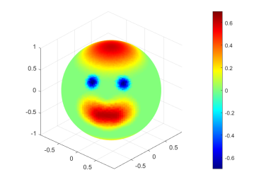
(a)

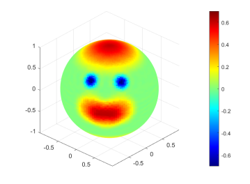
(b)

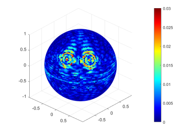
(c)

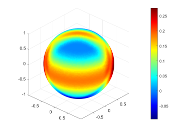
(d)

(e)

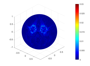
(f)

Figure 2: Reconstruction evaluation for the Chebyshev-type quadrature for different numbers of dual-frame functions used with exact data.

(a)

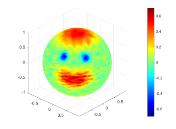
(b)

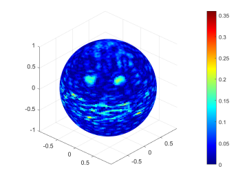
(c)

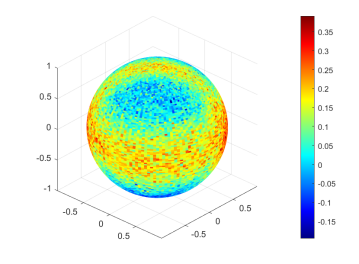
(d)

(e)

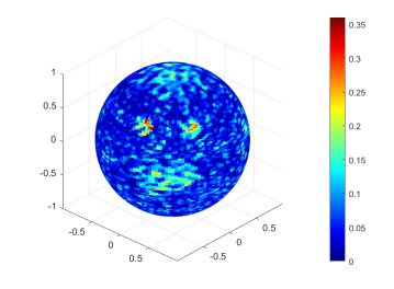
(f)

Figure 3: Reconstruction evaluation for the Chebyshev-type quadrature for different numbers of dual-frame functions used with Gaussian noise $\delta$, noise level $20\%$.

The test function used in our numerical experiments is a linear combination of radially symmetric, quadratic splines, whose Funk-Radon transform is computed explicitly [23, Lem. 4.1], to prevent inverse crimes. Our quality measure is the relative reconstruction error, i.e., $\|f-R^{\ddagger}g\|_{L^{2}(\mathbb{S}^{2})}/\|f\|_{L^{2}(\mathbb{S}^{2})}.$ In Figure 2, we see that increasing the number of used frames highly improves reconstruction quality, reducing the relative reconstruction error from $0.023$ for $N=25$ to $0.006$ for $N=40$. For noisy data shown in Figure 3, the regularization parameter $\alpha$ is chosen such that the relative reconstruction error is minimized. In the case of $N=25$ and noise level $20\%$, the error for the non-regularized solution (i.e., $\alpha=0$) is $0.269,$ while the error for the regularized solution with parameter $\alpha=0.076$ reduces to $0.222.$ However, we see that the increment of the number of frame functions actually results in a loss of reconstruction quality to an error value of $0.332$ (optimally regularized). This can be explained by the regularization effect of the truncation itself: more frame functions result in a less stable reconstruction, but yield a higher accuracy in case of exact data. Note that all specific error values in the noisy case are insignificantly varying for the specific realization of the randomly generated Gaussian noise $\delta$.

5 Conclusion

In this paper, we derived a novel frame decomposition of the Funk-Radon transform utilizing trigonometric basis functions $b_{n,k}$ on the unit sphere and suitable embedding operators in Sobolev spaces. This decomposition does not involve the spherical harmonics and leads to an explicit inversion formula for the Funk-Radon transform. In our numerical examples, we obtained promising reconstruction results even in the case of very large noise by including regularization. While the regularization itself currently uses a spherical harmonics expansion of the operator $L$, in our future work we aim to apply other forms of regularization avoiding the computationally expensive spherical harmonics entirely.

5.0.1 Acknowledgements

This work was funded by the Austrian Science Fund (FWF): project F6805-N36 (SH) and the German Research Foundation (DFG): project 495365311 (MQ) within the SFB F68: “Tomography Across the Scales”. LW is partially supported by the State of Upper Austria.

References

• [1] Abramovich, F., Silverman, B.W.: Wavelet decomposition approaches to statistical inverse problems. Biometrika 85(1), 115–129 (1998)
• [2] Agranovsky, M.L., Rubin, B.: Non-geodesic spherical Funk transforms with one and two centers. In: Bauer, W., Duduchava, R., Grudsky, S., Kaashoek, M. (eds.) Operator Algebras, Toeplitz Operators and Related Topics, pp. 29–52. Birkhäuser, Cham (2020). https://doi.org/10.1007/978-3-030-44651-2_7
• [3] Atkinson, K., Han, W.: Spherical Harmonics and Approximations on the Unit Sphere: An Introduction. Springer, Heidelberg (2012). https://doi.org/10.1007/978-3-642-25983-8
• [4] Bailey, T.N., Eastwood, M.G., Gover, A., Mason, L.: Complex analysis and the Funk transform. J. Korean Math. Soc. 40(4), 577–593 (2003)
• [5] Bellet, J.B.: A discrete Funk transform on the cubed sphere. HAL e-print 03820075 (2022), https://hal.archives-ouvertes.fr/hal-03820075
• [6] Candes, E.J., Donoho, D.L.: Recovering edges in ill-posed inverse problems: optimality of curvelet frames. Ann. Statist. 30(3), 784–842 (2002). https://doi.org/10.1214/aos/1028674842
• [7] Christensen, O.: An Introduction to Frames and Riesz Bases. Applied and Numerical Harmonic Analysis, Birkhäuser, Cham (2016)
• [8] Colonna, F., Easley, G., Guo, K., Labate, D.: Radon transform inversion using the shearlet representation. Appl. Comput. Harmon. Anal. 29(2), 232–250 (2010). https://doi.org/10.1016/j.acha.2009.10.005
• [9] Daubechies, I.: Ten Lectures on Wavelets. Society for Industrial and Applied Mathematics, Philadelphia, PA (1992). https://doi.org/10.1137/1.9781611970104
• [10] Dicken, V., Maass, P.: Wavelet-Galerkin methods for ill-posed problems. J. Inverse Ill-Posed Probl. 4(3), 203–221 (1996). https://doi.org/10.1515/jiip.1996.4.3.203
• [11] Donoho, D.L.: Nonlinear Solution of Linear Inverse Problems by Wavelet–Vaguelette Decomposition. Appl. Comput. Harmon. Anal. 2(2), 101–126 (1995). https://doi.org/10.1006/acha.1995.1008
• [12] Ebner, A., Frikel, J., Lorenz, D., Schwab, J., Haltmeier, M.: Regularization of inverse problems by filtered diagonal frame decomposition. Appl. Comput. Harmon. Anal. 62, 66–83 (2023). https://doi.org/10.1016/j.acha.2022.08.005
• [13] Engl, H.W., Hanke, M., Neubauer, A.: Regularization of inverse problems. Kluwer Academic Publishers, Dordrecht (1996)
• [14] Frikel, J.: Sparse regularization in limited angle tomography. Appl. Comput. Harmon. Anal. 34(1), 117–141 (2013). https://doi.org/10.1016/j.acha.2012.03.005
• [15] Frikel, J., Haltmeier, M.: Efficient regularization with wavelet sparsity constraints in photoacoustic tomography. Inverse Problems 34(2), 024006 (2018). https://doi.org/10.1088/1361-6420/aaa0ac
• [16] Frikel, J., Haltmeier, M.: Sparse regularization of inverse problems by operator-adapted frame thresholding. In: Dörfler, W., Hochbruck, M., Hundertmark, D., Reichel, W., Rieder, A., Schnaubelt, R., Schörkhuber, B. (eds.) Mathematics of Wave Phenomena. pp. 163–178. Springer, Cham (2020)
• [17] Funk, P.: Über Flächen mit lauter geschlossenen geodätischen Linien. Math. Ann. 74(2), 278 – 300 (1913). https://doi.org/10.1007/BF01456044
• [18] Gardner, R.J.: Geometric Tomography. Cambridge University Press, Cambridge, second edn. (2006). https://doi.org/10.1017/CBO9781107341029
• [19] Gräf, M.: Quadrature rules on manifolds. http://www.tu-chemnitz.de/~potts/workgroup/graef/quadrature
• [20] Gräf, M., Potts, D.: On the computation of spherical designs by a new optimization approach based on fast spherical Fourier transforms. Numer. Math. 119, 699–724 (2011). https://doi.org/10.1007/s00211-011-0399-7
• [21] Helgason, S.: Integral Geometry and Radon Transforms. Springer, New York (2011). https://doi.org/10.1007/978-1-4419-6055-9
• [22] Hielscher, R., Potts, D., Quellmalz, M.: An SVD in spherical surface wave tomography. In: Hofmann, B., Leitao, A., Zubelli, J.P. (eds.) New Trends in Parameter Identification for Mathematical Models, pp. 121–144. Birkhäuser, Basel (2018). https://doi.org/10.1007/978-3-319-70824-9_7
• [23] Hielscher, R., Quellmalz, M.: Optimal mollifiers for spherical deconvolution. Inverse Problems 31(8), 085001 (2015). https://doi.org/10.1088/0266-5611/31/8/085001
• [24] Hristova, Y., Moon, S., Steinhauer, D.: A Radon-type transform arising in photoacoustic tomography with circular detectors: spherical geometry. Inverse Probl. Sci. Eng. 24(6), 974–989 (2016). https://doi.org/10.1080/17415977.2015.1088537
• [25] Hubmer, S., Ramlau, R.: A frame decomposition of the atmospheric tomography operator. Inverse Problems 36(9), 094001 (2020). https://doi.org/10.1088/1361-6420/aba4fe
• [26] Hubmer, S., Ramlau, R.: Frame Decompositions of Bounded Linear Operators in Hilbert Spaces with Applications in Tomography. Inverse Problems 37(5), 055001 (2021). https://doi.org/10.1088/1361-6420/abe5b8
• [27] Hubmer, S., Ramlau, R., Weissinger, L.: On regularization via frame decompositions with applications in tomography. Inverse Problems 38(5), 055003 (2022). https://doi.org/10.1088/1361-6420/ac5b86
• [28] Kazantsev, S.G.: Funk–Minkowski transform and spherical convolution of Hilbert type in reconstructing functions on the sphere. Sib. Èlektron. Mat. Izv. 15, 1630–1650 (2018). https://doi.org/10.33048/semi.2018.15.135
• [29] Keiner, J., Kunis, S., Potts, D.: Using NFFT3 - a software library for various nonequispaced fast Fourier transforms. ACM Trans. Math. Software 36, Article 19, 1–30 (2009). https://doi.org/10.1145/1555386.1555388
• [30] Klann, E., Ramlau, R.: Regularization by fractional filter methods and data smoothing. Inverse Problems 24(2) (2008)
• [31] Kudryavtsev, A.A., Shestakov, O.V.: Estimation of the loss function when using wavelet-vaguelette decomposition for solving ill-posed problems. J. Math. Sci. 237, 804–809 (2019). https://doi.org/10.1007/s10958-019-04206-z
• [32] Kunis, S., Potts, D.: Fast spherical Fourier algorithms. J. Comput. Appl. Math. 161, 75–98 (2003). https://doi.org/10.1016/S0377-0427(03)00546-6
• [33] Lee, N.: Wavelet-vaguelette decompositions and homogeneous equations. ProQuest LLC, Ann Arbor, MI (1997), thesis (Ph.D.)–Purdue University
• [34] Louis, A.K., Riplinger, M., Spiess, M., Spodarev, E.: Inversion algorithms for the spherical Radon and cosine transform. Inverse Problems 27(3), 035015 (2011). https://doi.org/10.1088/0266-5611/27/3/035015
• [35] Mildenberger, S., Quellmalz, M.: Approximation properties of the double Fourier sphere method. J. Fourier Anal. Appl. 28 (2022). https://doi.org/10.1007/s00041-022-09928-4
• [36] Minkowski, H.: Sur les corps de largeur constante. Matematiceskij Sbornik 25(3), 505–508 (1905), http://mi.mathnet.ru/sm6643
• [37] Müller, C.: Spherical Harmonics. Springer, Aachen (1966)
• [38] Plonka, G., Potts, D., Steidl, G., Tasche, M.: Numerical Fourier Analysis. Birkhäuser, Cham (2018). https://doi.org/10.1007/978-3-030-04306-3
• [39] Quellmalz, M.: A generalization of the Funk–Radon transform. Inverse Problems 33(3), 035016 (2017). https://doi.org/10.1088/1361-6420/33/3/035016
• [40] Quellmalz, M.: Reconstructing Functions on the Sphere from Circular Means. Dissertation, Universitätsverlag Chemnitz (2019), https://nbn-resolving.org/urn:nbn:de:bsz:ch1-qucosa2-384068
• [41] Quellmalz, M.: The Funk-Radon transform for hyperplane sections through a common point. Anal. Math. Phys. 10(38) (2020). https://doi.org/10.1007/s13324-020-00383-2
• [42] Quellmalz, M., Hielscher, R., Louis, A.K.: The cone-beam transform and spherical convolution operators. Inverse Problems 34(10), 105006 (2018). https://doi.org/10.1088/1361-6420/aad679
• [43] Rauff, A., Timmins, L.H., Whitaker, R.T., Weiss, J.A.: A nonparametric approach for estimating three-dimensional fiber orientation distribution functions (ODFs) in fibrous materials. IEEE Trans. Med. Imaging 41(2), 446–455 (2022). https://doi.org/10.1109/TMI.2021.3115716
• [44] Riplinger, M., Spiess, M.: Numerical inversion of the spherical Radon transform and the cosine transform using the approximate inverse with a special class of locally supported mollifiers. J. Inverse Ill-Posed Probl. 22(4), 497–536 (2013). https://doi.org/10.1515/jip-2012-0095
• [45] Rubin, B.: On the spherical slice transform. Anal. Appl. 20(3), 483–497 (2022). https://doi.org/10.1142/S021953052150024X
• [46] Salman, Y.: Recovering functions defined on the unit sphere by integration on a special family of sub-spheres. Anal. Math. Phys. 7(2), 165–185 (2017). https://doi.org/10.1007/s13324-016-0135-7
• [47] Strichartz, R.S.: $L^{p}$ estimates for Radon transforms in Euclidean and non-Euclidean spaces. Duke Math. J. 48(4), 699–727 (1981)
• [48] Terzioglu, F.: Recovering a function from its integrals over conical surfaces through relations with the Radon transform. Inverse Problems 39(2), 024005 (2023). https://doi.org/10.1088/1361-6420/acad24
• [49] Tuch, D.S.: Q-ball imaging. Magn. Reson. Med. 52(6), 1358–1372 (2004). https://doi.org/10.1002/mrm.20279
• [50] Weissinger, L.: Realization of the Frame Decomposition of the Atmospheric Tomography Operator. Master’s thesis, JKU Linz (2021), https://lisss.jku.at/permalink/f/n2r1to/ULI_alma5185824070003340
• [51] Wilber, H., Townsend, A., Wright, G.B.: Computing with functions in spherical and polar geometries II. the disk. SIAM J. Sci. Comput. 39(3), C238–C262 (2017). https://doi.org/10.1137/16M1070207
• [52] Yarman, C.E., Yazici, B.: Inversion of the circular averages transform using the Funk transform. Inverse Problems 27(6), 065001 (2011). https://doi.org/10.1088/0266-5611/27/6/065001
• [53] Yee, S.Y.K.: Studies on Fourier series on spheres. Mon. Weather Rev. 108(5), 676–678 (1980). https://doi.org/10.1175/1520-0493(1980)108<0676:SOFSOS>2.0.CO;2