Phase transition for detecting a small
community in a large network

Abstract

How to detect a small community in a large network is an interesting problem, including clique detection as a special case, where a naive degree-based $\chi^{2}$-test was shown to be powerful in the presence of an Erdős-Renyi background. Using Sinkhorn’s theorem, we show that the signal captured by the $\chi^{2}$-test may be a modeling artifact, and it may disappear once we replace the Erdős-Renyi model by a broader network model. We show that the recent SgnQ test is more appropriate for such a setting. The test is optimal in detecting communities with sizes comparable to the whole network, but has never been studied for our setting, which is substantially different and more challenging. Using a degree-corrected block model (DCBM), we establish phase transitions of this testing problem concerning the size of the small community and the edge densities in small and large communities. When the size of the small community is larger than $\sqrt{n}$, the SgnQ test is optimal for it attains the computational lower bound (CLB), the information lower bound for methods allowing polynomial computation time. When the size of the small community is smaller than $\sqrt{n}$, we establish the parameter regime where the SgnQ test has full power and make some conjectures of the CLB. We also study the classical information lower bound (LB) and show that there is always a gap between the CLB and LB in our range of interest.

1 Introduction

Consider an undirected network with $n$ nodes and $K$ communities. We assume $n$ is large and the network is connected for convenience. We are interested in testing whether $K=1$ or $K>1$ and the sizes of some of the communities are much smaller than $n$ (communities are scientifically meaningful but mathematically hard to define; intuitively, they are clusters of nodes that have more edges “within” than “across” (Jin, 2015; Zhao et al., 2012)). The problem is a special case of network global testing, a topic that has received a lot of attention (e.g., Jin et al. (2018; 2021b)). However, existing works focused on the so-called balanced case, where the sizes of communities are at the same order. Our case is severely unbalanced, where the sizes of some communities are much smaller than $n$ (e.g., $n^{\varepsilon}$).

The problem also includes clique detection (a problem of primary interest in graph learning (Alon et al., 1998; Ron & Feige, 2010)) as a special case. Along this line, Arias-Castro & Verzelen (2014); Verzelen & Arias-Castro (2015) have made remarkable progress. In detail, they considered the problem of testing whether a graph is generated from a one-parameter Erdős-Renyi model or a two-parameter model: for any nodes $1\leq i,j\leq n$, the probability that they have an edge equals $b$ if $i,j$ both are in a small planted subset and equals $a$ otherwise. A remarkable conclusion of these papers is: a naive degree-based $\chi^{2}$-test is optimal, provided that the clique size is in a certain range. Therefore, at first glance, it seems that the problem has been elegantly solved, at least to some extent.

Unfortunately, recent progress in network testing tells a very different story: the signal captured by the $\chi^{2}$-test may be a modeling artifact. It may disappear once we replace the models in Arias-Castro & Verzelen (2014); Verzelen & Arias-Castro (2015) by a properly broader model. When this happens, the $\chi^{2}$-test will be asymptotically powerless in the whole range of parameter space.

We explain the idea with the popular Degree-Corrected Block Model (DCBM) (Karrer & Newman, 2011), though it is valid in broader settings. Let $A\in\mathbb{R}^{n,n}$ be the network adjacency matrix, where $A(i,j)\in\{0,1\}$ indicates whether there is an edge between nodes $i$ and $j$, $1\leq i,j\leq n$. By convention, we do not allow for self-edges, so the diagonals of $A$ are always 0. Suppose there are $K$ communities, ${\cal C}_{1},\ldots,{\cal C}_{K}$. For each node $i$, $1\leq i\leq n$, we use a parameter $\theta_{i}$ to model the degree heterogeneity and $\pi_{i}$ to model the membership: when $i\in{\cal C}_{k}$, $\pi_{i}(\ell)=1$ if $\ell=k$ and $\pi_{i}(\ell)=0$ otherwise. For a $K\times K$ symmetric and irreducible non-negative matrix $P$ that models the community structure, DCBM assumes that the upper triangle of $A$ contains independent Bernoulli random variables satisfying

$$\mathbb{P}(A(i,j)=1)=\theta_{i}\theta_{j}\pi_{i}^{\prime}P\pi_{j},\qquad 1\leq i,j\leq n.$$ (1.1)

In practice, we interpret $P(k,\ell)$ as the baseline connecting probability between communities $k$ and $\ell$. Write $\theta=(\theta_{1},\theta_{2},\ldots,\theta_{n})^{\prime}$, $\Pi=[\pi_{1},\pi_{2},\ldots,\pi_{n}]^{\prime}$, and $\Theta=\mathrm{diag}(\theta)\equiv\mathrm{diag}(\theta_{1},\theta_{2},\ldots,\theta_{n})$. Introduce $n\times n$ matrices $\Omega$ and $W$ by $\Omega=\Theta\Pi P\Pi^{\prime}\Theta$ and $W=A-\mathbb{E}[A]$. We can re-write (1.1) as

$$A=\Omega-\mathrm{diag}(\Omega)+W.$$ (1.2)

We call $\Omega$ the Bernoulli probability matrix and $W$ the noise matrix. When $\theta_{i}$ in the same community are equal, DCBM reduces to the Stochastic Block Model (SBM) (Holland et al., 1983). When $K=1$, the SBM reduces to the Erdős-Renyi model, where $\Omega(i,j)$ take the same value for all $1\leq i,j\leq n$.

We first describe why the signal captured by the $\chi^{2}$-test in Arias-Castro & Verzelen (2014); Verzelen & Arias-Castro (2015) is a modeling artifact. Using Sinkhorn’s matrix scaling theorem (Sinkhorn, 1974), it is possible to build a null DCBM with $K=1$ that has no community structure and an alternative DCBM with $K\geq 2$ and clear community structure such that the two models have the same expected degrees. Thus, we do not expect that degree-based test such as $\chi^{2}$ can tell them apart. We make this Sinkhorn argument precise in Section 2.1 and show the failure of $\chi^{2}$ in Theorem 2.3.

In the Erdős-Renyi setting in Arias-Castro & Verzelen (2014), the null has one parameter and the alternative has two parameters. In such a setting, we cannot have degree-matching. In these cases, a naive degree-based $\chi^{2}$-test may have good power, but it is due to the very specific models they choose. For clique detection in more realistic settings, we prefer to use a broader model such as the DCBM, where by the degree-matching argument above, the $\chi^{2}$-test is asymptotically powerless.

This motivates us to look for a different test. One candidate is the scan statistic Bogerd et al. (2021). However, a scan statistic is only computationally feasible when each time we scan a very small subset of nodes. For example, if each time we only scan a finite number of nodes, then the computational cost is polynomial; we call the test the Economic Scan Test (EST). Another candidate may come from the Signed-Polygon test family (Jin et al., 2021b), including the Signed-Quadrilateral (SgnQ) as a special case. Let $\hat{\eta}=({\bf 1}_{n}A{\bf 1}_{n})^{-1/2}A{\bf 1}_{n}$ and $\widehat{A}=A-\hat{\eta}\hat{\eta}$. Define $Q_{n}=\sum_{i_{1},i_{2},i_{3},i_{4}(dist)}\widehat{A}_{i_{1}i_{2}}\widehat{A}_{i_{2}i_{3}}\widehat{A}_{i_{3}i_{4}}\widehat{A}_{i_{4}i_{1}}$ where the shorthand $(dist)$ indicates we sum over distinct indices. The SgnQ test statistic is

$$\psi_{n}=\bigl{[}Q_{n}-2(\|\hat{\eta}\|^{2}-1)^{2}\bigr{]}/\sqrt{8(\|\hat{\eta}\|^{2}-1)^{4}}.$$ (1.3)

SgnQ is computationally attractive because it can be evaluated in time $O(n^{2}\bar{d})$, where $\bar{d}$ is the average degree of the network (Jin et al., 2021b).

Moreover, it was shown in Jin et al. (2021b) that (a) when $K=1$ (the null case), $\psi_{n}\rightarrow N(0,1)$, and (b) when $K>1$ and all communities are at the same order (i.e., a balanced alternative case), the SgnQ test achieves the classical information lower bound (LB) for global testing and so is optimal. Unfortunately, our case is much more delicate: the signal of interest is contained in a community with a size that is much smaller than $n$ (e.g., $n^{\varepsilon}$), so the signal can be easily overshadowed by the noise term of $Q_{n}$. Even in the simple alternative case where we only have two communities (with sizes $N$ and $(n-N)$), it is unclear (a) how the lower bounds vary as $N/n\rightarrow 0$, and especially whether there is a gap between the computation lower bound (CLB) and classical information lower bound (LB), and (b) to what extent the SgnQ test attains the CLB and so is optimal.

1.1 Results and contributions

We consider the problem of detecting a small community in the DCBM. In this work, we specifically focus on the case $K=2$ as this problem already displays a rich set of phase transitions, and we believe it captures the essential behavior for constant $K>1$. Let $N\ll n$ denote the size of this small community under the alternative. Our first contribution analyzes the power of SgnQ for this problem, extending results of Jin et al. (2021b) that focus on the balanced case. Let $\lambda_{1}=\lambda_{1}(\Omega)$. In Section 2.2, we define a population counterpart $\tilde{\Omega}$ of $\hat{A}$ and let $\widetilde{\lambda}=\lambda_{1}(\tilde{\Omega})$. We show that SgnQ has full power if $\widetilde{\lambda}_{1}/\sqrt{\lambda_{2}}\to\infty$, which reduces to $N(a-c)/\sqrt{nc}\to\infty$ in the SBM case.

For optimality, we obtain a computational lower bound (CLB), relying on the low-degree polynomial conjecture, which is a standard approach in studying CLB (e.g., Kunisky et al. (2019)). Consider a case where $K=2$ and we have a small community with size $N$. Suppose the edge probability within the community and outside the community are $a$ and $c$, where $a>c$. The quantity $(a-c)/\sqrt{c}$ acts as the Node-wise Signal-to-Noise Ratio (SNR) for the detection problem. When $N\gg\sqrt{n}$, we find that the CLB is completely determined by $N$ and node-wise SNR; moreover, SgnQ matches with the CLB and is optimal. When $N\ll\sqrt{n}$, the situation is more subtle: if the node-wise SNR $(a-c)/\sqrt{c}\rightarrow 0$ (weak signal case), we show the problem is computationally hard and the LB depends on $N$ and the node-wise SNR. If $(a-c)/\sqrt{c}\gg n^{1/2}$ (strong signal case), then SgnQ solves the detection problem. In the range $1\ll(a-c)/\sqrt{c}\ll n^{1/2}$ (moderate signal case), the CLB depends on not only $N$ and the node-wise SNR but also the background edge density $c$. In this regime, we make conjectures of the CLB, from the study of the aforementioned economic scan test (EST). Our results are summarized in Figure 1 and explained in full detail in Section 2.7.

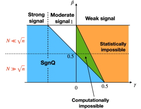
Figure 1: Phase diagram ($(a-c)/\sqrt{c}=n^{-\gamma}$ and $N=n^{1-\beta}$).

We also obtain the classical information lower bound (LB), and discover that as $N/n\rightarrow 0$, there is big gap between CLB and LB. Notably the LB is achieved by an (inefficient) signed scan test. In the balanced case in Jin et al. (2021b), the SgnQ test is optimal among all tests (even those that are allowed unbounded computation time), and such a gap does not exist.

We also show that that the naive degree-based $\chi^{2}$-test is asymptotically powerless due to the aforementioned degree-matching phenomenon.

Our statistical lower bound, computational lower bound, and the powerlessness of $\chi^{2}$ based on degree-matching are also valid for all $K>2$ since any model with $K\geq 2$ contains $K=2$ as a special case. We also expect that our lower bounds are tight for these broader models and that our lower bound constructions for $K=2$ represent the least favorable cases when community sizes are severely unbalanced.

Compared to Verzelen & Arias-Castro (2015); Arias-Castro & Verzelen (2014), we consider network global testing in a more realistic setting, and show that optimal tests there (i.e., a naive degree-based $\chi^{2}$ test) may be asymptotically powerless here. Compared with Bogerd et al. (2021), our setting is very different (they considered a setting where both the null and alternative are DCBM with $K=1$). Compared to the study in the balanced case (e.g., Jin et al. (2018; 2021b); Gao & Lafferty (2017)), our study is more challenging for two reasons. First, in the balanced case, there is no gap between the UB (the upper bound provided by the SgnQ test) and LB, so there is no need to derive the CLB, which is usually technical demanding. Second, the size of the smaller community can get as small as $n^{\varepsilon}$, where $\varepsilon>0$ is any constant. Due this imbalance in community sizes, the techniques of Jin et al. (2021b) do not directly apply. As a result, our proof involves the careful study of the $256$ terms that compose SgnQ, which requires using bounds tailored specifically for the severely unbalanced case.

Our study of the CLB is connected to that of Hajek et al. (2015) in the Erdös-Renyi setting of Arias-Castro & Verzelen (2014). Hajek et al. (2015) proved via computational reducibility that the naive $\chi^{2}$-test is the optimal polynomial-time test (conditionally on the planted clique hypothesis). We also note work of Chen & Xu (2016) that studied a $K$-cluster generalization of the Erdös-Renyi model of Arias-Castro & Verzelen (2014); Verzelen & Arias-Castro (2015) and provided conjectures of the CLB. Compared to our setting, these models are very different because the expected degree profiles of the null and alternative differ significantly. In this work we consider the DCBM model, where due to the subtle phenomenon of degree matching between the null and alternative hypotheses, both CLB and LB are different from those obtained by Hajek et al. (2015).

Notations: We use ${\bf 1}_{n}$ to denote a $n$-dimensional vector of ones. For a vector $\theta=(\theta_{1},\ldots,\theta_{n})$, $\mathrm{diag}(\theta)$ is the diagonal matrix where the $i$-th diagonal entry is $\theta_{i}$. For a matrix $\Omega\in\mathbb{R}^{n\times n}$, $\mathrm{diag}(\Omega)$ is the diagonal matrix where the $i$-th diagonal entry is $\Omega(i,i)$. For a vector $\theta\in\mathbb{R}^{n}$, $\theta_{max}=\max\{\theta_{1},\ldots,\theta_{n}\}$ and $\theta_{min}=\min\{\theta_{1},\ldots,\theta_{n}\}$. For two positive sequences $\{a_{n}\}$ and $\{b_{n}\}$, we write $a_{n}\asymp b_{n}$ if $c_{1}\leq a_{n}/b_{n}\leq c_{2}$ for constants $c_{2}>c_{1}>0$. We say $a_{n}\sim b_{n}$ if $(a_{n}/b_{n})=1+o(1)$.

2 Main results

In Section 2.1, following our discussion on Sinkhorn’s theorem in Section 1, we introduce calibrations (including conditions on identifiability and balance) that are appropriate for severely unbalanced DCBM and illustrate with some examples. In Sections 2.2-2.3, we analyze the power of the SgnQ test and compare it with the $\chi^{2}$-test. In Sections 2.4-2.5, we discuss the information lower bounds (both the LB and CLB) and show that SgnQ test is optimal among polynomial time tests, when $N\gg\sqrt{n}$. In Section 2.6, we study the EST and make some conjectures of the CLB when $N\ll\sqrt{n}$. In Section 2.7, we summarize our results and present the phase transitions.

2.1 DCBM for severely unbalanced networks: identifiability, balance metrics, and global testing

In the DCBM (1.1)-(1.2), $\Omega=\Theta\Pi P\Pi^{\prime}\Theta$. It is known that the matrices $(\Theta,\Pi,P)$ are not identifiable. One issue is that $(\Pi,P)$ are only unique up to a permutation: for a $K\times K$ permutation matrix $Q$, $\Pi P\Pi=(\Pi Q)(Q^{\prime}PQ)(\Pi Q)^{\prime}$. This issue is easily fixable in applications so is usually neglected. A bigger issue is that, $(\Theta,P)$ are not uniquely defined. For example, fixing a positive diagonal matrix $D\in\mathbb{R}^{K\times K}$, let $P^{*}=DPD$ and $\Theta^{*}=\mathrm{diag}(\theta_{1}^{*},\theta_{2}^{*},\ldots,\theta_{n}^{*})$ where $\theta_{i}^{*}=\theta_{i}/\sqrt{D(k,k)}$ if $i\in{\cal C}_{k}$, $1\leq k\leq K$. It is seen that $\Theta\Pi P\Pi^{\prime}\Theta=\Theta^{*}\Pi P^{*}\Pi^{\prime}\Theta^{*}$, so $(\Theta,P)$ are not uniquely defined.

To motivate our identifiability condition, we formalize the degree-matching argument discussed in the introduction. Fix $(\theta,P)$ and let $h=(h_{1},\ldots,h_{K})^{\prime}$ and $h_{k}>0$ is the fraction of nodes in community $k$, $1\leq k\leq K$. By the main result of Sinkhorn (1974), there is a unique positive diagonal matrix $D=\mathrm{diag}(d_{1},\ldots,d_{K})$ such that $DPDh={\bf 1}_{K}$. Consider a pair of two DCBM, a null with $K=1$ and an alternative with $K>1$, with parameters $\Omega=\Theta{\bf 1}_{n}{\bf 1}_{n}^{\prime}\Theta\equiv\theta\theta^{\prime}$ and $\Omega^{*}(i,j)=\theta_{i}^{*}\theta_{j}^{*}\pi_{i}^{\prime}P\pi_{j}$ with $\theta_{i}^{*}=d_{k}\theta_{i}$ if $i\in{\cal C}_{k}$, $1\leq k\leq K$, respectively. Direct calculation shows that node $i$ has the same expected degree under the null and alternative.

There are many ways to resolve the issue. For example, in the balanced case (e.g., Jin et al. (2021b; 2022)), we can resolve it by requiring that $P$ has unit diagonals. However, for our case, this is inappropriate. Recall that, in practice, $P(k,\ell)$ represents as the baseline connecting probability between community $k$ and $\ell$. If we forcefully rescale $P$ to have a unit diagonal here, both $(P,\Theta)$ lose their practical meanings.

Motivated by the degree-matching argument, we propose an identifiability condition that is more appropriate for the severely unbalanced DCBM. By our discussion in Section 1, for any DCBM with a Bernoulli probability matrix $\Omega$, we can always use Sinkhorn’s theorem to define $(\Theta,P)$ (while $\Pi$ is unchanged) such that for the new $(\Theta,P)$, $\Theta=\Theta\Pi P\Pi^{\prime}\Theta$ and $Ph\propto{\bf 1}_{K}$, where $h=(h_{1},\ldots,h_{K})^{\prime}$ and $h_{k}>0$ is the fraction of nodes in community $k$, $1\leq k\leq K$. This motivates the following identifiability condition (which is more appropriate for our case):

$$\|\theta\|_{1}=n,\qquad Ph\propto{\bf 1}_{K},\quad\mbox{where $h_{k}$ is fraction of nodes in ${\cal C}_{k}$, $1\leq k\leq K$}.$$ (2.1)

Lemma 2.1.

For any $\Omega$ that satisfies the DCBM (1.2) and has positive diagonal elements, we can always find $(\Theta,\Pi,P)$ such that $\Omega=\Theta\Pi P\Pi^{\prime}\Theta$ and (2.1) holds. Also, any $(\Theta,P)$ that satisfy $\Omega=\Theta\Pi P\Pi^{\prime}\Theta$ and (2.1) are unique.

Moreover, for network balance, the following two vectors in $\mathbb{R}^{K}$ are natural metrics:

$$d=(\|\theta\|_{1})^{-1}\Pi^{\prime}\Theta{\bf 1}_{n},\qquad g=(\|\theta\|)^{-2}\Pi^{\prime}\Theta^{2}\Pi{\bf 1}_{K},$$ (2.2)

In the balanced case (e.g., Jin et al. (2021b; 2022)), we usually assume the entries of $d$ and $g$ are at the same order. For our setting, this is not the case.

Next we introduce the null and alternative hypotheses that we consider. Under each hypothesis, we impose the identifiability condition (2.1).

General null model for the DCBM. When $K=1$ and $h=1$, $P$ is scalar (say, $P=\alpha$), and $\Omega=\alpha\theta\theta^{\prime}$ satisfies $\|\theta\|_{1}=n$ by (2.1). The expected total degree is $\alpha(\|\theta\|_{1}^{2}-\|\theta\|^{2})\sim\alpha\|\theta\|_{1}^{2}=n^{2}\alpha$ under mild conditions, so we view $\alpha$ as the parameter for network sparsity. In this model, $d=g=1$.

Alternative model for the DCBM . We assume $K=2$ and that the sizes of the two communities, ${\cal C}_{0}$ and ${\cal C}_{1}$, are $(n-N)$ and $N$, respectively. For some positive numbers $a,b,c$, we have

$$P=\left[\begin{array}[]{ll}a&b\\ b&c\\ \end{array}\right],\qquad\mbox{and}\qquad\Omega(i,j)=\left\{\begin{array}[]{ll}\theta_{i}\theta_{j}\cdot a,&\qquad\mbox{if $i,j\in{\cal C}_{1}$},\\ \theta_{i}\theta_{j}\cdot c,&\qquad\mbox{if $i,j\in{\cal C}_{0}$},\\ \theta_{i}\theta_{j}\cdot b,&\qquad\mbox{otherwise}.\\ \end{array}\right.$$ (2.3)

In the classical clique detection problem (e.g., Bogerd et al. (2021)), $a$ and $c$ are the baseline probability where two nodes have an edge when both of them are in the clique and outside the clique, respectively. By (2.1), $a\epsilon+b(1-\epsilon)=b\epsilon+c(1-\epsilon)$ if we write $\epsilon=N/n$. Therefore,

$$b=(c(n-N)-aN)/(n-2N).$$ (2.4)

Note that this is the direct result of Sinkhorn’s theorem and the parameter calibration we choose, not a condition we choose for technical convenience. Write $d=(d_{0},d_{1})^{\prime}$ and $g=(g_{0},g_{1})^{\prime}$. It is seen that $d_{0}=1-d_{1}$, $g_{0}=1-g_{0}$, $d_{1}=\|\theta\|_{1}^{-1}\sum_{i\in{\cal C}_{1}}\theta_{i}$, and $g_{1}=\|\theta\|^{-2}\sum_{i\in{\cal C}_{1}}\theta_{i}^{2}$. If all $\theta_{i}$ are at the same order, then $d_{1}\asymp g_{1}\asymp(N/n)$ and $d_{0}\sim g_{0}\sim 1$. We also observe that $b=c+O(a\epsilon)$ which makes the problem seem very close to Arias-Castro & Verzelen (2014); Bogerd et al. (2021), although in fact the problems are quite different.

Extension . An extension of our alternative is that, for the $K$ communities, the sizes of $m$ of them are at the order of $N$, for an $N\ll n$ and an integer $m$, $1\leq m<K$, and the sizes of remaining $(K-m)$ are at the order of $n$. In this case, $m$ entries of $d$ are $O(N/n)$ and other entries are $O(1)$; same for $g$.

2.2 The SgnQ test: limiting null, p-value, and power

In the null case, $K=1$ and we assume $\Omega=\alpha\theta\theta^{\prime}$, where $\|\theta\|_{1}=n$. As $n\rightarrow\infty$, both $(\alpha,\theta)$ may vary with $n$. Write $\theta_{\max}=\|\theta\|_{\infty}$. We assume

$$n\alpha\to\infty,\qquad\mbox{and}\qquad\alpha\theta^{2}_{\max}\log(n^{2}\alpha)\to 0.$$ (2.5)

The following theorem is adapted from Jin et al. (2021b) and the proof is omitted.

Theorem 2.1 (Limiting null of the SgnQ statistic).

Suppose the null hypothesis is true and the regularity conditions (2.1) and (2.5) hold. As $n\rightarrow\infty$, $\psi_{n}\rightarrow N(0,1)$ in law.

We have two comments. First, since the DCBM has many parameters (even in the null case), it is not an easy task to find a test statistic with a limiting null that is completely parameter free. For example, if we use the largest eigenvalue of $A$ as the test statistic, it is unclear how to normalize it so to have such a limiting null. Second, since the limiting null is completely explicit, we can approximate the (one-sided) $p$-value of $\psi_{n}$ by $\mathbb{P}(N(0,1)\geq\psi_{n})$. The p-values are useful in practice, as we show in our numerical experiments.. For example, using a recent data set on the statisticians’ publication (Ji et al., 2022), for each author, we can construct an ego network and apply the SgnQ test. We can then use the $p$-value to measure the co-authorship diversity of the author. Also, in many hierarchical community detection algorithms (which are presumably recursive, aiming to estimate the tree structure of communities), we can use the p-values to determine whether we should further divide a sub-community in each stage of the algorithm (e.g. Ji et al. (2022)).

The power of the SgnQ test hinges on the matrix $\widetilde{\Omega}=\Omega-({\bf 1}_{n}^{\prime}\Omega{\bf 1}_{n})^{-1}\Omega{\bf 1}_{n}{\bf 1}_{n}^{\prime}\Omega$. By basic algebra,

$$\widetilde{\Omega}=\Theta\Pi\widetilde{P}\Pi^{\prime}\Theta,\qquad\mbox{where \; $\widetilde{P}=P-(d^{\prime}Pd)^{-1}Pdd^{\prime}P$}.$$ (2.6)

Let $\tilde{\lambda}_{1}$ be the largest (in magnitude) eigenvalue of $\widetilde{\Omega}$. Lemma 2.2 is proved in the supplement.

Lemma 2.2.

The rank and trace of the matrix $\widetilde{\Omega}$ are $(K-1)$ and $\|\theta\|^{2}\mathrm{diag}(\tilde{P})^{\prime}g$, respectively. When $K=2$, $\tilde{\lambda}_{1}=\mathrm{trace}(\widetilde{\Omega})=\|\theta\|^{2}(ac-b^{2})(d_{0}^{2}g_{1}+d_{1}^{2}g_{0})/(ad_{1}^{2}+2bd_{0}d_{1}+cd_{0}^{2})$.

As a result of this lemma, we observe that in the SBM case, $d=h$ and thus $\widetilde{\lambda}_{1}=\lambda_{2}\asymp N(a-c)$. To see intuitively that the power of the SgnQ test hinges on $\tilde{\lambda}_{1}^{4}/\lambda_{1}^{2}$, if we heuristically replace the terms of SgnQ by population counterparts, we obtain

$$Q_{n} =\sum_{\begin{subarray}{c}i_{1},i_{2},i_{3},i_{4}(distinct)\end{subarray}}\hat{A}_{i_{1}i_{2}}\hat{A}_{i_{2}i_{3}}\hat{A}_{i_{3}i_{4}}\hat{A}_{i_{4}i_{1}}\approx\mathrm{trace}([\Omega-\eta\eta^{\prime}]^{4})=\mathrm{trace}(\widetilde{\Omega}^{4})=\tilde{\lambda}_{1}^{4}.$$

We now formally discuss the power of the SgnQ test. We focus on the alternative hypothesis in Section 2.1. Let $d=(d_{1},d_{0})^{\prime}$ and $g=(g_{1},g_{0})^{\prime}$ be as in (2.2), and let $\theta_{\max,0}=\max_{i\in{\cal C}_{0}}\theta_{i}$ and $\theta_{\max,1}=\max_{i\in{\cal C}_{1}}\theta_{i}$. Suppose

$$d_{1}\asymp g_{1}\asymp N/n,\qquad a\theta^{2}_{\max,1}=O(1),\qquad cn\to\infty,\qquad c\theta^{2}_{\max,0}\log(n^{2}c)\to 0.$$ (2.7)

These conditions are mild. For example, when $\theta_{i}$’s are at the same order, the first inequality in (2.7) automatically holds, and the other inequalities in (2.7) hold if $a\leq C$ for an absolute constant $C>0$, $cn\to\infty$, and $c\log(n)\to 0$.

Fixing $0<\kappa<1$, let $z_{\kappa}>0$ be the value such that $\mathbb{P}(N(0,1)\geq z_{\kappa})=\kappa$. The level-$\kappa$ SgnQ test rejects the null if and only if $\psi_{n}\geq z_{\kappa}$, where $\psi_{n}$ is as in (1.3). Theorem 2.2 and Corollary 2.1 are proved in the supplement. Recall that our alternative hypothesis is defined in Section 2.1. By power we mean the probability that the alternative hypothesis is rejected, minimized over all possible alternative DCBMs satisfying our regularity conditions.

Theorem 2.2 (Power of the SgnQ test).

Suppose that (2.7) holds, and let $\kappa\in(0,1)$. Under the alternative hypothesis, if $|\tilde{\lambda}_{1}|/\sqrt{\lambda_{1}}\to\infty$, the power of the level-$\kappa$ SgnQ test tends to $1$.

Corollary 2.1.

Suppose the same conditions of Theorem 2.2 hold, and additionally $\theta_{\max}\leq C\theta_{\min}$ so all $\theta_{i}$ are at the same order. In this case, $\lambda_{1}\asymp cn$ and $|\tilde{\lambda}_{1}|\asymp N(a-c)$, and the power of the level-$\kappa$ SgnQ test tends to $1$ if $N(a-c)/\sqrt{cn}\to\infty$.

In Theorem 2.2 and Corollary 2.1, if $\kappa=\kappa_{n}$ and $\kappa_{n}\rightarrow 0$ slowly enough, then the results continues to hold, and the sum of Type I and Type II errors of the SgnQ test at level-$\kappa_{n}$ $\rightarrow 0$.

The power of the SgnQ test was only studied in the balanced case (Jin et al., 2021b), but our setting is a severely unbalanced case, where the community sizes are at different orders as well as the entries of $d$ and $g$. In the balanced case, the signal-to-noise ratio of SgnQ is governed by $|\lambda_{2}|/\sqrt{\lambda}_{1}$, but in our setting, the signal-to-noise ratio is governed by $|\tilde{\lambda}_{1}|/\sqrt{\lambda_{1}}$. The proof is also subtly different. Since the entries of $P$ are at different orders, many terms deemed negligible in the power analysis of the balanced case may become non-negligible in the unbalanced case and require careful analysis.

2.3 Comparison with the naive degree-based $\chi^{2}$-test

Consider a setting where $\Omega=\alpha\Theta{\bf 1}_{n}{\bf 1}_{n}^{\prime}\Theta\equiv\alpha\theta\theta^{\prime}$ under the null and $\Omega=\Theta\Pi P\Pi^{\prime}\Theta$ under the alternative, and (2.1) holds. When $\theta$ is unknown, it is unclear how to apply the $\chi^{2}$-test: the null case has $n$ unknown parameters $\theta_{1},\ldots,\theta_{n}$, and we need to use the degrees to estimate $\theta_{i}$ first. As a result, the resultant $\chi^{2}$-statistic may be trivially $0$. Therefore, we consider a simpler SBM case where $\theta={\bf 1}_{n}$. In this case, $\Omega=\alpha{\bf 1}_{n}{\bf 1}_{n}$, and $\Omega=\Pi P\Pi^{\prime}$ and the null case only has one unknown parameter $\alpha$. Let $y_{i}$ be the degree of node $i$, and let $\hat{\alpha}=[n(n-1)]^{-1}{\bf 1}_{n}^{\prime}A{\bf 1}_{n}$. The $\chi^{2}$-statistic is

$$X_{n}=\sum_{i=1}^{n}(y_{i}-n\hat{\alpha})^{2}/[(n-1)\hat{\alpha}(1-\hat{\alpha})].$$ (2.8)

It is seen that as $n\alpha\to\infty$ and $\alpha\to 0$, $(X_{n}-n)/\sqrt{2n}\rightarrow N(0,1)$ in law. For a fixed level $\kappa\in(0,1)$, consider the $\chi^{2}$-test that rejects the null if and only if $(X_{n}-n)/\sqrt{2n}>z_{\kappa}$. Let $\alpha_{0}=n^{-2}({\bf 1}_{n}^{\prime}\Omega{\bf 1}_{n})$. The power of the $\chi^{2}$-test hinges on the quantity $(n\alpha_{0})^{-1}\|(\Omega{\bf 1}_{n}-n\alpha_{0})\|^{2}=(n\alpha_{0})^{-1}\|\Pi Ph-(h^{\prime}Ph)^{-1}{\bf 1}_{n}\|^{2}=0$, if $Ph\propto{\bf 1}_{K}$. The next theorem is proved in the supplement.

Theorem 2.3.

Suppose $\theta=\mathbf{1}_{n}$ and (2.7) holds. If $|\tilde{\lambda}_{1}|/\sqrt{\lambda_{1}}\to\infty$ under the alternative hypothesis, the power of the level-$\kappa$ SgnQ test goes to $1$, while the power of the level-$\kappa$ $\chi^{2}$-test goes to $\kappa$.

2.4 The statistical lower bound and the optimality of the scan test

For lower bounds, it is standard to consider a random-membership DCBM (Jin et al., 2021b), where $\|\theta\|_{1}=n$, $P$ is as in (2.3)-(2.4) and for a number $N\ll n$, $\Pi=[\pi_{1},\pi_{2},\ldots,\pi_{n}]^{\prime}$ satisfies

$$\pi_{i}=(X_{i},1-X_{i}),\qquad\mbox{where $X_{i}$ are iid Bernoulli($\varepsilon)$ with $\varepsilon=N/n$}.$$ (2.9)

Theorem 2.4 (Statistical lower bound).

Consider the null and alternative hypotheses of Section 2.1, and assume that (2.9) is satisfied, $\theta_{\max}\leq C\theta_{\min}$ and $Nc/\log n\to\infty$. If $\sqrt{N}(a-c)/\sqrt{c}\to 0$, then for any test, the sum of the type-I and type-II errors tends to $1$.

To show the tightness of this lower bound, we introduce the signed scan test, by adapting the idea in Arias-Castro & Verzelen (2014) from the SBM case to the DCBM case. Unlike the SgnQ test and the $\chi^{2}$-test, signed scan test is not a polynomial time test, but it provides sharper upper bounds. Let $\hat{\eta}$ be the same as in (1.3). For any subset $S\subset\{1,2,\ldots,n\}$, let ${\bf 1}_{S}\in\mathbb{R}^{n}$ be the vector whose $i$th coordinate is $1\{i\in S\}$. Define the signed scan statistic

$$\phi_{sc}=\max_{S\subset\{1,2,\ldots,n\}:|S|=N}{\bf 1}^{\prime}_{S}\big{(}A-\hat{\eta}\hat{\eta}^{\prime}\big{)}{\bf 1}_{S}.$$ (2.10)

Theorem 2.5 (Tightness of the statistical lower bound).

Consider the signed scan test (2.10) that rejects the null hypothesis if $\phi_{sc}>t_{n}$. Under the assumptions of Theorem 2.4, if $\sqrt{N}(a-c)/\sqrt{c\log(n)}\to\infty$, then there exists a sequence $t_{n}$ such that the sum of type I and type II errors of the signed scan test tends to $0$.

By Theorems 2.4-2.5 and Corollary 2.1, the two hypotheses are asymptotically indistinguishable if $\sqrt{N}(a-c)/\sqrt{c}\to 0$, and are asymptotically distinguishable by the SgnQ test if $N(a-c)/\sqrt{cn}\to\infty$. Therefore, the lower bound is sharp, up to log-factors, and the signed scan test is nearly optimal. Unfortunately, the signed scan test is not polynomial-time computable. Does there exist a polynomial-time computable test that is optimal? We address this in the next section.

2.5 The computational lower bound

Consider the same hypothesis pair as in Section 2.4, where $K=2$, $P$ is as in (2.3)-(2.4), and $\Pi$ is as in (2.9). For simplicity, we only consider SBM, i.e., $\theta_{i}\equiv 1$. The low-degree polynomials argument emerges recently as a major tool to predicting the average-case computational barriers in a wide range of high-dimensional problems (Hopkins & Steurer, 2017; Hopkins et al., 2017). Many powerful methods, such as spectral algorithms and approximate message passing, can be formulated as functions of the input data, where the functions are polynomials with degree at most logarithm of the problem dimension. In comparison to many other schemes of developing computational lower barriers, the low-degree polynomial method yields the same threshold for various average-case hardness problems, such as community detection in the SBM (Hopkins & Steurer, 2017) and (hyper)-planted clique detection (Hopkins, 2018; Luo & Zhang, 2022). The foundation of the low-degree polynomial argument is the following low-degree polynomial conjecture (Hopkins et al., 2017) :

Conjecture 2.1 (Adapted from Kunisky et al. (2019)).

Let $\mathbb{P}_{n}$ and $\mathbb{Q}_{n}$ denote a sequence of probability measures with sample space $\mathbb{R}^{n^{k}}$ where $k=O(1)$. Suppose that every polynomial $f$ of degree $O(\log n)$ with $\mathbb{E}_{\mathbb{Q}_{n}}f^{2}=1$ is bounded under $\mathbb{P}_{n}$ with high probability as $n\to\infty$ and that some further regularity conditions hold. Then there is no polynomial-time test distinguishing $\mathbb{P}_{n}$ from $\mathbb{Q}_{n}$ with type I and type II error tending to $0$ as $n\to\infty$.

We refer to Hopkins (2018) for a precise statement of this conjecture’s required regularity conditions. The low-degree polynomial computational lower bound for our testing problem is as follows.

Theorem 2.6 (Computational lower bound).

Consider the null and alternative hypotheses in Section 2.1, and assume $\theta_{i}\equiv 1$ and (2.9) holds. As $n\to\infty$, assume $c<a$, $c<1-\delta$ for constant $\delta>0$, $N<n/3$, $D=O(\log n)$, and $\limsup_{n\to\infty}\left\{\left(\log_{n}\frac{N}{\sqrt{n}}+\log_{n}\frac{a-c}{\sqrt{c}}\right)\vee\left(\sqrt{D/2-1}\log_{n}\frac{a-c}{\sqrt{c}}\right)\right\}<0.$ For any series of degree-$D$ polynomials $\phi_{n}:A\to\mathbb{R}$, whenever $\mathbb{E}_{H_{0}}\phi_{n}(A)=0,\textrm{Var}_{H_{0}}(\phi_{n}(A))=1$, we must have $\mathbb{E}_{H_{1}}\phi_{n}(A)=o(1)$. This implies if Conjecture 2.1 is true, there is no consistent polynomial-time test for this problem.

By Theorem 2.6, if both $(a-c)/\sqrt{c}\lesssim 1$ and $N(a-c)/\sqrt{cn}\to 0$, the testing problem is computationally infeasible. The region where the testing problem is statistically possible but the SgnQ test loses power corresponds to $N(a-c)/\sqrt{cn}\to 0$. If $N\gtrsim\sqrt{n}$, Theorem 2.6 already implies that this is the computationally infeasible region; in other words, SgnQ achieves the CLB and is optimal. If $N=o(\sqrt{n})$, SgnQ solves the detection problem only when $(a-c)/\sqrt{c}\gg n^{1/2}$, i.e. when the node-wise SNR is strong. We discuss the case of moderate node-wise SNR in the next subsection.

2.6 The power of EST, and discussions of the tightness of CLB

When $N=o(\sqrt{n})$ and $(a-c)/\sqrt{c}\to\infty$ both hold, the upper bound by SgnQ does not match with the CLB. It is unclear whether the CLB is tight. To investigate the CLB in this regime, we consider other possible polynomial-time tests. The economic scan test (EST) is one candidate. Given fixed positive integers $v$ and $e$, the EST statistic is defined to be $\phi_{EST}^{(v)}\equiv\sup_{|S|\leq v}\sum_{i,j\in S}A_{ij}$, and the EST is defined to reject if and only if $\phi_{EST}^{(v)}\geq e$. EST can be computed in time $O(n^{v})$, which is polynomial time. For simplicity, we consider the SBM, i.e. where $\theta={\bf 1}_{n}$, and a specific setting of parameters for the null and alternative hypotheses.

Theorem 2.7 (Power of EST).

Suppose $\beta\in[1/2,1)$ and $0<\omega<\delta<1$ are fixed constants. Under the alternative, suppose $\theta=\mathbf{1}_{n}$, (2.9) holds, $N=n^{1-\beta}$, $a=n^{-\omega}$, and $c=n^{-\delta}$. Under the null, suppose $\theta=\mathbf{1}_{n}$ and $\alpha=a(N/n)+b(1-N/n)$. If $\omega/(1-\beta)<\delta$, the sum of type I and type II errors of the EST with $v$ and $e$ satisfying $\omega/(1-\beta)<v/e<\delta$ tends to $0$.

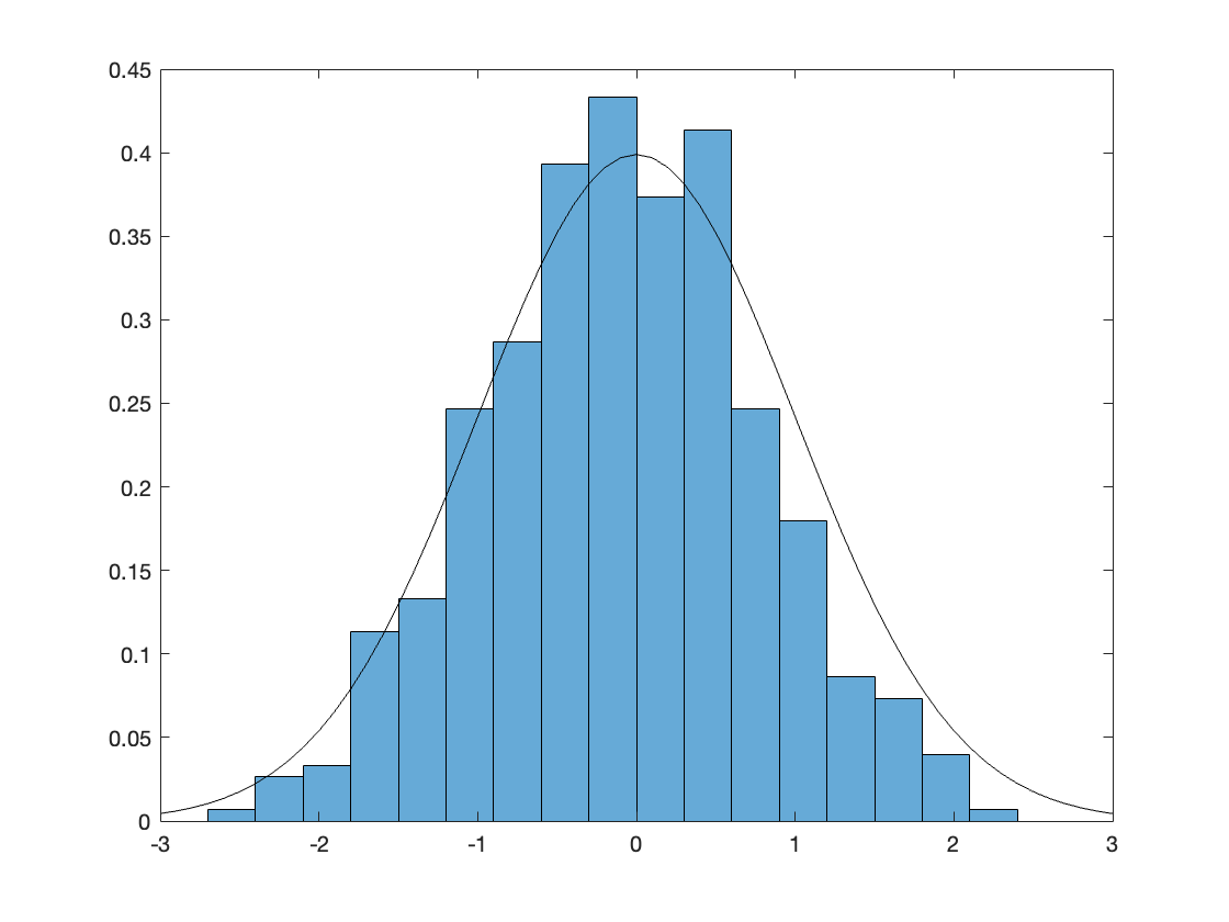
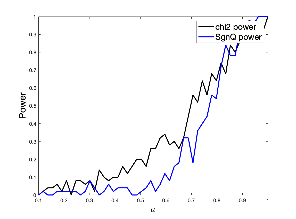
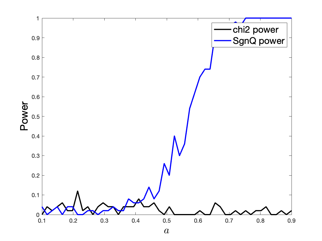
Figure 2: Left: Null distribution of SgnQ ($n=500$). Middle and right: Power comparison of SgnQ and $\chi^{2}$ ($n=100$, $N=10$, 50 repetitions). We consider a 2-community SBM with $P_{11}=a$, $P_{22}=0.1$, $P_{12}=0.1$ (middle plot) and $P_{12}=\frac{an-(a+0.1)N}{n}$ (right plot, the case of degree matching).

Theorem 2.7 follows from standard results in probabilistic combinatorics (Alon & Spencer, 2016). It is conjectured in Bhaskara et al. (2010) that EST attains the CLB in the Erdös-Renyi setting considered by Arias-Castro & Verzelen (2014); Verzelen & Arias-Castro (2015). This suggests that the CLB in Theorem 2.6 is likely not tight when $N=o(\sqrt{n})$ and $(a-c)/\sqrt{c}\to\infty$. However, this is not because our inequalities in proving the CLB are loose. A possible reason is that the prediction from the low-degree polynomial conjecture does not provide a tight bound. It remains an open question whether other computational infeasibility frameworks provide a tight CLB in our problem.

2.7 The phase transition

We describe more precisely our results in terms of the phase transitions shown in Figure 1. Consider the null and alternative hypotheses from Section 2.1. For illustration purposes, we fix constants $\beta\in(0,1)$ and $\gamma\in\mathbb{R}$ and assume that $N=n^{1-\beta}$ and $(a-c)/\sqrt{c}=n^{-\gamma}$. In the two-dimensional space of $(\gamma,\beta)$, the region of $\beta>1/2$ and $\beta<1/2$ corresponds to that the size of the small community is $\gg\sqrt{n}$ and $o(\sqrt{n})$, respectively, and the regions of $\gamma>0$, $-1/2<\gamma<0$ and $\gamma<-1/2$ correspond to ‘weak node-wise signal’, ‘moderate node-wise signal,’ and the ‘strong node-wise signal’, respectively. See Figure 1. By our results in Section 2.4, the testing problem is statistically impossible if $\beta+2\gamma>1$ (orange region). By our results in Section 2.2, SgnQ has a full power if $\beta+\gamma<1/2$ (blue region). Our results in Section 2.5 state that the testing problem is computationally infeasible if both $\gamma>0$ and $\beta+\gamma>1/2$ (green and orange regions). Combining these results, when $\beta<1/2$, we have a complete understanding of the LB and CLB.

3 Numerical results

Simulations. First in Figure 2 (left panel) we demonstrate the asymptotic normality of SgnQ under a null of the form $\Omega=\theta\theta^{\prime}$, where $\theta_{i}$ are i.i.d. generated from $\mathrm{Pareto}(4,0.375)$. Though the degree heterogeneity is severe, SgnQ properly standardized is approximately standard normal under the null. Next in Figure 2 we compare the power of SgnQ in an asymmetric and symmetric SBM model. As our theory predicts, both tests are powerful when degrees are not calibrated in each model, but only SgnQ is powerful in the symmetric case. We also compare the power of SgnQ with the scan test to show evidence of a statistical-computational gap. We relegate these experiments to the supplement.

Real data: Next we demonstrate the effectiveness of SgnQ in detecting small communities in coauthorship networks studied in Ji et al. (2022). In Example 1, we consider the personalized network of Raymond Carroll, whose nodes consist of his coauthors for papers in a set of 36 statistics journals from the time period 1975 – 2015. An edge is placed between two coauthors if they wrote a paper in this set of journals during the specified time period. The SgnQ p-value for Carroll’s personalized network $G_{\mathsf{Carroll}}$ is $0.02$, which suggests the presence of more than one community. In Ji et al. (2022), the authors identify a small cluster of coauthors from a collaboration with the National Cancer Institute. We applied the SCORE community detection module with $K=2$ (e.g. Ke & Jin (2022)) and obtained a larger community $G_{\mathsf{Carroll}}^{\,0}$ of size $218$ and a smaller community $G_{\mathsf{Carroll}}^{\,1}$ of size $17$. Precisely, we removed Carroll from his network, applied SCORE on the remaining giant component, and defined $G_{\mathsf{Carroll}}^{\,0}$ to be the complement of the smaller community. The SgnQ p-values in the table below suggest that both $G_{\mathsf{Carroll}}^{\,0}$ and $G_{\mathsf{Carroll}}^{\,1}$ are tightly clustered. Refer to the supplement for a visualization of Carroll’s network and its smaller community labeled by author names. In Example 2, we consider three different coauthorship networks $G_{\mathsf{old}}$, $G_{\mathsf{recent}}$, and $G_{\mathsf{new}}$ corresponding to time periods (i) 1975-1997, (ii) 1995-2007, and (iii) 2005-2015 for the journals AoS, Bka, JASA, and JRSSB. Nodes are given by authors, and an edge is placed between two authors if they coauthored at least one paper in one of these journals during the corresponding time period. For each network, we perform a similar procedure as in the first example. First we compute the SgnQ p-value, which turns out to be $\approx 0$ (up to 16 digits of precision) for all networks. For each $i\in\{\mathsf{old},\mathsf{recent},\mathsf{new}\}$, we apply SCORE with $K=2$ to $G_{i}$ and compute the SgnQ p-value on both resulting communities, let us call them $G_{i}^{0}$ and $G_{i}^{1}$. We refer to the table below for the results. For $G_{\mathsf{old}}$ and $G_{\mathsf{recent}}$, SCORE with $K=2$ extracts a small community. The SgnQ p-value further supports the hypothesis that this small community is well-connected. In the last network, SCORE splits $G_{\mathsf{new}}$ into two similarly sized pieces whose p-values suggests they can be split into smaller subcommunities.

Example	Network	Size	SgnQ p-value	Communities	Sizes	SgnQ p-values
1	$G_{\mathsf{Carroll}}$	235	0.02	$(G_{\mathsf{Carroll}}^{\,0},G_{\mathsf{Carroll}}^{1})$	(218, 17)	(0.134, 0.682)
2	$G_{\mathsf{old}}$	2647	0	$(G_{\mathsf{old}}^{0},G_{\mathsf{old}}^{1})$	(2586, 61)	(0, 0.700)
	$G_{\mathsf{recent}}$	2554	0	$(G_{\mathsf{recent}}^{0},G_{\mathsf{recent}}^{1})$	(2540,14)	(0, 0.759)
	$G_{\mathsf{new}}$	2920	0	$(G_{\mathsf{new}}^{0},G_{\mathsf{new}}^{1})$	(1685,1235)	(0, 0)

Discussions: Global testing is a fundamental problem and often the starting point of a long line of research. For example, in the literature of Gaussian models, certain methods started as a global testing tool, but later grew into tools for variable selection, classification, and clustering and motivated many researches (e.g., Donoho & Jin (2004; 2015)). The SgnQ test may also motivate tools for many other problems, such as estimating the locations of the clique and clustering more generally. For example, in Jin et al. (2022), the SgnQ test motivated a tool for estimating the number of communities (see also Ma et al. (2021)). SgnQ is also extendable to clique detection in a tensor (Yuan et al., 2021; Jin et al., 2021a) and for network change point detection. The LB and CLB we obtain in this paper are also useful for studying other problems, such as clique estimation. If you cannot tell whether there is a clique in the network, then it is impossible to estimate the clique. Therefore, the LB and CLB are also valid for the clique estimation problem (Alon et al., 1998; Ron & Feige, 2010).

The limiting distribution of SgnQ is $N(0,1)$. This is not easy to achieve if we use other testing ideas, such as the leading eigenvalues of the adjacency matrix: the limiting distribution depends on many unknown parameters and it is hard to normalize (Liu et al., 2019). The p-value of the SgnQ test is easy to approximate and also useful in applications. For example, we can use it to measure the research diversity of a given author. Consider the ego sub-network of an author in a large co-authorship or citation network. A smaller p-value suggests that the ego network has more than $1$ communitiy and has more diverse interests. The p-values can also be useful as a stopping criterion in hierarchical community detection modules.

Acknowledgments. We thank the anonymous referees for their helpful comments. We thank Louis Cammarata for assistance with the simulations in Section A.3. J. Jin was partially supported by NSF grant DMS-2015469. Z.T. Ke was supported in part by NSF CAREER Grant DMS-1943902. A.R. Zhang acknowledges the grant NSF CAREER-2203741.

Appendix

Appendix A Additional experiments

A.1 Visualization of Carroll’s network

In Figure 3, we display a subgraph of high-degree nodes of Raymond Carroll’s personalized coauthorship network (figure borrowed with permission from Ji et al. (2022)). On the right of Figure 3 is shown the small community extracted by SCORE, and this cluster of size $17$ is labeled by author names.

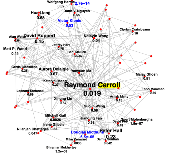
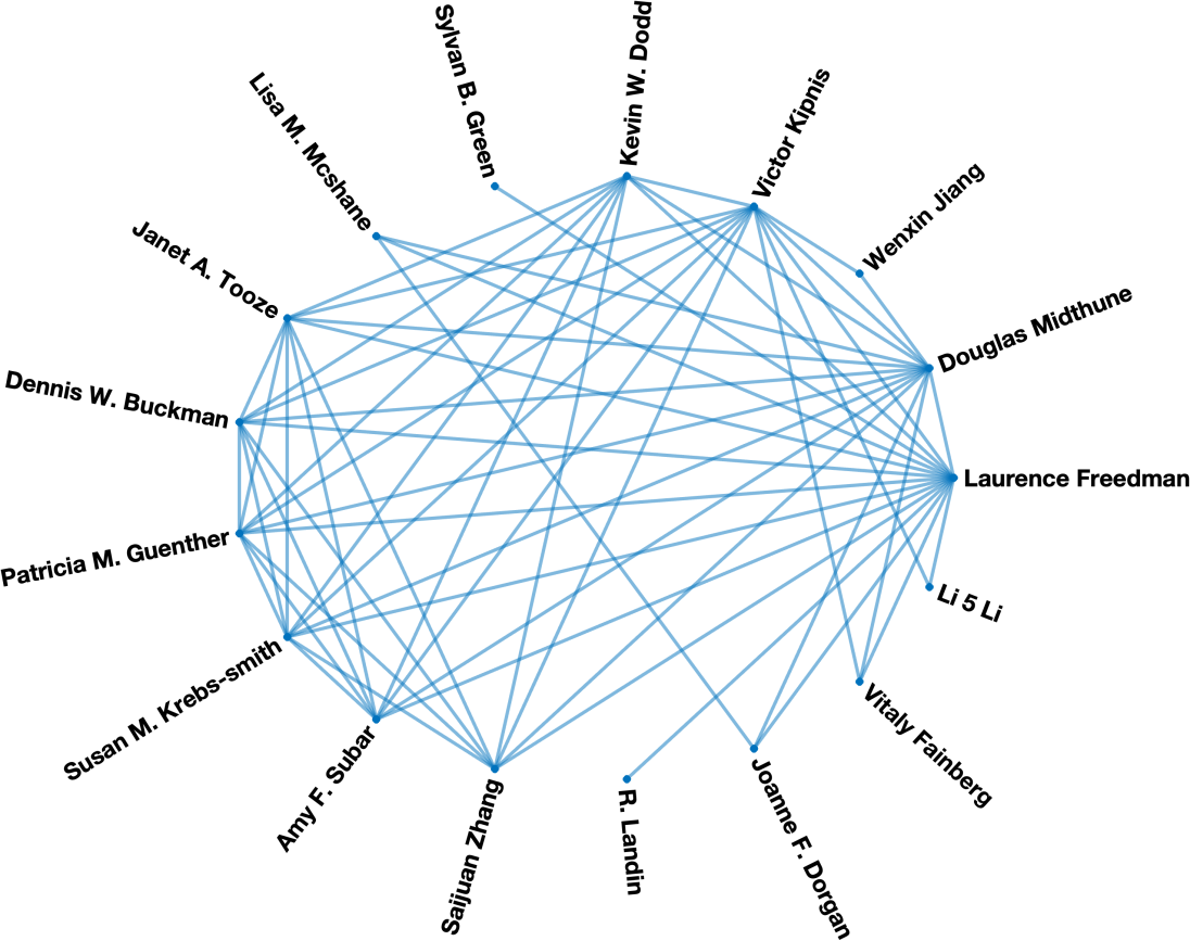
Figure 3: Left: Carroll’s personalized network, figure taken from Ji et al. (2022). Right: A small community of $17$ authors extracted by SCORE and whose SgnQ p-value is $0.6818$.

A.2 SgnQ vs. Scan

In this section we demonstrate evidence of a statistical-computational gap by means of numerical experiments.

We consider a SBM null and alternative model (as in Example 2 with $\theta\equiv 1$) with

$$P_{0}=\begin{pmatrix}\alpha&\alpha\\ \alpha&\alpha\end{pmatrix},\qquad P_{1}=\begin{pmatrix}a&b\\ b&c\end{pmatrix}$$

where $aN+b(n-N)=\alpha$. For this simple testing problem, we compare the power of SgnQ and the scan test. In our experiments, we set $\alpha=0.2$ and allow the parameter $a$ to vary from $a=\alpha$ to $a=a_{\max}\equiv an/N$. Once $a$ and $\alpha$ are fixed, the parameters $b$ and $c$ are determined by

$$c =\frac{aN^{2}+\alpha n^{2}-2\alpha nN}{(n-N)^{2}},$$

$$b =\frac{nc-(a+c)N}{n-2N}.$$

In particular, $a_{\max}$ is the largest value of $a$ such that $b\geq 0$.

Since the scan test $\phi_{sc}$ we defined is extremely computationally expensive, we study the power of an ‘oracle’ scan test $\tilde{\phi}_{sc}$ which knows the location of the true planted subset $\mathcal{C}_{1}$. The power of the oracle scan test is computed as follows. Let $\kappa$ denote the desired level.

1. Using $M_{cal}$ repetitions under the null, we calculate the (non-oracle) scan statistic $\phi_{sc}^{(1)},\ldots,\phi_{sc}^{(M_{cal})}$ for each repetition. We set the threshold $\hat{\tau}$ to be the empirical $1-\kappa$ quantile of $\phi_{sc}^{(1)},\ldots,\phi_{sc}^{(M_{cal})}$.

2. Given a sample from the alternative model, we compute the power using $M_{pow}$ repetitions, where we reject if

   $$\tilde{\phi}_{sc}\equiv\mathbf{1}_{\mathcal{C}_{1}}(A-\hat{\eta}\hat{\eta}^{\prime})\mathbf{1}_{\mathcal{C}_{1}}>\hat{\tau}.$$

In our experiments, we set $M_{cal}=75$ and $M_{pow}=200$.

Note that since $\tilde{\phi}_{sc}\leq\phi_{sc}$, the procedure above gives an underestimate of the power of the scan test (provide the threshold is correctly calibrated), which is helpful since this can be used to show evidence of a statistical-computational gap.

In our plots we also indicate the statistical (information-theoretic) and computational thresholds in addition to the power. Inspired by the sharp characterization of the statistical threshold in (Arias-Castro & Verzelen, 2014, Equation (10)) for planted dense subgraph, in all plots we draw a black vertical dashed line at the first value of $a$ such that

$$(1/2)\sqrt{N}(a-c)/\sqrt{c(1-c)}>1.$$

We draw a blue vertical dashed line at the first value of $a$ such that

$$N(a-c)/\sqrt{nc}>1.$$

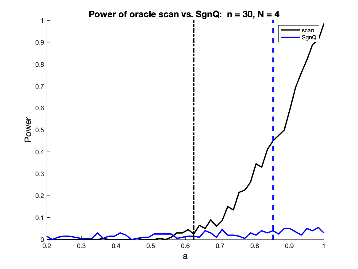
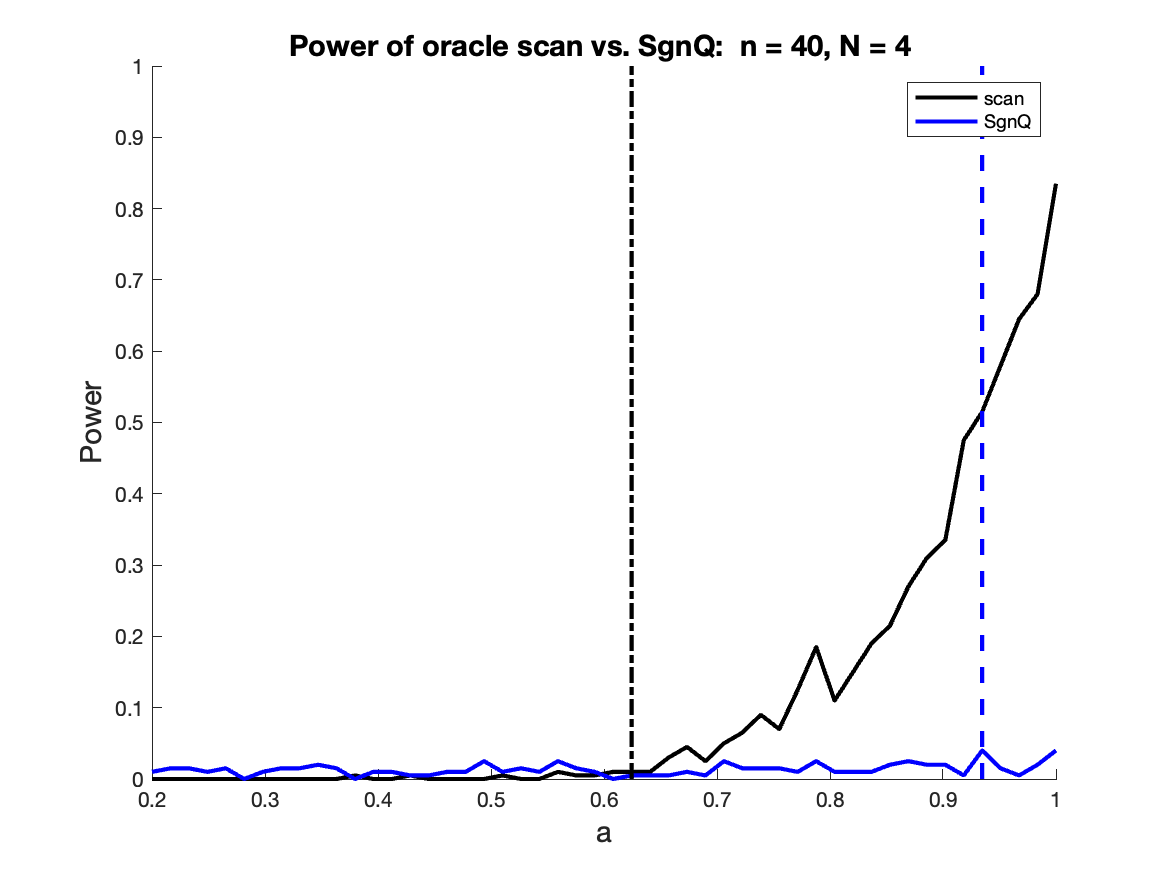
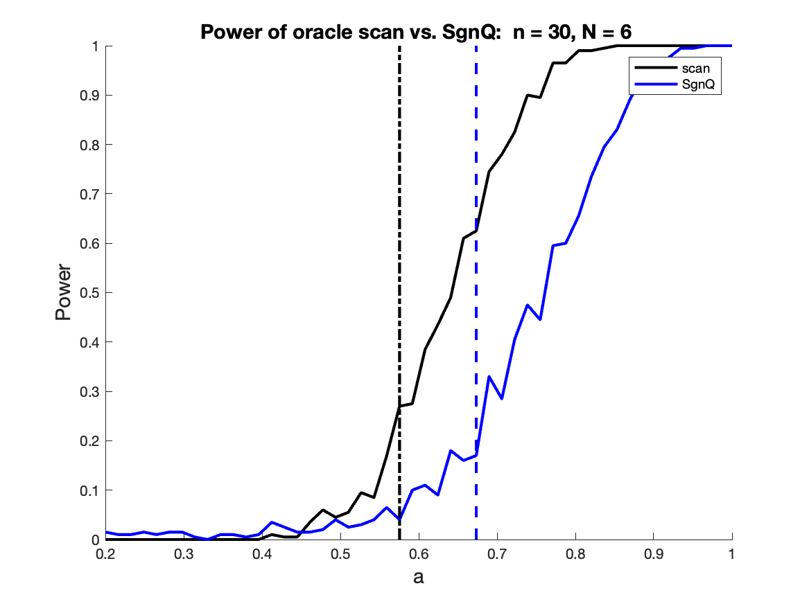
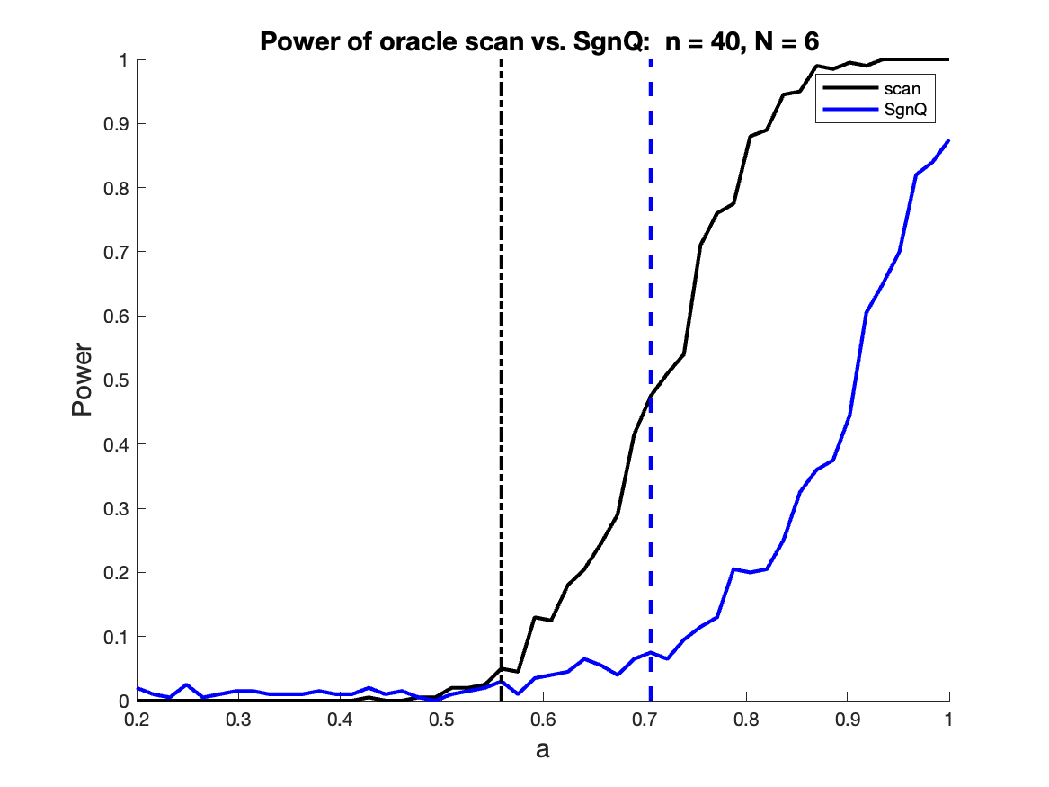
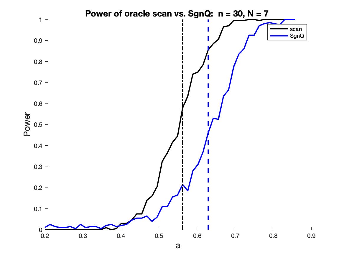
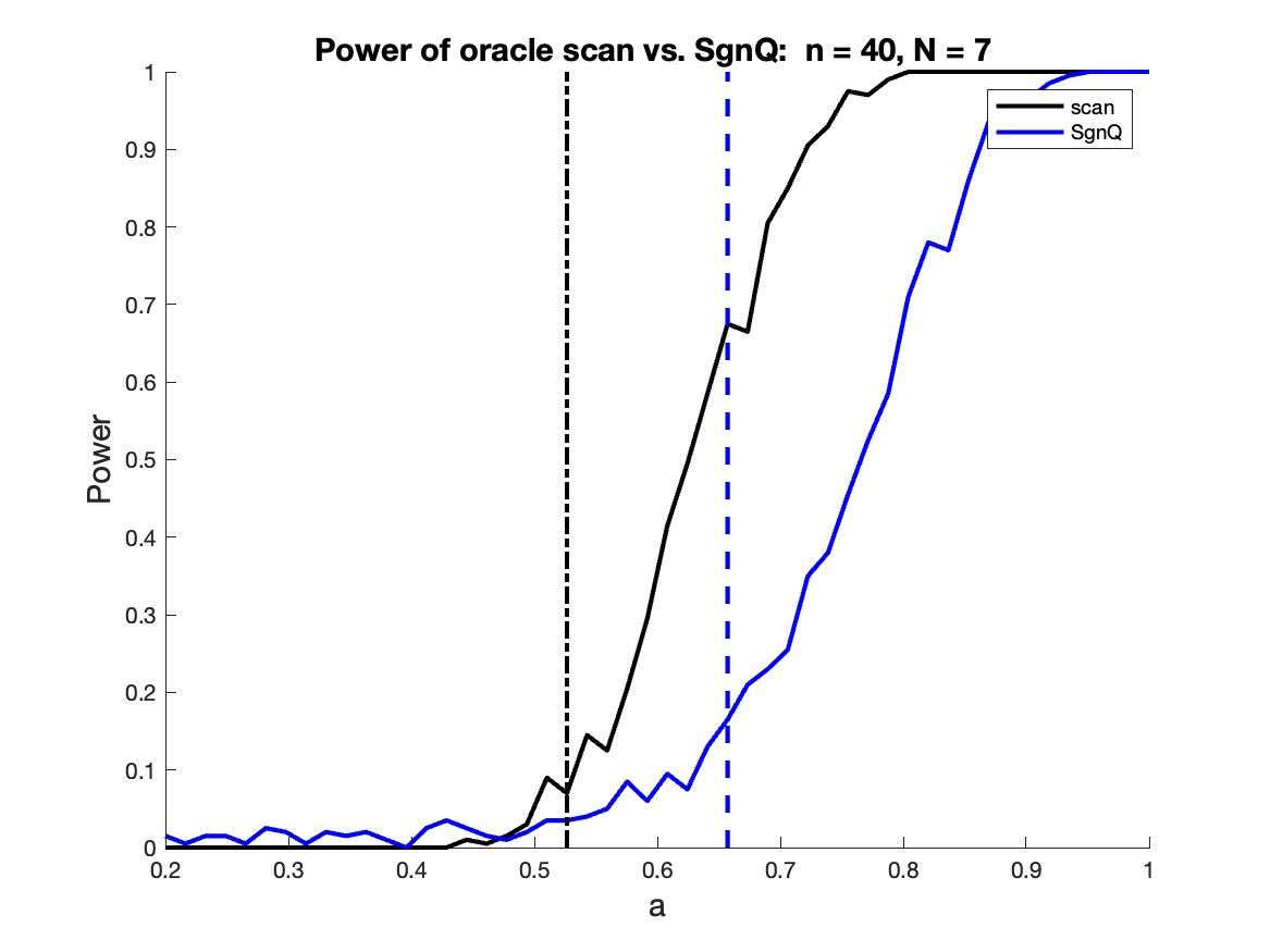
Figure 4: The power of SgnQ (blue curve) and oracle scan (black curve) for $n=30,N\in\{4,6,7\}$ (left) and $n=40,N\in\{4,6,7\}$ (right). The black dashed line indicates the theoretical statistical threshold, and the blue dashed line indicates the theoretical computational threshold.

A.3 $\chi_{2}$ vs. SgnQ

We also show additional experiments demonstrating the effect of degree-matching on the power of the $\chi^{2}$ test. We compute the power with respect to the following alternative models (as in Example 2 with $\theta\equiv 1$) with

$$P^{(1)}=\begin{pmatrix}a&b\\ b&c\end{pmatrix},\qquad P^{(2)}=\begin{pmatrix}a&c\\ c&c\end{pmatrix}$$

where $b=\frac{cn-(a+c)N}{n-2N}$, $c$ is fixed, and $a$ ranges from $c$ to $a_{\max}^{\prime}=c(n-N)/N$ for the experiments with $P^{(1)}$. Similar to before, $a_{\max}^{\prime}$ is the largest value of $a$ such that $b\geq 0$. See Figure 5 for further details.

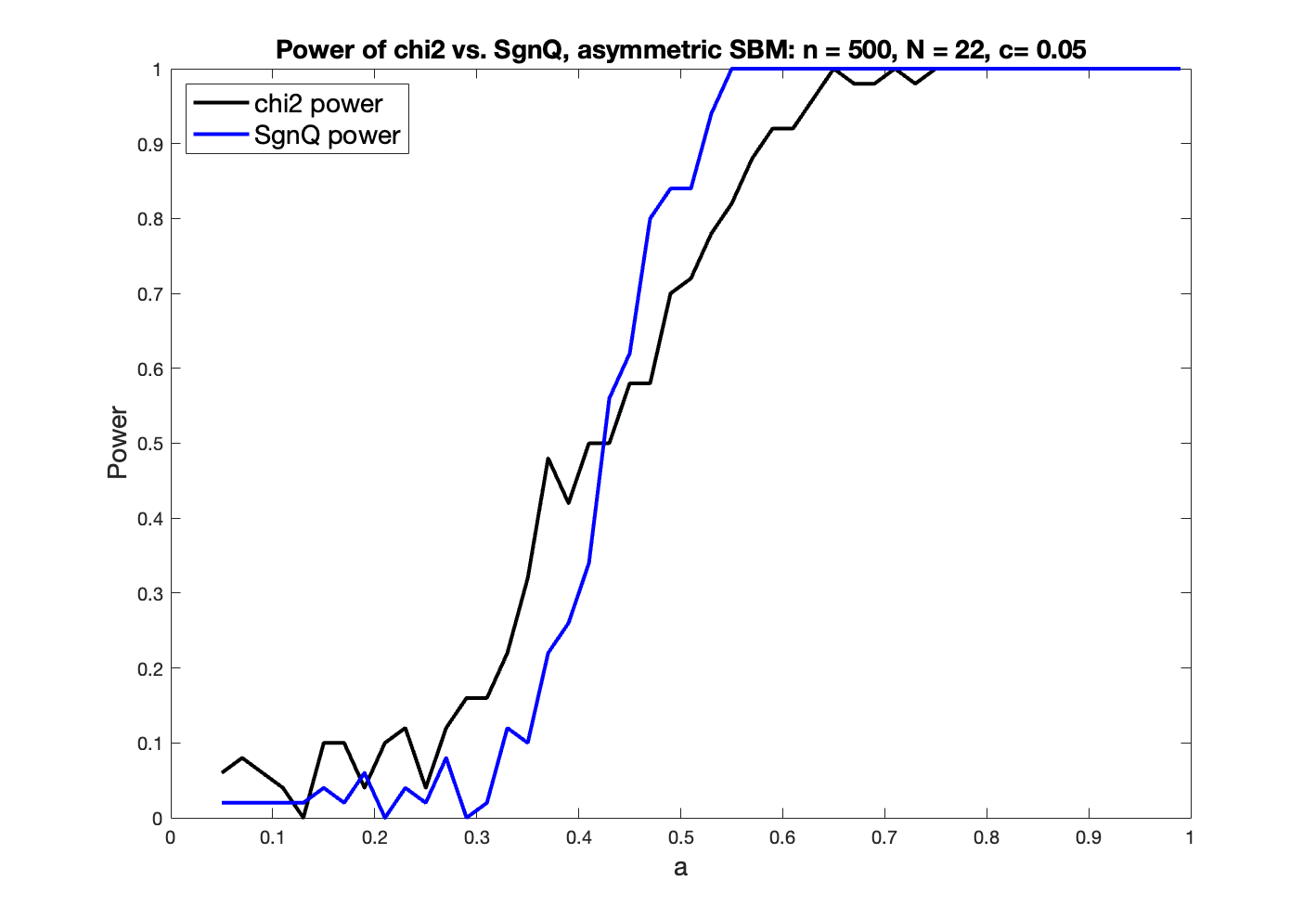
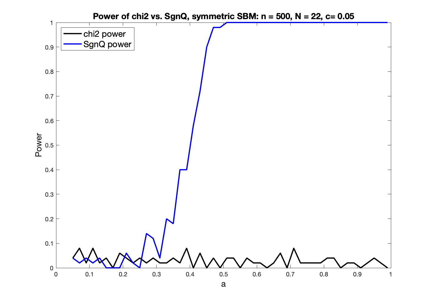
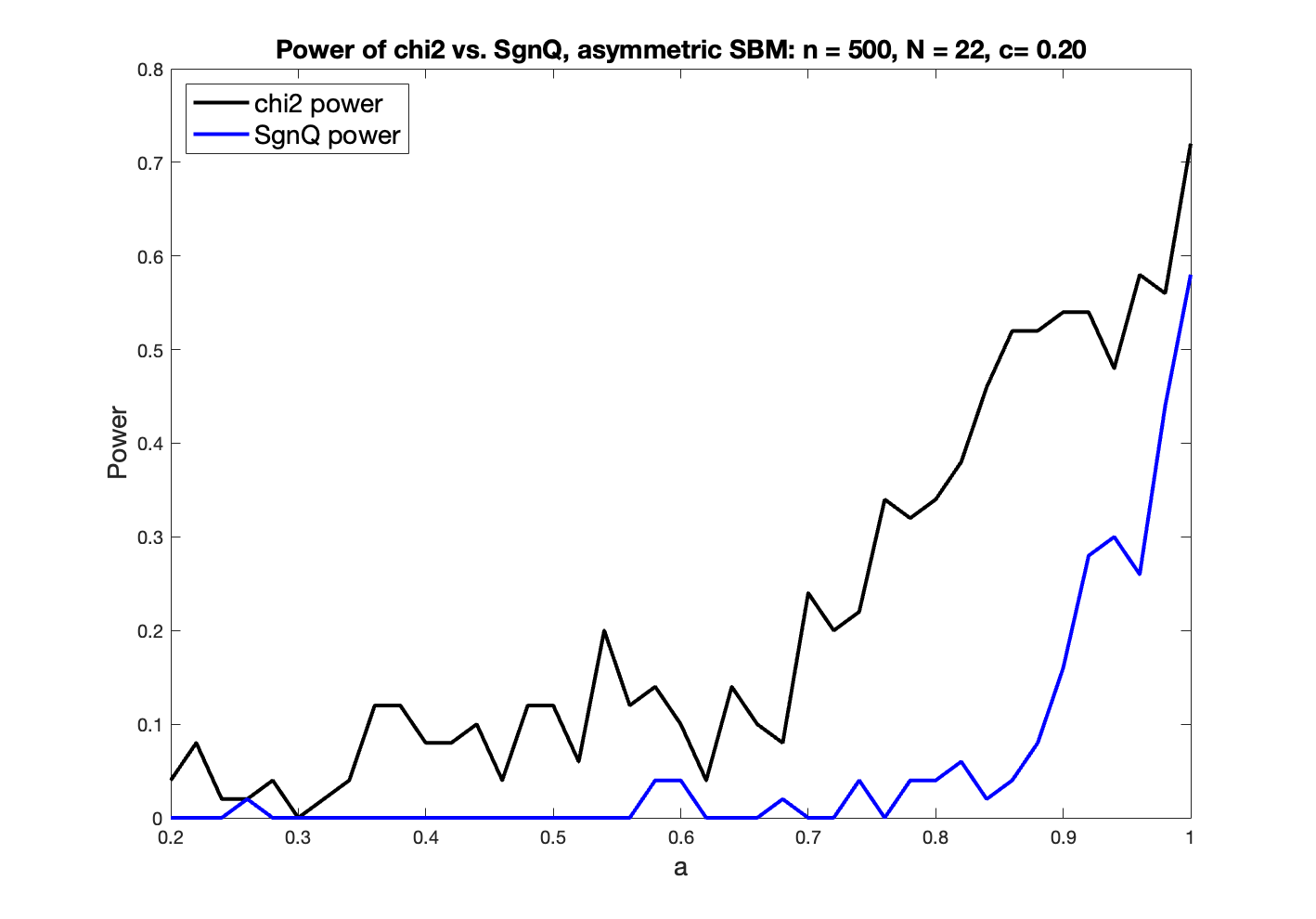
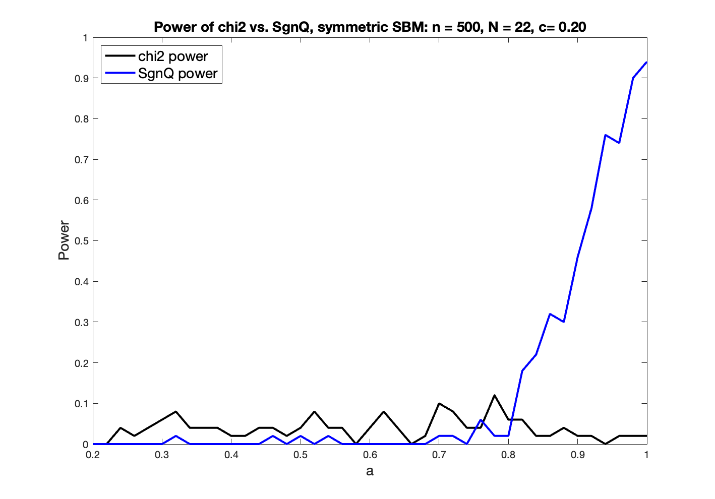
Figure 5: Power comparison of SgnQ and $\chi^{2}$ ($n=500$, $N=22$, 50 repetitions). We consider a 2-community SBM with $P_{11}=a$, $P_{22}=c$, $P_{12}=c$ (left) and $P_{12}=\frac{an-(a+c)N}{n}$ (right plot, the case of degree matching) where $c=0.05$ (top row) and $c=0.20$ (bottom row).

Appendix B Proof of Lemma 2.1 (Identifiability)

To prove identifiability, we make use of the following result from (Jin et al., 2021c, Lemma 3.1), which is in line with Sinkhorn’s work Sinkhorn (1974) on matrix scaling.

Lemma B.1 (Jin et al. (2021c)).

Given a matrix $A\in\mathbb{R}^{K,K}$ with strictly positive diagonal entries and non-negative off-diagonal entries, and a strictly positive vector $h\in\mathbb{R}^{K}$, there exists a unique diagonal matrix $D=\mathrm{diag}(d_{1},d_{2},\ldots,d_{K})$ such that $DADh=1_{K}$ and $d_{k}>0$, $1\leq k\leq K$.

We apply Lemma B.1 with $h=(h_{1},\ldots,h_{K})^{\prime}$ and $A=P$ to construct a diagonal matrix $D=\mathrm{diag}(d_{1},\ldots,d_{K})$ satisfying $DADh=1_{K}$. Note that $P$ has positive diagonal entries since $\Omega$ does.

Define $P^{*}=DPD$ and $D^{*}=\mathrm{diag}(d_{1}^{*},\ldots,d_{n}^{*})\in\mathbb{R}^{n}$ where

$$d_{i}^{*}\equiv d_{k}\qquad\text{if }i\in\mathcal{C}_{k}$$

Observe that

$$\Pi D^{-1}=(D^{*})^{-1}\Pi.$$

Define $\Theta^{*}=\Theta(D^{*})^{-1}$, and let $\theta^{*}=\mathrm{diag}(\Theta^{*})$. Next, let $\overline{\Theta}=\frac{n}{\|\theta^{*}\|_{1}}\cdot\Theta^{*}$, let $\overline{\theta}=\mathrm{diag}(\overline{\Theta})$, and let $\overline{P}=\frac{\|\theta^{*}\|_{1}^{2}}{n^{2}}\cdot P^{*}$. Note that $\|\overline{\theta}\|_{1}=n$ and $\overline{P}h\propto\mathbf{1}_{K}$.

Using the previous definitions and observations, we have

$$\Omega=\Theta\Pi D^{-1}DPDD^{-1}\Pi^{\prime}\Theta=\Theta^{*}\Pi P^{*}\Pi^{\prime}\Theta^{*}=\overline{\Theta}\Pi\overline{P}\Pi^{\prime}\overline{\Theta}$$

which justifies existence.

To justify uniqueness, suppose that

$$\Omega=\Theta^{(1)}\Pi P^{(1)}\Pi^{\prime}\Theta^{(1)}=\Theta^{(2)}\Pi P^{(2)}\Pi^{\prime}\Theta^{(2)},$$

where $\theta^{(i)}=\mathrm{diag}(\Theta^{(i)})$ satisfy $\|\theta^{(i)}\|_{1}=n$ for $i=1,2$ and

$$P^{(1)}h\propto\mathbf{1}_{K},\qquad P^{(2)}h\propto\mathbf{1}_{K}.$$

Observe that

$$\Pi P^{(1)}\Pi^{\prime}\mathbf{1}_{n}=\alpha^{(1)}n\cdot\mathbf{1}_{n},\qquad\Pi P^{(2)}\Pi^{\prime}\mathbf{1}_{n}=\alpha^{(2)}n\cdot\mathbf{1}_{n}.$$

for positive constants $\alpha^{(i)},i\in\{1,2\}$. Since $\Omega$ has nonnegative entries and positive diagonal elements, by Lemma B.1, there exists a unique diagonal matrix $D$ such that

$$D\Omega D\mathbf{1}_{n}=\mathbf{1}_{n}.$$

We see that taking $D=\frac{1}{\sqrt{\alpha^{(i)}n}}(\Theta^{(i)})^{-1}$ satisfies this equation for $i=1,2$, and therefore by uniqueness,

$$\frac{1}{\sqrt{\alpha^{(1)}n}}(\Theta^{(1)})^{-1}=\frac{1}{\sqrt{\alpha^{(2)}n}}(\Theta^{(2)})^{-1}.$$

Since $\|\theta^{(1)}\|_{1}=\|\theta^{(2)}\|_{1}=n$, further we have $\alpha^{(1)}=\alpha^{(2)}$, and hence

$$\Theta^{(1)}=\Theta^{(2)}.$$

It follows that

$$\Pi P^{(1)}\Pi^{\prime}=\Pi P^{(2)}\Pi^{\prime},$$

which, since we assume $h_{i}>0$ for $i=1,\ldots,K$, further implies that $P^{(1)}=P^{(2)}$. ∎

Appendix C Proof of Theorem 2.1 (Limiting null of the SgnQ statistic)

Consider a null DCBM with $\Omega=\theta^{*}(\theta^{*})^{\prime}$. Note that this is a different choice of parameterization than the one we study in the main paper. In (Jin et al., 2021c, Theorem 2.1) it is shown that the asymptotic distribution of $\psi_{n}$, the standardized version of SgnQ, is standard normal provided that

$$\|\theta^{*}\|\rightarrow\infty,\;\;\;\theta_{max}^{*}\rightarrow 0,\;\;\;\mbox{and}\;\;\;(\|\theta^{*}\|^{2}/\|\theta^{*}\|_{1})\sqrt{\log(\|\theta\|_{1}^{*})}\rightarrow 0.$$ (C.1)

We verify that, in a DCBM with $\Omega=\alpha\theta\theta^{\prime}$ and $\|\theta\|_{1}=n$, these conditions are implied by the assumptions in (2.5), restated below:

$$n\alpha\to\infty,\qquad\mbox{and}\qquad\alpha\theta^{2}_{\max}\log(n^{2}\alpha)\to 0$$ (C.2)

In the parameterization of Jin et al. (2021c), we have $\theta^{*}=\sqrt{\alpha}\theta$. First, $\|\theta^{*}\|^{2}\to\infty$ because by (C.2),

$$\|\theta^{*}\|^{2}\geq\frac{1}{n}\cdot\|\theta^{*}\|_{1}^{2}=\alpha n\to\infty.$$

Next, $\theta_{\max}^{*}\to 0$ because by (C.2),

$$\theta_{\max}=\sqrt{\alpha}\theta_{\max}\to 0.$$

To show the last part of (C.1), note that

$$(\|\theta^{*}\|^{2}/\|\theta^{*}\|_{1})\sqrt{\log(\|\theta\|_{1}^{*})}\leq\sqrt{\alpha}\theta_{\max}\sqrt{\log(\sqrt{\alpha}n)}=\frac{1}{\sqrt{2}}\sqrt{\alpha}\theta_{\max}\sqrt{\log(\alpha n^{2})}\to 0$$

by (C.2). Thus (C.1) holds, and $\psi_{n}$ is asymptotically standard normal under the null. ∎

Appendix D Proof of Lemma 2.2 (Properties of $\tilde{\Omega}$)

Lemma.

The rank and trace of the matrix $\widetilde{\Omega}$ are $(K-1)$ and $\|\theta\|^{2}\mathrm{diag}(\tilde{P})^{\prime}g$, respectively. When $K=2$, $\tilde{\lambda}_{1}=\mathrm{trace}(\widetilde{\Omega})=\|\theta\|^{2}(ac-b^{2})(d_{0}^{2}g_{1}+d_{1}^{2}g_{0})/(ad_{1}^{2}+2bd_{0}d_{1}+cd_{0}^{2})$.

Proof of Lemma 2.2. By basic algebra,

$$\widetilde{\Omega}=\Theta\Pi\widetilde{P}\Pi^{\prime}\Theta,\qquad\mbox{where $\widetilde{P}=(P-(d^{\prime}Pd)^{-1}Pdd^{\prime}P)$}.$$

It is seen $\widetilde{P}d=Pd-(d^{\prime}Pd)^{-1}Pdd^{\prime}Pd=0$, so $\mathrm{rank}(\widetilde{P})\leq K-1$. At the same time, since for any matrix $A$ and $B$ of the same size, $\mathrm{rank}(A+B)\leq\mathrm{rank}(A)+\mathrm{rank}(B)$, it follows $\widetilde{P}\geq(K-1)$, as $\mathrm{rank}(P)=K$ and $\mathrm{rank}(Pdd^{\prime}P)\leq 1$. This proves that $\mathrm{rank}(\widetilde{P})=K-1$.

At the same time, since for any matrices $A$ and $B$, $\mathrm{trace}(AB)=\mathrm{trace}(BA)$,

$$\mathrm{trace}(\widetilde{\Omega})=\mathrm{trace}(\widetilde{P}\Pi^{\prime}\Theta^{2}\Pi)=\|\theta\|^{2}\mathrm{trace}(\widetilde{P}G)=\|\theta\|^{2}\mathrm{diag}(\tilde{P})^{\prime}g.$$

This proves the second item of the lemma.

Last, when $K=2$, $\widetilde{\Omega}$ is rank $1$, and its eigenvalue is the same as its trace. First

$$(\tilde{P})_{11} =a-\frac{(ad_{1}+bd_{0})^{2}}{ad_{1}^{2}+2bd_{0}d_{1}+cd_{0}^{2}}=(ac-b^{2})\frac{d_{0}^{2}}{ad_{1}^{2}+2bd_{0}d_{1}+cd_{0}^{2}}$$

$$(\tilde{P})_{22} =c-\frac{(bd_{1}+cd_{0})^{2}}{ad_{1}^{2}+2bd_{0}d_{1}+cd_{0}^{2}}=(ac-b^{2})\frac{d_{1}^{2}}{ad_{1}^{2}+2bd_{0}d_{1}+cd_{0}^{2}}.$$

Thus

$$\tilde{\lambda}_{1}=\|\theta\|^{2}\mathrm{diag}(\tilde{P})^{\prime}g=\|\theta\|^{2}(ac-b^{2})\cdot\frac{d_{0}^{2}g_{1}+d_{1}^{2}g_{0}}{ad_{1}^{2}+2bd_{0}d_{1}+cd_{0}^{2}}$$

This proves the last item and completes the proof of the lemma.

∎

Appendix E Proof of Theorem 2.2 (Power of the SgnQ test) and Corollary 2.1

E.1 Setup and results

Notation: Given sequences of real numbers $A=A_{n}$ and $B=B_{n}$, we write $A\lesssim B$ to signify that $A=O(B)$, $A\asymp B$ to signify that $A\lesssim B$ and $B\lesssim A$, and $A\sim B$ to signify that $A/B=1+o(1)$.

Throughout this section, we consider a DCBM with parameters $(\Theta,P)$ where $P\in\mathbb{R}^{2\times 2}$ has unit diagonals, and we analyze the behavior of SgnQ under the alternative. At the end of this subsection we explain how Theorem 2.2 and Corollary 2.1 follow from the results described next. Our results hinge on

$$\tilde{\lambda}\equiv\tilde{\lambda}_{1}=\mathrm{tr}(\tilde{\Omega}).$$

Given a subset $U\subset[n]$, let $\theta_{U}\in\mathbb{R}^{|U|}$ denote the restriction of $\theta$ to the coordinates of $U$. For notational convenience, we let $S=\{i:\pi_{i}(1)=1\}$, which was previously written as $\mathcal{C}_{1}$ in the main paper.

In a DCBM where $P$ has unit diagonals, our main results hold under the following conditions.

$$\Omega_{ij} \lesssim\theta_{i}\theta_{j}$$ (E.1)

$$\|\theta\|_{\infty} =O(1),\text{ and }$$ (E.2)

$$\|\theta\|_{2}^{2} \to\infty.$$ (E.3)

$$(\|\theta\|_{2}^{2}/\|\theta\|_{1})\sqrt{\log(\|\theta\|_{1})} \to 0.$$ (E.4)

First we justify that these assumptions are satisfied by an equivalent DCBM with the same $\Omega$ represented with the parameterization (2.1) and satisfying (2.7). Thus all results proved in this section transfer immediately to the main paper.

Lemma E.1.

Consider a DCBM with parameters $(\Theta^{*},P^{*})$ satisfying (2.1) and satisfying (2.7). Define $\Theta=\mathrm{diag}(\theta)$ where

$$\theta_{i}=\begin{cases}\sqrt{a}\theta_{i}^{*}&\quad\text{if }i\in S\\ \sqrt{c}\theta_{i}^{*}&\quad\text{if }i\in S^{c},\end{cases}$$

and

$$P=\begin{pmatrix}1&\frac{b}{\sqrt{ac}}\\ \frac{b}{\sqrt{ac}}&1\end{pmatrix}.$$

Then

$$\Omega=\Theta\Pi P\Pi\Theta=\Theta^{*}\Pi P^{*}\Pi^{\prime}\Theta^{*}$$

and (E.1)–(E.4) are satisfied.

Proof.

The statement regarding $\Omega$ follows by basic algebra. (E.1) follows if we can show that

$$\frac{b}{\sqrt{ac}}\lesssim 1.$$ (E.5)

Since

$$b=\frac{cn-(a+c)N}{n-2N}=c\cdot\frac{n-N}{n-2N}-a\cdot\frac{N}{n-2N},$$

we have $a\geq c\gtrsim b$, so (E.5) follows.

Next, (E.2) follows directly from $a\theta_{\max,1}^{2}\lesssim 1$ since $c\theta_{\max,0}^{2}=o(1)$ by (2.7).

For (E.3),

$$\|\theta\|_{2}^{2}\geq\frac{1}{n}\cdot\|\theta\|_{1}^{2}\geq cn\to\infty$$

by (2.7).

For the last part, note that

$$b=c\cdot\frac{n-N}{n-2N}-a\cdot\frac{N}{n-2N}\geq 0\Rightarrow a\varepsilon\lesssim c.$$

Thus,

$$\frac{\|\theta\|_{2}^{2}}{\|\theta\|_{1}} =\frac{a\|\theta_{S}^{*}\|_{2}^{2}+c\|\theta_{S^{c}}^{*}\|_{2}^{2}}{\sqrt{a}\|\theta_{S}^{*}\|_{1}+\sqrt{c}\|\theta_{S^{c}}^{*}\|_{1}}\lesssim\frac{a(N/n)\|\theta^{*}_{S^{c}}\|_{2}^{2}+c\|\theta_{S^{c}}^{*}\|_{2}^{2}}{\sqrt{c}\|\theta^{*}_{S^{c}}\|_{1}}$$

$$\lesssim\frac{c\|\theta_{S^{c}}^{*}\|_{2}^{2}}{\sqrt{c}\|\theta_{S^{c}}^{*}\|_{1}}\lesssim\sqrt{c}\theta_{\max,0}=o\big{(}\frac{1}{\sqrt{\log cn^{2}}}\big{)}=o\big{(}\frac{1}{\sqrt{\log(\|\theta\|_{1}})}\big{)},$$

which implies (E.4). Above we use that $a\geq c$ and $g_{1}\asymp d_{1}\asymp N/n$, by assumption. Precisely, in the first line, we used

$$a\|\theta^{*}_{S}\|_{2}^{2}\asymp a\cdot(1-N/n)^{-1}\frac{N}{n}\|\theta^{*}_{S^{c}}\|_{2}^{2}\lesssim c\|\theta^{*}_{S^{c}}\|_{2}^{2},$$

and in the second line we used

$$\|\theta\|_{1} \geq\sqrt{c}\|\theta_{S^{c}}^{*}\|_{1}\asymp\sqrt{c}(1-N/n)^{-1}\|\theta^{*}\|_{1}\asymp\sqrt{c}n.$$

∎

With Lemma E.1 in hand, we restrict in the remainder of this section to the setting where $P$ has unit diagonals and (E.1)–(E.4) are satisfied.

Define $v_{0}=\mathbf{1}^{\prime}\Omega\mathbf{1}$, and let $\eta^{*}=(1/\sqrt{v_{0}})\Omega\mathbf{1}$. Recall $\tilde{\Omega}=\Omega-\eta^{*}\eta^{*\mathsf{T}}$, and $\tilde{\lambda}=\mathrm{tr}(\tilde{\Omega})$. Our main result concerning the alternative is the following.

Theorem E.1 (Limiting behavior of SgnQ test statistic).

Suppose that the previous assumptions hold and that $|\tilde{\lambda}|/\sqrt{\lambda_{1}}\to\infty$. Then under the null hypothesis, as $n\to\infty$, $\mathbb{E}[Q]\sim 2\|\theta\|_{2}^{4}$, $\mathrm{Var}(Q)\sim 8\|\theta\|_{2}^{8}$, and $(Q-\mathbb{E}Q)/\sqrt{\mathrm{Var}(Q)}\to N(0,1)$ in law. Under the alternative hypothesis, as $n\to\infty$, $\mathbb{E}Q\sim\tilde{\lambda}^{4}$ and $\mathrm{Var}(Q)\lesssim|\tilde{\lambda}|^{6}+|\tilde{\lambda}|^{2}\lambda_{1}^{3}=o(\tilde{\lambda}^{8})$.

Following Jin et al. (2021c), we introduce some notation:

$$\widetilde{\Omega}=\Omega-(\eta^{*})(\eta^{*})^{\prime},\qquad\mbox{where}\quad\eta^{*}=\frac{1}{\sqrt{v_{0}}}\Omega{\bf 1}_{n},\;\;v_{0}={\bf 1}_{n}^{\prime}\Omega{\bf 1}_{n};$$

$$\delta_{ij}=\eta_{i}(\eta_{j}-\tilde{\eta}_{j})+\eta_{j}(\eta_{i}-\tilde{\eta}_{i}),\qquad\mbox{where}\quad\eta=\frac{1}{\sqrt{v}}(\mathbb{E}A){\bf 1}_{n},\;\;\tilde{\eta}=\frac{1}{\sqrt{v}}A{\bf 1}_{n},\;\;v={\bf 1}_{n}^{\prime}(\mathbb{E}A){\bf 1}_{n};$$

$$r_{ij}=(\eta_{i}^{*}\eta_{j}^{*}-\eta_{i}\eta_{j})-(\eta_{i}-\tilde{\eta}_{i})(\eta_{j}-\tilde{\eta}_{j})+(1-\frac{v}{V})\tilde{\eta}_{i}\tilde{\eta}_{j},\qquad\mbox{where}\;\;V={\bf 1}_{n}^{\prime}A{\bf 1}_{n}.$$

The ideal and proxy SgnQ statistics, respectively, are defined as follows:

$$\widetilde{Q}_{n} =\sum_{i,j,k,\ell(dist)}(\widetilde{\Omega}_{ij}+W_{ij})(\widetilde{\Omega}_{jk}+W_{jk})(\widetilde{\Omega}_{k\ell}+W_{k\ell})(\widetilde{\Omega}_{\ell i}+W_{\ell i})$$ (E.6)

$$Q_{n}^{*} =\sum_{i,j,k,\ell(dist)}(\widetilde{\Omega}_{ij}+W_{ij}+\delta_{ij})(\widetilde{\Omega}_{jk}+W_{jk}+\delta_{jk})(\widetilde{\Omega}_{k\ell}+W_{k\ell}+\delta_{k\ell})(\widetilde{\Omega}_{\ell i}+W_{\ell i}+\delta_{\ell i}).$$ (E.7)

Moreover, we can express the original or real SgnQ as

$$Q_{n}=\sum_{i,j,k,\ell(dist)}\bigg{[}(\widetilde{\Omega}_{ij}+W_{ij}+\delta_{ij}+r_{ij}) (\widetilde{\Omega}_{jk}+W_{jk}+\delta_{jk}+r_{jk})$$

$$(\widetilde{\Omega}_{k\ell}+W_{k\ell}+\delta_{k\ell}+r_{k\ell})(\widetilde{\Omega}_{\ell i}+W_{\ell i}+\delta_{\ell i}+r_{\ell i})\bigg{]}.$$

The next theorems handle the behavior of these statistics. Together the results imply Theorem E.1. Again, the analysis of the null carries over directly from Jin et al. (2021c), so we only need to study the alternative. The claims regarding the alternative follow from Lemmas E.7–E.12 below.

Theorem E.2 (Ideal SgnQ test statistic).

Suppose that the previous assumptions hold and that $|\tilde{\lambda}|/\sqrt{\lambda_{1}}\to\infty$. Then under the null hypothesis, as $n\to\infty$, $\mathbb{E}[\tilde{Q}]=0$ and $\mathrm{Var}(\tilde{Q})=8\|\theta\|_{2}^{8}\cdot[1+o(1)]$. Furthermore, under the alternative hypothesis, as $n\to\infty$, $\mathbb{E}[\tilde{Q}]\sim\tilde{\lambda}^{4}$ and $\mathrm{Var}(\tilde{Q})\lesssim\lambda_{1}^{4}+|\tilde{\lambda}|^{6}=o(\tilde{\lambda}^{8})$.

Theorem E.3 (Proxy SgnQ test statistic).

Suppose that the previous assumptions hold and that $|\tilde{\lambda}|/\sqrt{\lambda_{1}}\to\infty$. Then under the null hypothesis, as $n\to\infty$, $|\mathbb{E}[\tilde{Q}-Q^{*}]|=o(\|\theta\|_{2}^{4})$ and $\mathrm{Var}(\tilde{Q}-Q^{*})=o(\|\theta\|_{2}^{8})$. Furthermore, under the alternative hypothesis, as $n\to\infty$, $|\mathbb{E}[\tilde{Q}-Q^{*}]|\lesssim|\tilde{\lambda}|^{2}\lambda_{1}=o(\tilde{\lambda}^{4})$ and $\mathrm{Var}(\tilde{Q}-Q^{*})\lesssim|\tilde{\lambda}|^{2}\lambda_{1}^{3}+|\tilde{\lambda}|^{6}=o(\tilde{\lambda}^{8})$.

Theorem E.4 (Real SgnQ test statistic).

Suppose that the previous assumptions hold and that $|\tilde{\lambda}|/\sqrt{\lambda_{1}}\to\infty$. Then under the null hypothesis, as $n\to\infty$, $|\mathbb{E}[Q-\tilde{Q}]|=o(\|\theta\|_{2}^{4})$ and $\mathrm{Var}(Q-\tilde{Q})=o(\|\theta\|_{2}^{8})$. Furthermore, under the alternative hypothesis, as $n\to\infty$, $|\mathbb{E}[Q-Q^{*}]|\lesssim|\tilde{\lambda}|^{2}\lambda_{1}=o(\tilde{\lambda}^{4})$ and $\mathrm{Var}(Q-Q^{*})\lesssim|\tilde{\lambda}|^{2}\lambda_{1}^{3}=o(\tilde{\lambda}^{8})$.

The previous work Jin et al. (2021c) establishes that under the assumptions above, if $\|\theta_{S}\|_{1}/\|\theta\|_{1}\asymp 1$, then SgnQ distinguishes the null and alternative provided that $|\lambda_{2}|/\sqrt{\lambda_{1}}\to\infty$. To compare with the results above, note that $\lambda_{2}\asymp\tilde{\lambda}$ if $\|\theta_{S}\|_{1}/\|\theta\|_{1}\asymp 1$ (c.f. Lemma E.5 of Jin et al. (2021c)). Thus when $K=2$, our main result extends the upper bound of Jin et al. (2021c) to the case when $\|\theta_{S}\|_{1}/\|\theta\|_{1}=o(1)$. We note that $|\tilde{\lambda}|\gtrsim|\lambda_{2}|$ in general (see Lemma E.3 and Corollary E.1).

The theorems above apply to the symmetric SBM. Recall that in this model,

$$\Omega_{ij}=\begin{cases}a&\quad\text{ if }i,j\in S\\ c&\quad\text{ if }i,j\notin S\\ \tilde{b}=\frac{nc-(a+c)N}{n-2N}&\quad\text{ otherwise. }\end{cases}$$

where $N=|S|$ and $a,b,c\in(0,1)$. To obtain this model from our DCBM, set

$$P=\begin{pmatrix}1&\tilde{b}/\sqrt{ac}\\ \tilde{b}/\sqrt{ac}&1\\ \end{pmatrix},$$ (E.8)

and

$$\theta=\sqrt{a}\mathbf{1}_{S}+\sqrt{c}\mathbf{1}_{S^{c}}.$$ (E.9)

The assumption (E.1) implies that $\tilde{b}\lesssim\sqrt{ac}$, which is automatically satisfied since we assume $a\geq c$.

In SBM, it holds that $\lambda_{2}=\tilde{\lambda}$ (see Lemma E.3). Furthermore, explicit calculations in Section E.5 reveal that

$$\lambda_{1} \sim nc,\text{ and }$$ (E.10)

$$\lambda_{2} =\tilde{\lambda}\sim N(a-c).$$

In addition, with $P,a,\tilde{b},c$ as above, if we have

$$\theta_{i}=\begin{cases}\rho_{i}\sqrt{a}&\qquad\text{if }i\in S\\ \rho_{i}\sqrt{c}&\qquad\text{if }i\notin S\end{cases}$$

for $\rho>0$ with $\rho_{\min}\gtrsim\rho_{\max}$ in the DCBM setting, a very similar calculation, which we omit, reveals that

$$\lambda_{1} \asymp nc,\text{ and }$$ (E.11)

$$\tilde{\lambda} \asymp N(a-c).$$

With the previous results of this subsection in hand (which are proved in the remaining subsections) we justify Theorem 2.2 and Corollary 2.1.

Proof of Theorem 2.2.

The SgnQ test has level $\kappa$ by Theorem 2.1, so it remains to study the type II error. Using Theorem E.1 and Lemma E.1, the fact that the type II error tends to $0$ directly follows from Chebyshev’s inequality and the fact that $\|\hat{\eta}\|_{2}^{2}-1\approx\|\theta\|_{2}^{2}$ with high probability. In particular, note that since $|\tilde{\lambda}|\gg\sqrt{\lambda_{1}}$, the expectation of SgnQ under the alternative is much larger than its standard deviation, under the null or alternative. We omit the details as they are very similar to the proof of Theorem 2.6 in (Jin et al., 2021c, Supplement,pgs. 5–6). ∎

Proof of Corollary 2.1.

This result follows immediately from (E.11) and Theorem 2.2. ∎

E.2 Preliminary bounds

Define $v_{0}=\mathbf{1}^{\mathsf{T}}\Omega\mathbf{1}$, and let $\eta^{*}=1/\sqrt{v_{0}}\cdot\Omega\mathbf{1}$. For the analysis of SgnQ, it is important is to understand $\tilde{\Omega}=\Omega-\eta^{*}\eta^{*\mathsf{T}}$. The next lemma establishes that $\tilde{\Omega}$ is rank one and has a simple expression when $K=2$.

Lemma E.2.

Let $f=(\|\theta_{S^{c}}\|_{1},-\|\theta_{S}\|_{1})^{\mathsf{T}}$ It holds that

$$\tilde{\Omega}=\frac{(1-b^{2})}{v_{0}}\cdot\Theta\Pi ff^{\mathsf{T}}\Pi^{\mathsf{T}}\Theta.$$

Proof.

Let $\rho_{0}=\|\theta_{S}\|_{1}$ and $\rho_{1}=\|\theta_{S^{c}}\|_{1}$. Note that

$$(\Omega\mathbf{1})_{i}=\theta_{i}\sum_{j}\theta_{j}\pi_{i}^{\mathsf{T}}P\pi_{j}=\begin{cases}\theta_{i}(\rho_{0}+b\rho_{1})&\quad\text{ if }i\in S\\ \theta_{i}(b\rho_{0}+\rho_{1})&\quad\text{ if }i\notin S.\end{cases}$$

Hence

$$v_{0}=\mathbf{1}^{\mathsf{T}}\Omega\mathbf{1}=\rho_{0}^{2}+2b\rho_{0}\rho_{1}+\rho_{1}^{2}.$$

If $i,j\in S$, then

$$\tilde{\Omega}_{ij}=\theta_{i}\theta_{j}\big{(}1-\frac{(\rho_{0}+b\rho_{1})^{2}}{v_{0}}\big{)}=\theta_{i}\theta_{j}\cdot\frac{(1-b^{2})\rho_{1}^{2}}{v_{0}}$$

Similarly if $i\in S$ and $j\notin S$,

$$\tilde{\Omega}_{ij}=\theta_{i}\theta_{j}\big{(}b-\frac{(\rho_{0}+b\rho_{1})(b\rho_{0}+\rho_{1})}{v_{0}}\big{)}=-\theta_{i}\theta_{j}\cdot\frac{(1-b^{2})\rho_{0}\rho_{1}}{v_{0}}$$

and

$$\tilde{\Omega}_{ij}=\theta_{i}\theta_{j}\big{(}1-\frac{(b\rho_{0}+\rho_{1})^{2}}{v_{0}}\big{)}=\theta_{i}\theta_{j}\cdot\frac{(1-b^{2})\rho_{0}^{2}}{v_{0}}$$

if $i,j\in S^{c}$. The claim follows. ∎

Let

$$w=\Theta\Pi f=\theta_{S}\|\theta_{S^{c}}\|_{1}-\theta_{S^{c}}\|\theta_{S}\|_{1}=\rho_{1}\theta_{S}-\rho_{0}\theta_{S^{c}}$$

Using the previous lemma, we have the rank one eigendecomposition

$$\tilde{\Omega}=\tilde{\lambda}\tilde{\xi}\tilde{\xi}^{\mathsf{T}},$$ (E.12)

where we define

$$\tilde{\xi} =\frac{\rho_{1}\theta_{S}-\rho_{0}\theta_{S^{c}}}{\|\rho_{1}\theta_{S}-\rho_{0}\theta_{S^{c}}\|_{2}}=\frac{\rho_{1}\theta_{S}-\rho_{0}\theta_{S^{c}}}{\sqrt{\rho_{1}^{2}\|\theta_{S}\|_{2}^{2}+\rho_{0}^{2}\|\theta_{S^{c}}\|_{2}^{2}}},\text{ and }$$ (E.13)

$$\tilde{\lambda} =\frac{(1-b^{2})}{v_{0}}\cdot\big{(}\rho_{1}^{2}\|\theta_{S}\|_{2}^{2}+\rho_{0}^{2}\|\theta_{S^{c}}\|_{2}^{2}\big{)}.$$ (E.14)

Lemma E.5 of Jin et al. (2021c) implies that if $\|\theta_{S}\|_{1}/\|\theta\|_{1}\asymp 1$, then $\lambda_{2}\asymp\tilde{\lambda}_{1}$ . If $\|\theta_{S}\|_{1}/\|\theta\|_{1}=o(1)$, then this guarantee may not hold. Below, in the case $K=2$, we express $\tilde{\lambda}$ in terms of the eigenvalues and eigenvectors of $\Omega$. This allows us to compare $\lambda_{2}$ with $\tilde{\lambda}$ more generally, as in Corollary E.1.

Lemma E.3.

Let $\Omega$ have eigenvalues $\lambda_{1},\lambda_{2}$ and eigenvectors $\xi_{1},\xi_{2}$. Let $\tilde{\lambda}$ denote the eigenvalue of $\tilde{\Omega}$. Then

$$\tilde{\lambda}=\frac{\lambda_{1}\lambda_{2}\big{(}\langle\xi_{1},\mathbf{1}\rangle^{2}+\langle\xi_{2},\mathbf{1}\rangle^{2}\big{)}}{\lambda_{1}\langle\xi_{1},\mathbf{1}\rangle^{2}+\lambda_{2}\langle\xi_{2},\mathbf{1}\rangle^{2}}.$$ (E.15)

Proof.

By explicit computation,

$$\tilde{\Omega} =\Omega-\eta^{*}\eta^{*\mathsf{T}}$$

$$=\lambda_{1}\big{(}1-\frac{\lambda_{1}\langle\xi_{1},\mathbf{1}\rangle^{2}}{v_{0}}\big{)}\xi_{1}\xi_{1}^{\mathsf{T}}+\lambda_{2}\big{(}1-\frac{\lambda_{2}\langle\xi_{2},\mathbf{1}\rangle^{2}}{v_{0}}\big{)}\xi_{2}\xi_{2}^{\mathsf{T}}-\frac{\lambda_{1}\lambda_{2}\langle\xi_{1},\mathbf{1}\rangle\langle\xi_{2},\mathbf{1}\rangle}{v_{0}}\big{(}\xi_{1}\xi_{2}^{\mathsf{T}}\xi_{2}+\xi_{1}^{\mathsf{T}}\big{)}$$

$$=\frac{\lambda_{1}\lambda_{2}}{v_{0}}\,\big{(}\langle\xi_{2},\mathbf{1}\rangle\xi_{1}+\langle\xi_{1},\mathbf{1}\rangle\xi_{2}\big{)}\cdot\big{(}\langle\xi_{2},\mathbf{1}\rangle\xi_{1}+\langle\xi_{1},\mathbf{1}\rangle\xi_{2}\big{)}^{\mathsf{T}}.$$

From (E.13) and (E.14), it follows that

$$\tilde{\xi} =\frac{\langle\xi_{2},\mathbf{1}\rangle\xi_{1}+\langle\xi_{1},\mathbf{1}\rangle\xi_{2}}{\sqrt{\langle\xi_{1},\mathbf{1}\rangle^{2}+\langle\xi_{2},\mathbf{1}\rangle^{2}}}$$

$$\tilde{\lambda} =\frac{\lambda_{1}\lambda_{2}}{v_{0}}\big{(}\langle\xi_{1},\mathbf{1}\rangle^{2}+\langle\xi_{2},\mathbf{1}\rangle^{2}\big{)}.$$

∎

Corollary E.1.

It holds that

$$|\lambda_{2}|\lesssim|\tilde{\lambda}|\lesssim\lambda_{1}.$$ (E.16)

If $\lambda_{2}\geq 0$, then

$$\lambda_{2}\leq\tilde{\lambda}\leq\lambda_{1}$$ (E.17)

Proof.

Suppose that $\lambda_{2}\geq 0$. Then

$$\lambda_{2}\big{(}\langle\xi_{1},\mathbf{1}\rangle^{2}+\langle\xi_{2},\mathbf{1}\rangle^{2}\big{)}\leq\lambda_{1}\langle\xi_{1},\mathbf{1}\rangle^{2}+\lambda_{2}\langle\xi_{2},\mathbf{1}\rangle^{2}=v_{0}\leq\lambda_{1}\big{(}\langle\xi_{1},\mathbf{1}\rangle^{2}+\langle\xi_{2},\mathbf{1}\rangle^{2}\big{)},$$

implies (E.17).

Suppose that $\lambda_{2}<0$. Note that

$$\lambda_{1}\big{(}\langle\xi_{1},\mathbf{1}\rangle^{2}+\langle\xi_{2},\mathbf{1}\rangle^{2}\big{)}\geq\lambda_{1}\langle\xi_{1},\mathbf{1}\rangle^{2}+\lambda_{2}\langle\xi_{2},\mathbf{1}\rangle^{2}=v_{0}\geq 0,$$

which combined with (E.15) implies that $|\tilde{\lambda}|\geq|\lambda_{2}|$.

Next,

$$\lambda_{2} \leq\tilde{\xi}^{\mathsf{T}}\Omega\tilde{\xi}=\tilde{\lambda}+\langle\tilde{\xi},\eta^{*}\rangle^{2},$$

which implies that

$$|\tilde{\lambda}|\leq|\lambda_{2}|+\langle\tilde{\xi},\eta^{*}\rangle^{2}\leq\lambda_{1}+\|\eta^{*}\|_{2}^{2}\lesssim\lambda_{1}+\|\theta\|_{1}^{2}\lesssim\lambda_{1},$$

where the last inequality follows from Lemma E.5. ∎

The next results are frequently used in our analyis of SgnQ.

Lemma E.4.

Let $v=\mathbf{1}^{\mathsf{T}}(\Omega-\mathrm{diag}(\Omega))\mathbf{1}$ and $v_{0}=\mathbf{1}^{\mathsf{T}}\Omega\mathbf{1}$. Then

$$v_{0}\sim v\sim\|\theta\|_{1}^{2}.$$ (E.18)

Proof.

By (E.4), $\|\theta\|_{2}^{2}=o(\|\theta\|_{1})$. By (E.3), $\|\theta\|_{1}\to\infty$. Hence

$$v=\mathbf{1}^{\mathsf{T}}(\Omega-\mathrm{diag}(\Omega))\mathbf{1}=\|\theta\|_{1}^{2}-\|\theta\|_{2}^{2}\sim\|\theta\|_{1}^{2}\sim v_{0}=\mathbf{1}^{\mathsf{T}}\Omega\mathbf{1}.$$

∎

The next result is a direct corollary of Lemmas E.2 and E.4.

Corollary E.2.

Define $\beta\in\mathbb{R}^{n}$ by

$$\beta=\sqrt{\frac{|1-b^{2}|}{v_{0}}}\cdot\big{(}\|\theta_{S^{c}}\|_{1}\mathbf{1}_{S}+\|\theta_{S}\|_{1}\mathbf{1}_{S^{c}}\big{)}$$ (E.19)

Then

$$|\tilde{\Omega}_{ij}|\lesssim\beta_{i}\theta_{i}\beta_{j}\theta_{j}.$$ (E.20)

Lemma E.5.

Let $\lambda_{1}$ denote the largest eigenvalue of $\Omega$. Then

$$\lambda_{1}\gtrsim\|\theta\|_{2}^{2}.$$ (E.21)

Proof.

Using the universal inequality $a^{2}+b^{2}\geq\frac{1}{2}(a+b)^{2}$, we have

$$\lambda_{1} \geq\frac{\theta^{\mathsf{T}}\Omega\theta}{\|\theta\|_{2}^{2}}\geq\frac{1}{\|\theta\|_{2}^{2}}\cdot\sum_{i,j}\theta_{i}\theta_{j}\Omega_{ij}\geq\frac{1}{\|\theta\|_{2}^{2}}\cdot\big{(}\sum_{i,j\in S}\theta_{i}^{2}\theta_{j}^{2}+\sum_{i,j\notin S}\theta_{i}^{2}\theta_{j}^{2}\big{)}$$

$$\geq\frac{\|\theta_{S}\|_{2}^{4}+\|\theta_{S^{c}}\|_{2}^{4}}{\|\theta\|_{2}^{2}}\gtrsim\|\theta\|_{2}^{2}.$$

∎

Lemma E.6.

Define $\eta=\frac{1}{\sqrt{v}}(\Omega-\mathrm{diag}(\Omega))\mathbf{1}$. Then

$$\eta_{i}\lesssim\eta_{i}^{*}\lesssim\theta_{i}$$ (E.22)

Proof.

The left-hand side is immediate, so we prove that $\eta_{i}^{*}\lesssim\theta_{i}$. We have

$$(\Omega\mathbf{1})_{i}=\begin{cases}\theta_{i}(\|\theta_{S}\|_{1}+b\|\theta_{S^{c}}\|_{1})\quad\text{if }i\in S\\ \theta_{i}(b\|\theta_{S}\|_{1}+\|\theta_{S^{c}}\|_{1})\quad\text{if }i\notin S\end{cases}$$

Since $\Omega_{ii}=\theta_{i}^{2}$,

$$\sqrt{v_{0}}\cdot\eta_{i}=\begin{cases}\theta_{i}(\|\theta_{S}\|_{1}+b\|\theta_{S^{c}}\|_{1})-\theta_{i}^{2}\quad\text{if }i\in S\\ \theta_{i}(b\|\theta_{S}\|_{1}+\|\theta_{S^{c}}\|_{1})-\theta_{i}^{2}\quad\text{if }i\notin S.\end{cases}$$

Since $b=O(1)$, $\theta_{i}=O(1)$, and $v_{0}\gtrsim\|\theta\|_{1}^{2}$ (c.f. Lemma E.4),

$$\eta_{i}^{*}\lesssim\frac{\theta_{i}\|\theta\|_{1}}{\sqrt{\|\theta\|_{1}^{2}}}=\theta_{i},$$

as desired. ∎

We use the bounds (E.18) – (E.22) throughout. We also use repeatedly that

$$\|\theta\|_{p}^{p} \lesssim\|\theta\|_{q}^{q},\text{ if }p\geq q,$$ (E.23)

which holds by (E.2), and

$$\|\beta\circ\theta\|_{2}^{2} =|\tilde{\lambda}|$$

$$|\beta_{i}| \lesssim 1$$

$$\|\beta\circ\theta^{\circ 2}\|_{1} \leq\|\beta\circ\theta\|_{2}\|\theta\|_{2}\lesssim\|\theta\|_{2}^{2},$$ (E.24)

where the second line holds by Cauchy–Schwarz.

E.3 Mean and variance of SgnQ

The previous work Jin et al. (2021c) decomposes $\tilde{Q}$ and $\tilde{Q}-Q^{*}$ into a finite number of terms. For each term an exact expression for its mean and variance is derived in Jin et al. (2021c) that depends on $\theta$, $\eta$, $v$, and $\tilde{\Omega}$. These expression are then bounded using the inequalities (E.2), (E.3), (E.18), (E.21)–(E.23), as well as an inequality of the form

$$|\tilde{\Omega}_{ij}|\lesssim\alpha\theta_{i}\theta_{j}.$$

In our case, an inequality of this form is still valid, but it does not attain sharp results because it does not properly capture the signal $|\tilde{\lambda}|$ from the smaller community. Instead, we use the inequality (E.20), followed by the bounds in (E.24) to handle terms involving $\tilde{\Omega}$.

Therefore, for terms of $\tilde{Q}$ and $\tilde{Q}-Q^{*}$ that do not depend on $\tilde{\Omega}$, the bounds in Jin et al. (2021c) carry over immediately. In particular, their analysis of the null hypothesis carries over directly. Hence we can focus solely on the alternative hypothesis.

Furthermore, any terms with zero mean in Jin et al. (2021c) also have zero mean in our setting : for every term that is mean zero, it is simply the sum of mean zero subterms, and each mean zero subterm is a product of independent, centered random variables (eg, $X_{1}$ below).

E.3.1 Ideal SgnQ

The previous work Jin et al. (2021c) shows that $\tilde{Q}=X_{1}+4X_{2}+4X_{3}+2X_{4}+4X_{5}+X_{6}$, where $X_{1},\ldots,X_{6}$ are defined in their Section G.1. For convenience, we state explicitly the definitions of these terms.

$$X_{1}=\sum_{i,j,k,\ell(dist)}W_{ij}W_{jk}W_{k\ell}W_{\ell i},\qquad X_{2}=\sum_{i,j,k,\ell(dist)}\widetilde{\Omega}_{ij}W_{jk}W_{k\ell}W_{\ell i},$$

$$X_{3}=\sum_{i,j,k,\ell(dist)}\widetilde{\Omega}_{ij}\widetilde{\Omega}_{jk}W_{k\ell}W_{\ell i},\qquad\;X_{4}=\sum_{i,j,k,\ell(dist)}\widetilde{\Omega}_{ij}W_{jk}\widetilde{\Omega}_{k\ell}W_{\ell i},$$

$$X_{5}=\sum_{i,j,k,\ell(dist)}\widetilde{\Omega}_{ij}\widetilde{\Omega}_{jk}\widetilde{\Omega}_{k\ell}W_{\ell i},\qquad\;\,X_{6}=\sum_{i,j,k,\ell(dist)}\widetilde{\Omega}_{ij}\widetilde{\Omega}_{jk}\widetilde{\Omega}_{k\ell}\widetilde{\Omega}_{\ell i}.$$

Since $X_{1}$ does not depend on $\tilde{\Omega}$, the bounds for $X_{1}$ below are directly quoted from Lemma G.3 of Jin et al. (2021c). Also note that $X_{6}$ is a non-stochastic term.

Lemma E.7.

Under the alternative hypothesis, we have

$$\mathbb{E}[X_{k}] =0\text{ for }1\leq k\leq 5,$$

$$\mathrm{Var}(X_{1}) \lesssim\|\theta\|_{2}^{8}\lesssim\lambda_{1}^{4}$$

$$\mathrm{Var}(X_{2}) \lesssim\|\beta\circ\theta\|_{2}^{4}\,\|\theta\|_{2}^{4}\lesssim|\tilde{\lambda}|^{2}\lambda_{1}^{2}$$

$$\mathrm{Var}(X_{3}) \lesssim\|\beta\circ\theta\|_{2}^{8}\,\|\theta\|_{2}^{2}\lesssim|\tilde{\lambda}|^{4}\lambda_{1}$$

$$\mathrm{Var}(X_{4}) \lesssim\|\beta\circ\theta\|_{2}^{8}\leq|\tilde{\lambda}|^{4}$$

$$\mathrm{Var}(X_{5}) \lesssim\|\beta\circ\theta\|_{2}^{12}\lesssim|\tilde{\lambda}|^{6},\text{ and }$$

$$\mathbb{E}[X_{6}] =X_{6}\sim|\tilde{\lambda}^{4}|$$

Since we assume $|\tilde{\lambda}|/\sqrt{\lambda_{1}}\to\infty$ under the alternative hypothesis, it holds that

$$\mathrm{Var}(\tilde{Q}) \lesssim\lambda_{1}^{4}+|\tilde{\lambda}|^{6}.$$

Theorem E.2 follows directly from this bound and that $\mathbb{E}X_{6}=\mathbb{E}\tilde{Q}\sim\tilde{\lambda}^{4}$.

E.3.2 Proxy SgnQ

The previous work Jin et al. (2021c) shows that

$$\tilde{Q}-Q^{*}=U_{a}+U_{b}+U_{c},$$

where

$$U_{a} =4Y_{1}+8Y_{2}+4Y_{3}+8Y_{4}+4Y_{5}+4Y_{6}$$

$$U_{b} =4Z_{1}+2Z_{2}+8Z_{3}+4Z_{4}+4Z_{5}+2Z_{6}$$

$$U_{c} =4T_{1}+4T_{2}+F.$$

These terms are defined in Section G.2 of Jin et al. (2021c), and for convenience, we define them explicitly below. The previous equations are obtained by expanding carefully $\tilde{Q}$ and $Q^{*}$ as defined in (E.6) and (E.7). Thus, the terms on the right-hand-side above are referred as post-expansion terms, and we can analyze each one individually. Now we proceed to their definitions.

First $Y_{1},\ldots,Y_{6}$ are defined as follows.

$$Y_{1}=\sum_{i,j,k,\ell(dist)}\delta_{ij}W_{jk}W_{k\ell}W_{\ell i},\qquad\;\;Y_{2}=\sum_{i,j,k,\ell(dist)}\delta_{ij}\widetilde{\Omega}_{jk}W_{k\ell}W_{\ell i},$$

$$Y_{3}=\sum_{i,j,k,\ell(dist)}\delta_{ij}W_{jk}\widetilde{\Omega}_{k\ell}W_{\ell i},\qquad\;\;\;Y_{4}=\sum_{i,j,k,\ell(dist)}\delta_{ij}\widetilde{\Omega}_{jk}\widetilde{\Omega}_{k\ell}W_{\ell i},$$

$$Y_{5}=\sum_{i,j,k,\ell(dist)}\delta_{ij}\widetilde{\Omega}_{jk}W_{k\ell}\widetilde{\Omega}_{\ell i},\qquad\quad Y_{6}=\sum_{i,j,k,\ell(dist)}\delta_{ij}\widetilde{\Omega}_{jk}\widetilde{\Omega}_{k\ell}\widetilde{\Omega}_{\ell i}.$$

Next, $Z_{1},\ldots,Z_{6}$ are defined as follows.

$$Z_{1}=\sum_{i,j,k,\ell(dist)}\delta_{ij}\delta_{jk}W_{k\ell}W_{\ell i},\qquad\;\;Z_{2}=\sum_{i,j,k,\ell(dist)}\delta_{ij}W_{jk}\delta_{k\ell}W_{\ell i},$$

$$Z_{3}=\sum_{i,j,k,\ell(dist)}\delta_{ij}\delta_{jk}\widetilde{\Omega}_{k\ell}W_{\ell i},\qquad\;\;\;Z_{4}=\sum_{i,j,k,\ell(dist)}\delta_{ij}\widetilde{\Omega}_{jk}\delta_{k\ell}W_{\ell i},$$

$$Z_{5}=\sum_{i,j,k,\ell(dist)}\delta_{ij}\delta_{jk}\widetilde{\Omega}_{k\ell}\widetilde{\Omega}_{\ell i},\qquad\quad Z_{6}=\sum_{i,j,k,\ell(dist)}\delta_{ij}\widetilde{\Omega}_{jk}\delta_{k\ell}\widetilde{\Omega}_{\ell i}.$$

Last, we have the definitions of $T_{1},T_{2}$, and $F$.

$$T_{1}=\sum_{i,j,k,\ell(dist)}\delta_{ij}\delta_{jk}\delta_{k\ell}W_{\ell i},\qquad\;\;T_{2}=\sum_{i,j,k,\ell(dist)}\delta_{ij}\delta_{jk}\delta_{k\ell}\widetilde{\Omega}_{\ell i},$$

$$F=\sum_{i,j,k,\ell(dist)}\delta_{ij}\delta_{jk}\delta_{k\ell}\delta_{\ell i}.$$

The following post-expansion terms below appear in Lemma G.5 of Jin et al. (2021c). The term $Y_{1}$ does not depend on $\tilde{\Omega}$, so we may directly quote the result.

Lemma E.8.

Under the alternative hypothesis, it holds that

$$|\mathbb{E}Y_{1}| =0,\qquad \mathrm{Var}(Y_{1})\lesssim\|\theta\|_{2}^{2}\|\,\|\theta\|_{3}^{6}\lesssim\lambda_{1}^{4}$$

$$|\mathbb{E}Y_{2}| =0,\quad \mathrm{Var}(Y_{2})\lesssim\|\beta\circ\theta\|_{2}^{2}\,\|\theta\|_{2}^{6}\lesssim|\tilde{\lambda}|\lambda_{1}^{3}$$

$$|\mathbb{E}Y_{3}| =0,\quad \mathrm{Var}(Y_{3})\lesssim\|\beta\circ\theta\|_{2}^{4}\,\|\theta\|_{2}^{4}\lesssim|\tilde{\lambda}|^{2}\lambda_{1}^{2}$$

$$|\mathbb{E}Y_{4}| \lesssim\|\beta\circ\theta\|_{2}^{4}\|\theta\|_{2}^{2}\lesssim|\tilde{\lambda}|^{2}\lambda_{1},\quad \mathrm{Var}(Y_{4})\lesssim\frac{\|\beta\circ\theta\|_{2}^{6}\,\|\theta\|_{2}^{6}}{\|\theta\|_{1}}\lesssim|\tilde{\lambda}|^{3}\lambda_{1}^{2}$$

$$|\mathbb{E}Y_{5}| =0,\quad \mathrm{Var}(Y_{5})\lesssim\frac{\|\beta\circ\theta\|_{2}^{6}\,\|\theta\|_{2}^{4}}{\|\theta\|_{1}}\lesssim|\tilde{\lambda}|^{3}\lambda_{1}$$

$$|\mathbb{E}Y_{6}| =0,\quad \mathrm{Var}(Y_{6})\lesssim\frac{\|\beta\circ\theta\|_{2}^{12}\|\theta\|_{2}^{2}}{\|\theta\|_{1}}\lesssim|\tilde{\lambda}|^{6}.$$

As a result,

$$|\mathbb{E}U_{a}|\lesssim|\tilde{\lambda}|^{2}\lambda_{1}=o(\tilde{\lambda}^{4}).$$ (E.25)

Also using Corollary E.1 and that $|\tilde{\lambda}|/\sqrt{\lambda_{1}}\to\infty$, we have

$$\mathrm{Var}(U_{a})\lesssim\lambda_{1}^{4}+|\tilde{\lambda}|^{3}\lambda_{1}^{2}+|\tilde{\lambda}|^{6}.$$ (E.26)

The terms below appear in Lemma G.7 of Jin et al. (2021c). The bounds on $Z_{1}$ and $Z_{2}$ are quoted directly from Jin et al. (2021c).

Lemma E.9.

Under the alternative hypothesis, it holds that

$$|\mathbb{E}Z_{1}| \lesssim\|\theta\|_{2}^{4}\lesssim\lambda_{1}^{2},\qquad \mathrm{Var}(Z_{1})\lesssim\|\theta\|_{2}^{2}\,\|\theta\|_{3}^{6}\lesssim\lambda_{1}^{4}$$

$$|\mathbb{E}Z_{2}| \lesssim\|\theta\|_{2}^{4}\lesssim\lambda_{1}^{2},\quad \mathrm{Var}(Z_{2})\lesssim\frac{\|\theta\|_{2}^{6}\,\|\theta\|_{3}^{3}}{\|\theta\|_{1}}\lesssim\lambda_{1}^{3}$$

$$|\mathbb{E}Z_{3}| =0,\quad \mathrm{Var}(Z_{3})\lesssim\|\beta\circ\theta\|_{2}^{4}\,\|\theta\|_{2}^{6}\lesssim|\tilde{\lambda}|^{2}\lambda_{1}^{3}$$

$$|\mathbb{E}Z_{4}| \lesssim\|\beta\circ\theta\|_{2}^{2}\,\|\theta\|_{2}^{2}\lesssim|\tilde{\lambda}|\lambda_{1},\quad \mathrm{Var}(Z_{4})\lesssim\frac{\|\beta\circ\theta\|_{2}^{4}\,\|\theta\|_{2}^{6}}{\|\theta\|_{1}}\lesssim|\tilde{\lambda}|^{2}\lambda_{1}^{2}$$

$$|\mathbb{E}Z_{5}| \lesssim\|\beta\circ\theta\|_{2}^{4}\,\|\theta\|_{2}^{2}\lesssim|\tilde{\lambda}|^{2}\lambda_{1},\quad \mathrm{Var}(Z_{5})\lesssim\frac{\|\beta\circ\theta\|_{2}^{8}\,\|\theta\|_{2}^{6}}{\|\theta\|_{1}^{2}}\lesssim|\tilde{\lambda}|^{4}\lambda_{1}$$

$$|\mathbb{E}Z_{6}| \lesssim\frac{\|\beta\circ\theta\|_{2}^{4}\,\|\theta\|_{2}^{4}}{\|\theta\|_{1}^{2}}\lesssim|\tilde{\lambda}|^{2},\quad \mathrm{Var}(Z_{6})\lesssim\frac{\|\beta\circ\theta\|_{2}^{8}\,\|\theta\|_{2}^{4}}{\|\theta\|_{1}^{2}}\lesssim|\tilde{\lambda}|^{4}.$$

Using Corollary E.1 and the fact that $|\tilde{\lambda}|/\sqrt{\lambda_{1}}\to\infty$ under the alternative hypothesis, we have

$$|\mathbb{E}U_{b}| \lesssim|\tilde{\lambda}|^{2}\lambda_{1},$$ (E.27)

and

$$\mathrm{Var}(U_{b}) \lesssim|\tilde{\lambda}|^{2}\lambda_{1}^{3}.$$ (E.28)

The terms below appear in Lemma G.9 of Jin et al. (2021c). The bounds on $T_{1}$ and $F$ are quoted directly from Jin et al. (2021c) since they do not depend on $\tilde{O}mega$.

Lemma E.10.

Under the alternative hypothesis, it holds that

$$|\mathbb{E}T_{1}| \leq\frac{\|\theta\|_{2}^{6}}{\|\theta\|_{1}^{2}}\lesssim\lambda_{1},\quad \mathrm{Var}(T_{1})\lesssim\frac{\|\theta\|_{2}^{6}\,\|\theta\|_{3}^{3}}{\|\theta\|_{1}}\lesssim\lambda_{1}^{3}$$

$$|\mathbb{E}T_{2}| \leq\frac{\|\beta\circ\theta\|_{2}^{2}\,\|\theta\|_{2}^{4}}{\|\theta\|_{1}^{2}}\lesssim|\tilde{\lambda}|,\quad \mathrm{Var}(T_{2})\lesssim\frac{\|\beta\circ\theta\|_{2}^{4}\,\|\theta\|_{2}^{8}}{\|\theta\|_{1}^{2}}\lesssim|\tilde{\lambda}|^{2}\lambda_{1}^{2}$$

$$|\mathbb{E}F| \lesssim\|\theta\|_{2}^{4}\lesssim\lambda_{1}^{2},\quad \mathrm{Var}(F)\lesssim\frac{\|\theta\|_{2}^{10}}{\|\theta\|_{1}^{2}}\lesssim\lambda_{1}^{3}$$

Using Corollary E.1 and the fact that $|\tilde{\lambda}|/\sqrt{\lambda_{1}}\to\infty$ under the alternative hypothesis, we have

$$|\mathbb{E}U_{c}| \lesssim\lambda_{1}^{2},$$ (E.29)

and

$$\mathrm{Var}(U_{c}) \lesssim|\tilde{\lambda}|^{2}\lambda_{1}^{2}.$$ (E.30)

Using Corollary E.1 and that $|\tilde{\lambda}|/\sqrt{\lambda_{1}}\to\infty$, the inequalities (E.25)–(E.30) imply Theorem E.3.

E.3.3 Real SgnQ

Our first lemma regarding real SgnQ plays the part of Lemma G.11 from Jin et al. (2021c).

Lemma E.11.

Under the previous assumptions, as $n\to\infty$,

• Under the null hypothesis, $|\mathbb{E}[Q^{*}-\tilde{Q}^{*}]|=o(\|\theta\|_{2}^{4})$ and $\mathrm{Var}(Q^{*}-\tilde{Q}^{*})=o(\|\theta\|_{2}^{8})$.

• Under the alternative hypothesis, if $|\tilde{\lambda}|/\sqrt{\lambda_{1}}\to\infty$, then $|\mathbb{E}[Q^{*}-\tilde{Q}^{*}]|\lesssim|\tilde{\lambda}|^{2}\lambda_{1}$ and $\mathrm{Var}(Q^{*}-\tilde{Q}^{*})\lesssim|\tilde{\lambda}|^{2}\lambda_{1}^{3}$.

The following lemma plays the part of Lemma G.12 from Jin et al. (2021c).

Lemma E.12.

Under the previous assumptions, as $n\to\infty$,

• Under the null hypothesis, $|\mathbb{E}[Q-\tilde{Q}^{*}]|=o(\|\theta\|_{2}^{4})$ and $\mathrm{Var}(Q-\tilde{Q}^{*})=o(\|\theta\|_{2}^{8})$.

• Under the alternative hypothesis, if $|\tilde{\lambda}|/\sqrt{\lambda_{1}}\to\infty$, then $|\mathbb{E}[Q-\tilde{Q}^{*}]|\lesssim\lambda_{1}^{2}+|\tilde{\lambda}|^{3}$ and $\mathrm{Var}(Q-\tilde{Q}^{*})\lesssim\lambda_{1}^{4}$.

E.4 Proofs of Lemmas E.7–E.12

E.4.1 Proof strategy

First we describe our method of proof for Lemmas E.7–E.10. We borrow the following strategy from Jin et al. (2021c). Let $T$ denote a term appearing in one of the Lemmas E.7–E.10, which takes the general form

$$T=\sum_{i_{1},\ldots,i_{m}\in\mathcal{R}}c_{i_{1},\ldots,i_{m}}G_{i_{1},\ldots,i_{m}}$$

where

• $m=O(1)$,

• $\mathcal{R}$ is a subset of $[n]^{m}$,

• $c_{i_{1},\ldots,i_{m}}=\prod_{(s,s^{\prime})\in A}\Gamma_{i_{s},i_{s^{\prime}}}^{(s,s^{\prime})}$ is a nonstochastic coefficient where $A\subset[m]\times[m]$ and $\Gamma^{(s,s^{\prime})}\in\{\tilde{\Omega},\eta^{*}\mathbf{1}^{\mathsf{T}},\eta\mathbf{1}^{\mathsf{T}},\mathbf{1}\mathbf{1}^{\mathsf{T}}\}$, and

• $G_{i_{1},\ldots,i_{m}}=\prod_{(s,s^{\prime})\in B}W_{i_{s},i_{s^{\prime}}}$ where $B\subset[m]\times[m]$.

Since we are studying signed quadrilateral, one can simply take $m=4$ above, though we wish to state the lemma in a general way.

Define a canonical upper bound $\overline{\Gamma_{i_{s},i_{s^{\prime}}}^{(s,s^{\prime})}}$ (up to constant factor) on $\Gamma_{i_{s},i_{s^{\prime}}}^{(s,s^{\prime})}$ as follows:

$$\overline{\Gamma_{i_{s},i_{s^{\prime}}}^{(s,s^{\prime})}}=\begin{cases}\beta_{i_{s}}\theta_{i_{s}}\beta_{i_{s^{\prime}}}\theta_{i_{s^{\prime}}}\quad&\text{if }\Gamma^{(s,s^{\prime})}=\tilde{\Omega},\\ \theta_{i_{s}}\quad&\text{if }\Gamma^{(s,s^{\prime})}\in\{\eta^{*}\mathbf{1}^{\mathsf{T}},\eta\mathbf{1}^{\mathsf{T}}\}\\ 1\quad&\text{otherwise}.\end{cases}$$ (E.31)

Define

$$\overline{c_{i_{1},\ldots,i_{m}}}=\prod_{(s,s^{\prime})\in A}\overline{\Gamma_{i_{s},i_{s^{\prime}}}^{(s,s^{\prime})}}.$$ (E.32)

By Corollary E.1 and Lemma E.6,

$$|c_{i_{1},\ldots i_{m}}|\lesssim\overline{c_{i_{1},\ldots,i_{m}}}.$$

In Jin et al. (2021c), each term $T$ is decomposed into a sum of $L=O(1)$ terms:

$$T=\sum_{\ell=1}^{L}T^{(L)}=\sum_{\ell=1}^{L}\,\sum_{i_{1},\ldots,i_{m}\in\mathcal{R}^{(\ell)}}c_{i_{1},\ldots,i_{m}}G_{i_{1},\ldots,i_{m}}.$$ (E.33)

In our analysis below and that of Jin et al. (2021c), an upper bound $\overline{\mathbb{E}T}$ on $|\mathbb{E}T|$ is obtained by

$$|\mathbb{E}T| \leq\sum_{\ell=1}^{L}|\mathbb{E}T^{(\ell)}|\leq\sum_{\ell=1}^{L}\,\,\sum_{i_{1},\ldots,i_{m}\in\mathcal{R}^{(\ell)}}|c_{i_{1},\ldots,i_{m}}|\cdot|\mathbb{E}G_{i_{1},\ldots,i_{m}}|$$

$$\leq\sum_{\ell=1}^{L}\,\,\sum_{i_{1},\ldots,i_{m}\in\mathcal{R}^{(\ell)}}\overline{c_{i_{1},\ldots,i_{m}}}\cdot|\mathbb{E}G_{i_{1},\ldots,i_{m}}|$$

$$=:\overline{\mathbb{E}T}.$$ (E.34)

Also an upper bound $\overline{\mathrm{Var}T}$ on $\mathrm{Var}T$ is obtained by

$$\mathrm{Var}T \leq L\sum_{\ell=1}^{L}\mathrm{Var}(T^{(\ell)})$$

$$\leq L\sum_{\ell=1}^{L}\,\,\sum_{\begin{subarray}{c}i_{1},\ldots,i_{m}\in\mathcal{R}^{(\ell)}\\ i_{1}^{\prime},\ldots,i_{m}^{\prime}\in\mathcal{R}^{(\ell)}\end{subarray}}|c_{i_{1},\ldots,i_{m}}c_{i_{1}^{\prime},\ldots,i_{m}^{\prime}}|\cdot\big{|}\mathrm{Cov}\big{(}G_{i_{1},\ldots,i_{m}},G_{i_{1}^{\prime},\ldots,i_{m}^{\prime}}\big{)}\big{|}$$

$$\leq L\sum_{\ell=1}^{L}\,\,\sum_{\begin{subarray}{c}i_{1},\ldots,i_{m}\in\mathcal{R}^{(\ell)}\\ i_{1}^{\prime},\ldots,i_{m}^{\prime}\in\mathcal{R}^{(\ell)}\end{subarray}}\overline{c_{i_{1},\ldots,i_{m}}}\cdot\overline{c_{i_{1}^{\prime},\ldots,i_{m}^{\prime}}}\cdot\big{|}\mathrm{Cov}\big{(}G_{i_{1},\ldots,i_{m}},G_{i_{1}^{\prime},\ldots,i_{m}^{\prime}}\big{)}\big{|}$$

$$=:\overline{\mathrm{Var}T}.$$ (E.35)

In Lemmas E.7–E.10, all stated upper bounds are obtained in this manner and are therefore upper bounds on $\overline{\mathbb{E}T}$ and $\overline{\mathrm{Var}T}$.

Note that the definition of $\overline{\mathbb{E}T}$ and $\overline{\mathrm{Var}T}$ depends on the specific decomposition (E.33) of $T$ given in Jin et al. (2021c). Refer to the proofs below for details including the explicit decomposition. Again we remark that the difference between our setting and Jin et al. (2021c) is that the canonical upper bound on $|\tilde{\Omega}_{ij}|$ used in Jin et al. (2021c) is of the form $\alpha\theta_{i}\theta_{j}$ rather than the inequality $\beta_{i}\theta_{i}\beta_{j}\theta_{j}$ which is required for our purposes.

The formalism above immediately yields the following useful fact that allows us to transfer bounds between terms that have similar structures.

Lemma E.13.

Suppose that

$$T =\sum_{i_{1},\ldots,i_{m}\in\mathcal{R}}c_{i_{1},\ldots,i_{m}}G_{i_{1},\ldots,i_{m}},$$

$$T^{*} =\sum_{i_{1},\ldots,i_{m}\in\mathcal{R}}c^{*}_{i_{1},\ldots,i_{m}}G_{i_{1},\ldots,i_{m}},$$

where

$$|c_{i_{1},\ldots,i_{m}}| \lesssim\overline{c^{*}_{i_{1},\ldots,i_{m}}}$$

Then

$$|\mathbb{E}T|\lesssim\overline{\mathbb{E}[T^{*}]}$$

and

$$\mathrm{Var}\,T\lesssim\overline{\mathrm{Var}\,T^{*}}.$$

In the second part of our analysis, we show that Lemmas E.11 and E.12 follow from Lemmas E.7–E.10 and repeated applications of Lemma E.13.

E.4.2 Proof of Lemma E.7

The bounds for $X_{1}$ follow immediately from Jin et al. (2021c).

In (Jin et al., 2021c, Supplement, pg.37) it is shown that $\mathbb{E}X_{2}=0$, and

$$\mathrm{Var}(X_{2})=2\sum_{i,j,k,\ell(dist.)}\tilde{\Omega}_{ij}^{2}\cdot\mathrm{Var}(W_{jk}W_{k\ell}W_{\ell i}).$$

Thus by (E.1) and (E.2),

$$\mathrm{Var}(X_{2}) \lesssim\sum_{i,j,k,\ell(dist.)}\tilde{\Omega}_{ij}^{2}\cdot\mathrm{Var}(W_{jk}W_{k\ell}W_{\ell i})\lesssim\sum_{i,j,k,\ell}\beta_{i}^{2}\theta_{i}^{2}\beta_{j}^{2}\theta_{j}^{2}\cdot\Omega_{jk}\Omega_{k\ell}\Omega_{\ell i}$$

$$\lesssim\sum_{i,j,k,\ell}\beta_{i}^{2}\theta_{i}^{2}\beta_{j}^{2}\theta_{j}^{2}\cdot\theta_{j}\theta_{k}^{2}\theta_{\ell}^{2}\theta_{i}=\|\beta\circ\theta\|_{2}^{4}\,\|\theta\|_{2}^{4}$$

In (Jin et al., 2021c, Supplement, pg. 38) it is shown that $\mathbb{E}X_{3}=0$ and

$$\mathrm{Var}(X_{3}) \lesssim\sum_{i,k,\ell(dist)}\big{(}\sum_{j\notin\{i,k,\ell\}}\tilde{\Omega}_{ij}\tilde{\Omega}_{jk}\big{)}^{2}\cdot\mathrm{Var}(W_{k\ell}W_{\ell i}).$$

By (E.20) and (E.24),

$$\big{(}\sum_{j\notin\{i,k,\ell\}}\tilde{\Omega}_{ij}\tilde{\Omega}_{jk}\big{)}^{2} \leq\beta_{i}^{2}\theta_{i}^{2}\,\beta_{k}^{2}\theta_{k}^{2}\,\,\|\beta\circ\theta\|_{2}^{4}$$

Thus by (E.1) and (E.2),

$$\mathrm{Var}(X_{3}) \lesssim\sum_{i,k,\ell}\beta_{i}^{2}\theta_{i}^{2}\,\beta_{k}^{2}\theta_{k}^{2}\,\,\|\beta\circ\theta\|_{2}^{4}\cdot\Omega_{k\ell}\Omega_{\ell i}\lesssim\sum_{i,k,\ell}\beta_{i}^{2}\theta_{i}^{3}\,\beta_{k}^{2}\theta_{k}^{3}\,\,\|\beta\circ\theta\|_{2}^{4}\cdot\theta_{\ell}^{2} \lesssim\|\beta\circ\theta\|_{2}^{8}\,\|\theta\|_{2}^{2}.$$

In (Jin et al., 2021c, Supplement, pg. 38) it is shown that $\mathbb{E}X_{4}=0$ and

$$\mathrm{Var}(X_{4})\lesssim\sum_{i,j,k,\ell(dist.)}\tilde{\Omega}_{ij}^{2}\tilde{\Omega}_{k\ell}^{2}\cdot\mathrm{Var}(W_{jk}W_{\ell i}).$$

By (E.1) and (E.20),

$$\mathrm{Var}(X_{4}) \lesssim\sum_{i,j,k,\ell}\beta_{i}^{2}\theta_{i}^{2}\beta_{j}^{2}\theta_{j}^{2}\beta_{k}^{2}\theta_{k}^{2}\beta_{\ell}^{2}\theta_{\ell}^{2}\cdot\theta_{j}\theta_{k}\theta_{\ell}\theta_{i}\lesssim\|\beta\circ\theta\|_{2}^{8}.$$

In (Jin et al., 2021c, Supplement, pg. 39) it is shown that $\mathbb{E}X_{5}=0$ and

$$\mathrm{Var}(X_{5}) =2\sum_{i<\ell}\big{(}\sum_{\begin{subarray}{c}j,k\notin\{i,\ell\}\\ j\neq k\end{subarray}}\tilde{\Omega}_{ij}\tilde{\Omega}_{jk}\tilde{\Omega}_{k\ell}\big{)}^{2}\cdot\mathrm{Var}(W_{\ell i}).$$

We have

$$\big{|}\sum_{\begin{subarray}{c}j,k\notin\{i,\ell\}\\ j\neq k\end{subarray}}\tilde{\Omega}_{ij}\tilde{\Omega}_{jk}\tilde{\Omega}_{k\ell}\big{|}\lesssim\beta_{i}\theta_{i}\|\beta\circ\theta\|_{2}^{4}\beta_{\ell}\theta_{\ell}.$$

Thus by (E.1) and (E.2),

$$\mathrm{Var}(X_{5})\lesssim\sum_{i,\ell}\big{(}\beta_{i}\theta_{i}\|\beta\circ\theta\|_{2}^{4}\beta_{\ell}\theta_{\ell}\big{)}^{2}\cdot\theta_{\ell}\theta_{i}\lesssim\|\beta\circ\theta\|_{2}^{12}.$$

Note that $X_{6}$ is a nonstochastic term. Mimicking (Jin et al., 2021c, Supplement, pg. 39), we have by (E.24),

$$|X_{6}-\tilde{\lambda}^{4}| \lesssim\sum_{i,j,k,\ell(not\,dist.)}\beta_{i}^{2}\theta_{i}^{2}\beta_{j}^{2}\theta_{j}^{2}\beta_{k}^{2}\theta_{k}^{2}\beta_{\ell}^{2}\theta_{\ell}^{2}\lesssim\sum_{i,j,k}\beta_{i}^{2}\theta_{i}^{2}\beta_{j}^{2}\theta_{j}^{2}\beta_{k}^{4}\theta_{k}^{4}\lesssim\|\beta\circ\theta\|_{2}^{6}\lesssim|\tilde{\lambda}|^{3}.$$

This completes the proof. ∎

E.4.3 Proof of Lemma E.8

The bounds on $Y_{1}$ carry over directly from (Jin et al., 2021c, Lemma G.5).

In (Jin et al., 2021c, Supplement, pg. 43) it is shown that $\mathbb{E}Y_{2}=0$. To study $\mathrm{Var}(Y_{2})$, we write $Y=Y_{2a}+Y_{2b}+Y_{2c}$ where as in (Jin et al., 2021c, Supplement, pg. 43), we define

$$Y_{2} = -\frac{1}{\sqrt{v}}\sum_{\begin{subarray}{c}i,j,k,\ell(dist)\\ s\neq j\end{subarray}}\eta_{i}\widetilde{\Omega}_{jk}W_{js}W_{k\ell}W_{\ell i}$$ (E.38)

$$-\frac{1}{\sqrt{v}}\sum_{i,k,\ell(dist)}\Bigl{(}\sum_{j\notin\{i,k,\ell\}}\eta_{j}\widetilde{\Omega}_{jk}\Bigr{)}W^{2}_{i\ell}W_{k\ell}$$

$$-\frac{1}{\sqrt{v}}\sum_{\begin{subarray}{c}i,k,\ell(dist)\\ s\notin\{i,\ell\}\end{subarray}}\Bigl{(}\sum_{j\notin\{i,k,\ell\}}\eta_{j}\widetilde{\Omega}_{jk}\Bigr{)}W_{is}W_{k\ell}W_{\ell i}$$

$$\equiv Y_{2a}+Y_{2b}+Y_{2c}.$$ (E.39)

There it is shown that

$$\mathrm{Var}(Y_{2a})\lesssim\frac{1}{v}\sum_{ijk\ell s}\big{|}\eta_{i}\tilde{\Omega}_{jk}+\eta_{i}\tilde{\Omega}_{sk}+\eta_{k}\tilde{\Omega}_{ji}+\eta_{k}\tilde{\Omega}_{si}\big{|}^{2}\cdot\mathrm{Var}(W_{js}W_{k\ell}W_{\ell i}).$$

We have by (E.22)

$$\big{|}\eta_{i}\tilde{\Omega}_{jk}+\eta_{i}\tilde{\Omega}_{sk}+\eta_{k}\tilde{\Omega}_{ji}+\eta_{k}\tilde{\Omega}_{si}\big{|}\lesssim\theta_{i}\beta_{j}\theta_{j}\beta_{k}\theta_{k}+\theta_{i}\beta_{s}\theta_{s}\beta_{k}\theta_{k}+\theta_{k}\beta_{j}\theta_{j}\beta_{i}\theta_{i}+\theta_{k}\beta_{s}\theta_{s}\beta_{i}\theta_{i}.$$

Hence by (E.1), (E.2), and (E.18),

$$\mathrm{Var}(Y_{2a}) \lesssim\frac{1}{v}\sum_{ijk\ell s}\big{(}\theta_{i}\beta_{j}\theta_{j}\beta_{k}\theta_{k}+\theta_{i}\beta_{s}\theta_{s}\beta_{k}\theta_{k}+\theta_{k}\beta_{j}\theta_{j}\beta_{i}\theta_{i}+\theta_{k}\beta_{s}\theta_{s}\beta_{i}\theta_{i}\big{)}^{2}\cdot\theta_{j}\theta_{s}\theta_{k}\theta_{\ell}^{2}\theta_{i}$$

$$\lesssim\frac{\|\beta\circ\theta\|_{2}^{4}\|\theta\|_{2}^{4}}{\|\theta\|_{1}}$$

Next, in (Jin et al., 2021c, Supplement, pg. 43), it is shown that

$$\mathrm{Var}(Y_{2b}) \lesssim\frac{1}{v}\sum_{\begin{subarray}{c}ik\ell(dist)\\ i^{\prime}k^{\prime}\ell^{\prime}(dist)\end{subarray}}|\alpha_{ik\ell}\alpha_{i^{\prime}k^{\prime}\ell^{\prime}}|\cdot\mathbb{E}[W_{i\ell}^{2}W_{k\ell},W_{i^{\prime}\ell^{\prime}}^{2}W_{k^{\prime}\ell^{\prime}}]$$

where $\alpha_{ik\ell}=\sum_{j\notin\{i,k,\ell\}}\eta_{j}\tilde{\Omega}_{jk}$. By (E.24),

$$|\alpha_{ik\ell}|\lesssim\|\beta\circ\theta\|_{2}\|\theta\|_{2}\,\theta_{k}.$$

By (E.1), (E.18), the inequalities above, and the casework in (Jin et al., 2021c, Supplement, pg.44) on $E[W_{i\ell}^{2}W_{k\ell},W_{i^{\prime}\ell^{\prime}}^{2}W_{k^{\prime}\ell^{\prime}}]$,

$$\mathrm{Var}(Y_{2b}) \lesssim\frac{1}{v}\sum_{\begin{subarray}{c}ik\ell(dist)\\ i^{\prime}k^{\prime}\ell^{\prime}(dist)\end{subarray}}\|\beta\circ\theta\|_{2}^{2}\|\theta\|_{2}^{2}\theta_{k}\theta_{k^{\prime}}\mathbb{E}[W_{i\ell}^{2}W_{k\ell},W_{i^{\prime}\ell^{\prime}}^{2}W_{k^{\prime}\ell^{\prime}}]$$

$$\lesssim\frac{\|\beta\circ\theta\|_{2}^{2}\|\theta\|_{2}^{2}}{v}\big{(}\sum_{ik\ell}\theta_{i}\theta_{k}^{3}\theta_{\ell}^{2}+\sum_{ik\ell i^{\prime}}\theta_{i}\theta_{k}^{3}\theta_{\ell}^{3}\theta_{i^{\prime}}+\sum_{ik\ell}\theta_{i}^{2}\theta_{k}^{2}\theta_{\ell}^{2}\big{)}$$

$$\lesssim\|\beta\circ\theta\|_{2}^{2}\|\theta\|_{2}^{6}.$$

Next, in (Jin et al., 2021c, Supplement, pg.44) it is shown that

$$\mathrm{Var}(Y_{2c})\lesssim\frac{1}{v}\sum_{\begin{subarray}{c}ik\ell(dist)\\ s\notin\{i,\ell\}\end{subarray}}\beta^{2}_{ik\ell}\mathrm{Var}(W_{is}W_{k\ell}W_{\ell i})$$

where $\alpha_{ik\ell}$ is defined the same as with $Y_{2b}$. Thus

$$\mathrm{Var}(Y_{2c})\lesssim\frac{1}{v}\sum_{\begin{subarray}{c}ik\ell(dist)\\ s\notin\{i,\ell\}\end{subarray}}\|\beta\circ\theta\|_{2}^{2}\|\theta\|_{2}^{2}\theta_{k}^{2}\cdot\theta_{k}\theta_{\ell}^{2}\theta_{s}\lesssim\frac{\|\beta\circ\theta\|_{2}^{2}\|\theta\|_{2}^{8}}{\|\theta\|_{1}}.$$

Combining the results for $Y_{2a},Y_{2b},Y_{2c}$ gives the claim for $\mathrm{Var}(Y_{2})$.

In (Jin et al., 2021c, Supplement, pg.45) it is shown that $\mathbb{E}Y_{3}=0$ and the decomposition

$$Y_{3} =-\frac{2}{\sqrt{v}}\sum_{i,j,k,\ell(dist)}\eta_{i}\widetilde{\Omega}_{k\ell}W^{2}_{jk}W_{\ell i}-\frac{2}{\sqrt{v}}\sum_{\begin{subarray}{c}i,j,k,\ell(dist)\\ s\notin\{j,k\}\end{subarray}}\eta_{i}\widetilde{\Omega}_{k\ell}W_{js}W_{jk}W_{\ell i}$$ (E.40)

$$\equiv Y_{3a}+Y_{3b},$$ (E.41)

is introduced. There it is shown that

$$\mathrm{Var}(Y_{3a})=\frac{4}{v}\sum_{\begin{subarray}{c}i,j,k,\ell(dist)\\ i^{\prime},j^{\prime},k^{\prime},\ell^{\prime}(dist)\end{subarray}}(\eta_{i}\widetilde{\Omega}_{k\ell}\eta_{i^{\prime}}\widetilde{\Omega}_{k^{\prime}\ell^{\prime}})\cdot\mathbb{E}[W^{2}_{jk}W_{\ell i}W^{2}_{j^{\prime}k^{\prime}}W_{\ell^{\prime}i^{\prime}}].$$

Using (E.1), (E.2) (E.24) and the casework in (Jin et al., 2021c, Supplement, pg.45),

$$\mathrm{Var}(Y_{3a}) \lesssim\frac{1}{\|\theta\|_{1}^{2}}\bigg{(}\sum_{ijk\ell}[\beta_{k}^{2}\beta_{\ell}^{2}+\beta_{i}\beta_{j}\beta_{k}\beta_{\ell}]\theta_{i}^{2}\theta_{j}^{2}\theta_{k}^{2}\theta_{\ell}^{2}+\sum_{ijk\ell j^{\prime}k^{\prime}}\beta_{k}\beta_{\ell}^{2}\beta_{k^{\prime}}\theta_{i}^{3}\theta_{j}\theta_{k}^{2}\theta_{\ell}^{3}\theta_{j^{\prime}}\theta_{k^{\prime}}^{2}\bigg{)}$$

$$\lesssim\frac{\|\beta\circ\theta\|_{2}^{4}\|\theta\|_{2}^{4}}{\|\theta\|_{1}^{2}}+\|\beta\circ\theta\|_{2}^{4}\|\theta\|_{2}^{4}\lesssim\|\beta\circ\theta\|_{2}^{4}\|\theta\|_{2}^{4}$$

Similar to the study of $Y_{2a}$ we have

$$\mathrm{Var}(Y_{3b}) \lesssim\frac{1}{v}\sum_{ijk\ell s}\big{(}\theta_{i}\beta_{k}\theta_{k}\beta_{\ell}\theta_{\ell}+\theta_{\ell}\beta_{k}\theta_{k}\beta_{i}\theta_{i}+\theta_{i}\beta_{s}\theta_{s}\beta_{\ell}\theta_{\ell}+\theta_{\ell}\beta_{s}\theta_{s}\beta_{i}\theta_{i}\big{)}^{2}\cdot\mathrm{Var}(W_{sj}W_{jk}W_{\ell i})$$

$$\lesssim\frac{1}{v}\sum_{ijk\ell s}\big{(}\theta_{i}\beta_{k}\theta_{k}\beta_{\ell}\theta_{\ell}+\theta_{\ell}\beta_{k}\theta_{k}\beta_{i}\theta_{i}+\theta_{i}\beta_{s}\theta_{s}\beta_{\ell}\theta_{\ell}+\theta_{\ell}\beta_{s}\theta_{s}\beta_{i}\theta_{i}\big{)}^{2}\cdot\theta_{s}\theta_{j}^{2}\theta_{k}\theta_{\ell}\theta_{i}$$

$$\lesssim\frac{\|\beta\circ\theta\|_{2}^{4}\|\theta\|_{2}^{4}}{\|\theta\|_{1}}.$$

Combining the bounds on $\mathrm{Var}(Y_{3a})$ and $\mathrm{Var}(Y_{3b})$ yields the desired bound on $\mathrm{Var}(Y_{3})$.

Following (Jin et al., 2021c, Supplement, pg.46) we obtain the decomposition

$$Y_{4} =-\frac{1}{\sqrt{v}}\sum_{\begin{subarray}{c}i,j,\ell(dist)\\ s\neq j\end{subarray}}\Bigl{(}\sum_{k\notin\{i,j,\ell\}}\eta_{i}\widetilde{\Omega}_{jk}\widetilde{\Omega}_{k\ell}\Bigr{)}W_{js}W_{\ell i}-\frac{1}{\sqrt{v}}\sum_{\begin{subarray}{c}i,\ell(dist)\\ s\neq i\end{subarray}}\Bigl{(}\sum_{j,k\notin\{i,\ell\}}\eta_{j}\widetilde{\Omega}_{jk}\widetilde{\Omega}_{k\ell}\Bigr{)}W_{is}W_{\ell i}$$

$$\equiv Y_{4a}+Y_{4b}.$$

First we study $Y_{4a}$, which is shown in Jin et al. (2021c) to have zero mean and satisfy the following:

$$\mathrm{Var}(Y_{4a}) \lesssim\frac{1}{v}\sum_{\begin{subarray}{c}ij\ell(dist)\\ s\neq j\end{subarray}}\alpha_{ij\ell}^{2}\mathrm{Var}(W_{js}W_{\ell i})$$

where $\alpha_{ij\ell}=\sum_{k\notin\{i,j,\ell\}}\eta_{i}\tilde{\Omega}_{jk}\tilde{\Omega}_{k\ell}$. Simlar to previous arguments, we have

$$\mathrm{Var}(Y_{4a}) \lesssim\frac{1}{\|\theta\|_{1}^{2}}\sum_{ij\ell s}\theta_{i}^{2}(\beta_{j}\theta_{j})^{2}(\beta_{\ell}\theta_{\ell})^{2}\|\beta\circ\theta\|_{2}^{4}\cdot\theta_{i}\theta_{j}\theta_{\ell}\theta_{s}$$

$$\lesssim\frac{\|\beta\circ\theta\|_{2}^{4}\|\theta\|_{2}^{2}}{\|\theta\|_{1}}.$$

Next we study $Y_{4b}$ using the decomposition

$$Y_{4b}=-\frac{1}{\sqrt{v}}\sum_{i,\ell(dist)}\beta_{i\ell}W^{2}_{\ell i}-\frac{1}{\sqrt{v}}\sum_{\begin{subarray}{c}i,\ell(dist)\\ s\notin\{i,\ell\}\end{subarray}}\beta_{i\ell}W_{is}W_{\ell i}\equiv\widetilde{Y}_{4b}+Y_{4b}^{*}.$$

from (Jin et al., 2021c, Supplement,pg.47). There it is shown that only $\mathbb{E}\tilde{Y}_{4b}$ is nonzero and

$$|\mathbb{E}\tilde{Y}_{4b}|\lesssim\frac{1}{\|\theta\|_{1}}\sum_{i,\ell}|\alpha_{i\ell}|\theta_{i}\theta_{\ell}.$$

where $\alpha_{i,\ell}=\sum_{j,k\notin\{i,\ell\}}\eta_{j}\widetilde{\Omega}_{jk}\widetilde{\Omega}_{k\ell}$. In our case, we derive from (E.24),

$$|\alpha_{i\ell}|\lesssim\beta_{\ell}\theta_{\ell}\|\beta\circ\theta\|_{2}^{3}\|\theta\|_{2}.$$

Using similar arguments from before,

$$|\mathbb{E}\tilde{Y}_{4b}|\lesssim\frac{1}{\|\theta\|_{1}}\sum_{i\ell}\beta_{\ell}\theta_{\ell}\|\beta\circ\theta\|_{2}^{3}\|\theta\|_{2}\cdot\theta_{i}\theta_{\ell}\lesssim\|\beta\circ\theta\|_{2}^{4}\|\theta\|_{2}^{2}.$$

Now we study $\mathrm{Var}(Y_{4b})$. Using the bound above on $|\alpha_{i\ell}|$ and direct calculations,

$$\mathrm{Var}(\widetilde{Y}_{4b}) =\frac{2}{v}\sum_{i,\ell(dist)}\alpha^{2}_{i\ell}\cdot\mathrm{Var}(W^{2}_{i\ell})\lesssim\frac{1}{\|\theta\|^{2}_{1}}\sum_{i,\ell}\beta_{\ell}^{2}\theta_{\ell}^{2}\|\beta\circ\theta\|_{2}^{6}\|\theta\|_{2}^{2}\cdot\theta_{i}\theta_{\ell}\lesssim\frac{\|\beta\circ\theta\|_{2}^{8}\|\theta\|_{2}^{2}}{\|\theta\|_{1}},$$

$$\mathrm{Var}(Y^{*}_{4b}) \leq\frac{1}{v}\sum_{\begin{subarray}{c}i,\ell(dist)\\ s\notin\{i,\ell\}\end{subarray}}\alpha^{2}_{i\ell}\cdot\mathrm{Var}(W_{is}W_{\ell i})\leq\frac{1}{\|\theta\|_{1}^{2}}\sum_{i,\ell,s}\beta_{\ell}^{2}\theta_{\ell}^{2}\|\beta\circ\theta\|_{2}^{6}\|\theta\|_{2}^{2}\cdot\theta_{i}^{2}\theta_{\ell}\theta_{s}\leq\frac{\|\beta\circ\theta\|_{2}^{8}\|\theta\|_{2}^{4}}{\|\theta\|_{1}}.$$

Combining the results above yields the required bounds on $\mathbb{E}Y_{4b}$ and $\mathrm{Var}(Y_{4b})$.

In (Jin et al., 2021c, Supplement, pg.48) it is shown that $\mathbb{E}Y_{5}=0$ and

$$\mathrm{Var}(Y_{5}) \lesssim\frac{1}{v}\sum_{\begin{subarray}{c}j,k,\ell(dist)\\ s\neq j\end{subarray}}\alpha^{2}_{jk\ell}\cdot\mathrm{Var}(W_{js}W_{k\ell})$$

where

$$\alpha_{jk\ell}\equiv\sum_{i\notin\{j,k,\ell\}}\eta_{i}\widetilde{\Omega}_{jk}\widetilde{\Omega}_{\ell i}.$$

We have using (E.20), (E.24) and the triangle inequality,

$$|\alpha_{jk\ell}|\lesssim\|\theta\|_{2}^{2}(\beta_{j}\theta_{j})(\beta_{k}\theta_{k})(\beta_{\ell}\theta_{\ell}).$$

Thus, by similar arguments to before,

$$\mathrm{Var}(Y_{5})\lesssim\frac{1}{\|\theta\|_{1}^{2}}\sum_{jk\ell}\big{(}\|\theta\|_{2}^{4}(\beta_{j}\theta_{j})^{2}(\beta_{k}\theta_{k})^{2}(\beta_{\ell}\theta_{\ell})^{2}\big{)}\theta_{j}\theta_{s}\theta_{k}\theta_{\ell}\lesssim\frac{\|\theta\|_{2}^{4}\|\beta\circ\theta\|_{2}^{6}}{\|\theta\|_{1}}.$$

Next, in (Jin et al., 2021c, Supplement, pg.49) it is shown that $\mathbb{E}Y_{6}=0$ and

$$\mathrm{Var}(Y_{6}) =\frac{8}{v}\sum_{j,s(dist)}\Bigl{(}\sum_{i,k,\ell(dist)\notin\{j\}}\eta_{i}\widetilde{\Omega}_{jk}\widetilde{\Omega}_{k\ell}\widetilde{\Omega}_{\ell i}\Bigr{)}^{2}\cdot\mathrm{Var}(W_{js}).$$

We have using (E.20), (E.24) and the triangle inequality,

$$\big{|}\sum_{i,k,\ell(dist)\notin\{j\}}\eta_{i}\widetilde{\Omega}_{jk}\widetilde{\Omega}_{k\ell}\widetilde{\Omega}_{\ell i}\big{|}\lesssim\beta_{j}\theta_{j}\|\beta\circ\theta\|_{2}^{5}\|\theta\|_{2}.$$

Thus

$$\mathrm{Var}(Y_{6})\lesssim\frac{1}{\|\theta\|_{1}^{2}}\sum_{j,s}\big{(}\beta_{j}^{2}\theta_{j}^{2}\|\beta\circ\theta\|_{2}^{10}\|\theta\|_{2}^{2}\big{)}\theta_{j}\theta_{s}\lesssim\frac{\|\beta\circ\theta\|_{2}^{12}\|\theta\|_{2}^{2}}{\|\theta\|_{1}}.$$

This completes the proof. ∎

E.4.4 Proof of Lemma E.9

The bounds on $Z_{1}$ and $Z_{2}$ carry over directly from (Jin et al., 2021c, Lemma G.7) since neither term depends on $\tilde{\Omega}$.

We consider $Z_{3}$. In (Jin et al., 2021c, Supplement, pg.61), the decomposition

$$Z_{3}= \sum_{\begin{subarray}{c}i,j,k,\ell\\ (dist)\end{subarray}}\eta_{i}(\eta_{j}-\tilde{\eta}_{j})\eta_{j}(\eta_{k}-\tilde{\eta}_{k})\widetilde{\Omega}_{k\ell}W_{\ell i}+\sum_{\begin{subarray}{c}i,j,k,\ell\\ (dist)\end{subarray}}\eta_{i}(\eta_{j}-\tilde{\eta}_{j})^{2}\eta_{k}\widetilde{\Omega}_{k\ell}W_{\ell i}$$ (E.42)

$$+\sum_{\begin{subarray}{c}i,j,k,\ell\\ (dist)\end{subarray}}(\eta_{i}-\tilde{\eta}_{i})\eta^{2}_{j}(\eta_{k}-\tilde{\eta}_{k})\widetilde{\Omega}_{k\ell}W_{\ell i}+\sum_{\begin{subarray}{c}i,j,k,\ell\\ (dist)\end{subarray}}(\eta_{i}-\tilde{\eta}_{i})\eta_{j}(\eta_{j}-\tilde{\eta}_{j})\eta_{k}\widetilde{\Omega}_{k\ell}W_{\ell i}$$ (E.43)

$$\equiv Z_{3a}+Z_{3b}+Z_{3c}+Z_{3d}.$$ (E.44)

is introduced. We study each term separately.

In (Jin et al., 2021c, Supplement, pg.61) it is shown that $\mathbb{E}Z_{3a}=0$ and the decomposition

$$Z_{3a} =\frac{1}{v}\sum_{i,j,k,\ell(dist)}\alpha_{ijk\ell}W^{2}_{jk}W_{\ell i}+\frac{1}{v}\sum_{\begin{subarray}{c}i,j,k,\ell(dist)\\ s\neq j,t\neq k,(s,t)\neq(k,j)\end{subarray}}\alpha_{ijk\ell}W_{js}W_{kt}W_{\ell i}$$

$$\equiv\widetilde{Z}_{3a}+Z^{*}_{3a}.$$

is introduced, where $\alpha_{ijk\ell}\equiv\eta_{i}\eta_{j}\tilde{\Omega}_{k\ell}$. Then

$$\mathrm{Var}(\tilde{Z}_{3a})\lesssim\sum_{\begin{subarray}{c}ijk\ell(dist)\\ i^{\prime}j^{\prime}k^{\prime}\ell^{\prime}(dist)\end{subarray}}|\alpha_{ijk\ell}||\alpha_{i^{\prime}k^{\prime}j^{\prime}\ell^{\prime}}|\cdot|\mathrm{Cov}(W^{2}_{jk}W_{\ell i},W_{j^{\prime}k^{\prime}}^{2}W_{\ell^{\prime}i^{\prime}})|.$$

Using the casework in (Jin et al., 2021c, Supplement, pg.62), (E.1), (E.2), and (E.24), we obtain

$$\mathrm{Var}(\tilde{Z}_{3a}) \lesssim\frac{1}{v^{2}}\big{(}\sum_{ijk\ell}[\beta_{k}^{2}\beta_{\ell}^{2}+\beta_{k}\beta_{\ell}\beta_{i}\beta_{j}]\theta_{i}^{3}\theta_{j}^{3}\theta_{k}^{3}\theta_{\ell}^{3}+\sum_{ijk\ell j^{\prime}k^{\prime}}\beta_{k}\beta_{\ell}^{2}\beta_{k^{\prime}}\theta_{i}^{3}\theta_{j}^{2}\theta_{k}^{2}\theta_{\ell}^{3}\theta_{j^{\prime}}^{2}\theta_{k^{\prime}}^{2}\big{)}$$

$$\lesssim\frac{1}{\|\theta\|_{1}^{4}}\big{(}\|\beta\circ\theta\|_{2}^{4}\|\theta\|_{2}^{2}+\|\beta\circ\theta\|_{2}^{4}\|\theta\|_{2}^{4}+\|\beta\circ\theta\|_{2}^{4}\|\theta\|_{2}^{8}\big{)}\lesssim\frac{\|\beta\circ\theta\|_{2}^{4}\|\theta\|_{2}^{8}}{\|\theta\|_{1}^{4}}.$$

Similarly,

$$\mathrm{Var}(Z_{3a}^{*}) \lesssim\frac{1}{v^{2}}\bigg{(}\sum_{ijk\ell st}\beta_{k}^{2}\beta_{\ell}^{2}\theta_{i}^{3}\theta_{j}^{3}\theta_{k}^{3}\theta_{\ell}^{3}\theta_{s}\theta_{t}+\sum_{ijk\ell st}[\beta_{k}^{2}\beta_{\ell}\beta_{j}+\beta_{k}\beta_{\ell}^{2}\beta_{j}]\theta_{i}^{2}\theta_{j}^{3}\theta_{k}^{3}\theta_{\ell}^{3}\theta_{s}^{2}\theta_{t}\bigg{)}$$

$$\lesssim\frac{1}{\|\theta\|_{1}^{4}}\big{(}\|\beta\circ\theta\|_{2}^{4}\|\theta\|_{2}^{4}\|\theta\|_{1}^{2}+\|\beta\circ\theta\|_{2}^{4}\|\theta\|_{2}^{6}\|\theta\|_{1}\big{)}\lesssim\frac{\|\beta\circ\theta\|_{2}^{4}\|\theta\|_{2}^{4}}{\|\theta\|_{1}^{2}}.$$

It follows that

$$\mathrm{Var}(Z_{3a})\lesssim\|\beta\circ\theta\|_{2}^{4}.$$

Next, in (Jin et al., 2021c, Supplement, pg.63), it is shown that $\mathbb{E}Z_{3b}]=0$ and the decomposition

$$Z_{3b}=\frac{1}{v}\sum_{\begin{subarray}{c}i,j,\ell(dist)\\ s\neq j\end{subarray}}\beta_{ij\ell}W^{2}_{js}W_{\ell i}+\frac{1}{v}\sum_{\begin{subarray}{c}i,j,\ell(dist)\\ s,t(dist)\notin\{j\}\end{subarray}}\beta_{ij\ell}W_{js}W_{jt}W_{\ell i}\equiv\widetilde{Z}_{3b}+Z^{*}_{3b}.$$

is given. Using (Jin et al., 2021c, Supplement, pg.63) we have

$$\mathrm{Var}(\tilde{Z}_{3b}) \lesssim\sum_{\begin{subarray}{c}i,j,\ell,s,t\\ i^{\prime},j^{\prime},\ell^{\prime},s^{\prime},t^{\prime}\end{subarray}}|\alpha_{ij\ell}||\alpha_{i^{\prime}j^{\prime}\ell^{\prime}}||\mathrm{Cov}(W_{js}^{2}W_{\ell_{i}},W_{j^{\prime}s}^{\prime 2}W_{\ell^{\prime}i^{\prime}})|.$$

where

$$\alpha_{ij\ell}=\sum_{k\notin\{i,j,\ell\}}\eta_{i}\eta_{k}\widetilde{\Omega}_{k\ell}.$$

Using (E.24), (E.18), and similar arguments to before,

$$|\alpha_{ij\ell}|\lesssim\theta_{i}(\beta_{\ell}\theta_{\ell})\|\theta\|_{2}^{2}.$$

By the casework in (Jin et al., 2021c, Supplement, pg.63), (E.1), and (E.2),

$$\mathrm{Var}(\tilde{Z}_{3b}) \lesssim\frac{1}{v^{2}}\bigg{(}\sum_{ij\ell s}\beta_{\ell}^{2}\|\theta\|_{2}^{4}\theta_{i}^{3}\theta_{j}\theta_{\ell}^{3}\theta_{s}+\sum_{ij\ell sj^{\prime}s^{\prime}}\beta_{\ell}^{2}\|\theta\|_{2}^{4}\theta_{i}^{3}\theta_{j}\theta_{\ell}^{3}\theta_{s}\theta_{j^{\prime}}\theta_{s^{\prime}}+\sum_{ij\ell s}\beta_{\ell}\beta_{j}\|\theta\|_{2}^{4}\theta_{i}^{2}\theta_{j}^{2}\theta_{\ell}^{2}\theta_{s}^{2}\bigg{)}$$

$$\lesssim\frac{1}{\|\theta\|_{1}^{4}}\big{(}\|\beta\circ\theta\|_{2}^{2}\|\theta\|_{2}^{6}\|\theta\|_{1}+\|\beta\circ\theta\|_{2}^{2}\|\theta\|_{2}^{6}\|\theta\|_{1}^{3}+\|\beta\circ\theta\|_{2}^{2}\|\theta\|_{2}^{8}\big{)}\lesssim\frac{\|\beta\circ\theta\|_{2}^{2}\|\theta\|_{2}^{6}}{\|\theta\|_{1}}.$$

By a similar argument,

$$\mathrm{Var}(Z_{3b}^{*})\lesssim\frac{\|\beta\circ\theta\|_{2}^{2}\|\theta\|_{2}^{8}}{\|\theta\|_{1}}.$$

Hence by (E.2),

$$\mathrm{Var}(Z_{3b})\lesssim\frac{\|\beta\circ\theta\|_{2}^{2}\|\theta\|_{2}^{8}}{\|\theta\|_{1}}\lesssim\|\beta\circ\theta\|_{2}^{2}\|\theta\|_{2}^{6}.$$

For $Z_{3c}$, in (Jin et al., 2021c, Supplement, pg.64), it is shown that $\mathbb{E}Z_{3c}=0$ and the decomposition

$$Z_{3c}=\frac{1}{v}\sum_{\begin{subarray}{c}i,k,\ell(dist)\\ t\neq k\end{subarray}}\alpha_{ik\ell}W^{2}_{i\ell}W_{kt}+\frac{1}{v}\sum_{\begin{subarray}{c}i,k,\ell(dist)\\ s\notin\{i,\ell\},t\neq k\end{subarray}}\alpha_{ik\ell}W_{is}W_{kt}W_{\ell i}\equiv\widetilde{Z}_{3c}+Z^{*}_{3c}.$$

is given. We have

$$|\alpha_{ik\ell}|=|\sum_{j\notin\{i,k,\ell\}}\eta_{j}^{2}\widetilde{\Omega}_{k\ell}|\lesssim(\beta_{k}\theta_{k})(\beta_{\ell}\theta_{\ell})\|\theta\|_{2}^{2}.$$

By the casework in (Jin et al., 2021c, Supplement, pg.65)

$$\mathrm{Var}(\tilde{Z}_{3c}) \lesssim\sum_{\begin{subarray}{c}ik\ell(dist)\\ s\notin\{i,\ell\},t\neq k\end{subarray}}\sum_{\begin{subarray}{c}i^{\prime}k^{\prime}\ell^{\prime}(dist)\\ s^{\prime}\notin\{i^{\prime},\ell^{\prime}\},t^{\prime}\neq k^{\prime}\end{subarray}}|\alpha_{ik\ell}\alpha_{i^{\prime}k^{\prime}\ell^{\prime}}||\mathbb{E}W_{i\ell}^{2}W_{kt}W_{i^{\prime}\ell^{\prime}}^{2}W_{k^{\prime}t^{\prime}}|$$

$$\lesssim\frac{\|\theta\|_{2}^{4}}{\|\theta\|_{1}^{4}}\sum_{ik\ell t}\bigg{[}\beta_{k}^{2}\beta_{\ell}^{2}\theta_{i}\theta_{k}^{3}\theta_{\ell}^{3}\theta_{t}+\beta_{k}^{2}\beta_{\ell}\beta_{i}\theta_{i}^{2}\theta_{k}^{3}\theta_{\ell}^{2}\theta_{t}+\beta_{k}\beta_{\ell}^{2}\beta_{t}\theta_{i}^{1}\theta_{k}^{2}\theta_{\ell}^{3}\theta_{t}^{2}$$

$$\quad+\beta_{k}\beta_{\ell}\beta_{t}\beta_{i}\theta_{i}^{2}\theta_{k}^{2}\theta_{\ell}^{2}\theta_{t}^{2}+\beta_{k}^{2}\beta_{\ell}\beta_{i}\theta_{i}^{2}\theta_{k}^{3}\theta_{\ell}^{2}\theta_{t}^{1}+\beta_{k}\beta_{\ell}^{2}\beta_{t}\theta_{i}\theta_{k}^{2}\theta_{\ell}^{3}\theta_{t}^{2}+\beta_{k}^{2}\beta_{\ell}^{2}\theta_{i}\theta_{k}^{3}\theta_{\ell}^{3}\theta_{t}\bigg{]}$$

$$\quad+\sum_{ik\ell ti^{\prime}\ell^{\prime}}\bigg{[}\beta_{k}^{2}\beta_{\ell}\beta_{\ell^{\prime}}\theta_{i}\theta_{k}^{3}\theta_{\ell}^{2}\theta_{t}\theta_{i^{\prime}}\theta_{\ell^{\prime}}^{2}+\beta_{k}\beta_{\ell}\beta_{\ell^{\prime}}\beta_{t}\theta_{i}\theta_{k}^{2}\theta_{\ell}^{2}\theta_{t}^{2}\theta_{i^{\prime}}\theta_{\ell^{\prime}}^{2}\bigg{]}$$

We have by (E.2) and (E.24) that

$$\sum_{ik\ell t}\bigg{[}\beta_{k}^{2}\beta_{\ell}^{2}\theta_{i}\theta_{k}^{3}\theta_{\ell}^{3}\theta_{t}+ \beta_{k}^{2}\beta_{\ell}\beta_{i}\theta_{i}^{2}\theta_{k}^{3}\theta_{\ell}^{2}\theta_{t}+\beta_{k}\beta_{\ell}^{2}\beta_{t}\theta_{i}^{1}\theta_{k}^{2}\theta_{\ell}^{3}\theta_{t}^{2}+\beta_{k}\beta_{\ell}\beta_{t}\beta_{i}\theta_{i}^{2}\theta_{k}^{2}\theta_{\ell}^{2}\theta_{t}^{2}$$

$$\quad+\beta_{k}^{2}\beta_{\ell}\beta_{i}\theta_{i}^{2}\theta_{k}^{3}\theta_{\ell}^{2}\theta_{t}^{1}+\beta_{k}\beta_{\ell}^{2}\beta_{t}\theta_{i}\theta_{k}^{2}\theta_{\ell}^{3}\theta_{t}^{2}+\beta_{k}^{2}\beta_{\ell}^{2}\theta_{i}\theta_{k}^{3}\theta_{\ell}^{3}\theta_{t}\bigg{]}$$

$$\lesssim\|\beta\circ\theta\|_{2}^{4}\|\theta\|_{1}^{2}+\|\beta\circ\theta\|_{2}^{2}\|\theta\|_{2}^{4}\|\theta\|_{1}+\|\beta\circ\theta\|_{2}^{4}\|\theta\|_{2}^{4}+\|\beta\circ\theta\|_{2}^{4}\|\theta\|_{1}^{2}$$

and

$$\sum_{ik\ell ti^{\prime}\ell^{\prime}}\bigg{[}\beta_{k}^{2}\beta_{\ell}\beta_{\ell^{\prime}}\theta_{i}\theta_{k}^{3}\theta_{\ell}^{2}\theta_{t}\theta_{i^{\prime}}\theta_{\ell^{\prime}}^{2}+\beta_{k}\beta_{\ell}\beta_{\ell^{\prime}}\beta_{t}\theta_{i}\theta_{k}^{2}\theta_{\ell}^{2}\theta_{t}^{2}\theta_{i^{\prime}}\theta_{\ell^{\prime}}^{2}\bigg{]}\lesssim\|\beta\circ\theta\|_{2}^{2}\|\theta\|_{2}^{4}\|\theta\|_{1}^{3}+\|\beta\circ\theta\|_{2}^{4}\|\theta\|_{2}^{4}\|\theta\|_{1}^{2}$$

Thus

$$\mathrm{Var}(\tilde{Z}_{3c}) \lesssim\frac{\|\theta\|_{2}^{4}}{\|\theta\|_{1}^{4}}\big{(}\|\beta\circ\theta\|_{2}^{4}\|\theta\|_{1}^{2}+\|\beta\circ\theta\|_{2}^{2}\|\theta\|_{2}^{4}\|\theta\|_{1}^{3}+\|\beta\circ\theta\|_{2}^{4}\|\theta\|_{2}^{4}\|\theta\|_{1}^{2}\big{)}\lesssim\frac{\|\beta\circ\theta\|_{2}^{4}\|\theta\|_{2}^{8}}{\|\theta\|_{1}}$$

To study $Z_{3c}^{*}$, in (Jin et al., 2021c, Supplement, pg.65) the decomposition

$$Z_{3c}^{*}=\frac{1}{v}\sum_{i,k,\ell(dist)}\alpha_{ik\ell}W_{ik}^{2}W_{\ell i}+\frac{1}{v}\sum_{\begin{subarray}{c}i,k,\ell(dist)\\ s\notin\{i,\ell\},t\neq k,(s,t)\neq(k,i)\end{subarray}}\alpha_{ik\ell}W_{is}W_{kt}W_{\ell i}\equiv Z_{3c,1}^{*}+Z_{3c,2}^{*}$$

is used, where recall $\alpha_{ik\ell}=\sum_{j\notin\{i,k,\ell\}}\eta_{j}^{2}\widetilde{\Omega}_{k\ell}$. Using a similar argument as before, we have

$$\mathrm{Var}(Z_{3c,1}^{*}) \lesssim\frac{\|\theta\|_{2}^{4}}{\|\theta\|_{1}^{4}}\bigg{(}\sum_{ik\ell}\beta_{k}^{2}\beta_{\ell}^{2}\theta_{i}^{2}\theta_{k}^{3}\theta_{\ell}^{3}+\sum_{ik\ell k^{\prime}}[\beta_{k}\beta_{k^{\prime}}\beta_{\ell}^{2}+\beta_{k}\beta_{k^{\prime}}\beta_{i}\beta_{\ell}]\theta_{i}^{3}\theta_{k}^{2}\theta_{\ell}^{3}\theta_{k^{\prime}}^{2}\bigg{)}$$

$$\lesssim\frac{\|\theta\|_{2}^{4}}{\|\theta\|_{1}^{4}}\big{(}\|\beta\circ\theta\|_{2}^{4}\|\theta\|_{2}^{2}+\|\theta\|_{2}^{4}\|\beta\circ\theta\|_{2}^{2}\|\theta\|_{3}^{3}+\|\beta\circ\theta\|_{2}^{4}\|\theta\|_{2}^{4}\big{)}\lesssim\frac{\|\beta\circ\theta\|_{2}^{4}\|\theta\|_{2}^{10}}{\|\theta\|_{1}^{4}}.$$

We omit the argument for $Z_{3c,2}^{*}$ as it is similar and simply state the bound:

$$\mathrm{Var}(Z_{3c,2}^{*})\lesssim\frac{\|\beta\circ\theta\|_{2}^{4}\|\theta\|_{2}^{6}}{\|\theta\|_{1}^{2}}.$$

Combining the results for $\tilde{Z}_{3c}$ and $Z_{3c}^{*}$, we have

$$\mathrm{Var}(Z_{3c})\lesssim\frac{\|\beta\circ\theta\|_{2}^{4}\|\theta\|_{2}^{8}}{\|\theta\|_{1}}\lesssim\|\beta\circ\theta\|_{2}^{4}\|\theta\|_{2}^{6}.$$

Next we study $Z_{3d}$, which is defined as

$$Z_{3d}=\sum_{\begin{subarray}{c}i,j,k,\ell\\ (dist)\end{subarray}}(\eta_{k}\eta_{j}\tilde{\Omega}_{j\ell})(\eta_{i}-\tilde{\eta}_{i})(\eta_{k}-\tilde{\eta}_{k})W_{\ell i}=\sum_{\begin{subarray}{c}i,k,\ell(dist)\\ s\neq i,t\neq k\end{subarray}}\alpha_{ik\ell}W_{is}W_{kt}W_{\ell i}$$

where $\alpha_{ik\ell}=\sum_{j\notin\{i,k,\ell\}}\eta_{k}\eta_{j}\tilde{\Omega}_{j\ell}$. We see that $\mathbb{E}Z_{3d}=0$. To study the variance, we use a similar decomposition to that of $Z_{3c}$. Write

$$Z_{3d}=\frac{1}{v}\sum_{\begin{subarray}{c}i,k,\ell(dist)\\ t\neq k\end{subarray}}\alpha_{ik\ell}W^{2}_{i\ell}W_{kt}+\frac{1}{v}\sum_{\begin{subarray}{c}i,k,\ell(dist)\\ s\notin\{i,\ell\},t\neq k\end{subarray}}\alpha_{ik\ell}W_{is}W_{kt}W_{\ell i}\equiv\widetilde{Z}_{3d}+Z^{*}_{3d}.$$

Mimicking the arguments for $\widetilde{Z}_{3c}$ and $Z^{*}_{3c}$ we obtain

$$\mathrm{Var}(\tilde{Z}_{3d}) \lesssim\frac{\|\beta\circ\theta\|_{2}^{4}\|\theta\|_{2}^{6}}{\|\theta\|_{1}},$$

and

$$\mathrm{Var}(Z^{*}_{3d})\lesssim\frac{\|\beta\circ\theta\|_{2}^{4}\|\theta\|_{2}^{10}}{\|\theta\|_{1}^{4}}.$$

Hence

$$\mathrm{Var}(Z_{3d})\lesssim\frac{\|\beta\circ\theta\|_{2}^{4}\|\theta\|_{2}^{6}}{\|\theta\|_{1}}.$$

Combining the results for $Z_{3a},\ldots,Z_{3d}$, we have

$$\mathbb{E}Z_{3}=0,\quad\mathrm{Var}(Z_{3}) \lesssim\|\beta\circ\theta\|_{2}^{4}\|\theta\|_{2}^{6}.$$

We proceed to study $Z_{4}$. In (Jin et al., 2021c, Supplement,pg.67) the following decomposition is given:

$$Z_{4} =2\sum_{i,j,k,\ell(dist)}\eta_{i}(\eta_{j}-\tilde{\eta}_{j})\widetilde{\Omega}_{jk}\eta_{k}(\eta_{\ell}-\tilde{\eta}_{\ell})W_{\ell i}$$ (E.45)

$$+\sum_{i,j,k,\ell(dist)}\eta_{i}(\eta_{j}-\tilde{\eta}_{j})\widetilde{\Omega}_{jk}(\eta_{k}-\tilde{\eta}_{k})\eta_{\ell}W_{\ell i}$$ (E.46)

$$+\sum_{i,j,k,\ell(dist)}(\eta_{i}-\tilde{\eta}_{i})\eta_{j}\widetilde{\Omega}_{jk}\eta_{k}(\eta_{\ell}-\tilde{\eta}_{\ell})W_{\ell i}$$ (E.47)

$$\equiv Z_{4a}+Z_{4b}+Z_{4c}.$$ (E.48)

There it is shown that $\mathbb{E}Z_{4a}=0$. To study $\mathrm{Var}(Z_{4a})$, we note that $Z_{4a}$ and $Z_{3c}$ have similar structure. In particular we have the decomposition

$$Z_{4a}=\frac{1}{v}\sum_{\begin{subarray}{c}i,k,\ell(dist)\\ t\neq k\end{subarray}}\alpha_{ik\ell}W^{2}_{i\ell}W_{kt}+\frac{1}{v}\sum_{\begin{subarray}{c}i,k,\ell(dist)\\ s\notin\{i,\ell\},t\neq k\end{subarray}}\alpha_{ik\ell}W_{is}W_{kt}W_{\ell i}\equiv\widetilde{Z}_{4a}+Z^{*}_{4a}.$$

where $\alpha_{ik\ell}=\sum_{j\notin\{i,k,\ell\}}\eta_{j}\eta_{\ell}\tilde{\Omega}_{k\ell}$. Mimicking the argument for $\tilde{Z}_{3c}$ we have

$$\mathrm{Var}(\tilde{Z}_{4a}) \lesssim\frac{\|\beta\circ\theta\|_{2}^{2}\|\theta\|_{2}^{2}}{\|\theta\|_{1}^{4}}\bigg{(}\sum_{ik\ell t}\big{[}\beta_{k}^{2}(\theta_{i}\theta_{k}^{2}\theta_{\ell}^{2}\theta_{t}+\theta_{i}^{2}\theta_{k}^{2}\theta_{\ell}^{2}\theta_{t})+\beta_{k}\beta_{t}\theta_{i}\theta_{k}^{2}\theta_{\ell}^{2}\theta_{t}^{2}+\beta_{k}\beta_{t}\theta_{i}^{2}\theta_{k}^{2}\theta_{\ell}^{2}\theta_{t}^{2}$$

$$\quad+\beta_{k}^{2}\theta_{i}^{2}\theta_{k}^{2}\theta_{\ell}^{2}\theta_{t}+\beta_{k}\beta_{t}\theta_{i}\theta_{k}^{2}\theta_{\ell}^{2}\theta_{t}^{2}\big{]}+\sum_{ik\ell ti^{\prime}\ell^{\prime}}\big{[}\beta_{k}^{2}\theta_{i}\theta_{k}^{2}\theta_{\ell}^{2}\theta_{t}\theta_{i^{\prime}}\theta_{\ell^{\prime}}^{2}+\beta_{k}\beta_{t}\theta_{i}\theta_{k}^{2}\theta_{\ell}^{2}\theta_{t}^{2}\theta_{i^{\prime}}\theta_{\ell^{\prime}}^{2}\big{]}\bigg{)}$$

$$\lesssim\frac{\|\beta\circ\theta\|_{2}^{2}\|\theta\|_{2}^{2}}{\|\theta\|_{1}^{4}}\big{(}\|\beta\circ\theta\|_{2}^{2}\|\theta\|_{2}^{2}\|\theta\|_{1}+\|\beta\circ\theta\|_{2}^{2}\|\theta\|_{2}^{4}\|\theta\|_{1}+\|\beta\circ\theta\|_{2}^{2}\|\theta\|_{2}^{4}\|\theta\|_{1}^{3}+$$

$$\quad\|\beta\circ\theta\|_{2}^{2}\|\theta\|_{2}^{4}\|\theta\|_{1}^{2}\big{)}\lesssim\frac{\|\beta\circ\theta\|_{2}^{4}\|\theta\|_{2}^{6}}{\|\theta\|_{1}}.$$

For $\tilde{Z}_{4a}^{*}$ we adapt the decomposition used for $\tilde{Z}_{4c}^{*}$:

$$Z_{4a}^{*}=\frac{1}{v}\sum_{i,k,\ell(dist)}\alpha_{ik\ell}W_{ik}^{2}W_{\ell i}+\frac{1}{v}\sum_{\begin{subarray}{c}i,k,\ell(dist)\\ s\notin\{i,\ell\},t\neq k,(s,t)\neq(k,i)\end{subarray}}\alpha_{ik\ell}W_{is}W_{kt}W_{\ell i}=:Z_{4a,1}^{*}+Z_{4a,2}^{*}$$

Mimicking the argument for $Z_{3c,1}^{*}$ and $Z_{3c,2}^{*}$, we have

$$\mathrm{Var}(Z_{4a,1}^{*}) \lesssim\frac{\|\beta\circ\theta\|_{2}^{2}\|\theta\|_{2}^{2}}{\|\theta\|_{1}^{4}}\big{(}\sum_{ik\ell}\beta_{k}^{2}\theta_{i}^{2}\theta_{k}^{2}\theta_{\ell}^{2}+\sum_{ik\ell k^{\prime}}\beta_{k}\beta_{k^{\prime}}\theta_{i}^{2}\theta_{k}^{2}\theta_{\ell}^{2}\theta_{k^{\prime}}^{2}\big{)}\lesssim\frac{\|\beta\circ\theta\|_{2}^{4}\|\theta\|_{2}^{8}}{\|\theta\|_{1}^{4}},$$

and

$$\mathrm{Var}(Z_{4a,2}^{*}) \lesssim\frac{\|\beta\circ\theta\|_{2}^{2}\|\theta\|_{2}^{2}}{\|\theta\|_{1}^{4}}\sum_{ik\ell st}\big{[}\beta_{k}^{2}\theta_{i}^{2}\theta_{k}^{2}\theta_{\ell}^{2}\theta_{s}\theta_{t}+\beta_{k}\beta_{t}\theta_{i}^{2}\theta_{k}^{2}\theta_{\ell}^{2}\theta_{s}\theta_{t}^{2}+\beta_{k}\beta_{s}\theta_{i}^{2}\theta_{k}^{2}\theta_{\ell}^{2}\theta_{s}^{2}\theta_{t}^{2}\big{]}$$

$$\lesssim\frac{\|\theta\|_{2}^{4}\|\theta\|_{2}^{6}}{\|\theta\|_{1}^{2}}.$$

It follows that

$$\mathrm{Var}(Z_{4a})\lesssim\frac{\|\beta\circ\theta\|_{2}^{4}\|\theta\|_{2}^{6}}{\|\theta\|_{1}}.$$

Next we study

$$Z_{4b} =\sum_{\begin{subarray}{c}i,j,k,\ell\\ (dist)\end{subarray}}\eta_{i}(\eta_{j}-\tilde{\eta}_{j})\widetilde{\Omega}_{jk}(\eta_{k}-\tilde{\eta}_{k})\eta_{\ell}W_{\ell i}=\sum_{\begin{subarray}{c}i,j,k,\ell\\ (dist)\end{subarray}}\alpha_{ijk\ell}(\eta_{j}-\tilde{\eta}_{j})(\eta_{k}-\tilde{\eta}_{k})W_{\ell i}$$

$$=\frac{1}{v}\sum_{\begin{subarray}{c}i,j,k,\ell(dist)\\ s\neq j,t\neq k\end{subarray}}\alpha_{ijk\ell}W_{js}W_{kt}W_{\ell i}$$

where $\alpha_{ijk\ell}=\eta_{i}\eta_{\ell}\widetilde{\Omega}_{jk}$. Mimicking the study of $Z_{3a}$, we have the decomposition

$$Z_{4b} =\frac{1}{v}\sum_{i,j,k,\ell(dist)}\alpha_{ijk\ell}W^{2}_{jk}W_{\ell i}+\frac{1}{v}\sum_{\begin{subarray}{c}i,j,k,\ell(dist)\\ s\neq j,t\neq k,(s,t)\neq(k,j)\end{subarray}}\alpha_{ijk\ell}W_{js}W_{kt}W_{\ell i}$$

$$\equiv\widetilde{Z}_{4b}+Z^{*}_{4b}.$$

Further we have, using (E.1), (E.2), (E.20), and (E.24), we have

$$\mathrm{Var}(\tilde{Z}_{4b}) \lesssim\frac{1}{\|\theta\|_{1}^{4}}\bigg{(}\sum_{ijk\ell}\big{[}\,[\beta_{j}^{2}\beta_{k}^{2}+\beta_{j}\beta_{k}\beta_{\ell}\beta_{i}]\theta_{i}^{3}\theta_{j}^{3}\theta_{k}^{3}\theta_{\ell}^{3}\big{]}+\sum_{ijk\ell j^{\prime}k^{\prime}}\beta_{j}\beta_{k}\beta_{j^{\prime}}\beta_{k^{\prime}}\theta_{i}^{3}\theta_{j}^{2}\theta_{k}^{2}\theta_{\ell}^{3}\theta_{j^{\prime}}^{2}\theta_{k^{\prime}}^{2}\bigg{)}$$

$$\lesssim\frac{1}{\|\theta\|_{1}^{4}}\big{(}\|\beta\circ\theta\|_{2}^{4}\|\theta\|_{2}^{4}+\|\beta\circ\theta\|_{2}^{4}\|\theta\|_{2}^{8}\big{)}\lesssim\frac{\|\beta\circ\theta\|_{2}^{4}\|\theta\|_{2}^{8}}{\|\theta\|_{1}^{4}}.$$

Similarly,

$$\mathrm{Var}(Z_{4b}^{*}) \lesssim\frac{1}{\|\theta\|_{1}^{4}}\bigg{(}\sum_{ijk\ell st}\big{[}\beta_{j}^{2}\beta_{k}^{2}\theta_{i}^{2}\theta_{j}^{2}\theta_{k}^{2}\theta_{\ell}^{2}\theta_{s}\theta_{t}+\beta_{k}^{2}\beta_{\ell}\beta_{j}\theta_{i}^{2}\theta_{j}^{3}\theta_{k}^{3}\theta_{\ell}^{3}\theta_{s}^{2}\theta_{t}+\beta_{j}\beta_{k}^{2}\beta_{\ell}\theta_{i}^{2}\theta_{j}^{3}\theta_{k}^{3}\theta_{\ell}^{3}\theta_{s}^{2}\theta_{t}\bigg{)}$$

$$\lesssim\frac{\|\beta\circ\theta\|_{2}^{4}\|\theta\|_{2}^{4}}{\|\theta\|_{1}^{2}}.$$

It follows that

$$\mathrm{Var}(Z_{4b})\lesssim\frac{\|\beta\circ\theta\|_{2}^{4}\|\theta\|_{2}^{4}}{\|\theta\|_{1}^{2}}.$$

We study $Z_{4c}$ using the decomposition

$$Z_{4c} =\frac{1}{v}\sum_{i,\ell(dist)}\beta_{i\ell}W^{3}_{\ell i}+\frac{2}{v}\sum_{\begin{subarray}{c}i,\ell(dist)\\ s\notin\{i,\ell\}\end{subarray}}\beta_{i\ell}W_{is}W^{2}_{\ell i}+\frac{1}{v}\sum_{\begin{subarray}{c}i,\ell(dist)\\ s\notin\{i,\ell\},t\notin\{\ell,i\}\end{subarray}}\beta_{i\ell}W_{is}W_{\ell t}W_{\ell i}$$

$$\equiv\widetilde{Z}_{4c}+Z^{*}_{4c}+Z^{{\dagger}}_{4c}.$$

from (Jin et al., 2021c, Supplement, pg.68). Only

$$\tilde{Z}_{4c}=\frac{1}{v}\sum_{i,\ell(dist)}\alpha_{i\ell}W^{3}_{\ell i}$$

has nonzero mean, where $\alpha_{i\ell}=\sum_{j,k(dist)\notin\{i,\ell\}}\eta_{j}\eta_{k}\widetilde{\Omega}_{jk}$. By (E.20)

$$|\alpha_{i\ell}|\lesssim\|\beta\circ\theta\|_{2}^{2}\|\theta\|_{2}^{2}.$$

Hence

$$|\mathbb{E}\tilde{Z}_{4c}|\lesssim\frac{1}{\|\theta\|_{1}^{2}}\sum_{i\ell}\|\beta\circ\theta\|_{2}^{2}\|\theta\|_{2}^{2}\theta_{i}\theta_{\ell}\lesssim\|\beta\circ\theta\|_{2}^{2}\|\theta\|_{2}^{2}.$$

Except for when $(i,\ell)=(\ell,i)$, the summands of $\tilde{Z}_{4c}$ are uncorrelated. Thus

$$\mathrm{Var}(\tilde{Z}_{4c})\lesssim\frac{1}{\|\theta\|_{1}^{4}}\sum_{i\ell}\|\beta\circ\theta\|_{2}^{4}\|\theta\|_{2}^{4}\theta_{i}\theta_{\ell}\lesssim\frac{\|\beta\circ\theta\|_{2}^{4}\|\theta\|_{2}^{4}}{\|\theta\|_{1}^{2}}.$$

Applying the casework from (Jin et al., 2021c, Supplement, pg.68),

$$\mathrm{Var}(Z_{4c}^{*}) \lesssim\sum_{\begin{subarray}{c}i,\ell(dist)\\ s\notin\{i,\ell\}\end{subarray}}\sum_{\begin{subarray}{c}i^{\prime},\ell^{\prime}(dist)\\ s^{\prime}\notin\{i^{\prime},\ell^{\prime}\}\end{subarray}}|\alpha_{i\ell}\alpha_{i^{\prime}\ell^{\prime}}|\mathrm{Cov}(W_{is}W_{\ell i}^{2},W_{i^{\prime}s^{\prime}}W_{\ell^{\prime}i^{\prime}}^{2})|$$

$$\lesssim\frac{1}{\|\theta\|_{1}^{4}}\big{(}\sum_{i\ell s}\|\beta\circ\theta\|_{2}^{4}\|\theta\|_{2}^{4}\theta_{i}^{2}\theta_{\ell}\theta_{s}+\sum_{i\ell s\ell^{\prime}}\|\beta\circ\theta\|_{2}^{4}\|\theta\|_{2}^{4}\|\theta\|_{2}^{4}\theta_{i}^{3}\theta_{\ell}\theta_{s}\theta_{\ell^{\prime}}\big{)}$$

$$\lesssim\frac{\|\beta\circ\theta\|_{2}^{4}\|\theta\|_{2}^{4}}{\|\theta\|_{1}^{4}}\big{(}\|\theta\|_{2}^{2}\|\theta\|_{1}^{2}+\|\theta\|_{2}^{2}\|\theta\|_{1}^{3}\big{)}\lesssim\frac{\|\beta\circ\theta\|_{2}^{4}\|\theta\|_{2}^{6}}{\|\theta\|_{1}}.$$

Next, in (Jin et al., 2021c, Supplement, pg.69) it is shown that

$$\mathrm{Var}(Z^{{\dagger}}_{4c}) \lesssim\frac{1}{v^{2}}\sum_{\begin{subarray}{c}i,\ell(dist)\\ s\notin\{i,\ell\},t\notin\{\ell,i\}\end{subarray}}\alpha^{2}_{i\ell}\cdot\mathrm{Var}(W_{is}W_{\ell t}W_{\ell i})$$

Thus

$$\mathrm{Var}(Z^{{\dagger}}_{4c}) \lesssim\sum_{i\ell s}\|\beta\circ\theta\|_{2}^{4}\|\theta\|_{2}^{4}\theta_{i}^{2}\theta_{\ell}^{2}\theta_{s}\theta_{t}\lesssim\frac{\|\beta\circ\theta\|_{2}^{4}\|\theta\|_{2}^{8}}{\|\theta\|_{1}^{2}}.$$

Combining the results for $\tilde{Z}_{4c},Z_{4c}^{*},Z_{4c}^{\dagger}$, we have

$$|\mathbb{E}Z_{4c}|\lesssim\|\beta\circ\theta\|_{2}^{2}\|\theta\|_{2}^{2},\quad\mathrm{Var}(Z_{4c})\lesssim\frac{\|\beta\circ\theta\|_{2}^{4}\|\theta\|_{2}^{8}}{\|\theta\|_{1}}.$$

Combining the results for $Z_{4a},Z_{4b},$ and $Z_{4c}$, we have

$$|\mathbb{E}Z_{4}|\lesssim\|\beta\circ\theta\|_{2}^{2}\|\theta\|_{2}^{2},\quad\mathrm{Var}(Z_{4})\lesssim\frac{\|\beta\circ\theta\|_{2}^{4}\|\theta\|_{2}^{6}}{\|\theta\|_{1}}$$

To study $Z_{5}$, we use the decomposition

$$Z_{5} =2\sum_{i,j,k,\ell(dist)}\eta_{i}(\eta_{j}-\tilde{\eta}_{j})\eta_{j}(\eta_{k}-\tilde{\eta}_{k})\widetilde{\Omega}_{k\ell}\widetilde{\Omega}_{\ell i}+\sum_{i,j,k,\ell(dist)}\eta_{i}(\eta_{j}-\tilde{\eta}_{j})^{2}\eta_{k}\widetilde{\Omega}_{k\ell}\widetilde{\Omega}_{\ell i}$$ (E.49)

$$\qquad+\sum_{i,j,k,\ell(dist)}(\eta_{i}-\tilde{\eta}_{i})\eta^{2}_{j}(\eta_{k}-\tilde{\eta}_{k})\widetilde{\Omega}_{k\ell}\widetilde{\Omega}_{\ell i}$$ (E.50)

$$\equiv Z_{5a}+Z_{5b}+Z_{5c}.$$ (E.51)

from (Jin et al., 2021c, Supplement, pg. 70). We further decompose $Z_{5a}$ as in (Jin et al., 2021c, Supplement, pg.70):

$$Z_{5a}=\frac{2}{v}\sum_{j,k(dist)}\alpha_{jk}W_{jk}^{2}+\frac{2}{v}\sum_{\begin{subarray}{c}j,k(dist)\\ s\neq j,t\neq k,\\ (s,t)\neq(k,j)\end{subarray}}\alpha_{jk}W_{js}W_{kt}\equiv\widetilde{Z}_{5a}+Z^{*}_{5a}.$$

where $\alpha_{jk}=\sum_{i,\ell(dist)\notin\{j,k\}}\eta_{i}\eta_{j}\widetilde{\Omega}_{k\ell}\widetilde{\Omega}_{\ell i}$. Note that by (E.20) and (E.24),

$$|\alpha_{jk}|\lesssim\sum_{i\ell}(\beta_{k}\theta_{k})(\beta_{\ell}\theta_{\ell})^{2}(\beta_{i}\theta_{i})\lesssim\theta_{j}(\beta_{k}\theta_{k})\|\beta\circ\theta\|_{2}^{3}\|\theta\|_{2}.$$

Only $\tilde{Z}_{5a}$ has nonzero mean. By (E.1) and (E.2),

$$|\mathbb{E}Z_{5a}|=|\mathbb{E}\tilde{Z}_{5a}|\lesssim\frac{1}{\|\theta\|_{1}^{2}}\sum_{jk}\theta_{j}(\beta_{k}\theta_{k})\|\beta\circ\theta\|_{2}^{3}\|\theta\|_{2}\cdot\theta_{j}\theta_{k}\lesssim\frac{\|\beta\circ\theta\|_{2}^{4}\|\theta\|_{2}^{4}}{\|\theta\|_{1}^{2}}.$$

Now we study the variance of $Z_{5a}$. In (Jin et al., 2021c, Supplement, pg.70) it is shown that

$$\mathrm{Var}(\widetilde{Z}_{5a}) \lesssim\frac{1}{v^{2}}\sum_{j,k(dist)}\alpha_{jk}^{2}\,\mathrm{Var}(W^{2}_{jk})$$

$$\mathrm{Var}(Z^{*}_{5a}) \lesssim\frac{1}{v^{2}}\sum_{\begin{subarray}{c}j,k(dist)\\ s\neq j,t\neq k,\\ (s,t)\neq(k,j)\end{subarray}}\alpha^{2}_{jk}\,\mathrm{Var}(W_{js}W_{kt}).$$

Thus by (E.2) and (E.24),

$$\mathrm{Var}(\widetilde{Z}_{5a}) \lesssim\frac{\|\beta\circ\theta\|_{2}^{6}\|\theta\|_{2}^{4}}{\|\theta\|_{1}^{4}}\big{(}\sum_{jk}\theta_{j}^{3}\beta_{k}^{2}\theta_{k}^{3}\big{)}\lesssim\frac{\|\beta\circ\theta\|_{2}^{8}\|\theta\|_{2}^{6}}{\|\theta\|_{1}^{4}}$$

$$\mathrm{Var}(Z^{*}_{5a}) \lesssim\frac{\|\beta\circ\theta\|_{2}^{6}\|\theta\|_{2}^{4}}{\|\theta\|_{1}^{4}}\big{(}\sum_{jk}\theta_{j}^{2}\beta_{k}^{2}\theta_{k}^{2}\cdot\theta_{j}\theta_{s}\theta_{k}\theta_{t}\big{)}\lesssim\frac{\|\beta\circ\theta\|_{2}^{8}\|\theta\|_{2}^{6}}{\|\theta\|_{1}^{2}}.$$

We conclude that

$$\mathrm{Var}(Z_{5a})\lesssim\frac{\|\beta\circ\theta\|_{2}^{8}\|\theta\|_{2}^{6}}{\|\theta\|_{1}^{2}}.$$

Next we study $Z_{5b}$ using the decomposition

$$Z_{5b}=\frac{1}{v}\sum_{j,s(dist)}\alpha_{j}W^{2}_{js}+\frac{1}{v}\sum_{\begin{subarray}{c}j\\ s,t(dist)\notin\{j\}\end{subarray}}\alpha_{j}W_{js}W_{jt}\equiv\widetilde{Z}_{5b}+Z^{*}_{5b}.$$

from (Jin et al., 2021c, Supplement, pg.71), where $\alpha_{j}=\sum_{i,k,\ell(dist)\notin\{j\}}\eta_{i}\eta_{k}\widetilde{\Omega}_{k\ell}\widetilde{\Omega}_{\ell i}$. Note that by (E.2) and (E.20),

$$|\alpha_{j}|\lesssim\sum_{ik\ell}\theta_{i}\theta_{k}(\beta_{k}\theta_{k})(\beta_{\ell}\theta_{\ell})^{2}(\beta_{i}\theta_{i})\lesssim\|\beta\circ\theta\|_{2}^{4}\|\theta\|_{2}^{2}.$$

Only $\widetilde{Z}_{5b}$ above has nonzero mean, and we have

$$|\mathbb{E}Z_{5b}|=|\mathbb{E}Z_{5b}|\lesssim\frac{\|\beta\circ\theta\|_{2}^{4}\|\theta\|_{2}^{2}}{\|\theta\|_{1}^{2}}\sum_{j,s}\theta_{j}\theta_{s}\lesssim\|\beta\circ\theta\|_{2}^{4}\|\theta\|_{2}^{2}.$$

Similarly for the variances,

$$\mathrm{Var}(\tilde{Z}_{5b}) \lesssim\frac{\|\beta\circ\theta\|_{2}^{8}\|\theta\|_{2}^{4}}{\|\theta\|_{1}^{4}}\sum_{js}\theta_{j}\theta_{s}\lesssim\frac{\|\beta\circ\theta\|_{2}^{8}\|\theta\|_{2}^{4}}{\|\theta\|_{1}^{2}}$$

$$\mathrm{Var}(Z_{5b}^{*}) \lesssim\frac{\|\beta\circ\theta\|_{2}^{8}\|\theta\|_{2}^{4}}{\|\theta\|_{1}^{4}}\sum_{jst}\theta_{j}^{2}\theta_{s}\theta_{t}\lesssim\frac{\|\beta\circ\theta\|_{2}^{8}\|\theta\|_{2}^{6}}{\|\theta\|_{1}^{2}},$$

and it follows that

$$\mathrm{Var}(Z_{5b})\lesssim\frac{\|\beta\circ\theta\|_{2}^{8}\|\theta\|_{2}^{6}}{\|\theta\|_{1}^{2}}.$$

Next we study

$$Z_{5c} =\sum_{\begin{subarray}{c}i,j,k,\ell\\ (dist)\end{subarray}}(\eta_{j}-\tilde{\eta}_{j})\eta^{2}_{i}(\eta_{k}-\tilde{\eta}_{k})\widetilde{\Omega}_{k\ell}\widetilde{\Omega}_{\ell j}=\sum_{\begin{subarray}{c}i,j,k,\ell\\ (dist)\end{subarray}}(\eta_{i}^{2}\widetilde{\Omega}_{k\ell}\widetilde{\Omega}_{\ell j})(\eta_{j}-\tilde{\eta}_{j})(\eta_{k}-\tilde{\eta}_{k})$$

$$=\frac{1}{v}\sum_{\begin{subarray}{c}i,j,k,\ell(dist)\\ s\neq j,t\neq k\end{subarray}}(\eta_{i}^{2}\widetilde{\Omega}_{k\ell}\widetilde{\Omega}_{\ell j})W_{js}W_{kt}=\frac{1}{v}\sum_{\begin{subarray}{c}j,k(dist)\\ s\neq j,t\neq k\end{subarray}}\alpha_{jk}W_{js}W_{kt}$$

where $\alpha_{jk}=\sum_{\begin{subarray}{c}i,\ell(dist)\\ i,\ell\notin\{j,k\}\end{subarray}}\eta_{i}^{2}\widetilde{\Omega}_{k\ell}\widetilde{\Omega}_{\ell j}$. Note that by (E.20) and (E.18) ,

$$|\alpha_{jk}|\lesssim\sum_{i\ell}\theta_{i}^{2}(\beta_{k}\theta_{k})(\beta_{\ell}\theta_{\ell})^{2}(\beta_{j}\theta_{j})\lesssim(\beta_{j}\theta_{j})(\beta_{k}\theta_{k})\|\theta\|_{2}^{2}\|\beta\circ\theta\|_{2}^{2}.$$ (E.52)

We further decompose

$$Z_{5c} =\frac{1}{v}\sum_{\begin{subarray}{c}j,k\\ (dist)\end{subarray}}\alpha_{jk}W_{jk}^{2}+\frac{1}{v}\sum_{\begin{subarray}{c}j,k(dist)\\ s,t\notin\{j,k\}\end{subarray}}\alpha_{jk}W_{js}W_{kt}\equiv\tilde{Z}_{5c}+Z_{5c}^{*}.$$

Only the first term has nonzero mean. It follows that

$$|\mathbb{E}Z_{5c}|=|\mathbb{E}\tilde{Z}_{5c}| \lesssim\frac{\|\theta\|_{2}^{2}\|\beta\circ\theta\|_{2}^{2}}{\|\theta\|_{1}^{2}}\sum_{j,k,s,t}(\beta_{j}\theta_{j})(\beta_{k}\theta_{k})\cdot\theta_{j}\theta_{k}\lesssim\frac{\|\beta\circ\theta\|_{2}^{4}\|\theta\|_{2}^{4}}{\|\theta\|_{1}^{2}}.$$

Note that $Z_{5c}$ and $Z_{5a}$ have the same form, but with a different setting of the coefficient $\alpha_{jk}$. Mimicking the variance bounds for $Z_{5a}$ we obtain the bound

$$\mathrm{Var}(Z_{5c})\lesssim\frac{\|\beta\circ\theta\|_{2}^{8}\|\theta\|_{2}^{4}}{\|\theta\|_{1}^{2}}.$$

Combining the previous bounds we obtain

$$|\mathbb{E}Z_{5}|\lesssim\|\beta\circ\theta\|_{2}^{4}\|\theta\|_{2}^{2},\quad\mathrm{Var}(Z_{5})\lesssim\frac{\|\beta\circ\theta\|_{2}^{8}\|\theta\|_{2}^{6}}{\|\theta\|_{1}^{2}}.$$

Next we study $Z_{6}=Z_{6a}+Z_{6b}$ as defined in (Jin et al., 2021c, Supplement, pg.72), where

$$Z_{6a} =\sum_{\begin{subarray}{c}i,j,k,\ell\\ (dist)\end{subarray}}(\eta_{i}\eta_{\ell}\widetilde{\Omega}_{j\ell}\widetilde{\Omega}_{ki})(\eta_{j}-\tilde{\eta}_{j})(\eta_{k}-\tilde{\eta}_{k})=\frac{1}{v}\sum_{\begin{subarray}{c}j,k(dist)\\ s\neq j,t\neq k\end{subarray}}\alpha_{jk}^{(6a)}W_{js}W_{kt}$$

$$Z_{6b} =2\sum_{\begin{subarray}{c}i,j,k,\ell\\ (dist)\end{subarray}}(\eta_{i}\eta_{\ell}\widetilde{\Omega}_{jk}\widetilde{\Omega}_{\ell i})(\eta_{j}-\tilde{\eta}_{j})(\eta_{k}-\tilde{\eta}_{k})=\frac{1}{v}\sum_{\begin{subarray}{c}j,k(dist)\\ s\neq j,t\neq k\end{subarray}}\alpha_{jk}^{(6b)}W_{js}W_{kt}$$

and

$$\alpha_{jk}^{(6a)} =\sum_{\begin{subarray}{c}i,\ell(dist)\\ i,\ell\notin\{j,k\}\end{subarray}}\eta_{i}\eta_{\ell}\tilde{\Omega}_{jk}\tilde{\Omega}_{\ell i}$$

$$\alpha_{jk}^{(6b)} =\sum_{\begin{subarray}{c}i,\ell(dist)\\ i,\ell\notin\{j,k\}\end{subarray}}\eta_{i}\eta_{\ell}\tilde{\Omega}_{j\ell}\tilde{\Omega}_{ki}.$$

Thus $Z_{6a}$ and $Z_{6b}$ take the same form as $Z_{5c}$, but with a different setting of $\alpha_{jk}$. Note that by (E.24) and similar arguments from before,

$$\max(|\alpha_{jk}^{(6a)}|,|\alpha_{jk}^{(6b)}|)\lesssim(\beta_{j}\theta_{j})(\beta_{k}\theta_{k})\|\theta\|_{2}^{2}\|\beta\circ\theta\|_{2}^{2},$$

which is the same as the upper bound on $|\alpha_{jk}|$ associated to $Z_{5c}$ given in (E.52). It follows that

$$|\mathbb{E}Z_{6}|\lesssim\frac{\|\beta\circ\theta\|_{2}^{4}\|\theta\|_{2}^{4}}{\|\theta\|_{1}^{2}},\quad\mathrm{Var}(Z_{6})\lesssim\frac{\|\beta\circ\theta\|_{2}^{8}\|\theta\|_{2}^{4}}{\|\theta\|_{1}^{2}}.$$

We have proved all claims in Lemma E.9. ∎

E.4.5 Proof of Lemma E.10

The terms $T_{1}$ and $F$ do not depend on $\tilde{\Omega}$, and thus the claimed bounds transfer directly from (Jin et al., 2021c, Lemma G.9). Thus we focus on $T_{2}$. We use the decomposition $T_{2}=2(T_{2a}+T_{2b}+T_{2c}+T_{2d})$ from (Jin et al., 2021c, Supplement, pg.73) where

$$T_{2a} =\sum_{i_{1},i_{2},i_{3},i_{4}(dist)}\eta_{i_{2}}\eta_{i_{3}}\eta_{i_{4}}\big{[}(\eta_{i_{1}}-\tilde{\eta}_{i_{1}})(\eta_{i_{2}}-\tilde{\eta}_{i_{2}})(\eta_{i_{3}}-\tilde{\eta}_{i_{3}})\big{]}\cdot\widetilde{\Omega}_{i_{4}i_{1}},$$

$$T_{2b} =\sum_{i_{1},i_{2},i_{3},i_{4}(dist)}\eta_{i_{2}}\eta_{i_{3}}^{2}\big{[}(\eta_{i_{1}}-\tilde{\eta}_{i_{1}})(\eta_{i_{2}}-\tilde{\eta}_{i_{2}})(\eta_{i_{4}}-\tilde{\eta}_{i_{4}})\big{]}\cdot\widetilde{\Omega}_{i_{4}i_{1}},$$

$$T_{2c} =\sum_{i_{1},i_{2},i_{3},i_{4}(dist)}\eta_{i_{1}}\eta_{i_{3}}\eta_{i_{4}}\big{[}(\eta_{i_{2}}-\tilde{\eta}_{i_{2}})^{2}(\eta_{i_{3}}-\tilde{\eta}_{i_{3}})\big{]}\cdot\widetilde{\Omega}_{i_{4}i_{1}},$$

$$T_{2d} =\sum_{i_{1},i_{2},i_{3},i_{4}(dist)}\eta_{i_{1}}\eta_{i_{3}}^{2}\big{[}(\eta_{i_{2}}-\tilde{\eta}_{i_{2}})^{2}(\eta_{i_{4}}-\tilde{\eta}_{i_{4}})\big{]}\cdot\widetilde{\Omega}_{i_{4}i_{1}}.$$

We study each term separately.

For $T_{2a}$, in (Jin et al., 2021c, Supplement, pg.89), we have the decomposition $T_{2a}=X_{a1}+X_{a2}+X_{a3}+X_{b}$ where

$$X_{a1} =-\frac{1}{v^{3/2}}\sum_{i_{1},i_{2},i_{3},i_{4}(dist)}\sum_{j_{3}\neq i_{3}}\eta_{i_{2}}\eta_{i_{3}}\eta_{i_{4}}W^{2}_{i_{1}i_{2}}W_{i_{3}j_{3}}\widetilde{\Omega}_{i_{1}i_{4}},$$

$$X_{a2} =-\frac{1}{v^{3/2}}\sum_{i_{1},i_{2},i_{3},i_{4}(dist)}\sum_{j_{2}\neq i_{2}}\eta_{i_{2}}\eta_{i_{3}}\eta_{i_{4}}W^{2}_{i_{1}i_{3}}W_{i_{2}j_{2}}\widetilde{\Omega}_{i_{1}i_{4}},$$

$$X_{a3} =-\frac{1}{v^{3/2}}\sum_{i_{1},i_{2},i_{3},i_{4}(dist)}\sum_{j_{1}\neq i_{1}}\eta_{i_{2}}\eta_{i_{3}}\eta_{i_{4}}W^{2}_{i_{2}i_{3}}W_{i_{1}j_{1}}\widetilde{\Omega}_{i_{1}i_{4}},$$

$$X_{b} =-\frac{1}{v^{3/2}}\sum_{i_{1},i_{2},i_{3},i_{4}(dist)}\sum_{\begin{subarray}{c}j_{1},j_{2},j_{3}\\ j_{k}\neq i_{\ell},k,\ell=1,2,3\end{subarray}}\eta_{i_{2}}\eta_{i_{3}}\eta_{i_{4}}W_{i_{1}j_{1}}W_{i_{2}j_{2}}W_{i_{3}j_{3}}\widetilde{\Omega}_{i_{1}i_{4}}.$$

There it is shown that $\mathbb{E}T_{2a}=0$. Further it is argued that

$$\mathrm{Var}(X_{a1}) =\mathbb{E}X_{a1}^{2}$$

$$=\frac{1}{v^{3}}\sum_{\begin{subarray}{c}i_{1},i_{2},i_{3},i_{4}(dist)\\ i_{1}^{\prime},i_{2}^{\prime},i_{3}^{\prime},i_{4}^{\prime}(dist)\end{subarray}}\sum_{\begin{subarray}{c}j_{3},j_{3}^{\prime}\\ j_{3}\neq i_{3},j_{3}^{\prime}\neq i_{3}^{\prime}\end{subarray}}\eta_{i_{2}}\eta_{i_{3}}\eta_{i_{4}}\eta_{i_{2}^{\prime}}\eta_{i_{3}^{\prime}}\eta_{i_{4}^{\prime}}\mathbb{E}[W^{2}_{i_{1}i_{2}}W_{i_{3}j_{3}}W^{2}_{i_{1}^{\prime}i_{2}^{\prime}}W_{i_{3}^{\prime}j_{3}^{\prime}}]\widetilde{\Omega}_{i_{1}i_{4}}\widetilde{\Omega}_{i_{1}^{\prime}i_{4}^{\prime}}$$ (E.53)

$$\equiv V_{A}+V_{B}+V_{C},$$

where the terms $V_{A},V_{B},V_{C}$ correspond to the contributions from cases $A,B,C$, respectively, described in (Jin et al., 2021c, Supplement, pg.89). Concretely, the nonzero terms of (E.53) fall into three cases:

• $\{i_{1},i_{2}\}=\{i_{3}^{\prime},j_{3}^{\prime}\}$ and $\{i_{3},j_{3}\}=\{i_{1}^{\prime},i_{2}^{\prime}\}$

• $\{i_{3},j_{3}\}=\{i_{3}^{\prime},j_{3}^{\prime}\}$ and $\{i_{1},i_{2}\}=\{i_{1}^{\prime},i_{2}^{\prime}\}$

• $\{i_{3},j_{3}\}=\{i_{3}^{\prime},j_{3}^{\prime}\}$ and $\{i_{1},i_{2}\}\neq\{i_{1}^{\prime},i_{2}^{\prime}\}$.

Here $V_{A},V_{B},$ and $V_{C}$ are defined to be the contributions from each case.

Applying (E.2), (E.22), and (E.20),

$$|\eta_{i_{2}}\eta_{i_{3}}\eta_{i_{4}}\eta_{i_{2}^{\prime}}\eta_{i_{3}^{\prime}}\eta_{i_{4}^{\prime}}\widetilde{\Omega}_{i_{1}i_{4}}\widetilde{\Omega}_{i_{1}^{\prime}i_{4}^{\prime}}| \lesssim\theta_{i_{2}}\theta_{i_{3}}\theta_{i_{4}}\theta_{i_{2}^{\prime}}\theta_{i_{3}^{\prime}}\theta_{i_{4}^{\prime}}(\beta_{i_{1}}\theta_{i_{1}})(\beta_{i_{4}}\theta_{i_{4}})(\beta_{i_{1}^{\prime}}\theta_{i_{1}^{\prime}})(\beta_{i_{4}^{\prime}}\theta_{i_{4}^{\prime}})$$

$$\lesssim\theta_{i_{2}}\theta_{i_{3}}\theta_{i_{4}}\theta_{i_{2}^{\prime}}\theta_{i_{3}^{\prime}}\theta_{i_{4}^{\prime}}(\beta_{i_{1}}\theta_{i_{1}})(\beta_{i_{4}}\theta_{i_{4}})\theta_{i_{1}^{\prime}}(\beta_{i_{4}^{\prime}}\theta_{i_{4}^{\prime}}).$$ (E.54)

Note that using the last inequality reduces the required casework while still yielding a good enough bound. Mimicking the casework in Case A of (Jin et al., 2021c, Supplement, pg.90) and applying (E.24), we have

$$V_{A} \lesssim\frac{1}{\|\theta\|_{1}^{6}}\sum_{\begin{subarray}{c}i_{1},i_{2},i_{3}\\ i_{4},i_{4}^{\prime},j_{3}\end{subarray}}\,\sum_{\begin{subarray}{c}b_{1},b_{2}\\ (b_{1}+b_{2}=1)\end{subarray}}\beta_{i_{1}}\beta_{i_{4}}\beta_{i_{4}^{\prime}}\theta_{i_{1}}^{2+b_{1}}\theta_{i_{2}}^{2+b_{2}}\theta_{i_{3}}^{3}\theta_{j_{3}}^{2}\theta_{i_{4}}^{2}\theta_{i_{4}^{\prime}}^{2}$$

$$\lesssim\frac{1}{\|\theta\|_{1}^{6}}\big{(}\|\beta\circ\theta\|_{2}^{3}\|\theta\|_{2}^{3}\|\theta\|_{2}^{4}\|\theta\|_{3}^{3}+\|\beta\circ\theta\|_{2}^{3}\|\theta\|_{2}^{3}\|\theta\|_{2}^{2}\|\theta\|_{3}^{6}\big{)}\lesssim\frac{\|\beta\circ\theta\|_{2}^{3}\|\theta\|_{2}^{9}}{\|\theta\|_{1}^{6}}.$$

Similarly, applying (E.54) along with (E.22), (E.20), and (E.24) yields

$$V_{B} \lesssim\frac{1}{\|\theta\|_{1}^{6}}\sum_{\begin{subarray}{c}i_{1},i_{2},i_{3}\\ i_{4},i_{4}^{\prime},j_{3}\end{subarray}}\,\sum_{\begin{subarray}{c}c_{1},c_{2}\\ (c_{1}+c_{2}=1)\end{subarray}}\beta_{i_{1}}\beta_{i_{4}}\beta_{i_{4}^{\prime}}\theta_{i_{1}}^{3}\theta_{i_{2}}^{3}\theta_{i_{3}}^{2+c_{1}}\theta_{j_{3}}^{1+c_{2}}\theta_{i_{2}}^{2}\theta_{i_{4}^{\prime}}^{2}\lesssim\frac{\|\beta\circ\theta\|_{2}^{3}\|\theta\|_{2}^{7}}{\|\theta\|_{1}^{5}}.$$

and

$$V_{C} \lesssim\sum_{\begin{subarray}{c}i_{1},i_{2},i_{3},i_{4}\\ i_{1}^{\prime},i_{2}^{\prime},i_{4}^{\prime},j_{3}\end{subarray}}\,\sum_{\begin{subarray}{c}c_{1},c_{2}\\ (c_{1}+c_{2}=1)\end{subarray}}\beta_{i_{1}}\beta_{i_{4}}\beta_{i_{1}^{\prime}}\beta_{i_{4}^{\prime}}\theta_{i_{1}}^{2}\theta_{i_{2}}^{2}\theta_{i_{3}}^{2+c_{1}}\theta_{j_{3}}^{1+c_{2}}\theta_{i_{4}}^{2}\theta_{i_{1}^{\prime}}^{2}\theta_{i_{2}^{\prime}}^{2}\theta_{i_{4}^{\prime}}^{2}\lesssim\frac{\|\beta\circ\theta\|_{2}^{4}\|\theta\|_{2}^{10}}{\|\theta\|_{1}^{5}}.$$

Thus

$$\mathrm{Var}(X_{a1})\lesssim\|\beta\circ\theta\|_{2}^{4}.$$

The arguments for $X_{a2}$ and $X_{a3}$ are similar, and the corresponding $V_{A},V_{B},V_{C}$ satisfy the same inequalities above. We simply state the bounds:

$$\mathbb{E}X_{a_{2}} =\mathbb{E}X_{a3}=0,\quad\mathrm{Var}(X_{a2})\lesssim\|\beta\circ\theta\|_{2}^{4},\quad\mathrm{Var}(X_{a3})\lesssim\|\beta\circ\theta\|_{2}^{4}.$$

Next we consider $X_{b}$ as defined in (Jin et al., 2021c, Supplement, pg.89). We have $\mathbb{E}X_{b}=0$ and focus on the variance. In (Jin et al., 2021c, Supplement, pg.91) it is shown that

$$\mathrm{Var}(X_{b}) =\mathbb{E}[X_{b}^{2}]$$

$$=v^{-3}\sum_{\begin{subarray}{c}i_{1},i_{2},i_{3},i_{4}(dist)\\ i_{1}^{\prime},i_{2}^{\prime},i_{3}^{\prime},i_{4}^{\prime}(dist)\end{subarray}}\sum_{\begin{subarray}{c}j_{3},j_{3}^{\prime}\\ j_{3}\neq i_{3},j_{3}^{\prime}\neq i_{3}^{\prime}\end{subarray}}\eta_{i_{2}}\eta_{i_{3}}\eta_{i_{4}}\eta_{i_{2}^{\prime}}\eta_{i_{3}^{\prime}}\eta_{i_{4}^{\prime}}\mathbb{E}[W_{i_{1}j_{1}}W_{i_{2}j_{2}}W_{i_{3}j_{3}}W_{i_{1}^{\prime}j_{1}^{\prime}}W_{i_{2}^{\prime}j_{2}^{\prime}}W_{i_{3}^{\prime}j_{3}^{\prime}}]\widetilde{\Omega}_{i_{1}i_{4}}\widetilde{\Omega}_{i_{1}^{\prime}i_{4}^{\prime}},$$

Note that

$$\mathbb{E}[W_{i_{1}j_{1}}W_{i_{2}j_{2}}W_{i_{3}j_{3}}W_{i_{1}^{\prime}j_{1}^{\prime}}W_{i_{2}^{\prime}j_{2}^{\prime}}W_{i_{3}^{\prime}j_{3}^{\prime}}]\neq 0$$

if and only if the two sets of random variables $\{W_{i_{1}j_{1}},W_{i_{2}j_{2}},W_{i_{3}j_{3}}\}$ and $\{W_{i_{1}^{\prime}j_{1}^{\prime}},W_{i_{2}^{\prime}j_{2}^{\prime}},W_{i_{3}^{\prime}j_{3}^{\prime}}\}$ are identical. Applying (E.22) and (E.20),

$$|\eta_{i_{2}}\eta_{i_{3}}\eta_{i_{4}}\eta_{i_{2}^{\prime}}\eta_{i_{3}^{\prime}}\eta_{i_{4}^{\prime}}\widetilde{\Omega}_{i_{1}i_{4}}\widetilde{\Omega}_{i_{1}^{\prime}i_{4}^{\prime}}| \lesssim\theta_{i_{2}}\theta_{i_{3}}\theta_{i_{4}}\theta_{i_{2}^{\prime}}\theta_{i_{3}^{\prime}}\theta_{i_{4}^{\prime}}(\beta_{i_{1}}\theta_{i_{1}})(\beta_{i_{4}}\theta_{i_{4}})\theta_{i_{1}^{\prime}}(\beta_{i_{4}^{\prime}}\theta_{i_{4}^{\prime}})$$

$$\lesssim\beta_{i_{1}}\beta_{i_{4}}\beta_{i_{4}^{\prime}}\theta_{i_{1}}^{1+a_{1}}\theta_{j_{1}}^{a_{2}}\theta_{i_{2}}^{1+a_{3}}\theta_{j_{2}}^{a_{4}}\theta_{i_{3}}^{1+a_{5}}\theta_{j_{3}}^{a_{6}}\theta_{i_{4}}^{2}\theta_{i_{4}^{\prime}}^{2}$$

if $\mathbb{E}[W_{i_{1}j_{1}}W_{i_{2}j_{2}}W_{i_{3}j_{3}}W_{i_{1}^{\prime}j_{1}^{\prime}}W_{i_{2}^{\prime}j_{2}^{\prime}}W_{i_{3}^{\prime}j_{3}^{\prime}}]\neq 0$, where $a_{i}\in\{0,1\}$ and $\sum_{i=1}^{6}a_{i}=3$. Thus by (E.1), (E.2), and (E.24),

$$\mathrm{Var}(X_{b}) \lesssim\max_{a}\frac{1}{\|\theta\|_{1}^{6}}\sum_{\begin{subarray}{c}i_{1},i_{2},i_{3},i_{4}\\ i_{4}^{\prime},j_{1},j_{2},j_{3}\end{subarray}}\beta_{i_{1}}\beta_{i_{4}}\beta_{i_{4}^{\prime}}\theta_{i_{1}}^{2+a_{1}}\theta_{j_{1}}^{1+a_{2}}\theta_{i_{2}}^{2+a_{3}}\theta_{j_{2}}^{1+a_{4}}\theta_{i_{3}}^{2+a_{5}}\theta_{j_{3}}^{1+a_{6}}\theta_{i_{4}}^{2}\theta_{i_{4}^{\prime}}^{2}$$

$$\lesssim\frac{1}{\|\theta\|_{1}^{6}}\sum_{\begin{subarray}{c}i_{1},i_{2},i_{3},i_{4}\\ i_{4}^{\prime},j_{1},j_{2},j_{3}\end{subarray}}\beta_{i_{1}}\beta_{i_{4}}\beta_{i_{4}^{\prime}}\theta_{i_{1}}^{2}\theta_{j_{1}}^{1}\theta_{i_{2}}^{2}\theta_{j_{2}}^{1}\theta_{i_{3}}^{2}\theta_{j_{3}}^{1}\theta_{i_{4}}^{2}\theta_{i_{4}^{\prime}}^{2}$$

$$\lesssim\frac{\|\beta\circ\theta\|_{2}^{3}\|\theta\|_{2}^{3}\|\theta\|_{2}^{4}\|\theta\|_{1}^{3}}{\|\theta\|_{1}^{6}}\lesssim\frac{\|\beta\circ\theta\|_{2}^{3}\|\theta\|_{2}^{7}}{\|\theta\|_{1}^{3}}\lesssim\|\beta\circ\theta\|_{2}^{3}\|\theta\|_{2}.$$

Combining the results for $X_{a1},X_{a2},X_{a3}$ and $X_{b}$, we conclude that

$$\mathbb{E}T_{2a}=0,\qquad\mathrm{Var}(T_{2a})\lesssim\|\beta\circ\theta\|_{2}^{4}\|\theta\|_{2}.$$

The argument for $T_{2b}$ is similar to the one for $T_{2a}$, so we simply state the results:

$$\mathbb{E}T_{2b}=0,\qquad\mathrm{Var}(T_{2b})\lesssim\|\beta\circ\theta\|_{2}^{4}\|\theta\|_{2}.$$

Next we study $T_{2c}$, providing full details for completeness. Using the definition of $T_{2c}$ in (Jin et al., 2021c, Supplement, pg.92), we have the following decomposition by careful casework.

$$Y_{a} =-\frac{1}{v^{3/2}}\sum_{i_{1},i_{2},i_{3},i_{4}(dist)}\eta_{i_{1}}\eta_{i_{3}}\eta_{i_{4}}W^{3}_{i_{2}i_{3}}\widetilde{\Omega}_{i_{1}i_{4}},$$

$$Y_{b1} =-\frac{1}{v^{3/2}}\sum_{i_{1},i_{2},i_{3},i_{4}(dist)}\sum_{\begin{subarray}{c}(i_{2},j_{2})\neq(j_{3},i_{3})\\ j_{2}\neq i_{2},j_{3}\neq i_{3}\end{subarray}}\eta_{i_{1}}\eta_{i_{3}}\eta_{i_{4}}W^{2}_{i_{2}j_{2}}W_{i_{3}j_{3}}\widetilde{\Omega}_{i_{1}i_{4}},$$

$$Y_{b2} =-\frac{1}{v^{3/2}}\sum_{i_{1},i_{2},i_{3},i_{4}(dist)}\sum_{\ell_{2}\notin\{i_{3},i_{2}\}}\eta_{i_{1}}\eta_{i_{3}}\eta_{i_{4}}W^{2}_{i_{2}i_{3}}W_{i_{2}\ell_{2}}\widetilde{\Omega}_{i_{1}i_{4}},$$

$$Y_{b3} =-\frac{1}{v^{3/2}}\sum_{i_{1},i_{2},i_{3},i_{4}(dist)}\sum_{j_{2}\notin\{i_{3},i_{2}\}}\eta_{i_{1}}\eta_{i_{3}}\eta_{i_{4}}W^{2}_{i_{2}i_{3}}W_{i_{2}j_{2}}\widetilde{\Omega}_{i_{1}i_{4}},$$

$$Y_{c} =-\frac{1}{v^{3/2}}\sum_{i_{1},i_{2},i_{3},i_{4}(dist)}\sum_{\begin{subarray}{c}j_{2},\ell_{2},j_{3}\\ j_{2}\neq i_{2},\ell_{2}\neq i_{2},j_{3}\neq i_{3}\\ j_{2}\neq\ell_{2},(i_{2},j_{2})\neq(j_{3},i_{3}),(i_{2},\ell_{2})\neq(j_{3},i_{3})\end{subarray}}\eta_{i_{1}}\eta_{i_{3}}\eta_{i_{4}}W_{i_{2}j_{2}}W_{i_{2}\ell_{2}}W_{i_{3}j_{3}}\widetilde{\Omega}_{i_{1}i_{4}}.$$

Note that, by the change of variables $\ell_{2}\to j_{2}$, it holds that $Y_{b2}=Y_{b3}$.

The only term with nonzero mean is $Y_{a}$. We have by (E.18), (E.20), (E.22), and (E.24) that

$$|\mathbb{E}Y_{a}| \lesssim\frac{1}{\|\theta\|_{1}^{3}}\sum_{i_{1},i_{2},i_{3},i_{4}}\theta_{i_{1}}\theta_{i_{3}}\theta_{i_{4}}(\beta_{i_{1}}\theta_{i_{1}})(\beta_{i_{4}}\theta_{i_{4}})\cdot|\mathbb{E}W_{i_{2}i_{3}}^{3}|\lesssim\frac{1}{\|\theta\|_{1}^{3}}\sum_{i_{1},i_{2},i_{3},i_{4}}\beta_{i_{1}}\beta_{i_{4}}\theta_{i_{1}}^{2}\theta_{i_{2}}\theta_{i_{3}}^{2}\theta_{i_{4}}^{2}$$

$$\lesssim\frac{\|\beta\circ\theta\|_{2}^{2}\|\theta\|_{2}^{4}}{\|\theta\|_{1}^{2}}.$$

For the variance, by independence of $\{W_{ij}\}_{i>j}$, (E.2), (E.20), and (E.24), we have

$$\mathrm{Var}(Y_{a}) \lesssim\frac{1}{\|\theta\|_{1}^{6}}\sum_{i_{2},i_{3}}\big{(}\sum_{i_{1},i_{4}}\theta_{i_{1}}\theta_{i_{3}}\theta_{i_{4}}(\beta_{i_{1}}\theta_{i_{1}})(\beta_{i_{4}}\theta_{i_{4}})\big{)}^{2}\theta_{i_{2}}\theta_{i_{3}}\lesssim\frac{1}{\|\theta\|_{1}^{6}}\sum_{i_{2},i_{3}}\|\beta\circ\theta\|_{2}^{4}\|\theta\|_{2}^{4}\theta_{i_{2}}\theta_{i_{3}}^{2}$$

$$\lesssim\frac{\|\beta\circ\theta\|_{2}^{4}\|\theta\|_{2}^{6}}{\|\theta\|_{1}^{5}}.$$

For $Y_{b1},Y_{b2},Y_{b3}$ we make note of the identity

$$W_{ij}^{2} =(1-2\Omega_{ij})W_{ij}+\Omega_{ij}(1-\Omega_{ij})\equiv A_{ij}W_{ij}+B_{ij}.$$ (E.55)

Write

$$Y_{b1} =-\frac{1}{v^{3/2}}\sum_{i_{1},i_{2},i_{3},i_{4}(dist)}\sum_{\begin{subarray}{c}(i_{2},j_{2})\neq(j_{3},i_{3})\\ j_{2}\neq i_{2},j_{3}\neq i_{3}\end{subarray}}\eta_{i_{1}}\eta_{i_{3}}\eta_{i_{4}}A_{i_{2}j_{2}}W_{i_{2}j_{2}}W_{i_{3}j_{3}}\widetilde{\Omega}_{i_{1}i_{4}}$$

$$\quad-\frac{1}{v^{3/2}}\sum_{i_{1},i_{2},i_{3},i_{4}(dist)}\sum_{\begin{subarray}{c}(i_{2},j_{2})\neq(j_{3},i_{3})\\ j_{2}\neq i_{2},j_{3}\neq i_{3}\end{subarray}}\eta_{i_{1}}\eta_{i_{3}}\eta_{i_{4}}B_{i_{2}j_{2}}W_{i_{3}j_{3}}\widetilde{\Omega}_{i_{1}i_{4}}\equiv Y_{b1,A}+Y_{b1,B}.$$

By similar arguments from before, and noting that $|A_{i_{2},j_{2}}|\lesssim 1$,

$$\mathrm{Var}(Y_{b1,A}) \lesssim\frac{1}{\|\theta\|_{1}^{6}}\sum_{\begin{subarray}{c}(i_{2},j_{2})\neq(j_{3},i_{3})\\ j_{2}\neq i_{2},j_{3}\neq i_{3}\end{subarray}}\bigg{(}\sum_{i_{1},i_{4}}\eta_{i_{1}}\eta_{i_{3}}\eta_{i_{4}}(\beta_{i_{1}}\theta_{i_{1}})(\beta_{i_{4}}\theta_{i_{4}})\bigg{)}^{2}|\mathbb{E}W_{i_{2}j_{2}}W_{i_{3}j_{3}}|$$

$$\lesssim\frac{1}{\|\theta\|_{1}^{6}}\sum_{i_{2},j_{2},i_{3},j_{3}}\bigg{(}\sum_{i_{1},i_{4}}\eta_{i_{1}}\eta_{i_{3}}\eta_{i_{4}}(\beta_{i_{1}}\theta_{i_{1}})(\beta_{i_{4}}\theta_{i_{4}})\bigg{)}^{2}\cdot\theta_{i_{2}}\theta_{j_{2}}\theta_{i_{3}}\theta_{j_{3}}$$

$$\lesssim\frac{1}{\|\theta\|_{1}^{6}}\sum_{i_{2},j_{2},i_{3},j_{3}}\|\beta\circ\theta\|_{2}^{4}\|\theta\|_{2}^{4}\theta_{i_{2}}\theta_{j_{2}}\theta_{i_{3}}^{3}\theta_{j_{3}}\lesssim\frac{\|\beta\circ\theta\|_{2}^{4}\|\theta\|_{2}^{6}}{\|\theta\|_{1}^{3}}.$$

Similarly, using $|B_{ij}|\lesssim\Omega_{ij}\lesssim\theta_{i}\theta_{j}$,

$$\mathrm{Var}(Y_{b1,B}) \lesssim\frac{1}{\|\theta\|_{1}^{6}}\sum_{i_{3},j_{3}(dist)}\bigg{(}\sum_{i_{1},i_{2},i_{4},j_{2}}\eta_{i_{1}}\eta_{i_{3}}\eta_{i_{4}}\theta_{i_{2}}\theta_{j_{2}}(\beta_{i_{1}}\theta_{i_{1}})(\beta_{i_{4}}\theta_{i_{4}})\bigg{)}^{2}\cdot|\mathbb{E}W_{i_{3},j_{3}}|$$

$$\lesssim\frac{1}{\|\theta\|_{1}^{6}}\sum_{i_{3},j_{3}}\|\beta\circ\theta\|_{2}^{4}\|\theta\|_{2}^{4}\|\theta\|_{1}^{2}\theta_{i_{3}}^{3}\theta_{j_{3}}\lesssim\frac{\|\beta\circ\theta\|_{2}^{4}\|\theta\|_{2}^{6}}{\|\theta\|_{1}^{3}}.$$

It follows that

$$\mathrm{Var}(Y_{b1})\lesssim\frac{\|\beta\circ\theta\|_{2}^{4}\|\theta\|_{2}^{6}}{\|\theta\|_{1}^{3}}$$

To control $\mathrm{Var}(Y_{b2})$, again we invoke the identity (E.55) to write

$$Y_{b2} =-\frac{1}{v^{3/2}}\sum_{i_{1},i_{2},i_{3},i_{4}(dist)}\sum_{\ell_{2}\notin\{i_{3},i_{2}\}}\eta_{i_{1}}\eta_{i_{3}}\eta_{i_{4}}A_{i_{2}i_{3}}W_{i_{2}i_{3}}W_{i_{2}\ell_{2}}\widetilde{\Omega}_{i_{1}i_{4}}$$

$$\quad-\frac{1}{v^{3/2}}\sum_{i_{1},i_{2},i_{3},i_{4}(dist)}\sum_{\ell_{2}\notin\{i_{3},i_{2}\}}\eta_{i_{1}}\eta_{i_{3}}\eta_{i_{4}}B_{i_{2}i_{3}}W_{i_{2}\ell_{2}}\widetilde{\Omega}_{i_{1}i_{4}}\equiv Y_{b2,A}+Y_{b2,B}.$$

Using similar arguments from before, we have

$$\mathrm{Var}(Y_{b2,A}) \lesssim\frac{1}{\|\theta\|_{1}^{6}}\sum_{i_{2}i_{3}\ell_{2}}\bigg{(}\sum_{i_{1}i_{4}}\theta_{i_{1}}\theta_{i_{3}}\theta_{i_{4}}(\beta_{i_{1}}\theta_{i_{1}})(\beta_{i_{4}}\theta_{i_{4}})\bigg{)}^{2}\theta_{i_{2}}^{2}\theta_{i_{3}}\theta_{\ell_{2}}$$

$$\lesssim\frac{1}{\|\theta\|_{1}^{6}}\sum_{i_{2}i_{3}\ell_{2}}\|\beta\circ\theta\|_{2}^{4}\|\theta\|_{2}^{4}\theta_{i_{2}}^{2}\theta_{i_{3}}^{3}\theta_{\ell_{2}}\lesssim\frac{\|\beta\circ\theta\|_{2}^{4}\|\theta\|_{2}^{8}}{\|\theta\|_{1}^{5}}.$$

Furthermore,

$$\mathrm{Var}(Y_{b2,B}) \lesssim\frac{1}{\|\theta\|_{1}^{6}}\sum_{i_{2},\ell_{2}}\bigg{(}\sum_{i_{1},i_{3},i_{4}}\theta_{i_{1}}\theta_{i_{3}}\theta_{i_{4}}(\beta_{i_{1}}\theta_{i_{1}})(\beta_{i_{4}}\theta_{i_{4}})\theta_{i_{2}}\theta_{i_{3}}\bigg{)}^{2}\theta_{i_{2}}\theta_{\ell_{2}}$$

$$\lesssim\frac{1}{\|\theta\|_{1}^{6}}\sum_{i_{2},\ell_{2}}\|\beta\circ\theta\|_{2}^{4}\|\theta\|_{2}^{8}\theta_{i_{2}}^{3}\theta_{\ell_{2}}\lesssim\frac{\|\beta\circ\theta\|_{2}^{4}\|\theta\|_{2}^{10}}{\|\theta\|_{1}^{5}}.$$

Since $Y_{b2}=Y_{b3}$, we have

$$\mathrm{Var}(Y_{b2})=\mathrm{Var}(Y_{b3})\lesssim\frac{\|\beta\circ\theta\|_{2}^{4}\|\theta\|_{2}^{10}}{\|\theta\|_{1}^{5}}.$$

Next we study the variance of $Y_{2c}$. For notational brevity, let

$$\mathcal{R}_{i_{1},i_{2},i_{3}}=\bigg{\{}(j_{2},\ell_{2},j_{3})\bigg{|}j_{2}\neq i_{2},\ell_{2}\neq i_{2},j_{3}\neq i_{3}j_{2}\neq\ell_{2},(i_{2},j_{2})\neq(j_{3},i_{3}),(i_{2},\ell_{2})\neq(j_{3},i_{3})\bigg{\}}.$$

We have

$$\mathrm{Var}(Y_{c})$$

$$=\frac{1}{v^{3}}\sum_{\begin{subarray}{c}i_{1},i_{2},i_{3},i_{4}(dist)\\ i_{1}^{\prime},i_{2}^{\prime},i_{3}^{\prime},i_{4}^{\prime}(dist)\end{subarray}}\,\,\sum_{\begin{subarray}{c}(j_{2},\ell_{2},j_{3})\in\mathcal{R}_{i_{1},i_{2},i_{3}}\\ (j_{2}^{\prime},\ell_{2}^{\prime},j_{3}^{\prime})\in\mathcal{R}_{i_{1}^{\prime},i_{2}^{\prime},i_{3}^{\prime}}\end{subarray}}\eta_{i_{1}}\eta_{i_{3}}\eta_{i_{4}}\widetilde{\Omega}_{i_{1}i_{4}}\eta_{i_{1}^{\prime}}\eta_{i_{3}^{\prime}}\eta_{i_{4}^{\prime}}\widetilde{\Omega}_{i_{1}^{\prime}i_{4}^{\prime}}\mathbb{E}\big{[}W_{i_{2}j_{2}}W_{i_{2}\ell_{2}}W_{i_{3}j_{3}}W_{i_{2}^{\prime}j_{2}^{\prime}}W_{i_{2}^{\prime}\ell_{2}^{\prime}}W_{i_{3}^{\prime}j_{3}^{\prime}}\big{]}$$ (E.56)

Note that $W_{i_{2}j_{2}}W_{i_{2}\ell_{2}}W_{i_{3}j_{3}}$ and $W_{i_{2}^{\prime}j_{2}^{\prime}}W_{i_{2}^{\prime}\ell_{2}^{\prime}}W_{i_{3}^{\prime}j_{3}^{\prime}}$ above are uncorrelated unless

$$\bigg{\{}\{i_{2},j_{2}\},\{i_{2},\ell_{2}\},\{i_{3},j_{3}\}\bigg{\}}=\bigg{\{}\{i_{2}^{\prime},j_{2}^{\prime}\},\{i_{2}^{\prime},\ell_{2}^{\prime}\},\{i_{3}^{\prime},j_{3}^{\prime}\}\bigg{\}}.$$

In particular, $i_{3}^{\prime}\in\{i_{2},j_{2},\ell_{2},i_{3},j_{3}\}$ when the above holds. Hence for some choice of $a_{i}\in\{0,1\}$ with $\sum_{i=1}^{5}a_{i}=1$,

$$\mathrm{Var}(Y_{c}) \lesssim\frac{1}{v^{3}}\sum_{\begin{subarray}{c}i_{1},i_{2},i_{3},i_{4}\\ i_{1}^{\prime},i_{4}^{\prime},j_{2},\ell_{2},j_{3}\end{subarray}}\theta_{i_{2}}^{a_{1}}\theta_{j_{2}}^{a_{2}}\theta_{\ell_{2}}^{a_{3}}\theta_{i_{3}}^{a_{4}}\theta_{j_{3}}^{a_{5}}\cdot\theta_{i_{1}}\theta_{i_{3}}\theta_{i_{4}}(\beta_{i_{1}}\theta_{i_{1}})(\beta_{i_{4}}\theta_{i_{4}})\theta_{i_{1}^{\prime}}\theta_{i^{\prime}_{4}}(\beta_{i_{1}^{\prime}}\theta_{i_{1}^{\prime}})(\beta_{i_{4}^{\prime}}\theta_{i_{4}^{\prime}})\cdot\theta_{i_{2}}^{2}\theta_{j_{2}}\theta_{\ell_{2}}\theta_{i_{3}}\theta_{j_{3}}$$

$$\lesssim\frac{1}{v^{3}}\sum_{\begin{subarray}{c}i_{1},i_{2},i_{3},i_{4}\\ i_{1}^{\prime},i_{4}^{\prime},j_{2},\ell_{2},j_{3}\end{subarray}}\beta_{i_{1}}\beta_{i_{1}^{\prime}}\beta_{i_{4}}\beta_{i_{4}^{\prime}}\theta_{i_{1}}^{2}\theta_{i_{2}}^{2+a_{1}}\theta_{i_{3}}^{2+a_{4}}\theta_{i_{4}}^{2}\theta_{i_{1}^{\prime}}^{2}\theta_{i_{4}^{\prime}}^{2}\theta_{j_{2}}^{1+a_{2}}\theta_{\ell_{2}}^{1+a_{3}}\theta_{j_{3}}^{1+a_{5}}$$

$$\lesssim\frac{1}{v^{3}}\sum_{\begin{subarray}{c}i_{1},i_{2},i_{3},i_{4}\\ i_{1}^{\prime},i_{4}^{\prime},j_{2},\ell_{2},j_{3}\end{subarray}}\beta_{i_{1}}\beta_{i_{1}^{\prime}}\beta_{i_{4}}\beta_{i_{4}^{\prime}}\theta_{i_{1}}^{2}\theta_{i_{2}}^{2}\theta_{i_{3}}^{2}\theta_{i_{4}}^{2}\theta_{i_{1}^{\prime}}^{2}\theta_{i_{4}^{\prime}}^{2}\theta_{j_{2}}^{1}\theta_{\ell_{2}}^{1}\theta_{j_{3}}^{1}\lesssim\frac{\|\beta\circ\theta\|_{2}^{4}\|\theta\|_{2}^{8}}{\|\theta\|_{1}^{3}},$$

where in the last line we apply (E.2) followed by (E.24). Combining our results above we have

$$|\mathbb{E}T_{2c}|\lesssim\frac{\|\beta\circ\theta\|_{2}^{2}\|\theta\|_{2}^{4}}{\|\theta\|_{1}^{2}},\qquad\mathrm{Var}(T_{2c})\lesssim\frac{\|\beta\circ\theta\|_{2}^{4}\|\theta\|_{2}^{6}}{\|\theta\|_{1}^{2}}.$$

The argument for $T_{2d}$ is omitted since it is similar to the one for $T_{2c}$ (note that the two terms have similar structure). The results are stated below.

$$|\mathbb{E}T_{2d}| \lesssim\frac{\|\beta\circ\theta\|_{2}^{2}\|\theta\|_{2}^{4}}{\|\theta\|_{1}^{2}},\qquad\mathrm{Var}(T_{2d})\lesssim\frac{\|\beta\circ\theta\|_{2}^{4}\|\theta\|_{2}^{8}}{\|\theta\|_{1}^{3}}.$$

Combining the results for $T_{2a},\ldots,T_{2d}$ yields

$$|\mathbb{E}T_{2}|\lesssim\frac{\|\beta\circ\theta\|_{2}^{2}\|\theta\|_{2}^{4}}{\|\theta\|_{1}^{2}},\qquad\mathrm{Var}(T_{2})\lesssim\frac{\|\beta\circ\theta\|_{2}^{4}\|\theta\|_{2}^{8}}{\|\theta\|_{1}^{2}},$$

as desired. ∎

E.4.6 Proof of Lemma E.11

As before, we only need to analyze the alternative hypothesis. In (Jin et al., 2021c, Supplement,pg.103) it is shown that $\tilde{Q}^{*}-Q^{*}$ is a sum of $O(1)$ terms of the form

$$Y=\Bigl{(}\frac{v}{V}\Bigr{)}^{N_{\tilde{r}}}\sum_{i,j,k,\ell(dist)}a_{ij}b_{jk}c_{k\ell}d_{\ell i},$$ (E.57)

where $a,b,c,d\in\{\widetilde{\Omega},W,\delta,-(\tilde{\eta}-\eta)(\tilde{\eta}-\eta)^{\mathsf{T}}\}$, and $N_{\tilde{r}}$ denotes the number of $a,b,c,d$ that are equal to $-(\tilde{\eta}-\eta)(\tilde{\eta}-\eta)^{\mathsf{T}}$.

Similarly, let $N_{W}$ denote the number of $a,b,c,d$ that are equal to $W$, and $N_{\tilde{\Omega}}$ and $N_{\delta}$ are similarly defined. Write

$$Y=\Bigl{(}\frac{v}{V}\Bigr{)}^{m}X,\quad\quad\mbox{where}\quad X=\sum_{i,j,k,\ell(dist)}a_{ij}b_{jk}c_{k\ell}d_{\ell i}.$$ (E.58)

Note that for this proof, we do not need the explicit decomposition: we only will use the fact that $\tilde{Q}^{*}-Q^{*}$ is a sum of $O(1)$ terms. At times, we refer to these terms of the form $Y$ composing $\tilde{Q}^{*}-Q^{*}$ as post-expansion sums.

In Jin et al. (2021c) it is shown that $4\geq N_{\tilde{r}}\geq 1$ for every post-expansion sum (note that the upper bound of $4$ is trivial). It turns out that this is the only constraint on the post-expansion sums; so we need to analyze every single possible combination of nonnegative integers $(N_{\tilde{\Omega}},N_{W},N_{\delta},N_{\tilde{r}})$ where their sum is $4$ and $N_{\tilde{r}}\geq 1$ and then arrange $a,b,c,d\in\{\tilde{\Omega},W,\delta,-(\tilde{\eta}-\eta)(\tilde{\eta}-\eta)^{\mathsf{T}}\}$ in all possible ways according to (E.57). This leads to a total of $34$ possibilities, all of which are shown in Table 1 reproduced from Jin et al. (2021c).

Table 1: Note: This table and caption reproduced from Table G.4 of Jin et al. (2021c).The $34$ types of the $175$ post-expansion sums for $(\widetilde{Q}^{*}_{n}-Q_{n}^{*})$.

Notation	$\#$	$N_{\tilde{r}}$	($N_{\delta},N_{\widetilde{\Omega}},N_{W})$	Examples	$N^{*}_{W}$
$R_{1}$	4	1	(0, 0, 3)	$\sum_{i,j,k,\ell(dist)}\tilde{r}_{ij}W_{jk}W_{k\ell}W_{\ell i}$	5
$R_{2}$	8	1	(0, 1, 2)	$\sum_{i,j,k,\ell(dist)}\tilde{r}_{ij}\widetilde{\Omega}_{jk}W_{k\ell}W_{\ell i}$	4
$R_{3}$	4			$\sum_{i,j,k,\ell(dist)}\tilde{r}_{ij}W_{jk}\widetilde{\Omega}_{k\ell}W_{\ell i}$	4
$R_{4}$	8	1	(0, 2, 1)	$\sum_{i,j,k,\ell(dist)}\tilde{r}_{ij}\widetilde{\Omega}_{jk}\widetilde{\Omega}_{k\ell}W_{\ell i}$	3
$R_{5}$	4			$\sum_{i,j,k,\ell(dist)}\tilde{r}_{ij}\widetilde{\Omega}_{jk}W_{k\ell}\widetilde{\Omega}_{\ell i}$	3
$R_{6}$	4	1	(0, 3, 0)	$\sum_{i,j,k,\ell(dist)}\tilde{r}_{ij}\widetilde{\Omega}_{jk}\widetilde{\Omega}_{k\ell}\widetilde{\Omega}_{\ell i}$	2
$R_{7}$	8	1	(1, 0, 2)	$\sum_{i,j,k,\ell(dist)}\tilde{r}_{ij}\delta_{jk}W_{k\ell}W_{\ell i}$	5
$R_{8}$	4			$\sum_{i,j,k,\ell(dist)}\tilde{r}_{ij}W_{jk}\delta_{k\ell}W_{\ell i}$	5
$R_{9}$	8	1	(1, 1, 1)	$\sum_{i,j,k,\ell(dist)}\tilde{r}_{ij}\delta_{jk}\widetilde{\Omega}_{k\ell}W_{\ell i}$	4
$R_{10}$	8			$\sum_{i,j,k,\ell(dist)}\tilde{r}_{ij}\widetilde{\Omega}_{jk}W_{k\ell}\delta_{\ell i}$	4
$R_{11}$	8			$\sum_{i,j,k,\ell(dist)}\tilde{r}_{ij}W_{jk}\delta_{k\ell}\widetilde{\Omega}_{\ell i}$	4
$R_{12}$	8	1	(1, 2, 0)	$\sum_{i,j,k,\ell(dist)}\tilde{r}_{ij}\delta_{jk}\widetilde{\Omega}_{k\ell}\widetilde{\Omega}_{\ell i}$	3
$R_{13}$	4			$\sum_{i,j,k,\ell(dist)}\tilde{r}_{ij}\widetilde{\Omega}_{jk}\delta_{k\ell}\widetilde{\Omega}_{\ell i}$	3
$R_{14}$	8	1	(2, 0, 1)	$\sum_{i,j,k,\ell(dist)}\tilde{r}_{ij}\delta_{jk}\delta_{k\ell}W_{\ell i}$	5
$R_{15}$	4			$\sum_{i,j,k,\ell(dist)}\tilde{r}_{ij}\delta_{jk}W_{k\ell}\delta_{\ell i}$	5
$R_{16}$	8	1	(2, 1, 0)	$\sum_{i,j,k,\ell(dist)}\tilde{r}_{ij}\delta_{jk}\delta_{k\ell}\widetilde{\Omega}_{\ell i}$	4
$R_{17}$	4			$\sum_{i,j,k,\ell(dist)}\tilde{r}_{ij}\delta_{jk}\widetilde{\Omega}_{k\ell}\delta_{\ell i}$	4
$R_{18}$	4	1	(3, 0, 0)	$\sum_{i,j,k,\ell(dist)}\widetilde{r}_{ij}\delta_{jk}\delta_{k\ell}\delta_{\ell i}$	5
$R_{19}$	4	2	(0, 0, 2)	$\sum_{i,j,k,\ell(dist)}\tilde{r}_{ij}\tilde{r}_{jk}W_{k\ell}W_{\ell i}$	6
$R_{20}$	2			$\sum_{i,j,k,\ell(dist)}\tilde{r}_{ij}W_{jk}\tilde{r}_{k\ell}W_{\ell i}$	6
$R_{21}$	4	2	(0, 2, 0)	$\sum_{i,j,k,\ell(dist)}\tilde{r}_{ij}\tilde{r}_{jk}\widetilde{\Omega}_{k\ell}\widetilde{\Omega}_{\ell i}$	4
$R_{22}$	2			$\sum_{i,j,k,\ell(dist)}\tilde{r}_{ij}\widetilde{\Omega}_{jk}\tilde{r}_{k\ell}\widetilde{\Omega}_{\ell i}$	4
$R_{23}$	4	2	(2, 0, 0)	$\sum_{i,j,k,\ell(dist)}\tilde{r}_{ij}\tilde{r}_{jk}\delta_{k\ell}\delta_{\ell i}$	6
$R_{24}$	2			$\sum_{i,j,k,\ell(dist)}\tilde{r}_{ij}\delta_{jk}\tilde{r}_{k\ell}\delta_{\ell i}$	6
$R_{25}$	8	2	(0, 1, 1)	$\sum_{i,j,k,\ell(dist)}\tilde{r}_{ij}\tilde{r}_{jk}\widetilde{\Omega}_{k\ell}W_{\ell i}$	5
$R_{26}$	4			$\sum_{i,j,k,\ell(dist)}\tilde{r}_{ij}\widetilde{\Omega}_{jk}\tilde{r}_{k\ell}W_{\ell i}$	5
$R_{27}$	8	2	(1, 1, 0)	$\sum_{i,j,k,\ell(dist)}\tilde{r}_{ij}\tilde{r}_{jk}\delta_{k\ell}\widetilde{\Omega}_{\ell i}$	5
$R_{28}$	4			$\sum_{i,j,k,\ell(dist)}\tilde{r}_{ij}\delta_{jk}\tilde{r}_{k\ell}\widetilde{\Omega}_{\ell i}$	5
$R_{29}$	8	2	(1, 0, 1)	$\sum_{i,j,k,\ell(dist)}\tilde{r}_{ij}\tilde{r}_{jk}\delta_{k\ell}W_{\ell i}$	6
$R_{30}$	4			$\sum_{i,j,k,\ell(dist)}\tilde{r}_{ij}\delta_{jk}\tilde{r}_{k\ell}W_{\ell i}$	6
$R_{31}$	4	3	(0, 0, 1)	$\sum_{i,j,k,\ell(dist)}\tilde{r}_{ij}\tilde{r}_{jk}\tilde{r}_{k\ell}W_{\ell i}$	7
$R_{32}$	4	3	(0, 1, 0)	$\sum_{i,j,k,\ell(dist)}\tilde{r}_{ij}\tilde{r}_{jk}\tilde{r}_{k\ell}\widetilde{\Omega}_{\ell i}$	6
$R_{33}$	4	3	(1, 0, 0)	$\sum_{i,j,k,\ell(dist)}\tilde{r}_{ij}\tilde{r}_{jk}\tilde{r}_{k\ell}\delta_{\ell i}$	7
$R_{34}$	$1$	4	(0, 0, 0)	$\sum_{i,j,k,\ell(dist)}\tilde{r}_{ij}\tilde{r}_{jk}\tilde{r}_{k\ell}\tilde{r}_{\ell i}$	8

In (Jin et al., 2021c, Supplement,pg.103) it is shown that

$$|\mathbb{E}[Y-X]| \leq o(\|\theta\|_{2}^{-2})\sqrt{\mathbb{E}[X^{2}]}+o(1),\text{ and }$$

$$\mathrm{Var}(Y) \leq 2\mathrm{Var}(X)+o(\|\theta\|_{2}^{-4})\mathbb{E}[X^{2}]+o(1).$$ (E.59)

The proof of (E.59) in Jin et al. (2021c) only requires the heterogeneity assumptions (E.2)–(E.4) and the following two conditions. First, we must have the tail inequality

$$\mathbb{P}(|V-v|>t)\leq\begin{cases}2\exp\bigl{(}-\frac{C_{1}}{\|\theta\|_{1}^{2}}t^{2}\bigr{)},&\mbox{when }x_{n}\|\theta\|_{1}\leq t\leq\|\theta\|_{1}^{2},\\ 2\exp\bigl{(}-C_{2}t\bigr{)},&\mbox{when }t>\|\theta\|_{1}^{2}.\end{cases}$$ (E.60)

Second, it must hold that $|Y-X|$ is dominated by a polynomial in $V$. See (Jin et al., 2021c, Lemma G.10 and G.11) for further details. Both conditions are satisfied in our setting, so indeed (E.59) applies.

Let $N_{W}$ and $N_{\delta}$ denote the number of $a,b,c,d$ that are equal to $W$ and $\delta$, respectively. As in Jin et al. (2021c), we define

$$N_{W}^{*}=N_{W}+N_{\delta}+2N_{\tilde{r}}$$ (E.61)

and divide our analysis into parts based on this parameter.

Analysis of terms with $N^{*}_{W}\leq 4$

For convenience, we reproduce Table G.5 from Jin et al. (2021c) in Table 2. The left column of Table 2 lists all of the terms with $N^{*}_{W}\leq 4$ , where note that factors of $(\frac{v}{V})^{N_{\tilde{r}}}$ are removed. In the right column terms are listed that have similar structure to those on the left. Precisely, a term in the left column has the form

$$X =\sum_{i_{1},\ldots,i_{m}\in\mathcal{R}}c_{i_{1},\ldots,i_{m}}G_{i_{1},\ldots,i_{m}},$$

and its adjacent term on the right column has the form

$$X^{*}=\sum_{i_{1},\ldots,i_{m}\in\mathcal{R}}c^{*}_{i_{1},\ldots,i_{m}}G_{i_{1},\ldots,i_{m}},$$

analogous to $T$ and $T^{*}$ from Lemma E.13. By inspection, we see that for each term in the left column, the canonical upper bounds $\overline{c_{i_{1},\ldots,i_{m}}}$ and $\overline{c^{*}_{i_{1},\ldots,i_{m}}}$ on the coefficients $c_{i_{1},\ldots,i_{m}}$ and $c^{*}_{i_{1},\ldots,i_{m}}$ satisfy

$$\overline{c_{i_{1},\ldots,i_{m}}}\lesssim\overline{c^{*}_{i_{1},\ldots,i_{m}}}.$$

Recall that these canonical upper bounds were defined in Section E.4.1. Thus the conclusion of Lemma E.13 applies, and we have for each term $X$ in the left column of Table 2,

$$|\mathbb{E}X|\lesssim\overline{\mathbb{E}X^{*}},\qquad\mathrm{Var}(X)\lesssim\overline{\mathrm{Var}(X^{*})}.$$

Table 2: For clarity, this table and caption are borrowed from Table G.5 of Jin et al. (2021c).The $14$ types of post-expansion sums with $N^{*}_{W}\leq 4$. The right column displays the post-expansion sums defined before which have similar forms as the post-expansion sums in the left column. For some terms in the right column, we permute $(i,j,k,\ell)$ in the original definition for ease of comparison with the left column. (In all expressions, the subscript “$i,j,k,\ell(dist)$” is omitted.)

	Expression		Expression
$R_{2}$	$\sum(\tilde{\eta}_{i}-\eta_{i})(\tilde{\eta}_{j}-\eta_{j})\widetilde{\Omega}_{jk}W_{k\ell}W_{\ell i}$	$Z_{1b}$	$\sum(\tilde{\eta}_{i}-\eta_{i})\eta_{j}(\tilde{\eta}_{j}-\eta_{j})\eta_{k}W_{k\ell}W_{\ell i}$
$R_{3}$	$\sum(\tilde{\eta}_{i}-\eta_{i})(\tilde{\eta}_{j}-\eta_{j})W_{jk}\widetilde{\Omega}_{k\ell}W_{\ell i}$	$Z_{2a}$	$\sum\eta_{\ell}(\tilde{\eta}_{j}-\eta_{j})W_{jk}\eta_{k}(\tilde{\eta}_{i}-\eta_{i})W_{i\ell}$
$R_{4}$	$\sum(\tilde{\eta}_{i}-\eta_{i})(\tilde{\eta}_{j}-\eta_{j})\widetilde{\Omega}_{jk}\widetilde{\Omega}_{k\ell}W_{\ell i}$	$Z_{3d}$	$\sum(\tilde{\eta}_{i}-\eta_{i})\eta_{j}(\tilde{\eta}_{j}-\eta_{j})\eta_{k}\widetilde{\Omega}_{k\ell}W_{\ell i}$
$R_{5}$	$\sum(\tilde{\eta}_{i}-\eta_{i})(\tilde{\eta}_{j}-\eta_{j})\widetilde{\Omega}_{jk}W_{k\ell}\widetilde{\Omega}_{\ell i}$	$Z_{4b}$	$\sum\widetilde{\Omega}_{ij}(\tilde{\eta}_{j}-\eta_{j})\eta_{k}W_{k\ell}\eta_{\ell}(\tilde{\eta}_{i}-\eta_{i})$
$R_{6}$	$\sum(\tilde{\eta}_{i}-\eta_{i})(\tilde{\eta}_{j}-\eta_{j})\widetilde{\Omega}_{jk}\widetilde{\Omega}_{k\ell}\widetilde{\Omega}_{\ell i}$	$Z_{5a}$	$\sum\eta_{i}(\tilde{\eta}_{j}-\eta_{j})\widetilde{\Omega}_{jk}\widetilde{\Omega}_{k\ell}\eta_{\ell}(\tilde{\eta}_{i}-\eta_{i})$
$R_{9}$	$\sum(\tilde{\eta}_{i}-\eta_{i})(\tilde{\eta}_{j}-\eta_{j})^{2}\eta_{k}\widetilde{\Omega}_{k\ell}W_{\ell i}$	$T_{1d}$	$\sum\eta_{\ell}(\tilde{\eta}_{j}-\eta_{j})^{2}\eta^{2}_{k}(\tilde{\eta}_{i}-\eta_{i})W_{i\ell}$
	$\sum(\tilde{\eta}_{i}-\eta_{i})(\tilde{\eta}_{j}-\eta_{j})\eta_{j}(\tilde{\eta}_{k}-\eta_{k})\widetilde{\Omega}_{k\ell}W_{\ell i}$	$T_{1a}$	$\sum\eta_{\ell}(\tilde{\eta}_{j}-\eta_{j})\eta_{j}(\tilde{\eta}_{k}-\eta_{k})\eta_{k}(\tilde{\eta}_{i}-\eta_{i})W_{i\ell}$
$R_{10}$	$\sum(\tilde{\eta}_{i}-\eta_{i})^{2}(\tilde{\eta}_{j}-\eta_{j})\widetilde{\Omega}_{jk}W_{k\ell}\eta_{\ell}$	$T_{1c}$	$\sum(\tilde{\eta}_{j}-\eta_{j})\eta_{k}W_{k\ell}\eta_{\ell}(\tilde{\eta}_{i}-\eta_{i})^{2}\eta_{j}$
	$\sum(\tilde{\eta}_{i}-\eta_{i})(\tilde{\eta}_{j}-\eta_{j})\widetilde{\Omega}_{jk}W_{k\ell}(\tilde{\eta}_{\ell}-\eta_{\ell})\eta_{i}$	$T_{1a}$	$\sum(\tilde{\eta}_{j}-\eta_{j})\eta_{k}W_{k\ell}(\tilde{\eta}_{\ell}-\eta_{\ell})\eta_{i}(\tilde{\eta}_{i}-\eta_{i})\eta_{j}$
$R_{11}$	$\sum(\tilde{\eta}_{i}-\eta_{i})(\tilde{\eta}_{j}-\eta_{j})W_{jk}\eta_{k}(\tilde{\eta}_{\ell}-\eta_{\ell})\widetilde{\Omega}_{\ell i}$	$T_{1a}$	$\sum(\tilde{\eta}_{i}-\eta_{i})\eta_{k}W_{kj}(\tilde{\eta}_{j}-\eta_{j})\eta_{\ell}(\tilde{\eta}_{\ell}-\eta_{\ell})\eta_{i}$
	$\sum(\tilde{\eta}_{i}-\eta_{i})(\tilde{\eta}_{j}-\eta_{j})W_{jk}(\tilde{\eta}_{k}-\eta_{k})\eta_{\ell}\widetilde{\Omega}_{\ell i}$	$T_{1b}$	$\sum\eta_{i}(\tilde{\eta}_{k}-\eta_{k})W_{kj}(\tilde{\eta}_{j}-\eta_{j})\eta^{2}_{\ell}(\tilde{\eta}_{i}-\eta_{i})$
$R_{12}$	$\sum(\tilde{\eta}_{i}-\eta_{i})(\tilde{\eta}_{j}-\eta_{j})^{2}\eta_{k}\widetilde{\Omega}_{k\ell}\widetilde{\Omega}_{\ell i}$	$T_{2c}$	$\sum\eta_{i}(\tilde{\eta}_{j}-\eta_{j})^{2}\eta_{k}\widetilde{\Omega}_{k\ell}\eta_{\ell}(\tilde{\eta}_{i}-\eta_{i})$
	$\sum(\tilde{\eta}_{i}-\eta_{i})(\tilde{\eta}_{j}-\eta_{j})\eta_{j}(\tilde{\eta}_{k}-\eta_{k})\widetilde{\Omega}_{k\ell}\widetilde{\Omega}_{\ell i}$	$T_{2a}$	$\sum\eta_{i}(\tilde{\eta}_{j}-\eta_{j})\eta_{j}(\tilde{\eta}_{k}-\eta_{k})\widetilde{\Omega}_{k\ell}\eta_{\ell}(\tilde{\eta}_{i}-\eta_{i})$
$R_{13}$	$\sum(\tilde{\eta}_{i}-\eta_{i})(\tilde{\eta}_{j}-\eta_{j})\widetilde{\Omega}_{jk}(\tilde{\eta}_{k}-\eta_{k})\eta_{\ell}\widetilde{\Omega}_{\ell i}$	$T_{2b}$	$\sum\eta_{i}(\tilde{\eta}_{j}-\eta_{j})\widetilde{\Omega}_{jk}(\tilde{\eta}_{k}-\eta_{k})\eta_{\ell}^{2}(\tilde{\eta}_{i}-\eta_{i})$
$R_{16}$	$\sum(\tilde{\eta}_{i}-\eta_{i})(\tilde{\eta}_{j}-\eta_{j})^{2}\eta_{k}(\tilde{\eta}_{k}-\eta_{k})\eta_{\ell}\widetilde{\Omega}_{\ell i}$	$F_{b}$	$\sum\eta_{i}(\tilde{\eta}_{j}-\eta_{j})^{2}\eta_{k}(\tilde{\eta}_{k}-\eta_{k})\eta_{\ell}^{2}(\tilde{\eta}_{i}-\eta_{i})$
	$\sum(\tilde{\eta}_{i}-\eta_{i})(\tilde{\eta}_{j}-\eta_{j})^{2}\eta^{2}_{k}(\tilde{\eta}_{\ell}-\eta_{\ell})\widetilde{\Omega}_{\ell i}$	$F_{b}$	$\sum\eta_{i}(\tilde{\eta}_{j}-\eta_{j})^{2}\eta_{k}^{2}(\tilde{\eta}_{\ell}-\eta_{\ell})\eta_{\ell}(\tilde{\eta}_{i}-\eta_{i})$
	$\sum(\tilde{\eta}_{i}-\eta_{i})(\tilde{\eta}_{j}-\eta_{j})\eta_{j}(\tilde{\eta}_{k}-\eta_{k})^{2}\eta_{\ell}\widetilde{\Omega}_{\ell i}$	$F_{b}$	$\sum\eta_{i}(\tilde{\eta}_{j}-\eta_{j})\eta_{j}(\tilde{\eta}_{k}-\eta_{k})^{2}\eta_{\ell}^{2}(\tilde{\eta}_{i}-\eta_{i})$
	$\sum(\tilde{\eta}_{i}-\eta_{i})(\tilde{\eta}_{j}-\eta_{j})\eta_{j}(\tilde{\eta}_{k}-\eta_{k})\eta_{k}(\tilde{\eta}_{\ell}-\eta_{\ell})\widetilde{\Omega}_{\ell i}$	$F_{a}$	$\sum\eta_{i}(\tilde{\eta}_{j}-\eta_{j})\eta_{j}(\tilde{\eta}_{k}-\eta_{k})\eta_{k}(\tilde{\eta}_{\ell}-\eta_{\ell})\eta_{\ell}(\tilde{\eta}_{i}-\eta_{i})$
$R_{17}$	$\sum(\tilde{\eta}_{i}-\eta_{i})(\tilde{\eta}_{j}-\eta_{j})\eta_{j}(\tilde{\eta}_{k}-\eta_{k})\widetilde{\Omega}_{k\ell}(\tilde{\eta}_{\ell}-\eta_{\ell})\eta_{i}$	$F_{a}$	$\sum\eta_{i}(\tilde{\eta}_{j}-\eta_{j})\eta_{j}(\tilde{\eta}_{k}-\eta_{k})\eta_{k}(\tilde{\eta}_{\ell}-\eta_{\ell})\eta_{\ell}(\tilde{\eta}_{i}-\eta_{i})$
	$\sum(\tilde{\eta}_{i}-\eta_{i})(\tilde{\eta}_{j}-\eta_{j})^{2}\eta_{k}\widetilde{\Omega}_{k\ell}(\tilde{\eta}_{\ell}-\eta_{\ell})\eta_{i}$	$F_{b}$	$\sum\eta_{i}(\tilde{\eta}_{j}-\eta_{j})^{2}\eta_{k}^{2}(\tilde{\eta}_{\ell}-\eta_{\ell})\eta_{\ell}(\tilde{\eta}_{i}-\eta_{i})$
	$\sum(\tilde{\eta}_{i}-\eta_{i})^{2}(\tilde{\eta}_{j}-\eta_{j})^{2}\eta_{k}\widetilde{\Omega}_{k\ell}\eta_{\ell}$	$F_{c}$	$\sum\eta_{\ell}(\tilde{\eta}_{i}-\eta_{i})^{2}\eta_{k}^{2}(\tilde{\eta}_{j}-\eta_{j})^{2}\eta_{\ell}$
$R_{21}$	$\sum(\tilde{\eta}_{i}-\eta_{i})(\tilde{\eta}_{j}-\eta_{j})^{2}(\tilde{\eta}_{k}-\eta_{k})\widetilde{\Omega}_{k\ell}\widetilde{\Omega}_{\ell i}$	$F_{b}$	$\sum\eta_{i}(\tilde{\eta}_{j}-\eta_{j})^{2}\eta_{k}(\tilde{\eta}_{k}-\eta_{k})\eta_{\ell}^{2}(\tilde{\eta}_{i}-\eta_{i})$
$R_{22}$	$\sum(\tilde{\eta}_{i}-\eta_{i})(\tilde{\eta}_{j}-\eta_{j})\widetilde{\Omega}_{jk}(\tilde{\eta}_{k}-\eta_{k})(\tilde{\eta}_{\ell}-\eta_{\ell})\widetilde{\Omega}_{\ell i}$	$F_{a}$	$\sum\eta_{i}(\tilde{\eta}_{j}-\eta_{j})\eta_{j}(\tilde{\eta}_{k}-\eta_{k})\eta_{k}(\tilde{\eta}_{\ell}-\eta_{\ell})\eta_{\ell}(\tilde{\eta}_{i}-\eta_{i})$

As discussed in Section E.4.1, the upper bounds on the means and variances in Lemmas E.7–E.10 are in fact upper bounds on $\overline{\mathbb{E}X^{*}}$ and $\overline{\mathrm{Var}(X^{*})}$. By (E.59) and Lemmas E.7–E.10, for every post-expansion sum $Y$ with $N_{W}^{*}\leq 4$ we have

$$|\mathbb{E}Y| \leq|\mathbb{E}X|+o(\|\theta\|_{2}^{-2})\sqrt{\mathbb{E}[X^{2}]}=|\mathbb{E}X|+o(\|\theta\|_{2}^{-2})\sqrt{\mathbb{E}[X]^{2}+\mathrm{Var}(X)}$$

$$\lesssim\tilde{\lambda}^{2}\lambda_{1}+o(\|\theta\|_{2}^{-2})\cdot\sqrt{\tilde{\lambda}^{4}\lambda_{1}^{2}+\lambda_{1}^{4}+\tilde{\lambda}^{6}+\tilde{\lambda}^{2}\lambda_{1}^{3}}$$

$$\lesssim\tilde{\lambda}^{2}\lambda_{1}+\lambda_{1}^{2}+\tilde{\lambda}^{3}+|\tilde{\lambda}|\lambda_{1}^{3/2}=o(\tilde{\lambda}^{4})$$

by the assumption that $|\tilde{\lambda}|/\sqrt{\lambda_{1}}\to\infty$. Similarly,

$$\mathrm{Var}(Y) \lesssim\mathrm{Var}(X)+o(\|\theta\|_{2}^{-4})\mathbb{E}[X^{2}]=\mathrm{Var}(X)+o(\|\theta\|_{2}^{-4})(\mathbb{E}[X]^{2}+\mathrm{Var}(X))$$

$$\lesssim\lambda_{1}^{4}+\tilde{\lambda}^{6}+\tilde{\lambda}^{2}\lambda_{1}^{3}+o(\|\theta\|_{2}^{-4})\cdot\big{(}\tilde{\lambda}^{4}\lambda_{1}^{2}+\lambda_{1}^{4}+\tilde{\lambda}^{6}+\tilde{\lambda}^{2}\lambda_{1}^{3}\big{)}\lesssim o(\tilde{\lambda}^{8}).$$

Analysis of terms with $N^{*}_{W}>4$

Recall that

$$\eta=\frac{1}{\sqrt{v}}(\mathbb{E}A){\bf 1}_{n},\;\;\tilde{\eta}=\frac{1}{\sqrt{v}}A{\bf 1}_{n},\;\;v={\bf 1}_{n}^{\prime}(\mathbb{E}A){\bf 1}_{n}$$

.

Define

$$G_{i}=\tilde{\eta}_{i}-\eta_{i}.$$ (E.62)

Among the post-expansion sums in Table (1) satisfying $N^{*}_{W}=5$, only $R_{7},R_{8},$ and $R_{25}$–$R_{28}$ depend on $\tilde{\Omega}$. Each of these terms falls into one of the types

$$J^{\prime}_{5} =\sum_{i,j,k,\ell(dist)}\widetilde{\Omega}_{jk}(G_{i}G_{j}G_{k}G_{\ell}W_{\ell i}),$$

$$J^{\prime}_{6} =\sum_{i,j,k,\ell(dist)}\widetilde{\Omega}_{k\ell}(G_{i}G^{2}_{j}G_{k}W_{\ell i})$$

$$J_{9} =\sum_{i,j,k,\ell(dist)}\eta_{k}\widetilde{\Omega}_{\ell i}(G_{i}G_{j}^{2}G_{k}G_{\ell})$$

$$J_{10} =\sum_{i,j,k,\ell(dist)}\eta_{\ell}\widetilde{\Omega}_{\ell i}(G_{i}G_{j}^{2}G^{2}_{k}).$$

See (Jin et al., 2021c, Supplement, Section G.4.10.2) for more details.

To handle $J^{\prime}_{5}$ and $J^{\prime}_{6}$, we compare them to

$$J_{5} =\sum_{i,j,k,\ell(dist)}\eta_{j}\eta_{k}(G_{i}G_{j}G_{k}G_{\ell}W_{\ell i})$$

$$J_{6} =\sum_{i,j,k,\ell(dist)}\eta_{k}\eta_{\ell}(G_{i}G^{2}_{j}G_{k}W_{\ell i}),$$

both of which are considered in (Jin et al., 2021c, Supplement, Section G.4.10.2). Note that neither $J_{5}$ nor $J_{5}$ depends on $\tilde{\Omega}$. Setting $T=J^{\prime}_{5}$ and $T^{*}=J_{5}$ in Lemma E.13 and noting that $|\tilde{\Omega}_{jk}|\lesssim\theta_{j}\theta_{k}$ by (E.24), we see that the hypotheses of Lemma E.13 are satisfied. In (Jin et al., 2021c, Supplement, Section G.4.10.2), it is shown that

$$\mathbb{E}[J_{5}^{2}]\leq\overline{\mathbb{E}[J_{5}]}^{2}+\overline{\mathrm{Var}(J_{5})}=o(\|\theta\|_{2}^{8}).$$

Applying Lemma E.13, we conclude that

$$\mathbb{E}[J_{5}^{{}^{\prime}2}]=o(\|\theta\|_{2}^{8}).$$

Similarly, it is shown in (Jin et al., 2021c, Supplement, Section G.4.10.2) that

$$\mathbb{E}[J_{6}^{2}]\leq\overline{\mathbb{E}[J_{6}]}^{2}+\overline{\mathrm{Var}(J_{6})}=o(\|\theta\|_{2}^{8}).$$

Setting $T=J^{\prime}_{6}$ and $T^{*}=J_{6}$, the hypotheses of Lemma E.13 are satisfied because $|\tilde{\Omega}_{k\ell}|\lesssim\theta_{k}\theta_{\ell}$. We conclude that

$$\mathbb{E}[J_{6}^{{}^{\prime}2}]=o(\|\theta\|_{2}^{8}).$$

The terms $J_{9}$ and $J_{10}$ can be analyzed explicitly using the strategy described in Section E.4.1. We omit the full details and instead give a simplified proof in the case where $\|\theta\|_{2}\gg[\log(n)]^{5/2}$. The event

$$E=\cap_{i=1}^{n}E_{i},\qquad\mbox{where}\quad E_{i}=\big{\{}\sqrt{v}|G_{i}|\leq C_{0}\sqrt{\theta_{i}\|\theta\|_{1}\log(n)}\bigr{\}}.$$ (E.63)

is introduced in (Jin et al., 2021c, Supplement,pg.110). By applying Bernstein’s inequality and the union bound, it is shown that $E$ holds with probability at least $1-n^{-C_{0}/2.01}$. Applying the crude bound $|G_{i}|\leq n$ and triangle inequality, we see that $|J_{9}|\lesssim n^{9}$ with high probability, and thus for $C_{0}$ sufficiently large,

$$\mathbb{E}[|J_{9}|^{2}\cdot\mathbf{1}_{E^{c}}]=o(1).$$

Under the event $E$, we have by (E.20),

$$|J_{9}| \leq\sum_{i,j,k,\ell}|\eta_{k}\widetilde{\Omega}_{\ell i}||G_{i}G_{j}^{2}G_{k}G_{\ell}|$$

$$\lesssim\sum_{i,j,k,\ell}(\theta_{i}\theta_{k}\theta_{\ell})\frac{\sqrt{\theta_{i}\theta_{j}^{2}\theta_{k}\theta_{\ell}\|\theta\|_{1}^{5}[\log(n)]^{5}}}{\sqrt{v^{5}}}$$

$$\lesssim\frac{[\log(n)]^{5/2}}{\sqrt{\|\theta\|_{1}^{5}}}\Bigl{(}\sum_{i}\theta^{3/2}_{i}\Bigr{)}\Bigl{(}\sum_{j}\theta_{j}\Bigr{)}\Bigl{(}\sum_{k}\theta^{3/2}_{k}\Bigr{)}\Bigl{(}\sum_{\ell}\theta^{3/2}_{\ell}\Bigr{)}$$

$$\lesssim\frac{[\log(n)]^{5/2}}{\sqrt{\|\theta\|_{1}^{3}}}\Bigl{(}\sum_{i}\theta^{3/2}_{i}\Bigr{)}^{3}$$

$$\lesssim\frac{[\log(n)]^{5/2}}{\sqrt{\|\theta\|_{1}^{3}}}\Bigl{(}\sum_{i}\theta_{i}^{2}\Bigr{)}^{3/2}\Bigl{(}\sum_{i}\theta_{i}\Bigr{)}^{3/2}$$

$$\lesssim[\log(n)]^{5/2}\|\theta\|^{3}.$$

It follows that

$$\mathbb{E}[J_{9}^{2}]=\mathrm{Var}(J_{9})+\mathbb{E}[J_{9}]^{2}=o(\|\theta\|_{2}^{8}).$$

We give a similar, simplified argument for $J_{10}$ assuming that $\|\theta\|_{2}\gg[\log(n)]^{5/2}$. Under the event $E$, we have

$$|J_{10}| \leq\sum_{i,j,k,\ell}|\eta_{\ell}\widetilde{\Omega}_{\ell i}||G_{i}G_{j}^{2}G^{2}_{k}|$$

$$\lesssim\sum_{i,j,k,\ell}(\theta_{i}\theta_{\ell}^{2})\frac{\sqrt{\theta_{i}\theta_{j}^{2}\theta^{2}_{k}\|\theta\|_{1}^{5}[\log(n)]^{5}}}{\sqrt{v^{5}}}$$

$$\lesssim\frac{[\log(n)]^{5/2}}{\sqrt{\|\theta\|_{1}^{5}}}\Bigl{(}\sum_{i}\theta_{i}^{3/2}\Bigr{)}\Bigl{(}\sum_{j}\theta_{j}\Bigr{)}\Bigl{(}\sum_{k}\theta_{k}\Bigr{)}\Bigl{(}\sum_{\ell}\theta_{\ell}^{2}\Bigr{)}$$

$$\lesssim\frac{[\log(n)]^{5/2}}{\sqrt{\|\theta\|_{1}^{5}}}\bigl{(}\|\theta\|\sqrt{\|\theta\|_{1}}\bigr{)}\|\theta\|^{2}_{1}\|\theta\|^{2}$$

$$\lesssim[\log(n)]^{5/2}\|\theta\|^{3};$$

Hence

$$\mathbb{E}[J_{10}^{2}]=\mathrm{Var}(J_{10})+\mathbb{E}[J_{10}]^{2}=o(\|\theta\|_{2}^{8}).$$

Next we consider the terms with $N_{W}^{*}=6$. The only term that depends on $\tilde{\Omega}$ is $R_{32}$, which has the form

$$K_{5}^{\prime}=\sum_{i,j,k,\ell(dist)}\widetilde{\Omega}_{ik}G_{i}G_{j}^{2}G_{k}G_{\ell}^{2}.$$

The variance of $K_{5}^{\prime}$ can be analyzed explicitly using the strategy described in Section E.4.1. To save space, we give a simplified argument when $\|\theta\|_{2}\gg[\log(n)]^{3/2}$. Again let $E$ denote the event (E.63). Under this event we have

$$|K_{5}^{\prime}| \lesssim\sum_{i,j,k,\ell}(\theta_{i}\theta_{k})\frac{\sqrt{\theta_{i}\theta_{j}^{2}\theta_{k}\theta_{\ell}^{2}}\|\theta\|_{1}^{3}[\log(n)]^{3}}{v^{3}}$$

$$\lesssim\frac{[\log(n)]^{3}}{\|\theta\|_{1}^{3}}\Bigl{(}\sum_{i}\theta_{i}^{3/2}\Bigr{)}\Bigl{(}\sum_{j}\theta_{j}\Bigr{)}\Bigl{(}\sum_{k}\theta_{k}^{3/2}\Bigr{)}\Bigl{(}\sum_{\ell}\theta_{\ell}\Bigr{)}$$

$$\lesssim\frac{[\log(n)]^{3}}{\|\theta\|_{1}^{3}}\bigl{(}\|\theta\|\sqrt{\|\theta\|_{1}}\bigr{)}^{2}\|\theta\|_{1}^{2}$$

$$\lesssim[\log(n)]^{3}\|\theta\|^{2},$$

Above we apply (E.20) and (E.24) as well as Cauchy–Schwarz. It follows that

$$\mathbb{E}[K_{5}^{{}^{\prime}2}]=\mathrm{Var}(K_{5}^{\prime})+\mathbb{E}[K_{5}^{\prime}]^{2}=o(\|\theta\|_{2}^{8}).$$

Finally, all terms with $N^{*}_{W}\geq 7$ have no dependence on $\tilde{\Omega}$, and thus the bounds carry over immediately (see (Jin et al., 2021c, Supplement, Section G.4.10.4) for details). This completes the proof of the lemma. ∎

E.4.7 Proof of Lemma E.12

Define

$$\epsilon_{ij}^{(1)}=\eta_{i}^{*}\eta_{j}^{*}-\eta_{i}\eta_{j},\quad\epsilon_{ij}^{(2)}=(1-\frac{v}{V})\eta_{i}\eta_{j},\quad\epsilon^{(3)}_{ij}=-(1-\frac{v}{V})\delta_{ij}.$$

Note that $\epsilon_{ij}^{(1)}$ is a nonstochastic term. As shown in (Jin et al., 2021c, Supplement, pg. 119), we have

$$|\epsilon_{ij}^{(1)}|\lesssim\frac{\|\theta\|_{\infty}}{\|\theta\|_{1}}\cdot\theta_{i}\theta_{j},$$

which implies that

$$|\epsilon_{ij}^{(1)}|\lesssim\frac{1}{\|\theta\|_{2}^{2}}\cdot\theta_{i}\theta_{j}$$ (E.64)

by (E.2).

As discussed in (Jin et al., 2021c, Supplement, Section G.3), $Q-Q^{*}$ is a finite sum of terms of the form

$$\sum_{i,j,k,\ell(dist)}a_{ij}b_{jk}c_{k\ell}d_{\ell i},\qquad\mbox{where}\quad a,b,c,d\in\{\widetilde{\Omega},W,\delta,\tilde{r},\epsilon^{(1)},\epsilon^{(2)},\epsilon^{(3)}\}.$$ (E.65)

Let $Y$ denote an arbitrary term of the form above, and given $X\in\{\widetilde{\Omega},W,\delta,\tilde{r},\epsilon^{(1)},\epsilon^{(2)},\epsilon^{(3)}\}$, let $N_{X}$ denote the total number of $a,b,c,d$ that are equal to $X$. It holds that

$$Y=\big{(}\frac{v}{V}\big{)}^{N_{\tilde{r}}}(-1)^{N_{\epsilon}^{(3)}}\Bigl{(}1-\frac{v}{V}\Bigr{)}^{N^{(2)}_{\epsilon}+N^{(3)}_{\epsilon}}X,\qquad X\equiv\sum_{i,j,k,\ell(dist)}a_{ij}b_{jk}c_{k\ell}d_{\ell i}.$$

where

$$\begin{cases}a,b,c,d\in\{\widetilde{\Omega},W,\delta,(V/v)\tilde{r},\epsilon^{(1)},\eta\eta^{\mathsf{T}}\},\\ \mbox{number of $\eta_{i}\eta_{j}$ in the product is $N^{(2)}_{\epsilon}$},\\ \mbox{number of $\delta_{ij}$ in the product is $N_{\delta}+N_{\epsilon}^{(3)}$},\\ \mbox{number of any other term in the product is same as before}.\end{cases}$$ (E.66)

Let $x_{n}$ denote a sequence of real numbers such that $\sqrt{\log(\|\theta\|_{1})}\ll x_{n}\ll\|\theta\|_{1}$. Mimicking the argument in (Jin et al., 2021c, Supplement,pg.121), it holds that

$$\mathbb{E}[Y^{2}]\lesssim\Bigl{(}\frac{x^{2}_{n}}{\|\theta\|_{1}^{2}}\Bigr{)}^{N^{(2)}_{\epsilon}+N^{(3)}_{\epsilon}}\cdot\mathbb{E}[X^{2}]+o(1),$$

By (E.4), there exists a sequence $\log(\|\theta\|_{1})\ll x_{n}\ll\|\theta\|_{1}/\|\theta\|_{2}^{2}$. Hence,

$$\mathbb{E}[Y^{2}]\lesssim\Bigl{(}\frac{1}{\|\theta\|_{2}^{4}}\Bigr{)}^{N^{(2)}_{\epsilon}+N^{(3)}_{\epsilon}}\cdot\mathbb{E}[X^{2}]+o(1),$$ (E.67)

Thus we focus on controlling $\mathbb{E}[X^{2}]$.

Consider a new random variable $X^{*}$ defined to be

$$X^{*}\equiv\sum_{i,j,k,\ell(dist)}a_{ij}^{*}b_{jk}^{*}c_{k\ell}^{*}d_{\ell i}^{*}$$

where

$$a^{*} =\begin{cases}\frac{1}{\|\theta\|_{2}^{2}}\cdot\theta\theta^{\mathsf{T}}&\quad\text{ if }a=\epsilon^{(1)}\\ \theta\theta^{\mathsf{T}}&\quad\text{ if }a\in\{\tilde{\Omega},\eta\eta^{\mathsf{T}}\}\\ a&\quad\text{ otherwise }\end{cases}$$

$$b^{*} =\begin{cases}\frac{1}{\|\theta\|_{2}^{2}}\cdot\theta\theta^{\mathsf{T}}&\quad\text{ if }b=\epsilon^{(1)}\\ \theta\theta^{\mathsf{T}}&\quad\text{ if }b\in\{\tilde{\Omega},\eta\eta^{\mathsf{T}}\}\\ b&\quad\text{ otherwise }\end{cases}$$

$$c^{*} =\begin{cases}\frac{1}{\|\theta\|_{2}^{2}}\cdot\theta\theta^{\mathsf{T}}&\quad\text{ if }c=\epsilon^{(1)}\\ \theta\theta^{\mathsf{T}}&\quad\text{ if }c\in\{\tilde{\Omega},\eta\eta^{\mathsf{T}}\}\\ c&\quad\text{ otherwise }\end{cases}$$

$$d^{*} =\begin{cases}\frac{1}{\|\theta\|_{2}^{2}}\cdot\theta\theta^{\mathsf{T}}&\quad\text{ if }d=\epsilon^{(1)}\\ \theta\theta^{\mathsf{T}}&\quad\text{ if }\in\{\tilde{\Omega},\eta\eta^{\mathsf{T}}\}\\ d&\quad\text{ otherwise }.\end{cases}$$

Also define

$$\tilde{X}=\sum_{ijk\ell(dist)}\tilde{a}_{ij}\tilde{b}_{jk}\tilde{c}_{k\ell}\tilde{d}_{\ell i}$$

where

$$\tilde{a} =\begin{cases}\theta\theta^{\mathsf{T}}&\quad\text{ if }a\in\{\epsilon^{(1)},\tilde{\Omega},\eta\eta^{\mathsf{T}}\}\\ a&\quad\text{ otherwise }\end{cases}$$

$$\tilde{b} =\begin{cases}\theta\theta^{\mathsf{T}}&\quad\text{ if }b\in\{\epsilon^{(1)},\tilde{\Omega},\eta\eta^{\mathsf{T}}\}\\ b&\quad\text{ otherwise }\end{cases}$$

$$\tilde{c} =\begin{cases}\theta\theta^{\mathsf{T}}&\quad\text{ if }c\in\{\epsilon^{(1)},\tilde{\Omega},\eta\eta^{\mathsf{T}}\}\\ c&\quad\text{ otherwise }\end{cases}$$

$$\tilde{d} =\begin{cases}\theta\theta^{\mathsf{T}}&\quad\text{ if }d\in\{\epsilon^{(1)},\tilde{\Omega},\eta\eta^{\mathsf{T}}\}\\ d&\quad\text{ otherwise }.\end{cases}$$

Note that $X^{*}=\big{(}\frac{1}{\|\theta\|_{2}^{2}}\big{)}^{N_{\epsilon}^{(1)}}\tilde{X}$ and $\tilde{a},\tilde{b},\tilde{c},\tilde{d}\in\{\theta\theta^{\mathsf{T}},W,\delta,(V/v)\tilde{r}\}$. Later we show that

$$\mathbb{E}[X^{2}]\lesssim\mathbb{E}[X^{*2}]$$ (E.68)

First we bound $\mathbb{E}[\tilde{X}^{2}]$ in the case when $N_{W}+N_{\delta}+N_{\tilde{r}}=0$. Note that for all such terms in $Q-Q^{*}$, we have $N_{\epsilon}^{(1)}+N_{\epsilon}^{(2)}+N_{\epsilon}^{(3)}+N_{\tilde{\Omega}}=4$ and $N_{\tilde{\Omega}}<4$. In particular, $\tilde{X}$ and $X^{*}$ are nonstochastic. If $N_{\tilde{\Omega}}=3$, then by (E.22) and (E.24),

$$|\tilde{X}| =\big{|}\sum_{ijk\ell(dist)}\tilde{\Omega}_{ij}\tilde{\Omega}_{jk}\tilde{\Omega}_{k\ell}\theta_{i}\theta_{\ell}\big{|}\lesssim\frac{1}{\|\theta\|_{2}^{2}}\sum_{ijk\ell}\beta_{i}\theta_{i}^{2}\beta_{j}^{2}\theta_{j}^{2}\beta_{k}^{2}\theta_{k}^{2}\beta_{\ell}\theta_{\ell}^{2}\lesssim\|\beta\circ\theta\|_{2}^{6}\|\theta\|_{2}^{2}$$

If $N_{\tilde{\Omega}}=2$, there are two cases. First,

$$|\tilde{X}| =\big{|}\sum_{ijk\ell(dist)}\tilde{\Omega}_{ij}\tilde{\Omega}_{jk}\theta_{k}\theta_{\ell}\theta_{\ell}\theta_{i}\big{|}\lesssim\sum_{ijk\ell}\beta_{i}\theta_{i}\beta_{j}^{2}\theta_{j}^{2}\beta_{k}\theta_{k}^{2}\theta_{\ell}^{2}\theta_{i}\lesssim\|\beta\circ\theta\|_{2}^{4}\|\theta\|_{2}^{4},$$

and second

$$|\tilde{X}| =\big{|}\sum_{ijk\ell(dist)}\tilde{\Omega}_{ij}\theta_{j}\theta_{k}\tilde{\Omega}_{k\ell}\theta_{\ell}\theta_{i}\big{|}\lesssim\sum_{ijk\ell}\beta_{i}\theta_{i}^{2}\beta_{j}\theta_{j}^{2}\beta_{k}\theta_{k}^{2}\beta_{\ell}\theta_{\ell}^{2}\lesssim\|\beta\circ\theta\|_{2}^{4}\|\theta\|_{2}^{4}$$

Finally if $N_{\tilde{\Omega}}=1$,

$$|\tilde{X}| =\big{|}\sum_{ijk\ell(dist)}\tilde{\Omega}_{ij}\theta_{j}\theta_{k}^{2}\theta_{\ell}^{2}\theta_{i}\big{|}\lesssim\sum_{ijk\ell}\tilde{\beta}_{i}\theta_{i}^{2}\beta_{j}\theta_{j}^{2}\theta_{k}^{2}\theta_{\ell}^{2}\lesssim\|\beta\circ\theta\|_{2}^{2}\|\theta\|_{2}^{6}.$$

Note that when $N_{W}+N_{\delta}+N_{\tilde{r}}=0$

$$|X|\lesssim|X^{*}|$$

by (E.22), (E.20), and (E.64). By the bounds above, we conclude that

$$|Y|\lesssim\big{(}\frac{1}{\|\theta\|_{2}^{2}}\big{)}^{N_{\varepsilon}^{(1)}+N_{\varepsilon}^{(2)}+N_{\varepsilon}^{(3)}}|\tilde{X}|\lesssim\max_{1\leq k\leq 3}\|\beta\circ\theta\|_{2}^{2k}\|\theta\|_{2}^{2(4-k)}\lesssim|\tilde{\lambda}|^{3}.$$ (E.69)

Next we bound $\mathbb{E}[\tilde{X}^{2}]$ in the case when $N_{W}+N_{\delta}+N_{\tilde{r}}>0$. By Lemma E.2 and the definition of $f\in\mathbb{R}^{2}$ there, we have $\tilde{\Omega}_{ij}=\alpha_{i}\alpha_{j}\theta_{i}\theta_{j}$ where $\alpha=\Pi f$. Observe that in Lemmas E.7–E.11, we bound the mean and variance of all terms of the form

$$Z\equiv\sum_{i,j,k,\ell(dist)}a_{ij}b_{jk}c_{k\ell}d_{\ell i},\qquad\mbox{where}\quad a,b,c,d\in\{\widetilde{\Omega},W,\delta,(V/v)\tilde{r}\}.$$

As a result, the proofs of Lemmas E.7–E.11 produce a function $F$ such that

$$\mathbb{E}[Z^{2}]\leq F(\theta,\beta;N_{\tilde{\Omega}},N_{W},N_{\delta},N_{\tilde{r}}),$$

where recall that $|\alpha_{i}|\leq\beta_{i}$.

Note that in what follows, we use ^′ to denote a new variable rather than the transpose. As a direct corollary to the proofs of Lemmas E.7–E.11, if we define a new matrix $\tilde{\Omega}^{\prime}=\alpha^{\prime}_{i}\alpha^{\prime}_{j}\theta_{i}\theta_{j}$ where $\alpha^{\prime}$ is a vector with a coordinate-wise bound of the form $|\alpha^{\prime}_{i}|\leq\beta^{\prime}_{i}$, then

$$Z^{\prime}\equiv\sum_{i,j,k,\ell(dist)}a_{ij}b_{jk}c_{k\ell}d_{\ell i},\qquad\mbox{where}\quad a,b,c,d\in\{\widetilde{\Omega}^{\prime},W,\delta,(V/v)\tilde{r}\}$$

satisfies

$$\mathbb{E}[Z^{{}^{\prime}2}]\leq F(\theta,\beta^{\prime};N_{\tilde{\Omega}^{\prime}}^{\prime},N_{W}^{\prime},N_{\delta}^{\prime},N_{\tilde{r}}^{\prime}),$$

where, for example, $N^{\prime}_{\delta}$ counts the number of appearances of $\delta$ in $Z^{\prime}$. This can be verified by tracing each calculation in Lemmas E.7–E.11 line by line, replacing all occurences of $\tilde{\Omega}$ with $\tilde{\Omega}^{\prime}$, and replacing every usage of the bound $|\alpha_{i}|\leq\beta_{i}$ with $|\alpha_{i}^{\prime}|\leq\beta^{\prime}_{i}$ instead. In other words, our proofs make no use of the specific value of $\alpha=\Pi f$.

In particular, if $\alpha=\mathbf{1}$, then $\tilde{\Omega}^{\prime}=\theta\theta^{\mathsf{T}}$. In this case we may set $\beta=\mathbf{1}$. Observe that $\tilde{X}$ has the form of $Z^{\prime}$ with this choice of $\tilde{\Omega}^{\prime}$. Hence,

$$\mathbb{E}[\tilde{X}^{2}]\leq F(\theta,\mathbf{1};\tilde{N}_{\tilde{\Omega}^{\prime}},\tilde{N}_{W},\tilde{N}_{\delta},\tilde{N}_{\tilde{r}}).$$ (E.70)

By careful inspection of the bounds in Lemmas E.7–E.11, we see that

$$F(\theta,\mathbf{1};N_{\tilde{\Omega}^{\prime}},N_{W},N_{\delta},N_{\tilde{r}})\lesssim\|\theta\|_{2}^{12}.$$ (E.71)

In (Jin et al., 2021c, Supplement, Section G.3) it is shown that all terms in the decomposition of $Q-Q^{*}$ satisfy $N_{\epsilon}^{(1)}+N_{\epsilon}^{(2)}+N_{\epsilon}^{(3)}>0$. Using this fact along with (E.67), (E.68), (E.70) and (E.71),

$$\mathbb{E}[Y^{2}] \lesssim\Bigl{(}\frac{1}{\|\theta\|_{2}^{4}}\Bigr{)}^{N^{(2)}_{\epsilon}+N^{(3)}_{\epsilon}}\cdot\big{(}\frac{1}{\|\theta\|_{2}^{2}}\big{)}^{2N_{\epsilon}^{(1)}}\cdot\mathbb{E}[\tilde{X}^{2}]+o(1)\lesssim\|\theta\|_{2}^{8}.$$ (E.72)

Observe that (E.69) and (E.72) recover the bounds in Lemma E.12 under the alternative hypothesis, and the bounds under the null hypothesis transfer directly from (Jin et al., 2021c, Lemma G.12). Thus it only remains to justify (E.68) when $N_{W}+N_{\delta}+N_{\tilde{r}}>0$. Let us write

$$X =\sum_{i_{1},\ldots,i_{m}}c_{i_{1},\ldots,i_{m}}G_{i_{1},\ldots,i_{m}}$$

$$X^{*} =\sum_{i_{1},\ldots,i_{m}}c^{*}_{i_{1},\ldots,i_{m}}G_{i_{1},\ldots,i_{m}}$$

in the form described in Section E.4.1, where now

• $c_{i_{1},\ldots,i_{m}}=\prod_{(s,s^{\prime})\in A}\Gamma_{i_{s},i_{s^{\prime}}}^{(s,s^{\prime})}$ is a nonstochastic term where $A\subset[m]\times[m]$ and

  $$\Gamma^{(s,s^{\prime})}\in\{\tilde{\Omega},\eta^{*}\mathbf{1}^{\mathsf{T}},\eta\mathbf{1}^{\mathsf{T}},\mathbf{1}\mathbf{1}^{\mathsf{T}},\epsilon^{(1)},\eta\eta^{\mathsf{T}}\}$$

• $c^{*}_{i_{1},\ldots,i_{m}}=\prod_{(s,s^{\prime})\in A}\Gamma_{i_{s},i_{s^{\prime}}}^{(s,s^{\prime})}$ is a nonstochastic term where $A\subset[m]\times[m]$ and

  $$\Gamma^{(s,s^{\prime})}\in\{\eta^{*}\mathbf{1}^{\mathsf{T}},\eta\mathbf{1}^{\mathsf{T}},\mathbf{1}\mathbf{1}^{\mathsf{T}},\theta\theta^{\mathsf{T}}/\|\theta\|_{2}^{2},\theta\theta^{\mathsf{T}}\}$$

• $G_{i_{1},\ldots,i_{m}}=\prod_{(s,s^{\prime})\in B}W_{i_{s},i_{s^{\prime}}}$ where $B\subset[m]\times[m]$.

If $\Gamma^{(s,s^{\prime})}\in\{\theta\theta^{\mathsf{T}},\theta\theta^{\mathsf{T}}/\|\theta\|_{2}^{2}\}$, we simply let $\overline{\Gamma^{(s,s^{\prime})}}=\Gamma^{(s,s^{\prime})}$ and define

$$\overline{c^{*}_{i_{1},\ldots,i_{m}}}=\prod_{(s,s^{\prime})\in A}\overline{\Gamma_{i_{s},i_{s^{\prime}}}^{(s,s^{\prime})}}$$

as in Section E.4.1. We also define the canonical upper bound $\overline{\mathbb{E}X^{*}}$ on $|\mathbb{E}X^{*}|$ and the canonical upper bound $\overline{\mathrm{Var}(X^{*})}$ on $\mathrm{Var}(X^{*})$ similarly to Section E.4.1. By the discussion above and (E.70),

$$\overline{\mathbb{E}[X^{*}]}\equiv\big{(}\frac{1}{\|\theta\|_{2}^{2}}\big{)}^{N_{\epsilon}^{(1)}}\sqrt{F(\theta,\mathbf{1};\tilde{N}_{\tilde{\Omega}^{\prime}},\tilde{N}_{W},\tilde{N}_{\delta},\tilde{N}_{\tilde{r}})},$$

and

$$\overline{\mathrm{Var}(X^{*})}\equiv\big{(}\frac{1}{\|\theta\|_{2}^{2}}\big{)}^{2N_{\epsilon}^{(1)}}F(\theta,\mathbf{1};\tilde{N}_{\tilde{\Omega}^{\prime}},\tilde{N}_{W},\tilde{N}_{\delta},\tilde{N}_{\tilde{r}}).$$

Next observe that

$$|c_{i_{1},\ldots,i_{m}}|\lesssim|c^{*}_{i_{1},\ldots,i_{m}}|\lesssim|\overline{c^{*}_{i_{1},\ldots,i_{m}}}|.$$

By a mild extension of Lemma E.13 it follows that

$$|\mathbb{E}X| \lesssim\overline{\mathbb{E}X^{*}}$$

$$\mathrm{Var}(X) \lesssim\overline{\mathrm{Var}(X^{*})},$$

which verifies (E.68) and completes the proof. ∎

E.5 Calculations in the SBM setting

We compute the order of $\lambda_{1}$ and $\tilde{\lambda}_{1}=\lambda_{2}$ in the SBM setting (which are the two nonzero eigenvalues of $\Omega$). By basic algebra, $\lambda_{1},\lambda_{2}$ are also the two nonzero eigenvalues of the following matrix

$$\left[\begin{array}[]{cc}N&0\\ 0&n-N\end{array}\right]^{1/2}\times\left[\begin{array}[]{cc}a&b\\ b&c\end{array}\right]\times\left[\begin{array}[]{cc}N&0\\ 0&n-N\end{array}\right]^{1/2}=\left[\begin{array}[]{cc}aN&\sqrt{N(n-N)}b\\ \sqrt{N(n-N)}b&(n-N)c\end{array}\right],$$

where $b$ is given by (H.1). By direct calculations and pluging the definitions of $b$,

$$\lambda_{1}= \frac{aN+(n-N)c+\sqrt{(aN-(n-N)c)^{2}+4N(n-N)b^{2}}}{2}$$

$$= \frac{aN+(n-N)c+|(n-N)c-aN|\frac{n}{n-2N}}{2}.$$

Recall that

$$b=\frac{nc-N(a+c)}{n-2N}.$$

It is required that $b\geq 0$. Therefore,

$$nc-(a+c)N\geq 0,\qquad\text{and so}\qquad(n-N)c\geq aN.$$ (E.73)

By direct calculations, it follows that

$$\lambda_{1}=\frac{(n-N)^{2}c-aN^{2}}{n-2N}=\frac{(n-N)c((n-N)-\frac{aN}{(n-N)c}N)}{n-2N}\sim\frac{(n-N)c(n-N)}{n-2N}\sim nc$$

where in the last two $\asymp$, we have used $(n-N)c\geq aN$ and $N=o(n)$. Similarly,

$$\lambda_{2}=\frac{aN+(n-N)c-\sqrt{(aN-(n-N)c)^{2}+4N(n-N)b^{2}}}{2}=\frac{(a-c)N(n-N)}{n-2N}\sim N(a-c).$$

Appendix F Proof of Theorem 2.3 (Powerlessness of $\chi^{2}$ test)

We compare the SgnQ test with the $\chi^{2}$ test. Recall we assume $\theta_{i}=\mathbf{1}_{n}$. The $\chi^{2}$ test statistic is defined to be

$$X_{n}=\frac{1}{\hat{\alpha}(1-\hat{\alpha})(n-1)}\sum_{i=1}^{n}\big{(}(A\mathbf{1}_{n})_{i}-\hat{\alpha}n\big{)}^{2},\qquad\text{ where }\hat{\alpha}=\frac{1}{n(n-1)}\sum_{i\neq j}A_{ij}.$$

We also define an idealized $\chi^{2}$ test statistic by

$$\tilde{X}_{n}=\frac{1}{\alpha(1-\alpha)(n-1)}\sum_{i=1}^{n}\big{(}(A\mathbf{1}_{n})_{i}-\alpha n\big{)}^{2},\qquad\text{ where }\alpha=\frac{1}{n(n-1)}\sum_{i\neq j}\Omega_{ij}.$$

The $\chi^{2}$ test is defined to be

$$\chi^{2}_{n}=\mathbf{1}\bigg{[}\frac{|X_{n}-n|}{\sqrt{2n}}>z_{\gamma/2}\bigg{]},$$

where $z_{\gamma}$ is such that $\mathbb{P}[|N(0,1)|\geq z_{\gamma}]=\gamma$. Similarly, the idealized $\chi^{2}$ test is defined by

$$\tilde{\chi}^{2}_{n}=\mathbf{1}\bigg{[}\frac{|\tilde{X}_{n}-n|}{\sqrt{2n}}>z_{\gamma/2}\bigg{]},$$

In certain degree-homogeneous settings, the $\chi^{2}$ test is known to have full power Arias-Castro & Verzelen (2014); Cammarata & Ke (2022).

We prove the following, which directly implies Theorem 2.3.

Theorem F.1.

Suppose that (2.7) holds and that $|\tilde{\lambda}|/\sqrt{\lambda_{1}}\to\infty$, and recall that under these conditions, the power of the SgnQ test goes to $1$. Next suppose that the following regularity conditions hold under the null and alternative:

• $\theta=\mathbf{1}_{n}$

• $\alpha\to 0$

• $\alpha^{2}n\to\infty$

• $\sum_{ij}(\Omega_{ij}-\alpha)^{2}=o(\alpha n^{3/2})$.

Then the power of both the $\chi^{2}$-test and idealized $\chi^{2}$-test goes to $\gamma$ (which is the prescribed level of the test).

Note that the previous theorem implies Theorem 2.3. By Theorem 2.2, SgnQ has full power even without the extra regularity conditions (i)–(iv). On the other hand, for any fixed alternative DCBM satisfying (i)–(iv), Theorem F.1 implies that $\chi^{2}$ has power $\kappa$.

Proof of Theorem F.1.

Theorem 2.2 confirms that SgnQ has full power provided that (2.7) holds and that $|\tilde{\lambda}|/\sqrt{\lambda_{1}}\to\infty$. It remains to justify the powerlessness of the $\chi^{2}$ test.

Consider an SBM in the alternative such that $\Omega\mathbf{1}=(\alpha n)\mathbf{1}$ and $|\tilde{\lambda}|/\sqrt{\lambda_{1}}\asymp N(a-c)/\sqrt{nc}\to\infty$. To do this we select an integer $N>0$ to be the size of the smaller community and set $b=\frac{cn-(a+c)N}{n-2N}$. The remaining regularity conditions are satisfied if $c\to 0$ and $cn\ll N(a-c)^{2}\ll cn^{3/2}$. We show that both $X_{n}$ and $\tilde{X}_{n}$ are asymptotically normal under the specified alternative, which is enough to imply Theorem F.1.

In Cammarata & Ke (2022) it is shown that

$$\hat{T}_{n}\equiv[(n-1)\hat{\alpha}(1-\hat{\alpha})](X_{n}-n)=\sum_{i,j,k\text{ (dist.)}}(A_{ik}-\hat{\alpha})(A_{jk}-\hat{\alpha}).$$ (F.1)

We introduce an idealized version $T_{n}$ of $\hat{T}_{n}$, which is

$$T_{n}=\sum_{i,j,k\text{ (dist.)}}(A_{ik}-{\alpha})(A_{jk}-{\alpha}),$$

Following Cammarata & Ke (2022), we have

$$\frac{X_{n}-n}{\sqrt{2n}}=\left(\frac{n-2}{n-1}\right)^{1/2}U_{n}V_{n}Z_{n}.$$ (F.2)

where

$$U_{n}=\frac{\alpha_{n}(1-\alpha_{n})}{\hat{\alpha}_{n}(1-\hat{\alpha}_{n})} V_{n}=\frac{\hat{T}_{n}}{T_{n}} Z_{n}=\frac{\frac{T_{n}}{(n-1)\alpha_{n}(1-\alpha_{n})}}{\sqrt{\frac{2n(n-2)}{(n-1)}}}.$$ , ,

Since the terms of $\hat{\alpha}$ are bounded, the law of large numbers implies that $U_{n}\stackrel{{\scriptstyle\mathbb{P}}}{{\rightarrow}}1$. Furthermore, since $\alpha n\to\infty$ by assumption that $\alpha^{2}n\to\infty$, a straightforward application of the Berry-Esseen theorem implies that

$$\sqrt{\frac{n(n-1)}{2}}\frac{\hat{\alpha}_{n}-\alpha_{n}}{\sqrt{\alpha_{n}(1-\alpha_{n})}}\Rightarrow\mathcal{N}(\mu,1).$$

With the previous fact, mimicking the argument in (Cammarata & Ke, 2022, pg.32), it also follows that

$$V_{n}\stackrel{{\scriptstyle\mathbb{P}}}{{\rightarrow}}1,$$

provided we can show that $Z_{n}\Rightarrow N(0,1)$. We omit the details since the argument is very similar.

Thus it suffices to study $Z_{n}$. We first analyze $T_{n}$, which we decompose as

$$T_{n} =\sum_{i,j,k\text{ (dist.)}}(A_{ik}-\Omega_{ik})(A_{jk}-\Omega_{jk})+2\sum_{ijk(dist)}(\Omega_{ik}-\alpha)(A_{jk}-\Omega_{jk})$$

$$\quad+\sum_{ijk(dist)}(\Omega_{ik}-\alpha)(\Omega_{jk}-\alpha)\equiv T_{n1}+T_{n2}+T_{n3}.$$

Observe that $T_{n3}$ is non-stochastic. The second and third term are negligible compared to $T_{n1}$. Define $\overline{\Omega}=\Omega-\alpha\mathbf{1}\mathbf{1}^{\prime}$. By direct calculations,

$$\mathbb{E}T_{n2}=0,\qquad$$

and

$$\mathrm{Var}(T_{n2}) =8\sum_{j<k(dist)}\big{(}\sum_{i\notin\{j,k\}}\overline{\Omega}_{ik}\big{)}^{2}\Omega_{jk}(1-\Omega_{jk})=8\sum_{j<k(dist)}\big{(}\overline{\Omega}_{jk}+\overline{\Omega}_{kk}\big{)}^{2}\Omega_{jk}(1-\Omega_{jk})\lesssim\alpha n^{2}.$$

Next,

$$|T_{n3}| =\big{|}\sum_{ijk}\overline{\Omega}_{ik}\overline{\Omega}_{jk}-\sum_{ijk(not\,dist.)}\overline{\Omega}_{ik}\overline{\Omega}_{jk}\big{|}=\big{|}\sum_{ijk(not\,dist.)}\overline{\Omega}_{ik}\overline{\Omega}_{jk}\big{|}$$

$$\lesssim\big{|}\sum_{ij}\overline{\Omega}_{ii}\overline{\Omega}_{ji}\big{|}+\big{|}\sum_{ik}\overline{\Omega}_{ik}^{2}\big{|}+\big{|}\sum_{i}\overline{\Omega}_{ii}^{2}\big{|}=0+o(\alpha n^{3/2})+n=o(\alpha n^{3/2}),$$

where we apply the third regularity condition.

Now we focus on $T_{n1}$. By direct calculations

$$\mathbb{E}T_{n1}=0,$$

and

$$\mathrm{Var}\,T_{n1} =2\sum_{i,j,k(dist)}\Omega_{ik}(1-\Omega_{ik})\Omega_{jk}(1-\Omega_{jk})$$

$$=2\sum_{i,j,k}\Omega_{ik}(1-\Omega_{ik})\Omega_{jk}(1-\Omega_{jk})-2\sum_{i,j,k(not\,dist.)}\Omega_{ik}(1-\Omega_{ik})\Omega_{jk}(1-\Omega_{jk})$$

$$=2\mathbf{1}^{\prime}\Omega^{2}\mathbf{1}-2\sum_{i,j,k(not\,dist.)}\Omega_{ik}(1-\Omega_{ik})\Omega_{jk}(1-\Omega_{jk})$$

Note that

$$2\mathbf{1}^{\prime}\Omega^{2}\mathbf{1}\sim 2n(n-1)(n-2)\alpha^{2}$$

since $\alpha\to 0$. Moreover, with some simple casework we can show

$$\sum_{i,j,k(not\,dist.)}\Omega_{ik}(1-\Omega_{ik})\Omega_{jk}(1-\Omega_{jk})\lesssim\alpha n^{2}=o(\alpha^{2}n^{3}),$$

where we use that $\alpha n\rightarrow\infty$ (because $\alpha^{2}n\rightarrow\infty$). Hence

$$\mathrm{Var}\,T_{n1}\sim 2n(n-1)(n-2)\alpha^{2}(1-\alpha)^{2}\sim 2n(n-1)(n-2)\alpha^{2}(1-\alpha)^{2}.$$

To study $T_{n1}$ we apply the martingale central limit theorem using a similar argument to Cammarata & Ke (2022)). Define $W_{ij}=A_{ij}-\Omega_{ij}$ and

$$T_{n,m} =\sum_{(i,j,k)\in I_{m}}W_{ik}W_{jk},\qquad\text{ and }\qquad T_{n,0}=0,$$

$$Z_{n,m} =\sqrt{\frac{n-1}{2n(n-2)}}\frac{T_{n,m}}{(n-1)\alpha_{n}(1-\alpha_{n})},\qquad\text{ and }\qquad Z_{n,0}=0.$$

where

$$I_{m}=\{(i,j,k)\in[m]^{3}\text{ s.t. $i,j,k$ are distinct}\},$$

and $m\leq n$. Define a filtration $\{\mathcal{F}_{n,m}\}$ where $\mathcal{F}_{n,m}=\sigma\{W_{ij},(i,j)\in[m]^{2}\}$ for all $m\in[n]$, and let $\mathcal{F}_{n,0}$ be the trivial $\sigma$-field. It is straightforward to verify that $T_{n,m}$ and $Z_{n,m}$ are martingales with respect to this filtration. We further define a martingale difference sequence

$$X_{n,m}=Z_{n,m}-Z_{n,m-1}$$

for all $m\in[n]$.

If we can show that the following conditions hold

(a) $$\sum_{m=1}^{n}\mathbb{E}[X_{n,m}^{2}|\mathcal{F}_{n,m-1}]\xrightarrow{\mathbb{P}}1,$$ (F.3)

(b) $$\forall\epsilon>0,\sum_{m=1}^{n}\mathbb{E}[X_{n,m}^{2}\mathbf{1}\{|X_{n,m}>\epsilon|\}|\mathcal{F}_{n,m-1}]\xrightarrow{\mathbb{P}}0,$$ (F.4)

then the Martingale Central Limit Theorem implies that $Z_{n}\Rightarrow\mathcal{N}(0,1)$.

Our argument follows closely Cammarata & Ke (2022). First consider (F.3). It suffices to show that

$$\mathbb{E}\left[\sum_{m=1}^{n}\mathbb{E}[X_{n,m}^{2}|\mathcal{F}_{n,m-1}]\right]\xrightarrow{n\to\infty}1,$$ (F.5)

and

$$\mathrm{Var}\left(\sum_{m=1}^{n}\mathbb{E}[X_{n,m}^{2}|\mathcal{F}_{n,m-1}]\right)\xrightarrow{n\to\infty}0.$$ (F.6)

For notational brevity, define

$$C_{n}:=(n-1)\alpha_{n}(1-\alpha_{n})\sqrt{\frac{2n(n-2)}{n-1}}.$$

Mimicking the argument in (Cammarata & Ke, 2022, pgs.33-34) shows the following. Note that all sums below are indexed up to $m-1$.

$$\mathbb{E}[C_{n}^{2}X_{n,m}^{2}| \mathcal{F}_{n,m-1}]=4\sum_{k\neq j;\;i\neq l}W_{jk}W_{il}\mathbb{E}\left[W_{mk}W_{mi}\right]+4\sum_{k\neq j;\;i\neq l}W_{jk}\mathbb{E}\left[W_{im}W_{km}W_{lm}\right]$$

$$+\sum_{i\neq j;\;k\neq l}\mathbb{E}\left[W_{im}W_{jm}W_{km}W_{lm}\right].$$ (F.7)

Continuing, we have

$$\mathbb{E}[C_{n}^{2}X_{n,m}^{2}|\mathcal{F}_{n,m-1}] =4\sum_{i}\sum_{j\neq i,l\neq i}W_{ij}W_{il}\Omega_{mi}(1-\Omega_{mi})+2\sum_{i,j(dist)}\Omega_{im}(1-\Omega_{im})\Omega_{jm}(1-\Omega_{jm})$$

$$=4\sum_{ij\ell(dist)}W_{ij}W_{il}\Omega_{mi}(1-\Omega_{mi})+4\sum_{i,j(dist)}W_{ij}^{2}\Omega_{mi}(1-\Omega_{mi})$$

$$\qquad+2\sum_{i,j(dist)}\Omega_{im}(1-\Omega_{im})\Omega_{jm}(1-\Omega_{jm}).$$ (F.8)

Computing expectations,

$$\mathbb{E}[\mathbb{E}[C_{n}^{2}X_{n,m}^{2} |\mathcal{F}_{n,m-1}]]$$

$$=4\sum_{i,j(dist)}\Omega_{ij}(1-\Omega_{ij})\Omega_{mi}(1-\Omega_{mi})+2\sum_{i,j(dist)}\Omega_{im}(1-\Omega_{im})\Omega_{jm}(1-\Omega_{jm})$$

Summing over $m$ and a simple combinatorial argument yields

$$C_{n}^{2}\mathbb{E}\big{[}\sum_{m=1}^{n}\mathbb{E}[X_{n,m}^{2}|\mathcal{F}_{n,m-1}]\big{]} =2\sum_{i,j,k(dist)}\Omega_{ik}(1-\Omega_{ik})\Omega_{jk}(1-\Omega_{jk})\sim C_{n}^{2}.$$

Using the identity

$$W_{ij}^{2}=(1-2\Omega_{ij})W_{ij}+\Omega_{ij}(1-\Omega_{ij}),$$

we have

$$\mathbb{E}[C_{n}^{2}X_{n,m}^{2}|\mathcal{F}_{n,m-1}] =4\sum_{ij\ell(dist)}W_{ij}W_{il}\Omega_{mi}(1-\Omega_{mi})+4\sum_{i,j(dist)}W_{ij}^{2}\Omega_{mi}(1-\Omega_{mi})$$

$$=24\sum_{i<j<\ell}W_{ij}W_{il}\Omega_{mi}(1-\Omega_{mi})+8\sum_{i<j}W_{ij}(1-2\Omega_{ij})\Omega_{mi}(1-\Omega_{mi})$$

$$\quad+4\sum_{i<j}\Omega_{ij}(1-\Omega_{ij})\Omega_{mi}(1-\Omega_{mi}).$$

Thus

$$\sum_{m=1}^{n}\mathbb{E}[C_{n}^{2}X_{n,m}^{2}|\mathcal{F}_{n,m-1}] =24\sum_{i<j<\ell}\big{(}\sum_{m>\max(i,j,\ell)}\Omega_{mi}(1-\Omega_{mi})\,\,\big{)}W_{ij}W_{i\ell}$$

$$\quad+8\sum_{i<j}\big{(}\sum_{m>\max(i,j,\ell)}\Omega_{mi}(1-\Omega_{mi})\,\,\big{)}(1-2\Omega_{ij})W_{ij}.$$

All terms above are uncorrelated. Hence,

$$\mathrm{Var}\left(\sum_{m=1}^{n}\mathbb{E}[C_{n}^{2}X_{n,m}^{2}|\mathcal{F}_{n,m-1}]\right) =24^{2}\sum_{i<j<\ell}\big{(}\sum_{m>\max(i,j,\ell)}\Omega_{mi}(1-\Omega_{mi})\,\,\big{)}^{2}\Omega_{ij}(1-\Omega_{ij})\Omega_{i\ell}(1-\Omega_{i\ell})$$

$$\quad+64\sum_{i<j}\big{(}\sum_{m>\max(i,j,\ell)}\Omega_{mi}(1-\Omega_{mi})\,\,\big{)}^{2}(1-2\Omega_{ij})^{2}\Omega_{ij}(1-\Omega_{ij})$$

$$\lesssim n^{2}\cdot C_{n}^{2},$$

whence,

$$\mathrm{Var}\left(\sum_{m=1}^{n}\mathbb{E}[X_{n,m}^{2}|\mathcal{F}_{n,m-1}]\right) \lesssim\frac{n^{2}}{C_{n}^{2}}\asymp\frac{n^{2}}{\alpha^{2}n^{3}}\to 0$$

since $\alpha^{2}n\to\infty$. Thus we have shown (F.5) and (F.6), which together prove (F.3).

Next we prove (F.4), again following the argument in Cammarata & Ke (2022). In (Cammarata & Ke, 2022, pg.36) it is shown that it suffices to prove

$$\sum_{m=1}^{n}\mathbb{E}[X_{n,m}^{4}]\xrightarrow{n\to\infty}0.$$ (F.9)

Further in (Cammarata & Ke, 2022, pg.37), it is shown that

$$\mathbb{E}[C_{n}^{4}X_{n,m}^{4}]= 16\biggl{[}\sum_{i<j}\mathbb{E}[W_{jm}^{4}]\mathbb{E}[(W_{ij}+W_{im})^{4}]$$

$$+3\sum_{\begin{subarray}{c}i<j,u<v\\ i\neq u,j\neq v\end{subarray}}\mathbb{E}[W_{jm}^{2}]\,\mathbb{E}[(W_{ij}+W_{im})^{2}]\,\mathbb{E}[W_{vm}^{2}]\,\mathbb{E}[(W_{uv}+W_{um})^{2}]$$

$$+3\sum_{\begin{subarray}{c}i<j,v\\ j\neq v\end{subarray}}\mathbb{E}[W_{jm}^{2}]\,\mathbb{E}[W_{vm}^{2}]\,\mathbb{E}[(W_{ij}+W_{im})^{2}(W_{iv}+W_{im})^{2}]$$

$$+3\sum_{\begin{subarray}{c}i,u<j\\ i\neq u\end{subarray}}\mathbb{E}[(W_{ij}+W_{im})^{2}]\,\mathbb{E}[(W_{uj}+W_{um})^{2}]\,\mathbb{E}[W_{jm}^{4}]\biggr{]}.$$

Going through term by term, we have for $n$ sufficiently large

$$\sum_{i<j}\mathbb{E}[W_{jm}^{4}]\mathbb{E}[(W_{ij}+W_{im})^{4}] \lesssim\sum_{i,j}\Omega_{jm}\big{(}\Omega_{ij}+\Omega_{im}\big{)}\lesssim\alpha^{2}n^{2}$$

Next

$$\sum_{\begin{subarray}{c}i<j,u<v\\ i\neq u,j\neq v\end{subarray}}\mathbb{E}[W_{jm}^{2}]\, \mathbb{E}[(W_{ij}+W_{im})^{2}]\,\mathbb{E}[W_{vm}^{2}]\,\mathbb{E}[(W_{ij}+W_{im})^{2}]\lesssim\sum_{ijuv}\Omega_{jm}(\Omega_{ij}+\Omega_{jm})\Omega_{vm}(\Omega_{uv}+\Omega_{um})$$

$$=\sum_{ijuv}\Omega_{jm}\Omega_{ij}\Omega_{vm}\Omega_{uv}+\sum_{ijuv}\Omega_{jm}\Omega_{ij}\Omega_{vm}\Omega_{um}+\sum_{ijuv}\Omega_{jm}^{2}\Omega_{vm}\Omega_{uv}$$

$$\quad+\sum_{ijuv}\Omega_{jm}^{2}\Omega_{vm}\Omega_{um}$$

$$\lesssim\alpha^{4}n^{4}+\alpha^{3}n^{3}$$

With a similar argument, we also have, for $n$ sufficiently large,

$$\sum_{\begin{subarray}{c}i<j,v\\ j\neq v\end{subarray}}\mathbb{E}[W_{jm}^{2}]\,\mathbb{E}[W_{vm}^{2}]\,\mathbb{E}[(W_{ij}+W_{im})^{2}(W_{iv}+W_{im})^{2}] \lesssim\alpha^{2}n^{2}+\alpha^{3}n^{3}$$

$$\sum_{\begin{subarray}{c}i,u<j\\ i\neq u\end{subarray}}\mathbb{E}[(W_{ij}+W_{im})^{2}]\,\mathbb{E}[(W_{uj}+W_{um})^{2}]\,\mathbb{E}[W_{jm}^{4}]\biggr{]} \lesssim\alpha^{3}n^{3}+\alpha^{2}n^{2}.$$

Thus

$$\sum_{m=1}^{n}\mathbb{E}[X_{n,m}^{4}]\lesssim\frac{\alpha^{4}n^{5}}{C_{n}^{4}}\sim\frac{\alpha^{4}n^{5}}{\alpha^{4}n^{6}}\rightarrow 0,$$

which verifies (F.9). Since (F.9) implies (F.4), this completes the proof. ∎

Appendix G Proof of Theorem 2.4 (Statistical lower bound)

Let $f_{0}(A)$ be the density under the null hypothesis. Let $\mu(\Pi)$ be the density of $\Pi$, and let $f_{1}(A|\Pi)$ be the conditional density of $A$ given $\Pi$. The $L_{1}$ distance between two hypotheses is

$$\ell^{*}\equiv\frac{1}{2}\mathbb{E}_{A\sim f_{0}}\bigl{|}\mathbb{E}_{\Pi\sim\mu}L(A,\Pi)-1\bigr{|},\qquad L(A,\Pi)=f_{1}(A|\Pi)/f_{0}(A).$$

Define

$${\cal M}=\bigl{\{}\Pi:\mbox{$\Pi$ is an eligible membership matrix and $\sum_{i}\pi_{i}(1)\leq 2n\epsilon$}\bigr{\}}.$$ (G.1)

Write $L^{{\cal M}}(A,\Pi)=L(A,\Pi)\cdot 1\{\Pi\in{\cal M}\}$ and define $L^{{\cal M}^{c}}(A,\Pi)$ similarly. By direct calculations, we have

$$\ell^{*} =\frac{1}{2}\mathbb{E}_{A\sim f_{0}}\bigl{|}\mathbb{E}_{\Pi\sim\mu}L^{\cal M}(A,\Pi)-1+\mathbb{E}_{\Pi\sim\mu}L^{{\cal M}^{c}}(A,\Pi)\bigr{|}$$ (G.2)

$$\leq\frac{1}{2}\mathbb{E}_{A\sim f_{0}}\bigl{|}\mathbb{E}_{\Pi\sim\mu}L^{\cal M}(A,\Pi)-1\bigr{|}+\frac{1}{2}\mathbb{E}_{A\sim f_{0}}\mathbb{E}_{\Pi\sim\mu}L^{{\cal M}^{c}}(A,\Pi)$$ (G.3)

$$\equiv\frac{1}{2}\ell_{0}+\frac{1}{2}\ell_{1}.$$ (G.4)

Note that $\mathbb{E}_{A\sim f_{0}}\mathbb{E}_{\Pi\sim\mu}L^{{\cal M}^{c}}(A,\Pi)=\int_{\Pi\in{\cal M}^{c}}f_{1}(A|\Pi)\mu(\Pi)d\Pi dA=\int_{\Pi\in{\cal M}^{c}}\mu(\Pi)d\Pi=\mu({\cal M}^{c})$. We bound the probability of $\mu\in{\cal M}^{c}$. Note that $\pi_{i}(1)$ are independent Bernoulli variables with mean $\epsilon$, where $\epsilon\asymp n^{-1}N$. It follows by Bernstein inequality that if $t=100\sqrt{N\log N}$, the we have conservatively,

$$\mathbb{P}\Bigl{(}\Bigl{|}\sum_{i}\pi_{i}(1)-N\Bigr{|}>t\Bigr{)}\leq 2\exp\biggl{(}-\frac{t^{2}/2}{n\varepsilon+t/3}\biggr{)}\leq 2\exp\biggl{(}-\frac{100^{2}N(\log N)/2}{200N}\biggr{)}\lesssim N^{-c}=o(1)$$ (G.5)

for some $c>0$. It follows that

$$\ell_{1}=\mu({\cal M}^{c})=o(1).$$ (G.6)

By Cauchy-Schwarz inequality,

$$\ell_{0}^{2} \leq\mathbb{E}_{A\sim f_{0}}\bigl{|}\mathbb{E}_{\Pi\sim\mu}L^{\cal M}(A,\Pi)-1\bigr{|}^{2}$$

$$=\mathbb{E}_{A\sim f_{0}}\bigl{(}\mathbb{E}_{\Pi\sim\mu}L^{\cal M}(A,\Pi))^{2}-2\mathbb{E}_{A\sim f_{0}}\mathbb{E}_{\Pi\sim\mu}L^{{\cal M}}(A,\Pi)+1$$

$$=\mathbb{E}_{A\sim f_{0}}\bigl{(}\mathbb{E}_{\Pi\sim\mu}L^{\cal M}(A,\Pi))^{2}-2\bigl{[}1-\mathbb{E}_{A\sim f_{0}}\mathbb{E}_{\Pi\sim\mu}L^{{\cal M}^{c}}(A,\Pi)\bigr{]}+1$$

$$\leq\mathbb{E}_{A\sim f_{0}}\bigl{(}\mathbb{E}_{\Pi\sim\mu}L^{\cal M}(A,\Pi))^{2}-1+o(1),$$

where the third line is from $\mathbb{E}_{A\sim f_{0}}\mathbb{E}_{\Pi\sim\mu}L(A,\Pi)=1$ and the last line is from (G.6). We plug it into (G.2) to get

$$\ell^{*}\leq\sqrt{\ell_{2}-1}+o(1),\qquad\mbox{where}\quad\ell_{2}\equiv\mathbb{E}_{A\sim f_{0}}\bigl{(}\mathbb{E}_{\Pi\sim\mu}L^{{\cal M}}(A,\Pi))^{2}.$$ (G.7)

It suffices to prove that $\ell_{2}\leq 1+o(1)$.

Below, we study $\ell_{2}$. Let $\widetilde{\Pi}$ be an independent copy of $\Pi$. Define

$$S(A,\Pi,\widetilde{\Pi})=L(A,\Pi)\cdot L(\widetilde{\Pi},A).$$

It is easy to see that

$$\ell_{2}=\mathbb{E}_{A\sim f_{0},\Pi,\tilde{\Pi}\sim\mu}\bigl{[}S(A,\Pi,\widetilde{\Pi})\cdot 1\{\Pi\in{\cal M},\widetilde{\Pi}\in{\cal M}\}\bigr{]}.$$ (G.8)

Denote by $p_{ij}$ and $q_{ij}(\Pi)$ the values of $\Omega_{ij}$ under the null and the alternative, respectively. Write $\delta_{ij}(\Pi)=(q_{ij}(\Pi)-p_{ij})/p_{ij}$. By definition,

$$S(A,\Pi,\widetilde{\Pi})=\prod_{i<j}\left[\frac{q_{ij}(\Pi)q_{ij}(\widetilde{\Pi})}{p_{ij}^{2}}\right]^{A_{ij}}\left[\frac{(1-q_{ij}(\Pi))(1-q_{ij}(\widetilde{\Pi}))}{(1-p_{ij})^{2}}\right]^{1-A_{ij}}.$$

Write for short $q_{ij}(\Pi)=q_{ij}$, $q_{ij}(\widetilde{\Pi})=\tilde{q}_{ij}$, $\delta_{ij}(\Pi)=\delta_{ij}$ and $\delta_{ij}(\widetilde{\Pi})=\tilde{\delta}_{ij}$. By straightforward calculations, we have the following claims:

$$\mathbb{E}_{A\sim f_{0}}[S(A,\Pi,\widetilde{\Pi})]=\prod_{i<j}\Bigl{(}1+\frac{p_{ij}\delta_{ij}\tilde{\delta}_{ij}}{1-p_{ij}}\Bigr{)},$$ (G.9)

and

$$\ln S(A,\Pi,\widetilde{\Pi}) =\sum_{i<j}A_{ij}\ln\biggl{[}\frac{(1+\delta_{ij})(1+\tilde{\delta}_{ij})}{(1-\frac{p_{ij}}{1-p_{ij}}\delta_{ij})(1-\frac{p_{ij}}{1-p_{ij}}\tilde{\delta}_{ij})}\biggr{]}$$ (G.10)

$$\qquad+\ln\biggl{[}\Bigl{(}1-\frac{p_{ij}}{1-p_{ij}}\delta_{ij}\Bigr{)}\Bigl{(}1-\frac{p_{ij}}{1-p_{ij}}\tilde{\delta}_{ij}\Bigr{)}\biggr{]}.$$ (G.11)

The expression (G.10) may be useful for the case of $Nc\to 0$. In the current case of $Nc\to\infty$, we use (G.9). It follows from (G.8) that

$$\ell_{2} =\mathbb{E}_{\Pi,\tilde{\Pi}\sim\mu}\biggl{[}\prod_{i<j}\Bigl{(}1+\frac{p_{ij}\delta_{ij}\tilde{\delta}_{ij}}{1-p_{ij}}\Bigr{)}\cdot 1\{\Pi\in{\cal M},\widetilde{\Pi}\in{\cal M}\}\biggr{]}$$ (G.12)

$$=\mathbb{E}_{\Pi,\tilde{\Pi}\sim\mu}\biggl{[}\exp\biggl{(}\sum_{i<j}\ln\Bigl{(}1+\frac{p_{ij}\delta_{ij}\tilde{\delta}_{ij}}{1-p_{ij}}\Bigr{)}\biggr{)}\cdot 1\{\Pi\in{\cal M},\widetilde{\Pi}\in{\cal M}\}\biggr{]}$$ (G.13)

$$\leq\mathbb{E}_{\Pi,\tilde{\Pi}\sim\mu}\biggl{[}\exp(X)\cdot 1\{\Pi\in{\cal M},\widetilde{\Pi}\in{\cal M}\}\biggr{]},\quad\mbox{with}\;\;X\equiv\sum_{i<j}\frac{p_{ij}\delta_{ij}\tilde{\delta}_{ij}}{1-p_{ij}}.$$ (G.14)

where the last line is from the universal inequality of $\ln(1+t)\leq t$.

We further work out the explicit expressions of $p_{ij}$, $\delta_{ij}$ and $\tilde{\delta}_{ij}$. Let $h=(\epsilon,1-\epsilon)^{\prime}$, and recall that $\alpha_{0}=a\epsilon+b(1-\epsilon)$. The condition of $b$ in (H.1) guarantees that

$$Ph=\alpha_{0}{\bf 1}_{2},\qquad\alpha_{0}=a\epsilon+b(1-\epsilon).$$

By direct calculations,

$$\alpha_{0}=\frac{c(1-\epsilon)^{2}-a\epsilon^{2}}{1-2\epsilon}.$$ (G.15)

It follows that

$$P=\alpha_{0}{\bf 1}_{2}{\bf 1}_{2}^{\prime}+M,\qquad\mbox{where}\quad M=\frac{a-c}{1-2\epsilon}\xi\xi^{\prime},\quad\xi=(1-\epsilon,-\epsilon)^{\prime}.$$ (G.16)

Write $z_{i}=\pi_{i}-h$. Since $Ph=\alpha_{0}{\bf 1}_{2}$ and $z_{i}^{\prime}{\bf 1}_{2}=0$, we have

$$\Omega_{ij} =\theta_{j}\theta_{j}(h+z_{i})^{\prime}P(h+z_{i})$$

$$=\theta_{i}\theta_{j}(h^{\prime}Ph+z_{i}^{\prime}Pz_{j})$$

$$=\theta_{i}\theta_{j}(\alpha_{0}+z_{i}^{\prime}Pz_{j})$$

$$=\theta_{i}\theta_{j}(\alpha_{0}+z_{i}^{\prime}Mz_{j})$$

$$=\theta_{i}\theta_{j}\Bigl{[}\alpha_{0}+\frac{a-c}{1-2\epsilon}(\xi^{\prime}z_{i})(\xi^{\prime}z_{j})\Bigr{]}.$$

Let $t_{i}$ be the indicator that node $i$ belongs to the first community and write $u_{i}=t_{i}-\frac{N}{n}$. Then, $\pi_{i}=(t_{i},1-t_{i})$ and $z_{i}=u_{i}(1,-1)^{\prime}$. It follows that $\xi^{\prime}z_{i}=u_{i}$. Therefore,

$$\Omega_{ij}=\theta_{i}\theta_{j}\Bigl{[}\alpha_{0}+\frac{a-c}{1-2\epsilon}u_{i}u_{j}\Bigr{]},\qquad\mbox{where}\quad u_{i}\overset{iid}{\sim}\mathrm{Bernoulli}(\epsilon)-\epsilon.$$ (G.17)

Consequently,

$$p_{ij}=\alpha_{0}\theta_{i}\theta_{j},\qquad\delta_{ij}(\Pi)=\frac{a-c}{(1-2\epsilon)\alpha_{0}}u_{i}u_{j}.$$

We plug it into (G.12) to obtain

$$X=\sum_{i<j}\frac{\theta_{i}\theta_{j}}{1-\alpha_{0}\theta_{i}\theta_{j}}\frac{(a-c)^{2}}{(1-2\epsilon)^{2}\alpha_{0}}u_{i}u_{j}\tilde{u}_{i}\tilde{u}_{j}.$$ (G.18)

Below, we use (G.18) to bound $\ell^{2}$. Since $\alpha_{0}\theta_{\max}^{2}=O(c\theta_{\max}^{2})=o(1)$, by Taylor expansion of $(1-\alpha_{0}\theta_{i}\theta_{j})^{-1}$, we have

$$X=\frac{(a-c)^{2}}{(1-2\epsilon)^{2}\alpha_{0}}\sum_{i<j}\sum_{s=1}^{\infty}\alpha_{0}^{s-1}\theta_{i}^{s}\theta_{j}^{s}u_{i}u_{j}\tilde{u}_{i}\tilde{u}_{j}.$$

Let $b_{i}=\theta_{i}\theta_{\max}^{-1}<1$. We re-write $X$ as

$$X=\gamma\sum_{s=1}^{\infty}w_{s}X_{s},$$

where

$$\gamma=\frac{\theta_{\max}^{2}(a-c)^{2}}{(1-\alpha_{0}\theta_{\max}^{2})(1-2\epsilon)^{2}\alpha_{0}},\;\;w_{s}=(1-\alpha_{0}\theta_{\max}^{2})\alpha_{0}^{s-1}\theta_{\max}^{2s-2},\;\;\text{ and }X_{s}=\sum_{i<j}b_{i}^{s}b_{j}^{s}u_{i}u_{j}\tilde{u}_{i}\tilde{u}_{j}.$$ (G.19)

Let $\check{\mathbb{E}}$ be the conditional expectation by conditioning on the event of $\{\Pi\in{\cal M},\widetilde{\Pi}\in{\cal M}\}$. It follows from (G.12) that

$$\ell_{2} =\mathbb{P}(\Pi\in{\cal M},\widetilde{\Pi}\in{\cal M})\cdot\check{\mathbb{E}}[\exp(X)]$$ (G.20)

$$=\mathbb{P}(\Pi\in{\cal M},\widetilde{\Pi}\in{\cal M})\cdot\check{\mathbb{E}}\Bigl{[}\exp\Bigl{(}\gamma\sum_{s=1}^{\infty}w_{s}X_{s}\Bigr{)}\Bigr{]}$$ (G.21)

$$\leq\mathbb{P}(\Pi\in{\cal M},\widetilde{\Pi}\in{\cal M})\cdot\sum_{s=1}^{\infty}w_{s}\check{\mathbb{E}}[\exp(\gamma X_{s})]$$ (G.22)

$$=\sum_{s=1}^{\infty}w_{s}\;\mathbb{E}\bigl{[}\exp(\gamma X_{s})\cdot 1\{\Pi\in{\cal M},\widetilde{\Pi}\in{\cal M}\}\bigr{]}.$$ (G.23)

The third line follows using Jensen’s inequality and that $\sum_{s\geq 1}w_{s}=1$.

It suffices to bound the term in (G.20) for each $s\geq 1$. Note that

$$X_{s}\leq Y_{s}^{2},\qquad Y_{s}=\sum_{i}b_{i}^{s}u_{i}\tilde{u}_{i}.$$ (G.24)

We recall that $u_{i}=t_{i}-\epsilon$, where $t_{i}=\pi_{i}(1)\in\{0,1\}$. The event $\{\Pi\in{\cal M},\widetilde{\Pi}\in{\cal M}\}$ translates to $\max\{\sum_{i}t_{i},\;\sum_{i}\tilde{t}_{i}\}\leq 2n\epsilon$. Note that

$$u_{i}\tilde{u}_{i}=\begin{cases}(1-\epsilon)^{2},&\mbox{when }t_{i}+\tilde{t}_{i}=2,\cr-\epsilon(1-\epsilon),&\mbox{when }t_{i}+\tilde{t}_{i}=1,\cr\epsilon^{2},&\mbox{where }t_{i}+\tilde{t}_{i}=0.\end{cases}$$

It follows that $|u_{i}\tilde{u}_{i}|\leq(t_{i}+\tilde{t}_{i})/2+\epsilon^{2}$. Note that $\epsilon=O(N/n)$. Therefore, on this event,

$$|Y_{s}|\leq\sum_{i}[(t_{i}+\tilde{t}_{i})/2+\epsilon^{2}]\leq 2n\epsilon+n\epsilon^{2}\leq 3N.$$

We immediately have

$$\mathbb{E}\bigl{[}\exp(\gamma X_{s})\cdot 1\{\Pi\in{\cal M},\widetilde{\Pi}\in{\cal M}\}\bigr{]}\leq\mathbb{E}\Biggl{[}\exp(\gamma Y_{s}^{2})\cdot 1\{|Y_{s}|\leq 3N\}\Biggr{]}.$$ (G.25)

The following lemma is useful.

Lemma G.1.

Let $Z$ be a random variable satisfying that

$$\mathbb{P}(|Z|>t)\leq 2\exp\Bigl{(}-\frac{t^{2}/2}{\sigma^{2}+bt}\Bigr{)},\qquad\mbox{for all $t>0$}.$$

Then, for any $\gamma>0$ and $B>0$ such that $\gamma(\sigma^{2}+bB)<1/2$, we have

$$\mathbb{E}\bigl{[}\exp(\gamma Z^{2})1\{|Z|\leq B\}\bigr{]}\leq 1+\frac{4\gamma(\sigma^{2}+bB)}{1-2\gamma(\sigma^{2}+bB)}.$$

Note that $Y_{s}=\sum_{i}b_{i}^{s}u_{i}\tilde{u}_{i}$ is a sum of independent, mean-zero variables, where $|b_{i}^{s}u_{i}\tilde{u}_{i}|\leq 2$ and $\sum_{i}\mathrm{Var}(b_{i}^{s}u_{i}\tilde{u}_{i})\leq\sum_{i}b_{i}^{2s}2\epsilon^{2}\leq 2n\epsilon^{2}$. It follows from Bernstein’s inequality that

$$\mathbb{P}(|Y_{s}|>t)\leq\exp\biggl{(}-\frac{t^{2}/2}{2n\epsilon^{2}+2t}\biggr{)},\qquad\mbox{for all }t>0.$$

To apply Lemma G.1, we set

$$b =2,\qquad\sigma^{2}=2n\epsilon^{2}\leq 2n^{-1}N^{2},\qquad Z=Y_{s},\qquad B=3N,$$

and $\gamma$ as in (G.19). The choice of $B$ is in light of (G.25). Furthermore, by (G.15), we have $\alpha_{0}\asymp c$. Also we have $\theta_{\max}^{2}\alpha_{0}\to 0$. Hence,

$$\gamma=\frac{\theta_{\max}^{2}(a-c)^{2}}{(1-\alpha_{0}\theta_{\max}^{2})(1-2\epsilon)^{2}\alpha_{0}}\leq C\cdot\big{(}\frac{\theta_{\max}^{2}(a-c)^{2}}{c}\big{)}.$$

Thus by the hypothesis $\frac{\theta_{\max}^{2}N(a-c)^{2}}{c}\to 0$, it holds that $\gamma(\sigma^{2}+bB)<1/2$ for $n$ sufficiently large. Applying Lemma G.1, we obtain

$$\mathbb{E}\bigl{[}\exp(\gamma X_{s})\cdot 1\{\Pi\in{\cal M},\widetilde{\Pi}\in{\cal M}\}\bigr{]} \leq 1+C(\gamma(\sigma^{2}+bB))$$

$$\leq 1+C\cdot\big{(}\frac{\theta_{\max}^{2}N(a-c)^{2}}{c}\big{)}$$

We further plug it into (G.20) to get

$$\ell_{2} \leq\sum_{s=1}^{\infty}w_{s}\Bigl{[}1+C\cdot\big{(}\frac{\theta_{\max}^{2}N(a-c)^{2}}{c}\big{)}\Bigr{]}\leq 1+\big{(}\frac{\theta_{\max}^{2}N(a-c)^{2}}{c}\big{)},$$

where we use that $\sum w_{s}=1$.

It follows immediately that

$$\ell_{2}\leq 1+o(1),\qquad\mbox{if}\quad\theta_{\max}\frac{\sqrt{N}(a-c)}{\sqrt{c}}\to 0.$$

This proves the claim. ∎

G.1 Proof of Lemma G.1

Let $X$ denote a nonnegative random variable, and define $\overline{F}(x)=\mathbb{P}_{X}[X\geq x]$. For any positive number $\beta>0$, we have

$$\mathbb{E}[\exp(\gamma X)1\{X<\beta\}] =\int_{0}^{\beta}e^{\gamma x}\,\mathrm{d}\mathbb{P}_{X}(x)$$

$$=-e^{\gamma x}\bar{F}(x)\bigg{|}_{0}^{\beta}+\int_{0}^{\beta}\gamma e^{\gamma x}\bar{F}(x)dx$$

$$=1-e^{\gamma\beta}\bar{F}(\beta)+\int_{0}^{\beta}\gamma e^{\gamma x}\bar{F}(x)dx$$

$$\leq 1+\int_{0}^{\beta}\gamma e^{\gamma x}\bar{F}(x)dx.$$

We apply it to $X=Z^{2}$ and $\beta=B^{2}$ to get

$$\mathbb{E}\bigl{[}\exp(\gamma Z^{2})1\{|Z|\leq B\}\bigr{]} \leq 1+\int_{0}^{B^{2}}\gamma\exp(\gamma x)\mathbb{P}(|Z|>\sqrt{x})dx$$

$$\leq 1+2\gamma\int_{0}^{B^{2}}\exp(\gamma x)\exp\biggl{\{}-\frac{x}{2(\sigma^{2}+b\sqrt{x})}\biggr{\}}dx$$

$$\leq 1+2\gamma\int_{0}^{B^{2}}\exp(\gamma x)\exp\biggl{\{}-\frac{x}{2(\sigma^{2}+bB)}\biggr{\}}dx$$

$$\leq 1+2\gamma\int_{0}^{\infty}\exp\biggl{\{}-\frac{1-2\gamma(\sigma^{2}+bB)}{2(\sigma^{2}+bB)}x\biggr{\}}dx$$

$$\leq 1+\frac{4\gamma(\sigma^{2}+bB)}{1-2\gamma(\sigma^{2}+bB)}.$$

This proves the claim. ∎

Appendix H Proof of Theorem 2.5 (Tightness of the statistical lower bound)

Let $\rho\in\mathbb{R}^{n}$. We consider the global testing problem in the DCBM model where

1. $P=\begin{pmatrix}1&b\\ b&1\end{pmatrix}$

2. $b=\tilde{b}/\sqrt{ac}$,

3. $\theta_{i}=\rho_{i}\sqrt{a}$ for $i\in S$,

4. $\theta_{i}=\rho_{i}\sqrt{c}$ for $i\notin S$, and

5. $aN_{0}+\tilde{b}(n-N_{0})=\tilde{b}N_{0}+c(n-N_{0})$,

Recall that $h=(N_{0}/n,1-N_{0}/n)^{\mathsf{T}}$, and $N_{0}$ is the size of the smaller community in the alternative. Observe that the null model $K=1$ is parameterized by setting $a=c=\tilde{b}=1$.

Recall that $\varepsilon=N/n$. We define

$$\alpha_{0}\equiv\frac{aN_{0}+\tilde{b}(n-N_{0})}{n}.$$

Note that by Assumption (E),

$$\tilde{b} =\frac{nc-(a+c)N_{0}}{n-2N_{0}}$$ (H.1)

$$a\epsilon =O(c),\text{ and }$$ (H.2)

$$c \sim\tilde{b}\sim\alpha_{0}.$$ (H.3)

Our assumptions in this section are the following:

1. There exists an absolute constant $C_{\rho}>0$ such that $\rho_{\max}\leq C_{\rho}\,\rho_{\min}$

2. $\frac{\rho_{\max}^{2}\alpha_{0}n}{\sqrt{\log n}}\to\infty$

3. An integer $N$ is known such that $N_{0}=N[1+o(1)]$.

Note that since we tolerate a small error in the clique size by Assumption (c), our setting indeed matches that of the statistical lower bound, by (G.5).

Define the signed scan statistic

$$\phi_{sc}=\max_{D\subset[n]:|D|=N}\mathbf{1}^{\prime}_{D}\big{(}A-\hat{\eta}\hat{\eta}^{\mathsf{T}}\big{)}\mathbf{1}_{D}.$$ (H.4)

For notational brevity, define $n^{(2)}=\binom{n}{2}$. Let

$$\hat{\gamma}=\frac{1}{n^{(2)}}\sum_{i,j}A_{ij}.$$

The estimator $\hat{\gamma}$ provides a constant factor approximation of the edge density of the least-favorable null model. See Lemma H.1 for further details.

Next let

$$h(u)=(1+u)\log(1+u)-u,$$ (H.5)

and note that this function is strictly increasing on $\mathbb{R}_{\geq 0}$. Define a random threshold $\hat{\tau}$ to be

$$\hat{\tau}=C^{*}\hat{\gamma}N^{2}h^{-1}\bigg{(}\frac{C^{*}N\log(\frac{ne}{N})}{\hat{\gamma}N^{2}}\bigg{)}$$ (H.6)

Let $C^{*}>0$ denote a sufficiently large constant, to be determined, that depends only on $C_{\rho}$ from Assumption (a). Finally define the scan test to be

$$\varphi_{sc}=\mathbf{1}\big{[}|\phi_{sc}|>\hat{\tau}\big{]}$$

Note that, if we assume $a\geq c$, as in the main text, then $b<1$. In this case, we can simply take

$$\varphi_{sc}=\mathbf{1}\big{[}\phi_{sc}>\hat{\tau}\big{]},$$

and the same guarantees hold. On the other hand, if $b>1$, then the scan test skews negative, as our proof shows.

Theorem H.1.

If

$$h\bigg{(}\frac{\|\theta_{S}\|_{1}^{2}|1-b^{2}|}{\rho_{\max}^{2}\alpha_{0}N_{0}^{2}}\bigg{)}\gg\frac{\log\frac{ne}{N_{0}}}{\rho_{\max}^{2}\alpha_{0}N_{0}},$$ (H.7)

then the type 1 and 2 error of $\varphi_{sc}$ tend to $0$ as $n\to\infty$.

We interpret the previous result in the following concrete settings.

Corollary H.1.

If

$$\frac{\rho_{\max}^{2}\alpha_{0}N_{0}}{\log\frac{ne}{N_{0}}}\to 0,$$

then $\varphi_{sc}$ has type 1 and 2 errors tending to $0$ as $n\to\infty$, provided that

$$\frac{\rho_{\max}^{2}N_{0}(a-c)}{\log\frac{ne}{N_{0}}}\gg 1.$$

If

$$\frac{\rho_{\max}^{2}\alpha_{0}N_{0}}{\log\frac{ne}{N_{0}}}\to\infty,$$

then $\varphi_{sc}$ has type 1 and 2 errors tending to $0$ as $n\to\infty$, provided that

$$\frac{\rho_{\max}^{2}N_{0}(a-c)}{\sqrt{\rho_{\max}^{2}N_{0}\alpha_{0}\log\frac{ne}{N_{0}}}}\gg 1.$$

Proof.

Note that

$$\|\theta_{S}\|_{1}^{2}|1-b^{2}|=\rho_{\max}^{2}N_{0}^{2}(a-\tilde{b}^{2}/\sqrt{c})\sim\rho_{\max}^{2}N_{0}^{2}(a-c).$$

In the first case,

$$h\bigg{(}\frac{\|\theta_{S}\|_{1}^{2}|1-b^{2}|}{\rho_{\max}^{2}\alpha_{0}N_{0}^{2}}\bigg{)}\gg h\bigg{(}\frac{\log\frac{ne}{N_{0}}}{\rho_{\max}^{2}\alpha_{0}N_{0}}\bigg{)}\gtrsim\frac{\log\frac{ne}{N_{0}}}{\rho_{\max}^{2}\alpha_{0}N_{0}}.$$

We use the fact that $h(u)\gtrsim u$ for $u\geq 1$.

In the second case,

$$h\bigg{(}\frac{\|\theta_{S}\|_{1}^{2}|1-b^{2}|}{\rho_{\max}^{2}\alpha_{0}N_{0}^{2}}\bigg{)} \gg h\bigg{(}\frac{N_{0}\cdot\sqrt{\rho_{\max}^{2}N_{0}\alpha_{0}\log\frac{ne}{N_{0}}}}{\rho_{\max}^{2}\alpha_{0}N_{0}^{2}}\bigg{)}=h\bigg{(}\sqrt{\frac{\log\frac{ne}{N_{0}}}{\rho_{\max}^{2}\alpha_{0}N_{0}}}\bigg{)}\gtrsim\frac{\log\frac{ne}{N_{0}}}{\rho_{\max}^{2}\alpha_{0}N_{0}}.$$

∎

The upper bounds in the second part of Corollary H.1 is the best possible up to logarithmic factors. For example, suppose that $\theta_{\max}\lesssim\theta_{\min}$ in Theorem 2.4. Then the upper bound for the second case of Corollary H.1 matches the lower bound of Theorem 2.4 up to logarithmic factors.

To prove Theorem 2.5, first we establish concentration of $\hat{\gamma}$.

Lemma H.1.

Recall

$$\hat{\gamma}=\frac{1}{n^{(2)}}\sum_{i,j(dist)}A_{ij}.$$

There exists an absolute constant $C>0$ such that for all $\delta>0$, it holds that

$$|\hat{\gamma}-\mathbb{E}\hat{\gamma}|\leq\frac{C\sqrt{\rho_{\max}^{2}\alpha_{0}\log(1/\delta)}}{n}$$

with probability at least $1-\delta$.

Proof.

As a preliminary, we claim that

$$(\Omega\mathbf{1})_{i}\asymp\rho_{\max}^{2}\alpha_{0}n.$$ (H.8)

To see this, note that if $i\in S$, then by (E)

$$(\Omega\mathbf{1})_{i} =\sum_{j}\Omega_{ij}=\theta_{i}(\|\theta_{S}\|_{1}+b\|\theta_{S^{c}}\|_{1})$$

$$\asymp\rho_{\max}\sqrt{a}\cdot\big{(}\sqrt{a}N\rho_{\max}+\frac{\tilde{b}}{\sqrt{ac}}\cdot\sqrt{c}\rho_{\max}\big{)}=\rho_{\max}^{2}\alpha_{0}n.$$

The claim for $i\notin S$ follows by a similar argument applying (E). It follows that

$$v_{0}=\mathbf{1}^{\mathsf{T}}\Omega\mathbf{1}\asymp\rho_{\max}^{2}\alpha_{0}n^{2}$$

The expectation is

$$\mathbb{E}\hat{\gamma}=\frac{1}{n^{(2)}}\sum_{i,j(dist)}\Omega_{ij},$$

and the variance is

$$\mathrm{Var}(\hat{\gamma})=\frac{1}{(n^{(2)})^{2}}\sum_{i,j(dist)}\Omega_{ij}(1-\Omega_{ij}).$$

By Bernstein’s inequality,

$$\mathbb{P}\big{[}n^{(2)}\big{|}\hat{\gamma}-\mathbb{E}\hat{\gamma}\big{|}>t\big{]}\leq 2\exp\bigg{(}-\frac{ct^{2}}{\sum_{i,j(dist)}\Omega_{ij}+t}\bigg{)}.$$ (H.9)

By Assumptions (a) and (b),

$$\sum_{i,j(dist)}\Omega_{ij}\asymp\rho_{\max}^{2}\alpha_{0}n^{2}\gg n.$$

Setting

$$t=\tau\equiv C\sqrt{\rho_{\max}^{2}\alpha_{0}n^{2}\log(1/\delta)}$$

for a large enough absolute constant $C>0$, (H.9) implies that

$$|\hat{\gamma}-\mathbb{E}\hat{\gamma}|\leq\frac{\tau}{n^{2}}\asymp\frac{\sqrt{\rho_{\max}^{2}\alpha_{0}\log(1/\delta})}{n}$$

with probability at least $1-\delta$. ∎

Next we control the error arising from the plug-in effect of approximating $\eta^{*}$ by $\hat{\eta}$.

Lemma H.2.

Given $D\subset[n]$, define

$$L_{D}\equiv\mathbf{1}^{\mathsf{T}}_{D}(\eta^{*}\eta^{*\mathsf{T}}-\hat{\eta}\hat{\eta}^{\mathsf{T}})\mathbf{1}_{D}.$$

Then under the null and alternative hypothesis,

$$\max_{|D|=N}|L_{D}|\lesssim\sqrt{N_{0}^{3}\rho_{\max}^{2}\alpha_{0}\log(\frac{ne}{N_{0}})}$$

with probability at least $1-\binom{n}{N}^{-1}-2v_{0}^{-c_{1}}$, for an absolute constant $c_{1}>0$.

Proof.

In this proof, $c>0$ is an absolute constant that may vary from line to line.

Given $D\subset[n]$, let

$$L_{D}\equiv\mathbf{1}^{\mathsf{T}}_{D}(\eta^{*}\eta^{*\mathsf{T}}-\hat{\eta}\hat{\eta}^{\mathsf{T}})\mathbf{1}_{D}=\mathbf{1}^{\mathsf{T}}_{D}\eta^{*}(\eta^{*}-\hat{\eta})^{\mathsf{T}}\mathbf{1}_{D}+\mathbf{1}^{\mathsf{T}}_{D}(\eta^{*}-\hat{\eta})\hat{\eta}^{\mathsf{T}}\mathbf{1}_{D}$$ (H.10)

Our first goal is to control

$$\big{|}\mathbf{1}_{D}^{\mathsf{T}}(\hat{\eta}-\eta^{*})\big{|}.$$

Define $\overline{\Omega}=\Omega-\mathrm{diag}(\Omega)$. Note that

$$\hat{\eta}-\eta^{*} =\frac{A\mathbf{1}}{\sqrt{V}}-\frac{\Omega\mathbf{1}}{\sqrt{v_{0}}}=\big{(}\frac{A\mathbf{1}}{\sqrt{V}}-\frac{A\mathbf{1}}{\sqrt{v_{0}}}\big{)}+\big{(}\frac{A\mathbf{1}}{\sqrt{v_{0}}}-\frac{\overline{\Omega}\mathbf{1}}{\sqrt{v_{0}}}\big{)}+\big{(}\frac{\overline{\Omega}\mathbf{1}}{\sqrt{v_{0}}}-\frac{\Omega\mathbf{1}}{\sqrt{v_{0}}}\big{)}$$ (H.11)

We study each term of (H.11). First note that

$$(\overline{\Omega}\mathbf{1})_{i}=(\Omega\mathbf{1})_{i}-\Omega_{ii}=\rho_{\max}^{2}\alpha_{0}n+O(1),$$

and thus

$$v_{0}=\sum_{i}(\Omega\mathbf{1})_{i} \sim\sum_{i}(\overline{\Omega}\mathbf{1})_{i}=v,\text{ and}$$

$$|v_{0}-v| \lesssim 1$$ (H.12)

Next note that

$$\mathrm{Var}\big{(}\mathbf{1}_{D}^{\mathsf{T}}\big{(}A\mathbf{1}-\overline{\Omega}\mathbf{1}\big{)}\big{)} \lesssim\sum_{\begin{subarray}{c}i\in[n],j\in D\\ i\neq j\end{subarray}}\Omega_{ij}\lesssim|D|\rho_{\max}^{2}\alpha_{0}n.$$

By Bernstein’s inequality,

$$\mathbb{P}\big{[}\big{|}\mathbf{1}_{D}^{\mathsf{T}}\big{(}A\mathbf{1}-\overline{\Omega}\mathbf{1}\big{)}\big{|}\geq t\big{]}\leq 2\exp\bigg{(}-\frac{ct^{2}}{|D|\rho_{\max}^{2}\alpha_{0}n+t}\bigg{)}$$ (H.13)

for all $t>0$. Setting

$$t=\tau\equiv\sqrt{4/c}\cdot\sqrt{|D|\rho_{\max}^{2}\alpha_{0}n\log(1/\delta)},$$

we have

$$\frac{1}{\sqrt{v_{0}}}\big{|}\mathbf{1}_{D}^{\mathsf{T}}\big{(}A\mathbf{1}-\overline{\Omega}\mathbf{1}\big{)}\big{|}\lesssim\frac{\sqrt{|D|\rho_{\max}^{2}\alpha_{0}n\log(1/\delta)}}{\sqrt{\rho_{\max}^{2}\alpha_{0}n^{2}}}=\sqrt{(|D|/n)\cdot\log(1/\delta)}$$ (H.14)

with probability at least $1-\delta$.

Next, it is shown in (Jin et al., 2021c, Supplement, pg.100) that for $\sqrt{\log\|\theta\|_{1}}\ll x_{n}\ll\|\theta\|_{1}$,

$$\mathbb{P}\big{[}|V-v|>x_{n}\|\theta\|_{1}\big{]}=\mathbb{P}\bigg{[}|\sqrt{V}-\sqrt{v}|>\frac{x_{n}\|\theta\|_{1}}{\sqrt{V}+\sqrt{v}}\bigg{]}\leq 2\exp(-cx_{n}^{2}).$$

Hence

$$\mathbb{P}\bigg{[}|\sqrt{V}-\sqrt{v}|>\frac{x_{n}\|\theta\|_{1}}{\sqrt{v}}\bigg{]}\leq 2\exp(-cx_{n}^{2}),$$

Note that by (H.2) and (H.3),

$$\frac{\|\theta\|_{1}}{\sqrt{v}}\asymp\frac{N_{0}\rho_{\max}\sqrt{a}+(n-N_{0})\rho_{\max}\sqrt{c}}{\rho_{\max}\sqrt{\alpha_{0}}n}\asymp 1.$$

By (H.12), we have

$$\mathbb{P}\bigg{[}|\sqrt{V}-\sqrt{v_{0}}|>\frac{x_{n}\|\theta\|_{1}}{\sqrt{v}}\bigg{]}\leq 2\exp(-cx_{n}^{2}).$$ (H.15)

Hence with probability at least $1-2\exp(-cx_{n}^{2})$,

$$V\gtrsim v_{0}.$$

It follows that

$$\mathbb{P}\bigg{[}\big{|}\frac{1}{\sqrt{V}}-\frac{1}{\sqrt{v_{0}}}\big{|}\geq\frac{x_{n}\|\theta\|_{1}}{v_{0}\sqrt{v}}\bigg{]} =\mathbb{P}\bigg{[}\frac{|\sqrt{V}-\sqrt{v_{0}}|}{\sqrt{V\cdot v_{0}}}\geq\frac{x_{n}\|\theta\|_{1}}{v_{0}\sqrt{v}}\bigg{]}\leq 2\exp(-cx_{n}^{2}).$$

Hence with probability at least $1-\delta-2\exp(-cx_{n}^{2})$,

$$\bigg{|}\mathbf{1}_{D}^{\mathsf{T}}(\frac{A\mathbf{1}}{\sqrt{V}}-\frac{A\mathbf{1}}{\sqrt{v_{0}}})\bigg{|} \leq\frac{x_{n}\cdot\big{(}|D|\rho_{\max}^{2}\alpha_{0}n+\sqrt{|D|\rho_{\max}^{2}\alpha_{0}n\log(1/\delta)}\big{)}}{v_{0}}$$

$$\asymp\frac{x_{n}\cdot\big{(}|D|\rho_{\max}^{2}\alpha_{0}n+\sqrt{|D|\rho_{\max}^{2}\alpha_{0}n\log(1/\delta)}\big{)}}{\rho_{\max}^{2}\alpha_{0}n^{2}}.$$ (H.16)

For the last term of (H.11),

$$\mathbf{1}_{D}^{\mathsf{T}}\big{(}\frac{\overline{\Omega}\mathbf{1}}{\sqrt{v_{0}}}-\frac{\Omega\mathbf{1}}{\sqrt{v_{0}}}\big{)} =\frac{\sum_{i\in D}\Omega_{ii}}{\sqrt{v_{0}}}\asymp\frac{\rho_{\max}^{2}a|D\cap S|+\rho_{\max}^{2}c|D\cap S^{c}|}{\sqrt{\rho_{\max}^{2}\alpha_{0}n^{2}}}$$

$$\lesssim\rho_{\max}a\epsilon/\sqrt{\alpha_{0}}\lesssim\rho_{\max}\sqrt{c}\lesssim 1.$$ (H.17)

Next we control $\mathbf{1}_{D}^{\mathsf{T}}\hat{\eta}$. By (H.13) and (H.15),

$$|\mathbf{1}_{D}^{\mathsf{T}}\hat{\eta}|=\frac{|\mathbf{1}_{D}^{\mathsf{T}}A\mathbf{1}|}{\sqrt{V}}\lesssim\frac{|D|\rho_{\max}^{2}\alpha_{0}n+\sqrt{|D|\rho_{\max}^{2}\alpha_{0}n\log(1/\delta)}}{\sqrt{v_{0}}-cx_{n}}$$ (H.18)

with probability at least $1-\delta-2\exp(-cx_{n}^{2})$. It also holds that

$$|\mathbf{1}_{D}^{\mathsf{T}}\eta^{*}|=\frac{|\mathbf{1}_{D}^{\mathsf{T}}\Omega\mathbf{1}|}{\sqrt{v_{0}}}=\frac{|D|\rho_{\max}^{2}\alpha_{0}n}{\rho_{\max}\sqrt{\alpha_{0}}n}=|D|\rho_{\max}\sqrt{\alpha_{0}}.$$ (H.19)

Next we set $x_{n}=\sqrt{\log\|\theta\|_{1}}\asymp\sqrt{\log v_{0}}$. Then from (H.16) and (H.18),

$$\bigg{|}\mathbf{1}_{D}^{\mathsf{T}}(\frac{A\mathbf{1}}{\sqrt{V}}-\frac{A\mathbf{1}}{\sqrt{v_{0}}})\bigg{|} \asymp\frac{\sqrt{\log v_{0}}\cdot\big{(}|D|\rho_{\max}^{2}\alpha_{0}n+\sqrt{|D|\rho_{\max}^{2}\alpha_{0}n\log(1/\delta)}\big{)}}{\rho_{\max}^{2}\alpha_{0}n^{2}}$$

$$\asymp\sqrt{\log v_{0}}\cdot\big{(}(|D|/n)+\frac{\sqrt{(|D|/n)\log(1/\delta)}}{\rho_{\max}\sqrt{\alpha_{0}}n}\big{)},$$ (H.20)

and

$$|\mathbf{1}_{D}^{\mathsf{T}}\hat{\eta}| \lesssim\frac{|D|\rho_{\max}^{2}\alpha_{0}n+\sqrt{|D|\rho_{\max}^{2}\alpha_{0}n\log(1/\delta)}}{\sqrt{v_{0}}}$$

$$\asymp\frac{|D|\rho_{\max}^{2}\alpha_{0}n+\sqrt{|D|\rho_{\max}^{2}\alpha_{0}n\log(1/\delta)}}{\rho_{\max}\sqrt{\alpha_{0}}n}$$

$$\asymp|D|\rho_{\max}\sqrt{\alpha_{0}}+\sqrt{(|D|/n)\cdot\log(1/\delta)}$$ (H.21)

with probability at least $1-\delta-2v_{0}^{-c_{1}}$.

By (H.14),(H.17), (H.19), (H.20), and (H.21)

$$|L_{D}| \leq\big{|}\mathbf{1}^{\mathsf{T}}_{D}\eta^{*}(\eta^{*}-\hat{\eta})^{\mathsf{T}}\mathbf{1}_{D}\big{|}+\big{|}\mathbf{1}^{\mathsf{T}}_{D}(\eta^{*}-\hat{\eta})\hat{\eta}^{\mathsf{T}}\mathbf{1}_{D}\big{|}$$

$$\lesssim\big{(}|D|\rho_{\max}\sqrt{\alpha_{0}}+\sqrt{(|D|/n)\cdot\log(1/\delta)}\big{)}\cdot\big{(}\sqrt{\log v_{0}}(|D|/n)+\sqrt{(|D|/n)\log(1/\delta)}+1\big{)}.$$

with probability at least $1-\delta-2v_{0}^{-c_{1}}$.

It follows that, setting $\delta=1/\binom{n}{N}^{2}$ above and applying the union bound,

$$\max_{|D|=N}|L_{D}| \lesssim\big{(}N\rho_{\max}\sqrt{\alpha_{0}}+\sqrt{N\epsilon\cdot\log(\frac{ne}{N})}\,\big{)}\cdot\big{(}\epsilon\sqrt{\log v_{0}}+\sqrt{N\epsilon\cdot\log(\frac{ne}{N})}+1\big{)}$$

with probability at least $1-\binom{n}{N}^{-1}-2v_{0}^{-c_{1}}\to 1$. Note that

$$\frac{n\log\frac{ne}{N}}{\log v_{0}} \asymp\frac{n\log\frac{ne}{N}}{\log(\rho_{\max}^{2}\alpha_{0}n^{2})}\gtrsim 1\Rightarrow$$

$$\frac{N^{2}}{n}\log\frac{ne}{N} \gtrsim\frac{N^{2}}{n^{2}}\log(\rho_{\max}^{2}\alpha_{0}n^{2})\Rightarrow$$

$$\sqrt{N\epsilon\cdot\log(\frac{ne}{N})} \gtrsim\epsilon\sqrt{\log v_{0}}.$$

Further, since $(N/n)\log\frac{ne}{N}\ll 1$ and $\rho_{\max}^{2}\alpha_{0}n\to\infty$ by Assumption (b),

$$N\log\frac{ne}{N} \lesssim\rho_{\max}^{2}\alpha_{0}n^{2}\Rightarrow$$

$$\frac{N}{n}\sqrt{\log\frac{ne}{N}} \lesssim\sqrt{N\rho_{\max}^{2}\alpha_{0}}\Rightarrow$$

$$N\epsilon\log\frac{ne}{N} \lesssim\sqrt{N^{3}\rho_{\max}^{2}\alpha_{0}\log\frac{ne}{N}}.$$

Hence

$$\max_{|D|=N}|L_{D}|\lesssim\sqrt{N^{3}\rho_{\max}^{2}\alpha_{0}\log(\frac{ne}{N})}+N\epsilon\log(\frac{ne}{N})\lesssim\sqrt{N^{3}\rho_{\max}^{2}\alpha_{0}\log(\frac{ne}{N})}$$

with probability at least $1-\binom{n}{N}^{-1}-2v_{0}^{-c_{1}}$. Recalling that $N=N_{0}[1+o(1)]$ yields the statement of the lemma.

∎

Next we study an ideal version of $\phi_{sc}$.

Lemma H.3.

Define the ideal scan statistic

$$\tilde{\phi}_{sc}=\max_{|D|=N}\mathbf{1}_{D}^{\mathsf{T}}(A-\eta^{*}\eta^{*\mathsf{T}})\mathbf{1}_{D},$$

and corresponding test

$$\tilde{\varphi}_{sc}=\mathbf{1}\bigg{[}\tilde{\phi}_{sc}>\tilde{\tau}\bigg{]},$$

where

$$\tilde{\tau}\equiv\tilde{C}\hat{\gamma}N^{2}h^{-1}\bigg{(}\frac{\tilde{C}N\log(\frac{ne}{N})}{\hat{\gamma}N^{2}}\bigg{)},$$

and $\tilde{C}>0$ is a sufficiently large absolute constant that depends only on $C_{\rho}$ from Assumption (a). Then under the null hypothesis,

$$\mathbb{P}\big{[}|\tilde{\phi}_{sc}|>\tilde{\tau}\big{]}\leq n^{-c_{0}}+\exp\big{(}-N\log\frac{ne}{N}\big{)}$$

and under the alternative hypothesis,

$$\mathbb{P}\big{[}|\tilde{\phi}_{sc}|\leq\tilde{\tau}\big{]}\leq n^{-c_{0}}+\big{(}\frac{N}{ne}\big{)}^{10}$$

for $n$ sufficiently large, where $c_{0}$ is an absolute constant.

Proof.

In this proof, $c>0$ is an absolute constant that may vary form line to line.

Define the ideal scan statistic

$$\tilde{\phi}_{sc}=\max_{|D|=N}\mathbf{1}_{D}^{\mathsf{T}}(A-\eta^{*}\eta^{*\mathsf{T}})\mathbf{1}_{D}.$$

Also define

$$Z_{D}\equiv\sum_{i,j\in D(dist)}(A_{ij}-\Omega_{ij})$$

First consider the type 1 error. Under the null hypothesis, we have $\eta^{*}=\theta=\rho$ and $\alpha_{0}=1$. Observe that

$$\sigma^{2}_{D}\equiv\mathrm{Var}(Z_{D})=\mathrm{Var}\big{(}\sum_{i,j\in D(dist)}(A_{ij}-\theta_{i}\theta_{j})\big{)}\lesssim\|\theta_{D}\|_{1}^{2}\asymp\rho_{\max}^{2}N^{2}\sim\rho_{\max}^{2}N_{0}^{2}$$

By the Bennett inequality, (Vershynin, 2018, Theorem 2.9.2),

$$\mathbb{P}\big{[}\sum_{i,j\in D}(A_{ij}-\theta_{i}\theta_{j})>t\big{]}\leq\exp\bigg{(}-\sigma_{D}^{2}\,h\bigg{(}\frac{t}{\sigma_{D}^{2}}\bigg{)}\bigg{)},$$ (H.22)

where $h(u)=(1+u)\log(1+u)-u$.

Next, by Lemma H.1,

$$|\hat{\gamma}-\mathbb{E}\hat{\gamma}|\lesssim\frac{\sqrt{\log n}}{n}$$

with probability $n^{-c_{0}}$. Also recall that

$$\mathbb{E}\,\hat{\gamma}=\frac{1}{n^{(2)}}\sum_{i,j(dist)}\Omega_{ij}\asymp\rho_{\max}^{2}\alpha_{0}=\rho_{\max}^{2}\gg\frac{\sqrt{\log n}}{n}$$

by Assumptions (a) and (b). It follows that there exist absolute constants $c_{0},c_{\gamma},C_{\gamma}>0$ such that

$$c_{\gamma}\rho_{\max}^{2}<\hat{\gamma}<C_{\gamma}\rho_{\max}^{2}$$ (H.23)

with probability $n^{-c_{0}}$. Let $\mathcal{E}$ denote this event. Under $\mathcal{E}$, we have that for $\tilde{C}$ sufficiently large,

$$\tilde{C}\hat{\gamma}N^{2}h^{-1}\bigg{(}\frac{\tilde{C}N\log(\frac{ne}{N})}{\hat{\gamma}N^{2}}\bigg{)}\geq\sigma_{D}^{2}h^{-1}\bigg{(}\frac{2N\log\frac{ne}{N}}{\sigma^{2}_{D}}\bigg{)}$$

It follows from this, the union bound, and the Bennett inequality,

$$\mathbb{P}\bigg{[}|\tilde{\phi}_{sc}|>\tilde{C}\hat{\gamma}N^{2}h^{-1}\bigg{(}\frac{\tilde{C}N\log(\frac{ne}{N})}{\hat{\gamma}N^{2}}\bigg{)}\bigg{]} \leq\mathbb{P}[\mathcal{E}^{c}]+\mathbb{P}\bigg{[}|\tilde{\phi}_{sc}|>\tilde{C}\hat{\gamma}N^{2}h^{-1}\bigg{(}\frac{\tilde{C}N\log(\frac{ne}{N})}{\hat{\gamma}N^{2}}\bigg{)},\,\,\mathcal{E}\bigg{]}$$

$$\leq n^{-c_{0}}+\sum_{|D|=N}\mathbb{P}\bigg{[}|Z_{D}|>\tilde{C}\hat{\gamma}N^{2}h^{-1}\bigg{(}\frac{\tilde{C}N\log(\frac{ne}{N})}{\hat{\gamma}N^{2}}\bigg{)}\bigg{]}$$

$$\leq n^{-c_{0}}+\sum_{|D|=N}\mathbb{P}\bigg{[}|Z_{D}|>\sigma_{D}^{2}h^{-1}\bigg{(}\frac{2N\log\frac{ne}{N}}{\sigma^{2}_{D}}\bigg{)}\bigg{]}$$

$$\leq n^{-c_{0}}+\big{(}\frac{ne}{N}\big{)}^{N}\exp\big{(}-2N\log\frac{ne}{N}\big{)}.$$

This shows that the type 1 error for the ideal scan statistic is $o(1)$.

Next consider the type 2 error. We have by Lemma (E.2),

$$\mathbf{1}_{S}^{\mathsf{T}}(A-\eta^{*}\eta^{*\mathsf{T}})\mathbf{1}_{S} =\sum_{i,j\in S(dist)}(A_{ij}-\Omega_{ij})+\mathbf{1}_{S}^{\mathsf{T}}\tilde{\Omega}\mathbf{1}_{S}=Z_{S}+\|\theta_{S}\|_{1}^{2}(1-b^{2})\cdot\frac{\|\theta_{S^{c}}\|_{1}^{2}}{v_{0}}.$$

Note that by (H.12)

$$\|\theta_{S}\|_{1}^{2}(1-b^{2})\cdot\frac{\|\theta_{S^{c}}\|^{2}_{1}}{v_{0}}\sim\|\theta_{S}\|_{1}^{2}(1-b^{2}).$$

Next,

$$\mathrm{Var}(Z_{S})=\sum_{i,j\in S(dist)}\Omega_{ij}(1-\Omega_{ij})\lesssim\|\theta_{S}\|_{1}^{2}\asymp\rho_{\max}^{2}Na\sim\rho_{\max}^{2}N_{0}a$$

By Bernstein’s inequality,

$$|Z_{S}|\lesssim\sqrt{\|\theta_{S}\|_{1}^{2}\log(1/\delta)}\vee\log(1/\delta)\leq\|\theta_{S}\|_{1}\log(1/\delta)$$

with probability at least $1-\delta$. Setting $\delta=(\frac{N}{ne})^{10}$, we have

$$|Z_{S}|\lesssim\|\theta_{S}\|_{1}\log\big{(}\frac{ne}{N}\big{)}$$

with probability at least $1-(\frac{N}{ne})^{10}$.

Next we show that

$$\|\theta_{S}\|_{1}|1-b^{2}|\gtrsim\log\frac{ne}{N}$$ (H.24)

using (H.7), which we rewrite as

$$\|\theta_{S}\|_{1}^{2}|1-b^{2}|\gg\gamma N_{0}^{2}h^{-1}\bigg{(}\frac{\log\frac{ne}{N_{0}}}{\gamma N_{0}}\bigg{)}\sim\gamma N^{2}h^{-1}\bigg{(}\frac{\log\frac{ne}{N}}{\gamma N}\bigg{)}$$ (H.25)

where $\gamma=\rho_{\max}^{2}\alpha_{0}$. Recall that $\alpha_{0}=1$ under the null, and $\alpha_{0}\sim c$ under the alternative. Let

$$u=\frac{\log\frac{ne}{N}}{\gamma N}.$$

Consider two cases: (i) $u\leq 0.01$, and (ii) $u\geq 0.01$. For $u^{\prime}\leq h^{-1}(0.01)$, we have $h(u^{\prime})\asymp(u^{\prime})^{2}$, and therefore $h^{-1}(u)\asymp u^{2}$ for $u\leq 0.01$. In this case (H.25) implies

$$\|\theta_{S}\|_{1}^{2}|1-b^{2}|\gg\gamma N^{2}\sqrt{\frac{\log\frac{ne}{N}}{\gamma N}}=\sqrt{\gamma N^{3}\log\frac{ne}{N}}.$$

In addition,

$$\|\theta_{S}\|_{1}=N\sqrt{a}\rho_{\max},$$

so that

$$\|\theta_{S}\|_{1}(1-b^{2})\gg\sqrt{\frac{\gamma N\log\frac{ne}{N}}{a\rho_{\max}^{2}}}\gtrsim\log\frac{ne}{N}$$

since $u\leq 0.01$ and $a\rho_{\max}^{2}\lesssim 1$. Thus in case (i), (H.24) is satisfied for $n$ sufficiently large.

Now consider case (ii) where $u\geq 0.01$. Note that $h(u)\leq(u+1)\log(u+1)$, and thus

$$\frac{1}{2}(u+1)\leq u\leq h^{-1}((u+1)\log(u+1)).$$

Let $\varphi\equiv(u+1)\log(u+1)\geq u$ and observe that

$$u+1=\frac{\varphi}{\log(u+1)}\geq\frac{\varphi}{\log\varphi}.$$

Hence

$$h^{-1}((u+1)\log(u+1))\geq\frac{1}{2}\cdot\frac{(u+1)\log(u+1)}{\log\big{[}(u+1)\log(u+1)\big{]}}.$$

Applying (H.25),

$$\|\theta_{S}\|_{1}^{2}|1-b^{2}| \gg\gamma N^{2}\cdot\frac{(\frac{\log\frac{ne}{N}}{\gamma N}+1)\log(\frac{\log\frac{ne}{N}}{\gamma N}+1)}{\log\big{[}(\frac{\log\frac{ne}{N}}{\gamma N}+1)\log(\frac{\log\frac{ne}{N}}{\gamma N}+1)\big{]}}\gtrsim N\log\frac{ne}{N}.$$

Hence

$$\|\theta_{S}\|_{1}|1-b^{2}|\gg\frac{\log\frac{ne}{N}}{\sqrt{a}\rho_{\max}}\gtrsim\log\frac{ne}{N}.$$

Thus in case (ii), (H.24) is also satisfied.

Next we have,

$$\mathbb{P}\bigg{[}|\tilde{\phi}_{sc}|\leq\tilde{C}\hat{\gamma}N^{2} h^{-1}\bigg{(}\frac{\tilde{C}N\log(\frac{ne}{N})}{\hat{\gamma}N^{2}}\bigg{)}\bigg{]}$$

$$\leq n^{-c_{0}}+\mathbb{P}\bigg{[}|\tilde{\phi}_{sc}|\leq\tilde{C}\hat{\gamma}N^{2}h^{-1}\bigg{(}\frac{\tilde{C}N\log(\frac{ne}{N})}{\hat{\gamma}N^{2}}\bigg{)},\,\mathcal{E}\bigg{]}$$

$$\leq n^{-c_{0}}+\mathbb{P}\bigg{[}\,\,\bigg{|}\|\theta_{S}\|_{1}^{2}(1-b^{2})+Z_{S}\bigg{|}\leq C\gamma N^{2}h^{-1}\bigg{(}\frac{CN\log(\frac{ne}{N})}{\gamma N^{2}}\bigg{)}\,\bigg{]}$$

$$\leq n^{-c_{0}}+\mathbb{P}\bigg{[}|Z_{S}|\geq\big{|}\|\theta_{S}\|_{1}^{2}(1-b^{2})\big{|}-C\gamma N^{2}h^{-1}\bigg{(}\frac{CN\log(\frac{ne}{N})}{\gamma N^{2}}\bigg{)}\bigg{]},$$

where $C>0$ is a sufficiently large absolute constant. In the second line and third lines we use the event $\mathcal{E}$ from (H.23), and in the last line we use the triangle inequality. By (H.7), we have conservatively that

$$\big{|}\,\|\theta_{S}\|_{1}^{2}(1-b^{2})\big{|}-C\gamma N^{2}h^{-1}\bigg{(}\frac{CN\log(\frac{ne}{N})}{\gamma N^{2}}\bigg{)}\geq\frac{1}{2}\big{|}\|\theta_{S}\|_{1}^{2}(1-b^{2})\big{|}\gg\|\theta_{S}\|_{1}\log\frac{ne}{N}$$

for $n$ sufficiently large. Thus for $n$ sufficiently large,

$$\mathbb{P}\bigg{[}|\tilde{\phi}_{sc}|\leq\tilde{C}\hat{\gamma}N^{2}h^{-1}\bigg{(}\frac{\tilde{C}N\log(\frac{ne}{N})}{\hat{\gamma}N^{2}}\bigg{)}\bigg{]} \leq n^{-c_{0}}+\mathbb{P}\bigg{[}|Z_{S}|\geq\frac{1}{2}\big{|}\,\|\theta_{S}\|_{1}^{2}(1-b^{2})\big{|}\,\bigg{]}$$

$$\leq n^{-c_{0}}+\big{(}\frac{N}{ne}\big{)}^{10}.$$

Therefore the type 2 error for the ideal scan statistic is also $o(1)$. ∎

Lemma H.4.

Let $\phi_{sc}$ denote the scan statistic defined in (H.4), and let $\hat{\tau}$ denote the random threshold defined in (H.6). Then under the null hypothesis,

$$\mathbb{P}\big{[}|\phi_{sc}|>\hat{\tau}\big{]}\leq\binom{n}{N}^{-1}+v_{0}^{-c_{1}}+n^{-c_{0}}+\exp\big{(}-N\log\frac{ne}{N}\big{)},$$

and under the alternative hypothesis,for $n$ sufficiently large we have

$$\mathbb{P}\big{[}|\phi_{sc}|<\hat{\tau}\big{]}\leq\binom{n}{N}^{-1}+v_{0}^{-c_{1}}+n^{-c_{0}}+\big{(}\frac{N}{ne}\big{)}^{10}.$$

Proof.

We show that the plug-in effect is negligible compared to the threshold and signal-strength.

By Lemma H.2,

$$\max_{|D|=N}|L_{D}|\lesssim\sqrt{N_{0}^{3}\gamma\log(\frac{ne}{N_{0}})}$$

with high probability. Since $h(u)\leq u^{2}$ for $u\geq 0$, it follows that

$$h\bigg{(}\frac{\sqrt{N_{0}^{3}\gamma\log(\frac{ne}{N_{0}})}}{\gamma N_{0}^{2}}\bigg{)} \leq\frac{N_{0}^{3}\gamma\log(\frac{ne}{N_{0}})}{\gamma^{2}N_{0}^{4}}=\frac{\log\frac{ne}{N_{0}}}{\gamma N_{0}}\Rightarrow$$

$$\sqrt{N_{0}^{3}\gamma\log(\frac{ne}{N_{0}})} \leq\gamma N_{0}^{2}h^{-1}\bigg{(}\frac{\log\frac{ne}{N_{0}}}{\gamma N_{0}}\bigg{)}\Rightarrow$$

$$\sqrt{N^{3}\gamma\log(\frac{ne}{N})} \leq[1+o(1)]\gamma N^{2}h^{-1}\bigg{(}\frac{\log\frac{ne}{N}}{\gamma N}\bigg{)}.$$

Under the null, we have by Lemma H.3 that

$$\mathbb{P}\big{[}|\phi_{sc}|\geq\hat{\tau}\big{]} \leq\mathbb{P}\big{[}\,|\tilde{\phi}_{sc}|\geq\hat{\tau}-\max_{|D|=N}|L_{D}|\,\big{]}$$

$$\leq\binom{n}{N}^{-1}+v_{0}^{-c_{1}}+\mathbb{P}\bigg{[}|\tilde{\phi}_{sc}|\geq C^{*}\hat{\gamma}N^{2}h^{-1}\bigg{(}\frac{C^{*}N\log(\frac{ne}{N})}{\hat{\gamma}N^{2}}\bigg{)}-\gamma N^{2}h^{-1}\bigg{(}\frac{\log\frac{ne}{N}}{\gamma N}\bigg{)}\bigg{]}$$

$$\leq\binom{n}{N}^{-1}+v_{0}^{-c_{1}}+n^{-c_{0}}+\exp\big{(}-N\log\frac{ne}{N}\big{)}$$

for $C^{*}>0$ a sufficiently large absolute constant. It suffices to take $C^{*}\geq 2\tilde{C}$.

Under the alternative hypothesis, we have by Lemma H.3 that

$$\mathbb{P}\big{[}|\phi_{sc}|\leq\hat{\tau}\big{]} \leq\mathbb{P}\big{[}\,|\tilde{\phi}_{sc}|\leq\hat{\tau}+\max_{|D|=N}|L_{D}|\,\big{]}$$

$$\leq\binom{n}{N}^{-1}+v_{0}^{-c_{1}}+\mathbb{P}\bigg{[}\,|\tilde{\phi}_{sc}|\leq C^{*}\hat{\gamma}N^{2}h^{-1}\bigg{(}\frac{C^{*}N\log(\frac{ne}{N})}{\hat{\gamma}N^{2}}\bigg{)}+\gamma N^{2}h^{-1}\bigg{(}\frac{\log\frac{ne}{N}}{\gamma N}\bigg{)}\bigg{]}$$

$$\leq\binom{n}{N}^{-1}+v_{0}^{-c_{1}}+\mathbb{P}\bigg{[}\,|\tilde{\phi}_{sc}|\leq 2C^{*}\hat{\gamma}N^{2}h^{-1}\bigg{(}\frac{C^{*}N\log(\frac{ne}{N})}{\hat{\gamma}N^{2}}\bigg{)}\bigg{]}$$

$$\leq\binom{n}{N}^{-1}+v_{0}^{-c_{1}}+n^{-c_{0}}+\big{(}\frac{N}{ne}\big{)}^{10}$$

for $n$ sufficiently large.

∎

Observe that Theorem 2.5 follows directly from Lemma H.4.

Appendix I Proof of Theorem 2.6 (Computational lower bound)

In this section, we provide the proof of Theorem 2.6. For convenience, we denote $b=\frac{nc-(a+c)N}{n-2N},d=\frac{c(n-N)^{2}-aN^{2}}{n(n-2N)}$. Under $H_{0}$, all upper triangular entries $A$ are i.i.d. Bernoulli distributed with probability $d$. Then an orthonormal basis of the adjacency matrix of graph $D$ is

$$f_{\Gamma}(A)=\prod_{i<j:(i,j)\in\Gamma}\frac{A_{ij}-d}{\sqrt{d(1-d)}}.$$

Here, $\Gamma\subseteq\{(i,j):1\leq i<j\leq n\}$ takes all subsets of all upper triagonal entries of $A$. Denote $|\Gamma|$ as the cardinality of $\Gamma$ and $B(D)=\left\{\Gamma\subseteq\{\text{unordered pairs }(i,j):i\neq j,i,j\in[n]\},\Gamma\neq\emptyset,|\Gamma|\leq D\right\}$ as all subsets of off-diagonal entries of $A$ of cardinality at most $D$. By Proposition I.1 and the property of the orthonormal basis function of $A$,

$$\begin{split}&\sup_{\begin{subarray}{c}f\text{ is polynomial; }\text{degree}(f)\leq D\\ \mathbb{E}_{H_{0}}f(A)=0;\textrm{Var}_{H_{0}}(A)=1\end{subarray}}\mathbb{E}_{H_{1}}f(A)=\|LR^{\leq D}-1\|\\ =&\left\{\sum_{\Gamma\in B(D)}\left(\mathbb{E}_{H_{0}}f_{\Gamma}(A)(LR^{\leq D}(A)-1)\right)^{2}\right\}^{1/2}\overset{(*)}{=}\left\{\sum_{\Gamma\in B(D)}\left(\mathbb{E}_{H_{0}}f_{\Gamma}(A)LR(A)\right)^{2}\right\}^{1/2}\\ =&\left\{\sum_{\Gamma\in B(D)}\mathbb{E}_{H_{1}}\left(f_{\Gamma}(A)\right)^{2}\right\}^{1/2}{=}\left\{\sum_{\Gamma\in B(D)}\left(\mathbb{E}_{H_{1}}\prod_{(i,j)\in\Gamma}\frac{A_{ij}-d}{\sqrt{d(1-d)}}\right)^{2}\right\}^{1/2}.\end{split}$$

Here, $(*)$ is due to $\mathbb{E}_{H_{0}}f_{\Gamma}LR^{\leq D}=\mathbb{E}_{H_{0}}f_{\Gamma}LR$ by the property of projection and $\mathbb{E}_{H_{0}}f_{\Gamma}(A)=0$ for any $\Gamma\in B(D)$. Therefore, to establish the desired computational lower bound, we only need to prove

$$\sum_{\Gamma\in B(D)}\left(\mathbb{E}_{H_{1}}\prod_{(i,j)\in\Gamma}\frac{A_{ij}-d}{\sqrt{d(1-d)}}\right)^{2}=o(1)$$

under the described asymptotic regime. For convenience, we denote

$$p_{1}=\frac{a-d}{\sqrt{d(1-d)}},\quad p_{2}=\frac{b-d}{\sqrt{d(1-d)}},\quad p_{3}=\frac{c-d}{\sqrt{d(1-d)}}.$$

We can calculate that

$$a-d=\frac{(n-N)^{2}(a-c)}{n(n-2N)},\quad b-d=-\frac{(n-N)N(a-c)}{n(n-2N)},\quad c-d=\frac{N^{2}(a-c)}{n(2-2N)}.$$

and

$$c-d=-\frac{N}{n-N}\left(b-d\right)=\left(\frac{N}{n-N}\right)^{2}\left(a-d\right).$$ (I.1)

Since $b=\frac{c(n-N)-aN}{n-2N}\geq 0$ and $N\leq n/3$, we know $a\leq c(n-N)/N$ and

$$c\geq d=\frac{c(n-N)^{2}-aN^{2}}{n(n-2N)}\geq\frac{c(n-N)^{2}-N(n-N)c}{n(n-2N)}\geq(n-N)/n\cdot c\geq 2/3\cdot c.$$

Under the asymptotic regime of this theorem, we have $d=\frac{c(n-N)^{2}-aN^{2}}{n(n-2N)}$ and

$$p_{1}=\frac{(n-N)^{2}(a-c)}{n(n-2N)\sqrt{d(1-d)}}\asymp\frac{a-c}{\sqrt{c}},$$ (I.2)

i.e., there exists constant $\delta>1$ such that $\delta^{-1}c\leq p_{1}\leq\delta c$. By (I.1), we have $p_{3}=-N/(n-N)p_{2}=N^{2}/(n-N)^{2}p_{1}$. For any fixed $\Gamma\subseteq\{(i,j):1\leq i<j\leq n\}$,

$$\begin{split}&\mathbb{E}_{H_{1}}\prod_{(i,j)\in\Gamma}\frac{A_{ij}-d}{\sqrt{d(1-d)}}=\mathbb{E}_{\Pi}\left\{\mathbb{E}\left\{\prod_{(i,j)\in\Gamma}\frac{A_{ij}-d}{\sqrt{d(1-d)}}\Bigg{|}\begin{array}[]{ll}\text{$A$ has two communities assigned by }\Pi\end{array}\right\}\right\}\\ =&\mathbb{E}_{\Pi}p_{1}^{|\Gamma\cap K\otimes K|}\cdot p_{2}^{|\Gamma\cap K\otimes K^{c}|}\cdot p_{3}^{|\Gamma\cap K^{c}\otimes K^{c}|}=\mathbb{E}_{\Pi}\prod_{(i,j)\in\Gamma}\left\{p_{1}\cdot\left(-N/(n-N)\right)^{\pi_{i}+\pi_{j}-2}\right\}\\ =&p_{1}^{|\Gamma|}\cdot\left(\frac{-N}{n-N}\right)^{\sum_{(i,j)\in\Gamma}(\pi_{i}+\pi_{j}-2)}=p_{1}^{|\Gamma|}\cdot\left(\frac{-N}{n-N}\right)^{\sum_{(i,j)\in\Gamma}(\pi_{i}+\pi_{j}-2)}\\ =&p_{1}^{|\Gamma|}\cdot\prod_{i=1}^{n}\left(\frac{-N}{n-N}\right)^{(\pi_{i}-1)\cdot|\{j^{\prime}:(i,j^{\prime})\in\Gamma\}|}\overset{(a)}{=}p_{1}^{|\Gamma|}\cdot\prod_{i=1}^{n}\left\{\left(\frac{N}{n}\right)+\frac{n-N}{n}\left(\frac{-N}{n-N}\right)^{|\{j^{\prime}:(i,j^{\prime})\in\Gamma\}|}\right\}.\end{split}$$

Here, (a) is because $\mathbb{P}(\pi_{i}=1)=N/n$; $\mathbb{P}(\pi_{i}=2)=(n-N)/n$. Thus, the following fact holds: if there exists a node $i$ that appears exactly one time in $\Gamma$, i.e., $|\{j^{\prime}:(i,j^{\prime})\in\Gamma\}|=1$, $\mathbb{E}_{H_{1}}\prod_{(i,j)\in\Gamma}\frac{A_{ij}-d}{\sqrt{d(1-d)}}=0$. On the other hand, for all $\Gamma$ that each node appear zero times or at least two times, we have

$$\begin{split}&\mathbb{E}_{H_{1}}\prod_{(i,j)\in\Gamma}\frac{A_{ij}-d}{\sqrt{d(1-d)}}\leq p_{1}^{|\Gamma|}\cdot\left\{\frac{N}{n}+\frac{n-N}{n}\left(\frac{-N}{n-N}\right)^{2}\right\}^{|\{i:i\text{ appears at least 2 times in }\Gamma\}|}\\ \leq&p_{1}^{|\Gamma|}\cdot\left(\frac{2N}{n}\right)^{|\{i:i\text{ appears at least 2 times in }\Gamma\}|}.\end{split}$$

Finally, we denote

$$B_{0}(D)=\left\{\Gamma\in B(D):\text{ each node in }[n]\text{ appears zero time or at least 2 times}\right\},$$

$$m(\Gamma)=|\{i:i\text{ appears in some pair of }\Gamma\}|.$$

For any $\Gamma\in B_{0}(D)$, we must have $m(\Gamma)\leq|\Gamma|\leq m(\Gamma)(m(\Gamma)-1)/2$. Then,

$$\begin{split}&\sum_{\Gamma\in B(D)}\left(\mathbb{E}_{H_{1}}\prod_{(i,j)\in\Gamma}\frac{A_{ij}-d}{\sqrt{d(1-d)}}\right)^{2}=\sum_{\Gamma\in B_{0}(D)}\left(\mathbb{E}_{H_{1}}\prod_{(i,j)\in\Gamma}\frac{A_{ij}-d}{\sqrt{d(1-d)}}\right)^{2}\\ =&\sum_{\Gamma\in B_{0}(D)}p_{1}^{2|\Gamma|}\cdot\left(\frac{2N}{n}\right)^{2|\{i:i\text{ appears at least 2 times in }\Gamma\}|}\leq\sum_{\Gamma\in B_{0}(D)}p_{1}^{2|\Gamma|}\cdot\left(\frac{2N}{n}\right)^{2m(\Gamma)}\\ =&\sum_{m=2}^{D}\sum_{g=m}^{D\wedge m(m-1)/2}~{}\sum_{\begin{subarray}{c}\Gamma\in B_{0}(D)\\ m(\Gamma)=m\\ |\Gamma|=g\end{subarray}}p_{1}^{2g}\left(\frac{2N}{n}\right)^{2m}\overset{(a)}{\leq}\sum_{m=2}^{D}\sum_{g=m}^{D\wedge\frac{m(m-1)}{2}}\binom{n}{m}m^{g}p_{1}^{g}\left(\frac{2N}{n}\right)^{m}\\ \leq&\sum_{m=2}^{D}\sum_{g=m}^{D\wedge\frac{m(m-1)}{2}}\frac{m^{g}p_{1}^{2g}(2N)^{2m}}{m!\cdot n^{m}}\leq\sum_{m=2}^{D}\frac{D\max\left\{(mp_{1}^{2})^{m},(mp_{1}^{2})^{D\wedge m(m-1)/2}\right\}\cdot(2N)^{2m}}{n^{m}}\\ =&D\sum_{m=2}^{D}\left(\frac{\max\{mp_{1}^{2},(mp_{1}^{2})^{M}\}\cdot(2N)^{2}}{n}\right)^{m}\overset{(b)}{=}o(1)\end{split}$$

Here, $M=\max_{m\geq 1}\frac{D\wedge m(m-1)/2}{m}\leq\sqrt{D/2-1}$; (a) is because the number of $\Gamma\in B_{0}(D)$ with $m(\Gamma)=m$ and $|\Gamma|=g$ is at most $\binom{n}{m}\cdot m^{g}$; (b) is due to the asymptotic assumption and (I.2), which leads to

$$\frac{N}{\sqrt{n}}\left(p_{1}\vee p_{1}^{M}\right)\leq n^{-\varepsilon}.$$

We have thus finished the proof of this theorem.  $\square$

Proposition I.1 (Proposition 1.15 of Kunisky et al. (2019)).

Given data $A$, consider the simple hypothesis testing problem: $H_{0}$ versus $H_{1}$. Let the likelihood ratio function be $LR(A)=\frac{p_{H_{1}}(A)}{p_{H_{0}}(A)}$. Define $\|f\|=\sqrt{\mathbb{E}_{H_{0}}f^{2}(A)}$ and $f^{\leq D}$ as the projection of any function $f$ to the subspace of polynomials of degree at most $D$, i.e., $f^{\leq D}=\textrm{argmin}_{\begin{subarray}{c}g\text{ is polynomial}\\ \text{degree}(g)\leq D\end{subarray}}\|f-g\|$. Then for any positive integer $D$, we have

$$\|LR^{\leq D}(A)-1\|=\max_{\begin{subarray}{c}f:\textrm{degree}(f)\leq D\\ \mathbb{E}_{H_{0}}f^{2}(A)=1\\ \mathbb{E}_{H_{0}}f(A)=0\end{subarray}}\mathbb{E}_{H_{1}}f(A);$$

$$\frac{LR^{\leq D}(A)-1}{\|LR^{\leq D}(A)-1\|}=\textrm{argmax}_{\begin{subarray}{c}f:\textrm{degree}(f)\leq D\\ \mathbb{E}_{H_{0}}f^{2}(A)=1\\ \mathbb{E}_{H_{0}}f(A)=0\end{subarray}}\mathbb{E}_{H_{1}}f(A).$$

Appendix J Proof of Theorem 2.7 (Power of EST)

The EST statistic is defined to be

$$\phi_{EST}^{(v)}\equiv\sup_{|S|\leq v}\sum_{i,j\in S}A_{ij},$$

and the EST is defined to be

$$\varphi_{EST}=\mathbf{1}\big{[}\phi_{EST}^{(r)}\geq e\big{]},$$

where $v,e$ are relatively prime and satisfy

$$\frac{\omega}{1-\beta}<\frac{v}{e}<\delta.$$

Such $v$ and $e$ exist because

$$\frac{\omega}{1-\beta}<\delta,$$

by assumption. Furthermore, we have

$$v<e$$

since $\omega,\delta\in(0,1)$.

To prove the statement, we require some preliminaries. Let $G(n,p)$ denote an Erdős-Rényi graph with parameter $p$. A graph $H$ with $v$ vertices and $e$ edges is said to be balanced if for all (not necessarily induced) subgraphs $H^{\prime}\subset H$ with $v^{\prime}$ vertices and $e^{\prime}$ edges, it holds that

$$e/v>e^{\prime}/v^{\prime}.$$

Next, the power of EST hinges on two well-known facts from probabilistic combinatorics. The first concerns the appearance of an arbitrary graph $H$ in $G(n,p)$.

Theorem J.1 (Adapted from Theorem 4.4.2. of Alon & Spencer (2016)).

Let $H$ denote a graph with $v$ vertices and $e$ edges. Then if $p\ll n^{-v/e}$, the random graph $G(n,p)$ does not have $H$ as a subgraph, with high probability as $n\to\infty$.

On the other hand, if $H$ is balanced and $p\gg n^{-v/e}$, the random graph $G(n,p)$ contains $H$ as a subgraph, with high probability as $n\to\infty$.

Theorem J.2 (Ruciński & Vince (1986); Catlin et al. (1988)).

There exists a balanced graph with $v$ vertices and $e$ edges if and only if $1\leq v-1\leq e\leq\binom{v}{2}$.

Now we continue the proof. Recall that $v$ and $e$ are integers chosen such that $\frac{\omega}{1-\beta}<v/e<\delta$.

Type 1 error: Observe that

$$b=\frac{cn-(a+c)N}{n-2N}=c\cdot\frac{n-N}{n-2N}-a\cdot\frac{N}{n-2N},$$

and thus

$$\alpha =a\varepsilon+b(1-\varepsilon)=a\varepsilon+(1-\varepsilon)\big{(}c\cdot\frac{n-N}{n-2N}-a\cdot\frac{N}{n-2N}\big{)}$$

$$=a\bigg{(}\frac{N}{n}-(1-\varepsilon)\frac{N}{n-2N}\bigg{)}+(1-\varepsilon)\cdot\frac{n-N}{n-2N}\cdot c=-a\cdot\frac{N^{2}}{n(n-2N)}+(1-\varepsilon)\cdot\frac{n-N}{n-2N}\cdot c\sim c.,$$

where above we use that $a\varepsilon\leq c$.

Thus under the alternative, $A$ is distributed as Erdős-Rényi with parameter

$$\alpha\sim c=n^{-\delta}\ll n^{-v/e},$$

by our choice of $v$ and $e$. By the first part of Theorem J.1, no subset of size $v$ of $A$ contains more than $e$ edges, with high probability as $n\to\infty$.

To be more precise, there are a finite number of graphs $H_{1},\ldots,H_{L}$ with $v$ vertices and at least $e$ edges, where $L$ is a constant depending only on $v$. For each graph $H_{i}$, Theorem J.1 contains $H_{i}$ as a subgraph with probability tending $0$ as $n\to\infty$. The type 1 error of EST thus vanishes by the union bound.

Type 2 error: Let $H$ denote a balanced graph on $v$ vertices and $e$ edges, whose existence is guaranteed by Theorem J.2. Consider the induced subgraph on $\mathcal{C}_{1}$, the smaller community, which is an Erdős-Rényi random graph on $N$ vertices with parameter $a=n^{-\omega}$. By our choice of $v$ and $e$, we have

$$a=n^{-\omega}=N^{-\frac{\omega}{1-\beta}}\gg N^{-v/e}.$$

By Theorem J.1, $\mathcal{C}_{1}$ contains a copy of $H$ with high probability. Since $H$ has $e$ edges, we conclude that $\phi_{EST}^{(v)}\geq e$, and thus the null is rejected with high probability as $n\to\infty$.

References

- Alon & Spencer (2016) Noga Alon and Joel H Spencer. The probabilistic method. John Wiley & Sons, 2016.
- Alon et al. (1998) Noga Alon, Michael Krivelevich, and Benny Sudakov. Finding a large hidden clique in a random graph. Random Structures & Algorithms, 13(3-4):457–466, 1998.
- Arias-Castro & Verzelen (2014) Ery Arias-Castro and Nicolas Verzelen. Community detection in dense random networks. The Annals of Statistics, 42(3):940–969, 2014.
- Bhaskara et al. (2010) Aditya Bhaskara, Moses Charikar, Eden Chlamtac, Uriel Feige, and Aravindan Vijayaraghavan. Detecting high log-densities: an o (n ) approximation for densest k-subgraph. In Proceedings of the forty-second ACM symposium on Theory of computing, pp. 201–210, 2010.
- Bogerd et al. (2021) Kay Bogerd, Rui M Castro, Remco van der Hofstad, and Nicolas Verzelen. Detecting a planted community in an inhomogeneous random graph. Bernoulli, 27(2):1159–1188, 2021.
- Cammarata & Ke (2022) Louis Cammarata and Zheng Tracy Ke. Power enhancement and phase transitions for global testing of the mixed membership stochastic block model. arXiv preprint arXiv:2204.11109, 2022.
- Catlin et al. (1988) Paul A Catlin, Jerrold W Grossman, and Arthur M Hobbs. Graphs with uniform density. Congr. Numer, 65:281–285, 1988.
- Chen & Xu (2016) Yudong Chen and Jiaming Xu. Statistical-computational tradeoffs in planted problems and submatrix localization with a growing number of clusters and submatrices. The Journal of Machine Learning Research, 17(1):882–938, 2016.
- Donoho & Jin (2004) David Donoho and Jiashun Jin. Higher criticism for detecting sparse heterogeneous mixtures. The Annals of Statistics, 32(3):962–994, 2004.
- Donoho & Jin (2015) David Donoho and Jiashun Jin. Special invited paper: Higher criticism for large-scale inference, especially for rare and weak effects. Statistical Science, pp. 1–25, 2015.
- Gao & Lafferty (2017) Chao Gao and John Lafferty. Testing for global network structure using small subgraph statistics. arXiv:1710.00862, 2017.
- Hajek et al. (2015) Bruce Hajek, Yihong Wu, and Jiaming Xu. Computational lower bounds for community detection on random graphs. In Conference on Learning Theory, pp. 899–928. PMLR, 2015.
- Holland et al. (1983) Paul W. Holland, Kathryn Blackmond Laskey, and Samuel Leinhardt. Stochastic blockmodels: First steps. Soc. Netw., 5(2):109 – 137, 1983.
- Hopkins & Steurer (2017) Samuel B Hopkins and David Steurer. Efficient bayesian estimation from few samples: community detection and related problems. In 2017 IEEE 58th Annual Symposium on Foundations of Computer Science (FOCS), pp. 379–390. IEEE, 2017.
- Hopkins et al. (2017) Samuel B Hopkins, Pravesh K Kothari, Aaron Potechin, Prasad Raghavendra, Tselil Schramm, and David Steurer. The power of sum-of-squares for detecting hidden structures. In 2017 IEEE 58th Annual Symposium on Foundations of Computer Science (FOCS), pp. 720–731. IEEE, 2017.
- Hopkins (2018) Samuel Brink Klevit Hopkins. Statistical inference and the sum of squares method. 2018.
- Ji et al. (2022) Pengsheng Ji, Jiashun Jin, Zheng Tracy Ke, and Wanshan Li. Co-citation and co-authorship networks for statisticians (with discussions). J. Bus. Econ. Statist., 40(2), 2022.
- Jin (2015) Jiashun Jin. Fast community detection by SCORE. Ann. Statist., 43(1):57–89, 2015.
- Jin et al. (2018) Jiashun Jin, Zheng Tracy Ke, and Shengming Luo. Netwok global testing by counting graphlets. 35th International Conference on Machine Learning, 2018.
- Jin et al. (2021a) Jiashun Jin, Zheng Tracy Ke, and Jiajun Liang. Sharp impossibility results for hyper-graph testing. Advances in Neural Information Processing Systems, 34:7220–7231, 2021a.
- Jin et al. (2021b) Jiashun Jin, Zheng Tracy Ke, and S. Luo. Optimal adaptivity of signed-polygon statistics for network testing. Ann. Statist., 49(6):3408–3433, 2021b.
- Jin et al. (2021c) Jiashun Jin, Zheng Tracy Ke, and Shengming Luo. Optimal adaptivity of signed-polygon statistics for network testing. The Annals of Statistics, 49(6):3408–3433, 2021c.
- Jin et al. (2022) Jiashun Jin, Zheng Tracy Ke, Shengming Luo, and Minzhe Wang. Optimal estimation of the number of network communities. J. Amer. Statist. Assoc., pp. 1–16, 2022.
- Karrer & Newman (2011) Brian Karrer and Mark EJ Newman. Stochastic blockmodels and community structure in networks. Physical review E, 83(1):016107, 2011.
- Ke & Jin (2022) Zheng Tracy Ke and Jiashun Jin. The score normalization, especially for highly heterogeneous network and text data. arXiv preprint arXiv:2204.11097, 2022.
- Kunisky et al. (2019) Dmitriy Kunisky, Alexander S Wein, and Afonso S Bandeira. Notes on computational hardness of hypothesis testing: Predictions using the low-degree likelihood ratio. arXiv preprint arXiv:1907.11636, 2019.
- Liu et al. (2019) Yan Liu, Zhiqiang Hou, Zhigang Yao, Zhidong Bai, Jiang Hu, and Shurong Zheng. Community detection based on the convergence of eigenvectors in dcbm. arXiv preprint arXiv:1906.06713, 2019.
- Luo & Zhang (2022) Yuetian Luo and Anru R Zhang. Tensor clustering with planted structures: Statistical optimality and computational limits. The Annals of Statistics, 50(1):584–613, 2022.
- Ma et al. (2021) Shujie Ma, Liangjun Su, and Yichong Zhang. Determining the number of communities in degree-corrected stochastic block models. Journal of Machine Learning Research, 22(69):1–63, 2021.
- Ron & Feige (2010) Dorit Ron and Uriel Feige. Finding hidden cliques in linear time. Discrete Mathematics & Theoretical Computer Science, 2010.
- Ruciński & Vince (1986) Andrzej Ruciński and Andrew Vince. Strongly balanced graphs and random graphs. Journal of graph theory, 10(2):251–264, 1986.
- Sinkhorn (1974) Richard Sinkhorn. Diagonal equivalence to matrices with prescribed row and column sums. Proc. Amer. Math. Soc., (2):195–198, 1974.
- Vershynin (2018) Roman Vershynin. High-dimensional probability: An introduction with applications in data science, volume 47. Cambridge university press, 2018.
- Verzelen & Arias-Castro (2015) Nicolas Verzelen and Ery Arias-Castro. Community detection in sparse random networks. The Annals of Applied Probability, 25(6):3465–3510, 2015.
- Yuan et al. (2021) Mingao Yuan, Ruiqi Liu, Yang Feng, and Zuofeng Shang. Testing community structures for hypergraphs. Ann. Statist. (to appear), 2021.
- Zhao et al. (2012) Yunpeng Zhao, Elizaveta Levina, and Ji Zhu. Consistency of community detection in networks under degree-corrected stochastic block models. Ann. Statist., 40(4):2266–2292, 2012.