Müntz ball polynomials and Müntz spectral-Galerkin methods for singular eigenvalue problems

Abstract.

In this paper, we introduce a new family of orthogonal systems, termed as the Müntz ball polynomials (MBPs), which are orthogonal with respect to the weight function: $\|\bm{x}\|^{2\theta+2\mu-2}(1-\|\bm{x}\|^{2\theta})^{\alpha}$ with the parameters $\alpha>-1,\mu>-1/2$ and $\theta>0$ in the $d$-dimensional unit ball $\bm{x}\in{\mathbb{B}}^{d}=\big{\{}\bm{x}\in\mathbb{R}^{d}:r=\|\bm{x}\|\leq 1\big{\}}.$ We then develop efficient and spectrally accurate MBP spectral-Galerkin methods for singular eigenvalue problems including degenerating elliptic problems with perturbed ellipticity and Schrödinger’s operators with fractional potentials. We demonstrate that the use of such non-standard basis functions can not only tailor to the singularity of the solutions but also lead to sparse linear systems which can be solved efficiently.

1. Introduction

Over the past decade, there has been a growing research interest in the construction of orthogonal polynomials and nonstandard basis functions in spherical or related geometries with many interesting applications (see, e.g., [7, 8, 15, 9, 10, 2, 18, 21] and the references therein). In particular, the multivariate polynomials/functions built upon Jacobi polynomials and spherical harmonics, are appealing basis functions for developing efficient spectral methods. Sheng et al.​ [19] introduced nontensorial generalised Hermite polynomials/functions in arbitrary dimensions and developed efficient and accurate spectral method for solving PDEs in $\mathbb{R}^{d}$. Dai and Xu provided in the book [7] a cohesive account of the approximation theory and harmonic analysis on spheres and balls. In particular, the ball polynomials discussed therein

$$P_{k,\ell}^{\alpha,n}(\bm{x})=P_{k}^{(\alpha,n+\frac{d}{2}-1)}(2\|\bm{x}\|^{2}-1)\,Y_{\ell}^{n}(\bm{\hat{x}}),\;\;\;\;\bm{x}\in\mathbb{B}^{d},$$ (1.1)

for $\alpha>-1$, $0\leq\ell\leq n$ and $k\geq 0,$ defined in the $d$-dimensional unit ball $\mathbb{B}^{d},$ are orthogonal with respect to the weight function $\omega_{\alpha}(\bm{x}):=(1-\|\bm{x}\|^{2})^{\alpha}.$ Here, $P_{k}^{(\alpha,\beta)}$ is the classical Jacobi polynomial and $Y_{\ell}^{n}$ is the spherical harmonic function. The spectral algorithms using ball polynomials for PDEs in balls have advantages over the usual spectral method based on mixed Legendre and spherical harmonic approximation (cf.​ Li and Xu [15]). Dyda et al. [10] proved constructively that the ball polynomials are eigenfunctions of the “weighted” fractional Laplacian operator

$$(-\Delta)^{\alpha}\big{(}(1-\|\bm{x}\|^{2})^{\alpha}_{+}\,P_{k,\ell}^{\alpha,n}(\bm{x})\big{)}=C_{d,k}^{\alpha,n}\,P_{k,\ell}^{\alpha,n}(\bm{x}),\quad\bm{x}\in{\mathbb{B}}^{d},$$ (1.2)

for $\alpha\in(0,1),$ where $a_{+}=\max\{a,0\}$ and $C_{d,k}^{\alpha,n}$ is an explicit constant (cf.​ [10, (6)]). Dyda et al. [9] further proposed an efficient numerical scheme based on this construction to study the fractional Laplacian eigenvalue problems in the unit ball with global homogeneous Dirichlet boundary condition. Recently, Olver and Xu [18] constructed orthogonal polynomials on some quadratic surfaces of revolution such as cone, paraboloid and hyperboloid of revolution. Consider for example the double cone in $\mathbb{R}^{d+1}$:

$$\partial{\mathcal{C}}:=\big{\{}(\bm{x},t)\,:\,\|\bm{x}\|=|t|,\;\;\bm{x}\in\mathbb{R}^{d},\,\,t\in[-1,1]\big{\}},$$

which has the apex at the origin and $t$-axis as its revolution axis. According to [18], the orthogonal polynomials on the surface $\partial{\mathcal{C}}$ are given by

$$S_{k,\ell}^{\mu,n}(\bm{x},t)=C_{k-n}^{(\mu,n+\frac{d-1}{2})}(t)\,Y_{\ell}^{n}(\bm{\hat{x}}),$$ (1.3)

where $C_{n}^{(\mu,\nu)}(t)$ is the generalized Gegenbauer polynomial of degree $n$.

In this paper, we introduce a new family of nonstandard basis functions, termed as Müntz ball polynomials (MBPs), and also develop efficient and spectrally accurate Müntz spectral-Galerkin methods for a class of singular eigenvalue problems. Different from (1.1) and (1.3), the MBPs $\big{\{}\mathcal{S}_{k,\ell,n}^{\alpha,\mu,\theta}(\{\beta_{n}\};\bm{x})\big{\}}$ (see (3.1)), are composed of Müntz polynomials in the radial direction and orthogonal with respect to the weight function: $\|\bm{x}\|^{2\theta+2\mu-2}(1-\|\bm{x}\|^{2\theta})^{\alpha},\;\bm{x}\in{\mathbb{B}}^{d}$ with $\alpha>-1,\mu>-1/2$ and $\theta>0$. In addition to the parameters $\mu,\theta,$ they are also equipped with a general Müntz sequence $\{\beta_{n}\}_{n=0}^{\infty}$ that are free to choose. These provide great flexibility that can tailor to singularities or other properties of the underlying solutions. It is important to remark that the $d$-dimensional MBPs with $\mu=0$, $\theta=1$ and $\beta_{n}=n+d/2-1$ reduce to the ball polynomials in [7]. Moreover, when $d=1$, $\theta=1$ and $\beta_{n}=n+d/2-1+\mu$, the corresponding orthogonal polynomials known as the generalised ultraspherical polynomials which were first investigated by Chihara [6, p.​​ 156].

In this work, we focus on the MBPs with

$$\beta_{n}:=\beta_{n,c}^{\mu,\theta}(d)=\sqrt{c+(n+d/2-1)^{2}+\mu(\mu+d-2)}/\theta,$$

and show that they are the basis of choice for a class of degenerate eigenvalue problems with singular potentials and Schrödinger eigenvalue problems with fractional power potentials (see Table 1.1 below). For such singular problems, it is challenging to construct spectrally accurate methods, though it is desirable.

Table 1.1. MBP basis functions for eigenvalue problems with different operators

Operators	Basis functions	$\theta$	$\mu$
$\beta_{n}={\theta}^{-1}{\sqrt{c+(n+\frac{d}{2}-1)^{2}+\mu(\mu+d-2)}}$
$-\Delta+\displaystyle\frac{c}{\|\bm{x}\|^{2}}$	${P}_{k}^{(-1,\beta_{n})}(2\|\bm{x}\|^{2}-1)\|\bm{x}\|^{\theta\beta_{n}+1-\frac{d}{2}}Y_{\ell}^{n}(\bm{\hat{x}})$	1	0
$-\Delta+\displaystyle\frac{c}{\|\bm{x}\|^{2}}+\displaystyle\frac{z}{\|\bm{x}\|}$	${P}_{k}^{(-1,\beta_{n})}(2\|\bm{x}\|-1)\|\bm{x}\|^{\theta\beta_{n}+1-\frac{d}{2}}Y_{\ell}^{n}(\bm{\hat{x}})$	$\displaystyle\frac{1}{2}$	0
$-\Delta+\displaystyle\frac{c}{\|\bm{x}\|^{2}}+z\|\bm{x}\|^{\frac{2\nu-2\eta}{\eta+1}}$	${P}_{k}^{(-1,\beta_{n})}(2\|\bm{x}\|^{\frac{2}{\eta+1}}-1)\|\bm{x}\|^{\theta\beta_{n}+1-\frac{d}{2}}Y_{\ell}^{n}(\bm{\hat{x}})$	$\displaystyle\frac{1}{\eta+1}$	0
$-\nabla(\|\bm{x}\|^{2\mu}\nabla)+c\|\bm{x}\|^{2\mu-2}$	$P_{k}^{(-1,\beta_{n})}\left(2\|\bm{x}\|^{2-2\mu}-1\right)\|\bm{x}\|^{\theta\beta_{n}+1-\frac{d}{2}-\mu}Y_{\ell}^{n}(\bm{\hat{x}})$	$1-\mu$	$>-\frac{1}{2}$

The paper is organised as follows. In Section 2, we make necessary preparations by reviewing some properties of Jacobi polynomials and spherical harmonics. In Section 3, we define the MBPs and present their important properties that pave the way for developing the spectral algorithms. In Section 4, we construct efficient and accurate MBP spectral-Galerkin methods for some singular eigenvalue problems. The final section is some concluding remarks.

2. Preliminaries on Jacobi polynomials and spherical harmonics functions

In this section, we introduce some notation and review some relevant properties of Jacobi polynomials and spherical harmonics that are necessary for the definition of the new spectral basis functions.

2.1. Jacobi and generalised Jacobi polynomials

For $\alpha\in\mathbb{R}$, the rising factorial in the Pochhammer symbol, binomial factor and Gamma function are related by

$$(\alpha)_{k}=\alpha(\alpha+1)(\alpha+2)\cdots(\alpha+k-1)=\frac{\Gamma(\alpha+k)}{\Gamma(\alpha)}.$$

We follow the definition and normalization in Szegö [20]. For $\alpha,\beta>-1,$ the classical Jacobi polynomials are mutually orthogonal with respect to the weight function $\omega^{(\alpha,\beta)}(x)=(1-x)^{\alpha}(1+x)^{\beta}$ on $I=(-1,1):$

$$\int_{-1}^{1}P_{n}^{(\alpha,\beta)}(x)P_{m}^{(\alpha,\beta)}(x)\omega^{(\alpha,\beta)}(x)\,\mathrm{d}x=\frac{2^{\alpha+\beta+1}\Gamma(n+\alpha+1)\Gamma(n+\beta+1)}{(2n+\alpha+\beta+1)\Gamma(n+1)\Gamma(n+\alpha+\beta+1)}\delta_{nm},$$ (2.1)

which can be defined in terms of the hypergeometric function

$$P_{n}^{(\alpha,\beta)}(x) ={{n+\alpha}\choose n}\,_{2}F_{1}\Big{(}\!-n,n+\alpha+\beta+1;\alpha+1;\frac{1-x}{2}\Big{)}$$ (2.2)

$$=\sum_{k=0}^{n}\frac{(n+\alpha+\beta+1)_{k}(\alpha+k+1)_{n-k}}{k!(n-k)!}\Big{(}\frac{x-1}{2}\Big{)}^{k}.$$

They are the eigenfunctions of the Sturm-Liouville problem

$$\mathcal{L}_{x}^{(\alpha,\beta)}P_{n}^{(\alpha,\beta)}(x):=-\frac{1}{\omega^{(\alpha,\beta)}(x)}\partial_{x}\big{(}\omega^{(\alpha+1,\beta+1)}(x)\partial_{x}P_{n}^{(\alpha,\beta)}(x)\big{)}=\lambda_{n}^{(\alpha,\beta)}P_{n}^{(\alpha,\beta)}(x),\quad x\in I,$$ (2.3)

with the corresponding eigenvalues $\lambda_{n}^{(\alpha,\beta)}=n(n+\alpha+\beta+1)$. Hereafter, we sometimes use $\partial_{x}$ to denote the ordinary derivative $\frac{\rm d}{\mathrm{d}x}$.

By [1, p.​​ 304], the Jacobi polynomials satisfy the following properties

$$\partial_{x}P_{n}^{(\alpha,\beta)}(x)=\frac{n+\alpha+\beta+1}{2}P_{n-1}^{(\alpha+1,\beta+1)}(x),$$ (2.4)

$$(2n+\alpha+\beta+1)P_{n}^{(\alpha,\beta)}(x)=(n+\alpha+\beta+1)P_{n}^{(\alpha+1,\beta)}(x)-(n+\beta)P_{n-1}^{(\alpha+1,\beta)}(x),$$ (2.5)

$$\Big{(}n+\frac{\alpha+\beta}{2}+1\Big{)}(1-x)P_{n}^{(\alpha+1,\beta)}(x)=(n+\alpha+1)P_{n}^{(\alpha,\beta)}(x)-(n+1)P_{n+1}^{(\alpha,\beta)}(x).$$ (2.6)

The Jacobi polynomials can be generalized to cases with general $\alpha,\beta\in{\mathbb{R}}$ as in [20, 14, 3]. Assume that $P_{n}^{(\alpha,\beta)}(x)$ does not vanish identically in $x$.

• $P_{n}^{(\alpha,\beta)}(x)$ has degree $<n$ in $x$ if and only if (iff) $-n-\alpha-\beta\in\{1,2,\ldots,n\}$. Then the degree is $-n-\alpha-\beta-1$ and

  $$P_{n}^{(\alpha,\beta)}(x)=\frac{\Gamma(n+\alpha+1)\Gamma(-n-\alpha-\beta)}{\Gamma(n+1)\Gamma(-n-\beta)}P_{-n-\alpha-\beta-1}^{(\alpha,\beta)}(x).$$ (2.7)

• $P_{n}^{(\alpha,\beta)}(1)=0$ iff $-\alpha\in\{1,2,\ldots,n\}$. Then the zero at 1 has multiplicity $-\alpha$ and

  $$P_{n}^{(\alpha,\beta)}(x)=\frac{\Gamma(n+\alpha+1)\Gamma(n+\beta+1)}{\Gamma(n+1)\Gamma(n+\alpha+\beta+1)}\Big{(}\frac{x-1}{2}\Big{)}^{-\alpha}P_{n+\alpha}^{(-\alpha,\beta)}(x).$$ (2.8)

• $P_{n}^{(\alpha,\beta)}(-1)=0$ iff $-\beta\in\{1,2,\ldots,n\}$. Then the zero at $-1$ has multiplicity $-\beta$ and

  $$P_{n}^{(\alpha,\beta)}(x)=\frac{\Gamma(n+\alpha+1)\Gamma(n+\beta+1)}{\Gamma(n+1)\Gamma(n+\alpha+\beta+1)}\Big{(}\frac{x+1}{2}\Big{)}^{-\beta}P_{n+\beta}^{(\alpha,-\beta)}(x).$$ (2.9)

• $P_{n}^{(\alpha,\beta)}(\pm 1)=0$ iff $-\alpha,-\beta$ or $-\alpha-\beta\in\{1,2,\ldots,n\}$. Then the zero at 1 has multiplicity $-\alpha$ and at $-1$ has multiplicity $-\beta$

  $$P_{n}^{(\alpha,\beta)}(x)=\Big{(}\frac{x-1}{2}\Big{)}^{-\alpha}\Big{(}\frac{x+1}{2}\Big{)}^{-\beta}P_{n+\alpha+\beta}^{(-\alpha,-\beta)}(x).$$ (2.10)

In particular, if $\alpha=-1$, we directly obtain from (2.8) that

$$P_{0}^{(-1,\beta)}(x)=1,\quad P_{n}^{(-1,\beta)}(x)=\frac{n+\beta}{n}\frac{x-1}{2}P_{n-1}^{(1,\beta)}(x),\quad n\geq 1,\,\,\beta>-1.$$ (2.11)

2.2. Spherical harmonics

Here, we adopt the same definition and notation as in Dai and Xu [7]. Let $\mathbb{N}$ be the set of positive integers and ${\mathbb{N}}_{0}:=\{0\}\cup{\mathbb{N}}$. Let $\mathbb{R}^{d}$ be the $d$-dimensional Euclidean space. For any $\bm{x},\bm{y}\in\mathbb{R}^{d}$, we define the inner product and norm of $\mathbb{R}^{d}$ as $\langle\bm{x},\bm{y}\rangle:=\sum_{i=1}^{d}x_{i}y_{i}$, and $\|\bm{x}\|:=\sqrt{\langle\bm{x},\bm{x}\rangle}$, respectively. Denote the unit vector along $\bm{x}\not=\bm{0}$ by $\bm{\hat{x}}=\bm{x}/\|\bm{x}\|$. The unit sphere $\mathbb{S}^{d-1}$ and the unit ball $\mathbb{B}^{d}$ of $\mathbb{R}^{d}$ are respectively defined by

$$\mathbb{S}^{d-1}:=\big{\{}\bm{\hat{x}}\in\mathbb{R}^{d}:\|\bm{\hat{x}}\|=1\big{\}},\quad\mathbb{B}^{d}:=\big{\{}\bm{x}\in\mathbb{R}^{d}:\|\bm{x}\|\leq 1\big{\}}.$$

Define the inner product

$$\langle f,g\rangle_{\mathbb{S}^{d-1}}:=\int_{\mathbb{S}^{d-1}}f(\bm{\hat{x}})g(\bm{\hat{x}})\,{\rm d}\sigma(\bm{\hat{x}}),$$ (2.12)

where ${\rm d}\sigma$ is the surface measure, under which the spherical harmonics of different degree are orthogonal to each other (cf. [7, Thm. 1.1.2]).

Let $\mathcal{P}_{n}^{d}$ be the space of multivariate homogeneous polynomials of degree $n$:

$$\mathcal{P}_{n}^{d}=\mathrm{span}\big{\{}\bm{x^{k}}=x_{1}^{k_{1}}x_{2}^{k_{2}}\cdots x_{d}^{k_{d}}:k_{1}+k_{2}+\cdots+k_{d}=n,\,k_{i}\in{\mathbb{N}}_{0},i=1,\ldots,d\big{\}}.$$

As a subspace of $\mathcal{P}_{n}^{d},$ the space of all real harmonic polynomials of degree $n$ is defined as

$$\mathcal{H}_{n}^{d}:=\big{\{}P\in\mathcal{P}_{n}^{d}:\Delta P(\bm{x})=0\big{\}}.$$

It is known that the dimensionality are

$$\mathrm{dim}\big{(}\mathcal{P}_{n}^{d}\big{)}={{n+d-1}\choose n};\quad\;\;a_{n}^{d}:=\mathrm{dim}\big{(}\mathcal{H}_{n}^{d}\big{)}={{n+d-1}\choose n}-{{n+d-3}\choose{n-2}},$$ (2.13)

where for $n=0,1$, the second binomial coefficient in $a_{n}^{d}$ vanishes (cf. [7, (1.1.5)]).

Note that (cf. [7, Ch. 1]): for any $Y(\bm{x})\in\mathcal{H}_{n}^{d}$,

$$Y(\bm{x})=\|\bm{x}\|^{n}Y(\bm{x}/\|\bm{x}\|)=\|\bm{x}\|^{n}Y(\bm{\hat{x}}),\quad\bm{\hat{x}}\in\mathbb{S}^{d-1}.$$ (2.14)

Define the spherical component of the gradient operator in spherical-polar coordinates $(r,\bm{\hat{x}})$,

$$\nabla_{\!0}=r(\nabla-\bm{\hat{x}}\partial_{r}),\quad\bm{x}=r\bm{\hat{x}},\,\,r=\|\bm{x}\|,\,\,\bm{\hat{x}}\in\mathbb{S}^{d-1}.$$ (2.15)

Then the Laplace operator takes the form

$$\Delta=\partial^{2}_{r}+\frac{d-1}{r}\partial_{r}+\frac{1}{r^{2}}\Delta_{0},$$ (2.16)

where $\Delta_{0}:=\nabla_{\!0}\cdot\nabla_{\!0}$ is the Laplace-Beltrami operator on $\mathbb{S}^{d-1}$. Consequently,

$$\Delta Y(\bm{x})=\Delta\big{[}r^{n}Y(\hat{\bm{x}})\big{]}=n(n+d-2)r^{n-2}Y(\hat{\bm{x}})+r^{n-2}\Delta_{0}Y(\hat{\bm{x}}).$$

The spherical harmonics are eigenfunctions of the Laplace-Beltrami operator,

$$\Delta_{0}Y(\hat{\bm{x}})=-n(n+d-2)Y(\hat{\bm{x}}),\quad Y\in\mathcal{H}_{n}^{d},\quad\hat{\bm{x}}\in\mathbb{S}^{d-1}.$$ (2.17)

For $n\in\mathbb{N}_{0}$, let $\{Y_{\ell}^{n}(\bm{\hat{x}}):1\leq\ell\leq a_{n}^{d}\}$ be the (real) normalised spherical harmonic basis of $\mathcal{H}_{n}^{d}$ on $\mathbb{S}^{d-1}$, so that

$$\langle Y_{\ell}^{n},Y_{\iota}^{m}\rangle_{\mathbb{S}^{d-1}}=\delta_{nm}\delta_{\ell\iota},\quad(\ell,n),(\iota,m)\in\Upsilon_{\infty}^{d}.$$ (2.18)

Here, we introduce the index sets:

$$\begin{array}[]{l}\Upsilon_{\infty}^{d}=\{(\ell,n):1\leq\ell\leq a_{n}^{d},0\leq n<\infty,\ell,n\in\mathbb{N}_{0}\},\vspace{1ex}\\ \Upsilon_{N}^{d}=\{(\ell,n):1\leq\ell\leq a_{n}^{d},0\leq n\leq N,\ell,n\in\mathbb{N}_{0}\}.\end{array}$$

Finally, let $L_{\omega}^{2}(\mathbb{B}^{d})$ be the space of square integrable functions weighted with a generic non-negative weight function $\omega(\bm{x})$ in the ball $\mathbb{B}^{d}$ furnished with the inner product and norm

$$(u,v)_{\omega}:=\int_{\mathbb{B}^{d}}u(\bm{x})v(\bm{x})\omega(\bm{x})\mathrm{d}\bm{x},\quad\|u\|_{\omega}=\sqrt{(u,u)_{\omega}}\,.$$ (2.19)

When $\omega(\bm{x})=1$, we drop the weight in the above notation.

3. Müntz ball polynomials

In dynamical systems, there are several system with singular potential of the type $1/\|\bm{x}\|^{2\mu}$, e.g., the Coulomb’s potential in the Schrödinger equation. There are many difficulties in numerical simulations for those singular terms. In order to capture the singularity and construct efficient numerical schemes, we introduce the Müntz ball polynomials and present various appealing properties of this new family of basis functions.

3.1. Definition of Müntz ball polynomials

We first review the definition of the Müntz polynomials in one dimension. Given an increasing sequence of distinct non-negative real numbers

$$\Lambda:=\big{\{}0\leq\lambda_{0}<\lambda_{1}<\cdots<\lambda_{k}<\cdots\to\infty\big{\}},$$

we define the space of Müntz polynomials

$$M(\Lambda)=\operatorname{span}\left\{x^{\lambda_{0}},x^{\lambda_{1}},x^{\lambda_{2}},\ldots\right\},\quad x\geq 0.$$

As a generalisation of the Weierstrass approximation theorem, the Müntz Theorem [5] states that any continuous function on a closed and bounded interval can be uniformly approximated by Müntz polynomials, if and only if $\lambda_{0}=0$ and $\sum_{k=1}^{\infty}\lambda_{k}^{-1}=\infty.$

We next introduce the new basis function that are warped products of the Müntz polynomials in radial direction and spherical harmonics in the angular directions. This notation also generalizes the ball polynomials (cf.​ [7]). For this reason, we term them as Müntz ball polynomials.

Definition 3.1 (Müntz ball polynomials).

Given real $\alpha>-1$, $\mu>-1/2$, $\theta>0$, and given an increasing sequence $\{\beta_{n}\}_{n=0}^{\infty}$ with $\beta_{0}>-1$, the Müntz ball polynomials in a $d$-dimensional unit ball $\mathbb{B}^{d}$ are defined as

$$\mathcal{S}_{k,\ell,n}^{\alpha,\mu,\theta}(\bm{x};\{\beta_{n}\})={P}_{k}^{(\alpha,\beta_{n})}(2\|\bm{x}\|^{2\theta}-1)\|\bm{x}\|^{\theta\beta_{n}+1-\frac{d}{2}-\mu}Y_{\ell}^{n}(\bm{\hat{x}}),\;\;\;\bm{x}\in\mathbb{B}^{d},$$ (3.1)

for $k\in\mathbb{N}_{0}$ and $(\ell,n)\in\Upsilon_{\infty}^{d}$. Moreover, the MBPs are also defined for $\alpha\leq-1$ with the understanding of the Jacobi polynomials in radial direction as the generalised ones in Subsection 2.1.

When $\mu=0$, $\theta=1$ and $\beta_{n}=n+d/2-1$, the MBPs reduce to the ball polynomials (cf.​ [7]): for $\alpha>-1$,

$$P_{k,\ell}^{\alpha,n}(\bm{x})=P_{k}^{(\alpha,n+\frac{d}{2}-1)}(2\|\bm{x}\|^{2}-1)Y_{\ell}^{n}(\bm{x}),\quad\bm{x}\in\mathbb{B}^{d},\;\;k\in\mathbb{N}_{0},\;\;(\ell,n)\in\Upsilon_{\infty}^{d}.$$ (3.2)

With the above selection of the parameters, the so-defined MBPs are orthogonal in the following sense.

Theorem 3.1.

The MBPs defined in (3.1) are mutually orthogonal with respect to the weight function $\|\bm{x}\|^{2\theta+2\mu-2}(1-\|\bm{x}\|^{2\theta})^{\alpha}$, namely,

$$\int_{\mathbb{B}^{d}}\mathcal{S}_{k,\ell,n}^{\alpha,\mu,\theta}(\bm{x};\{\beta_{n}\})\mathcal{S}_{j,\iota,m}^{\alpha,\mu,\theta}(\bm{x};\{\beta_{n}\})\|\bm{x}\|^{2\theta+2\mu-2}(1-\|\bm{x}\|^{2\theta})^{\alpha}\mathrm{d}\bm{x}$$

$$\qquad=\frac{\Gamma(k+\alpha+1)\Gamma(k+\beta_{n}+1)}{2\theta(2k+\alpha+\beta_{n}+1)\Gamma(k+1)\Gamma(k+\alpha+\beta_{n}+1)}\delta_{kj}\delta_{nm}\delta_{\ell\iota}.$$ (3.3)

Proof.

Noting that

$$\int_{\mathbb{B}^{d}}f(\bm{x})\mathrm{d}\bm{x}=\int_{0}^{1}r^{d-1}\int_{\mathbb{S}^{d-1}}f(r\bm{\hat{x}})\mathrm{d}\sigma(\bm{\hat{x}})\,\mathrm{d}r,$$ (3.4)

we obtain from (2.12) that

$$\int_{\mathbb{B}^{d}}\mathcal{S}_{k,\ell,n}^{\alpha,\mu,\theta}(\bm{x};\{\beta_{n}\})\mathcal{S}_{j,\iota,m}^{\alpha,\mu,\theta}(\bm{x};\{\beta_{n}\})\|\bm{x}\|^{2\theta+2\mu-2}(1-\|\bm{x}\|^{2\theta})^{\alpha}\mathrm{d}\bm{x}$$

$$= \int_{\mathbb{S}^{d-1}}Y_{\ell}^{n}(\bm{\hat{x}})Y_{\iota}^{m}(\bm{\hat{x}})\mathrm{d}\sigma(\bm{\hat{x}})\int_{0}^{1}{P}_{k}^{(\alpha,\beta_{n})}(2r^{2\theta}-1){P}_{j}^{(\alpha,\beta_{n})}(2r^{2\theta}-1)(1-r^{2\theta})^{\alpha}r^{2\theta\beta_{n}+2\theta-1}\mathrm{d}r$$

$$=\, \delta_{nm}\delta_{\ell\iota}\int_{0}^{1}{P}_{k}^{(\alpha,\beta_{n})}(2r^{2\theta}-1){P}_{j}^{(\alpha,\beta_{n})}(2r^{2\theta}-1)(1-r^{2\theta})^{\alpha}r^{2\theta\beta_{n}+2\theta-1}\mathrm{d}r$$ (3.5)

$$=\, \delta_{nm}\delta_{\ell\iota}\times\frac{1}{4\theta}\int_{-1}^{1}{P}_{k}^{(\alpha,\beta_{n})}(\rho){P}_{j}^{(\alpha,\beta_{n})}(\rho)\Big{(}\frac{1-\rho}{2}\Big{)}^{\alpha}\Big{(}\frac{1+\rho}{2}\Big{)}^{\beta_{n}}\mathrm{d}\rho\qquad(\text{note: }\rho=2r^{2\theta}-1)$$

$$=\, \frac{\Gamma(k+\alpha+1)\Gamma(k+\beta_{n}+1)}{2\theta(2k+\alpha+\beta_{n}+1)\Gamma(k+1)\Gamma(k+\alpha+\beta_{n}+1)}\delta_{kj}\delta_{nm}\delta_{\ell\iota},$$

where in the last step, we used the orthogonality (2.1) of Jacobi polynomials. ∎

The one-dimensional MBPs are of independent interest. For $d=1$, we derive from (2.13) that $a_{0}^{1}=a_{1}^{1}=1$ and $a_{n}^{1}=0$ for $n\geq 2$, so there exist only two orthonormal harmonic polynomials: $Y_{1}^{0}(x)={1}/{\sqrt{2}}$ and $Y_{1}^{1}(x)={x}/{\sqrt{2}}$. As a result, the one-dimensional MBPs with $\beta_{n}={(n-1/2+\mu)}/{\theta}$ reduce to

$$\begin{split}&\mathcal{S}_{k,1,0}^{\alpha,\mu,\theta}(x;\beta_{0})=\displaystyle\frac{1}{\sqrt{2}}P_{k}^{(\alpha,\frac{\mu-1/2}{\theta})}(2x^{2\theta}-1),\\ &\mathcal{S}_{k,1,1}^{\alpha,\mu,\theta}(x;\beta_{1})=\displaystyle\frac{1}{\sqrt{2}}\,xP_{k}^{(\alpha,\frac{\mu+1/2}{\theta})}(2x^{2\theta}-1),\end{split}$$ (3.6)

which are mutually orthogonal with respect to the weight function $|x|^{2\theta+2\mu-2}(1-x^{2\theta})^{\alpha}$. It is important to point out that these special MBPs with $\theta=1$ are closely related to the generalised ultraspherical polynomials (GUPs) introduced in [6, p. 156]:

$$S_{2k+l}^{(\alpha,\mu)}(x)=x^{l}P_{k}^{(\alpha,\mu-1/2+l)}(2x^{2}-1),\quad l=0,1.$$ (3.7)

When $\theta=1$, one has

$$\begin{split}&\mathcal{S}_{k,1,0}^{\alpha,\mu,1}(x)=\displaystyle\frac{1}{\sqrt{2}}P_{k}^{(\alpha,\mu-1/2)}(2x^{2}-1)=\displaystyle\frac{1}{\sqrt{2}}S_{2k}^{(\alpha,\mu)}(x),\\ &\mathcal{S}_{k,1,1}^{\alpha,\mu,1}(x)=\displaystyle\frac{1}{\sqrt{2}}\,xP_{k}^{(\alpha,\mu+1/2)}(2x^{2}-1)=\displaystyle\frac{1}{\sqrt{2}}S_{2k+1}^{(\alpha,\mu)}(x).\end{split}$$ (3.8)

Thus these MBPs are the GUPs with a different normalisation.

3.2. The family of MBPs of interest

In what follows, we focus on the MBPs (3.1) with the specific parameters

$$\beta_{n}:=\beta_{n,c}^{\mu,\theta}(d)=\frac{1}{\theta}{\sqrt{c+\Big{(}n+\frac{d}{2}-1\Big{)}^{2}+\mu(\mu+d-2)}},\quad c>0.$$ (3.9)

Accordingly, we drop the dependence on $\beta_{n}$ and simply denote

$$\mathcal{S}_{k,\ell,n,c}^{\alpha,\mu,\theta}(\bm{x})=\mathcal{S}_{k,\ell,n}^{\alpha,\mu,\theta}(\bm{x};\{\beta_{n}\}),\quad\bm{x}\in{\mathbb{B}}^{d},$$ (3.10)

where $\alpha\in{\mathbb{R}}$, $\mu>-1/2$, $\theta>0,$ $k\in\mathbb{N}_{0}$ and $(\ell,n)\in\Upsilon_{\infty}^{d}$ as before.

Theorem 3.2.

For $\alpha>-1$, $\mu>-1/2$ and $c,\theta>0$, we define the second-order differential operator:

$$\mathscr{D}_{c,\theta,\bm{x}}^{(\alpha,\mu)} =-\|\bm{x}\|^{-2\mu}(1-\|\bm{x}\|^{2\theta})^{-\alpha}\nabla\cdot\big{(}(\bm{I}_{d}-\|\bm{x}\|^{2\theta-2}\bm{x}\bm{x}^{t})\|\bm{x}\|^{2\mu}(1-\|\bm{x}\|^{2\theta})^{\alpha}\big{)}\nabla+\frac{c}{\|\bm{x}\|^{2}}$$ (3.11)

$$=-\|\bm{x}\|^{-2\mu}(1-\|\bm{x}\|^{2\theta})^{-\alpha}\nabla\cdot(\|\bm{x}\|^{2\mu}(1-\|\bm{x}\|^{2\theta})^{\alpha+1})\nabla+\frac{c}{\|\bm{x}\|^{2}}-\|\bm{x}\|^{2\theta-2}\Delta_{0}.$$ (3.12)

Then the MBPs $\{\mathcal{S}_{k,\ell,n,c}^{\alpha,\mu,\theta}(\bm{x})\}$ are the eigenfunctions of the operator $\|\bm{x}\|^{2-2\theta}\mathscr{D}_{c,\theta,\bm{x}}^{(\alpha,\mu)},$ that is,

$$\|\bm{x}\|^{2-2\theta}\mathscr{D}_{c,\theta,\bm{x}}^{(\alpha,\mu)}\mathcal{S}_{k,\ell,n,c}^{\alpha,\mu,\theta}(\bm{x})=\chi_{\theta,k}^{\alpha,\mu}\,\mathcal{S}_{k,\ell,n,c}^{\alpha,\mu,\theta}(\bm{x}),$$ (3.13)

where the eigenvalues are

$$\chi_{\theta,k}^{\alpha,\mu}:=\chi_{\theta,k}^{\alpha,\mu}(\beta_{n})=(2\theta k+\theta\beta_{n}-\mu+1-d/2)(2\theta k+\theta\beta_{n}+2\theta\alpha+2\theta+\mu+d/2-1).$$ (3.14)

Proof.

Using the Leibniz rule for gradient and divergence, one derives the operator $\mathscr{D}_{c,\theta,\bm{x}}^{(\alpha,\mu)}$ has the equivalent form:

$$\mathscr{D}_{c,\theta,\bm{x}}^{(\alpha,\mu)} =-\|\bm{x}\|^{-2\mu}(1-\|\bm{x}\|^{2\theta})^{-\alpha}\nabla\cdot(\|\bm{x}\|^{2\mu}(1-\|\bm{x}\|^{2\theta})^{\alpha+1})\nabla+\frac{c}{\|\bm{x}\|^{2}}-\|\bm{x}\|^{2\theta-2}\Delta_{0}$$

$$=-\left(1-r^{2\theta}\right)\partial_{r}^{2}-\frac{d-1+2\mu}{r}\partial_{r}+[2\theta(\alpha+1)+d-1+2\mu]r^{2\theta-1}\partial_{r}+\frac{c-\Delta_{0}}{r^{2}}$$

$$=-\frac{1}{r^{d+2\mu-1}(1-r^{2\theta})^{\alpha}}\partial_{r}\big{[}r^{d+2\mu-1}(1-r^{2\theta})^{\alpha+1}\partial_{r}\big{]}+\frac{c-\Delta_{0}}{r^{2}},$$

where we used (2.16) and the identity: $\bm{x}\cdot\nabla=r\bm{\hat{x}}\cdot\nabla=r\partial_{r}$.

In view of the definition of $\Delta_{0}$, one derives that in the $r$-direction,

$$\mathscr{D}_{c,\theta,r}^{(\alpha,\mu)}=-\frac{1}{r^{d+2\mu-1}(1-r^{2\theta})^{\alpha}}\partial_{r}\big{[}r^{d+2\mu-1}(1-r^{2\theta})^{\alpha+1}\partial_{r}\big{]}+\frac{c+n(n+d-2)}{r^{2}}.$$ (3.15)

With a change of variable: $\rho=2r^{2\theta}-1$, we obtain that

$$\mathscr{D}_{c,\theta,r}^{(\alpha,\mu)}[r^{\theta\beta_{n}+1-\frac{d}{2}-\mu}P_{k}^{(\alpha,\beta_{n})}(2r^{2\theta}-1)]$$

$$=-\frac{r^{\theta\beta_{n}+2\theta-1-\frac{d}{2}-\mu}}{(1-r^{2\theta})^{\alpha}r^{2\theta\beta_{n}+2\theta-1}}\partial_{r}\big{[}(1-r^{2\theta})^{\alpha+1}r^{2\theta\beta_{n}+1}\partial_{r}P_{k}^{(\alpha,\beta_{n})}(2r^{2}-1)\big{]}$$

$$\quad+(\theta\beta_{n}+1-\frac{d}{2}-\mu)(2\theta\alpha+\theta\beta_{n}-1+\frac{d}{2}+\mu+2\theta)r^{\theta\beta_{n}+2\theta-1-\frac{d}{2}-\mu}P_{k}^{(\alpha,\beta_{n})}(2r^{2}-1)$$

$$=-4\theta^{2}r^{\theta\beta_{n}+2\theta-1-\frac{d}{2}-\mu}(1-\rho)^{-\alpha}(1+\rho)^{-\beta_{n}}\partial_{\rho}\big{[}(1-\rho)^{\alpha+1}(1+\rho)^{\beta_{n}+1}\partial_{\rho}P_{k}^{(\alpha,\beta_{n})}(\rho)\big{]}$$

$$\quad+(\theta\beta_{n}+1-\frac{d}{2}-\mu)(2\theta\alpha+\theta\beta_{n}-1+\frac{d}{2}+\mu+2\theta)r^{\theta\beta_{n}+2\theta-1-\frac{d}{2}-\mu}P_{k}^{(\alpha,\beta_{n})}(2r^{2}-1).$$

Thus using (2.3) leads to

$$\mathscr{D}_{c,\theta,r}^{(\alpha,\mu)}[r^{\theta\beta_{n}+1-\frac{d}{2}-\mu}P_{k}^{(\alpha,\beta_{n})}(2r^{2}-1)]$$

$$=[4\theta^{2}k(k+\alpha+\beta_{n}+1)]r^{\theta\beta_{n}+2\theta-1-\frac{d}{2}-\mu}P_{k}^{(\alpha,\beta_{n})}(2r^{2}-1)$$

$$\quad+(\theta\beta_{n}+1-\frac{d}{2}-\mu)(2\theta\alpha+\theta\beta_{n}-1+\frac{d}{2}+\mu+2\theta)r^{\theta\beta_{n}+2\theta-1-\frac{d}{2}-\mu}P_{k}^{(\alpha,\beta_{n})}(2r^{2}-1)$$

$$=\chi_{\theta,k}^{\alpha,\mu}\,r^{\theta\beta_{n}+2\theta-1-\frac{d}{2}-\mu}P_{k}^{(\alpha,\beta_{n})}(2r^{2}-1).$$

Noting the relation between $\mathscr{D}_{c,\theta,\bm{x}}^{(\alpha,\mu)}$ and $\mathscr{D}_{c,\theta,r}^{(\alpha,\mu)},$ we obtain (3.13) from (2.17) and (3.1) directly. ∎

As a consequence of Theorem 3.2, we have the following property.

Corollary 3.1.

Given the parameters satisfying the same conditions as in Theorem 3.2, the MBPs $\{\mathcal{S}_{k,\ell,n,c}^{\alpha,\mu,\theta}(\bm{x})\}$ form a Sobolev orthogonal basis in the sense that

$$\big{(}\nabla\mathcal{S}_{k,\ell,n,c}^{\alpha,\mu,\theta},\nabla\mathcal{S}_{j,\iota,m,c}^{\alpha,\mu,\theta}\big{)}_{r^{2\mu}(1-r^{2\theta})^{\alpha+1}}+c\big{(}\mathcal{S}_{k,\ell,n,c}^{\alpha,\mu,\theta},\mathcal{S}_{j,\iota,m,c}^{\alpha,\mu,\theta}\big{)}_{r^{2\mu-2}(1-r^{2\theta})^{\alpha}}$$

$$\quad-\big{(}\nabla_{0}\mathcal{S}_{k,\ell,n,c}^{\alpha,\mu,\theta},\nabla_{0}\mathcal{S}_{j,\iota,m,c}^{\alpha,\mu,\theta}\big{)}_{r^{2\mu+2\theta-2}(1-r^{2\theta})^{\alpha}}$$

$$=\frac{\chi_{\theta,k}^{\alpha,\mu}\ \Gamma(k+\alpha+1)\Gamma(k+\beta_{n}+1)}{2\theta(2k+\alpha+\beta_{n}+1)\Gamma(k+1)\Gamma(k+\alpha+\beta_{n}+1)}\delta_{kj}\delta_{nm}\delta_{\ell\iota}.$$ (3.16)

Proof.

Using (3.13), we derive from the orthogonality (3.3) that

$$\big{(}\nabla\mathcal{S}_{k,\ell,n,c}^{\alpha,\mu,\theta},\nabla\mathcal{S}_{j,\iota,m,c}^{\alpha,\mu,\theta}\big{)}_{r^{2\mu}(1-r^{2\theta})^{\alpha+1}}+c\big{(}\mathcal{S}_{k,\ell,n,c}^{\alpha,\mu,\theta},\mathcal{S}_{j,\iota,m,c}^{\alpha,\mu,\theta}\big{)}_{r^{2\mu-2}(1-r^{2\theta})^{\alpha}}$$

$$\quad-\big{(}\nabla_{0}\mathcal{S}_{k,\ell,n,c}^{\alpha,\mu,\theta},\nabla_{0}\mathcal{S}_{j,\iota,m,c}^{\alpha,\mu,\theta}\big{)}_{r^{2\mu+2\theta-2}(1-r^{2\theta})^{\alpha}}$$

$$=-(\|\bm{x}\|^{-2\mu}(1-\|\bm{x}\|^{2\theta})^{-\alpha}\nabla\cdot(\|\bm{x}\|^{2\mu}(1-\|\bm{x}\|^{2\theta})^{\alpha+1})\nabla\mathcal{S}_{k,\ell,n,c}^{\alpha,\mu,\theta},\mathcal{S}_{j,\iota,m,c}^{\alpha,\mu,\theta})_{r^{2\mu}(1-r^{2\theta})^{\alpha}}$$

$$\quad+c(\|\bm{x}\|^{-2}\mathcal{S}_{k,\ell,n,c}^{\alpha,\mu,\theta},\mathcal{S}_{j,\iota,m,c}^{\alpha,\mu,\theta})_{r^{2\mu}(1-r^{2\theta})^{\alpha}}-(\|\bm{x}\|^{2\theta-2}\Delta_{0}\mathcal{S}_{k,\ell,n,c}^{\alpha,\mu,\theta},\mathcal{S}_{j,\iota,m,c}^{\alpha,\mu,\theta})_{r^{2\mu}(1-r^{2\theta})^{\alpha}}$$

$$=(\mathscr{D}_{c,\theta,\bm{x}}^{(\alpha,\mu)}\mathcal{S}_{k,\ell,n,c}^{\alpha,\mu,\theta},\mathcal{S}_{j,\iota,m,c}^{\alpha,\mu,\theta})_{r^{2\mu}(1-r^{2\theta})^{\alpha}}$$

$$=(\chi_{\theta,k}^{\alpha,\mu}\|\bm{x}\|^{2\theta-2}\mathcal{S}_{k,\ell,n,c}^{\alpha,\mu,\theta},\mathcal{S}_{j,\iota,m,c}^{\alpha,\mu,\theta})_{r^{2\mu}(1-r^{2\theta})^{\alpha}}$$

$$=\chi_{\theta,k}^{\alpha,\mu}(\mathcal{S}_{k,\ell,n,c}^{\alpha,\mu,\theta},\mathcal{S}_{j,\iota,m,c}^{\alpha,\mu,\theta})_{r^{2\mu+2\theta-2}(1-r^{2\theta})^{\alpha}},$$

which completes the proof. ∎

The following identity is essential for developing the MBP spectral methods for the eigenvalue problems involving the degenerating elliptic operator: $-\nabla\cdot\|\bm{x}\|^{2\mu}\nabla+c\|\bm{x}\|^{2\mu-2}$.

Theorem 3.3.

Given the parameters satisfying the same conditions as in Theorem 3.2, the MBPs $\{\mathcal{S}_{k,\ell,n,c}^{\alpha,\mu,\theta}(\bm{x})\}$ satisfy the differential identity:

$$(-\nabla\cdot\|\bm{x}\|^{2\mu}\nabla +c\|\bm{x}\|^{2\mu-2})\mathcal{S}^{\alpha,\mu,\theta}_{k,\ell,n,c}(\bm{x})$$

$$=-4\theta^{2}(k+\beta_{n})(k+\alpha+\beta_{n}+1)\|\bm{x}\|^{2\theta-2+2\mu}\mathcal{S}^{\alpha+2,\mu,\theta}_{k-1,\ell,n,c}(\bm{x}).$$ (3.17)

Proof.

Using the Leibniz rule for gradient and divergence, we derive

$$-\nabla\cdot\|\bm{x}\|^{2\mu}\nabla+c\|\bm{x}\|^{2\mu-2} =-\|\bm{x}\|^{2\mu}\nabla\cdot\nabla-2\mu\|\bm{x}\|^{2\mu-2}\cdot\bm{x}\nabla+c\|\bm{x}\|^{2\mu-2}$$ (3.18)

$$=-r^{2\mu}\Big{(}\partial^{2}_{r}+\frac{2\mu+d-1}{r}\partial_{r}+\frac{\Delta_{0}-c}{r^{2}}\Big{)}.$$

Thus applying the operator $-\nabla\cdot\|\bm{x}\|^{2\mu}\nabla+c\|\bm{x}\|^{2\mu-2}$ to the MBPs, we obtain from (2.16) and (2.17) that in $r$-direction,

$$-\frac{r^{2\mu}}{r^{\theta\beta_{n}+1-\frac{d}{2}-\mu}}\Big{[}\partial^{2}_{r}+\frac{2\mu+d-1}{r}\partial_{r}-\frac{n(n+d-2)+c}{r^{2}}\Big{]}[r^{\theta\beta_{n}+1-\frac{d}{2}-\mu}P^{(\alpha,\beta_{n})}_{k}(2r^{2\theta}-1)]$$

$$\quad=\,-r^{2\mu}\bigg{\{}\Big{[}\partial_{r}^{2}+\frac{2\theta\beta_{n}+1}{r}\partial_{r}\Big{]}P^{(\alpha,\beta_{n})}_{k}(2r^{2\theta}-1)$$

$$\qquad+\frac{(\theta\beta_{n}+1-d/2-\mu)(\theta\beta_{n}-1+d/2+\mu)-n(n+d-2)-c}{r^{2}}P^{(\alpha,\beta_{n})}_{k}(2r^{2\theta}-1)\bigg{\}}$$

$$\quad=-r^{2\mu}\Big{[}\partial_{r}^{2}+\frac{2\theta\beta_{n}+1}{r}\partial_{r}\Big{]}P^{(\alpha,\beta_{n})}_{k}(2r^{2\theta}-1),$$

where we chose the value of $\beta_{n}$ in (3.9) so that the coefficient of $1/r^{2}$ vanishes. Making the change of variable $\rho=2r^{2\theta}-1$, we derive from (2.4) that

$$-r^{2\mu}\Big{[}\partial_{r}^{2}+\frac{2\theta\beta_{n}+1}{r}\partial_{r}\Big{]}P^{(\alpha,\beta_{n})}_{k}(2r^{2\theta}-1)$$

$$=-2^{2+\frac{1}{\theta}-\frac{\mu}{\theta}}\theta^{2}\Big{[}(1+\rho)^{2-\frac{1}{\theta}+\frac{\mu}{\theta}}\partial^{2}_{\rho}+(1+\beta_{n})(1+\rho)^{1-\frac{1}{\theta}+\frac{\mu}{\theta}}\partial_{\rho}\Big{]}P^{(\alpha,\beta_{n})}_{k}(\rho)$$

$$=-2^{2+\frac{1}{\theta}-\frac{\mu}{\theta}}\theta^{2}(1+\rho)^{1-\frac{1}{\theta}+\frac{\mu}{\theta}}\Big{[}(1+\rho)\partial^{2}_{\rho}+(1+\beta_{n})\partial_{\rho}\Big{]}P^{(\alpha,\beta_{n})}_{k}(\rho)$$

$$=-2^{\frac{1}{\theta}-\frac{\mu}{\theta}}\theta^{2}(1+\rho)^{1-\frac{1}{\theta}+\frac{\mu}{\theta}}(k+\alpha+\beta_{n}+1)$$

$$\quad\times\Big{[}(k+\alpha+\beta_{n}+2)(1+\rho)P^{(\alpha+2,\beta_{n}+2)}_{k-2}(\rho)+2(1+\beta_{n})P^{(\alpha+1,\beta_{n}+1)}_{k-1}(\rho)\Big{]}.$$ (3.19)

A combination of (2.5) and (2.6), together with the symmetry of Jacobi polynomials, leads to

$$(k+\frac{\alpha+\beta}{2}+1)(1+x)P_{k}^{(\beta,\alpha+1)}(x)=(k+\alpha+1)P_{k}^{(\beta,\alpha)}(x)+(k+1)P_{k+1}^{(\beta,\alpha)}(x),$$ (3.20)

$$(2k+\alpha+\beta+1)P_{k}^{(\beta,\alpha)}(x)=(k+\alpha+\beta+1)P_{k}^{(\beta,\alpha+1)}(x)+(k+\beta)P_{k-1}^{(\beta,\alpha+1)}(x).$$ (3.21)

Then using (2.5) and (3.20)-(3.21), we can further deduce from (3.19) that

$$2^{1+\frac{1}{\theta}-\frac{\mu}{\theta}}\theta^{2}(1+\rho)^{1-\frac{1}{\theta}+\frac{\mu}{\theta}}\frac{(k+\alpha+\beta_{n}+1)(k+\beta_{n})}{2k+\alpha+\beta_{n}+1}$$ (3.22)

$$\quad\times\Big{[}(k+\alpha+\beta_{n}+2)P^{(\alpha+2,\beta_{n}+1)}_{k-1}(\rho)+(k+\alpha+1)P^{(\alpha+2,\beta_{n}+1)}_{k-2}(\rho)\Big{]}$$

$$=2^{1+\frac{1}{\theta}-\frac{\mu}{\theta}}\theta^{2}(1+\rho)^{1-\frac{1}{\theta}+\frac{\mu}{\theta}}(k+\beta_{n})(k+\alpha+\beta_{n}+1)P^{(\alpha+2,\beta_{n})}_{k-1}(\rho).$$

In view of (3.18), we obtain

$$(-\nabla\cdot\|\bm{x}\|^{2\mu}\nabla+c\|\bm{x}\|^{2\mu-2})\mathcal{S}^{\alpha,\mu,\theta}_{k,\ell,n,c}(\bm{x})$$

$$=-4\theta^{2}(k+\beta_{n})(k+\alpha+\beta_{n}+1)\|\bm{x}\|^{2\theta-2+2\mu}\mathcal{S}^{\alpha+2,\mu,\theta}_{k-1,\ell,n,c}(\bm{x}).$$

This ends the proof. ∎

Remark 3.1.

It is noteworthy that the following two special cases have been studied in literature.

• When $\mu=0$, $\theta=1$ and $c=0$, the MBPs $\{\mathcal{S}_{k,\ell,n,0}^{\alpha,0,1}(\bm{x})\}$ degenerate to the ball polynomials $\{P_{k,\ell}^{\alpha,n}(\bm{x})\}$ defined in (3.2), and

  $$\mathscr{D}_{0,1,\bm{x}}^{(\alpha,0)}\mathcal{S}_{k,\ell,n,0}^{\alpha,0,1}(\bm{x}) =\big{[}-(1-\|\bm{x}\|^{2})^{-\alpha}\nabla\cdot((1-\|\bm{x}\|^{2})^{\alpha+1})\nabla-\Delta_{0}\big{]}\mathcal{S}_{k,\ell,n,0}^{\alpha,0,1}(\bm{x})$$ (3.23)

  $$=(n+2k)(n+2k+2\alpha+d)\mathcal{S}_{k,\ell,n,0}^{\alpha,0,1}(\bm{x}).$$

  We refer to [7, Proposition 11.1.15] for this type of results and more discussions.

• When $\mu=0$, $\theta=1/2$ and $c\neq 0$, the MBPs $\{\mathcal{S}_{k,\ell,n,c}^{\alpha,0,1/2}(\bm{x})\}$ reduce to the spectral basis functions $Q_{k,\ell}^{\alpha,n}$ studied in [17].

To conclude this section, we highlight the following property of the MBPs with $\alpha=-1,$ which will be useful for the algorithm developing in the applications to eigenvalue problems. We provide the derivation in Appendix A.

Lemma 3.1.

For $\mu>-1/2$, $\theta>0$, and $k,j\in\mathbb{N}_{0}$, $(\ell,n),(\iota,m)\in\Upsilon_{\infty}^{d}$, the MBPs $\{\mathcal{S}_{k,\ell,n,c}^{-1,\mu,\theta}(\bm{x})\}$ form a Sobolev orthogonal basis in the sense that

$$\begin{array}[]{lll}&\big{(}\nabla\mathcal{S}_{k,\ell,n,c}^{-1,\mu,\theta},\nabla\mathcal{S}_{j,\iota,m,c}^{-1,\mu,\theta}\big{)}_{r^{2\mu}}+c\big{(}\mathcal{S}_{k,\ell,n,c}^{-1,\mu,\theta},\mathcal{S}_{j,\iota,m,c}^{-1,\mu,\theta}\big{)}_{r^{2\mu-2}}\vspace{1ex}\\ &\quad=\delta_{kj}\delta_{nm}\delta_{\ell\iota}\Big{[}\frac{2\theta(k+\beta_{n})^{2}}{2k+\beta_{n}}(1-\delta_{k0})+\big{(}\theta\beta_{n}+1-\frac{d}{2}-\mu\big{)}\delta_{k0}\Big{]},\end{array}$$ (3.24)

where $\{\beta_{n}\}$ are given in (3.9).

4. MBP spectral-Galerkin methods for eigenvalue problems

4.1. Degenerate eigenvalue problems with singular potentials

We start with the eigenvalue problem: find $\{\lambda,u\}$ with $u\neq 0$ such that

$$\begin{cases}{\mathcal{L}}_{\nu}[u](\bm{x}):=-\nabla\cdot\|\bm{x}\|^{2\mu}\nabla u(\bm{x})+c\|\bm{x}\|^{2\mu-2}u(\bm{x})=\lambda u(\bm{x}),&\quad\bm{x}\in{\mathbb{B}}^{d},\\ u(\bm{x})=0,&\quad\bm{x}\in{\mathbb{S}}^{d-1},\end{cases}$$ (4.1)

for given $\mu>-1/2$ and $c>0.$ The linear operator ${\mathcal{L}}_{\nu}$ is an elliptical operator with a perturbed ellipticity due to the involvement of degenerate coefficients, as $\inf_{{\mathbb{B}}^{d}}\|\bm{x}\|^{2\mu}=0$ or $\sup_{{\mathbb{B}}^{d}}\|\bm{x}\|^{2\mu}=\infty$ (cf.​ [13]). According to the standard theory, it admits a countable set of eigenvalues

$$0<\lambda_{1}\leq\lambda_{2}\leq\cdots\to\infty,$$

but the eigenfunctions are typically singular at the origin. It is challenging but necessary to develop spectrally accurate method to compute as many as trustable eigenvalues as possible. It is important to remark that the eigen-problem with $\mu=0,$ is known as the Schrödinger eigenvalue problem with inverse square potential. The inverse square potential possesses the same homogeneity or “differential order” as the Laplacian, while it usually invokes strong singularities of the Schrödinger eigenfunctions and thus cannot be treated as a lower-order perturbation term [4, 11, 12]. On the other hand, it is crucial to consider this problem in the special domain ${\mathbb{B}}^{d},$ as it is an essential building block for the (non-standard) spectral-element method on a general domain (see Li and Zhang [16]).

To further motivate why we propose the MBP spectral methods and how we properly select the parameters, we first conduct some analytical study. We sketch the derivation in Appendix B.

Proposition 4.1.

The eigenvalues of the problem (4.1) are determined by the zeros of the Bessel function of order $\beta_{n}/2$ with $\beta_{n}$ given in (3.9), i.e.,

$$J_{\frac{\beta_{n}}{2}}\Big{(}\frac{\sqrt{\lambda}}{1-\mu}\Big{)}=0,$$ (4.2)

and the corresponding eigenfunction has the series expression

$$u(\bm{x})=\sum_{n=0}^{\infty}\sum_{\ell=1}^{a_{n}^{d}}u_{\ell}^{n}(r)Y_{\ell}^{n}(\bm{\hat{x}}),$$

where

$$u_{\ell}^{n}(r)=r^{(1-\mu)(\beta_{n}/2+1)-d/2}\sum_{m=0}^{\infty}c_{m}^{n}\lambda^{m+\beta_{n}/4}(r^{1-\mu})^{2m},$$ (4.3)

with the constant $c_{m}^{n}$ given in (B.3).

It is evident from (4.3) that $u_{\ell}^{n}$ has a singular behaviour of the form $r^{(1-\mu)(\beta_{n}/2+1)-d/2}p_{\ell}^{n}(r^{1-\mu})$ where $p_{\ell}^{n}(z)$ is a smooth function. It is known that any approximation by polynomials to such singular functions as $u_{\ell}^{n}$ has a very limited convergence. However, they can be best approximation by the MBPs by choosing the parameters so as to capture the singular factors.

With this in mind, we employ the MBP approximation with $\theta=1-\mu$ and $\alpha=-1$ (to meet the homogeneous boundary condition). Define the approximation space

$$\mathcal{V}_{\!N,K}=\text{span}\big{\{}S_{k,\ell,n,c}^{-1,\mu,1-\mu}(\bm{x})\,:\,(\ell,n)\in\Upsilon_{N}^{d},\,1\leq k\leq K,\,k\in\mathbb{N}_{0}\big{\}}.$$

The MBP spectral-Galerkin scheme for (4.1) is to find $\lambda_{N,K}\in\mathbb{R}$ and $u_{N,K}\in\mathcal{V}_{\!N,K}\backslash\{0\}$, such that

$$(\|\bm{x}\|^{2\mu}\nabla u_{N,K},\nabla v_{N,K})+c(\|\bm{x}\|^{2\mu-2}u_{N,K},v_{N,K})=\lambda_{N,K}(u_{N,K},v_{N,K}),\quad\forall\,v_{N,K}\in\mathcal{V}_{\!N,K}.$$ (4.4)

In implementation, we write

$$u_{N,K}(\bm{x})=\sum_{n=0}^{N}\sum_{\ell=1}^{a_{n}^{d}}\sum_{k=1}^{K}\hat{u}_{k,\ell}^{n}S_{k,\ell,n,c}^{-1,\mu,1-\mu}(\bm{x}),$$ (4.5)

and denote

$$\begin{array}[]{l}\bm{u}=\big{(}\hat{\bm{u}}_{1}^{0},\hat{\bm{u}}_{2}^{0},\cdots,\hat{\bm{u}}_{a_{0}^{d}}^{0},\cdots,\hat{\bm{u}}_{1}^{N},\hat{\bm{u}}_{2}^{N},\cdots,\hat{\bm{u}}_{a_{N}^{d}}^{N}\big{)}^{t},\quad\hat{\bm{u}}_{\ell}^{n}=\big{(}\hat{u}_{1,\ell}^{n},\hat{u}_{2,\ell}^{n},\ldots,\hat{u}^{n}_{K,\ell}\big{)}^{t}.\end{array}$$

Accordingly, we denote the stiffness and the mass matrices by $\bm{S}$ and $\bm{M}$, respectively, with the corresponding entries

$$\bm{S}\to(\|\bm{x}\|^{2\mu}\nabla S_{k,\ell,n,c}^{-1,\mu,1-\mu},\nabla S_{k,\ell,n,c}^{-1,\mu,1-\mu})+c(\|\bm{x}\|^{2\mu-2}S_{k,\ell,n,c}^{-1,\mu,1-\mu},S_{k,\ell,n,c}^{-1,\mu,1-\mu}),$$

$$\bm{M}\to(S_{k,\ell,n,c}^{-1,\mu,1-\mu},S_{k,\ell,n,c}^{-1,\mu,1-\mu}),$$

and the linear system of the problem (4.4) reads

$$\bm{S}\bm{u}=\lambda_{N}\bm{M}\bm{u}.$$

Importantly, we can evaluate the stiffness matrix explicitly and provide some details in Appendix C.

Lemma 4.1.

For fixed $k,j\in\mathbb{N}_{0}$, $(\ell,n),(\iota,m)\in\Upsilon_{\infty}^{d}$, it holds that

$$\big{(}S_{k,\ell,n,c}^{-1,\mu,1-\mu},S_{k,\ell,n,c}^{-1,\mu,1-\mu}\big{)}=\displaystyle\frac{1}{1-\mu}\delta_{nm}\delta_{\ell\iota}\times\begin{cases}\frac{1}{2(1+\beta_{n})},&k=j=0,\\ \frac{(k+\beta_{n})^{2}}{(2k+\beta_{n}-1)(2k+\beta_{n})(2k+\beta_{n}+1)},\quad&k=j\geq 1,\\[6.0pt] -\frac{(k+\beta_{n})(k+\beta_{n}-1)}{2(2k+\beta_{n}-2)(2k+\beta_{n}-1)(2k+\beta_{n})},\quad&k=j+1,\\[6.0pt] -\frac{(k+\beta_{n})(k+\beta_{n}+1)}{2(2k+\beta_{n})(2k+\beta_{n}+1)(2k+\beta_{n}+2)},\quad&k=j-1,\\ 0,&\text{otherwise}.\end{cases}$$ (4.6)

From Lemma 3.1 with $\theta=1-\mu$, one have that the stiffness matrix $\bm{S}$ is a diagonal matrix. While one can see from Lemma 4.1 that the mass matrix $\bm{M}$ is tridiagonal matrix.

Remark 4.2.

Observe from (4.3) that the non-singular series of $u_{\ell}^{n}(r)$ can be accurately approximated by the polynomials of $r^{1-\mu}$. Thus we can also choose the MBPs $\{S_{k,\ell,n,c}^{-1,\mu,(1-\mu)/2}(\bm{x})\}$, i.e., with the parameter $\theta=(1-\mu)/2$ to capture the singularity in the eigenfunctions. Similar to Lemma 4.1, we can show that the mass matrix $\bm{M}$ with MBPs $\{S_{k,\ell,n,c}^{-1,\mu,(1-\mu)/2}(\bm{x})\}$ is pentadiagonal matrix, and from Lemma 3.1 with $\theta=(1-\mu)/2$, one can get that the stiffness matrix $\bm{S}$ is a diagonal matrix. In Figures 4.1-4.2, one will see that the convergence order of the method using basis function $S_{k,\ell,n,c}^{-1,\mu,1-\mu}(\bm{x})$ is slightly higher than that of the method using basis function $S_{k,\ell,n,c}^{-1,\mu,(1-\mu)/2}(\bm{x})$.

Table 4.1. The eigenvalues $\lambda$ of (4.1) with $\mu=1/2$ in $d=2$

$c$	$n$	$k$	Exact	Numerical
2	1	0	12.6566911210566	12.6566911210566
2	1	1	27.8493337022154	27.8493337022154
2	1	2	47.8938240898394	47.8938240898394
2	2	0	19.2347320834118	19.2347320834119
0.1	0	0	4.15524482735467	4.15524482735467
1	0	0	7.38102583563937	7.38102583563937
4	0	0	14.9582601885591	14.9582601885591
10	0	0	27.0470413068364	27.0470413068364

Table 4.2. The eigenvalues $\lambda$ of (4.1) with $\mu=1/2$ in $d=3$

$c$	$n$	$k$	Exact	Numerical
2	1	0	16.6039682455504	16.6039682455504
2	1	1	34.0437745462078	34.0437745462078
2	1	2	56.2700086174140	56.2700086174140
2	2	0	24.6815681193123	24.6815681193123
0.1	0	0	6.91481384026372	6.91481384026372
1	0	0	9.51612890626288	9.51612890626288
4	0	0	16.6039682455504	16.6039682455504
10	0	0	28.4407806172599	28.4407806172599

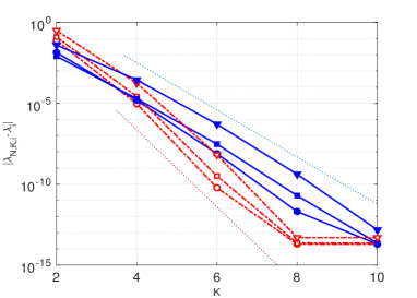
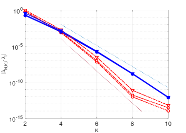
Figure 4.1. Approximation errors $|\lambda_{N,K,i}-\lambda_{i}|$ for (4.1) with $\mu=1/2$ versus $K$ by the MBPs spectral method using basis $S_{k,\ell,n,c}^{-1,\mu,1-\mu}(\bm{x})$ (primitive markers with dotted line) and $S_{k,\ell,n,c}^{-1,\mu,(1-\mu)/2}(\bm{x})$ (filled markers with full line) on the unit disk. $\circ:\lambda_{1}(n=0);\square:\lambda_{2}(n=1);\vartriangle:\lambda_{3}(n=2)$.( Left: $c=2$. Right: $c=10$).

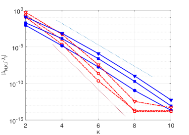
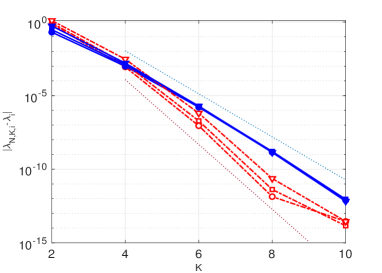
Figure 4.2. Approximation errors $|\lambda_{N,K,i}-\lambda_{i}|$ for (4.1) with $\mu=1/2$ versus $K$ by the MBPs spectral method using basis $S_{k,\ell,n,c}^{-1,\mu,1-\mu}(\bm{x})$ (primitive markers with dotted line) and $S_{k,\ell,n,c}^{-1,\mu,(1-\mu)/2}(\bm{x})$ (filled markers with full line) on the unit ball. $\circ:\lambda_{1}(n=0);\square:\lambda_{2}(n=1);\vartriangle:\lambda_{3}(n=2)$.( Left: $c=2$. Right: $c=10$).

Table 4.3. Radial normalized eigenfunctions of (4.1) with $n=0$, $\ell=1$, $\mu=1/2$ in $d=2$

$r$	$c$	Exact	Numerical
0.1	1	0.027609083125293	0.027609083125293
0.5	1	0.024094590264357	0.024094590264357
0.8	1	0.008294196243488	0.008294196243488
0.1	2	0.019361071632968	0.019361071632964
0.5	2	0.027859282291842	0.027859282291843
0.8	2	0.010413071837381	0.010413071837381

In Tables 4.1- 4.2, we tabulate the numerical eigenvalues for $\mu=1/2$ obtained by the MBP spectral method and the analytical values of the eigenvalues obtained by the analytical expression (4.2) for various choices of $c$, $n$, $k$ in $d=2$, and $d=3$, respectively. It is seen that our method is spectrally accurate. The approximations errors for the first third eigenvalues of the MBP spectral method with basis $S_{k,\ell,n,c}^{-1,\mu,1-\mu}(\bm{x})$ and $S_{k,\ell,n,c}^{-1,\mu,(1-\mu)/2}(\bm{x})$ are plotted in Figure 4.1 in simi-log scale for both $c=2$ and $c=10$ in $d=2$ dimensions for (4.1) with $\mu=1/2$, while in Figure 4.2, we give the approximation errors for the first third eigenvalues in simi-log scale for both $c=2$ and $c=10$ in $d=3$ dimensions for (4.1) with $\mu=1/2$. We see that the two MBP spectral methods share the spectral accuracy.

In Table 4.3, we list the values of the normalized eigenfunction in radial direction corresponding to the eigenvalues for several values of $r$ with $\mu=1/2$ in $d=2$. One can observe that numerical result obtained by the MBP spectral method match well with the expression (4.3). We denote by $\{u_{k,\ell}^{\mu,n}(\bm{x})\}$ as the normalized eigenfunction of (4.1). In Figures 4.3 and 4.4, we depict the surfaces and contours of $\{u_{k,\ell}^{\mu,n}(\bm{x},c)\}$ with different $c$, $k$, $\ell$, $n$ and $\mu=1/2$ in $d=2$. In Figures 4.5 and 4.6, we intend to visualize $\{u_{k,\ell}^{\mu,n}(\bm{x})\}$ with different $c$, $k$, $\ell$, $n$ and $\mu=0$ in $d=3$.

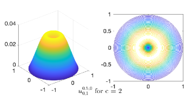
(a) $(\mu,n,k,\ell)=(0.5,0,0,1)$

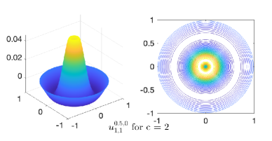
(b) $(\mu,n,k,\ell)=(0.5,0,1,1)$

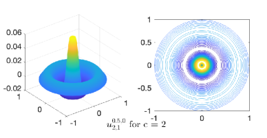
(c) $(\mu,n,k,\ell)=(0.5,0,2,1)$

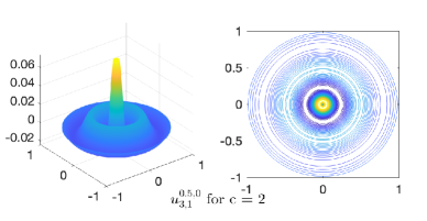
(d) $(\mu,n,k,\ell)=(0.5,0,3,1)$

Figure 4.3. Normalized eigenfunctions $\{u_{k,\ell}^{\mu,n}(\bm{x},c)\}$ with $c=2$, $\mu=1/2$ in $d=2$

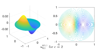
(a) $(\mu,n,k,\ell)=(0.5,1,0,1)$

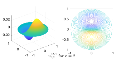
(b) $(\mu,n,k,\ell)=(0.5,1,0,2)$

(c) $(\mu,n,k,\ell)=(0.5,2,0,1)$

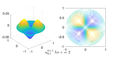
(d) $(\mu,n,k,\ell)=(0.5,2,0,2)$

Figure 4.4. Normalized eigenfunctions $\{u_{k,\ell}^{\mu,n}(\bm{x},c)\}$ with $c=2$, $\mu=1/2$ in $d=2$

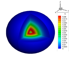
(a) $(\mu,n,k,\ell)=(0.5,0,0,1)$

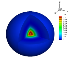
(b) $(\mu,n,k,\ell)=(0.5,0,1,1)$

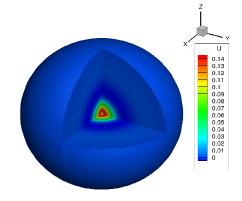
(c) $(\mu,n,k,\ell)=(0.5,0,2,1)$

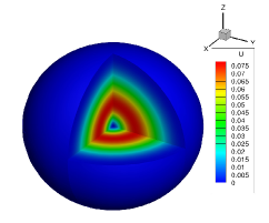
(d) $(\mu,n,k,\ell)=(0.5,2,0,1)$

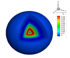
(e) $(\mu,n,k,\ell)=(0.5,2,1,1)$

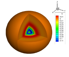
(f) $(\mu,n,k,\ell)=(0.5,2,2,1)$

Figure 4.5. Eigenfunctions $\{u_{k,\ell}^{\mu,n}(\bm{x},c)\}$ with $c=2$, $\mu=1/2$ in $d=3$

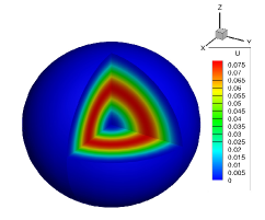
(a) $(\mu,n,k,\ell)=(0,0,0,1)$

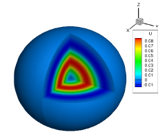
(b) $(\mu,n,k,\ell)=(0,0,1,1)$

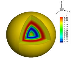
(c) $(\mu,n,k,\ell)=(0,0,2,1)$

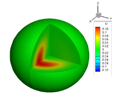
(d) $(\mu,n,k,\ell)=(0,1,0,2)$

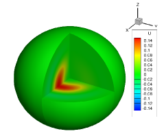
(e) $(\mu,n,k,\ell)=(0,1,1,2)$

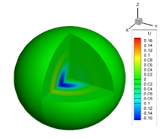
(f) $(\mu,n,k,\ell)=(0,1,2,2)$

Figure 4.6. Eigenfunctions $\{u_{k,\ell}^{\mu,n}(\bm{x},c)\}$ with $c=10$, $\mu=0$ in $d=3$

4.2. Schrödinger eigenvalue problems with fractional power potential

In the sequel, we consider the following Schrödinger equation with an inverse and a fractional power potential as follows

$$\left\{\begin{array}[]{ll}\Big{[}-\Delta+\displaystyle\frac{c}{\|\bm{x}\|^{2}}\Big{]}u(\bm{x})+z\|\bm{x}\|^{\frac{2\nu-2\eta}{\eta+1}}u(\bm{x})=\lambda u(\bm{x}),&\quad\bm{x}\in\mathbb{B}^{d},\\[4.0pt] u(\bm{x})=0,&\quad\bm{x}\in\mathbb{S}^{d-1},\end{array}\right.$$ (4.7)

where $\eta,\nu\in\mathbb{N}_{0}$. For any given rational number $\frac{q}{p}>-2$ with $p\in\mathbb{N}$ and $q\in\mathbb{Z}$, we can always rewrite it as

$$\frac{q}{p}=\frac{2\nu-2\eta}{\eta+1}\quad\text{ with }\quad\eta=2p-1\in\mathbb{N}_{0},\quad\nu=2p+q-1\in\mathbb{N}_{0}.$$

Note that the left-hand side of (4.1) in the spherical-polar coordinates can be reformulated as

$$-\Big{(}\partial^{2}_{r}+\frac{d-1}{r}\partial_{r}+\frac{\Delta_{0}-c}{r^{2}}\Big{)}u+zr^{\frac{2\nu-2\eta}{\eta+1}}u=-\frac{1}{r^{d-1}}\partial_{r}[r^{d-1}\partial_{r}]u-\frac{\Delta_{0}-c}{r^{2}}u+zr^{\frac{2\nu-2\eta}{\eta+1}}u.$$

Thus in the radial direction, we have

$$-\frac{1}{r^{d-1}}\partial_{r}(r^{d-1}\partial_{r}u_{\ell}^{n})+\frac{n(n+d-2)+c}{r^{2}}u_{\ell}^{n}+zr^{\frac{2\nu-2\eta}{\eta+1}}u_{\ell}^{n}$$ (4.8)

$$= -\Big{(}\partial_{r}^{2}u_{\ell}^{n}+\frac{d-1}{r}\partial_{r}u_{\ell}^{n}-\frac{n(n+d-2)+c}{r^{2}}u_{\ell}^{n}\Big{)}+zr^{\frac{2\nu-2\eta}{\eta+1}}u_{\ell}^{n}$$

$$= -\frac{1}{r^{\frac{d}{2}+\theta\beta_{n}}}\partial_{r}[r^{2\theta\beta_{n}+1}\partial_{r}(r^{\frac{d}{2}-\theta\beta_{n}-1}u_{\ell}^{n})]+zr^{\frac{2\nu-2\eta}{\eta+1}}u_{\ell}^{n}.$$

Using the variable substitution $\rho=r^{2\theta}$, we can write

$$-\frac{1}{r^{d-1}}\partial_{r}(r^{d-1}\partial_{r}u_{\ell}^{n})+\frac{n(n+d-2)+c}{r^{2}}u_{\ell}^{n}+zr^{\frac{2\nu-2\eta}{\eta+1}}u_{\ell}^{n}$$ (4.9)

$$= -\frac{4\theta^{2}}{r^{\frac{d}{2}+\theta\beta_{n}-2\theta+1}}\partial_{\rho}\big{[}\rho^{\beta_{n}+1}\partial_{\rho}\big{(}r^{\frac{d}{2}-\theta\beta_{n}-1}u_{\ell}^{n}\big{)}\big{]}+zr^{\frac{2\nu-2\eta}{\eta+1}}u_{\ell}^{n}.$$

If we take $\theta=\frac{1}{\eta+1}$, then the last term of (4.9) becomes $z\rho^{q}u_{\ell}^{n}$, so we choose the MBP approximation with $\alpha=-1$, $\mu=0$, $\theta=\frac{1}{\eta+1}$ to account for both the accuracy and efficiency. Accordingly, we introduce the approximation space

$$\mathcal{W}_{N,K}=\operatorname{span}\big{\{}S_{k,\ell,n,c}^{-1,0,\theta}(\bm{x}),\,(\ell,n)\in\Upsilon_{N}^{d},\,1\leq k\leq K,\,k\in\mathbb{N}_{0}\big{\}},\quad\theta=\frac{1}{\eta+1}.$$ (4.10)

Then the spectral scheme for (4.7) is to find $\lambda_{N,K}\in\mathbb{R}$ and $u_{N,K}\in\mathcal{W}_{\!N,K}\backslash\{0\}$, such that

$$\mathcal{B}(u_{N,K},v_{N,K})=\lambda_{N,K}(u_{N,K},v_{N,K}),\quad\forall\,v_{N,K}\in\mathcal{W}_{\!N,K},$$ (4.11)

where

$$\mathcal{B}(u_{N,K},v_{N,K})=(\nabla u_{N,K},\nabla v_{N,K})+c(\|\bm{x}\|^{-2}u_{N,K},v_{N,K})+z(\|\bm{x}\|^{\frac{2\nu-2\eta}{\eta+1}}u_{N,K},v_{N,K}).$$

In implementation, we write

$$u_{N,K}(\bm{x})=\sum_{n=0}^{N}\sum_{\ell=1}^{a_{n}^{d}}\sum_{k=1}^{K}\hat{u}_{k,\ell}^{n}S_{k,\ell,n,c}^{-1,0,\theta}(\bm{x}),$$

and denote

$$\begin{array}[]{l}\bm{u}=\big{(}\hat{\bm{u}}_{1}^{0},\hat{\bm{u}}_{2}^{0},\cdots,\hat{\bm{u}}_{a_{0}^{d}}^{0},\cdots,\hat{\bm{u}}_{1}^{N},\hat{\bm{u}}_{2}^{N},\cdots,\hat{\bm{u}}_{a_{N}^{d}}^{N}\big{)}^{t},\quad\hat{\bm{u}}_{\ell}^{n}=\big{(}\hat{u}_{1,\ell}^{n},\hat{u}_{2,\ell}^{n},\ldots,\hat{u}^{n}_{K,\ell}\big{)}^{t}.\end{array}$$

Corresponding to this ordering, we denote the stiffness and mass matrices by $\bm{S}$ and $\bm{M}$, respectively. The algebraic eigen-system of (4.11) reads

$$\bm{S}\bm{u}=\lambda_{N}\bm{M}\bm{u}.$$

Moreover, we can explicitly evaluate their entries. For fixed $k,j\in\mathbb{N}_{0}$, $(\ell,n),(\iota,m)\in\Upsilon_{\infty}^{d}$, we derive from (3.4) that

$$\begin{split}&\big{(}S_{k,\ell,n,c}^{-1,0,\theta},S_{j,\iota,m,c}^{-1,0,\theta}\big{)}=\int_{\mathbb{S}^{d-1}}Y_{\ell}^{n}(\bm{\hat{x}})Y_{\iota}^{m}(\bm{\hat{x}})\mathrm{d}\sigma(\bm{\hat{x}})\\ &\quad\times\int_{0}^{1}P_{k}^{(-1,\beta_{n})}(2r^{\frac{2}{\eta+1}}-1)P_{j}^{(-1,\beta_{n})}(2r^{\frac{2}{\eta+1}}-1)r^{\frac{2\beta_{n}}{\eta+1}+1}\mathrm{d}r\\ &=\delta_{kj}\delta_{nm}\int_{0}^{1}P_{k}^{(-1,\beta_{n})}(2r^{\frac{2}{\eta+1}}-1)P_{j}^{(-1,\beta_{n})}(2r^{\frac{2}{\eta+1}}-1)r^{\frac{2\beta_{n}}{\eta+1}+1}\mathrm{d}r\\ &=\delta_{kj}\delta_{nm}\displaystyle\frac{\eta+1}{2^{\beta_{n}+\eta+2}}\int_{-1}^{1}P_{k}^{(-1,\beta_{n})}(\rho)P_{j}^{(-1,\beta_{n})}(\rho)(\rho+1)^{\beta_{n}+\eta}\mathrm{d}\rho\qquad(\text{note: }\rho=2r^{2\theta}-1)\\ &=\delta_{kj}\delta_{nm}\displaystyle\frac{\eta+1}{2^{\beta_{n}+\eta+4}}\displaystyle\frac{k+\beta_{n}}{k}\displaystyle\frac{j+\beta_{n}}{j}\int_{-1}^{1}P_{k}^{(1,\beta_{n})}(\rho)P_{j}^{(1,\beta_{n})}(\rho)(1-\rho)^{2}(1+\rho)^{\beta_{n}+\eta}\mathrm{d}\rho,\end{split}$$

and

$$\big{(}{\|\bm{x}\|^{\frac{2\nu-2\eta}{\eta+1}}}S_{k,\ell,n,c}^{-1,0,\theta},S_{j,\iota,m,c}^{-1,0,\theta}\big{)}=\int_{\mathbb{S}^{d-1}}Y_{\ell}^{n}(\bm{\hat{x}})Y_{\iota}^{m}(\bm{\hat{x}})\mathrm{d}\sigma(\bm{\hat{x}})$$

$$\quad\times\int_{0}^{1}P_{k}^{(-1,\beta_{n})}(2r^{\frac{2}{\eta+1}}-1)P_{j}^{(-1,\beta_{m})}(2r^{\frac{2}{\eta+1}}-1)r^{\frac{2\beta_{n}+2\nu-2\eta}{\eta+1}+1}\mathrm{d}r$$

$$=\delta_{kj}\delta_{nm}\int_{0}^{1}P_{k}^{(-1,\beta_{n})}(2r^{\frac{2}{\eta+1}}-1)P_{j}^{(-1,\beta_{n})}(2r^{\frac{2}{\eta+1}}-1)r^{\frac{2\beta_{n}+2\nu-2\eta}{\eta+1}+1}\mathrm{d}r$$

$$=\delta_{kj}\delta_{nm}\displaystyle\frac{\eta+1}{2^{\beta_{n}+\nu+2}}\int_{-1}^{1}P_{k}^{(-1,\beta_{n})}(\rho)P_{j}^{(-1,\beta_{n})}(\rho)(\rho+1)^{\beta_{n}+\nu}\mathrm{d}\rho$$

$$=\delta_{kj}\delta_{nm}\displaystyle\frac{\eta+1}{2^{\beta_{n}+\nu+4}}\displaystyle\frac{k+\beta_{n}}{k}\displaystyle\frac{j+\beta_{n}}{j}\int_{-1}^{1}P_{k}^{(1,\beta_{n})}(\rho)P_{j}^{(1,\beta_{n})}(\rho)(1-\rho)^{2}(1+\rho)^{\beta_{n}+\nu}\mathrm{d}\rho.$$

Using Lemma 3.1 and (C.2), we find that the stiffness matrix $\bm{S}$ is a banded matrix with a bandwidth $2\nu+1$ and the mass matrix $\bm{M}$ is also banded with a bandwidth $2\eta+1$.

In the numerical tests, we fix $N=10$, and choose different values of $c,z,\eta,\nu,d$. in Figure 4.7, we depict the numerical errors between the first several eigenvalues by MBP spectral methods and the reference eigenvalues (obtained by the scheme with large $N$ and $K$). Exponential orders of convergence are clearly observed in all cases, which demonstrate the effectiveness of the MBP spectral method.

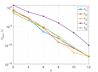
(a) $d=1,\eta=3,\nu=2,c=2,z=-3$

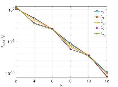
(b) $d=2,\eta=1,\nu=4,c=5,z=3$

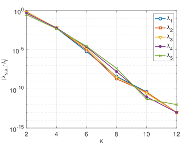
(c) $d=3,\eta=1,\nu=2,c=10,z=1$

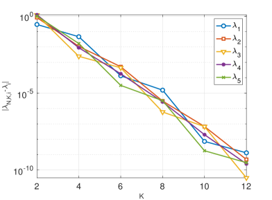
(d) $d=4,\eta=3,\nu=5,c=0.1,z=1$

Figure 4.7. The errors of the smallest $5$ eigenvalues versus $K$ for solving (4.7) with $N=10$

5. Concluding remarks

In this paper, we introduced a new family of orthogonal Müntz ball polynomials and presented various appealing properties. We then developed efficient and accurate MBP spectral-Galerkin methods for a class of degenerating eigenvalue problems with singular potentials and Schrödinger eigenvalue problems with fractional power potentials. The proposed approximation tools should have a much wider capability for numerical solutions of singular PDEs.

Declarations

• Availability of data and materials: The datasets generated during and/or analysed during the current study are available from the corresponding author on reasonable request.

• Authors’ contributions: All authors contributed to this study. The computations and the first draft were prepared by the first author. All authors read and approved the final manuscript.

• Conflict of interest statement: We have no conflicts of interest to disclose.

Appendix A Proof of Lemma 3.1

First, for the Laplace-Beltrami operator $\Delta_{0}$, it holds that (cf.​ [7, pp. 16, 26])

$$\quad\left(\nabla_{\!0}u,\nabla_{\!0}v\right)_{\mathbb{S}^{d-1}}=-\left(\Delta_{0}u,v\right)_{\mathbb{S}^{d-1}},\quad u\in H^{2}\left(\mathbb{S}^{d-1}\right),v\in H^{1}\left(\mathbb{S}^{d-1}\right).$$ (A.1)

We next prove that

$$\int_{0}^{1}\big{(}r^{d/2-\theta\beta_{n}-1+\mu}u\big{)}^{\prime}\big{(}r^{d/2-\theta\beta_{n}-1+\mu}v\big{)}^{\prime}r^{2\theta\beta_{n}+1}\mathrm{d}r$$

$$=\displaystyle\int_{0}^{1}\Big{[}r^{2\mu+d-1}u^{\prime}v^{\prime}+\Big{(}(\theta\beta_{n})^{2}-\big{(}\frac{d}{2}-(1-\mu)\big{)}^{2}\Big{)}r^{2\mu+d-3}uv\Big{]}\mathrm{d}r$$

$$\quad+\big{(}d/2-\theta\beta_{n}-1+\mu)\big{)}\big{(}u(1)v(1)-\delta_{2\mu+d,2}u(0)v(0)\big{)}.$$

We derive from direct calculation and integration by parts that

$$\displaystyle\int_{0}^{1}\big{(}r^{d/2-\theta\beta_{n}-1+\mu}u\big{)}^{\prime}\big{(}r^{d/2-\theta\beta_{n}-1+\mu}v\big{)}^{\prime}r^{2\theta\beta_{n}+1}\mathrm{d}r$$

$$=\displaystyle\int_{0}^{1}\Big{[}r^{2\mu+d-1}u^{\prime}v^{\prime}+r^{2\mu+d-3}\big{(}d/2-\theta\beta_{n}-1+\mu\big{)}^{2}uv$$

$$+\big{(}d/2-\theta\beta_{n}-1+\mu\big{)}r^{2\mu+d-2}(uv)^{\prime}\Big{]}\mathrm{d}r$$

$$=\displaystyle\int_{0}^{1}\Big{[}r^{2\mu+d-1}u^{\prime}v^{\prime}+r^{2\mu+d-3}\big{(}d/2-\theta\beta_{n}-1+\mu\big{)}^{2}uv$$ (A.2)

$$-(2\mu+d-2)\big{(}d/2-\theta\beta_{n}-1+\mu)\big{)}r^{2\mu+d-3}uv\Big{]}\mathrm{d}r$$

$$\quad+\big{(}d/2-\theta\beta_{n}-1+\mu)\big{)}\left[u(1)v(1)-0^{2\mu+d-2}u(0)v(0)\right]$$

$$\hskip 50.0pt=\displaystyle\int_{0}^{1}\Big{[}r^{2\mu+d-1}u^{\prime}v^{\prime}+\Big{(}(\theta\beta_{n})^{2}-\big{(}\frac{d}{2}-(1-\mu)\big{)}^{2}\Big{)}r^{2\mu+d-3}uv\Big{]}\mathrm{d}r$$

$$\quad+\big{(}d/2-\theta\beta_{n}-1+\mu)\big{)}\big{(}u(1)v(1)-\delta_{2\mu+d,2}u(0)v(0)\big{)}.$$

From (2.15), we know that

$$\bm{\hat{x}}\cdot\nabla_{0}=\bm{x}\cdot\nabla-r\partial_{r}=r\bm{\hat{x}}\cdot\nabla-r\partial_{r}=0,$$

so

$$\quad(\nabla u,\nabla v)_{\Omega}=\left(\nabla_{0}u,\nabla_{0}v\right)_{r^{-2},\Omega}+\left(\partial_{r}u,\partial_{r}v\right)_{\Omega},\quad\forall\,u,v\in H^{1}(\Omega).$$ (A.3)

Then from (A.1), (A.3) and (2.17), we obtain that

$$\big{(}\nabla\mathcal{S}_{k,\ell,n,c}^{-1,\mu,\theta},\nabla\mathcal{S}_{j,\iota,m,c}^{-1,\mu,\theta}\big{)}_{r^{2\mu}}+c\big{(}\mathcal{S}_{k,\ell,n,c}^{-1,\mu,\theta},\nabla\mathcal{S}_{j,\iota,m,c}^{-1,\mu,\theta}\big{)}_{r^{2\mu-2}}$$

$$=\big{(}\partial_{r}\mathcal{S}_{k,\ell,n,c}^{-1,\mu,\theta},\partial_{r}\mathcal{S}_{j,\iota,m,c}^{-1,\mu,\theta}\big{)}_{r^{2\mu}}+\big{(}\nabla_{\!0}\mathcal{S}_{k,\ell,n,c}^{-1,\mu,\theta},\nabla_{\!0}\mathcal{S}_{j,\iota,m,c}^{-1,\mu,\theta}\big{)}_{r^{2\mu-2}}+c\big{(}\mathcal{S}_{k,\ell,n,c}^{-1,\mu,\theta},\mathcal{S}_{j,\iota,m,c}^{-1,\mu,\theta}\big{)}_{r^{2\mu-2}}$$

$$=\big{(}\partial_{r}\mathcal{S}_{k,\ell,n,c}^{-1,\mu,\theta},\partial_{r}\mathcal{S}_{j,\iota,m,c}^{-1,\mu,\theta}\big{)}_{r^{2\mu}}-\big{(}\Delta_{0}\mathcal{S}_{k,\ell,n,c}^{-1,\mu,\theta},\mathcal{S}_{j,\iota,m,c}^{-1,\mu,\theta}\big{)}_{r^{2\mu-2}}+c\big{(}\mathcal{S}_{k,\ell,n,c}^{-1,\mu,\theta},\mathcal{S}_{j,\iota,m,c}^{-1,\mu,\theta}\big{)}_{r^{2\mu-2}}$$

$$=\big{(}\partial_{r}\mathcal{S}_{k,\ell,n,c}^{-1,\mu,\theta},\partial_{r}\mathcal{S}_{j,\iota,m,c}^{-1,\mu,\theta}\big{)}_{r^{2\mu}}+\left(c+n(n+d-2)\right)\big{(}\mathcal{S}_{k,\ell,n,c}^{-1,\mu,\theta},\mathcal{S}_{j,\iota,m,c}^{-1,\mu,\theta}\big{)}_{r^{2\mu-2}}.$$

For notational convenience, denote

$$q_{k,n}(r)=r^{\theta\beta_{n}+1-d/2-\mu}P_{k}^{(-1,\beta_{n})}(2r^{2\theta}-1).$$

We further obtain from (A) that

$$\big{(}\nabla\mathcal{S}_{k,\ell,n,c}^{-1,\mu,\theta},\nabla\mathcal{S}_{j,\iota,m,c}^{-1,\mu,\theta}\big{)}_{r^{2\mu}}+c\big{(}\mathcal{S}_{k,\ell,n,c}^{-1,\mu,\theta},\nabla\mathcal{S}_{j,\iota,m,c}^{-1,\mu,\theta}\big{)}_{r^{2\mu-2}}$$

$$=\int_{\mathbb{S}^{d-1}}Y_{\ell}^{n}(\bm{\hat{x}})Y_{\iota}^{m}(\bm{\hat{x}})d\sigma(\bm{\hat{x}})\int_{0}^{1}\left[r^{2\mu+d-1}q_{k,n}^{\prime}q_{j,n}^{\prime}+\left(c+n(n+d-2)\right)r^{2\mu+d-3}q_{k,n}q_{j,n}\right]\mathrm{d}r$$

$$=\delta_{nm}\delta_{\ell\iota}\int_{0}^{1}\big{(}r^{d/2-\theta\beta_{n}-1+\mu}q_{k,n}\big{)}^{\prime}\big{(}r^{d/2-\theta\beta_{n}-1+\mu}q_{j,n}\big{)}^{\prime}r^{2\theta\beta_{n}+1}\mathrm{d}r$$

$$\quad+\delta_{nm}\delta_{\ell\iota}\big{(}\theta\beta_{n}+1-d/2-\mu\big{)}\big{[}q_{k,n}(1)q_{j,n}(1)-\delta_{2\mu+d,2}\,q_{k,n}(0)q_{j,n}(0)\big{]}$$

$$=\delta_{nm}\delta_{\ell\iota}\int_{0}^{1}\big{(}P_{k}^{(-1,\beta_{n})}(2r^{2\theta}-1)\big{)}^{\prime}\big{(}P_{j}^{(-1,\beta_{n})}(2r^{2\theta}-1)\big{)}^{\prime}r^{2\theta\beta_{n}+1}\mathrm{d}r$$

$$\quad+\delta_{nm}\delta_{\ell\iota}\big{(}\theta\beta_{n}+1-d/2-\mu\big{)}\left[\delta_{k0}\delta_{kj}-\delta_{2\mu+d,2}\delta_{\theta\beta_{n}+1-d/2-\mu,0}\right]$$

$$=\delta_{nm}\delta_{\ell\iota}\frac{2\theta}{2^{\beta_{n}}}\int_{-1}^{1}\frac{\rm d}{{\rm d}{\rho}}P_{k}^{(-1,\beta_{n})}(\rho)\frac{\rm d}{{\rm d}{\rho}}P_{j}^{(-1,\beta_{n})}(\rho)(1+\rho)^{\beta_{n}+1}\mathrm{d}\rho$$

$$\quad+\delta_{nm}\delta_{\ell\iota}\big{(}\theta\beta_{n}+1-d/2-\mu\big{)}\delta_{k0}\delta_{kj},$$

where in the last equatlity, we use the variable transformation $\rho=r^{2\theta}-1$. Using the property

$$\frac{\rm d}{{\rm d}x}P_{k}^{(-1,\beta_{n})}(x)=\frac{k+\beta_{n}}{2}P_{k-1}^{(0,\beta_{n}+1)}(x),$$ (A.4)

We derive from (A.4) and (2.1) that

$$\int_{-1}^{1}\frac{\rm d}{{\rm d}{\rho}}P_{k}^{(-1,\beta_{n})}(\rho)\frac{\rm d}{{\rm d}{\rho}}P_{j}^{(-1,\beta_{n})}(\rho)(1+\rho)^{\beta_{n}+1}\mathrm{d}\rho$$

$$= \frac{(k+\beta_{n})(j+\beta_{n})}{4}\int_{-1}^{1}P_{k-1}^{(0,\beta_{n}+1)}(\rho)P_{j-1}^{(0,\beta_{n}+1)}(\rho)(1+\rho)^{\beta_{n}+1}\mathrm{d}\rho$$

$$= \frac{2^{\beta_{n}}(k+\beta_{n})^{2}}{2k+\beta_{n}}\delta_{kj}.$$ (A.5)

This completes the proof.

Appendix B Proof of Proposition 4.1

Using the Leibniz rule for gradient and divergence, we can reformulate the problem in the spherical-polar coordinates as follows:

$$-r^{2\mu}\Big{(}\partial^{2}_{r}+\frac{2\mu+d-1}{r}\partial_{r}+\frac{\Delta_{0}-c}{r^{2}}\Big{)}u=-\frac{1}{r^{d-1}}\partial_{r}(r^{2\mu+d-1}\partial_{r}u)-\frac{\Delta_{0}-c}{r^{2-2\mu}}u=\lambda u.$$

We now represent the unknown eigenfunction $u$ as an expansion of spherical harmonic function,

$$u(\bm{x})=\sum_{n=0}^{\infty}\sum_{\ell=1}^{a_{n}^{d}}u_{\ell}^{n}(r)Y_{\ell}^{n}(\bm{\hat{x}}),$$

and then obtain the radial eigenvalue problem

$$-\frac{1}{r^{d-1}}\partial_{r}\big{(}r^{2\mu+d-1}\partial_{r}u_{\ell}^{n}(r)\big{)}+\frac{n(n+d-2)+c}{r^{2-2\mu}}u_{\ell}^{n}(r)=\lambda u_{\ell}^{n}(r),\quad 1\leq\ell\leq a_{n}^{d},\;\;n\geq 0.$$ (B.1)

Let $r=\rho^{\frac{1}{1-\mu}}$ and set $v_{\ell}^{n}(\rho)=u_{\ell}^{n}(r)$. We can reformulate (B.1) as

$$-\frac{1}{\rho^{\frac{d}{1-\mu}-1}}\partial_{\rho}\big{[}\rho^{\frac{d}{1-\mu}-1}\partial_{\rho}v_{\ell}^{n}(\rho)\big{]}+\frac{n(n+d-2)+c}{(1-\mu)^{2}\rho^{2}}v_{\ell}^{n}(\rho)=\frac{\lambda}{(1-\mu)^{2}}v_{\ell}^{n}(\rho),$$ (B.2)

and (B.1) can be written as

$$\rho^{2}\partial_{\rho}^{2}\big{[}\rho^{\frac{d}{2(1-\mu)}-1}v_{\ell}^{n}(\rho)\big{]}+\rho\partial_{\rho}\big{[}\rho^{\frac{d}{2(1-\mu)}-1}v_{\ell}^{n}(\rho)\big{]}+\big{[}\frac{\lambda}{(1-\mu)^{2}}\rho^{2}-\frac{\beta_{n}^{2}}{4}\big{]}\rho^{\frac{d}{2(1-\mu)}-1}v_{\ell}^{n}(\rho)=0.$$

Making the variable transformation $\eta=\frac{\sqrt{\lambda}}{1-\mu}\rho$ and setting $\chi_{\ell}^{n}(\eta)=\rho^{\frac{d}{2(1-\mu)}-1}v_{\ell}^{n}(\rho)$, one obtains

$$\eta^{2}\partial_{\eta}^{2}\chi_{\ell}^{n}(\eta)+\eta\partial_{\eta}\chi_{\ell}^{n}(\eta)+\Big{(}\eta^{2}-\frac{\beta_{n}^{2}}{4}\Big{)}\chi_{\ell}^{n}(\eta)=0,$$

which is exactly the Sturm-Liouville equation for the first kind Bessel function and here admits a unique solution $\chi_{\ell}^{n}(\eta)=J_{\frac{\beta_{n}}{2}}(\eta)$, where $J_{\alpha}(x)$ is the first kind Bessel function which can be expressed as

$$J_{\alpha}(x)=\sum_{m=0}^{\infty}\frac{(-1)^{m}}{m!\Gamma(m+\alpha+1)}\left(\frac{x}{2}\right)^{2m+\alpha}.$$

In return,

$$u_{\ell}^{n}(r) =v_{\ell}^{n}(\rho)=\rho^{1-\frac{d}{2(1-\mu)}}\chi_{n}(\eta)=\rho^{1-\frac{d}{2(1-\mu)}}J_{\frac{\beta_{n}}{2}}\Big{(}\frac{\sqrt{\lambda}}{1-\mu}\rho\Big{)}=r^{1-\mu-\frac{d}{2}}J_{\frac{\beta_{n}}{2}}\Big{(}\frac{\sqrt{\lambda}}{1-\mu}r^{1-\mu}\Big{)}$$ (B.3)

$$=\sum_{m=0}^{\infty}\frac{(-1)^{m}}{m!\Gamma\big{(}m+\frac{\beta_{n}}{2}+1\big{)}}\Big{(}\frac{\sqrt{\lambda}r^{1-\mu}}{2(1-\mu)}\Big{)}^{2m+\beta_{n}/2}r^{1-\mu-\frac{d}{2}}.$$

Since the homogeneous Dirichlet boundary condition implies $u_{\ell}^{n}(1)=0$, one readily finds that the eigenvalue $\lambda$ of (B.1) satisfies

$$J_{\frac{\beta_{n}}{2}}\Big{(}\frac{\sqrt{\lambda}}{1-\mu}\Big{)}=0.$$

This completes the derivation.

Appendix C Proof of Lemma 4.1

From (3.4), it is easy to see that

$$\big{(}S_{k,\ell,n,c}^{-1,\mu,1-\mu},S_{j,\iota,m,c}^{-1,\mu,1-\mu}\big{)}=\int_{\mathbb{S}^{d-1}}Y_{\ell}^{n}(\bm{\hat{x}})Y_{\iota}^{m}(\bm{\hat{x}})\mathrm{d}\sigma(\bm{\hat{x}})$$

$$\quad\times\int_{0}^{1}P_{k}^{(-1,\beta_{n})}(2r^{2-2\mu}-1)P_{j}^{(-1,\beta_{m})}(2r^{2-2\mu}-1)r^{(1-\mu)(\beta_{n}+\beta_{m})-2\mu+1}\mathrm{d}r$$

$$=\delta_{kj}\delta_{nm}\int_{0}^{1}P_{k}^{(-1,\beta_{n})}(2r^{2-2\mu}-1)P_{j}^{(-1,\beta_{n})}(2r^{2-2\mu}-1)r^{2(1-\mu)(\beta_{n}+1)-1}\mathrm{d}r$$

$$=\delta_{kj}\delta_{nm}\frac{1}{2^{2+\beta_{n}}(1-\mu)}\int_{-1}^{1}P_{k}^{(-1,\beta_{n})}(\rho)P_{j}^{(-1,\beta_{n})}(\rho)(1+\rho)^{\beta_{n}}\mathrm{d}\rho.$$ (C.1)

where in the last inequality, we use the change of variable $\rho=2r^{2-2\mu}-1$. Then, from the properties of Jacobi polynomials in (2.5) and (3.21), we obtain

$$P_{k}^{(\alpha,\beta)}(x)=\frac{k+\alpha+\beta+1}{2k+\alpha+\beta+1}P_{k}^{(\alpha+1,\beta)}(x)-\frac{k+\beta}{2k+\alpha+\beta+1}P_{k-1}^{(\alpha+1,\beta)}(x),$$ (C.2)

which implies

$$P_{k}^{(-1,\beta_{n})}=\frac{(k+\beta_{n})}{(2k+\beta_{n})}P_{k}^{(0,\beta_{n})}-\frac{(k+\beta_{n})}{(2k+\beta_{n})}P_{k-1}^{(0,\beta_{n})}.$$ (C.3)

Then a combination of (C), (C.3), and (2.1) immediately yields (4.6).

References

- [1] G. E. Andrews, R. Askey, and R. Roy, Special functions, vol. 71, Cambridge University Press, Cambridge, 1999.
- [2] K. Atkinson, D. Chien, and O. Hansen, Spectral Methods Using Multivariate Polynomials On The Unit Ball, CRC Press, 2019.
- [3] L. Cagliero and T. H. Koornwinder, Explicit matrix inverses for lower triangular matrices with entries involving Jacobi polynomials, J. Approx. Theory, 193 (2015), pp. 20–38.
- [4] D. Cao and P. Han, Solutions to critical elliptic equations with multi-singular inverse square potentials, J. Differential Equations, 224 (2006), pp. 332–372.
- [5] E. W. Cheney, Introduction to approximation theory, AMS Chelsea Publishing, Providence, RI, 1998. Reprint of the second (1982) edition.
- [6] T. S. Chihara, An introduction to orthogonal polynomials, vol. 13, Gordon and Breach Science Publishers, New York-London-Paris, 1978.
- [7] F. Dai and Y. Xu, Approximation theory and harmonic analysis on spheres and balls, Springer, New York, 2013.
- [8] C. F. Dunkl and Y. Xu, Orthogonal polynomials of several variables, vol. 155 of Encyclopedia of Mathematics and its Applications, Cambridge University Press, Cambridge, second ed., 2014.
- [9] B. o. Dyda, A. Kuznetsov, and M. Kwaśnicki, Eigenvalues of the fractional Laplace operator in the unit ball, J. Lond. Math. Soc. (2), 95 (2017), pp. 500–518.
- [10] , Fractional Laplace operator and Meijer G-function, Constr. Approx., 45 (2017), pp. 427–448.
- [11] V. Felli, E. M. Marchini, and S. Terracini, On Schrödinger operators with multipolar inverse-square potentials, J. Funct. Anal., 250 (2007), pp. 265–316.
- [12] V. Felli and S. Terracini, Elliptic equations with multi-singular inverse-square potentials and critical nonlinearity, Comm. Partial Differential Equations, 31 (2006), pp. 469–495.
- [13] A. Kufner, Weighted Sobolev spaces, A Wiley-Interscience Publication, John Wiley & Sons, Inc., New York, 1985. Translated from the Czech.
- [14] H. Li and J. Shen, Optimal error estimates in Jacobi-weighted Sobolev spaces for polynomial approximations on the triangle, Math. Comp., 79 (2010), pp. 1621–1646.
- [15] H. Li and Y. Xu, Spectral approximation on the unit ball, SIAM J. Numer. Anal., 52 (2014), pp. 2647–2675.
- [16] H. Li and Z. Zhang, Efficient spectral and spectral element methods for eigenvalue problems of Schrödinger equations with an inverse square potential, SIAM J. Sci. Comput., 39 (2017), pp. A114–A140.
- [17] S. Ma, H. Li, and Z. Zhang, Efficient spectral methods for some singular eigenvalue problems, J. Sci. Comput., 77 (2018), pp. 657–688.
- [18] S. Olver and Y. Xu, Orthogonal polynomials in and on a quadratic surface of revolution, Math. Comp., 89 (2020), pp. 2847–2865.
- [19] C. Sheng, S. Ma, H. Li, L.-L. Wang, and L. Jia, Nontensorial generalised Hermite spectral methods for PDEs with fractional Laplacian and Schrödinger operators, ESAIM Math. Model. Numer. Anal., 55 (2021), pp. 2141–2168.
- [20] G. Szegő, Orthogonal polynomials, vol. XXIII, American Mathematical Society, Providence, R.I., fourth ed., 1975.
- [21] J. Zhang, H. Li, L.-L. Wang, and Z. Zhang, Ball prolate spheroidal wave functions in arbitrary dimensions, Appl. Comput. Harmon. Anal., 48 (2020), pp. 539–569.