Smooth and Stepwise Self-Distillation for Object Detection

Abstract

Distilling the structured information captured in feature maps has contributed to improved results for object detection tasks, but requires careful selection of baseline architectures and substantial pre-training. Self-distillation addresses these limitations and has recently achieved state-of-the-art performance for object detection despite making several simplifying architectural assumptions. Building on this work, we propose Smooth and Stepwise Self-Distillation (sssd) for object detection. Our sssd architecture forms an implicit teacher from object labels and a feature pyramid network backbone to distill label-annotated feature maps using Jensen-Shannon distance, which is smoother than distillation losses used in prior work. We additionally add a distillation coefficient that is adaptively configured based on the learning rate. We extensively benchmark sssd against a baseline and two state-of-the-art object detector architectures on the COCO dataset by varying the coefficients and backbone and detector networks. We demonstrate that sssd achieves higher average precision in most experimental settings, is robust to a wide range of coefficients, and benefits from our stepwise distillation procedure.

Index Terms—  knowledge distillation, object detection, Jensen-Shannon distance, stepwise distillation

1 Introduction

Knowledge distillation is a technique for transferring the information contained in the feature maps and model outputs of a large teacher model to a typically smaller student model [1, 2]. As a result, student models have lower storage and memory requirements and yield more efficient inference, enabling use in limited resource or real-time settings like in edge devices or autonomous vehicles [3, 4]. Object detection is among the largest beneficiary of knowledge distillation [5, 6, 7] and transfer learning on related tasks [8], but these techniques require careful selection of a baseline teacher model and expensive pre-training [7, 9]. Recent work removes the dependency on a pre-trained teacher entirely, e.g. by collaboratively training a collection of student networks (collaborative learning) [10] or smoothing class labels (label regularization) [11, 12]; however, these methods have largely focused on image classification.

Unlike traditional transfer learning and knowledge distillation, self-distillation aims at extracting knowledge from the data labels during feature extraction within the same backbone model [5, 6, 7, 13, 14]; this eliminates the need for expensive pre-training of a teacher network. LabelEnc is a recently developed self-distillation method for object detection that encodes label information within the feature maps, providing intermediate supervision at internal neural network layers and achieving an approximately 2% improvement over prior work in the COCO dataset [14]. Building on LabelEnc, label-guided self-distillation (LGD) leverages both label- and feature map-encodings as knowledge and improved the benchmark set by LabelEnc on COCO [13].

While LabelEnc and LGD achieve state-of-the-art performance, they make simplifying architectural assumptions. First, they consider mean squared error (MSE) as the only distillation loss, which is not robust to the noisy or imperfect teachers that are commonplace in self-distillation settings [15]. Second, there is no consideration for how the knowledge distillation coefficient $\lambda$ affects the total loss or overall performance. In this paper, we explore the limitations of MSE as a self-distillation loss and the sensitivity of self-distillation to $\lambda$. We propose Smooth and Stepwise Self-Distillation (sssd) by combining the Jensen-Shannon (JS) divergence with a $\lambda$ that is adaptively configured based on the learning rate in a stepwise manner (Fig. 1). We summarize our contributions as follows:

• We present Smooth and Stepwise Self-Distillation (sssd), which combines stepwise self-distillation with a smooth, bounded, and symmetric distance that is robust to noise (JS) [16, 17, 18].

• We study the sensitivity of self-distillation to the distillation coefficient $\lambda$ under a variety of architectural assumptions, providing insight on how $\lambda$ influences model performance.

• We thoroughly benchmark sssd and demonstrate higher average precision than previous self-distillation approaches in most configurations of the backbone and detector networks.

Fig. 1: Smooth and Stepwise Self-Distillation (sssd). The feature maps ($\bm{K}$) extracted from the backbone (ResNet-50) are sent to the fusion component along with the ground truth annotations. The distillation loss ($L_{distill}$) is calculated using the feature maps and label enhanced feature maps ($\bm{K_{e}}$). The detection loss ($L_{det}$) is calculated as classification and bounding-box regression losses by a shared detection head.

2 Proposed Method

2.1 Smooth Self-Distillation

Leveraging prior work on self-distillation for object detection, the features are obtained from a backbone feature pyramid network with $P$ scales [14, 13]. We define $\bm{K}=\{\bm{k}^{p}\in\mathbb{R}^{N_{p}\times M_{p}}\}^{P}$ to be the set of features from the backbone feature pyramid network where $\bm{k}^{p}$ is a vector of features at the $p^{th}$ scale, each pyramid has dimension $N_{p}\times M_{p}$, and $p\in\{1,\dots,P\}$. Similarly, let $\bm{K}_{e}=\{\bm{k}^{p}_{e}\in\mathbb{R}^{N_{p}\times M_{p}}\}^{P}$ be the feature maps obtained from a spatial transformer network [19] (STN) by the label-annotated feature maps (denoted by $e$) in the fusion component (Fig. 1). Existing self-distillation methods for object detection use mean squared error (MSE) to calculate the distillation loss [13, 14]:

$$L^{MSE}_{distill}=\frac{1}{N}\sum^{P}_{p=1}||\bm{k}^{p}-\bm{k}^{p}_{e}||^{2},$$

where $N=\sum^{P}_{p=1}N_{p}\times M_{p}$ is the total number of feature map elements. The Kullback-Leibler (KL) divergence is another commonly used loss function that was used to initially define knowledge distillation [1] and used subsequently across many applications [20, 21, 22, 23]:

$$L^{KL}_{distill}=\frac{1}{N}\sum^{P}_{p=1}D_{KL}(\bm{k}^{p}||\bm{k}^{p}_{e}),$$

However, the KL divergence has several limitations. For probability distributions $O$ and $Q$, $D_{KL}(O||Q)$ is not bounded, which may result in model divergence during training, and is sensitive to regions of $O$ and $Q$ that have low probability; e.g., $D_{KL}(O||Q)$ can be large when $O(x)>>Q(x)$ for an event $x$ even if $O(x)$ is small when $Q(x)$ is close to $0$ [24]. To address these issues, we use the Jensen-Shannon (JS) divergence as a new measure for knowledge distillation in object detection tasks. Unlike KL divergence, the JS divergence is bounded by $[0,1]$, symmetric, does not require absolute continuity [25], and has been shown to be robust to label noise [16, 17, 18] and imperfect teachers that are commonplace in self-distillation settings [15]:

$$D_{JS}(O||Q) =D_{JS}(Q||O)$$

$$=\frac{1}{2}D_{KL}(O||M)+\frac{1}{2}D_{KL}(Q||M)$$

where $M=\frac{1}{2}(O+Q)$. In this work, we consider the JS distance, which is a metric defined by $(D_{JS}(O||Q))^{\frac{1}{2}}$. We define the distillation loss, $L_{distill}$, as:

$$L_{distill}=\frac{1}{N}\sum^{P}_{p=1}\left(D_{JS}(\bm{k}^{p}||\bm{k}^{p}_{e})\right)^{\frac{1}{2}},$$

The detection loss is defined as:

$$L_{det}=\hat{L}_{det}(H(\bm{K}),Y)+\hat{L}^{e}_{det}(H(\bm{K}_{e}),Y)$$

where the $H(\cdot)$ refers to the shared detection head, $Y$ is the ground truth, and $\hat{L}$ is a classification and regression object detection loss. Thereby, we obtain the total training objective as:

$$L_{total}=L_{det}+\lambda L_{distill}$$

where $\lambda$ is a coefficient for the distillation loss. Our choice of functional form for $L_{distill}$ was motivated by research suggesting smooth loss functions improve deep neural network training and performance [26, 27]; since the JS distance $D_{JS}(0||Q)$ is considered to be a smooth compromise between $D_{KL}(O||Q)$ and $D_{KL}(Q||O)$, we term this knowledge distillation method as smooth self-distillation.

2.2 Stepwise Self-Distillation

Learning rate scheduling is broadly used in large scale deep learning as an important mechanism to adjust the learning rate during training, typically through learning rate reduction according to a predefined schedule. To help the model continue learning from self-distillation during learning rate decay, we propose stepwise self-distillation to compensate for the lessened impact of the self-distillation loss caused by a reduced learning rate. In our setting, the backbone model is frozen and the detector is trained in the first 20$k$ iterations. An initial $\lambda$ is assigned to the distillation loss empirically after the first 20$k$ iterations; selection of an empirical $\lambda$ is elaborated in the experimental section. We redefine the $\lambda$ in stepwise self-distillation as a step function of $\lambda_{1}$ and a $\lambda_{2}$ that depends on the training iteration. Since in our model training the learning rate begins decaying at iteration $120,000$, we define $\lambda$ as:

$$\lambda=\begin{cases}\lambda_{1},\quad&steps<120000\\ \lambda_{2},\quad&steps\geq 120000\end{cases}$$

3 Experiments

We compared sssd with two state-of-the-art (SOTA) self-distillation architectures for object detection, LabelEnc [14] and LGD [13], and a non-distillation baseline model. All experiments were conducted using the official code repositories for LabelEnc [28] and LGD [29], using a batch size of $16$ on $8$ NVIDIA v100 GPUs and configurations specified in their official GitHub repositories. Our experiments tested different backbone networks, ResNet-50 (R-50) and ResNet-101 (R-101), and explored three popular detectors: Faster R-CNN (FRCN) [30], fully convolutional one-stage object detector (FCOS) [31] and RetinaNet [32]. All experiments were validated on the Microsoft Common Objects in Context (COCO) dataset with $80$ categories using commonly reported metrics based on mean average precision (AP) and other detailed metrics: APs, APm, and APl, which are the AP for small, medium and large objects, and AP50 and AP75, which are the AP at IoU=0.50 and IoU=0.75 where IoU is the intersection over union [33].

3.1 Comparisons with SOTA Results

We first compared sssd with competing methods on the COCO data based on AP and using two backbone networks, R-50 and R-101, and three detectors, FRCN, RetinaNet and FCOS (Table 1). Compared to the baseline model, our approach achieved an AP improvement of approximately $2.0\%$, $3.6\%$, and $3.2\%$ for the FRCN, RetinaNet, and FCOS detectors respectively. Our method improved on the AP of LabelEnc by approximately 2.8% for FRCN_R50, 2.2% for FRCN_R101, and more than 1% for other architectural configurations. With respect to LGD, sssd achieves an almost $1\%$ gain in AP for the FRCN_R50 and FCOS_R101 configurations and $<0.5\%$ improvements in other FRCN and FCOS settings.

Since the performance of LGD is most comparable to sssd, we further investigated the performance of LGD and sssd using variations of AP (Table 2). In the RetinaNet_R101 setting, our proposed method achieved a $5\%$ AP performance gain ($26.1$ versus $24.9$) for objects with small bounding boxes (APs). The results for the other detectors demonstrate that sssd performs relatively well compared with LGD primarily due to improved AP for objects with medium or large bounding boxes (APm and APl). FCOS_R101-based architectures yielded the best AP results for both methods where sssd outperformed LGD in all AP-related measures besides APs, including a $0.6\%$, $0.8\%$, and $1\%$ gain over LGD in AP50, APm, and APl respectively.

Table 1: Comparisons with baseline and SOTA methods based on mean average precision (AP).

Detector	Backbone	Baseline	LabelEnc	LGD	Ours
FRCN	R-50	39.6	39.6	40.4	40.6
	R-101	41.7	41.4	42.2	42.3
RetinaNet	R-50	38.8	39.6	40.3	40.2
	R-101	40.6	41.5	42.1	42.1
FCOS	R-50	41.0	41.8	42.3	42.4
	R-101	42.9	43.6	44.0	44.2

Table 2: Detailed Comparisons with LGD.

	AP	AP50	AP75	APs	APm	APl
FRCNR50-Ours	40.6	61.2	44.0	23.8	43.9	53.2
FRCNR50-LGD	40.4	61.3	43.9	24.0	43.9	52.2
FRCNR101-Ours	42.3	62.9	45.8	25.3	45.9	56.3
FRCNR101-LGD	42.2	62.8	45.5	25.9	45.5	56.0
RetinaNetR50-Ours	40.2	60.0	43.0	24.2	44.2	52.1
RetinaNetR50-LGD	40.3	60.1	43.0	24.0	44.1	52.4
RetinaNetR101-Ours	42.1	61.9	44.9	26.1	46.2	55.1
RetinaNetR101-LGD	42.1	62.1	45.1	24.9	46.5	55.0
FCOSR50-Ours	42.4	61.2	46.0	26.4	46.1	54.0
FCOSR50-LGD	42.4	61.2	45.8	26.2	46.1	54.3
FCOSR101-Ours	44.2	63.3	47.6	27.1	48.3	57.5
FCOSR101-LGD	44.0	62.9	47.5	27.2	47.9	56.9

3.2 Effect of Adjusting $\lambda$

Next, we considered the effect of varying the distillation coefficient, $\lambda$. While previous work assumed a $\lambda=1$ [13], we conjectured that adjusting $\lambda$ may be beneficial for model training due to varying the contribution of the distillation loss to the overall loss function during learning rate decay. Since we are using a different distillation loss than LGD, we first calibrated the $\lambda$ parameter between LGD and sssd. First, we reproduced the original experiments by setting $\lambda=1$ in LGD with the FRCN detector and R50 backbone; the mean contribution of the penalized distillation loss to the total loss ($\lambda L_{distill}/L_{total}$) was 45% after $1,000$ iterations. We computed a $\lambda$ in the domain of $[1,100]$ using binary search that yielded a mean $\lambda L_{distill}/L_{total}\approx 0.45$ after $1,000$ iterations, which led to an equivalent $\lambda$ of $50$ for sssd. To explore the impact of adjusting $\lambda$, we considered $\lambda\in\{1,1.5,2\}$ for LGD and $\lambda\in\{50,75,100\}$ for sssd. The $\lambda L_{distill}/L_{total}$ at iteration $17\times 10^{4}$ was similar across the two architectures (Table 3). Interestingly, the final $\lambda L_{distill}/L_{total}$ was close to $50\%$ for both LGD and sssd regardless of the $\lambda$.

We compared the performance between LGD and sssd after calibrating $\lambda L_{distill}/L_{total}$ to be in a comparable range (Fig. 2 and Table 4). The top performing $\lambda$ for sssd ($75$) consistently outperformed the top performing LGD configuration ($\lambda=1$) in all AP measures besides AP50; when considering all $\lambda$, sssd compares favorably to LGD among most of the AP variants, including up to a $1.1\%$ ($44.1$ versus $43.6$) improvement in AP75 (Table 4). The top performing sssd also maintains an advantage over LGD from iterations $13\times 10^{4}$ to $17\times 10^{4}$ (Fig. 2).

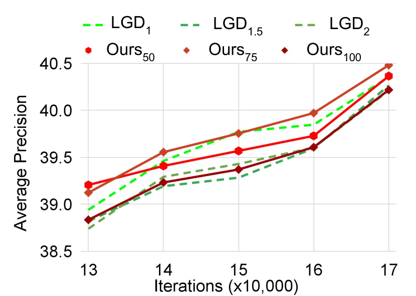
Fig. 2: Performance comparison with different $\lambda$. After calibrating the distillation loss, the AP for sssd with $\lambda=75$ (Ours₇₅) is higher than LGD configurations. The learning rates for each architecture are $0$ after iteration $17\times 10^{4}$.

Table 3: Comparisons of $\lambda L_{distill}/L_{total}$ with different $\lambda$ after iterations $17\times 10^{4}$.

LGD1	LGD1.5	LGD2	Ours50	Ours75	Ours100
0.44	0.46	0.58	0.41	0.49	0.47

Table 4: Detailed Comparisons with different $\lambda$ selections.

	AP	AP50	AP75	APs	APm	APl
LGD1	40.4	61.3	43.6	23.5	43.7	53.1
LGD1.5	40.2	60.8	43.3	23.8	43.3	52.7
LGD2	40.2	60.9	43.6	23.5	43.5	53.0
Ours50	40.5	61.2	44.1	23.8	43.5	53.2
Ours75	40.6	61.2	44.0	23.8	43.9	53.2
Ours100	40.2	60.7	43.4	23.5	43.4	52.6

3.3 Stepwise Distillation

Finally, we evaluated the effectiveness of stepwise distillation in both LGD and sssd using a fixed architecture (FRCN-R50) over the final $60,000$ iterations (Fig. 3). We tested LGD $\lambda_{1}=1$ and sssd $\lambda_{1}=75$ since these were the best performing $\lambda$ for this architecture (Table 4). Additionally, we tested a slightly increased LGD $\lambda_{2}=1.5$ and sssd $\lambda_{2}=80$. We compared these static $\lambda$ settings with stepwise distillation, which switches from $\lambda_{1}$ to $\lambda_{2}$ at iteration $120,000$ (in the learning rate scheduler period). Stepwise distillation improves both LGD and sssd resulting in an approximately $0.5\%$ improvement in AP over fixed $\lambda$ settings (Fig. 3). Since stepwise distillation does not impose additional computational costs and is independent of the architecture, we optimistically believe that stepwise distillation may be beneficial for other knowledge distillation applications.

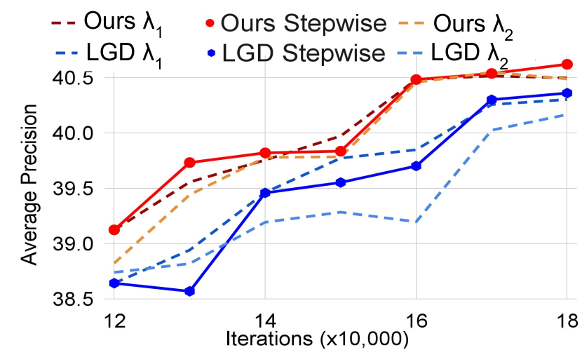
Fig. 3: Stepwise self-distillation comparisons. The stepwise self-distillation strategy for both LGD and sssd (Ours) improves final AP over a fixed $\lambda$.

4 Conclusion

In this paper, we proposed Smooth and Stepwise Self-Distillation (sssd) for object detection, which can efficiently improve model performance without requiring a large teacher model. Through extensive benchmarking, we demonstrated that sssd achieves improved performance when compared with current SOTA self-distillation approaches for a variety of backbones and detectors. We investigated the effects of varying the distillation coefficient and justified stepwise distillation as a potentially beneficial procedure for improving the performance of knowledge distillation schemes.

References

- [1] Geoffrey Hinton et al., “Distilling the Knowledge in a Neural Network,” 2015.
- [2] Cristian Bucilua et al., “Model Compression,” in SIGKDD, 2006.
- [3] Manoj Bharadhwaj et al., “Detecting Vehicles on the Edge: Knowledge Distillation To Improve Performance in Heterogeneous Road Traffic,” in CVPR, 2022.
- [4] Divya Kothandaraman et al., “Domain adaptive knowledge distillation for driving scene semantic segmentation,” in WACV, 2021.
- [5] Gang Li et al., “Knowledge Distillation for Object Detection via Rank Mimicking and Prediction-Guided Feature Imitation,” AAAI, 2022.
- [6] Zijian Kang et al., “Instance-Conditional Knowledge Distillation for Object Detection,” in NeurIPS. 2021, Curran Associates, Inc.
- [7] Linfeng Zhang and Kaisheng Ma, “Improve Object Detection with Feature-based Knowledge Distillation: Towards Accurate and Efficient Detectors,” in ICLR, 2021.
- [8] Cristina Vasconcelos et al., “Proper Reuse of Image Classification Features Improves Object Detection,” in CVPR, 2022.
- [9] Lewei Yao et al., “G-DetKD: Towards general distillation framework for object detectors via contrastive and semantic-guided feature imitation,” in ICCV, 2021.
- [10] Qiushan Guo et al., “Online knowledge distillation via collaborative learning,” in CVPR, 2020.
- [11] Rafael Müller et al., “When does label smoothing help?,” NeurIPS, 2019.
- [12] Qianggang Ding et al., “Adaptive regularization of labels,” arXiv, 2019.
- [13] Peizhen Zhang et al., “LGD: Label-guided Self-distillation for Object Detection,” in AAAI, 2022.
- [14] Miao Hao et al., “LabelEnc: A New Intermediate Supervision Method for Object Detection,” in ECCV, 2020.
- [15] Taehyeon Kim et al., “Comparing Kullback-Leibler divergence and mean squared error loss in knowledge distillation,” arXiv, 2021.
- [16] Yilun Xu et al., “: A novel information-theoretic loss function for training deep nets robust to label noise,” NeurIPS, 2019.
- [17] Jiaheng Wei and Yang Liu, “When optimizing -divergence is robust with label noise,” arXiv, 2020.
- [18] Erik Englesson et al., “Generalized Jensen-Shannon divergence loss for learning with noisy labels,” NeurIPS, 2021.
- [19] Max Jaderberg et al., “Spatial transformer networks,” in NeurIPS, 2015.
- [20] Y. Zhang et al., “Deep Mutual Learning,” in CVPR, 2018.
- [21] Chenglin Yang et al., “Training deep neural networks in generations: A more tolerant teacher educates better students,” AAAI, 2019.
- [22] Wenhui Wang et al., “MiniLM: Deep Self-Attention Distillation for Task-Agnostic Compression of Pre-Trained Transformers,” in NeurIPS, 2020.
- [23] Wenhui Wang et al., “”MiniLMv2: Multi-Head Self-Attention Relation Distillation for Compressing Pretrained Transformers”,” in ACL 2021.
- [24] Itay Berman et al., “A tight parallel repetition theorem for partially simulatable interactive arguments via smooth KL-divergence,” in Crypto, 2020.
- [25] Jianhua Lin, “Divergence measures based on the Shannon entropy,” IEEE Transactions on Information theory, 1991.
- [26] Leonard Berrada et al., “Smooth Loss Functions for Deep Top-k Classification,” in ICLR, 2018.
- [27] Maksim Lapin et al., “Loss Functions for Top-k Error: Analysis and Insights,” CVPR, pp. 1468–1477, 2016.
- [28] Miao Hao et al., “LabelEnc Software,” https://github.com/megvii-model/LabelEnc, 2020.
- [29] Peizhen Zhang et al., “LGD Software,” https://github.com/megvii-research/LGD, 2022.
- [30] Shaoqing Ren et al., “Faster R-CNN: Towards Real-Time Object Detection with Region Proposal Networks,” in NeurIPS, 2015.
- [31] Zhi Tian et al., “FCOS: Fully Convolutional One-Stage Object Detection,” in ICCV, 2019.
- [32] Tsung-Yi Lin et al., “Focal Loss for Dense Object Detection,” TPAMI, 2018.
- [33] Tsung-Yi Lin et al., “Microsoft COCO: Common Objects in Context,” 2014.