Efficient and Parallel Solution of High-order Continuous Time Galerkin for Dissipative and Wave Propagation Problems111This work is supported in part by China National Key Technologies R&D Program under the grant 2019YFA0709600 and China NSF under the grant 118311061, 12288201, 12201621.
Zhiming Chen222LSEC, Institute of Computational Mathematics,
Academy of Mathematics and System Sciences and School of Mathematical Science, University of
Chinese Academy of Sciences, Chinese Academy of Sciences,
Beijing 100190, China. E-mail: zmchen@lsec.cc.ac.cnYong Liu333LSEC, Institute of Computational Mathematics, Academy of Mathematics and Systems Science, Chinese Academy of Sciences, Beijing 100190, P.R. China. E-mail: yongliu@lsec.cc.ac.cn
Abstract.
We propose efficient and parallel algorithms for the implementation of the high-order continuous time Galerkin method for dissipative and wave propagation problems. By using Legendre polynomials as shape functions, we obtain a special structure of the stiffness matrix which allows us to extend the diagonal Padé approximation to solve ordinary differential equations with source terms. The unconditional stability, error estimates, and superconvergence at the nodes of the continuous time Galerkin method are proved. Numerical examples confirm our theoretical results.
Key words.
Implicit time discretization; Padé approximation; Parallel implementation
AMS classification.
65M60
1 Introduction
In this paper, we study the following system of ordinary differential equations (ODEs)
(1.1)
which is obtained from the method-of-lines approach for linear partial differential equations (PDEs) after space discretization. Here is the length of the time interval, , and is an real constant matrix, where is the number of degrees of freedom of the spatial discretization. Without loss of generality, we assume
(1.2)
that is, is a semi-negative definite matrix. This condition is satisfied by a large class of linear PDEs including the dissipative problems such as the parabolic equations and the wave propagation problems such as the wave equation and Maxwell equations.
Let be a partition of . If the source in (1.1), the exact solution in each time interval is for which Padé approximation to the exponential function can be used to construct and analyze numerical schemes to solve (1.1). In [12], by using the partial fraction formula for the Padé approximation, the , , Padé approximation leads to the following method
(1.3)
where , is the identity matrix, is the numerator of the Padé approximation to the exponential function , and are zeros of which are known to be simple and lie in the left-half plane. (1.3) indicates that one can compute the approximation of the solution in each time step by solving complex matrix problems and real matrix problems of the form in parallel, where , , is the number of complex zeros of (see Remark 3.1 below). The purpose of this paper is to construct algorithms sharing this very desirable property for solving (1.1) with general nonzero sources .
There exists a large literature on implicit single-step time-stepping methods for solving (1.1) (see, e.g.,[16]
and the references therein). The following continuous time Galerkin method proposed in [17] is probably the simplest
(1.4)
where is a piecewise polynomial of degree in each interval , continuous at the nodes , and is the local projection to the space of polynomials of degree in each interval. It is shown in [17] that (1.4) is equivalent to the -stage Gauss collocation method at the nodes when and has the highest classical order among all -stage Runge-Kutta methods [16, Table 5.12]. The continuous time Galerkin method, together with finite element discretization in space, is used in [2] for the heat equation and in [11], [15] for the wave equation. We refer to [1] for a unified framework and the comparison of the most popular implicit single-step time-stepping methods including also the discontinuous time Galerkin method and various Runge-Kutta methods.
The difficulty in using the high-order continuous time Galerkin method or any implicit time Runge-Kutta methods is that a straightforward implementation requires to solve a system of linear equations of the size , which is not feasible in most time for PDE problems. In a recent work [23], efficient iterative algorithms are developed based on optimal preconditioning of the stage matrix for finding the stage vectors of the implicit Runge-Kutta methods for solving (1.1). For an -stage implicit Runge-Kutta method, the stage matrix is an block matrix with each block being a matrix. One can find further references in [23] for developing efficient algorithms implementing the high order implicit time discretization methods in the literature. We also refer to [22], [19] for the implementation of the discontinuous time Galerkin method based on the block diagnalization of the stiffness matrix.
In this paper we propose an efficient realization of the method (1.4) which uses Legendre polynomials as shape functions to obtain a new stiffness matrix which is different from the stage matrix in [23] applying to the Gauss collocation method. By exploiting the special structure of the stiffness matrix, we construct an algorithm which computes the solution at each node by solving complex matrix problems and real matrix problems in parallel, where , , is the number of complex zeros of the Padé numerator . Moreover, a parallel-in-time algorithm is proposed to compute the other coefficients of the solution in each time interval which solves in parallel complex matrix problems and real matrix problems. For the dissipative system, in which is negative definite, in the parallel-in-time algorithm, only complex matrix problems and real matrix problems need to be solved. We remark that our parallel-in-time algorithm is different from the other parallel-in-time algorithms based on domain decomposition or space-time multigrid techniques in the literature (see, e.g., [13]).
As a by-product of our analysis, we obtain the following formula (Theorem 3.3) to compute the nodal values , , of the solution of (1.4)
(1.5)
where for , is a polynomial of degree satisfying some recurrence relations, and , are vectors depending on the source . (1.5) can be viewed as a generalization of the Padé approximation (1.3) for solving the ODE system without sources.
The layout of the paper is as follows. In section 2 we introduce the continuous time Galerkin method for (1.1) and prove the strong stability and derive a error estimate. In section 3 we propose our parallel algorithms to implement the continuous time Galerkin method. In section 4 we consider an alternative implementation for the dissipative system. In section 5 we prove the optimal stability and error estimates in terms of when is a symmetric or skew-symmetric matrix. In section 6 we consider the application of the algorithms in this paper to solve the linear convection-diffusion equation by using the local discontinuous Galerkin method and the wave equation with discontinuous coefficients by using the unfitted finite element spatial discretization.
2 Implicit time discretization
In this section, we introduce the continuous time Galerkin method for solving (1.1).
Let be a partition of the time interval with time steps , . We set
and .
For any integer , we define the finite element space
where is the set of polynomials whose degree is at most . Define the local projection , , such that in each time interval , satisfies
where we denote the inner product of .
It is well-known (see, e.g., Schwab [21]) that for any , ,
(2.1)
where the constant is independent of but may depend on . In this paper, for any integer and Banach space , we denote both the norm of and .
For any integer , the continuous time Galerkin method for solving (1.1) is to find the function such that and
(2.2)
The following stability lemma extends an idea in Griesmaier and Monk [15] where the continuous time Galerkin discretization in time and hybridizable discontinuous Galerkin method in space for the wave equation are considered.
Lemma 2.1.
The problem (2.2) has a unique solution which satisfies
(2.3)
(2.4)
where the constant is independent of and .
Proof.
At each time step, (2.2) is equivalent to a linear system of equations whose existence and uniqueness of the solution follow from the stability estimate (2.4). To prove the stability estimates (2.3)-(2.4), we
denote by the Legendre polynomials on and define , where is the mapping for . Then
are orthogonal in , , and
(2.5)
For , let and satisfy
(2.6)
By multiplying (2.6) by and integrating over , we obtain easily by (1.2) that
This implies
(2.7)
Since in , we have the following decomposition introduced in [15]
(2.8)
Notice that , substituting this decomposition to (2.6), we have
Multiply the equation by and integrate over , we have by (2.5) that
On the other hand, it follows from (2.2) and (2.6) that
(2.11)
Then for some . By substituting this relation into the equation (2.11) we have
By multiplying the equation by and integrating over , we obtain by a similar bound as in (2.9) that
This yields and thus
(2.12)
Now by multiplying (2.11) by and integrating over we obtain by (1.2) and (2.12) that
which implies by the triangle inequality and (2.7) that
This yields (2.3). Next by using the triangle inequality, (2.10), and (2.12), we have
(2.13)
which implies by the inverse estimate that
This shows (2.4) and completes the proof of the lemma.
∎
To derive an a priori error estimate for the continuous time Galerkin method (2.2), we first recall an interpolation operator in the literature (see, e.g., [21, Theorem 3.17]).
Lemma 2.2.
There exists an interpolation operator such that for any , , and ,
(2.14)
(2.15)
(2.16)
where the constant is independent of but may depend on .
Proof.
The interpolation operator is defined as
(2.14) follows easily from this definition. Next by using (2.1), we have
This shows the first estimate as . The second estimate can be proved similarly by using (2.4), (2.16), and .
∎
We remark that the first estimate in Theorem 2.1 is optimal in and and the second estimate in the theorem is optimal in but suboptimal in which is due to the stability estimate (2.4) in Lemma 2.1. In section 5 we will show that the stability in the norm can be improved to remove the dependence on in (2.13) when is symmetric or skew-symmetric by using the explicit formulas of in section 3. We remark that
many spatial discretization matrices of the wave-like equations satisfy the property that is skew-symmetric, such as the energy conserving mixed finite element methods for solving the Hodge wave equation in Wu and Bai [25] and the unfitted finite element method of the acoustic wave equation in Chen et. al. [7].
The classical order of Runge-Kutta methods is the convergence order at the nodes . For the continuous time Galerkin method, it is proved to be when in Hulme [17] for nonlinear ODEs and in Aziz and Monk [2] for parabolic equations. The following theorem shows the superconvergence of the continuous time Galerkin method at the nodes by using the idea of quasi-projection in [2, §4].
Theorem 2.2.
Let . Assume that and is the solution of the problem (2.2), we have
where the constant is independent of but may depend on .
Proof.
If , the theorem follows from the first estimate of Theorem 2.1.
Now we assume . Let be the interpolation of defined in Lemma 2.2. Denote . For , we define correction functions such that
(2.18)
We claim that so that . In fact,
by (2.14), we have for any , where is the
inner product of . Since , we obtain by integration by parts that .
Therefore, for any and consequently, . By mathematical induction, we know easily by the same argument that
for any and . This shows the claim.
This completes the proof since by (2.14) and (2.18), , .
∎
The correction function is introduced in [2] which is related to the idea of quasi-projection in Douglas Jr. et al [10]. Our new observation is that at the nodes for , which simplifies the proof.
To conclude this section, we recall some facts about Padé approximation to the exponential function which can be found in Saff and Varga [20] and the references therein. For any integers , the Padé approximation to is defined as the polynomials , , , for which
It is known that
(2.19)
Obviously, . When , are called diagonal Padé numerator and denominator of type for . The following lemma follows easily from (2.19)
Lemma 2.3.
The diagonal Padé numerator of type for satisfies , , and
The following lemma is proved in Hairer and Wanner [16, Theorem 4.12], [20, Theorem 2.4]. It is essential in proving the A-stability of numerical methods
for ODEs based on the Padé approximation of the exponential function.
Lemma 2.4.
All zeros of the diagonal Padé numerator of type , , for are simple and lie in the half-plane .
For , denote the zeros of , the diagonal Padé numerator of type for , then by (2.19)
Recall that any polynomial can be expanded as the Lagrange interpolation function at distinct zeros of . This yields the following partial fraction formula (see, e.g., Szegö [24, Theorem 3.3.5])
(2.20)
Since , we obtain the partial fraction formula for the Padé approximation of (see Gallopoulos and Saad [12])
(2.21)
Recall that if is a polynomial of degree , then for any matrix , . Obviously, if or , where are polynomials, then , . It follows now from (2.20)-(2.21) that for any and any matrix such that is invertible,
(2.22)
(2.23)
The identity (2.23) is the basis of the method (1.3) in the introduction.
3 Parallel implementation
In this section, we propose parallel algorithms to implement the problem (2.2) based on finding analytic formulas of the determinant and all factors of the stiffness matrix of the continuous time Galerkin method at each time step. To form the stiffness matrix, we use the Legendre polynomials in as the basis functions.
We assume
(3.2)-(3.4) can be written as a system of linear equations
(3.5)
where , with
and
Here is the identity matrix. By Lemma 2.1, (3.5) has a unique solution.
Since , it is expensive to solve (3.5) directly when .
Here we propose efficient and parallel algorithms to solve (3.5).
Notice that is a block matrix. For , we define by
(3.14)
with
(3.15)
Then by replacing each element of by the matrix , .
We are going to solve (3.5) by extending the Cramer rule for the block matrices. We first introduce some notation. For any matrix , , we denote the matrix obtained by removing the -th row and -th column, . We also denote the matrix obtained by removing the -th rows and the -th columns, where . The following property about the adjugate matrix is well known
(3.16)
Denote by . Then the matrix can be partitioned as
(3.23)
Similarly, we have
(3.33)
The following simple identities will play an important role in our analysis
(3.34)
where for any , we denote the matrix by removing the th column of . Similarly, we denote the matrix by removing the -th row of .
The following elementary lemma is useful in our analysis.
Lemma 3.1.
For any and , we have
(3.35)
(3.36)
Proof.
We only prove (3.35). The identity (3.36) can be proved similarly. By (3.34),
On the other hand, it is easy to see from (3.34) that
This completes the proof.
∎
To proceed, we note that
(3.38)
Lemma 3.2.
Let be the determinant of . Then , , and
(3.39)
Moreover, , where is the numerator of Padé approximation of .
Proof.
The determinants of for follow easily from (3.38). Since by (3.15), , we obtain by adding the -th row to the -th row of in (3.23) and then expanding the determinant by the -th row that
where in the last equality we have expanded the determinant by the -th row. Since , , we use Lemma 2.3 to conclude , where is the numerator of Padé approximation of .
∎
Theorem 3.1.
The matrix is invertible. The solution of (3.5) satisfies that for ,
where , , are the minors of .
Proof.
By Lemma 3.2, , where are zeros of the diagonal Padé numerator of type for . By Lemma 2.4, , . On the other hand, (1.2) implies that the eigenvalues of lie in the left half-plane. Thus the eigenvalues of , , lie in the half-plane . This shows is invertible.
For , we have from (3.14) that . Thus , by using (2.22) again we obtain
This completes the proof of the theorem.
∎
We remark that (3.43) can also be proved by using an abstract result in Brown [4, Theorem 2.19 and Corollary 2.21]
where linear algebra when matrix elements are defined over a space of commuting matrices are studied.
From this theorem we know that the discrete problem (2.2) can be solved by solving linear systems of equations of order in parallel once all minors of at , are known. In the following, we will find recursive formulas to computing these minors.
Let , . The determinants of for can be calculated by (3.38). We have the following lemma for for .
Lemma 3.3.
For , we have
Proof.
By definition and the partition in (3.23), we know that
By expanding the determinant by the -th row and use (3.34), we obtain
where we have used the fact that and expanded the determinant by the last column in the second equality. This completes the proof.
∎
The minors of for can be computed directly by (3.38). The following lemma gives the recursive formulas for some of the minors of which will be used to compute the minors of .
Lemma 3.4.
For , we have
Proof.
For , by definition, we have
Finally, for , , we have by the definition and using the first identity in (3.34)
This shows the first equality of the lemma. To show the second equality, for any , we have by using the partition (3.23) that
Thus by expanding the determinant by the last column, we have by using (3.34), (3.36) and the definition of that
This completes the proof.
∎
The minors of for can be easily computed from (3.38). The following theorem gives the recursive formulas for computing all minors of for .
Theorem 3.2.
Let , we have
For ,
For , we have
For , we have
For , we have
Proof.
The proof is divided into 4 steps.
Step 1. The first equality in can be proved by the same argument as that in Lemma 3.2. Here we omit the details. We only prove the second equality in when . The other cases can be proved similarly.
By the partition in (3.23), we know that for ,
where . By expanding the determinant first by the -th and then by the -th row, we know by (3.34) that
This shows the second equality in by the first identity in Lemma 3.4.
Step 2. We only prove the first equality in when . The other cases can be proved similarly. By the partition in (3.23), we have for ,
Expanding the determinant by the last column, we obtain
This shows the first equality in for .
Step 3. The second equality in can be easily proved. The last equality is shown in Lemma 3.3 since by definition. To show the first equality in , we again use the partition in (3.23) to obtain for ,
By expanding the determinant successively by the last columns, we have
Step 4. The first equality in can be proved by the same argument as that Step 3. The second equality can be easily proved. Here we omit the details.
∎
This theorem indicates that all minors of can be computed once one knows all minors of , , and the minors , , which can be computed by Lemma 3.4 recursively based on the information of the minors , .
The following lemma indicates that the nodal values of the solution to (2.2) depends only on the coefficient .
Lemma 3.5.
Let , , be the solution of the problem (2.2). Then
Proof.
We integrate (2.2) over and use the orthogonality of Legendre polynomials to obtain
This leads to the following parallel algorithm to compute the nodal values of the solution to the problem (2.2).
Algorithm 3.1.
Given . For , do the following.
Compute , , in parallel, where
Solve , , in parallel.
Compute
The following parallel-in-time algorithm computes the solution of the problem (2.2) inside each time interval.
Algorithm 3.2.
Given .
Call Algorithm 3.1 to obtain , .
Compute the coefficients of in each time interval , , in parallel as follows.
(i) Compute , , , in parallel, where
(ii) Solve , , in parallel.
(iii) Compute , , in parallel.
Remark 3.1.
In [12], it is observed that the zeros of come in complex conjugate pairs if they are complex. If , , then , and
Thus one need only to solve complex matrix problems instead of in Algorithm 3.1() and complex matrix problems instead of in Algorithm 3.2(), where , , are the number of complex zeros of .
Remark 3.2.
If is a complex zero of , then by Lemma 2.3. By Remark 3.1, without loss of generality, we can choose one of the zeros such that . Let , , where , , satisfy . Then
Let be the diagonal matrix. It is shown in Chen et al [5, Lemma 4.1] that the condition number . Therefore, the complex system can be efficiently solved if one has the efficient solver for the real matrix
, where . Notice that the eigenvalues of lie in the left half-plane due to the assumption .
Remark 3.3.
For non-standard ODE systems of the form,
(3.53)
one can use the transformations , , to transform the problem (3.53) to (1.1) and use above algorithms to solve the transformed problem. This leads to the following algorithm which is similar to Algorithm 3.1 to find the nodal values of the solution of the continuous time Galerkin method for solving (3.53). A similar algorithm to Algorithm 3.2 can also be formulated.
Algorithm 3.3.
Given . For , do the following.
Compute , , in parallel, where
Solve , , in parallel.
Compute
To conclude this section, we prove the following theorem for finding the nodal values of the solution (2.2) which extends (1.3) for solving the ODE system (1.1) when .
Theorem 3.3.
Let , , be the solution of the problem (2.2). Then for ,
Denote by . By Theorem 3.2, , we know that satsifies
On the other hand, by (3.38), we have . This implies by Lemma 2.3 that . Thus
This completes the proof.
∎
4 The dissipative system
In this section, we propose an alternative way to compute the coefficients of the solution of the problem (2.2) when the ODE system (1.1) is dissipative . The algorithm is based on the block tridiagonal structure of the matrix and is less expensive than the step in Algorithm 3.2.
Let and with . It follows from (3.5) that satisfies
(4.1)
where
It is easy to see that , let . The goal of this section is to show that is invertible so that the standard chasing algorithm for block tridiagonal matrices (cf., e.g., Golub and Van Load [14, §4.5]) can be used to solve (4.1).
where we have used in both cases (i) and (ii).
By letting , we obtain for ,
where we have used the condition in the case (i) and in the case (ii). This completes the proof.
∎
The following theorem is the main result of this section.
Theorem 4.1.
Let satisfy , that is, is negative definite. Then the matrix , , , is invertible.
Proof.
We are going to show that all zeros of locate at the imaginary axis . This implies easily is invertible since the eigenvalues of lie in the left-half plane due to the dissipative property .
To study the property of the zeros of , we denote . By (3.38) and Theorem 3.2 () we know that , and
(4.4)
We note that (4.4) is also valid for if we define . Set and for , define . Then
This implies that, for ,
(4.5)
(4.6)
where .
We observe that satisfy the same recurrence relation but with different coefficients and initial values. In the following we will only prove , , has real zeros in which then implies that has all zeros on the imaginary axis. The proof for , , is similar and we omit the details.
We extend the argument in [24, §3.3 (4)] for orthogonal polynomials to show that , has zeros in by using Sturm theorem (cf., e.g., Perron [18, pp.7-9]) based on the recurrence formula (4.5). We first note that if , then since by (4.4) the leading coefficients of the polynomial are positive, and by (4.5). Now we claim that
(4.7)
form a Sturmian sequence in for sufficiently large and sufficiently small in the following sense. (i) has no zeros in . (ii) for and since and . (iii) If is a zero of , , then . In fact, By Lemma 4.1, . By (4.5), . (iv) If such that , then , which is a direct consequence of Lemma 4.1. Now the number of variations of sign in (4.7) at is for sufficiently large since ; it is zero at for sufficiently small since . Thus by Sturm theorem we conclude that has exactly zeros in . This completes the proof.
∎
Based on this theorem, we can use the following parallel-in-time algorithm to compute the solution to the problem (2.2).
Algorithm 4.1.
Given .
Call Algorithm 3.1 to obtain for .
Compute in each time interval , , in parallel by solving (4.1) to obtain using the LU decomposition for block tridiagonal matrices.
We remark that the algorithm of decomposition for block tridiagonal matrices for solving (4.1) requires to solve systems of linear equations of size in sequential instead of to solve systems of linear equations of size in parallel in Step of Algorithm 3.2.
5 Optimal stability and error esstimates
In this section, we show optimal stability and error estimates of the continuous time Galerkin method (2.2) in terms of when is a symmetric or skew-symmetric matrix. This will be achieved by using the explicit formulas in Theorem 3.1. We start by studying further properties of the minors of the stiffness matrix of the continuous time Galerkin method .
We will argue by induction. First (5.5)-(5.6) are obvious for by (5.1). Now we assume (5.5)-(5.6) are valid for all , . Since by (5.3), , we have by (5.2) and (5.4) that
Now by (5.3) and the induction assumption that (5.5)-(5.6) are valid for , we obtain
This shows (5.5) for . Similarly, we can prove by (5.2)-(5.4) that
Now by the induction assumption (5.6) for and (5.5) for , we obtain by using (5.3) that
This completes the proof.
∎
Lemma 5.2.
Let . For any , we have
(5.7)
Proof.
For any , we denote
We again argue by induction. First (5.7) is obvious for by (5.1) since . Now we assume (5.7) is valid for all , .
By (5.2)-(5.4), it is easy to see that
The following theorem which improves the error estimates in Theorem 2.1 can be proved by the argument in Theorem 2.1 by using Theorem 5.1 instead of Lemma 2.1. Here we omit the details.
Theorem 5.2.
Let be a symmetric or skew-symmetric matrix. Assume that , , , and is the solution of the problem (2.2), we have
where the constant is independent of , and but may depend on .
We remark that the first estimate in Theorem 5.2 is optimal both in and .
6 Numerical examples
In this section, we provide some numerical examples to confirm the theoretical results in this paper.
Example 1.
(Dissipative problem)
Let and . We consider the following constant coefficient convection-diffusion problem
(6.1)
The boundary condition is set to be periodic. The source term is chosen such that the exact solution is .
We choose and in (6.1). For spatial discretizations, we apply the local discontinuous Galerkin (LDG) method in Cockburn and Shu [9] by using purely upwind fluxes for convection terms and alternating fluxes for diffusion terms. For the sake of completeness, we recall the method for solving (6.1) here.
Let denote a uniform Cartesian mesh of with the length of the sides of the elements.
, where , . For any subset and , we use the notation
where and denote the inner product of and , respectively.
For any , we fix a unit normal vector of with the convention that is the unit outer normal to if . For any , we define the jump operator of across :
where .
For any integer , we define the finite element space
where denotes the space of polynomials of degree at most in each variable in .
The semi-discrete problem is to find such that, for all test functions ,
Here is the standard projection operator, and
where is chosen as the upwind flux: if , if . For , we use the periodic boundary condition to define .
The optimal -norm error estimate of order of the semi-discrete scheme for quasi-uniform Cartesian meshes can be found in Cheng et al [8, Theorem 2.4], where it is shown that
.
Therefore, combined with the continuous time Galerkin scheme, we know that the fully discrete scheme has accuracy in the norm and in the norm at nodes , .
To test the accuracy at the nodes, we set and thus , where . The numerator of the Padé approximation has complex zeros and real root if , and complex zeros if , . Denote by the costs of solving the matrix problem with being complex and the costs of solving the matrix problem with real, where , , are zeros of . Then the computational time in each time step of Algorithm 3.1 is proportion to for the parallel computation and proportion to for the sequential computation. The wall time of using Algorithm 3.1 using parallel machines is then proportion to which is decreasing in . Thus high order time discretization is preferred for parallel computations. On the other hand, for the sequential computation, the wall time of using Algorithm 3.1 is proportion to which minimizes at for . This implies that the optimal choice of the order for the sequential computation is , where is the maximum integer strictly less than . Table 1 shows the error at the terminal time when . The optimal -th order is observed which confirms our theoretical results. We observe that the errors of high order schemes are significant smaller than the low order schemes.
To test the accuracy in the norm, we set and thus , where . The wall time of using Algorithm 3.1 and Algorithm 3.2 for the parallel computation is proportion to which decreases in . On the other hand, for the sequential computation, the wall time of using Algorithm 3.1 and Algorithm 4.1 is which is increasing in if and minimizes at if . Since is equivalent to , the optimal choice of the order for minimizing the computation wall time is . We note that for the sequential computation, Algorithm 4.1 is cheaper than Algorithm 3.2. Table 2 shows the error
as the approximation of when . We again observe the optimal -th order convergence and that high order methods perform much better than low order methods.
Table 1: Example 1: numerical errors of and orders.
error
order
error
order
error
order
8.06E-03
–
1.29E-03
–
1.71E-04
–
5.64E-04
3.84
4.40E-05
4.88
2.84E-06
5.91
3.55E-05
3.99
1.37E-06
5.01
4.33E-08
6.04
2.03E-06
4.13
4.26E-08
5.00
6.94E-10
5.96
Table 2: Example 1: numerical errors in norm and orders.
error
order
error
order
error
order
2.77E-02
–
3.99E-03
–
5.81E-04
–
2.00E-03
3.79
1.36E-04
4.87
1.02E-05
5.83
1.14E-04
4.14
4.40E-06
4.95
1.69E-07
5.91
7.18E-06
3.98
1.33E-07
5.05
2.73E-09
5.95
Example 2.
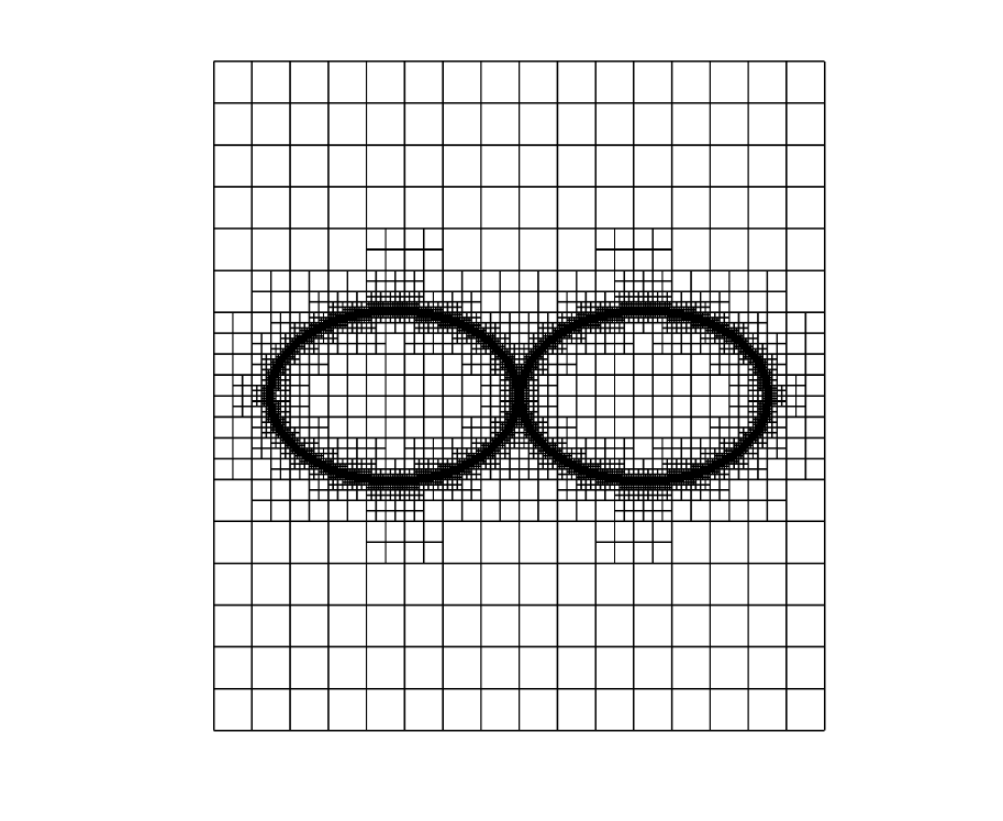
(Wave propagation problem) Let and . We consider the following wave equation with discontinuous coefficients
(6.2)
We assume the interface is the union of two closely located ellipses. We take , which is the union of two disks, and . Here , , , and . The distance between two ellipses is . We consider the wave equation (6.2) with , , and the source is chosen such that the exact solution is
where .
The exact solution is computed by (6.2) with the initial condition .
We use the unfitted finite element method in Chen et al [7] to discretize the problem in space. Let be an induced mesh which is constructed from a Cartesian partition of the domain with possible local refinements and hanging nodes so that the elements are large with respect to both domains . Let and , where .
For any , , let and the polygonal approximation of bounded by the sides of and which is the line segment connecting two intersection points of . is the union of shape regular triangles , , whose sides are the sides of and . We always set the element having as one of its sides. From we define the curved element by
Then we know that is the union of curved triangles , .
For any integers , the space denotes the space of polynomials of degree at most in and denotes the space of polynomials of degree at most for the first variable and for the second variable in . For any , we define the interface finite element spaces
and . Notice that the functions in are conforming in each .
Now we define the following unfitted finite element spaces
Let , where .
The semi-discrete unfitted finite element method for solving (6.2) is then to find such that for all ,
(6.3)
(6.4)
(6.5)
where and are the standard projection operators.
It is shown in [7, Theorem 2.2] that the following energy error of the semi-discrete scheme
has -th order convergence.
The semi-discrete problem (6.3)-(6.5) is an ODE system which is solved by the continuous time Galerkin method in this paper. By Theorem 2.1 and Theorem 2.2, we know that the energy error has convergence rate in the norm and in the at nodes , .
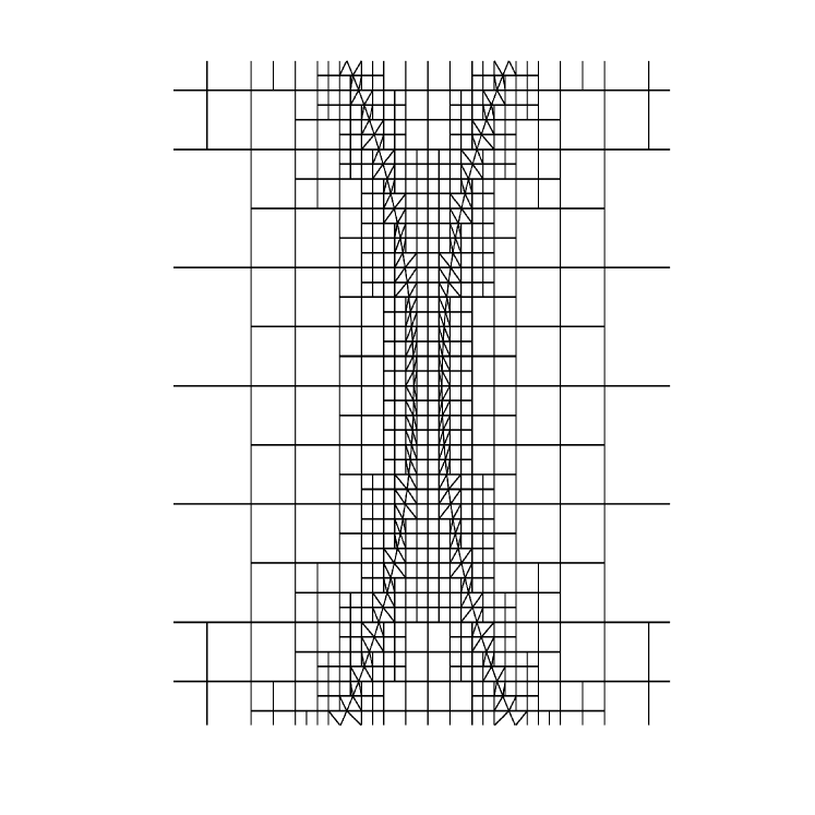
Note that these two ellipses are close but not tangent. To resolve the interface well, we locally refine the mesh near the interface such that the interface deviation for all . For the concept of the interface deviation we refer to [7, Definition 2.2], see also Chen et al [6, Definition 2.2]. As an illustration, we show the computational mesh for in Figure 1.
In this example, we test the accuracy of the error in the norm and . As in Example 1, to test the accuracy at nodes, we set , thus the wall time of using Algorithm 3.1 for the sequential computation is proportion to which minimizes at for , where . Table 3 shows the error at the terminal time when .
To test the accuracy in the norm, we set and thus , where . As in Example 1, the wall time of using Algorithm 3.1 and Algorithm 3.2 for the parallel computation is proportion to which decreases in . However, since the wave equation is not dissipative, we cannot use Algorithm 4.1 for the sequential computation. In this case, the wall time of using Algorithm 3.1 and Algorithm 3.2 for the sequential computation is proportion to which is increasing if and minimizes at if . Since is equivalent to , the optimal choice of the order for minimizing the computation wall time is . Table 3 shows the error
as the approximation of when . We clearly observe the optimal -th order convergence and the superior performance of high order methods from Tables 3-4.
Figure 1: Illustration of the computational domain and the mesh (left) and the corresponding zoomed local mesh (right) with in Example 2.
Table 3: Example 2: numerical errors of and orders.
error
order
error
order
error
order
4.22E-01
–
2.21E-01
–
1.25E-01
–
8.97E-02
2.24
2.64E-02
3.06
6.20E-03
4.33
1.32E-02
2.76
1.81E-03
3.87
3.82E-05
4.96
1.66E-03
2.99
1.13E-04
4.00
1.19E-06
5.00
Table 4: Example 2: numerical errors of and orders.
error
order
error
order
error
order
5.23E-01
–
2.95E-01
–
1.69E-01
–
1.26E-01
2.05
3.70E-02
3.00
8.87E-03
4.25
1.90E-02
2.72
2.58E-03
3.84
2.93E-04
4.92
2.45E-03
2.96
1.66E-04
3.95
9.21E-06
4.99
References
[1]
G. Akrivis, C. Makridakis, and R. H. Nochetto,
Galerkin and Runge-Kutta methods: unified formulation, a posteriori error estimates and nodal superconvergence,
Numer. Math., 118: 429–456, 2011.
[2]
A.K. Aziz and P. Monk,
Continuous finite elements in space and time for the heat equation,
Math. Comp., 52: 255-274, 1989.
[3]
C. Bernardi and Y. Maday,
Spectral methods,
Handbook of Numerical Analysis, 5: 209–485, 1997.
[4]
W.C. Brown,
Matrices over Commutative Rings,Marcel Dekker, New York, 1993.
[5]
J. Chen, Z. Chen, T. Cui, and L. Zhang,
An adaptive finite element method for the eddy current model
with circuit/field couplings,
SIAM J. Sci. Comput., 32: 1020–1042, 2010.
[6]
Z. Chen, K. Li, and X. Xiang,
An adaptive high-order unfitted finite element method for elliptic interface problems,
Numer. Math., 149: 507-548, 2021.
[7]
Z. Chen, Y. Liu, and X. Xiang,
A high order explicit time finite element method for the acoustic wave equation with discontinuous coefficients,
arXiv:2112.02867v2.
[8]
Y. Cheng, X. Meng, and Q. Zhang,
Application of generalized Gauss-Radau projections for the local discontinuous Galerkin method for linear convection-diffusion equations,
Math. Comp., 86: 1233–1267, 2017.
[9]
B. Cockburn and C.-W. Shu,
The local discontinuous Galerkin method for time-dependent convection-diffusion systems,
SIAM J. Numer. Anal., 35: 2440–2463, 1998.
[10]
J. Douglas Jr., T. Dupont, and M.F. Wheeler,
A quasi projection analysis of Galerkin methods for parabolic and hyperbolic equations,
Math. Comp., 32: 345-362, 1978.
[11]
D. A. French and T. E. Peterson,
A continuous space-time finite element method for the wave equation,
Math. Comp., 65: 491–506, 1996.
[12]
E. Gallopoulos, and Y. Saad,
On the parallel solution of parabolic equations,
Proceedings of the 3rd international conference on Supercomputing, 17–28, 1989.
[13]
M.J. Gander,
50 years of time parallel time integration,
in Multiple shooting and time domain decomposition, T. Carraro, M. Geiger, S. Körkel, and R. Rannacher, eds., Springer-Verlag, Berlin, 2015, pp. 69–114.
[14]
G.H. Golub and C.F. Van Loan,
Matrix Computations, third edition,
The John Hopkins University Press, Baltimore, Maryland, 1996
[15]
R. Griesmaier, and P. Monk,
Discretization of the Wave Equation Using Continuous
Elements in Time and a Hybridizable Discontinuous
Galerkin Method in Space,
J. Sci. Comput., 58: 472–498, 2014.
[16]
E. Hairer and G. Wanner,
Solving Ordinary Differential Equations II,Springer-Verlag, Berlin, Heidelberg, 1996.
[17]
B.L. Hulme,
One-step piecewise polynomial Galerkin methods for initial value problems,
Math. Comp., 26: 415–426, 1972.
[18]
O. Perron,
Algebra, Volume II,
Guschens Bücherei, Berlin, 1933.
[19]
T. Richter, A. Springer, and Vexler, Efficient numerical realization of discontinuous Galerkin methods for temporal discretization of parabolic problems, Numer. Math., 124: 151–182, 2013.
[20]
E. B. Saff and R. S. Varga,
On the zeros and Poles of Padé Approximation to ,
Numer. Math., 25: 1–14, 1975.
[21]
D. Schötzau and Ch. Schwab,
p- and hp- Finite Element Methods,Oxford Science Publications, New York, 1998.
[22]
D. Schötzau and Ch. Schwab,
The time discretization of parabolic problems by the hp-version of the discontinuous Galerkin finite element method,
SIAM J. Numer. Anal., 38: 837–875, 2000.
[23]
B.N. Southworth, O. Krzysik, W. Pazner, and H. De Sterck,
Fast solution of fully implicit Runge-Kutta and discontinuous Galerkin in time for numerical PDEs, Part I: The linear setting,
SIAM J. Sci. Comput., 44: A416–A443, 2022.
[24]
G. Szegö,
Orthogonal Polynomials,
American Mathematical Society, New York, 1939.
[25]
Y. Wu and Y. Bai,
Error analysis of energy-preserving mixed finite element methods for the Hodge wave equation,
SIAM J. Numer. Anal., 59: 1433–1454, 2021.