Adaptive quantum error mitigation using pulse-based inverse evolutions

Abstract

^∗raam@mail.huji.ac.il

Quantum Error Mitigation (QEM) enables the extraction of high-quality results from the presently-available noisy quantum computers. In this approach, the effect of the noise on observables of interest can be mitigated using multiple measurements without additional hardware overhead. Unfortunately, current QEM techniques are limited to weak noise or lack scalability. In this work, we introduce a QEM method termed ‘Adaptive KIK’ that adapts to the noise level of the target device, and therefore, can handle moderate-to-strong noise. The implementation of the method is experimentally simple — it does not involve any tomographic information or machine-learning stage, and the number of different quantum circuits to be implemented is independent of the size of the system. Furthermore, we have shown that it can be successfully integrated with randomized compiling for handling both incoherent as well as coherent noise. Our method handles spatially correlated and time-dependent noise which enables to run shots over the scale of days or more despite the fact that noise and calibrations change in time. Finally, we discuss and demonstrate why our results suggest that gate calibration protocols should be revised when using QEM. We demonstrate our findings in the IBM quantum computers and through numerical simulations.

Introduction

Quantum computers have reached a point where they outperform even the most powerful classical computers in specific tasks ^{1; 2; 3}. However, these quantum devices still face considerable noise levels that need to be managed for quantum algorithms to excel in practical applications. Quantum error correction (QEC) is a prominent solution, although its implementation, particularly in complex problems such as Shor’s factoring algorithm, might demand thousands of physical qubits for each encoded logical qubit ^{4; 5}.

A different approach, quantum error mitigation (QEM), has garnered substantial attention recently ^{6; 7; 8; 9; 10; 11; 12; 13; 14; 15; 16; 17; 18; 19; 20; 21; 22; 23}. Its viability has been demonstrated through experiments involving superconducting circuits ^{24; 25; 26; 27; 21; 20; 28; 19; 29}, trapped ions ³⁰, and circuit QED ³¹. QEM protocols aim to estimate ideal expectation values from noisy measurements, without the resource-intensive requirements of QEC. This positions them as potential solutions for achieving quantum advantage in practical computational tasks ^{19; 28}. Some QEM strategies require moderate hardware overheads and can be seen as intermediary solutions between NISQ (Noisy Intermediate-Scale Quantum) computers and devices that fully exploit QEC ^{11; 12}. These strategies aim to virtually refine the pure final state, by utilizing extra qubits for error mitigation without actively correcting errors. The approach introduced here fits into the more common class of QEM techniques that maintain the qubit count of the original circuit.

The objective of QEM is to reduce errors in post processing, rather than fixing them in real time. For instance, the zero-noise extrapolation (ZNE) method ^{6; 7} employs circuits that mimic the ideal target evolution but amplify noise by a controlled factor. The noiseless expectation values are estimated via extrapolation to the zero-noise limit, after fitting a noise scaling ansatz to the measured data. While the construction of circuits that correctly scale the noise is straightforward if the noise is time independent ⁶ or if it is decribed by a global depolarizing channel ¹³, it has been observed that circuits designed to amplify depolarizing noise fail to achieve the intended noise scaling, when applied to more realistic noise models ¹⁹. Our experimental findings also show related issues when applying such circuits to QEM in a real system. Another strategy is to simplify the actual noise appearing in multi-qubit gates such as the CNOT, CZ, Toffoli and Fredkin gates, by using randomized compiling, which renders the noise to a Pauli channel ^{32; 33}. A sufficiently sparse Pauli channel facilitates accurate characterization and noise amplification for ZNE ²⁸. Additionally, as in other QEM methods, the performance of ZNE can be enhanced by integrating it with other error mitigation techniques ³⁴, such as readout error mitigation ¹⁷.

In comparison to ZNE, Probabilistic Error Cancellation (PEC) is a QEM scheme that relies on an experimental characterization of the noise to effectively suppress the associated error channel ^{6; 8; 9; 25; 20}. To this end, PEC uses a Monte Carlo sampling of noisy operations that on average cancel out the noise, thereby providing an unbiased estimation of the noise-free expectation value. However, this objective can only be accomplished when precise and complete tomographic details of the noise process are accessible. In practice, the success of bias suppression in PEC is limited by the scalability and accuracy of gate set tomography in realistic scenarios. Additionally, since noise characteristics evolve over time, the learning process for PEC must be carried out efficiently within a timescale that is shorter than the timescale in which the noise parameters change. A more realistic approach aims for a partial characterization of the noise, using tools like local gate set tomography ⁸ or learning of a sparse noise model ²⁰. The latter strategy was also employed to assist the implementation of ZNE in the experiment of Ref. ²⁸. Alternatively, it is possible to learn a noise model by taking advantage of circuits that are akin to the target circuit but admit an efficient classical simulation ^{9; 10; 16; 35}. By concatenating the outcomes from the ideal (simulated) circuits with their experimental counterparts, the noise-free expectation value can be estimated through some form of data regression ^{10; 35}. Similar learning-based schemes have also been integrated with PEC ⁹ and ZNE ¹⁶.

In this work, we introduce the ‘Adaptive KIK’ method (‘KIK’ for brevity) for handling time dependent and spatially correlated noise in QEM. This technique bears a certain (misleading) similarity to a ZNE variant known as circuit (or ‘global’ ³⁴) unitary folding ¹³, where noise is augmented through identity operations that comprise products of the target evolution and its inverse. While both methods utilize folding to mitigate noise, they differ in the error mitigation mechanism and the way the measured data is processed. Instead of extrapolating to the zero-noise limit, we combine appropriately folded circuits to effectively construct the ‘inverse noise channel’ and approximate the ideal unitary evolution. As opposed to PEC, the implementation of the KIK method does not involve any tomographic information or noise learning subroutine. More precisely, the coefficients that weight the folded circuits are analytically optimized according to a single experimental parameter that probes the intensity of the noise. Another distinctive aspect of KIK mitigation is a specific inversion of the target circuit for the folding procedure. This constitutes a pivotal difference with respect to circuit folding and has practical consequences, as we show experimentally. The combination of a proper inverse and coefficients adapted to the noise strength allows us to mitigate moderate-to-strong noise and significantly outperform circuit folding ZNE in experiments and simulations. Although we show that the weak noise limit of our theory has a clear connection with Richardson ZNE using circuit folding ¹³, the correct inversion of the target circuit is still crucial in this limit.

Recently, important results on the fundamental limitations of QEM protocols have been obtained ^{36; 37}. These studies address the degradation in the statistical precision of generic QEM schemes, as noise accumulates in circuits of increasing size. In this work, instead of analyzing the degradation of statistical precision, our focus is on the accuracy of error mitigation. We obtain upper bounds for the bias between the ideal expectation value of an arbitrary observable and the value estimated using the KIK method, as a function of the accumulated noise. Our bounds show exponential suppression of the bias with respect to the number of foldings when the noise is below a certain threshold. This is in contrast with ZNE schemes which, in general, do not provide accuracy guarantees.

We test the KIK method on a ten-swap circuit and in a CNOT calibration process, using the IBM quantum computing platform. In the ten-swap experiment, we demonstrate the success of our approach for mitigating strong noise. In the calibration experiment, it is illustrated that a noise-induced bias in gate parameters leads to coherent errors. KIK-based calibration can efficiently mitigate these coherent errors by reducing the bias in the calibration measurements. Furthermore, we find that circuit folding (which uses the CNOT as its own inverse) produces erroneous and inconsistent results. Our experimental findings are enhanced by complementing the KIK method with randomized compiling and readout mitigation. We also simulate the fidelity obtained with a noisy ten-step Trotterization ³⁸ of the transverse Ising model on five qubits. For unmitigated fidelities as low as 0.85, we show that KIK error mitigation produces final fidelities beyond 0.99.

Results

The KIK formula for time-dependent noise

To derive our results, we adopt the Liouville-space formalism of Quantum Mechanics ³⁹ (see Supplementary Note 1), in which density matrices that describe quantum states are written as vectors, and quantum operations as matrices that act on these vectors. In the following, we will employ calligraphic fonts to denote quantum operations. For example, the unitary evolution associated with an ideal (noise-free) quantum circuit and its noisy implementation will be written as $\mathcal{U}$ and $\mathcal{K}$, respectively.

In the standard representation involving superoperators and density matrices, the noisy evolution is governed by the equation

$$\frac{d}{dt}\rho=-i[H(t),\rho]+\hat{L}(t)[\rho].$$ (1)

The ideal evolution is generated by the time-dependent Hamiltonian $H(t)$. On the other hand, the effect of noise is characterized by the superoperator $\hat{L}(t)$. In the following, we will refer to this superoperator as the ‘dissipator’. The equivalent of Eq. (1) in Liouville space is the equation

$$\frac{d}{dt}|\rho\rangle=\left(-i\mathcal{H}(t)+\mathcal{L}(t)\right)|\rho\rangle,$$ (2)

where $|\rho\rangle$ is the vectorized form of $\rho$. Moreover, $\mathcal{H}(t)$ and $\mathcal{L}(t)$ are square matrices that represent the Hamiltonian $H(t)$ and the dissipator, respectively. We refer the reader to Supplementary Note 2 for more details.

The dynamics (2) gives rise to the noisy target evolution, which we have denoted by $\mathcal{K}$. As shown in Supplementary Note 3, we can write the solution to Eq. (2) as $\mathcal{K}=\mathcal{U}e^{\Omega(T)}$, where $\Omega(T)=\sum_{n=1}^{\infty}\Omega_{n}(T)$ is the so called Magnus expansion ⁴⁰. The time $T$ is the total evolution time and $\Omega_{n}(T)$ is the $n$th order Magnus term corresponding to $T$. Here, we are specifically interested in the first Magnus term $\Omega_{1}(T)$, for reasons that will be clarified below. In our framework, $\Omega_{1}(T)$ characterizes the impact of noise and is given by

$$\Omega_{1}(T)=\int_{0}^{T}dt\mathcal{U}^{\dagger}(t)\mathcal{L}(t)\mathcal{U}(t),$$ (3)

where $\mathcal{U}(t)$ is the noise-free evolution at time $t$. In particular, $\mathcal{U}:=\mathcal{U}(T)$ is the unitary associated with the noise-free target circuit.

Our basic approximation is the truncation of the Magnus series to first order. This leads to

$$\mathcal{K}\approx\mathcal{U}e^{\Omega_{1}(T)}.$$ (4)

Next, we apply the same approximation to a suitable inverse evolution $\mathcal{K}_{\textrm{I}}$, such that $\mathcal{K}_{\textrm{I}}$ reproduces the unitary $\mathcal{U}^{\dagger}$ in the absence of noise. We construct $\mathcal{K}_{\textrm{I}}$ through an inverse driving $\mathcal{H}_{\textrm{I}}(t)$ defined by

$$\mathcal{H}_{\textrm{I}}(t)=-\mathcal{H}(T-t).$$ (5)

The driving $\mathcal{H}_{\textrm{I}}(t)$ undoes the action of $\mathcal{H}(t)$, and it produces $\mathcal{U}^{\dagger}$. By using $\mathcal{H}_{\textrm{I}}(t)$, we find in Supplementary Note 3 that, to first order in the Magnus expansion, the solution to the corresponding noisy dynamics satisfies

$$\mathcal{K}_{\textrm{I}}\approx e^{\Omega_{1}(T)}\mathcal{U}^{\dagger}.$$ (6)

Note that this approximation does not mean that we keep only the linear term $\Omega_{1}(T)$, since all the powers of $\Omega_{1}(T)$ are included in the exponential $e^{\Omega_{1}(T)}$. In Eqs. (6) and (7), we use the symbol ‘$\approx$’ to denote equality up to the first Magnus term.

The fact that $\Omega_{1}(T)$ is also present in the inverse evolution $\mathcal{K}_{\textrm{I}}$ allows us to express the error channel as $e^{\Omega_{1}(T)}\approx\left(\mathcal{K}_{\textrm{I}}\mathcal{K}\right)^{\frac{1}{2}}$. While $\mathcal{H}_{\textrm{I}}(t)$ is not the only alternative for generating $\mathcal{U}^{\dagger}$, it guarantees the generation of a noise channel that is identical, within our appoximation, to the noise channel of $\mathcal{K}$. Thus, by working within the first-order truncation of the Magnus expansion, we can combine Eqs. (4) and (6) to obtain

$$\mathcal{U} \approx\mathcal{K}e^{-\Omega_{1}(T)}$$

$$\approx\mathcal{K}\left(\mathcal{K}_{\textrm{I}}\mathcal{K}\right)^{-\frac{1}{2}}.$$ (7)

The ‘KIK formula’ in the second line of (7) is our main result. In the next section, we discuss the implementation of the KIK method through polynomial expansions of the operator $\left(\mathcal{K}_{\textrm{I}}\mathcal{K}\right)^{-\frac{1}{2}}$ appearing in this formula.

We stress that until now the only assumption regarding the nature of the noise is that (see Supplementary Note 2)

$$\mathcal{L}_{\textrm{I}}(t)=\mathcal{L}(T-t),$$ (8)

where $\mathcal{L}_{\textrm{I}}(t)$ is the dissipator acting alongside $\mathcal{H}_{\textrm{I}}(t)$. This relationship follows from the form of the driving (5), and is schematically explained in Fig. 1. As detailed in Supplementary Note 2, Eq. (8) relies on the time locality of the noise. That is, on the assumption that the dissipators $\mathcal{L}(t)$ and $\mathcal{L}_{\textrm{I}}(t)$ are only determined by the current time $t$ and not by the previous history of the evolution. Therefore, Eq. (8) may be violated or only hold approximately in the presence of pronounced non Markovian noise.

Due to the generality of $\mathcal{L}(t)$, Eq. (7) is applicable to quantum circuits $\mathcal{K}$ that feature time-dependent and spatially correlated noise, as well as gate-dependent errors. In Supplementary Note 3, we also discuss the scenario where noise parameters drift during the experiment, which occurs for example due to temperature variations or laser instability. We show that the impact of noise drifts can be practically eliminated in our method, if the execution order of the circuits $\mathcal{K}\left(\mathcal{K}_{\textrm{I}}\mathcal{K}\right)^{m}$ in Eq. (9) is properly chosen. As a final remark, we note that the time independent Lindblad master equation ⁴¹ is a special case of Eq. (1). Therefore, our formalism goes beyond QEM proposals based on such a master equation, like the one adopted in Ref. ⁴².

QEM using the KIK formula

Since $\mathcal{K}$$\left(\mathcal{K}_{\textrm{I}}\mathcal{K}\right)^{-\frac{1}{2}}$ is not directly implementable in a quantum device, we utilize polynomial expansions of $\left(\mathcal{K}_{\textrm{I}}\mathcal{K}\right)^{-\frac{1}{2}}$ such that

$${\normalcolor{\color[rgb]{1,0,0}{\normalcolor\mathcal{U}_{\textrm{KIK}}^{(M)}=}}}\sum_{m=0}^{M}a_{m}^{(M)}\mathcal{K}\left(\mathcal{K}_{\textrm{I}}\mathcal{K}\right)^{m}.$$ (9)

The notation $\mathcal{U}_{\textrm{KIK}}^{(M)}$ represents an $M$th-order approximation to $\mathcal{U}_{\textrm{KIK}}$, with real coefficients $\{a_{m}^{(M)}\}_{m=0}^{M}$. In this way, we estimate the error-free expectation of an observable $A$ as

$${\left\langle A\right\rangle_{\textrm{KIK}}^{(M)}=\sum_{m=0}^{M}a_{m}^{(M)}\left\langle A\right\rangle_{m}},$$ (10)

where $\left\langle A\right\rangle_{m}$ is the expectation value measured after executing the circuit $\mathcal{K}\left(\mathcal{K}_{\textrm{I}}\mathcal{K}\right)^{m}$ on the initial state $\rho$. Before discussing the evaluation of the coefficients $a_{m}^{(M)}$, used in Eq. (10), it is instructive to clarify some similarities and differences between the KIK method and ZNE based on circuit folding.

The application of the KIK formula is operationally analogous to the use of circuit folding for ZNE ^{13; 34}. However, there are two crucial differences between these two techniques. Circuit folding is a variant of unitary folding, first introduced in Ref. ¹³ as a user-friendly strategy for noise amplification in ZNE . It operates by inserting quantum gates that are logically equivalent to the identity operation, which leave the noiseless circuit unmodified. In the case of ‘circuit folding’, identities are generated by folding the target circuit with a corresponding inverse circuit. Hence, the noise is scaled through evolutions that have the structure $\mathcal{U}\left(\mathcal{U}^{\dagger}\mathcal{U}\right)^{m}$ ¹³. Notably, excluding the trivial case of a global depolarizing channel ¹³, a rigorous description of how noise manifests when executing $\mathcal{U}\left(\mathcal{U}^{\dagger}\mathcal{U}\right)^{m}$was never presented, to the best of our knowledge. In this sense, circuit folding and other variants of unitary folding can be considered as a heuristic approach to QEM. Upon measuring the observable of interest on these circuits, the noiseless expectation value is estimated by combining the results corresponding to different values of $m$, with weights that depend on the noise scaling ansatz.

The similarity with respect to the KIK method comes from the fact that the circuits $\mathcal{K}\left(\mathcal{K}_{\textrm{I}}\mathcal{K}\right)^{m}$ in Eq. (9) are noisy implementations of $\mathcal{U}\left(\mathcal{U}^{\dagger}\mathcal{U}\right)^{m}$. However, a key difference is that in our case $\mathcal{U}^{\dagger}$ is performed using the driving (5). Hereafter, we shall refer to this implementation as the ‘pulse inverse’. Conversely, unitary folding (and particularly circuit folding) relies on a circuit-based inversion, where gates that are their own inverses are executed in their original form. This is true for both foldings of single gates (or circuit layers) and for circuit foldings. A paradigmatic example would be the CNOT gate. In contrast, the driving (5) reverses the pulse schedule for each gate in the target circuit, including CNOTs and other gates that are their own inverses. This translates into a very distinct execution of $\mathcal{U}^{\dagger}$, as illustrated in Fig. 1(a). Even if $\mathcal{U}$ is just a single CNOT, we show in the section ‘Experimental results’ that properly folded circuits correspond to products between the CNOT and its pulse inverse, while circuit folding (i.e. products of the CNOT with itself) leads to erroneous results. Regarding the implemetation of our method on cloud-based platforms, we are currently writing an open source Qiskit module that generates pulse-inverse circuits automatically, using only gate-level control. Consequently, users will not need to master pulse-level control to utilize our QEM technique.

Figure 1: Illustration of the pulse inverse used in the KIK method. (a) Quantum gates are executed via classical control signals, or ‘pulses’. The left panel shows a pulse schedule used for a CNOT gate in the IBM quantum computing platform. The pulse schedule in the right panel performs the inverse of the CNOT through the inverse driving $\mathcal{H}_{\textrm{I}}(t)$. It is constructed from the original pulse schedule $\mathcal{H}(t)$, by inverting the amplitudes of the pulses (black curved arrow) and their time ordering (red curved arrow). (b) Instead of the pulse inverse, circuit folding and other variants of unitary folding ^{13; 34} use the CNOT as its own inverse. Therefore, the pulse schedule for the inverse evolution is not modified. (c) Noisy implementations of $\mathcal{K}$ and $\mathcal{K}_{\textrm{I}}$. We assume that during the executions of $\mathcal{K}$ and $\mathcal{K}_{\textrm{I}}$ temporal variations of the noise due to external factors (e.g. temperature variations) are negligible. Thus, any time dependence in $\mathcal{L}(t)$ is induced by the time dependence of $\mathcal{H}(t)$. (Top) This leads to gate dependent noise depicted by different border colors in the gates $U_{\textrm{a}}$, $U_{\textrm{b}}$, and $U_{\textrm{c}}$. (Bottom) Since $\mathcal{H}_{\textrm{I}}(t)$ reverses the time ordering of $\mathcal{H}(t)$, the time ordering of $\mathcal{L}(t)$ is also reversed. However, the sign of $\mathcal{L}(t)$ does not change because otherwise the inverse evolution would undo the noise.

Let us now discuss another major difference between our scheme and QEM protocols based on ZNE (including circuit folding). In the case of ZNE, the coefficients that weigh different noise amplification circuits are determined by the fitting of the noise scaling ansatz to experimental data. Rather than that, we ask how to choose these coefficients in such a way that $\mathcal{U}_{\textrm{KIK}}^{(M)}$ constitutes a good approximation to the KIK formula. This problem can be formulated in terms of the eigenvalues of the operators $\left(\mathcal{K}_{\textrm{I}}\mathcal{K}\right)^{-\frac{1}{2}}$ and $\sum_{m=0}^{M}a_{m}^{(M)}\left(\mathcal{K}_{\textrm{I}}\mathcal{K}\right)^{m}$. If $\lambda$ denotes a generic eigenvalue of $\mathcal{K}_{\textrm{I}}\mathcal{K}$, our goal is to find a polynomial $\sum_{m=0}^{M}a_{m}^{(M)}\lambda^{m}$ that is as close as possible to $\lambda^{-1/2}$. Depending on the noise strenght, we follow the two strategies presented in the following two sections. This will further clarify why our method cannot be not considered as a ZNE variant.

QEM in the weak noise regime

In the limit of weak noise, the circuit $\mathcal{K}_{\textrm{I}}\mathcal{K}$ resembles the identity operation and therefore in this case it is reasonable to approximate the function $\lambda^{-\frac{1}{2}}$ by a truncated Taylor series around $\lambda$=1. The resulting Taylor polynomial leads to the Taylor mitigation coefficients $a_{m}^{(M)}$=$a_{\textrm{Tay},m}^{(M)}$, derived in Supplementary Note 4. Explicitly,

$$a_{\textrm{Tay},m}^{(M)}=(-1)^{m}\frac{(2M+1)!!}{2^{M}[(2m+1)m!(M-m)!]}.$$ (11)

In the same supplementary note we show that $a_{\textrm{Tay},m}^{(M)}$ coincide with the coefficients obtained from Richardson ZNE, by assuming that noise scales linearly with respect to $m$. Nevertheless, it is worth stressing that a distinctive characteristic of our approach is the pulse-based inverse $\mathcal{K}_{\textrm{I}}$. As proven in Supplementary Note 4, for gates that satisfy $\mathcal{U}^{2}=\mathcal{I}$, using the circuit-based inverse $\mathcal{K}_{\textrm{I}}=\mathcal{K}$ introduces an additional error term that afflicts $\mathcal{U}_{\textrm{KIK}}^{(M)}$ (cf. Eq. (9)) for any mitigation order $M$. Thus, ignoring the pulse inverse hinders QEM performance in paradigmatic gates such as the CNOT, swap, or Toffoli gate.

As a final remark, we note that circuit folding does not explicitly distinguish between noise amplification using powers of $\mathcal{K}_{\textrm{I}}\mathcal{K}$ or $\mathcal{K}\mathcal{K}_{\textrm{I}}$, as both choices reproduce the identity operation in the absence of noise. However, we show in Supplementary Note 3 that a correct application of the KIK formula involves powers of $\mathcal{K}_{\textrm{I}}\mathcal{K}$.

QEM in the strong noise regime

In this section, we present a strategy to adapt the coefficients $a_{m}^{(M)}$ to the noise strength, for handling moderate or strong noise. To this end, we introduce the quantity

$$\varepsilon_{\textrm{L2}}^{(M)}:=\int_{g(\mu)}^{1}\left(\sum_{m=0}^{M}a_{m}^{(M)}\lambda^{m}-\lambda^{-\frac{1}{2}}\right)^{2}d\lambda,$$ (12)

where $\mu=\textrm{Tr}\left(\rho^{\prime}\rho\right)$, $\rho$ is the initial state, and $\rho^{\prime}$ is the state obtained by evolving $\rho$ with the KIK cycle $\mathcal{K}_{\textrm{I}}\mathcal{K}$.

Let us elaborate on the physical meaning of $\varepsilon_{\textrm{L2}}^{(M)}$. For a pure state $\rho$, $\mu$ is the survival probability under the evolution $\mathcal{K}_{\textrm{I}}\mathcal{K}$. Note that, in this case, $\mu=1$ if $\mathcal{K}_{\textrm{I}}\mathcal{K}=\mathcal{I}$. The lower integration limit $g(\mu)$ in Eq. (12) is a monotonically increasing function of $\mu$, such that $0\leq g(\mu)\leq 1$ for $0\leq\mu\leq 1$ and $g(\mu)=1$ if $\mu=1$. Therefore, $g(\mu)$ serves as a proxy for the intensity of the noise affecting the circuit $\mathcal{K}_{\textrm{I}}\mathcal{K}$. More precisely, $g(\mu)$ represents an approximation to the smallest eigenvalue of $\mathcal{K}_{\textrm{I}}\mathcal{K}$, which equals 1 in the noiseless case. As the noise becomes stronger, both the smallest eigenvalue of $\mathcal{K}_{\textrm{I}}\mathcal{K}$ and $g(\mu)$ get closer to 0, which implies that the interval [$g(\mu)$,1] is representative of the region where all the eigenvalues of $\mathcal{K}_{\textrm{I}}\mathcal{K}$ lie. Now, letting $\lambda$ denote a general eigenvalue of this operator, the eigenvalues of $\left(\mathcal{K}_{\textrm{I}}\mathcal{K}\right)^{-\frac{1}{2}}$ and $\sum_{m=0}^{M}a_{m}^{(M)}\left(\mathcal{K}_{\textrm{I}}\mathcal{K}\right)^{m}$ can be written as $\lambda^{-\frac{1}{2}}$ and $\sum_{m=0}^{M}a_{m}^{(M)}\lambda^{m}$, respectively. Since the integrand of Eq. (12) quantifies the deviation between these quantities, $\varepsilon_{\textrm{L2}}^{(M)}$ represents the total error when using Eq. (9) to approximate the KIK formula (7).

Figures 2(a) and 2(b) illustrate the circuits involved in our adaptive approach to error mitigation. The experimental data comprise the expectation values measured on the noisy circuits $\mathcal{K}(\mathcal{K}_{\textrm{I}}\mathcal{K})^{m}$, shown in Fig. 2(a), and the survival probility $\mu$ (Fig. 2(b)). In the limit weak noise limit, the circuit of Fig. 2(b) is not necessary and the $a_{m}^{(M)}$ become the Taylor coefficients given in Eq. (11) (which can also be obtained by setting $g(\mu)=1$ in the adapted coefficients).

We point out that the L2 norm used to express $\varepsilon_{\textrm{L2}}^{(M)}$ in Eq. (12) is not the only possibility to quantify this error. However, it allows us to greatly simplify the derivation of $a_{m}^{(M)}$. The adaptive aspect of our method is based on the minimization of the error $\varepsilon_{\textrm{L2}}^{(M)}$ with respect to these coefficients, under the condition that $\mathcal{U}_{\textrm{KIK}}^{(M)}$ constitutes a trace-preserving map. In this way, we obtain the ‘adapted’ mitigation coefficients $a_{m}^{(M)}=a_{\textrm{Adap},m}^{(M)}$, which depend on $g(\mu)$ by virtue of Eq. (12) (for brevity, this dependence is not explicit in the notation for the adapted coefficients but it is expressed through the subscript ‘Adap’). In particular, we obtain in Supplementary Note 4 the expressions

$$a_{\textrm{Adap},0}^{(1)} =1+\frac{1}{(1+\sqrt{g})^{3}}+\frac{3}{2(1+\sqrt{g})^{2}},$$ (13)

$$a_{Adap,1}^{(1)} =-\frac{5+3\sqrt{g}}{2(1+\sqrt{g})^{3}},$$ (14)

for $M=1,$ and

$$a_{\textrm{Adap},0}^{(2)} =1+\frac{16}{3(1+\sqrt{g})^{5}}-\frac{14}{3(1+\sqrt{g})^{4}}+\frac{4}{(1+\sqrt{g})^{2}},$$ (15)

$$a_{\textrm{Adap},1}^{(2)} =-4\frac{10+8\sqrt{g}+9g+3g^{\frac{3}{2}}}{3(1+\sqrt{g})^{5}},$$ (16)

$$a_{\textrm{Adap},2}^{(2)} =2\frac{13+5\sqrt{g}}{3(1+\sqrt{g})^{5}},$$ (17)

for $M=2$. The coefficients corresponding to $M=3$ are also derived in the same supplementary note.

Figure 2: Adaptive KIK error mitigation. The estimate $\left\langle A\right\rangle_{\textrm{KIK}}^{(M)}$ of a noiseless expectation value involves the execution of the circuits shown in (a) and (b). In particular, the survival probability $\mu$ is used to evaluate the coefficients $a_{\textrm{Adap},m}^{(M)}[g(\mu)]$, for adaptive error mitigation (see main text for details). The green curve in Figs. (c) and (d) is the plot of $\lambda^{-1/2}$ and it contains the eigenvalues of the operation that effectively suppresess the error channel ( $\left(\mathcal{K}_{\textrm{I}}\mathcal{K}\right)^{-\frac{1}{2}}$ in Eq. (7) ). The black dashed curves represent the polynomial approximations $\sum_{m=0}^{M}a_{m}^{(M)}\lambda^{m}$ that appear in the integrand of (12), for third-order mitigation ($M=3$). The better these approximations, the more accurate the corresponding error mitigation. This accuracy is related to the argument $g(\mu)$ in the optimal coefficients $a_{m}^{(3)}=a_{\textrm{Adap},m}^{(3)}[g(\mu)]$, which are obtained by minimizing (12) over the interval [$g(\mu)$,1]. Figures (c) and (d) correspond to $g(\mu)=\mu^{2}$ and $g(\mu)=\mu$, respectively. In (c), $\lambda^{-1/2}$ is very well approximated by $\sum_{m=0}^{3}a_{\textrm{Adap},m}^{(3)}[\mu^{2}]\lambda^{m}$ in the interval where the eigenvalues of $\left(\mathcal{K}_{I}\mathcal{K}\right)^{-\frac{1}{2}}$are distributed (jagged line in the background). In (d), the interval [$\mu$,1] is too small to cover the full eigenvalue distribution and thus $\sum_{m=0}^{3}a_{\textrm{Adap},m}^{(3)}[\mu]\lambda^{m}$ starts to deviate significantly from the green curve, as shown by the gray ellipse. The red curve corresponds to the Taylor polynomial $\sum_{m=0}^{3}a_{\textrm{Adap},m}^{(3)}[1]\lambda^{m}$ and is the less effective approximation, as seen in both (c) and (d).

According to our previous remarks, we can recover the limit of weak noise by setting $g(\mu)=1$. As expected, in this limit Eqs. (13)-(17) coincide with the coefficients $a_{\textrm{Tay},m}^{(M)}$ in Eq. (11) (and similarly for $M=3$, see Supplementary Note 4).

An important question is how the choice of $g(\mu)$ affects the quality of our adaptive KIK scheme. We consider functions $\{g(\mu)\}=\{1,\mu,\mu^{2}\}$ in the ten-swap experiment presented below, and $\{g(\mu)\}=\{1,\mu,\mu^{2},\mu^{2.5}\}$ for a simulation of the transverse Ising model on five qubits, in Supplementary Note 5. In both cases, we observe that $g(\mu)=1$ is outperformed by the functions that explicitly depend on $\mu$. This shows that the adaptive KIK method consistently produces better results, and demonstrates the usefulness of probing the noise strength through the survival probability $\mu$. For $M$ sufficiently large, the adaptive scheme and the Taylor scheme produce similar results. Yet, the adaptive scheme enables to achieve substantially higher accuracies using lower mitigation orders. This is of key importance in practical applications, as low-order mitigation involves less circuits with lower depth (cf. Eq. (9)) and is therefore more robust to noise drifts. In addition, the approximation of keeping only the first Magnus term becomes less accurates as $M$ increases.

The function $g(\mu)=\mu^{2}$ yields the best error mitigation performance, both in the ten-swap experiment and in the simulation presented in Supplementary Note 5. To understand why this happens, it is instructive to consider Figs. 2(c) and 2(d). These figures show plots of $\lambda^{-1/2}$ (green solid curves), which denotes a generic eigenvalue of the noise inversion operation $\left(\mathcal{K}_{\textrm{I}}\mathcal{K}\right)^{-\frac{1}{2}}$, and the polynomial approximations involved in third-order error mitigation (cf. Eq. (12)). The polynomials with coefficients $a_{\textrm{Tay},m}^{(3)}$ (Taylor mitigation) and coefficients $a_{\textrm{Adap},m}^{(3)}$ (adaptive mitigation) correspond to the red solid and black dashed curves, respectively. The jagged line in the background depicts a possible distribution of the eigenvalues of $\left(\mathcal{K}_{\textrm{I}}\mathcal{K}\right)^{-\frac{1}{2}}$ (the height for a given value of $\lambda$ represents the density of eigenvalues close to that value). In Fig. 2(c), the adapted coefficients are evaluated at $g(\mu)=\mu^{2}$, and the interval [$\mu^{2}$,1] approximately covers the full region where the eigenvalues of $\left(\mathcal{K}_{\textrm{I}}\mathcal{K}\right)^{-\frac{1}{2}}$ are contained. Thus, the associated polynomial constitutes a very good approximation to the curve $\lambda^{-1/2}$, as seen in Fig. 2(c). In contrast, the black curve in Fig. 2(d) corresponds to coefficients $a_{\textrm{Adap},m}^{(3)}$ evaluated at $g(\mu)=\mu$, which leads to a poor approximation outside the interval [$\mu$,1] (area enclosed by the gray ellipse). This behavior sheds light on the advantage provided by $g(\mu)=\mu^{2}$ in our experiments and simulations. Note also that all the polynomials converge as $\lambda$ tends to 1 but the Taylor polynomial (red curve) substantially separates from $\lambda^{-1/2}$ for small $\lambda$.

It is important to remark that Eq. (12) represents a measure of the distance between the polynomial (9) and the KIK formula (7), in terms of the L2 norm. In this expression, we assume that the eigenvalues $\lambda$ of $\mathcal{K}_{\textrm{I}}\mathcal{K}$ are uniformly distributed across the integration interval. This is a conservative approach, given that no information besides $\mu$ is available, and in this sense it is also agnostic to the specific noise structure of $\mathcal{K}_{\textrm{I}}\mathcal{K}$. However, the evaluation of the distance $\varepsilon_{\textrm{L2}}^{(M)}$ could benefit from additional knowledge about the eigenvalue distribution, which can be incorporated through a weight function $w(\lambda)\neq 1$ in the integrand of Eq. (12).

We leave the study of experimental criteria for choosing $g(\mu)$ and the potential improvements that this possibility entails for the KIK method for future work. For example, by considering higher order moments such as $\mu_{2}:=\langle\rho|(\mathcal{K}_{\textrm{I}}\mathcal{K})^{2}|\rho\rangle$ it is possible to devise more systematic choices of $g(\mu)$, e.g. $g(\mu)=\mu-\sqrt{\mu_{2}-\mu^{2}}$. Yet, in the studied examples we observed no significant advantage over the simple heuristic choice $g(\mu)=\mu^{2}$. As for other modifications and improvements, one could also explore the use of norms other than the L2 norm employed in Eq. (12). Furthermore, the approximating polynomial can be determined in a non integral manner. For example, by using Lagrange polynomials or a two-point Taylor expansion ⁴³.

Finally, we remark that, apart from the circuits $\mathcal{K}\left(\mathcal{K}_{\textrm{I}}\mathcal{K}\right)^{m}$, used for the error mitigation itself, the estimation of $\mu$ only involves the additional circuit $\mathcal{K}_{\textrm{I}}\mathcal{K}$. Therefore, our adaptive strategy is not based on any tomographic procedure or noise learning stage. Since $\mu$ is a survival probability, its variance is given by $\mu(1-\mu)$ and has the maximum value 0.25, irrespective of the size of the system. This allows for a scalable evaluation of the coefficients for adaptive KIK mitigation. Once these coefficients are determined, the next step is the estimation of the noise-free expectation value using Eq. (10). In the section ‘Fundamental limits and measurement cost of KIK error mitigation’, we will present the corresponding measurement cost, for $1\leq M\leq 3$, and discuss why and in what sense the KIK method is scalable.

Experimental results

In the experiments described below, the KIK mitigation of noise on the target evolution $\mathcal{K}$ is complemented by an independent mitigation of readout errors and a simple protocol for mitigating the coherent preparation error of the intial state $\rho=|00\rangle\langle 00|$ ⁴⁴. The results of the section ‘Quantum error mitigation in a ten-swap circuit’ also include the application of randomized compiling ³² to the evolutions $\mathcal{K}$ and $\mathcal{K}_{\textrm{I}}$, where circuits logically equivalent to the corresponding ideal evolutions are randomly implemented. This is useful for turning coherent errors into incoherent noise, which can be addressed by our method. Details concerning these experimental methods can be found in Supplementary Note 6.

KIK-based gate calibration for mitigating coherent errors. A usual approach to handle coherent errors in QEM is to first transform them into incoherent errors via randomized compiling ³², and then apply QEM. In this section, we discuss the application of the KIK formula to directly mitigate the coherent errors caused by a faulty calibration of a CNOT gate.

The calibration process involves measurements and adjustments of gate parameters for achieving the results that these measurements would produce in the absence of noise. Since noise affects measured expectation values, the resulting bias leads to incorrect adjustments, i.e. miscalibration. This ‘noise-induced coherent error’ effect may be small in each gate but it builds up to a subtantial error in sufficiently deep circuits. Our idea is to complement the KIK error mitigation for a whole circuit, with a KIK-based calibration of the individual gates.

Figure 3: Calibration curve of the pulse amplitude of a CNOT gate in the IBM processor Jakarta, using the KIK method. In (a) and (b) $\mathcal{K}_{\textrm{I}}$ is given by the pulse inverse and the circuit inverse $\mathcal{K}_{\textrm{I}}=\mathcal{K}$, respectively. The initial state is $\rho=|\psi\rangle\langle\psi|$, with $|\psi\rangle=\frac{1}{\sqrt{2}}\left(|0\rangle+|1\rangle\right)\otimes|0\rangle$. The default amplitude is increased by the factors $F$ shown in the $x$ axis of the figure, and for each factor we apply Eq. (9) to evaluate the expectation value $\left\langle Y_{1}\right\rangle$, where $Y_{1}$ is the $y$-Pauli matrix acting on the target qubit. The factor $F_{\left\langle Y_{1}\right\rangle=0}$ corresponds to the ideal expectation value $\left\langle Y_{1}\right\rangle=0$ and yields the calibrated amplitude. The factors $F_{\left\langle Y_{1}\right\rangle=0}$ associated with the magenta and black dashed lines are different, which indicates a shift in the amplitude obtained without KIK calibration. In Fig. 3(b), we see that the convergence achieved for increasing $M$ in Fig. 3(a) is spoiled by the use of the circuit inverse.

Figure 3 shows the results of our calibration test of a CNOT in the IBM processor Jakarta. We apply the gate on the initial state $\rho=\frac{1}{\sqrt{2}}\left(|0\rangle+|1\rangle\right)\otimes|0\rangle$, and measure the expectation value of the Pauli matrix $Y$ acting on the target qubit (i.e. the qubit prepared in the state $|0\rangle$), denoted by $Y_{1}$. We repeat this procedure for different amplitudes of the cross resonance pulse ⁴⁵, which constitutes the two-qubit interaction in the IBM CNOT implementation. Experimental details can be found in Supplementary Note 6. Each data point of Fig. 3 is obtained by applying Taylor mitigation (i.e. by applying Eq. (10) with the coefficients (11)), for $0\leq M\leq 3$, and linear regression (least squares) is used to determine the line that best fits the experimental data. We also verify that in this case error mitigation with the adapted coefficients $a_{\textrm{Adap},m}^{(M)}$ does not yield a noticeable advantage. This indicates that noise is sufficiently weak, which is further supported by the quick convergence of the lines corresponding to $M\geq 1$ in Fig. 3(a).

Keeping in mind that the calibrated amplitude must reproduce the ideal expectation value ${\color[rgb]{0,0,1}{\normalcolor\left\langle Y_{1}\right\rangle=0}}$, we can see from Fig. 3(a) that the predicted amplitude without QEM ($M=0$) and with QEM are different. Since the CNOT is subjected to stochastic noise, without QEM the measured expectation values will be shifted and the corresponding linear regression results in a calibrated amplitude that is also shifted with respect to the correct value. This is illustrated by the separation between the black and magenta dashed lines in Fig. 3(a). The magenta line represents the calibrated amplitude using KIK error mitigation, while the black one is the amplitude obtained without noise mitigation. Calibration based on the black line leads to a noise-induced coherent error. It is important to stress that the benefit of this calibration procedure would manifest when combined with QEM of the target circuit in which the CNOTs participate. The reason is that the calibrated field is consistent with gates of reduced (stochastic) noise (due to the use of QEM in the calibration process), and therefore it is not useful if the target circuit is implemented without QEM.

In Fig. 3 we also observe that a proper implementation of KIK QEM requires the pulse-based inverse $\mathcal{K}_{\textrm{I}}$ (Fig. 3(a)), performed through the driving (5), while the use of another CNOT for $\mathcal{K}_{\textrm{I}}$ (Fig. 3(b)) does not show the expected convergence as the mitigation order $M$ increases. Note also that although a CNOT is its own inverse in the noiseless scenario, it leads to a coefficient of determination $R^{2}$ whose values show a poor linear fit. This further illustrates the importance of using the pulse inverse instead of the circuit inverse, characteristic of ZNE based on global folding. We point out that odd powers of the CNOT gate are a common choice for the application of local folding ZNE ^{34; 46; 47}, where the goal is to amplify the noise on local sectors of the circuit rather than globally. As such, we believe that in practice this procedure would display inconsistencies similar to those observed in our CNOT experiment. More generally, we show in Supplementary Note 4 that foldings of any self-inverse gate with itself produce a residual error that is not present when the pulse inverse is applied.

Quantum error mitigation in a ten-swap circuit. In Fig. 4(a), we show the results of QEM for a circuit $\mathcal{K}$ given by a sequence of 10 swap gates. The experiments were executed in the IBM quantum processor Quito. The schematic of $\mathcal{K}$ is illustrated in Fig. 4(b).

Figure 4: Experimental QEM in the IBM processor Quito. (a) Error-mitigated survival probability for the circuit of Fig. 4(b), as a function of the mitigation order. The ideal survival probability is 1 (dashed black line). Green and orange curves show QEM adapted to the noise intensity, and the blue curve stands for mitigation assuming weak noise (Taylor mitigation). The thickness of the lines stands for the experimental error bars. We see that Taylor mitigation is outperformed by adapted mitigation. (b) The circuit used in the experiments. Each swap is implemented as a sequence of three CNOTs.

We mitigate errors in the survival probability $\textrm{Tr}\left(\rho\sigma\right)$, where $\sigma$ is the noisy final state that results from applying $\mathcal{K}$ to $\rho$. To perform QEM, we consider the truncated expansion (9) with mitigation orders $1\leq M\leq 3$. The blue curve in Fig. 4(a) corresponds to Taylor mitigation $a_{m}^{(M)}=a_{\textrm{Tay},m}^{(M)}$. Coefficients $a_{m}^{(M)}=a_{\textrm{Adap},m}^{(M)}$ that are adapted with functions $g(\mu)=\mu$ and $g(\mu)=\mu^{2}$ in Eq. (12) give rise to the orange and green curves, respectively. Furthermore, for $\mathcal{K}_{\textrm{I}}$ we perform the pulse inverse according to the pulse schedule described by Eq. (5).

In Fig. 4(a) we observe that the adapted coefficients $a_{\textrm{Adap},m}^{(M)}$ outperform Taylor mitigation. This shows that, beyond the limit of weak noise, QEM can be substantially improved by adapting it to the noise intensity. Within our Magnus truncation approximation, we observe that the ideal survival probability is almost fully recovered. The small residual bias is of order $10^{-3}$ and can be associated with small experimental imperfections (e.g. small errors in the detector calibration), or with the higher-order Magnus terms discarded in our framework. In Supplementary Note 7, we also provide a numerical example where neglecting higher-order Magnus terms leads to an eventual saturation of the QEM accuracy. However, in this example we find that fourth-order QEM ($M=4$) yields a relative error as low as $10^{-4}$, which further illustrates the accuracy achieved by the KIK formula.

Due to experimental limitations, it was not possible to implement the ten-swap circuit using CNOTs calibrated through the KIK method. Specifically, we could not guarantee that calibration circuits and error mitigation circuits would run sequentially, and without the interference of intrinsic (noncontrollable) calibrations of the processor. Moreover, this demonstration requires that all the parameters of the gate are calibrated using the KIK method, and not just the cross resonance amplitude. However, we numerically verify in Supplementary Note 6 that coherent errors vanish for a gate calibrated using KIK QEM, to the point that randomized compiling is no longer needed.

Fundamental limits and measurement cost of KIK error mitigation

Fundamental limits of KIK error mitigation. The performance of QEM protocols is often analyzed using two figures of merit. One of them is the bias between the noisy expectation value of an observable and its ideal counterpart, and the other is the statistical precision of the error-mitigated expectation value. The bias defines the QEM accuracy and is evaluated in the limit of infinite measurements. However, any experiment has a limited precision because it always involves a finite number of samples. In QEM protocols, the estimation of ideal expectation values is usually accompanied by an increment of statistical uncertainty, which can be exponential in worst-case scenarios ^{36; 37}. This results in a sampling overhead for achieving a given precision, as compared to the number of samples required without using QEM.

In Supplementary Note 8, we derive the accuracy bounds

$$\varepsilon_{\textrm{KIK}}^{(M)} \leq\sqrt{\textrm{Tr}\left(A^{2}\right)-\frac{\left[\textrm{Tr}\left(A\right)\right]^{2}}{\textrm{Tr}\left(I\right)}}\left|1-\sum_{m=0}^{M}{\color[rgb]{1,0,0}{\normalcolor a_{\textrm{Adap},m}^{(M)}}}(\mu)e^{-2(m+1/2)\intop_{0}^{T}\left\|\mathcal{L}(t)\right\|dt}\right|,\textrm{for }M=1,2,3,$$ (18)

$$\leq\sqrt{\textrm{Tr}\left(A^{2}\right)-\frac{\left[\textrm{Tr}\left(A\right)\right]^{2}}{\textrm{Tr}\left(I\right)}}\left|1-\sum_{m=0}^{M}{\color[rgb]{1,0,0}{\normalcolor a_{\textrm{Adap},m}^{(M)}}}(1)e^{-2(m+1/2)\intop_{0}^{T}\left\|\mathcal{L}(t)\right\|dt}\right|,\textrm{{for }}M=1,2,3,$$ (19)

$$\leq\frac{(2M+1)!!}{2^{M+1}(M+1)!}\sqrt{\textrm{Tr}\left(A^{2}\right)-\frac{\left[\textrm{Tr}\left(A\right)\right]^{2}}{\textrm{Tr}\left(I\right)}}\left(e^{2\intop_{0}^{T}\left\|\mathcal{L}(t)\right\|dt}-1\right)^{M+1}.$$ (20)

These are upper bounds on the bias $\varepsilon_{\textrm{KIK}}^{(M)}$, for an arbitrary observable $A$ and an arbitrary initial state. We also note that the only approximation in Eqs. (18)-(20) and any of our derivations is the truncation of the Magnus expansion to its dominant term. Importantly, this does not exclude errors of moderate or strong magnitude associated with such a term. On the other hand, discarding Magnus terms beyond first order naturally leads to a saturation of accuracy. Such a saturation manifests in a residual bias that cannot be reduced by indefinitely increasing the mitigation order. Therefore, for the tighter bounds (18) and (19) we restrict ourselves to the mitigation orders used in our experiments and simulations, given by $1\leq M\leq 3$.

On the other hand, the loosest bound (20) provides a clearer picture of how the bias associated with the first Magnus term is suppressed by increasing $M$. The quantity $\int_{0}^{T}\left\|\mathcal{L}(t)\right\|dt$ is the integral of the spectral norm of the dissipator $\left\|\mathcal{L}(t)\right\|$, over the total evolution time $(0,T)$. This parameter serves as a quantifier of the noise accumulated during the execution of the target evolution $\mathcal{K}$. Since $\frac{(2M+1)!!}{2^{M+1}(M+1)!}\leq\frac{3}{8}$, Eq. (20) implies that $\varepsilon_{KIK}^{(M)}$ is exponentially suppressed if the accumulated noise is such that

$$e^{2\int_{0}^{T}\left\|\mathcal{L}(t)\right\|dt}<2.$$ (21)

In the case of noise acting locally on individual gates, $\mathcal{L}(t)$ is given by a sum of local dissipators and one can show that $\left\|\mathcal{L}(t)\right\|$ is upper bounded by the summation of all the gate errors in the circuit.

We remark that, in the NISQ era, errors escalate in quantum algorithms due to the lack of QEC. Thus, NISQ computers can perform useful computations only if the accumulated noise $\int_{0}^{T}\left\|\mathcal{L}(t)\right\|dt$ is below a certain value. Our notion of scalabitility is that under the contraint of moderate acumulated noise the KIK method is scale independent. In particular, when $\int_{0}^{T}\left\|\mathcal{L}(t)\right\|dt$ is sufficiently small to satisfy Eq. (21), the exponential error mitigation referred above is applicable to circuits of any size and topology. While achieving a low accumulated noise in big circuits is technologically challenging, if this condition is met the KIK method and the resources that it requires are agnostic to the size of the circuit. Moreover, it is worth noting that Eq. (21) represents a sufficient condition for scalable error mitigation. The possibility of extending this scalability to values of $\int_{0}^{T}\left\|\mathcal{L}(t)\right\|dt$ that violate Eq. (21) depends on the tightness of the accuracy bounds (18)-(20), and constitutes an open problem.

Equations (18)-(20) are applicable to both adaptive mitigation and Taylor mitigation. In contrast, the tightest bound (18) is exclusive of adaptive mitigation. The coefficients $a_{\textrm{Adap},m}^{(M)}$ in this bound are evaluated at $g(\mu)=\mu$. Importantly, (18) is upper bounded by (19) and (20) for any $0\leq\mu\leq 1$, as proven in Supplementary Note 8. According to our experiments and simulations, we believe that even tighter bounds can be obtained for $g(\mu)=\mu^{2}$ or other choices of $g(\mu)$. This topic is left for future investigation.

Lastly, we stress that the condition (21) does not imply that the KIK method is restricted to error mitigation for weak noise. This is related to the reiterated fact that Eqs. (18)-(20) and particularly (20) probably overestimate the actual bias between the error-mitigated expectation value and its ideal counterpart. More importantly, we have shown experimentally and numerically the substantial advantage achieved by the adaptive KIK strategy, as compared to QEM under the assumption of weak noise. This further indicates that the regime of validity of our method likely goes beyond the prediction of Eq. (20).

Measurement cost of KIK error mitigation. For the sampling overhead, we adopt the variance as the measure of statistical precision. Let $\textrm{Var}_{0}\left(A\right)$ denote the variance in the estimation of the expectation value $\left\langle A\right\rangle$, without using error mitigation, and $\textrm{Var}_{M}\left(A\right)$ the variance associated with KIK mitigation of order $M\geq 1$. The sampling overhead is defined as the increment in the number of samples needed to achieve the same precision as in the unmitigated case. Suppose that $N$ measurements constitute the shot budget for KIK mitigation. For a given value of $M$, the sampling overhead is evaluated by minimizing $\textrm{Var}_{M}\left(A\right)$ over the distribution of measurements between the different circuits $\mathcal{K}\left(\mathcal{K}_{\textrm{I}}\mathcal{K}\right)^{m}$. If $N_{m}$ measurements are allocated to $\mathcal{K}\left(\mathcal{K}_{\textrm{I}}\mathcal{K}\right)^{m}$, then

$$\textrm{Var}_{M}\left(A\right)=\sum_{m=0}^{M}\left(a_{m}^{(M)}(g)\right)^{2}\frac{\textrm{var}_{m}\left(A\right)}{N_{m}},,$$ (22)

where $\textrm{var}_{m}\left(A\right)$ denotes the variance that results from measuring $A$ on the circuit $\mathcal{K}\left(\mathcal{K}_{I}\mathcal{K}\right)^{m}$.

Taking into account the constraint $\sum_{m=0}^{M}N_{m}=N$, the minimization of Eq. (22) with respect to $\{N_{m}\}_{m}$ yields $N_{m}=\left|a_{m}^{(M)}\right|N$. Of course, these values have to approximated to the closest integer in practice. Now, we assume that $\textrm{var}_{m}\left(A\right)=\textrm{var}_{n}\left(A\right)$ for all $0\leq m,n\leq M$. Since, for reasons previously discussed, we are interested in low mitigation orders $1\leq M\leq 3$, $\left(\mathcal{K}_{\textrm{I}}\mathcal{K}\right)^{m}$ does not deviate too much from the identity operation and therefore the assumption stated above is reasonable. In this way, replacing $N_{m}=\left|a_{m}^{(M)}\right|N$ into Eq. (22) yields

$$\textrm{Var}_{M}\left(A\right)=\sum_{m=0}^{M}\left|a_{m}^{(M)}(g)\right|\frac{\textrm{var}_{0}\left(A\right)}{N}.$$ (23)

The quantity $\frac{\textrm{var}_{0}\left(A\right)}{N}$ is the variance obtained without using error mitigation. Accordingly,

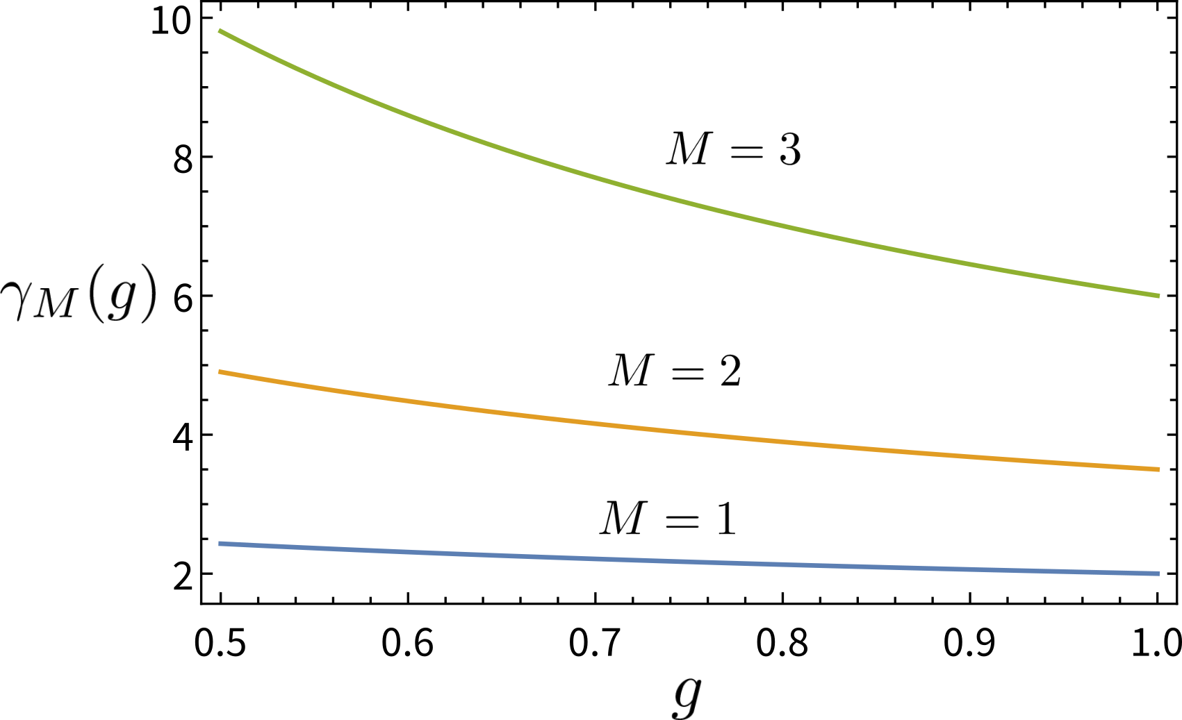
Figure 5: Variance overhead $\gamma_{M}(g)$ of KIK error mitigation, for mitigation orders $1\leq M\leq 3$. The graph shows $\gamma_{M}(g)$ in terms of the function $g=g(\mu)$, used to evaluate the adaptive coefficients $a_{m}^{(M)}(g)$ (cf. Eq. (24)). The overheads for the Taylor coefficients (low noise limit) correspond to the values at $g=1$.

$$\gamma_{M}(g)=\sum_{m=0}^{M}\left|a_{m}^{(M)}(g)\right|$$ (24)

represents the sampling overhead. In Fig. 5, we show the sampling overheads for $1\leq M\leq 3$, as a function of $g=g(\mu)$. As expected, larger noise strengths (corresponding to smaller values of $g$) lead to larger values of $\gamma_{M}(g)$. However, as shown in Fig. 5, these sampling overheads are quite moderate and do not represent an obstacle for scalable error mitigation. In addition, we show in Supplementary Note 3 that our method is robust to noise drifts and miscalibrations that may result from larger sampling overheads, e.g. when higher mitigation orders ($M\geq 4$) are considered.

Discussion

Quantum error mitigation (QEM) is becoming a standard practice in NISQ experiments. However, QEM methods that are free from intrinsic scalability issues lack a physically rigorous formulation, or are unable to cope with significant levels of noise. The KIK method allows for scalable QEM whenever the noise accumulated in the target circuit is not too high, as implied by our upper bounds on the QEM accuracy (cf. Eqs. (18)-(20)). This QEM technique is based on a master equation analysis that incorporates time-dependent and spatially correlated noise, and does not require that the noise is trace-preserving. As such, based on elementary simulations we observe that it can also mitigate leakage noise, which can take place in superconducting circuits. In the limit of weak noise, the KIK method reproduces some features of zero noise extrapolation using circuit unitary folding, and outperforms it. This is achieved thanks to the use of pulse-based inverses for the implementation of QEM circuits, and the adaptation of QEM parameters to the noise intensity for handling moderate and strong noise.

The shot overhead of our method depends only on the noise level and not on the size of the target circuit. For moderate noise, the sampling overhead for mitigation order three or lower is smaller than ten. While the KIK method can be adapted to the strength of the noise, this only requires measuring a single experimental parameter whose sampling cost is negligible and independent of the size of the system. Usually, the performace of QEM techniques may be compromised in experiments involving a large number of samples. When considering long runs, the system needs to be recalibrated multiple times, and noise parameters can undergo significant drifts. This poses challenges in the context of noise learning for QEM protocols that rely on this approach. We show in Supplementary Note 3 that our approach is resilient to drifts in the noise and calibration parameters (the latter holds if randomized compiling is applied). This enables it to be applied in calculations over runtimes of days or even weeks, including pauses for calibrations, maintenance, or execution of supporting jobs. On a similar basis, it is possible to parallelize the error mitigation task, by averaging over data collected from different quantum processors or platforms with spatially differentiated noise profiles (see Supplementary Note 3).

We have demonstrated our findings using the IBM quantum processors Quito and Jakarta. In Quito, we implemented KIK error mitigation in a circuit composed of 10 swap gates (30 sequential CNOTs). Despite the substantial noise in this setup, the tiny bias between the error-mitigated expectation value and the ideal result demonstrates that, at least in this experiment, our theoretical approximations are quite consistent with the actual noise in the system. Using the processor Jakarta, we also showed that even the calibration of a basic building block of quantum computing, such as the CNOT gate, can be affected by unmitigated noise. As a consequence, calibrated gate parameters feature erroneous values leading to coherent errors. These errors can be avoided by incorporating the KIK method in the calibration process. The integration of randomized compiling into our technique also enables the mitigation of coherent errors in the CNOT gates. This is possible because randomized compiling transforms coherent errors into incoherent noise, which can be addressed by the KIK method.

Despite these successful demonstrations, we believe that there is room for improvement by exploring some of the possibilities mentioned in the section ‘QEM in the strong noise regime’. We also hope that the performance shown here can be exploited for new demonstrations of quantum algorithms on NISQ devices, with the potential of achieving quantum advantage in applications of interest.

Data availability

Code employed in the execution of the experiments as well as raw experimental data and data underlying figures is hosted at http://dx.doi.org/10.5281/zenodo.7652322. All additional data are provided in the supplementary information.

Author contributions

Raam Uzdin conceived the method, set the theoretical framework, including most of the analytical derivations, and performed numerical simulations. Jader P. Santos designed and executed the experiments, and performed numerical simulations. Ivan Henao derived some theoretical results, in particular the performance bounds. All the authors were involved in the analysis of theoretical and experimental results, and in the writing and presentation of the paper.

Competing interests

The authors declare no competing financial or non-financial interests.

Adaptive quantum error mitigation using pulse-based inverse evolutions Ivan Henao¹

Jader P. Santos¹

Raam Uzdin¹

Supplementary Note 1: Quantum mechanics in Liouville space

In the standard description of Quantum Mechanics, a system of dimension $d$ is represented by a density matrix $\rho$ of dimension $d\times d$. Moreover, a CPTP (completely positive and trace preserving) quantum operation can be expressed as

$$\rho^{\prime}=\sum_{i}K_{i}\rho K_{i}^{\dagger},$$ (1)

where $\rho^{\prime}$ is a density matrix and $\{K_{i}\}$ are Kraus operators that satisfy the completeness relation $\sum_{i}K_{i}^{\dagger}K_{i}=I$, and $I$ is the $d\times d$ identity matrix. Observables correspond to hermitian operators $A$, and the associated expectation value for a system in a state $\rho$ reads

$$\left\langle A\right\rangle=\textrm{Tr}\left(A\rho\right).$$ (2)

The Liouville space formalism is an alternative formulation that is particularly useful to simplify notation and handle quantum operations. In this framework, a density matrix is replaced by a vector $|\rho\rangle$ of dimension $d^{2}$ and a quantum operation is a matrix of dimension $d^{2}\times d^{2}$. Using the calligraphic notation $\mathcal{O}$ for a quantum operation, the analogous of Eq. (1) in Liouville space is given by

$$|\rho^{\prime}\rangle=\mathcal{\mathcal{O}}|\rho\rangle.$$ (3)

Here, we adopt the approach of Ref. ³⁹, where $|\rho\rangle$ is the column vector whose first $d$ components correspond to the first row of $\rho$, the next $d$ components correspond to the second row of $\rho$, and so forth. More formally, the vector representation of a $d\times d$ generic matrix $B$ (not necessarily a density matrix) is given by $|B\rangle=\left(B_{11},B_{12},...,B_{1d},B_{21},B_{22},...,B_{2d},...,B_{d1},B_{d2},...,B_{dd}\right)^{\textrm{T}}$, where $B_{ij}$ is the $ij$ entry of $B$. With this convention, in Liouville space the quantum operation (1) takes the form ³⁹

$$|\rho^{\prime}\rangle=\sum_{i}K_{i}\otimes K_{i}^{\ast}|\rho\rangle,$$ (4)

where $K_{i}^{\ast}$ is the element-wise complex conjugate of $K_{i}$. For example, a unitary operation $\rho^{\prime}=U\rho U^{\dagger}$ is written as $|\rho^{\prime}\rangle=\mathcal{U}|\rho\rangle$, where $\mathcal{U}=U\otimes U^{\ast}$.

Equation (4) is obtained by following the rule to vectorize a product of three matrices $B$, $C$ and $D$. Denoting the associated vector as $|BCD\rangle$, this rule states that ³⁹

$$|BCD\rangle=B\otimes D^{\textrm{T}}|C\rangle,$$ (5)

where the superscript T denotes transposition. Setting $B=K_{i}$, $C=\rho$, and $D=K_{i}^{\dagger}$, Eq. (4) follows by applying (5) to (1) and using the linearity property of the vectorization.

Finally, to express the expectation value (2) in Liouville space one writes $A$ as a row vector $\langle A|$ defined by $\langle A|=\left(A_{11}^{\ast},A_{12}^{\ast},...,A_{1d}^{\ast},...,A_{d1}^{\ast},A_{d2}^{\ast},...,A_{dd}^{\ast}\right)$. In this way, the hermiticity of $A$ leads to

$$\langle A|\rho\rangle =\sum_{i,j}A_{ij}^{*}\rho_{ij}$$

$$=\sum_{i,j}A_{ji}\rho_{ij}$$

$$=\langle A\rangle.$$ (6)

Supplementary Note 2: Dynamical description of noise for the target evolution and its inverse

In this section, we set the framework for the derivation of the KIK formula (Eq. (1) in the main text). For the sake of clarity and completness, we will discuss again some topics addressed in the main text and rewrite a few equations that were already introduced. We consider a continuous-time description of the system evolution, modeled by the master equation

$$\frac{d}{dt}\rho=-i[H(t),\rho]+\hat{L}(t)[\rho].$$ (7)

Here, $H(t)$ is a time-dependent Hamiltonian and $\hat{L}(t)$ is a time-dependent dissipator that accounts for the non-unitary contribution to the dynamics, which is induced by external noise. The hat symbol in $\hat{L}(t)$ is used to emphasize that it represents a superoperator in Hilbert space.

To specify the form of $\hat{L}(t)$ one could invoke a microscopic description of the dynamics, where the system is coupled to some external environment and the total system obeys the Schrodinger equation. The time-independent case is extensively studied in ⁴¹, and various time-dependent Markovian master equations have been derived ⁴⁸. The dissipator is often given in the Lindblad form, which represents the most general dissipator for a Markovian and CPTP evolution. For our purposes, this is not necessary. For example, $\hat{L}(t)$ could incorporate leakage noise, which does not preserve probability and thus is not trace preserving.

Now, let us rewrite Eq. (7) in Liouville space. Using the linearity of the vectorization operation, we have that

$$\frac{d}{dt}|\rho\rangle=-i|[H(t),\rho]\rangle+|\hat{L}(t)[\rho]\rangle,$$ (8)

where $|[H(t),\rho]\rangle$ and $|\hat{L}(t)[\rho]\rangle$ are the vectors corresponding to $[H(t),\rho]$ and $\hat{L}(t)[\rho]$, respectively. By applying the rule (5) to the commutator $[H(t),\rho]=H(t)\rho-\rho H(t)$, we obtain

$$|[H(t),\rho]\rangle =|H(t)\rho\rangle-|\rho H(t)\rangle$$

$$=\left(H(t)\otimes I-I\otimes H(t)^{\textrm{T}}\right)|\rho\rangle$$

$$:=\mathcal{H}(t)|\rho\rangle,$$ (9)

where $D$ is identified with the identity $I$ for the product $H(t)\rho$, and with $H(t)$ for $\rho H(t)$. In both cases, $C$ is associated with $\rho$. For a general dissipator $\hat{L}(t)$ we can simply write $|\hat{L}(t)[\rho]\rangle=\mathcal{L}(t)|\rho\rangle$, because $\rho$ can always be associated with $C$ in Eq. (5).

In this way, the Liouville-space representation of (7) reads

$$\frac{d}{dt}|\rho\rangle=\left(-i\mathcal{H}(t)+\mathcal{L}(t)\right)|\rho\rangle.$$ (10)

We note that both $\mathcal{H}(t)$ and $\mathcal{L}(t)$ are linear operators that correspond to matrices of dimension $d^{2}\times d^{2}$. While we do not impose any physical constraint on $\mathcal{L}(t)$, in what follows we introduce and physically justify a relationship between $\mathcal{L}(t)$ and the dissipator that affects the pulse inverse evolution. This relationship is crucial for the derivation of the KIK formula in Supplementary Note 3.

Noise for pulse-based inverse evolution. Suppose that applying the driving $\mathcal{H}(t)$ in Eq. (10) during a total time $T$ leads to an ideal unitary evolution $\mathcal{U}=\mathcal{T}e^{-\int_{0}^{T}i\mathcal{H}(t)dt}$, where $\mathcal{T}$ is the time-ordering operator. Even in the circuit model of quantum computing, where unitary operations are composed of discrete quantum gates, each elementary gate is itself generated by a pulse schedule that can be represented as a time-dependent Hamiltonian. Hence, any quantum circuit is ultimately generated by some pulse schedule $\mathcal{H}(t)$.

Different pulse schedules can result in the same ideal evolution $\mathcal{U}$, and naturally the same is true for its inverse $\mathcal{U}^{\dagger}$. However, in the presence of noise this equivalence does not hold in general. The derivation of the KIK formula relies on relating the pulse schedule for $\mathcal{U}^{\dagger}$ with the pulse schedule for $\mathcal{U}$ in a specific manner. Denoting the driving that generates $\mathcal{U}^{\dagger}$ by $\mathcal{H}_{\textrm{I}}(t)$, this relationship reads

$$\mathcal{H}_{\textrm{I}}(t)=-\mathcal{H}(T-t).$$ (11)

In combination with Eq. (11), the other ingredient for obtaining the KIK formula has to do with how noise comes into play for a given driving $\mathcal{H}(t)$. On the one hand, Eq. (10) describes noise that acts locally in time, i.e. that $\mathcal{L}(t)$ only depends on the current instant $t$ and not on the previous history of the evolution. On the other hand, this time dependence can have two origins. One of them is the time-dependence of $\mathcal{H}(t)$ itself, and the other are intrinsic fluctuations of the noise that are related e.g. to changes in the environment or miscalibrations that occur during the execution of an experiment. The second possibility is discussed in detail in Supplementary Note 3. As for the influence of the driving $\mathcal{H}(t)$ on the noise, we assume that $\mathcal{L}(t)$ does not depend on the sign of $\mathcal{H}(t)$, but only on its amplitude. This reflects the fact that noise cannot be undone when running the reverse schedule described in Eq. (11). Taking into account (11), the dissipator $\mathcal{L}_{\textrm{I}}(t)$ for the “pulse inverse” $\mathcal{H}_{\textrm{I}}(t)$ should then satisfy

$$\mathcal{L}_{\textrm{I}}(t)=\mathcal{L}(T-t).$$ (12)

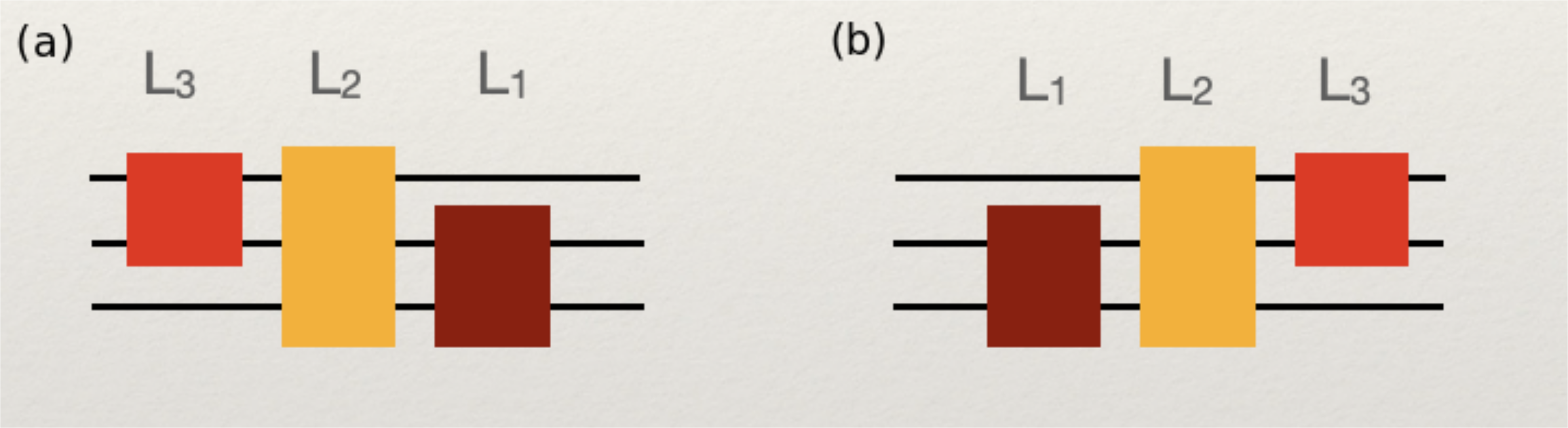
Supplementary Figure 1: Time dependence of dissipators $\mathcal{L}(t)$ and $\mathcal{L}_{\textrm{I}}(t)$. (a) Illustrative noisy quantum circuit, composed of three gates that act on three qubits. The total dissipator $\mathcal{L}(t)$ is given by a sequence of dissipators $\mathcal{L}_{i}$, $1\leq i\leq 3$, which affect each gate. (b) Upon reversing the drive pulse schedule (cf. Eq. (11)), the order of the gates and the corresponding dissipators is also reversed. Hence, if the sequence of dissipators in (a) is $\mathcal{L}_{1}\mathcal{L}_{2}\mathcal{L}_{3}$, in (b) it is given by $\mathcal{L}_{3}\mathcal{L}_{2}\mathcal{L}_{1}$.

Equation (12) implies that if different gates are affected by different noise mechanisms (e.g. very fast gates may be prone to leakage noise due to non-adiabatic couplings to the levels outside the computational basis), the order in which these noise mechanisms operate is reversed when applying the pulse inverse (11), as shown in Supplementary Figure 1. This is a consequence of the time locality of both $\mathcal{L}(t)$ and $\mathcal{L}_{\textrm{I}}(t)$, and the reversed time schedule that $\mathcal{H}_{\textrm{I}}(t)$ imprints on the corresponding inverse gates. To summarize, our sole assumptions on the noise are:

1. The linearity and the time locality of the dissipator $\mathcal{L}(t)$.

2. The relationship between the dissipator $\mathcal{L}_{\textrm{I}}(t)$, which affects the pulse inverse $\mathcal{H}_{\textrm{I}}(t)$ (cf. Eq. (11)) at time $t$, and $\mathcal{L}(t)$. This relationship is encapsulated by Eq. (12).

We remark that $\mathcal{L}(t)$ is not restricted to have a Lindblad form or to give rise to a trace preserving map. For example, it can incorporate leakage noise, which does not conserve the total probability and therefore is not trace preserving.

Following Eq. (10), the noisy evolutions $\mathcal{K}$ and $\mathcal{K}_{\textrm{I}}$ that appear in the KIK formula are thus given by

$$\mathcal{K} =\mathcal{T}e^{\int_{0}^{T}(-i\mathcal{H}(t)+\mathcal{L}(t))dt},$$ (13)

$$\mathcal{K}_{\textrm{I}} =\mathcal{T}e^{\int_{0}^{T}(-i\mathcal{H}_{\textrm{I}}(t)+\mathcal{L}_{\textrm{I}}(t))dt}.$$ (14)

It is important to remark that no restrictions are imposed on the pulse $\mathcal{H}(t)$, so long as it reproduces the noise-free evolution $\mathcal{U}$. On the other hand, we will see in Supplementary Note 3 that Eqs. (11) and (12) allow us to approximate the noise channel for $\mathcal{K}$ as $\left(\mathcal{K}_{\textrm{I}}\mathcal{K}\right)^{\frac{1}{2}}$, which is why the form of the inverse driving in (11) is important for our main finding.

We also note that the level of control required for implementing $\mathcal{H}_{\textrm{I}}(t)$ is very similar to that used for $\mathcal{H}(t)$. In essence, we only need to time-reverse the pulse schedule corresponding to $\mathcal{H}(t)$ and flip its sign. In this work, we use the pulse-gate capabilities of the IBM processors to implement $\mathcal{H}_{\textrm{I}}(t)$. No stretching of the pulses or any modification of their shape is involved. Therefore, the powers of $\mathcal{K}_{\textrm{I}}\mathcal{K}$ that enter the implementation of the KIK method are basically as easy to execute $\mathcal{K}$ itself.

Supplementary Note 3: Derivation of the KIK formula

In this section, we derive the KIK formula

$$\mathcal{U}_{\textrm{KIK}}=\mathcal{K}\left(\mathcal{K}_{\textrm{I}}\mathcal{K}\right)^{-\frac{1}{2}},$$ (15)

where $\mathcal{U}_{\textrm{KIK}}$ is a first-order Magnus approximation to the ideal evolution $\mathcal{U}$ that we will clarify in what follows. Hereafter, we will refer to $\mathcal{K}$ and $\mathcal{K}_{\textrm{I}}$ as target evolution and inverse evolution, respectively. In particular, $\mathcal{K}$ is the noisy evolution over which we intend to perform error mitigation. For now, we assume that the noise-free unitary is given by $\mathcal{U}=\mathcal{T}e^{-\int_{0}^{T}i\mathcal{H}(t)dt}$, meaning that the pulse schedule $\mathcal{H}(t)$ is perfectly calibrated. Hence, the KIK formula is useful to mitigate errors caused by the dissipator $\mathcal{L}(t)$. On the other hand, we will see in Supplementary Note 6 that randomized compiling ³² complements and enhances the error mitigation achieved with the KIK method. Accordingly, integrating randomized compiling into our QEM technique also allows for the mitigation of coherent errors, related to miscalibrations of $\mathcal{H}(t)$.

To arrive at Eq. (15) we shall proceed as follows. We consider that the driving $\mathcal{H}(t)$ acts in the time interval $(0,T)$ and the driving $\mathcal{H}_{\textrm{I}}(t)$ is applied in the interval $(T,2T)$. Thus, the total evolution at time $t=2T$ is $\mathcal{K}_{\textrm{I }}\mathcal{K}$. For any time $t\in(0,2T)$ the dynamics is modeled according to

$$\frac{d}{dt}|\rho\rangle=\left(-i\tilde{\mathcal{H}}(t)+\tilde{\mathcal{L}}(t)\right)|\rho\rangle,$$ (16)

where

$$\tilde{\mathcal{H}}(t) =\begin{cases}\begin{array}[]{c}\mathcal{H}(t)\textrm{ for }t\in(0,T)\\ \mathcal{H}_{\textrm{I}}(t-T)\textrm{ for }t\in(T,2T),\end{array}\end{cases}$$

$$\tilde{\mathcal{L}}(t) =\begin{cases}\begin{array}[]{c}\mathcal{L}(t)\textrm{ for }t\in(0,T)\\ \mathcal{L}_{\textrm{I}}(t-T)\textrm{ for }t\in(T,2T).\end{array}\end{cases}$$ (17)

Note that the action of $\mathcal{H}_{\textrm{I}}$ and $\mathcal{L}_{\textrm{I }}$ on $(T,2T)$ requires the time shift by $T$ as described in Eqs. (17). With this notation, the ideal evolution for $t\in(0,2T)$ is given by $\tilde{\mathcal{U}}(t)=\mathcal{T}e^{-i\int_{0}^{t}\mathcal{\tilde{\mathcal{H}}}(t^{\prime})dt^{\prime}}$, and therefore, $\tilde{\mathcal{U}}(T)=\mathcal{U}$, and $\tilde{\mathcal{U}}(2T)=\mathcal{I}$. Similarly, for the noisy evolution we have that $\tilde{\mathcal{K}}(t)=\mathcal{T}e^{\int_{0}^{t}\left(-i\mathcal{\tilde{\mathcal{H}}}(t^{\prime})+\tilde{\mathcal{L}}(t^{\prime})\right)dt^{\prime}}$, $\tilde{\mathcal{K}}(T)=\mathcal{K}$, and $\tilde{\mathcal{K}}(2T)=\mathcal{K}_{I}\mathcal{K}$.

By expressing Eq. (16) in the interaction picture we can write the evolution operator in the form $\mathcal{K}=\mathcal{U}\mathcal{N}$, where the noise channel $\mathcal{N}$ is the solution to Eq. (16) in interaction picture, at time $t=T$. Next, using the Magnus expansion ⁴⁰, we will find that $\mathcal{N}$ can be approximated by $\left(\mathcal{K}_{\textrm{I}}\mathcal{K}\right)^{\frac{1}{2}}$. These are the main ingredients for the derivation of the KIK formula (15).

To define the transformed states and operators in interaction picture, we use the noiseless evolution $\tilde{\mathcal{U}}(t)$. Denoting interaction picture vectors and matrices with the subscript “int”, we have that

$$|\rho_{\textrm{int}}(t)\rangle =\tilde{\mathcal{U}}^{\dagger}(t)|\rho(t)\rangle,$$ (18)

$$\tilde{\mathcal{L}}_{\textrm{int}}(t) =\tilde{\mathcal{U}}^{\dagger}(t)\tilde{\mathcal{L}}(t)\tilde{\mathcal{U}}(t),$$ (19)

$$\frac{d}{dt}|\rho_{\textrm{int}}(t)\rangle =\tilde{\mathcal{L}}_{\textrm{int}}(t)|\rho_{\textrm{int}}(t)\rangle.$$ (20)

The solution $|\rho_{\textrm{int}}(t)\rangle=\tilde{\mathcal{K}}_{\textrm{int}}(t)|\rho_{\textrm{int}}(0)\rangle$ to Eq. (20) is related to the original (Schrodinger-picture) solution by $\tilde{\mathcal{K}}_{\textrm{int}}(t)=\tilde{\mathcal{U}}^{\dagger}(t)\tilde{\mathcal{K}}(t)$. Therefore,

$$\tilde{\mathcal{K}}(t) =\tilde{\mathcal{U}}(t)\tilde{\mathcal{K}}_{\textrm{int}}(t)$$

$$=\tilde{\mathcal{U}}(t)e^{\Omega(t)},$$ (21)

where we express $\tilde{\mathcal{K}}_{\textrm{int}}(t)$ in terms of the Magnus expansion $\Omega(t)=\sum_{n=1}^{\infty}\Omega_{n}(t)$ ⁴⁰. The first-order Magnus term $\Omega_{1}(t)$ is central to our analysis, and is given by

$$\Omega_{1}(t)=\int_{0}^{t}\tilde{\mathcal{L}}_{\textrm{int}}(t^{\prime})dt^{\prime}.$$ (22)

Regarding higher order terms $\Omega_{n\geq 2}(t)$, we only mention that they contain nested commutators that obey time ordering. For example, $\Omega_{2}(t)=\frac{1}{2}\int_{0}^{t}dt^{\prime}\int_{0}^{t^{\prime}}dt^{\prime\prime}[\mathcal{L}_{\textrm{int}}(t^{\prime}),\mathcal{L}_{\textrm{int}}(t^{\prime\prime})]$.

Setting $t=T$ and $t=2T$ in Eq. (21) leads us to the exact solutions $\mathcal{K}=\mathcal{U}e^{\Omega(T)}$ and $\mathcal{K}_{\textrm{I}}\mathcal{K}=e^{\Omega(2T)}$. If we keep only the first Magnus term in the corresponding Magnus expansions,

$$\mathcal{K} \approx\mathcal{U}e^{\Omega_{1}(T)},$$ (23)

$$\mathcal{K}_{\textrm{I}}\mathcal{K} \approx e^{\Omega_{1}(2T)}.$$ (24)

From these expressions, our final step in the derivation of (15) is to show that

$$\Omega_{1}(2T)=2\Omega_{1}(T)\Leftrightarrow\int_{0}^{T}\tilde{\mathcal{L}}_{\textrm{int}}(t^{\prime})dt^{\prime}=\int_{T}^{2T}\tilde{\mathcal{L}}_{\textrm{int}}(t^{\prime})dt^{\prime}.$$ (25)

Taking into account Eqs. (23) and (24), Eq. (25) implies that the noise channel $\mathcal{N}=e^{\Omega(T)}$ for the evolution $\mathcal{K}$ can be approximated by

$$\mathcal{N}\approx\mathcal{N}_{\textrm{KIK}}:=\left(\mathcal{K}_{\textrm{I}}\mathcal{K}\right)^{\frac{1}{2}}.$$ (26)

In this way, the KIK formula is obtained by multiplying $\mathcal{K}\approx\mathcal{U}\mathcal{N}_{\textrm{KIK}}$ by the inverse $\mathcal{N}_{\textrm{KIK}}^{-1}=\left(\mathcal{K}_{\textrm{I}}\mathcal{K}\right)^{-\frac{1}{2}}$.

Before proving Eq. (25), it is instructive to write also the inverse evolution $\mathcal{K}_{\textrm{I}}$ in the first Magnus approximation. Using Eqs. (23)-(25), we have that $\mathcal{K}_{\textrm{I}}\mathcal{K}\approx\mathcal{K}_{\textrm{I}}\mathcal{U}e^{\Omega_{1}(T)}\approx e^{2\Omega_{1}(T)}$. Therefore, we can multiply the expression $\mathcal{K}_{\textrm{I}}\mathcal{U}e^{\Omega_{1}(T)}\approx e^{2\Omega_{1}(T)}$ from the right hand side by $e^{-\Omega_{1}(T)}\mathcal{U}^{\dagger}$, to obtain

$$\mathcal{K}_{\textrm{I}}\approx e^{\Omega_{1}(T)}\mathcal{U}^{\dagger}.$$ (27)

Let us now prove Eq. (25). First, we note that $\tilde{\mathcal{U}}(t)=\mathcal{U}^{\dagger}(t-T)\mathcal{U}(T)=\mathcal{U}(2T-t)$ for $t\in(T,2T)$. In addition, for the same time interval Eqs. (12) and (17) lead to $\tilde{\mathcal{L}}(t)=\mathcal{L}(2T-t)$. Therefore,

$$\int_{T}^{2T}\tilde{\mathcal{L}}_{\textrm{int}}(t)dt =\int_{T}^{2T}\tilde{\mathcal{U}}^{\dagger}(t)\tilde{\mathcal{L}}(t)\tilde{\mathcal{U}}(t)dt$$

$$=\int_{T}^{2T}\mathcal{U}^{\dagger}(2T-t)\mathcal{L}(2T-t)\mathcal{U}(2T-t)dt$$

$$=\int_{0}^{T}\mathcal{U}^{\dagger}(t^{\prime})\mathcal{L}(t^{\prime})\mathcal{U}(t^{\prime})dt^{\prime}$$

$$=\int_{0}^{T}\tilde{\mathcal{L}}_{\textrm{int}}(t)dt,$$ (28)

where the last line follows by performing the change of variable $t^{\prime}=2T-t$.

To conclude this section, we stress that Eq. (12) is key for the proof of Eq. (25). In turn, within our characterization of noise it is specifically the inverse driving (11) which provides the form taken by the dissipator (12). This shows the crucial role of using the pulse schedule (11) for the inverse evolution, rather than a different alternative that generates the ideal unitary $\mathcal{U}^{\dagger}$ in the absence of noise.

Relation between $\mathcal{K}_{\textrm{I}}\mathcal{K}$ and $\mathcal{K}\mathcal{K}_{\textrm{I}}$ in the KIK formula. In the following, we show that

$$\mathcal{K}\mathcal{K}_{\textrm{I}}=\mathcal{U}\mathcal{K}_{\textrm{I}}\mathcal{K}\mathcal{U}^{\dagger}.$$ (29)

Clearly, this implies that we cannot substitute $\mathcal{K}_{\textrm{I}}\mathcal{K}$ by $\mathcal{K}\mathcal{K}_{\textrm{I}}$ in the KIK formula or in the corresponding expansions. In particular, the coincidence with Richardson ZNE applying circuit unitary folding, discussed in Supplementary Note 4, is sound whenever noise amplification is performed using the correct ordering $\mathcal{K}_{\textrm{I}}\mathcal{K}$. This is different from the heuristic approach taken in Ref. ¹³, where $\mathcal{K}\mathcal{K}_{\textrm{I}}$ could be an equally valid choice because it also reproduces the identity operation in the absence of noise.

More specifically, we show that the relation (29) holds under the same approximation that leads to Eq. (15). Namely, when the Magnus expansion used to express the evolution $\mathcal{K}\mathcal{K}_{\textrm{I}}$ is also truncated to the first Magnus term. Following our noise model, this evolution is the solution to the equation

$$\frac{d}{dt}|\rho\rangle=\left(-i\bar{\mathcal{H}}(t)+\bar{\mathcal{L}}(t)\right)|\rho\rangle,$$ (30)

where

$$\bar{\mathcal{H}}(t) =\begin{cases}\begin{array}[]{c}\mathcal{H}_{\textrm{I}}(t)\textrm{ for }t\in(0,T)\\ \mathcal{H}(t-T)\textrm{ for }t\in(T,2T),\end{array}\end{cases}$$

$$\bar{\mathcal{L}}(t) =\begin{cases}\begin{array}[]{c}\mathcal{L}_{\textrm{I}}(t)\textrm{ for }t\in(0,T)\\ \mathcal{L}(t-T)\textrm{ for }t\in(T,2T).\end{array}\end{cases}$$ (31)

In interaction picture, the first Magnus term for the solution of (30) at time $t=2T$ reads $\int_{0}^{2T}\bar{\mathcal{L}}_{\textrm{int}}(t)dt$, where $\bar{\mathcal{L}}_{\textrm{int}}(t)=\mathcal{\bar{\mathcal{U}}}^{\dagger}(t)\bar{\mathcal{L}}(t)\mathcal{\bar{\mathcal{U}}}(t)$. Taking this into account, we will show that

$$\int_{0}^{2T}\bar{\mathcal{L}}_{\textrm{int}}(t)dt=\mathcal{U}(T)\int_{0}^{2T}\tilde{\mathcal{L}}_{\textrm{int}}(t)dt\mathcal{U}^{\dagger}(T).$$ (32)

Accordingly, up to first order in the Magnus expansion we have that $\mathcal{K}\mathcal{K}_{\textrm{I}}\approx e^{\int_{0}^{2T}\bar{\mathcal{L}}_{\textrm{int}}(t)dt}=\mathcal{U}(T)e^{\int_{0}^{2T}\tilde{\mathcal{L}}_{\textrm{int}}(t)dt}\mathcal{U}^{\dagger}(T)\approx\mathcal{U}(T)\mathcal{K}_{\textrm{I}}\mathcal{K}\mathcal{U}^{\dagger}(T)$, which is tantamount to Eq. (29).

To prove Eq. (32), we derive the following two alternative forms of $\int_{0}^{T}\bar{\mathcal{L}}_{\textrm{int}}(t)dt$:

$$\int_{0}^{T}\bar{\mathcal{L}}_{\textrm{int}}(t)dt =\mathcal{U}(T)\int_{0}^{T}\tilde{\mathcal{L}}_{\textrm{int}}(t)dt\mathcal{U}^{\dagger}(T),$$ (33)

$$\int_{0}^{T}\bar{\mathcal{L}}_{\textrm{int}}(t)dt =\int_{T}^{2T}\bar{\mathcal{L}}_{\textrm{int}}(t)dt.$$ (34)

Noting that $\bar{\mathcal{U}}(t)=\mathcal{U}(t)$ for $t\in(0,T)$, we obtain

$$\int_{0}^{T}\bar{\mathcal{L}}_{\textrm{int}}(t)dt =\int_{0}^{T}\mathcal{\bar{\mathcal{U}}}^{\dagger}(t)\mathcal{L}_{\textrm{I}}(t)\mathcal{\bar{\mathcal{U}}}(t)dt$$

$$=\int_{0}^{T}\mathcal{U}(t)\mathcal{L}(T-t)\mathcal{U}^{\dagger}(t)dt$$

$$=\int_{0}^{T}\mathcal{U}(T-t^{\prime})\mathcal{L}(t^{\prime})\mathcal{U}^{\dagger}(T-t^{\prime})dt^{\prime}$$

$$=\mathcal{U}(T)\left(\int_{0}^{T}\mathcal{U}^{\dagger}(t^{\prime})\mathcal{L}(t^{\prime})\mathcal{U}(t^{\prime})dt^{\prime}\right)\mathcal{U}^{\dagger}(T),$$ (35)

where the change of variable $t^{\prime}=T-t$ is performed in the third line, and in the last line we use the relation $\mathcal{U}(T)=\mathcal{U}(T-t^{\prime})\mathcal{U}(t^{\prime})$. This proves Eq. (33).

For the time interval $t\in(T,2T)$, the evolution $\mathcal{\bar{\mathcal{U}}}(t)$ reads $\mathcal{\bar{\mathcal{U}}}(t)=\mathcal{U}(t-T)\mathcal{U}^{\dagger}(T)$. Therefore,

$$\int_{T}^{2T}\bar{\mathcal{L}}_{\textrm{int}}(t)dt =\int_{T}^{2T}\bar{\mathcal{U}}^{\dagger}(t)\mathcal{L}(t-T)\mathcal{\bar{\mathcal{U}}}(t)dt$$

$$=\int_{T}^{2T}\mathcal{U}(T)\mathcal{U}^{\dagger}(t-T)\mathcal{L}(t-T)$$

$$\quad\quad\quad\mathcal{U}(t-T)\mathcal{U}^{\dagger}(T)dt$$

$$=\mathcal{U}(T)\left(\int_{0}^{T}\mathcal{U}^{\dagger}(t^{\prime})\mathcal{L}(t^{\prime})\mathcal{U}(t^{\prime})dt^{\prime}\right)\mathcal{U}^{\dagger}(T),$$ (36)

which (in combination with (35)) proves Eq. (34). Equation (32) follows straightforwardly by combining Eqs. (33) and (34).

We note that the simulations studied in Ref. ¹³ are based on the assumption of a global depolarizing channel that is identical for $\mathcal{K}$ and $\mathcal{K}_{\textrm{I}}$. Because global depolarizing noise commutes with any unitary $\mathcal{U}$, in this case the total noise channel for both $\mathcal{K}_{\textrm{I}}\mathcal{K}$ and $\mathcal{K}\mathcal{K}_{\textrm{I}}$ is simply another depolarizing channel with an increased error rate. Hence, for this simple model both the KIK formula and circuit unitary folding can be applied using either $\mathcal{K}_{\textrm{I}}\mathcal{K}$ or $\mathcal{K}\mathcal{K}_{\textrm{I}}$. However, as we have shown here, in a more realistic scenario the proper time ordering corresponding to $\mathcal{K}_{\textrm{I}}\mathcal{K}$ is crucial for a correct application of QEM.

Robustness of KIK error mitigation to noise drifts and spatially varying noise profiles. Until now, we have approached the time dependence of $\tilde{\mathcal{L}}(t)$ (cf. Eq. (17)) as being a consequence of the time dependence associated with the pulse schedules, $\tilde{\mathcal{H}}(t)$. In this framework, any implementation of $\mathcal{K}$ or $\mathcal{K}_{\textrm{I}}$ would be affected by the same dissipators $\mathcal{L}(t)$ and $\mathcal{L}_{\textrm{I}}(t-T)$. However, it is more realistic to include the possibility of noise sources that also change in time. For example, a varying temperature or external electromagnetic field can be such that the dissipator $\mathcal{L}(t)$ acting during a given implementation of $\mathcal{K}$ differs from the dissipator $\mathcal{L}^{\prime}(t)$, associated with an execution of the same evolution at a later time. In the present section we discuss a technique to collect the QEM data that minimizes the effect of noise drifts. As we shall see, this is possible by distributing the circuits for QEM into suitable sets, and separately applying the KIK formula (15) to each of these sets.

As discussed in the main text (see also Supplementary Note 4), performing QEM with the KIK method involves executing circuits of the form $\mathcal{K}\left(\mathcal{K}_{\textrm{I}}\mathcal{K}\right)^{m}$, for $0\leq m\leq M$, where $M$ is the mitigation order. Therefore, the time for running $\mathcal{K}\left(\mathcal{K}_{\textrm{I}}\mathcal{K}\right)^{m}$ is $(2m+1)T$, where $T$ is the evolution time of $\mathcal{K}$ or $\mathcal{K}_{\textrm{I}}$. In the computation of expectation values, it is necessary to implement each $\mathcal{K}\left(\mathcal{K}_{\textrm{I}}\mathcal{K}\right)^{m}$ a certain number of times $N_{m}$. Following standard terminology in quantum computing, a single execution of a circuit, including the preparation of the initial state $|\rho\rangle$ and the measurement of the final state, is dubbed a “shot”. Hence, $N_{m}$ shots are used for each $\mathcal{K}\left(\mathcal{K}_{\textrm{I}}\mathcal{K}\right)^{m}$, and the “shot budget” to collect all the QEM data characteristic of the KIK method reads $N=\sum_{m=0}^{M}N_{m}$ (note that this excludes the shots invested in the estimation of the survival probability $\mu=\langle\rho|\mathcal{K}_{\textrm{I}}\mathcal{K}|\rho\rangle$, in the case of adaptive mitigation). Assuming for now that the time for preparing $|\rho\rangle$ and the time for measuring the corresponding final states are negligible with respect to $T$, performing $N$ shots takes a total time

$$t_{N}=\sum_{m=0}^{M}N_{m}(2m+1)T.$$ (37)

For our analysis, it is useful to extend the time domain of $\tilde{\mathcal{L}}(t)$, to account for the behavior of the noise under repetitions of the evolutions $\mathcal{K}$ and $\mathcal{K}_{\textrm{I}}$. In this way, the time for an arbitrary repetition of $\mathcal{K}$ or $\mathcal{K}_{\textrm{I}}$ can be expressed as $t+2kT$, with $0\leq t\leq 2T$ and $k$ a positive integer, and stationary noise is characterized by the condition $\tilde{\mathcal{L}}(t+2kT)=\tilde{\mathcal{L}}(t)$, where $\tilde{\mathcal{L}}(t)$ is the dissipator in Eq. (17). Conversely, noise drifts take place within the total time interval $(0,t_{N})$ if $\tilde{\mathcal{L}}(t+2kT)\neq\tilde{\mathcal{L}}(t)$ for some $k$.

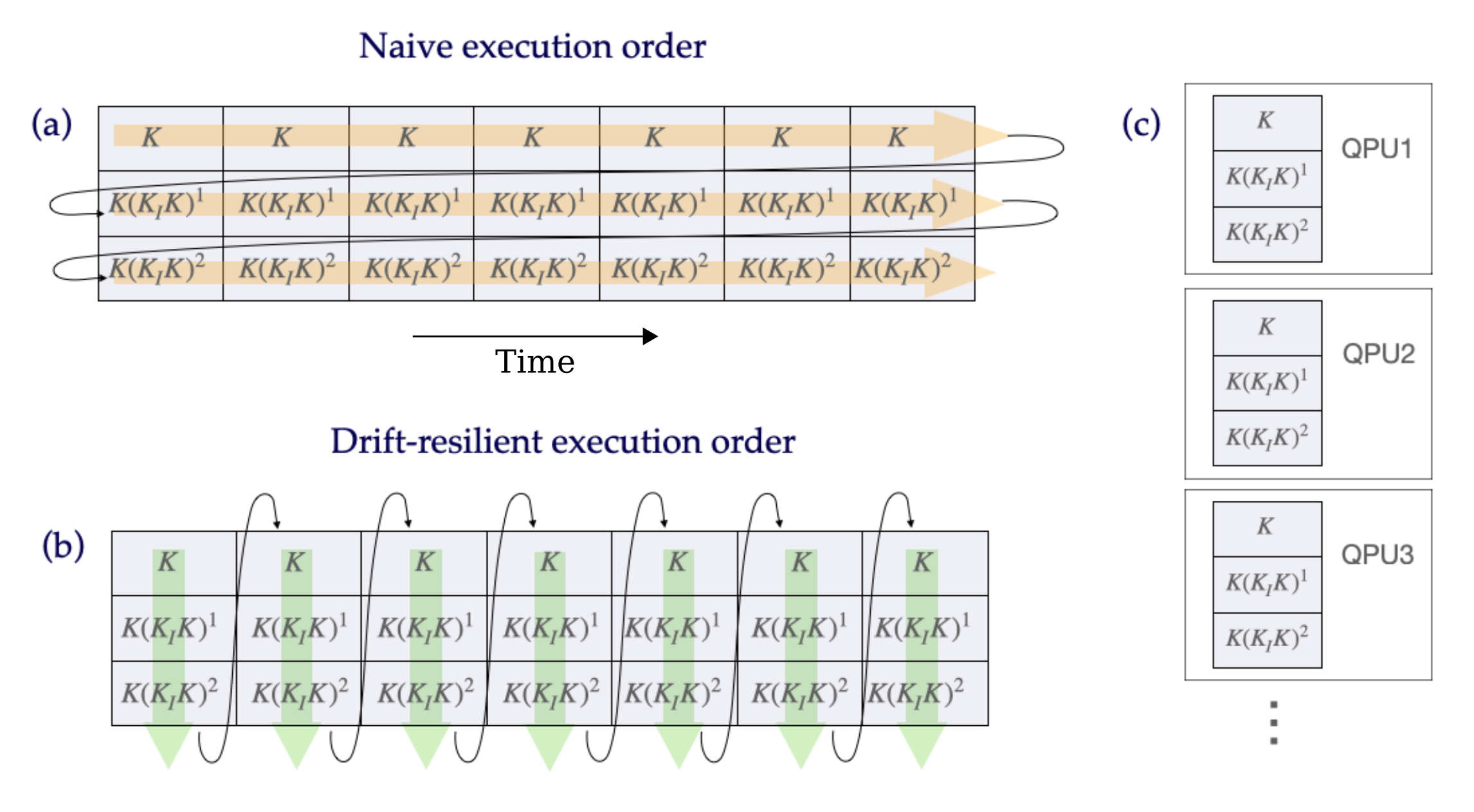
Supplementary Figure 2: Two strategies to collect data for second-order error mitigation, using the KIK method. The arrows indicate the order of implementation of different circuits. In (a), the implementations (shots) are separated into repetitions of each circuit $\mathcal{K}\left(\mathcal{K}_{\textrm{I}}\mathcal{K}\right)^{m}$, for $0\leq m\leq 2$ (horizontal groups). In (b), the shots are divided into $S$ sets (vertical groups) that include implementations of all the circuits $\mathcal{K}\left(\mathcal{K}_{\textrm{I}}\mathcal{K}\right)^{m}$. (a) and (b) depict circuit distributions with respect to time, for addressing noise drifts. The temporal sequence of circuit sets shown in (b) is rearranged as a “spatial distribution”, where different sets are implemented in different Quantum Processing Units (QPUs). This is useful for a parallel implementation of the KIK method.

Let us now suppose that noise unavoidably drifts in the interval $(0,t_{N})$. In this scenario, the consistency of the evolutions $\mathcal{K}$ or $\mathcal{K}_{\textrm{I}}$ in different shots can break down and prevent a correct implementation of the KIK formula (15). However, we can avoid or at least alleviate this effect through a proper distribution of the shot budget $N$. Consider Supplementary Figure 2, where two strategies for implementing the circuits $\{\mathcal{K}\left(\mathcal{K}_{\textrm{I}}\mathcal{K}\right)^{m}\}_{m=0}^{2}$ (second-order mitigation) are illustrated. In the case of Supplementary Figure 2(a), all the shots corresponding to a given $N_{m}$ are sequentially implemented, i.e., $N_{0}$ shots are first performed, followed by $N_{1}$ shots, and finally by $N_{2}$ shots. On the other hand, the strategy of Supplementary Figure 2(b) relies on dividing the $N$ shots into $S$ sets $\{n_{0},n_{1},n_{2}\}$ of $N_{S}=n_{0}+n_{1}+n_{2}$ shots each, where $n_{m}$ shots are employed for the circuit $\mathcal{K}\left(\mathcal{K}_{\textrm{I}}\mathcal{K}\right)^{m}$. Therefore, all the mitigation circuits $\mathcal{K}\left(\mathcal{K}_{\textrm{I}}\mathcal{K}\right)^{m}$ appear in each set. Without loss of generality for our argumentation, we can focus on the simple case where $n_{m}=N_{S}/3$ for $0\leq m\leq 2$, i.e. when the shots of each set are equally distributed into the different circuits $\mathcal{K}\left(\mathcal{K}_{\textrm{I}}\mathcal{K}\right)^{m}$.

Since each set $\{n_{0},n_{1},n_{2}\}$ contains data produced by all the circuits $\mathcal{K}\left(\mathcal{K}_{\textrm{I}}\mathcal{K}\right)^{m}$, the KIK formula can be individually applied to these data sets. Let

$$\mathcal{U}_{\textrm{KIK},s}=\mathcal{K}_{s}\left(\mathcal{K}_{\textrm{I};s}\mathcal{K}_{s}\right)^{-\frac{1}{2}}$$ (38)

denote the KIK formula corresponding to evolutions $\mathcal{K}_{s}$ and $\mathcal{K}_{\textrm{I},s}$ that are executed in shots of the $s$th set $\{n_{0},n_{1},n_{2}\}^{(s)}$. If there were no noise drifts, $\mathcal{K}_{s}=\mathcal{K}_{1}=\mathcal{K}$ and $\mathcal{K}_{\textrm{I};s}=\mathcal{K}_{\textrm{I};1}=\mathcal{K}_{\textrm{I}}$ for $1\leq s\leq S$. Therefore, the two strategies depicted in Supplementary Figure 2 would lead to the same result. Nevertheless, the non-stationary character of the noise may cause that $\mathcal{K}_{s}$ or $\mathcal{K}_{\textrm{I};s}$ change significantly when moving between different sets $\{n_{0},n_{1},n_{2}\}^{(s)}$, or even within a fixed set. The second possibility is less likely though, if the time $\sum_{m=0}^{M}n_{m}(2m+1)T$ invested in implementing each set $\{n_{0},n_{1},n_{2}\}^{(s)}$ is smaller than the characteristic time for noise drifts to be significant. In other words, if the time scale over which noise drifts occur is sufficiently large to allow a consistent execution of $\mathcal{U}_{\textrm{KIK},s}$. Assuming that $N_{S}$ is sufficiently small (equivalently, $S$ sufficiently large) for this to happen, for any $1\leq s\leq S$ we can implement the formula (38) without worrying about variations in the evolutions $\mathcal{K}_{s}$ or $\mathcal{K}_{\textrm{I};s}$. In this way, for the shot budget $N$ we utilize the “average KIK formula”

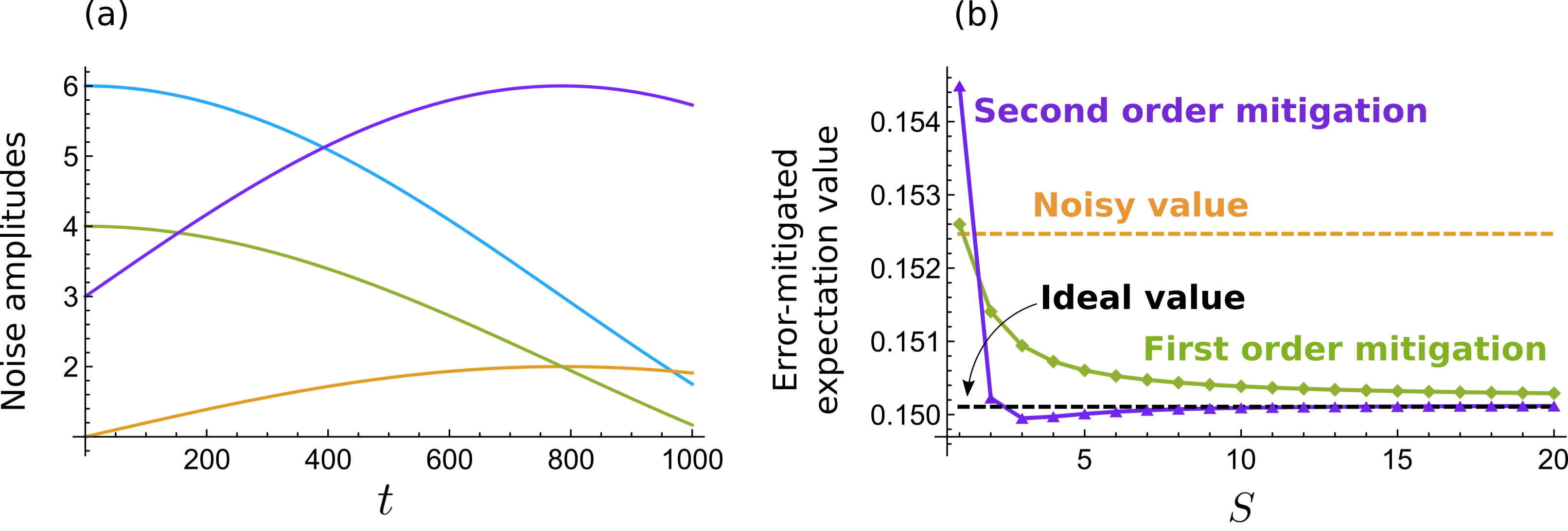
Supplementary Figure 3: KIK method applied to a system with noise drifts. (a) The four time-dependent amplitudes $f_{k}(t)$ that appear in the dissipator (40), and characterize the drift in noise parameters. (b) First order mitigation and second order mitigation using the average formula (39), as a function of the number of sets $S$ (see Supplementary Figure 2 and main text for details).

$$\mathcal{U}_{\textrm{KIK},\textrm{av}}^{(M)}=\frac{1}{S}\sum_{s=1}^{S}\mathcal{U}_{\textrm{KIK},s}^{(M)}.$$ (39)

A pertinent question when executing a computation is whether it can be parallelized and save time. The parallelization can be carried out using subsets of qubits in the same quantum processing unit (QPU), in a different QPU on the same chip, or on a different platform in a remote location. In the context of QEM, a recent proposal is to integrate this approach with virtual distillation ^{11; 12} techniques ⁴⁹.

The KIK method can easily be parallelized by assigning different sets to different QPUs as shown in Supplementary Figure 2(c). In this case, the index $s$ in Eq. (38) would label different QPUs, rather than different instants of time, and the corresponding error-mitigated expectation value would also be computed using (39). The justification is the same as in the case of noise drifts discussed above.

Let us now illustrate the application of this methodology to KIK mitigation under noise drifts. In Supplementary Figure 3, we consider two qubits subjected to a dissipator

$$\tilde{\mathcal{L}}(t)=\xi\sum_{k=1}^{4}f_{k}(t)\mathcal{L}_{k},$$ (40)

where $\xi=0.05$,

$$\mathcal{L}_{k} =A_{k}\otimes A_{k}^{\ast}-\frac{1}{2}A_{k}^{\dagger}A_{k}\otimes I-\frac{1}{2}I\otimes\left(A_{k}^{\dagger}A_{k}\right)^{\textrm{T}},$$ (41)

$$A_{1} =\left(\begin{array}[]{cc}0&1\\ 0&0\end{array}\right)\otimes\left(\begin{array}[]{cc}1&0\\ 0&1\end{array}\right),$$ (46)

$$A_{2} =\left(\begin{array}[]{cc}1&0\\ 0&0\end{array}\right)\otimes\left(\begin{array}[]{cc}1&0\\ 0&1\end{array}\right),$$ (51)

$$A_{3} =\left(\begin{array}[]{cc}1&0\\ 0&1\end{array}\right)\otimes\left(\begin{array}[]{cc}0&1\\ 0&0\end{array}\right),$$ (56)

$$A_{4} =\left(\begin{array}[]{cc}1&0\\ 0&1\end{array}\right)\otimes\left(\begin{array}[]{cc}1&0\\ 0&0\end{array}\right),$$ (61)

and

$$f_{1}(t) =3\left(1+\textrm{cos}(2t/T)\right),$$ (62)

$$f_{2}(t) =1+\textrm{sin}(2t/T),$$ (63)

$$f_{3}(t) =2\left(1+\textrm{cos}(2t/T)\right),$$ (64)

$$f_{4}(t) =3\left(1+\textrm{sin}(2t/T)\right).$$ (65)

The noise amplitudes $f_{k}(t)$ are plotted in Supplementary Figure 3(a), for $1\leq t\leq 1000$. Moreover, we assume a time-independent Hamiltonian (cf. Eq. (9))

$$\mathcal{H} =H\otimes I-I\otimes H^{\textrm{T}},$$ (66)

$$H =3X\otimes X+I\otimes X,$$ (67)

where $I=\left(\begin{array}[]{cc}1&0\\ 0&1\end{array}\right)$ and $X=\left(\begin{array}[]{cc}0&1\\ 1&0\end{array}\right)$.

$\tilde{\mathcal{L}}(t)$ is the Liouville-space representation of the Hilbert space dissipator that satisfies $\hat{L}(t)[\rho]=\xi\sum_{k=1}^{4}f_{k}(t)\hat{L}_{k}$, which follows by applying the vectorization rule (5) to each term $\hat{L}_{k}[\rho]=A_{k}\rho A_{k}^{\dagger}-\frac{1}{2}A_{k}^{\dagger}A_{k}\rho-\frac{1}{2}\rho A_{k}^{\dagger}A_{k}$. Since the associated master equation

$$\frac{d}{dt}|\rho\rangle=\left(-i\mathcal{H}+\tilde{\mathcal{L}}(t)\right)|\rho\rangle$$ (68)

has GKSL (Gorini–Kossakowski–Sudarshan–Lindblad) form, it is guaranteed that its integration results in a completely positive and trace-preserving evolution. We also stress that $\tilde{\mathcal{L}}(t)$ is now defined in the total time interval $(0,t_{N})$, to account for the many repetitions of the pulses $\mathcal{H}(t)$ and $\mathcal{H}_{\textrm{I}}(t-T)$ that come with the $N$ shots.

We numerically simulate QEM using the average formula (39), by setting

$$N =1000,$$ (69)

$$N_{S} =N/S,$$ (70)

$$n_{1} =n_{2}=n_{3}=N_{S}/3,$$ (71)

and $1\leq S\leq 20$. An execution of $\mathcal{K}$ or $\mathcal{K}_{\textrm{I}}$ is performed in a unit of time $T=1$, for which we assume that noise is essentially time independent. In other words, a more precise description of the noise occurring during the $N$ shots is given by the discrete dissipator

$$\tilde{\mathcal{L}}_{\textrm{disc}}(t)=\tilde{\mathcal{L}}(n),\textrm{ if }n\leq t\leq n+1,$$ (72)

with $\tilde{\mathcal{L}}(t)$ satisfying Eq. (40) and $0\leq n\leq N-1$.

Supplementary Figure 3(b) shows the error-mitigated expectation value $\left\langle\rho\right\rangle_{\textrm{mit}}=\left\langle\rho\left|\mathcal{U}_{\textrm{KIK},\textrm{av}}^{(M)}\right|\rho\right\rangle$, which quantifies the overlap with the initial state $\rho=I/2\otimes|0\rangle\langle 0|$. We apply Taylor error mitigation, using the coefficients $a_{\textrm{Tay},m}^{(M)}$ given in Eq. (77). If $S=1$, the standard strategy represented in Supplementary Figure 2(a) is recovered. We observe in Supplementary Figure 3(b) that in this case $\left\langle\rho\right\rangle_{\textrm{mit}}$ deviates drastically from the noiseless expectation value $\left\langle\rho\right\rangle_{\textrm{id}}=\left\langle\rho\left|\mathcal{U}\right|\rho\right\rangle$. As $S$ increases, second-order mitigation quickly approaches $\left\langle\rho\right\rangle_{\textrm{id}}$ and converges to it at $S\approx 10$. We also stress that for $S\geq 10$ the quality of error mitigation is maintained, both for $M=1$ and $M=2$, which shows that averaging the KIK formula over more sets does not degrade the performance of the KIK method. The success of this strategy is explained because $\left\langle\rho\right\rangle_{\textrm{mit}}=\frac{1}{S}\sum_{s=1}^{S}\left\langle\rho\left|\mathcal{U}_{\textrm{KIK},s}^{(M)}\right|\rho\right\rangle$, and if noise is approximately stationary for each $\mathcal{U}_{\textrm{KIK},s}^{(M)}$ then the corresponding $\left\langle\rho\left|\mathcal{U}_{\textrm{KIK},s}^{(M)}\right|\rho\right\rangle$ is not affected by the action of noise drifts. However, the number of shots $N_{S}$ associated with each set is not sufficiently large to achieve the accuracy shown in Supplementary Figure 3(b). This accuracy is achieved after averaging over the total number of sets. The convergence observed in Supplementary Figure 3(b) confirms that in this example increasing the number of sets enhances the QEM performance, and solves the noise drift problem.

Supplementary Note 4: Implementations of the inverse of the noise channel $\mathcal{N}_{\textrm{KIK}}$

The KIK formula (15) provides a compact approximation for the ideal target evolution $\mathcal{U}$. However, performing QEM with this formula also requires being able to physically implement the inverse

$$\mathcal{N}_{\textrm{KIK}}^{-1}=\left(\mathcal{K}_{\textrm{I}}\mathcal{K}\right)^{-\frac{1}{2}}.$$ (73)

In this section, we compute various approximations to this inverse, given as polynomials of the KIK cycle $\mathcal{K}_{\textrm{I}}\mathcal{K}$.

Weak noise limit and Taylor approximation. First, we consider the limit of weak noise. As mentioned in the main text, in this case any eigenvalue $\lambda$ of $\mathcal{K}_{\textrm{I}}\mathcal{K}$ is close to 1, and we can obtain the eigenvalues of $\left(\mathcal{K}_{\textrm{I}}\mathcal{K}\right)^{-\frac{1}{2}}$ by Taylor expanding $\lambda^{-\frac{1}{2}}$ around $\lambda=1$. Note that here we assume that noise is such that $\mathcal{K}_{\textrm{I}}\mathcal{K}$ is still diagonalizable, and therefore the eigenvalues of $\left(\mathcal{K}_{\textrm{I}}\mathcal{K}\right)^{-\frac{1}{2}}$ can be obtained as $\lambda^{-\frac{1}{2}}$.

A Taylor expansion of $\lambda^{-\frac{1}{2}}$ around $\lambda=1$ is thus equivalent to expand $\left(\mathcal{K}_{\textrm{I}}\mathcal{K}\right)^{-\frac{1}{2}}$ around the identity $\mathcal{I}$. Namely,

$$\left(\mathcal{K}_{\textrm{I}}\mathcal{K}\right)^{-\frac{1}{2}} =\sum_{m=0}^{\infty}c_{m}\left(\mathcal{K}_{\textrm{I}}\mathcal{K}-\mathcal{I}\right)^{m}$$

$$=\sum_{m=0}^{\infty}c_{m}\sum_{k=0}^{m}\frac{m!(-1)^{m-k}}{k!(m-k)!}\left(\mathcal{K}_{\textrm{I}}\mathcal{K}\right)^{k},$$ (74)

where

$$c_{m}=\frac{1}{m!}\frac{d^{m}\lambda^{-\frac{1}{2}}}{d\lambda^{m}}\left|{}_{\lambda=1}\right.=\left(-1\right)^{m}\frac{(2m-1)!!}{m!2^{m}}.$$ (75)

Since the series (74) involves infinite powers of $\mathcal{K}_{\textrm{I}}\mathcal{K}$, we must truncate it to some fixed order $M$ for the implementation of $\left(\mathcal{K}_{\textrm{I}}\mathcal{K}\right)^{-\frac{1}{2}}$. In this way,

$$\left(\mathcal{K}_{\textrm{I}}\mathcal{K}\right)^{-\frac{1}{2}} \approx\sum_{m=0}^{M}c_{m}\sum_{k=0}^{m}\frac{m!(-1)^{m-k}}{k!(m-k)!}\left(\mathcal{K}_{\textrm{I}}\mathcal{K}\right)^{k}$$

$$=\sum_{m=0}^{M}a_{\textrm{Tay},m}^{(M)}\left(\mathcal{K}_{\textrm{I}}\mathcal{K}\right)^{m},$$ (76)

where

$$a_{\textrm{Tay},m}^{(M)}=(-1)^{m}\frac{(2M+1)!!}{2^{M}[(2m+1)m!(M-m)!]}.$$ (77)

Richardson ZNE using Circuit folding and linear scaling of noise. In the following, we show that the expansion coefficients (77) predict the result of QEM using Richardson ZNE and noise amplification through a method known as circuit folding ¹³, under the assumption of a linear scaling of the noise. To put this result into context, we start by presenting the basics of Richardson ZNE and circuit folding.

The goal of ZNE is to infer the noise-free expectation value of an observable $A$, by measuring this observable at different levels of noise and then extrapolating to the zero-noise limit. Therefore, the application of ZNE requires assuming a certain functional dependence $\langle A\rangle(\lambda)$, between the expectation value $\langle A\rangle$ and some noise parameter $\lambda$ over which the experimentalist should have control. By measuring expectation values $\langle A\rangle_{k}$ corresponding to different levels of noise $\lambda_{k}$, an experimentalist can fit the data $[\lambda_{k},\langle A\rangle_{k}]$ to the model $\langle A\rangle(\lambda)$ and thereby estimate the noiseless expectation value as $\langle A\rangle(0)$. In the case of Richardson extrapolation, for $M+1$ data points $[\lambda_{k},\langle A\rangle_{k}]$, $\langle A\rangle(\lambda)$ is taken as a polynomial in $\lambda$ of degree $M$.

There exists a unique polynomial $P(\lambda)$ of degree $M$ that intersects all the points $[\lambda_{k},\langle A\rangle_{k}]$. This polynomial can be constructed as $P(\lambda)=\sum_{m=0}^{M}\langle A\rangle_{m}l_{m}(\lambda)$, where

$$l_{m}(\lambda):=\prod_{0\leq k\leq M,k\neq m}\frac{\lambda-\lambda_{k}}{\lambda_{m}-\lambda_{k}}$$ (78)

is a Lagrange polynomial of degree $M$. Noting that $l_{m}(\lambda_{k})=\delta_{km},$ it follows that $P(\lambda_{k})=\langle A\rangle_{k}$ for $0\leq k\leq M$. Therefore, the noise-free expectation value is estimated by

$$\langle A\rangle(0) =P(0)$$

$$=\sum_{m=0}^{M}\langle A\rangle_{m}l_{m}(0)$$

$$=\sum_{m=0}^{M}\langle A\rangle_{m}\prod_{0\leq k\leq M,k\neq m}\frac{\lambda_{k}}{\lambda_{k}-\lambda_{m}}.$$ (79)

Equation (79) gives $\langle A\rangle(0)$ in terms of $\langle A\rangle_{k}$ and the noise strengths $\lambda_{k}$. One of the first techniques proposed to artificially increase the value of $\lambda$ is pulse stretching ⁶, which involves pulse control from the user. In addition, we point out that pulse stretching also assumes that the noise is time-independent. Unitary folding is an alternative that does not require this level of control. If $\mathcal{U}$ describes the target ideal evolution, unitary folding operates by adding quantum gates to $\mathcal{U}$ that in the noise-free case are just identity operations. This can be done either by using “circuit foldings” $\mathcal{U}^{\dagger}\mathcal{U}$, or by inserting products between gates and their own inverses. Noting that the polynomial (76) contains powers of the (noisy) implementation of ${\normalcolor\mathcal{U}^{\dagger}\mathcal{U}}$, we are specifically interested in the connection between this polynomial and the use of circuit folding for ZNE, rather than folding at the level of gates. In this context, the assumption of linear scaling of the noise means that each power $\left(\mathcal{K}_{\textrm{I}}\mathcal{K}\right)^{k}$ increases the noise characteristic of $\mathcal{K}$ by a factor of $2k$, i.e. that the noise increases proportionally to the depth of the circuit $\left(\mathcal{K}_{\textrm{I}}\mathcal{K}\right)^{k}$. If $\lambda_{0}$ corresponds to the natural noise in the target circuit $\mathcal{K}$, then, the folding $\mathcal{K}\left(\mathcal{K}_{\textrm{I}}\mathcal{K}\right)^{k}$ results in $\lambda_{k}=(2k+1)\lambda_{0}$. By substituting this expression of $\lambda_{k}$ into $\prod_{0\leq k\leq M,k\neq m}\frac{\lambda_{k}}{\lambda_{k}-\lambda_{m}}$, we obtain:

$$\prod_{0\leq k\leq M,k\neq m}\frac{\lambda_{k}}{\lambda_{k}-\lambda_{m}} =\prod_{0\leq k\leq M,k\neq m}\frac{2k+1}{2(k-m)}$$

$$=\frac{\prod_{0\leq k\leq M,k\neq m}(2k+1)}{2^{M}\prod_{0\leq k\leq M,k\neq m}(k-m)}$$

$$=\frac{(2M+1)!!/(2m+1)}{2^{M}[(-m)(1-m)...(-1)][(1)(2)...(M-m)]}$$

$$=(-1)^{m}\frac{(2M+1)!!}{2^{M}[(2m+1)m!(M-m)!]},$$ (80)

which coincides with the coefficient $a_{\textrm{Tay},m}^{(M)}$ [cf. Eq. (77)].

Taking into account that $\langle A\rangle_{m}=\langle A|\mathcal{K}\left(\mathcal{K}_{\textrm{I}}\mathcal{K}\right)^{m}|\rho\rangle$, it follows that the application of the KIK formula in the weak noise limit reproduces the prediction of Richardson ZNE, with circuit folding and linear scaling of noise [cf. Eqs. (79) and (80)]. As a final remark, it is worth noting that in circuit folding the realization of $\mathcal{U}^{\dagger}$ using circuit level of control does not involve modifying gates that are their own inverse. A fundamental example in this respect is the CNOT gate, which is the basic unit of two-qubit interactions. In contrast, the pulse inverse $\mathcal{H}_{\textrm{I}}(t)$ used in our method reverses also the schedules of the CNOT gates, to keep consistency with the pulse-based inverse $\mathcal{K}_{\textrm{I}}$ appearing in the KIK formula (15).

In what follows, we also show that using $\mathcal{K}=\mathcal{K}_{\textrm{I}}$ in the case of target circuits that are their own inverse introduces an additional error term that is absent when $\mathcal{K}_{\textrm{I}}$ is the pulse inverse. This further demonstrates the importance of the correct implementation of $\mathcal{K}_{\textrm{I}}$ for KIK QEM.

Error induced by the circuit inverse $\mathcal{K}_{\textrm{I}}=\mathcal{K}$ in circuits that satisfy $\mathcal{U}^{2}=\mathcal{I}$. Previously, we showed that the coefficients $a_{\textrm{Tay},m}^{(M)}$ reproduce Richardson ZNE when noise is linearly scaled through circuit folding. However, even in this limit of weak noise the KIK method provides insights that elude a naive application of circuit folding. An example of this was already given in Supplementary Note 3, by showing that, even though $\mathcal{K}\mathcal{K}_{\textrm{I}}$ and$\mathcal{K}_{\textrm{I}}\mathcal{K}$ are equivalent in the noiseless scenario, the product $\mathcal{K}_{\textrm{I}}\mathcal{K}$ is the correct choice for using the KIK formula (15). This is valid in particular for Eq. (76).

Here, we will see that ignoring the pulse inverse $\mathcal{K}_{\textrm{I}}$ also has negative consequences for QEM using Eq. (76), which for simplicity we call “Taylor mitigation”. Specifically, we consider circuits such that

$$\mathcal{U}^{2}=\mathcal{I},$$ (81)

which suggests the application of (76) with $\mathcal{K}_{\textrm{I}}=\mathcal{K}$. In this way, the $M$th order approximation to $\mathcal{U}$ (cf. Eq. (2) in the main text) reads

$$\mathcal{U}_{\textrm{KIK}}^{(M)} =\sum_{m=0}^{M}a_{\textrm{Tay},m}^{(M)}\mathcal{K}\left(\mathcal{K}\mathcal{K}\right)^{m}$$

$$=\sum_{m=0}^{M}a_{\textrm{Tay},m}^{(M)}\left(\mathcal{K}\right)^{2m+1}$$

$$=\sum_{m=0}^{M}a_{\textrm{Tay},m}^{(M)}\left(\mathcal{U}e^{\Omega_{1}}\right)^{2m+1},$$ (82)

where $\mathcal{K}$ has been replaced by Eq. (23) and $\Omega_{1}=\Omega_{1}(T)$.

Next, we approximate $\mathcal{U}e^{\Omega_{1}}$ by $\mathcal{U}e^{\Omega_{1}}\approx\mathcal{U}+\mathcal{U}\Omega_{1}$, and keep only terms that are linear in $\Omega_{1}$ in $\mathcal{U}_{\textrm{KIK}}^{(M)}$. Using $\mathcal{U}^{2m+1}=\mathcal{U}$, we have that

$$\left(\mathcal{U}+\mathcal{U}\Omega_{1}\right)^{2m+1}\approx\mathcal{U}+\sum_{k=1}^{2m+1}\mathcal{U}^{k}\Omega_{1}\mathcal{U}^{2m+1-k},$$ (83)

for $m\geq 1$. Therefore,

$$\mathcal{U}_{\textrm{KIK}}^{(M)} \approx a_{\textrm{Tay},0}^{(M)}\left(\mathcal{U}+\mathcal{U}\Omega_{1}\right)+\sum_{m=1}^{M}a_{\textrm{Tay},m}^{(M)}\left(\mathcal{U}e^{\Omega_{1}}\right)^{2m+1}$$

$$\approx a_{\textrm{Tay},0}^{(M)}\left(\mathcal{U}+\mathcal{U}\Omega_{1}\right)+\sum_{m=1}^{M}a_{\textrm{Tay},m}^{(M)}\left[\mathcal{U}+\sum_{k=1}^{2m+1}\mathcal{U}^{k}\Omega_{1}\mathcal{U}^{2m+1-k}\right]$$

$$=\mathcal{U}+a_{\textrm{Tay},0}^{(M)}\mathcal{U}\Omega_{1}+\sum_{m=1}^{M}a_{\textrm{Tay},m}^{(M)}\sum_{k=1}^{2m+1}\mathcal{U}^{k}\Omega_{1}\mathcal{U}^{2m+1-k},$$ (84)

where we have applied $\sum_{m=0}^{M}a_{\textrm{Tay},m}^{(M)}=1$.

Now we divide the sum $\sum_{k=1}^{2m+1}\mathcal{U}^{k}\Omega_{1}\mathcal{U}^{2m+1-k}$ into two sums such that one of them contains only even powers $\mathcal{U}^{k}$, and the other contains only odd powers $\mathcal{U}^{k}$. Taking into account that $\mathcal{U}^{-1}=\mathcal{U}$ and that any even power of $\mathcal{U}$ yields $\mathcal{I}$, we obtain

$$\sum_{k=1}^{2m+1}\mathcal{U}^{k}\Omega_{1}\mathcal{U}^{2m+1-k} =\sum_{k=1}^{m+1}\mathcal{U}^{2k-1}\Omega_{1}\mathcal{U}^{2m+2-2k}+\sum_{k=1}^{m}\mathcal{U}^{2k}\Omega_{1}\mathcal{U}^{2m+1-2k}$$

$$=\sum_{k=1}^{m+1}\mathcal{U}\Omega_{1}+\sum_{k=1}^{m}\Omega_{1}\mathcal{U}$$

$$=(m+1)\mathcal{U}\Omega_{1}+m\Omega_{1}\mathcal{U}.$$ (85)

Substituting Eq. (85) into Eq. (84), we find that

$$\mathcal{U}_{\textrm{KIK}}^{(M)} \approx\mathcal{U}+a_{\textrm{Tay},0}^{(M)}\mathcal{U}\Omega_{1}+\sum_{m=1}^{M}a_{\textrm{Tay},m}^{(M)}\left[(m+1)\mathcal{U}\Omega_{1}+m\Omega_{1}\mathcal{U}\right]$$

$$=\mathcal{U}+a_{\textrm{{Tay},0}}^{(M)}\mathcal{U}\Omega_{1}+\sum_{m=0}^{M}a_{\textrm{Tay},m}^{(M)}\left[(m+1)\mathcal{U}\Omega_{1}+m\Omega_{1}\mathcal{U}\right]-a_{\textrm{Tay},0}^{(M)}\mathcal{U}\Omega_{1}$$

$$=\mathcal{U}+\sum_{m=0}^{M}a_{\textrm{Tay},m}^{(M)}\left[(m+1)\mathcal{U}\Omega_{1}+m\Omega_{1}\mathcal{U}\right],$$ (86)

where in the second line we added and subtracted the term corresponding to $m=0$ in the sum.

Finally, we use again $\sum_{m=0}^{M}a_{\textrm{Tay},m}^{(M)}=1$, and $\sum_{m=0}^{M}a_{\textrm{Tay},m}^{(M)}m=-\frac{1}{2}$. In this way, for any $M\geq 1$,

$$\mathcal{U}_{\textrm{KIK}}^{(M)}\approx\mathcal{U}+\frac{1}{2}[\mathcal{U},\Omega_{1}].$$ (87)

Because Taylor mitigation corresponds to weak noise, in the limit when $M$ tends to infinity $\mathcal{U}_{\textrm{KIK}}^{(M)}$ should converge to the evolution $\mathcal{U}_{\textrm{KIK}}$ in the KIK formula (15). By construction, this is the case if $\mathcal{K}_{\textrm{I}}$ is given by the pulse inverse. However, we see from Eq. (87) that when $\mathcal{K}_{\textrm{I}}=\mathcal{K}$ the term $\frac{1}{2}[\mathcal{U},\Omega_{1}]$ remains in the approximation $\mathcal{U}_{\textrm{KIK}}^{(M)}$, irrespective of the mitigation order $M$. Note also that this term cannot be avoided in general by considering higher-order (nonlinear) contributions in $\Omega_{1}$. In this way, Eq. (87) shows that using $\mathcal{K}_{\textrm{I}}=\mathcal{K}$ instead of the pulse inverse leads to an inconsistent application of QEM, which is afflicted by an additional error term $\frac{1}{2}[\mathcal{U},\Omega_{1}]$.

Finally, we remark that for global depolarizing noise the associated noise channel commutes with any unitary $\mathcal{U}$, and one can easily check that in this case the KIK formula (15) is exact when $\mathcal{K}_{\textrm{I}}=\mathcal{K}$. Thus, while the pulse-based inverse $\mathcal{K}_{\textrm{I}}$ becomes unnecessary for such a simplified noise model ¹³, it is of paramount importance in practical applications under realistic noise.

Coefficients for Adaptive QEM based on the KIK formula, for mitigation orders $M=1,2,3$. To obtain the coefficients $a_{\textrm{Adap},m}^{(M)}$, we minimize the quantity

$$\varepsilon_{\textrm{L2}}^{(M)}:=\int_{g(\mu)}^{1}\left(\sum_{m=0}^{M}a_{m}^{(M)}\lambda^{m}-\lambda^{-\frac{1}{2}}\right)^{2}d\lambda$$ (88)

with respect the first $M$ coefficients $\left\{a_{m}^{(M)}\right\}_{m=0}^{M-1}$. Therefore, we have to solve the equations

$$\frac{\partial\varepsilon_{\textrm{L2}}^{(M)}}{\partial a_{m}^{(M)}}=0,\quad\textrm{for }0\leq m\leq M-1.$$ (89)

The $M$th coefficient is obtained by imposing the constraint $a_{\textrm{Adap},M}^{(M)}=1-\sum_{m=0}^{M-1}a_{\textrm{Adap},m}^{(M)}$. This is equivalent to the normalization condition $\sum_{m=0}^{M}a_{\textrm{Adap},m}^{(M)}=1$, which ensures that the map ${\normalcolor{\color[rgb]{1,0,0}{\normalcolor\mathcal{U}_{\textrm{KIK}}^{(M)}=}}}\sum_{m=0}^{M}a_{\textrm{Adap},m}^{(M)}[g(\mu)]\mathcal{K}\left(\mathcal{K}_{\textrm{I}}\mathcal{K}\right)^{m}$ is trace-preserving if $\mathcal{K}$ and $\mathcal{K}_{\textrm{I}}$ are trace-preserving. For the sake of notational simplicity, in the following we will write $g(\mu)$ as $g$.

By explicitly evaluating $\varepsilon_{\textrm{L2}}^{(M)}$ with $M=1,2,3$, we find that

$$\varepsilon_{\textrm{L2}}^{(1)}=(1-g)\left(a_{0}^{(1)}\right)^{2}+\frac{1}{3}(1-g^{3})\left(a_{1}^{(1)}\right)^{2}+(1-g^{2})a_{0}^{(1)}a_{1}^{(1)}-4(1-g^{\frac{1}{2}})a_{0}^{(1)}-\frac{4}{3}(1-g^{\frac{3}{2}})a_{1}^{(1)}-\textrm{ln}(g),$$ (90)

$$\varepsilon_{\textrm{L2}}^{(2)} =(1-g)\left(a_{0}^{(2)}\right)^{2}+\frac{1}{3}(1-g^{3})\left(a_{1}^{(2)}\right)^{2}+\frac{1}{5}(1-g^{5})\left(a_{2}^{(2)}\right)^{2}+(1-g^{2})a_{0}^{(2)}a_{1}^{(2)}+\frac{2}{3}(1-g^{3})a_{0}^{(2)}a_{2}^{(2)}$$

$$\quad+\frac{1}{2}(1-g^{4})a_{1}^{(2)}a_{2}^{(2)}-4(1-g^{\frac{1}{2}})a_{0}^{(2)}-\frac{4}{3}(1-g^{\frac{3}{2}})a_{1}^{(2)}-\frac{4}{5}(1-g^{\frac{5}{2}})a_{2}^{(2)}-\textrm{ln}(g),$$ (91)

$$\varepsilon_{\textrm{L2}}^{(3)} =(1-g)\left(a_{0}^{(3)}\right)^{2}+\frac{1}{3}(1-g^{3})\left(a_{1}^{(3)}\right)^{2}+\frac{1}{5}(1-g^{5})\left(a_{2}^{(3)}\right)^{2}+\frac{1}{7}(1-g^{7})\left(a_{3}^{(3)}\right)^{2}$$

$$\quad+(1-g^{2})a_{0}^{(3)}a_{1}^{(3)}+\frac{2}{3}(1-g^{3})a_{0}^{(3)}a_{2}^{(3)}+\frac{1}{2}(1-g^{4})a_{0}^{(3)}a_{3}^{(3)}+\frac{1}{2}(1-g^{4})a_{1}^{(3)}a_{2}^{(3)}+\frac{2}{5}(1-g^{5})a_{1}^{(3)}a_{3}^{(3)}$$

$$\quad+\frac{1}{3}(1-g^{6})a_{2}^{(3)}a_{3}^{(3)}-4(1-g^{\frac{1}{2}})a_{0}^{(3)}-\frac{4}{3}(1-g^{\frac{3}{2}})a_{1}^{(3)}-\frac{4}{5}(1-g^{\frac{5}{2}})a_{2}^{(3)}-\frac{4}{7}(1-g^{\frac{7}{2}})a_{3}^{(3)}-\textrm{ln}(g).$$ (92)

By taking the partial derivatives (89) and solving the resulting linear equations, the corresponding coefficients read

$$a_{\textrm{Adap},0}^{(1)} =1+\frac{1}{(1+\sqrt{g})^{3}}+\frac{3}{2(1+\sqrt{g})^{2}},$$ (93)

$$a_{\textrm{Adap},1}^{(1)} =-\frac{5+3\sqrt{g}}{2(1+\sqrt{g})^{3}},$$ (94)

for $M=1,$

$$a_{\textrm{Adap},0}^{(2)} =1+\frac{16}{3(1+\sqrt{g})^{5}}-\frac{14}{3(1+\sqrt{g})^{4}}+\frac{4}{(1+\sqrt{g})^{2}},$$ (95)

$$a_{\textrm{Adap},1}^{(2)} =-4\frac{10+8\sqrt{g}+9g+3g^{\frac{3}{2}}}{3(1+\sqrt{g})^{5}},$$ (96)

$$a_{\textrm{Adap},2}^{(2)} =2\frac{13+5\sqrt{g}}{3(1+\sqrt{g})^{5}},$$ (97)

for $M=2,$ and

$$a_{\textrm{Adap},0}^{(3)} =\frac{31+97\sqrt{g}+276g+300g^{\frac{3}{2}}+270g^{2}+114g^{\frac{5}{2}}+28g^{3}+4g^{\frac{7}{2}}}{4(1+\sqrt{g})^{7}},$$ (98)

$$a_{\textrm{Adap},1}^{(3)} =-5\frac{29+35\sqrt{g}+84g+44g^{\frac{3}{2}}+26g^{2}+6g^{\frac{5}{2}}}{4(1+\sqrt{g})^{7}},$$ (99)

$$a_{\textrm{Adap},2}^{(3)} =3\frac{81+47\sqrt{g}+76g+20g^{\frac{3}{2}}}{4(1+\sqrt{g})^{7}},$$ (100)

$$a_{\textrm{Adap},3}^{(3)} =-5\frac{25+7\sqrt{g}}{4(1+\sqrt{g})^{7}},$$ (101)

for $M=3$.

Let us now check that the obtained coefficients minimize $\varepsilon_{\textrm{L2}}^{(M)}$ in the subspace determined by the variables $\left\{a_{m}^{(M)}\right\}_{m=0}^{M-1}$. For $M=1$, the second derivative $\frac{\partial^{2}\varepsilon_{\textrm{L2}}^{(1)}}{\partial a_{0}^{(1)2}}=2\left(1-g\right)$ is positive if $g\leq 1$, and therefore $a_{\textrm{Adap},0}^{(1)}$ minimizes $\varepsilon_{\textrm{L2}}^{(1)}$ with respect to $a_{0}^{(1)}$. To see if $a_{\textrm{Adap},0}^{(2)}$ and $a_{\textrm{Adap},1}^{(2)}$ in Eqs. (93) and (94) minimize $\varepsilon_{\textrm{L2}}^{(2)}$, we evaluate the determinant of the Hessian matrix of $\varepsilon_{\textrm{L2}}^{(2)}$ and the second partial derivative $\frac{\partial^{2}\varepsilon_{\textrm{L2}}^{(2)}}{\partial a_{0}^{(2)2}}$, and check their positivity. Since $\frac{\partial^{2}\varepsilon_{\textrm{L2}}^{(2)}}{\partial a_{0}^{(2)2}}=2(1-g)\geq 0$, we only need to check the determinant of the Hessian matrix

$$H=\left(\begin{array}[]{cc}\frac{\partial^{2}\varepsilon_{\textrm{L2}}^{(2)}}{\partial a_{0}^{(2)2}}&\frac{\partial^{2}\varepsilon_{\textrm{L2}}^{(2)}}{\partial a_{0}^{(2)}\partial a_{1}^{(2)}}\\ \frac{\partial^{2}\varepsilon_{\textrm{L2}}^{(2)}}{\partial a_{1}^{(2)}\partial a_{0}^{(2)}}&\frac{\partial^{2}\varepsilon_{\textrm{L2}}^{(2)}}{\partial a_{1}^{(2)2}}\end{array}\right)=\left(\begin{array}[]{cc}2\left(1-g\right)&1-g^{2}\\ 1-g^{2}&\frac{2}{3}(1-g^{3})\end{array}\right).$$ (102)

Such a determinant is given by $\textrm{det}(H)=\frac{4}{3}\left[1-g\right]\left[1-g^{3}\right]-\left[1-g^{2}\right]^{2}$, which is also positive in the interval $0\leq g\leq 1$. Finally, for $M=3$ we obtain the Hessian matrix

$$H=\left(\begin{array}[]{ccc}\frac{\partial^{2}\varepsilon_{\textrm{L2}}^{(3)}}{\partial a_{0}^{(3)2}}&\frac{\partial^{2}\varepsilon_{\textrm{L2}}^{(3)}}{\partial a_{0}^{(3)}\partial a_{1}^{(3)}}&\frac{\partial^{2}\varepsilon_{\textrm{L2}}^{(3)}}{\partial a_{0}^{(3)}\partial a_{2}^{(3)}}\\ \frac{\partial^{2}\varepsilon_{\textrm{L2}}^{(3)}}{\partial a_{1}^{(3)}\partial a_{0}^{(3)}}&\frac{\partial^{2}\varepsilon_{\textrm{L2}}^{(3)}}{\partial a_{1}^{(3)2}}&\frac{\partial^{2}\varepsilon_{\textrm{L2}}^{(3)}}{\partial a_{1}^{(3)}\partial a_{2}^{(3)}}\\ \frac{\partial^{2}\varepsilon_{\textrm{L2}}^{(3)}}{\partial a_{2}^{(3)}\partial a_{0}^{(3)}}&\frac{\partial^{2}\varepsilon_{\textrm{L2}}^{(3)}}{\partial a_{2}^{(3)}\partial a_{1}^{(3)}}&\frac{\partial^{2}\varepsilon_{\textrm{L2}}^{(3)}}{\partial a_{2}^{(3)2}}\end{array}\right)=\left(\begin{array}[]{ccc}2(1-g)&1-g^{2}&\frac{2}{3}(1-g^{3})\\ 1-g^{2}&\frac{2}{3}(1-g^{3})&\frac{1}{2}(1-g^{4})\\ \frac{2}{3}(1-g^{3})&\frac{1}{2}(1-g^{4})&\frac{2}{5}(1-g^{5})\end{array}\right).$$ (103)

The eigenvalues of this matrix are plotted in Supplementary Figure 4. Since all of them are positive in the interval $0\leq g\leq 1$, we conclude that Eqs. (98)-(101) provide the coefficients $a_{\textrm{Adap},m}^{(3)}$ that minimize $\varepsilon_{\textrm{L2}}^{(3)}$ with respect to $\left\{a_{m}^{(M)}\right\}_{m=0}^{2}$.

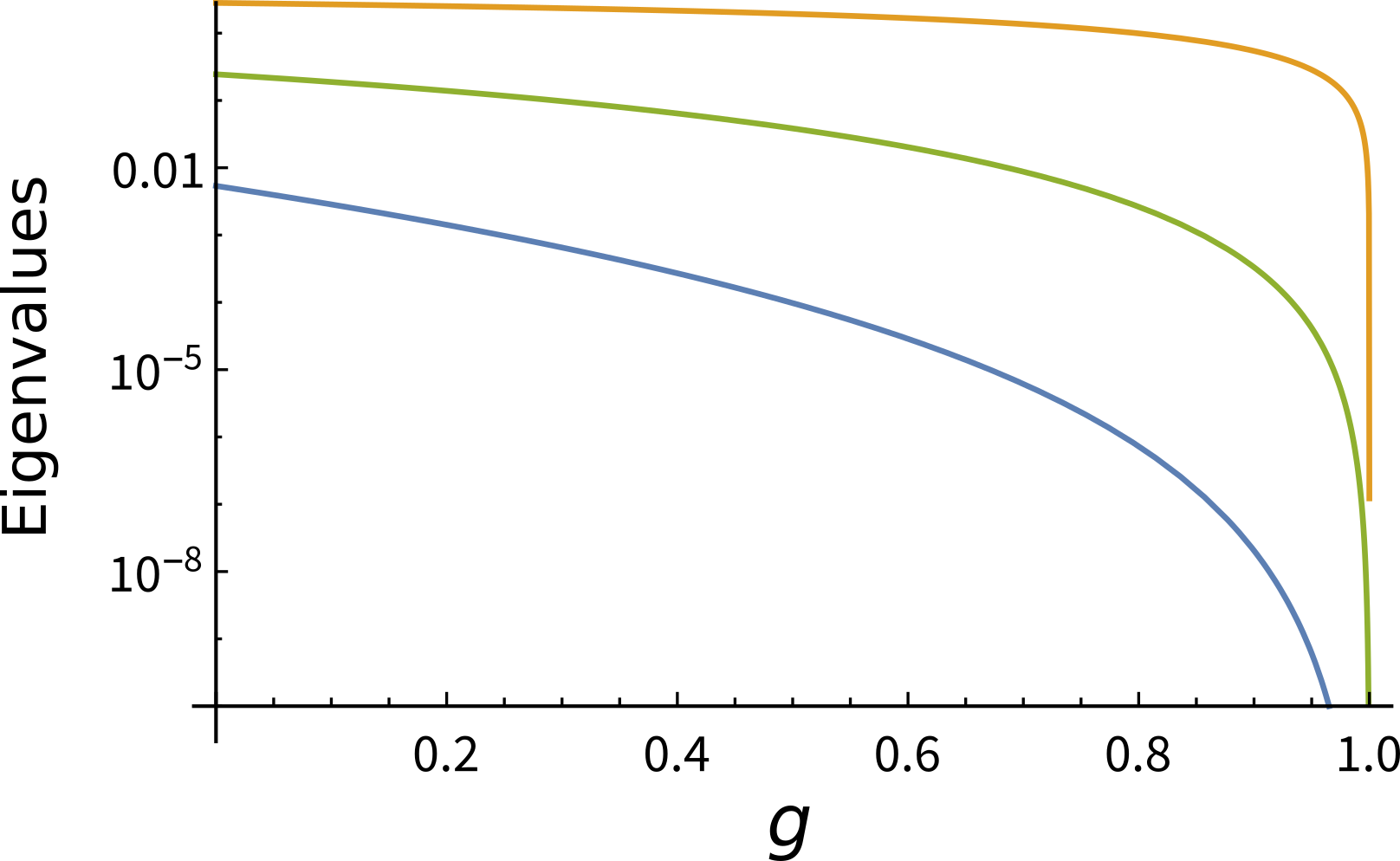
Supplementary Figure 4: Eigenvalues of the Hessian matrix (103), as a function of $g=g(\mu)$.

Supplementary Note 5: KIK QEM applied to the transverse Ising model

In this supplementary note, we simulate the application of the KIK method to a noisy implementation of the transverse Ising model. This model is characterized by the Hamiltonian

$$H =g\sum_{i=1}^{n}X_{i}+J\sum_{i=1}^{n-1}Z_{i}\otimes Z_{i+1}$$

$$:=gH_{X}+JH_{ZZ}$$ (104)

where $H_{ZZ}$ accounts for the magnetic interactions between nearest-neighbor spins, and the transverse magnetic fields are represented by the local term $H_{X}$. We consider $n=5$ spins and set $g=0.2$ and $J=0.1$. There is no particular reason for choosing these parameter values. Similar performance was obtained with simulations using alternative values (not shown here).

For the simulation, we assume that the target evolution $U=e^{-iHT}$ is implemented in a quantum computer via Trotterization ³⁸. Taking into account that the $X$ and $Z$ Pauli matrices do not commute, an approximation to $U$ involving $n$ Trotter steps has the form

$$U\approx U_{n}:=\left(e^{-igH_{X}\frac{T}{n}}e^{-iJH_{ZZ}\frac{T}{n}}\right)^{n},$$ (105)

where $T$ is the total evolution time. Assuming $T=10$ and 10 Trotter steps, we have that

$$U \approx U_{10}$$

$$:=\left(e^{-igH_{X}}e^{-iJH_{ZZ}}\right)^{10}.$$ (106)

In what follows, $I_{j}$ will denote the identity matrix of dimension $2^{j}\times 2^{j}$, with $I=I_{n}$. We remark that our goal is not to test the accuracy of the Trotter approximation (106), but to study the performance of the KIK method to mitigate errors in a noisy implementation of $U_{10}$. To this end, we model the noisy evolution $\mathcal{K}$ associated with $U_{10}$ using

$$\mathcal{K} =\left(e^{-ig\mathcal{H}_{X}+\xi\mathcal{L}}e^{-iJ\mathcal{H}_{ZZ}+\xi\mathcal{L}}\right)^{10},$$ (107)

$$\mathcal{H}_{X} =H_{X}\otimes I-I\otimes\left(H_{X}\right)^{\textrm{T}},$$ (108)

$$\mathcal{H}_{ZZ} =H_{ZZ}\otimes I-I\otimes\left(H_{ZZ}\right)^{\textrm{T}},$$ (109)

where

$$\mathcal{{\normalcolor L}} {\normalcolor=S\otimes S^{\ast}-\frac{1}{2}S^{\dagger}S\otimes I-\frac{1}{2}I\otimes\left(S^{\dagger}S\right)^{\textrm{T}},}$$ (110)

$$S =0.5S_{1}+1.7S_{2}+0.3S_{3}+2S_{4}+S_{5},$$ (111)

$$S_{j} ={\color[rgb]{1,0,0}{\normalcolor I_{j-1}}}\otimes A\otimes{\color[rgb]{1,0,0}{\normalcolor I_{n-j}}},\textrm{ for }1\leq j\leq 5,$$ (112)

$$A {\color[rgb]{0,0,1}{\normalcolor=\left(\begin{array}[]{cc}0&1\\ 0&0\end{array}\right)}.}$$ (115)

The initial state in our simulation is the ground state $\rho=|0\rangle\langle 0|^{\otimes 5}$.

Error mitigation. To assess the performance of the KIK QEM, we use the fidelity between

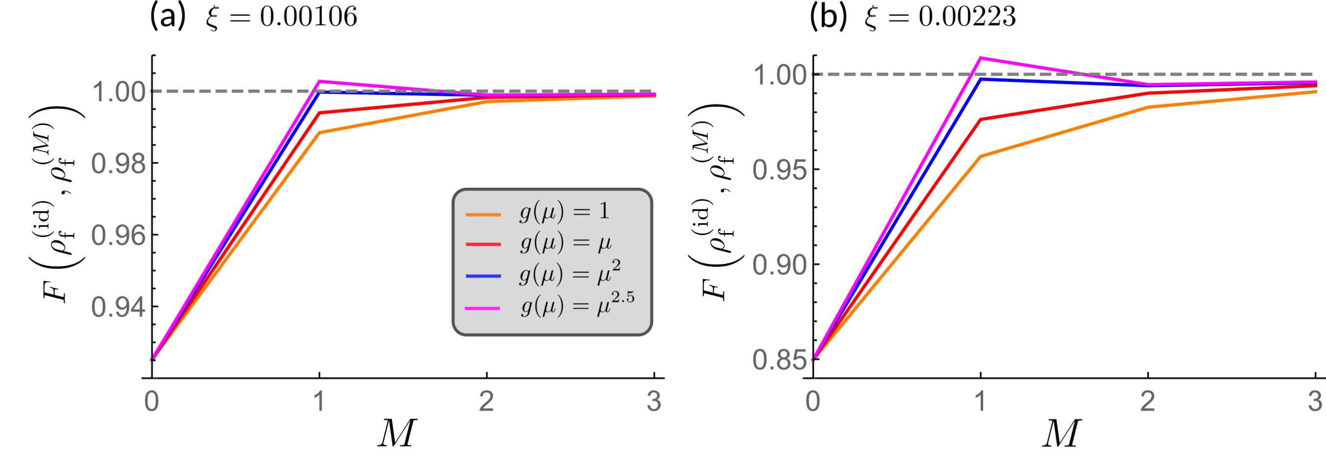
Supplementary Figure 5: Error-mitigated fidelity $F\left(\rho_{\textrm{f}}^{(\textrm{id})},\rho_{\textrm{f}}^{(M)}\right)$, between the ideal final state $|\rho_{\textrm{f}}^{(\textrm{id})}\rangle=\mathcal{U}_{10}|\rho\rangle$ and the error-mitigated final state $|\rho_{\textrm{f}}^{(M)}\rangle:=\mathcal{U}_{\textrm{KIK}}^{(M)}|\rho\rangle$. Each curve is obtained by evaluating the coefficients $a_{\textrm{Adap},m}^{(M)}[g(\mu)]$ in the $M$th-order approximation ${\normalcolor{\color[rgb]{1,0,0}{\normalcolor\mathcal{U}_{\textrm{KIK}}^{(M)}=}}}\sum_{m=0}^{M}a_{\textrm{Adap},m}^{(M)}[g(\mu)]\mathcal{K}\left(\mathcal{K}_{\textrm{I}}\mathcal{K}\right)^{m}$ at the functions $g(\mu)$ indicated in Supplementary Figure 5(a). Supplementary Figures 5(a) and 5(b) stand respectively for $\xi=0.00106$ and $\xi=0.00223$, and both are characterized by the color code of Supplementary Figure 5(a).

the ideal final state $|\rho_{\textrm{f}}^{(\textrm{id})}\rangle:=\mathcal{U}_{10}|\rho\rangle$ (being $\mathcal{U}_{10}$ the Liouville-space representation of $U_{10}$) and the error-mitigated final state $|\rho_{\textrm{f}}^{(M)}\rangle:=\mathcal{U}_{\textrm{KIK}}^{(M)}|\rho\rangle$, which reads ⁵⁰

$$F\left(\rho_{\textrm{f}}^{(\textrm{id})},\rho_{\textrm{f}}^{(M)}\right)=\left[\textrm{Tr}\sqrt{\sqrt{\rho_{\textrm{f}}^{(\textrm{id})}}\rho_{\textrm{f}}^{(M)}\sqrt{\rho_{\textrm{f}}^{(\textrm{id})}}}\right]^{2}.$$ (116)

Notice that the fidelity must be computed using the density matrices $\rho_{\textrm{f}}^{(\textrm{id})}$ and $\rho_{\textrm{f}}^{(M)}$, and not their vector representations $|\rho_{\textrm{f}}^{(\textrm{id})}\rangle$ and $|\rho_{\textrm{f}}^{(M)}\rangle$. We consider values of $\xi$ given by $\xi=0.00223$ and $\xi=0.00106$, which lead to fidelities of unmitigated final states ($M=0$)

$$F\left(\rho_{\textrm{f}}^{(\textrm{id})},\rho_{\textrm{f}}^{(0)}\right) =0.85,\textrm{ for }\xi=0.00223,$$ (117)

$$F\left(\rho_{\textrm{f}}^{(\textrm{id})},\rho_{\textrm{f}}^{(0)}\right) =0.925,\textrm{ for }\xi=0.00106.$$ (118)

QEM is performed by choosing functions $\{g(\mu)\}=\{1,\mu,\mu^{2},\mu^{2.5}\}$, and $1\leq M\leq 3$. We recall that the function $g(\mu)$ determines the lower limit of integration in $\varepsilon_{\textrm{L2}}^{(M)}$ (see the main text for the definition), and that for each $g(\mu)$ QEM is applied with ${\normalcolor{\color[rgb]{1,0,0}{\normalcolor\mathcal{U}_{\textrm{KIK}}^{(M)}=}}}\sum_{m=0}^{M}a_{\textrm{Adap},m}^{(M)}[g(\mu)]\mathcal{K}\left(\mathcal{K}_{\textrm{I}}\mathcal{K}\right)^{m}$, using coefficients $a_{\textrm{Adap},m}^{(M)}[g(\mu)]$ evaluated at $g=g(\mu)$ (cf. Supplementary Note 4). In particular, $g(\mu)=1$ corresponds to Taylor mitigation. Keeping in mind Eq. (107), the inverse $\mathcal{K}_{\textrm{I}}$ is given by

$$\mathcal{K}_{\textrm{I}}=\left(e^{iJ\mathcal{H}_{ZZ}+\xi\mathcal{L}}e^{ig\mathcal{H}_{X}+\xi\mathcal{L}}\right)^{10}.$$ (119)

Supplementary Figure 5 shows the fidelity $F\left(\rho_{\textrm{f}}^{(\textrm{id})},\rho_{\textrm{f}}^{(M)}\right)$ as a function of $M$, for $\xi=0.00106$ and $\xi=0.00223$. Overall, we observe that the best performance among the tested functions $g(\mu)$ is achieved by $g(\mu)=\mu^{2}$ (blue curve). In particular, $F\left(\rho_{\textrm{f}}^{(\textrm{id})},\rho_{\textrm{f}}^{(M)}\right)$ reaches a value extremely close to one already for $M=1$. A clearer comparison between the different functions $g(\mu)$ is possible by looking at the ratio between the infidelity before QEM and after QEM,

$$r_{F}(M)=\frac{1-F\left(\rho_{\textrm{f}}^{(\textrm{id})},\rho_{\textrm{f}}^{(0)}\right)}{1-F\left(\rho_{\textrm{f}}^{(\textrm{id})},\rho_{\textrm{f}}^{(M)}\right)},$$ (120)

which quantifies the infidelity suppression provided by the KIK method. This quantity is plotted in Supplementary Figure 6. In this figure, we see that $g(\mu)=\mu^{2}$ outperforms $g(\mu)=1$ and $g(\mu)=\mu$ for all $1\leq M\leq 3$. Although the ratio $r_{F}(M)$ corresponding to $g(\mu)=\mu^{2}$ is slightly below that associated with $g(\mu)=\mu^{2.5}$, in the case of $M=2,3$, $g(\mu)=\mu^{2}$ yields a substantially larger $r_{F}(M)$ if $M=1$.

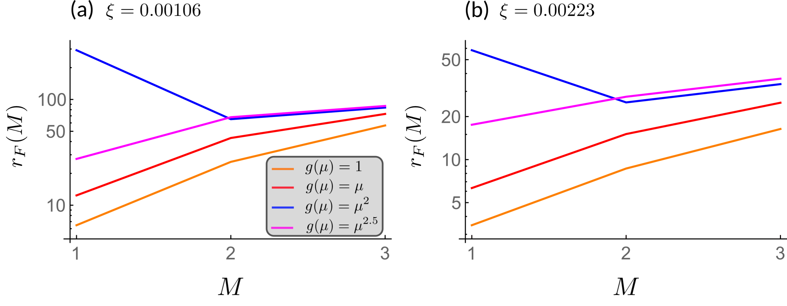
Supplementary Figure 6: Enhancement ratio (120), which quantifies the infidelity suppression obtained by the KIK method. The color code in Supplementary Figure 6(b) is the same as in 6(a).

Finally, it is interesting to observe how the different functions $g(\mu)$ produce physically consistent fidelities $F\left(\rho_{\textrm{f}}^{(\textrm{id})},\rho_{\textrm{f}}^{(M)}\right)\leq 1$ as $M$ increases. In particular, we can see that the unphysical fidelity $F\left(\rho_{\textrm{f}}^{(\textrm{id})},\rho_{\textrm{f}}^{(1)}\right)>1$ corresponding to $g(\mu)=\mu^{2.5}$ is quickly fixed by going to the next mitigation order $M=2$. The explanation for this behavior is as follows. The quality of the approximation $\sum_{m=0}^{M}a_{\textrm{Adap},m}^{(M)}[g(\mu)]\left(\mathcal{K}_{\textrm{I}}\mathcal{K}\right)^{m}$ to $\left(\mathcal{K}_{\textrm{I}}\mathcal{K}\right)^{-1/2}$ is determined by how well the polynomial $\sum_{m=0}^{M}a_{\textrm{Adap},m}^{(M)}[g(\mu)]\lambda^{m}$ approximates the function $\lambda^{-1/2}$, where $\lambda$ is an eigenvalue of $\mathcal{K}_{\textrm{I}}\mathcal{K}$. If $g(\mu)$ is too small, as compared to the smallest eigenvalue of $\left(\mathcal{K}_{\textrm{I}}\mathcal{K}\right)^{-1/2}$, a polynomial $\sum_{m=0}^{M}a_{\textrm{Adap},m}^{(M)}[g(\mu)]\left(\mathcal{K}_{\textrm{I}}\mathcal{K}\right)^{m}$ with low $M$ may be a rough approximation to $\left(\mathcal{K}_{\textrm{I}}\mathcal{K}\right)^{-1/2}$. This leads to undesired effects such as the aforementioned fidelity $F\left(\rho_{\textrm{f}}^{(\textrm{id})},\rho_{\textrm{f}}^{(1)}\right)>1$ (note that in our example the function $g(\mu)=\mu^{2.5}$ yields the smallest $g(\mu)$ for any value of $\mu$). However, by increasing $M$ we can always improve the approximation in the whole interval $(g(\mu),1)$, which by assumption contains all the eigenvalues of $\left(\mathcal{K}_{\textrm{I}}\mathcal{K}\right)^{-1/2}$. This would explain not only the recovery of a physical fidelity but also that for $M=2$ and $M=3$ the maximum values of this quantity correspond to $g(\mu)=\mu^{2.5}$.

On the contrary, when $g(\mu)$ is larger than the smallest eigenvalue of $\left(\mathcal{K}_{\textrm{I}}\mathcal{K}\right)^{-1/2}$, the interval $(g(\mu),1)$ does not contain all the eigenvalues of $\left(\mathcal{K}_{\textrm{I}}\mathcal{K}\right)^{-1/2}$ and increasing $M$ does not necessarily improves the QEM. This is likely the reason that $g(\mu)=\mu^{2}$ yields fidelities smaller for $M=2$ and $M=3$, as compared to $M=1$.

Supplementary Note 6: Description of the experimental procedures

Here, we provide additional details and complementary information concerning the experiments described in the main text. In the first subsection we describe techniques to tackle different classes of errors, which complement the KIK error mitigation. Next, we explain in detail the steps to estimate error-mitigated expectation values, as well as the corresponding uncertainties. Then, information specific to the CNOT calibration experiment and the ten-swap experiment is given in the following two subsections. We conclude in the last subsection with a simulated calibration of the CNOT gate. This simulation shows results very similar to those of the CNOT calibration experiment, and provides additional evidence of the usefulness of KIK-based calibration.

Integration with complementary error mitigation methods. We consider three complementary techniques for addressing errors that can affect an experiment in the three stages of its execution. Namely, the preparation of the initial state, the evolution, and the measurement.

In the IBM quantum processors the preparation of the single-qubit (default) computational state $|0\rangle$ may possess a small deviation angle $\delta\theta$ ⁴⁴. As a result, the prepared state is given by $|\psi(\delta\theta)\rangle=\textrm{cos}\left(\frac{\delta\theta}{2}\right)|0\rangle+e^{i\varphi}\textrm{sin}\left(\frac{\delta\theta}{2}\right)|1\rangle$. To cope with this error, we apply rotations $R_{Z}(\pm\pi/2)=e^{\mp i\frac{\pi}{4}Z}$ on each qubit, in such a way that $R_{Z}(\pi/2)$ and $R_{Z}(-\pi/2)$ are equally distributed among the number of shots. This produces a mixed state

$$\varrho=\textrm{cos}^{2}\left(\frac{\delta\theta}{2}\right)|0\rangle\langle 0|+\textrm{sin}^{2}\left(\frac{\delta\theta}{2}\right)|1\rangle\langle 1|,$$ (121)

whose population $\textrm{Tr}\left(|0\rangle\langle 0|\varrho\right)=\textrm{cos}^{2}\left(\frac{\delta\theta}{2}\right)$ coincides with $|\langle 0|\psi(\delta\theta)\rangle|^{2}$. However, the coherent error associated with the rotation angles $\delta\theta$ and $\varphi$ is eliminated through this procedure. Since both experiments involve circuits acting on two qubits, there are four possible rotation operations characterized by the pairs of angles $\{(\pm\pi/2,\pm\pi/2)\}$. This is illustrated by the green squares in Supplementary Figure 7(a).

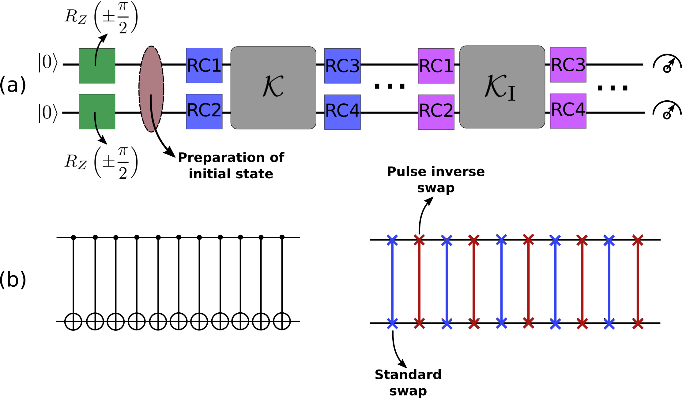
Supplementary Figure 7: Schematic of the QEM circuits used in the experiments. (a) General form of a KIK circuit $\mathcal{K}\left(\mathcal{K}_{\textrm{I}}\mathcal{K}\right)^{m}$. For both experiments, initial rotations $R_{Z}(\pm\pi/2)$ (green squares) are applied on each qubit to mitigate a potential coherent error affecting the state $|00\rangle$. After that, the initial state for the CNOT calibration experiment is prepared (this preparation is not part of the ten-swap experiment), and the evolutions $\mathcal{K}$ and $\mathcal{K}_{\textrm{I}}$ are interleaved by RC operations (only in the case of the ten-swap experiment). Blue and magenta squares distinguish potentially different RC realizations, chosen from Supplementary Table 1. (b) The evolution $\mathcal{K}$ used for the CNOT calibration experiment (left), and for the ten-swap experiment (right).

Coherent errors present during the evolution stage of a quantum circuit can be specially harmful for quantum computing ⁵¹. Randomized compiling (RC) ³² is a standard method that allows to transform these errors into stochastic noise, which is amenable to the application of QEM using the KIK method. The essential idea of RC is to replace the target circuit by an average over compiled realizations that are logically equivalent to the original evolution. Each RC realization is obtained by randomly replacing and/or adding some gates that leave the noise-free target circuit invariant. However, in the presence of coherent errors, different RC realizations produce different evolutions, and coherent errors characteristic of single realizations can be averaged out into stochastic noise.

In our method, the implementation $\mathcal{U}_{\textrm{KIK}}^{(M)}$ of the KIK formula contains both the target evolution $\mathcal{K}$ and its inverse $\mathcal{K}_{\textrm{I}}$. Therefore, for each KIK power $\mathcal{K}\left(\mathcal{K}_{\textrm{I}}\mathcal{K}\right)^{m}$ we independently applied RC on $\mathcal{K}$ and $\mathcal{K}_{\textrm{I}}$, as indicated in Supplementary Figure 7(a). This is done by using the Pauli gates shown in Supplementary Table 1, which are performed before and after the execution of $\mathcal{K}$ and $\mathcal{K}_{\textrm{I}}$ in the ten-swap experiment. A sequence of ten swap gates is logically equivalent to the identity operation, and one can straightforwardly check that each RC realization in Supplementary Table 1 reproduces this operation. Furthermore, we remark that an independent application of RC on $\mathcal{K}$ and $\mathcal{K}_{\textrm{I}}$ is important to perform an effective randomization of the coherent errors affecting both evolutions. This ensures that the first Magnus terms appearing in the evolutions $\mathcal{K}$ and $\mathcal{K}_{\textrm{I}}\mathcal{K}$ (cf. Eqs. (23) and (24)) are still related through Eq. (25), and thus validates the KIK formula with the randomized versions of $\mathcal{K}$ and $\mathcal{K}_{\textrm{I}}$. Along the same line, we avoid the simplification of RC layers in any sequence $\mathcal{K}\left(\mathcal{K}_{\textrm{I}}\mathcal{K}\right)^{m}$. This means that consecutive single-qubit gates used for RC are not merged into a single gate. Otherwise, the independence of the randomization would be affected by preventing that the gates of the original pair act separately on $\mathcal{K}$ and $\mathcal{K}_{\textrm{I}}$.

On the other hand, for the CNOT calibration experiment we omitted the use of RC. The reason is that, in this experiment, we explored an alternative mitigation of coherent errors affecting the calibrated gate, which operates differently from RC. More specifically, a KIK-based mitigation of stochastic noise in the calibration process can improve the quality of the calibration, which translates into a calibrated gate with reduced coherent errors.

RC1	RC2
$I$	$I$
$I$	$X$
$I$	$Y$
$I$	$Z$

RC1	RC2
$X$	$I$
$X$	$X$
$X$	$Y$
$X$	$Z$

RC1	RC2
$Y$	$I$
$Y$	$X$
$Y$	$Y$
$Y$	$Z$

RC1	RC2
$Z$	$I$
$Z$	$X$
$Z$	$Y$
$Z$	$Z$

Supplementary Table 1: Possible combinations of RC operations used for the evolutions $\mathcal{K}$ and $\mathcal{K}_{\textrm{I}}$ in the ten-swap experiment. Here, RC1 and RC2 stand for Pauli gates that are performed as indicated in Supplementary Figure 7(a). Since in this circuit the ideal unitary associated with $\mathcal{K}$ and $\mathcal{K}_{\textrm{I}}$ is the identity, the gate RC3 must coincide with RC1, and the gate RC4 must coincide with RC2.

A final ingredient for our QEM experiments is the mitigation of readout errors. For a circuit executed on $N$ qubits, the measurement process outputs counts of the states $|i_{1}i_{2}...i_{N}\rangle$ ($i_{j}\in\{0,1\}$ for $1\leq j\leq N$) in the computational basis. A readout error occurs when the state registered upon the measurement is incorrect. For example, for a single qubit whose final state is $|1\rangle$, some counts may erroneously register the state as being $|0\rangle$.

Let us denote a general $N$-bit string by $\bm{k}=(k_{1}k_{2}...k_{N})$, and the corresponding computational state by $|\bm{k}\rangle$. When a quantum circuit produces a final state $\sigma$, readout errors cause wrong estimates of the probabilities $p_{\bm{k}}=\textrm{Tr}\left(|\bm{k}\rangle\langle\bm{k}|\sigma\right)$. A simple way to relate the ideal probabilities $p_{\bm{k}}$ and the erroneous ones is by considering the probability distributions associated with each computational state. If $p\left(\bm{l}|\bm{k}\right)$ denotes the conditional probability to register the state $|\bm{l}\rangle$, given that the actual state is $|\bm{k}\rangle$, for the final state $\sigma$ the probability to measure $|\bm{l}\rangle$ in the presence of readout errors is given by

$$q_{\bm{l}}=\sum_{\bm{k}}p\left(\bm{l}|\bm{k}\right)p_{\bm{k}}.$$ (122)

Thus, the information about the readout errors is contained in a $2^{N}\times 2^{N}$ matrix $\mathbf{M}$ with entries $p\left(\bm{l}|\bm{k}\right)$, whose columns and rows are associated with $\bm{k}$ and $\bm{l}$, respectively. To counteract the effect of the readout errors, we can invert the “measurement matrix” $\mathbf{M}$. In this way, the vector of error-free probabilities can be obtained by applying the inverse $\mathbf{M}^{-1}$ to the vector of measured probabilities.

Although the procedure described above is not scalable in $N$, because the size of $\mathbf{M}$ is exponential in the number of qubits, our experiments involve two qubits and admit an efficient estimation of the $p\left(\bm{l}|\bm{k}\right)$. To this end, we prepared the four computational states $\{|ij\rangle\}_{i,j=0}^{1}$ using circuits with the appropriate $X$ gates. For example, $|01\rangle$ is prepared by applying $X$ on the second qubit. The measurement matrices were experimentally determined and then inverted for readout error mitigation in both the CNOT calibration experiment and the ten-swap experiment. The number of shots invested in the estimation of the distributions $\{p\left(\bm{l}|\bm{k}\right)\}_{\bm{l}}$ is given in Supplementary Table 2.

As a final comment, it is important to mention that the study of methods to efficiently cope with readout errors in circuits containing a large number of qubits is an active area of research. For example, in many cases the noisy probability distribution $q_{\bm{l}}$ is mostly concentrated around the ideal distribution $p_{\bm{k}}$. This allows to construct a measurement matrix of reduced dimension that is defined over the subspace of bit strings with $q_{\bm{l}}\neq 0$ ¹⁷. In particular, the maximum size of such a matrix is determined by the maximum number of shots used to sample $q_{\bm{l}}$, and is independent of the number of qubits.

Statistical analysis of experimental data. The experimental estimates of different probability distributions are computed as frequencies over the number of shots. Ultimately, the goal is to estimate probability distributions $\{p_{\bm{k}}^{(m,i)}\}_{\bm{k}}$ for each $m$ and $i$, where $p_{\bm{k}}^{(m,i)}$ denotes the probability to measure $|\bm{k}\rangle$ when the circuit $\mathcal{K}\left(\mathcal{K}_{\textrm{I}}\mathcal{K}\right)^{m}$ is implemented in combination with the $i$th RC realization. These probabilities are the key element for the computation of expectation values and the application of QEM.

In the case of the ten-swap experiment, we applied 16 RC realizations of each circuit $\mathcal{K}\left(\mathcal{K}_{\textrm{I}}\mathcal{K}\right)^{m}$. Hence, for any $m$ the expectation value $\textrm{Tr}\left(O\sigma\right)$ of an observable $O$ is estimated as

$$\left\langle O\right\rangle_{m} =\frac{1}{N_{\textrm{RC}}}\sum_{i=1}^{N_{\textrm{RC}}}\left\langle O\right\rangle_{m,i},$$ (123)

$$\left\langle O\right\rangle_{m,i} =\sum_{\bm{k}}p_{\bm{k}}^{(m,i)}O_{\bm{k}},$$ (124)

where $N_{\textrm{RC}}=16$. Importantly, for observables that are not diagonal in the computational basis, the final state $\sigma$ in $\textrm{Tr}\left(O\sigma\right)$ must contain a rotation that performs the corresponding change of basis. For example, to measure the observable $O=Y_{1}$ on qubit 1, for the CNOT calibration experiment, before the measurement we applied a rotation $R_{X_{1}}(\pi/2)=e^{-i\frac{\pi}{4}X_{1}}$ on this qubit.

Since different RC realizations correspond to independent experiments, the variance for $\left\langle O\right\rangle_{m}$ reads

$$\textrm{Var}\left(\left\langle O\right\rangle_{m}\right) =\frac{1}{N_{\textrm{RC}}^{2}}\sum_{i=1}^{N_{\textrm{RC}}}\textrm{Var}\left(\left\langle O\right\rangle_{m,i}\right)$$

$$=\frac{1}{N_{\textrm{RC}}^{2}}\sum_{i=1}^{N_{\textrm{RC}}}\left[\frac{\sum_{\bm{k}}p_{\bm{k}}^{(m,i)}O_{\bm{k}}^{2}-\left\langle O\right\rangle_{m,i}^{2}}{N_{i}}\right],$$ (125)

where $N_{i}$ is the number of shots used in the $i$th RC realization. In the CNOT calibration experiment RC was not implemented, as mentioned before. However, Eqs. (123)-(125) are still applicable in this case, with $N_{\textrm{RC}}=8$ being the number of circuits associated with different initial rotations, and the index $i$ labeling any of these circuits.

The KIK method provides the error-mitigated expectation value

$$\left\langle O\right\rangle_{M}=\sum_{m=0}^{M}a_{m}^{(M)}\left\langle O\right\rangle_{m},$$ (126)

with the coefficients $a_{m}^{(M)}$ chosen depending on the QEM strategy. Namely, Taylor mitigation, or adaptive mitigation. The independence of the experiments associated with different circuits $\mathcal{K}\left(\mathcal{K}_{I}\mathcal{K}\right)^{m}$ leads to the variance

$$\textrm{Var}\left(\left\langle O\right\rangle_{M}\right)=\sum_{m=0}^{M}\left(a_{m}^{(M)}\right)^{2}\textrm{Var}\left(\left\langle O\right\rangle_{m}\right).$$ (127)

The error bars in the plots of the main text and the plots of Supplementary Figures 8 and 9 correspond to one standard deviation. That is, half of each error bar is given by $\sqrt{\textrm{Var}\left(\left\langle O\right\rangle_{M}\right)}$.

CNOT calibration experiment. The calibration experiment was performed on the IBM processor Jakarta, using the qubits labeled by 0 and 1. The qubit 0 was employed as control for the CNOT gate and the qubit 1 as target. In the IBM processors, the two-qubit interaction used to generate the CNOT gate is effectively implemented via the so called cross-resonance interaction ⁴⁵ $H_{\textrm{CR}}=Z\otimes X$, where $Z$ and $X$ are the Pauli matrices $Z=\left(\begin{array}[]{cc}1&0\\ 0&-1\end{array}\right)$ and $X=\left(\begin{array}[]{cc}0&1\\ 1&0\end{array}\right)$ acting on the control qubit and target qubit, respectively. The CNOT thus involves a $\pi/2$ rotation with the Hamiltonian $H_{\textrm{CR}}$. This operation is performed in the quantum processor by applying a microwave pulse characterized by various calibrated parameters such as amplitude and duration. However, the values obtained for these parameters may be affected by systematic errors, due to noise present in the measurements used for calibration.

We focus on the calibration of the pulse amplitude, using the KIK method to mitigate the effect of noise. As explained in the main text, we prepare the initial state $\frac{1}{\sqrt{2}}\left(|0\rangle+|1\rangle\right)\otimes|0\rangle$ and measure the observable $Y=\left(\begin{array}[]{cc}0&-i\\ i&0\end{array}\right)$ on the target qubit for different pulse amplitudes. This choice of initial state and observable is convenient because it produces a calibration curve that is very well described by a straight line. We measured the expectation value $\left\langle Y_{1}\right\rangle$ for the amplitude factors $F\in\{0.98,0.9866,0.9933,1,1.0066,1.0133,1.02\}$, where $F=1$ corresponds to the default amplitude used by IBM, and fitted a straight line to the resulting data points. The calibrated amplitude factor is extracted from the intersection of the fitted line with the $x$ axis, which corresponds to $\left\langle Y_{1}\right\rangle=0$. The range of amplitudes $F$ was chosen to be sufficiently narrow, so that one could observe the linear behavior previously described.

To increase the precision of the calibration, the experiment was performed using a sequence of 11 CNOT gates. Ideally, this circuit is equivalent to a single CNOT, and the repetition of CNOTs has the effect of amplifying the variations of $\left\langle Y_{1}\right\rangle$ associated with different values of $F$. Accordingly, the inverse $\mathcal{K}_{\textrm{I}}$ for the left circuit in Supplementary Figure 7(b) consists of a sequence of gates such that each of them is the pulse inverse of a single CNOT.

In the processor Jakarta, the maximum number of shots per circuit is 32000. For the mitigation of readout errors, we repeated four times the circuits employed in the preparation of each computational state, which yields a total of $4\times 32000=128000$ shots used to estimate each probability distribution $\{p\left(\bm{l}|\bm{k}\right)\}_{\bm{l}}$. The circuits $\mathcal{K}\left(\mathcal{K}_{\textrm{I}}\mathcal{K}\right)^{m}$, used for QEM, were preceded by any of the four rotation operations used to mitigate the preparation coherent error. These rotations were executed before the preparation of the initial state, as seen in Supplementary Figure 7(a). We repeated two times the circuit corresponding to any rotation. Hence, $8\times 32000=256000$ shots were employed to measure the expectation value of $Y_{1}$ on each $\mathcal{K}\left(\mathcal{K}_{\textrm{I}}\mathcal{K}\right)^{m}$, for each amplitude $F$. Since we applied KIK mitigation up to order 3, the value of $m$ varies between 0 and 3. These experimental details are summarized in Supplementary Table 2.

Ten-swap experiment. In this experiment,

	shots per KIK circuit	shots for readout mitigation	RC operations
CNOT calibration experiment	256000	512000	n/a
ten-swap experiment	320000	240000	16

Supplementary Table 2: Summary of experimental resources. The ‘shots per KIK circuit’ are the number of shots associated with each circuit ${\normalcolor\mathcal{K}\left(\mathcal{K}_{\textrm{I}}\mathcal{K}\right)^{m}}$, for $0\leq m\leq 3$. For both experiments, these shots include the initial rotations, and also RC operations in the case of the ten-swap experiment. The ‘shots for readout mitigation’ are the total number of shots used to compute $\mathbf{M}^{-1}$.

the error-mitigated quantity was the probability for the system to remain in the initial state $|00\rangle$, after applying a sequence of ten swap gates. The IBM processor employed was Quito. In practice, three CNOT gates were used to implement each swap, as shown in Fig. 4(b) of the main text. Apart from the application of RC, detailed below, we reduced the impact of coherent errors by alternating a normal swap with a pulse-based inverse swap (see Supplementary Figure 7(b)). This strategy has been previously applied to gates that are their own inverse, with the purpose of mitigating coherent errors such as overrotations ⁵². Since a swap gate is its own inverse, our ideal target circuit is not modified by interleaving standard swaps with their pulse-inverse counterparts.

Let us now describe in more detail the distribution of the different circuits for this experiment. As in the previous case, any of the circuits ${\normalcolor\mathcal{K}\left(\mathcal{K}_{\textrm{I}}\mathcal{K}\right)^{m}}$ was preceded by one of the four rotation operations applied on the state $|00\rangle$. For $0\leq m\leq 3$, a circuit ${\normalcolor\mathcal{K}\left(\mathcal{K}_{\textrm{I}}\mathcal{K}\right)^{m}}$ is accompanied by a rotation operation and a RC operation chosen at random from Supplementary Table 1. We repeated four times each possible rotation, which results in a total of 16 circuits per each value of $m$, involving 16 (not necessarily different) RC realizations. Keeping in mind that the maximum number of shots for the IBM Quito device is 20000, the total number of shots used for each circuit ${\normalcolor\mathcal{K}\left(\mathcal{K}_{\textrm{I}}\mathcal{K}\right)^{m}}$ was $16\times 20000=320000$. For readout mitigation, the circuits that prepare the computational states were repeated three times. Therefore, $3\times 20000=60000$ shots were employed to estimate each probability distribution $\{p\left(\bm{l}|\bm{k}\right)\}_{\bm{l}}$.

We also include here the error mitigation curves for the initial states $|01\rangle$, $|10\rangle$, and $|11\rangle$, which complement the curves shown in Fig. 4(a) of the main text. These plots are given in Supplementary Figure 8. As in the case of the state $|00\rangle$, we can see that adaptive mitigation with the function $g(\mu)=\mu^{2}$ leads to the best results. We also remark that the slightly worse results corresponding to the state $|11\rangle$ may be due to several experimental factors. Namely, imperfect averaging of the initial state (see Eq. (121)), drifts in gate parameters that characterize the single-qubit gates used for RC, and drifts in the measurement matrix $\mathbf{M}$. However, for the present experiment we do not have sufficient information for determining the most dominant factor.

Supplementary Figure 8: Experimental QEM in the IBM processor Quito. Error-mitigated survival probability for the ten-swap experiment, for initial states $|01\rangle$(a), $|10\rangle$(b), and $|11\rangle$(c). The ideal survival probability is 1 (dashed black line). Green and orange curves show adaptive QEM, and the blue curve stands for mitigation assuming weak noise (Taylor mitigation). The thin colored areas connect small experimental error bars. Here, we see again that Taylor mitigation is outperformed by adaptive mitigation.

In order to study the effect of coherent errors in the ten-swap circuit, we executed an additional experiment on the IBM processor Quito. As in the case of Supplementary Figure 8(c), the quantity measured was the survival probability for the system to remain in the initial state $|11\rangle$. The results presented in Supplementary Figure 9 were obtained by applying adaptive mitigation with $g(\mu)=\mu^{2}$. Coherent errors are manifested in Supplementary Figure 9(a) by the significant separation between different QEM curves, which correspond to different initial rotations. Furthermore, Supplementary Figure 9(b) shows how the application of RC (blue curve) produces substantially more accurate QEM, for all $1\leq M\leq 3$. It is also worth stressing that in the absence of KIK QEM the enhancement provided by RC disappears, as evidenced by the matching of the blue and orange curves at $M=0$.

Each curve in Supplementary Figure 9(a) shows the survival probability for a given rotation operation, obtained by averaging over the associated RC realizations. Thus, if use the subscript $r$ to label any of the four possible initial rotations, and $i_{r}$ to label RC realizations that accompany the rotation $r$, for $M$th order mitigation the corresponding survival probability is given by

$$\left\langle O\right\rangle_{M,r}=\sum_{m=0}^{M}a_{\textrm{Adap},m}^{(M)}\left(\mu^{2}\right)\left\langle O\right\rangle_{m,r},$$ (128)

where $O=\rho=|00\rangle\langle 00|$ and

$$\left\langle O\right\rangle_{m,r} =\frac{1}{4}\sum_{i_{r}=1}^{4}\left\langle O\right\rangle_{m,i_{r}}$$

$$=\frac{1}{4}\sum_{i_{r}=1}^{4}\sum_{\bm{k}}p_{\bm{k}}^{(m,i_{r})}O_{\bm{k}}.$$ (129)

Once again, the calculation of the corresponding variances takes into account the independence of different RC realizations for a given rotation.

As compared to Supplementary Figure 8(c), the blue curve in Supplementary Figure 9(b) features a performance more consistent with that observed in Supplementary Figures 8(a) and 8(b). This provides strong evidence that the modest performance observed in Supplementary Figure 8(c) is not intrinsic to the state $|11\rangle$, but possibly related to experimental factors already mentioned. We also remark that the orange curve is obtained by omitting the application of RC in any of the four repetitions of each initial rotation operation. The construction of both curves in Supplementary Figure 9(b) involves the same number of shots per KIK circuit, as per Supplementary Table 2.

Simulation of a noisy calibration of a CNOT gate, using the KIK method. To complement the CNOT calibration

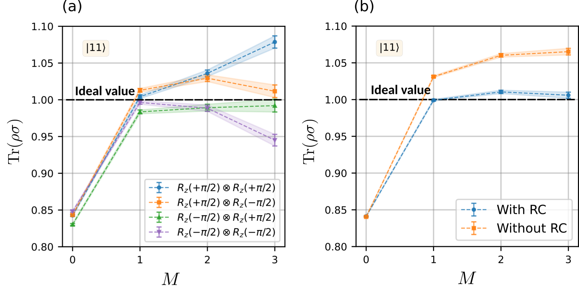
Supplementary Figure 9: Effect of coherent errors on the error-mitigated survival probability for a ten-swap experiment. The initial state is $|11\rangle$ and the ideal survival probability is 1 (dashed black lines). The thin colored areas connect small experimental error bars. All the plots show adaptive mitigation using $g(\mu)=\mu^{2}$. (a) Error-mitigated survival probability for different initial rotations. By comparing these results with the blue curve in Supplementary Figure 9(b), it becomes clear that averaging over the initial rotations substantially mitigates the preparation coherent error and enhances the QEM. (b) Error-mitigated survival probabilities obtained with RC (blue curve) and without RC (orange curve). The QEM accuracy is significantly increased by applying RC.

experiment, we present now a simulation of the same calibration process. The ideal CNOT gate is simulated through the unitary evolution

$$U=R_{Z}^{(0)}(-\pi/2)e^{-i\frac{\theta}{2}H_{\textrm{CR}}}R_{X}^{(1)}(-\pi/2),$$ (130)

with the cross-resonance interaction $H_{\textrm{CR}}=Z\otimes X$, and the rotations $R_{Z}^{(0)}(-\pi/2)=e^{i\frac{\pi}{4}Z}$ and $R_{X}^{(1)}(-\pi/2)=e^{i\frac{\pi}{4}X}$ acting on the target qubit and the control qubit, respectively. The angle $\theta$ depends on the strength and the duration of the pulse used to generate the cross-resonance interaction. An ideal (noise-free) CNOT gate corresponds to the angle $\theta=\pi/2$.

For the effect of noise, we consider the dissipator

$$\mathcal{L} =\xi\sum_{i=1}^{2}\gamma_{i}\left[A_{i}\otimes A_{i}^{\ast}-\frac{1}{2}A_{i}^{\dagger}A_{i}\otimes I-\frac{1}{2}I\otimes\left(A_{i}^{\dagger}A_{i}\right)^{\textrm{T}}\right],$$ (131)

$$A_{1} =Z,$$ (132)

$$A_{2} =\left(\begin{array}[]{cc}0&1\\ 0&0\end{array}\right),$$ (135)

where $\gamma_{1}=1$ and $\gamma_{2}=1/10$. In Supplementary Figures 10 and 11 we show the calibration curves for $\xi=2/100$ (Supplementary Figure 10) and $\xi=1/100$ (Supplementary Figure 11). Since the action of noise produces an imperfect CNOT gate, the angle $\theta$ obtained under a noisy calibration is in general different from $\pi/2$. We express this angle as $\theta=A_{\theta}\frac{\pi}{2}$, and take the “angle amplitude” $A_{\theta}$ as the parameter for calibration.

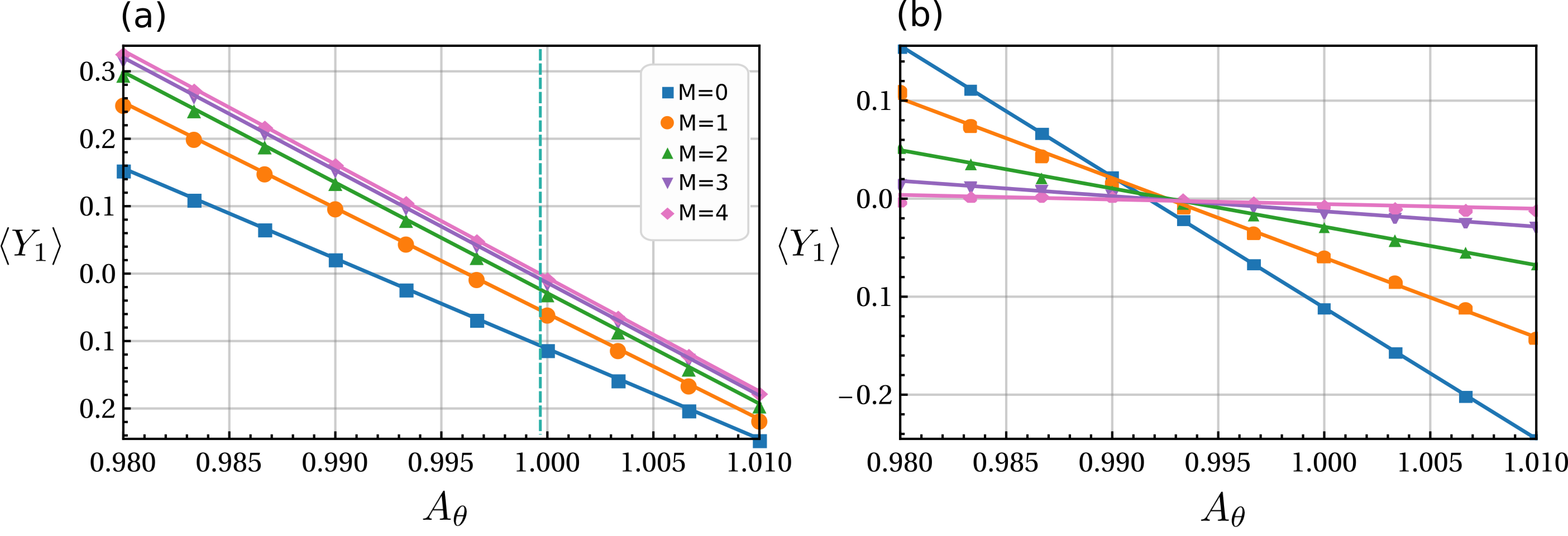
Supplementary Figure 10: Simulation of the calibration of a noisy CNOT gate, for noise strength $\xi=2/100$. The curves show the expectation value of $Y_{1}=I\otimes Y$ as a function of the angle amplitude $A_{\theta}$, which determines the angle $\theta=A_{\theta}\frac{\pi}{2}$ in the cross-resonance interaction $H_{CR}$ (cf. Eq. (130)). The calibrated amplitude corresponds to $\left\langle Y_{1}\right\rangle=0$ (cyan dashed line). Different curves stand for different mitigation orders $0\leq M\leq 4$. Figures (a) and (b) correspond to the application of the pulse inverse and the circuit inverse $\mathcal{K}_{\textrm{I}}=\mathcal{K}$, respectively.

As in the experimental case, the initial state and observable used for calibration are $\frac{1}{\sqrt{2}}\left(|0\rangle+|1\rangle\right)\otimes|0\rangle$ and $Y_{1}=I\otimes Y$, respectively. Furthermore, the target circuit consists of a sequence of 11 CNOTs, in order to increase the sensitivity of $\left\langle Y_{1}\right\rangle$ to variations of $A_{\theta}$. Therefore, the noisy target circuit and its inverse are given by

$$\mathcal{K} =\left(e^{-i\frac{\pi}{2}A_{\theta}\mathcal{H}_{\textrm{CR}}+\mathcal{L}}\right)^{11},$$ (136)

$$\mathcal{K}_{\textrm{I}} =\left(e^{i\frac{\pi}{2}A_{\theta}\mathcal{H}_{\textrm{CR}}+\mathcal{L}}\right)^{11},$$ (137)

where $\mathcal{H}_{\textrm{CR}}$ is the Liouville space representation of $H_{\textrm{CR}}$.

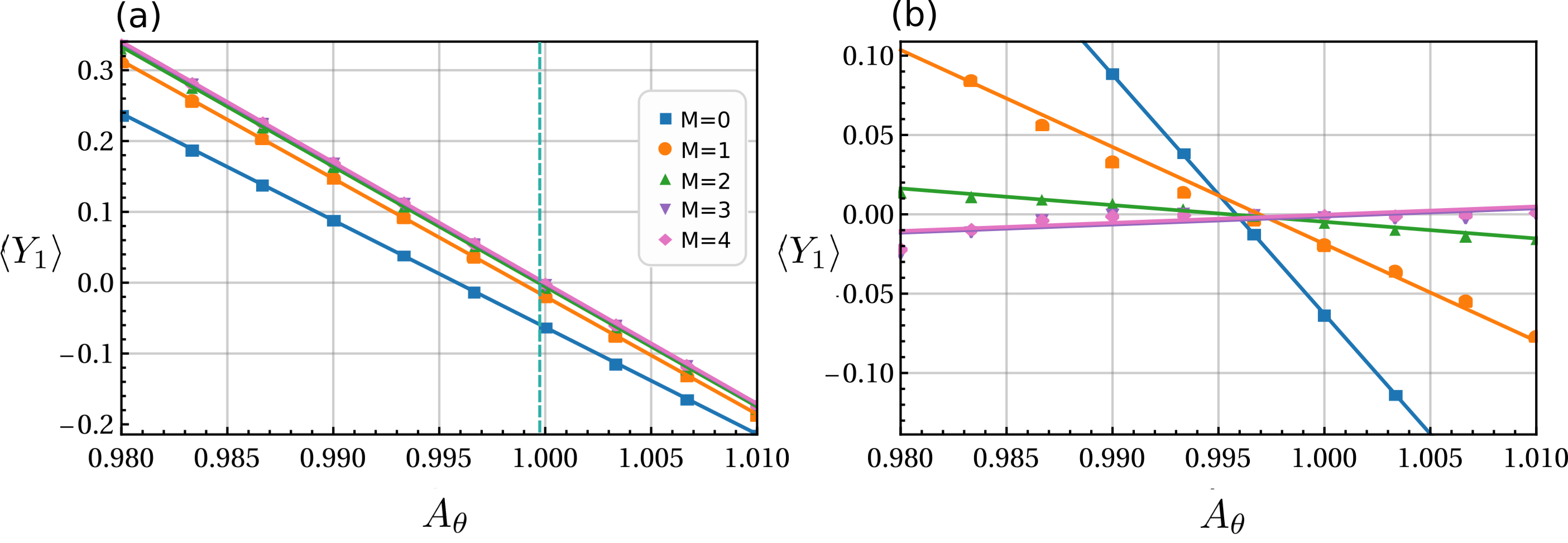
Supplementary Figure 11: Simulation of the calibration of a noisy CNOT gate, for noise strength $\xi=1/100$. The curves show the expectation value of $Y_{1}=I\otimes Y$ as a function of the angle amplitude $A_{\theta}$, which determines the angle $\theta=A_{\theta}\frac{\pi}{2}$ in the cross resonance interaction $H_{\textrm{CR}}$ (cf. Eq. (130)). The calibrated amplitude corresponds to $\left\langle Y_{1}\right\rangle=0$ (cyan dashed line). Different curves stand for different mitigation orders $0\leq M\leq 4$. Figures (a) and (b) correspond to the application of the pulse inverse and the circuit inverse $\mathcal{K}_{\textrm{I}}=\mathcal{K}$, respectively.

The amplitudes $A_{\theta}$ obtained for error mitigation orders $0\leq M\leq 4$ are given in Supplementary Table 3. Due to the small values of the noise strength $\xi$, we apply Taylor mitigation with the coefficients $a_{\textrm{Tay},m}^{(M)}$. In Supplementary Table 3, we can observe that $A_{\theta}$ tends to one as $M$ increases. This reflects the fact that higher mitigation orders produce an evolution $\mathcal{U}_{\textrm{KIK}}^{(M)}$ closer to the ideal CNOT gate, and therefore the resulting calibrated angle $\theta$ also approaches its noise-free value $\theta=\pi/2$. On the other hand, for the noisy calibration corresponding to $M=0$, the associated angle presents the largest deviation from $\theta=\pi/2$. As a consequence, such a biased angle gives rise to a coherent error.

$M$ (mitigation order)	0	1	2	3	4
$A_{\theta}$ for $\xi=2/100$	0.991671	0.996210	0.998235	0.999181	0.999631
$A_{\theta}$ for $\xi=1/100$	0.995830	0.998836	0.999673	0.999909	0.999977

Supplementary Table 3: Angle amplitudes $A_{\theta}$ obtained with KIK-based calibration of a CNOT gate. $A_{\theta}$ determines the angle $\theta=A_{\theta}\frac{\pi}{2}$ in Eq. (130), and $A_{\theta}=1$ for a noise-free CNOT. $\xi$ gives the noise strength in the dissipator (131).

To test the calibrated gate, we simulate the average gate fidelity after applying $M$th order Taylor mitigation to the noisy evolution

$$\mathcal{K}_{\textrm{CNOT}}=e^{-i\frac{\theta_{M}}{2}\mathcal{H}_{\textrm{CR}}+\mathcal{L}},$$ (138)

where $\theta_{M}$ is the angle calibrated via $M$th order mitigation. In other words, this strategy consists of using the same order of mitigation for the calibration of the CNOT and for the evaluation of its average fidelity.

The average gate fidelity between a quantum channel $\Lambda$ and a unitary evolution $U$ is defined by

$$F(\Lambda,U)=\int d\psi\langle\psi|U^{\dagger}\Lambda(|\psi\rangle\langle\psi|)U|\psi\rangle,$$ (139)

where the integral is taken over all the pure states $|\psi\rangle$ with respect to the Haar measure. Here, $\Lambda(|\psi\rangle\langle\psi|)$ denotes the state obtained by applying $\Lambda$ on $|\psi\rangle\langle\psi|$. For quantum channels acting on $N$ qubits, the fidelity (139) can be computed by using the Pauli transfer matrices of $\Lambda$ and $U$. The Pauli transfer matrix $R_{\Lambda}$ for a general quantum channel $\Lambda$ has elements ⁵³

$$\left(R_{\Lambda}\right)_{ij}=\frac{1}{d}\textrm{Tr}\left[P_{i}\Lambda\left(P_{j}\right)\right],$$ (140)

where $P_{i},P_{j}\in\{I,X,Y,Z\}^{\otimes N}$ are Pauli operators and $d=2^{N}$ is the dimension of the Hilbert space.

In this way, the fidelities $F_{M}$ in Supplementary Tables 4 and 5 are calculated as ⁵³

$$F(\Lambda,U)=\frac{\textrm{Tr}\left(R_{\Lambda}^{-1}R_{U}\right)+d}{d(d+1)},$$ (141)

with $U=e^{-i\frac{\theta}{2}H_{\textrm{CR}}}$ and the channel $\Lambda$ corresponding to $M$th order mitigation,

$$\mathcal{U}_{\textrm{KIK}}^{(M)} =\sum_{m=0}^{M}a_{\textrm{Tay},m}^{(M)}\mathcal{K}_{\textrm{CNOT}}\left(\mathcal{K}_{\textrm{I},\textrm{CNOT}}\mathcal{K}_{\textrm{CNOT}}\right)^{m},$$ (142)

$$\mathcal{K}_{\textrm{I},\textrm{CNOT}} =e^{i\frac{\theta_{M}}{2}\mathcal{H}_{\textrm{CR}}+\mathcal{L}}.$$ (143)

Using the Liouville space formalism, the matrix elements of $R_{\Lambda}$ and $R_{U}$ are given by

$$\left(R_{\Lambda}\right)_{ij} =\frac{1}{d}\langle P_{i}|\mathcal{U}_{\textrm{KIK}}^{(M)}|P_{j}\rangle,$$ (144)

$$\left(R_{U}\right)_{ij} =\frac{1}{d}\langle P_{i}|\mathcal{U}|P_{j}\rangle,$$ (145)

where $\mathcal{U}=U\otimes U^{\ast}$ and $|P_{j}\rangle$ is the vector representation of $P_{j}$. On the other hand, $F_{0}$ is computed by replacing $\mathcal{K}_{\textrm{CNOT}}$ and $\mathcal{K}_{\textrm{I},\textrm{CNOT}}$ in Eq. (142), by $e^{-i\frac{\theta_{0}}{2}\mathcal{H}_{\textrm{CR}}+\mathcal{L}}$ and $e^{i\frac{\theta_{0}}{2}\mathcal{H}_{\textrm{CR}}+\mathcal{L}}$, respectively.

We choose Taylor mitigation because the corresponding coefficients do not depend on the initial state. In contrast, in the case of adaptive mitigation the quantity $\mu=\langle\rho|\mathcal{K}_{\textrm{I},\textrm{CNOT}}\mathcal{K}_{\textrm{CNOT}}|\rho\rangle$ depends on the initial state $\rho$, which makes it difficult to take into account when evaluating the gate fidelity.

$M$ (mitigation order)	$F_{0}$ (noisy calibration)	$F_{M}$ (KIK-based calibration)	$F_{0}$ with RC
0	0.967325	0.967325	0.967325
1	0.997270	0.997298	0.997388
2	0.999692	0.999725	0.999743
3	0.999934	0.999968	0.999972
4	0.999961	0.999996	0.999997

Supplementary Table 4: KIK-mitigated gate fidelity (141) (simulation) for a CNOT gate affected by noise (131), with noise strength $\xi=2/100$. $F_{0}$ is the fidelity obtained when the gate is calibrated without KIK error mitigation. $F_{M}$ is the fidelity when $M$th order mitigation is performed alongside $M$th order KIK calibration. “$F_{0}$ with RC” refers to the fidelity obtained without KIK-based calibration, and by combining KIK mitigation with RC. In this case the fidelity is the average over fidelities associated with all the 16 RC operations described in Supplementary Table 1.

Supplementary Tables 4 and 5 show the simulated fidelities for $\xi=2/100$ and $\xi=1/100$, respectively. The second column in these tables gives the error-mitigated fidelities without a KIK-based calibration, i.e. when $\theta_{M}=\theta_{0}$. The third column contains the values simulated by following the $M$-order mitigation strategy previously described. Finally, fidelities obtained without KIK-based calibration and RC integrated into the KIK mitigation are presented in the fourth column. Both tables show that KIK-based calibration and RC yield similar fidelities, which surpass the values obtained when none of these methods is employed. The effect of these two approaches is different though. On the one hand, RC mitigates the coherent error that characterizes the biased angle $\theta_{0}$ by postprocessing measurement data. On the other hand, in the KIK-based calibration this coherent error is reduced at a physical level.

$M$ (mitigation order)	$F_{0}$ (noisy calibration)	$F_{M}$ (KIK-based calibration)	$F_{0}$ with RC
0	0.983434	0.983434	0.983434
1	0.999288	0.999296	0.999320
2	0.999954	0.999963	0.999965
3	0.999989	0.999998	0.999998
4	0.999991	1.000000	1.000000

Supplementary Table 5: KIK-mitigated gate fidelity (141) (simulation) for a CNOT gate affected by noise (131), with noise strength $\xi=1/100$. The description of each column is as in Supplementary Table 4.

Supplementary Note 7: Numerical example to illustrate saturation of the KIK formula

In this section, we consider a numerical example where the accuracy of QEM using the KIK method saturates at approximately the mitigation order $M=4$. We quantify the accuracy by the relative error

$$\frac{\varepsilon_{\textrm{KIK}}^{(M)}}{|\langle A|\mathcal{U}|\rho\rangle|}=\frac{\left|\langle A|\mathcal{U}|\rho\rangle-\langle A|\mathcal{U}_{\textrm{KIK}}^{(M)}|\rho\rangle\right|}{|\langle A|\mathcal{U}|\rho\rangle|},$$ (146)

where $\varepsilon_{\textrm{KIK}}^{(M)}=\left|\langle A|\mathcal{U}|\rho\rangle-\langle A|\mathcal{U}_{\textrm{KIK}}^{(M)}|\rho\rangle\right|$ is the difference between the ideal expectation value $\langle A|\mathcal{U}|\rho\rangle$, and the error-mitigated expectation value $\langle A|\mathcal{U}_{\textrm{KIK}}^{(M)}|\rho\rangle$, for the observable $A$ and the initial state $\rho$. In our example, the error (146) first decreases as a function of $M$, and then attains a value approximately constant for $M\geq 4$. This is shown in Supplementary Figure 12. We apply QEM with Taylor mitigation, characterized by $\mathcal{U}_{\textrm{KIK}}^{(M)}=\sum_{m=0}^{M}a_{\textrm{Tay},m}^{(M)}\mathcal{K}\left(\mathcal{K}_{\textrm{I}}\mathcal{K}\right)^{m}$, and the coefficients $a_{\textrm{Tay},m}^{(M)}$ in Eq. (77).

Our example refers to a four-qubit system characterized by the time-independent Hamiltonian

$$H =X\otimes X\otimes I\otimes I+I\otimes X\otimes X\otimes I+I\otimes I\otimes X\otimes X,$$ (147)

$$\mathcal{H} =H\otimes I-I\otimes H^{\textrm{T}},$$ (148)

where $X=\left(\begin{array}[]{cc}0&1\\ 1&0\end{array}\right)$ and $I=\left(\begin{array}[]{cc}1&0\\ 0&1\end{array}\right)$. Here, $\mathcal{H}$ is the Liouville space representation of $H$, taking into account Eq. (5). Each qubit is subjected to spontaneous emission, which can be described via a GKLS (Gorini-Kossakowski-Sudarshan-Lindblad) master equation with dissipator $\hat{L}$ such that

$$\hat{L}[\rho] =\sum_{k=1}^{4}\xi_{k}\left(A_{k}\rho A_{k}^{\dagger}-\frac{1}{2}A_{k}^{\dagger}A_{k}\rho-\frac{1}{2}\rho A_{k}^{\dagger}A_{k}\right),$$ (149)

$$A_{1} =\left(\begin{array}[]{cc}0&1\\ 0&0\end{array}\right)\otimes I\otimes I\otimes I,$$ (152)

$$A_{2} =I\otimes\left(\begin{array}[]{cc}0&1\\ 0&0\end{array}\right)\otimes I\otimes I,$$ (155)

$$A_{3} =I\otimes I\otimes\left(\begin{array}[]{cc}0&1\\ 0&0\end{array}\right)\otimes I,$$ (158)

$$A_{4} =I\otimes I\otimes I\otimes\left(\begin{array}[]{cc}0&1\\ 0&0\end{array}\right).$$ (161)

We assume that all the qubits are affected by the same relaxation rate $\xi=\xi_{k}=0.02$, for $1\leq k\leq 4$. Using the vectorization rule (cf. Eq. (5)), in Liouville space the dissipator (149) takes the form

$$\mathcal{L}=\xi\sum_{k=1}^{4}\left(A_{k}\otimes A_{k}^{\ast}-\frac{1}{2}A_{k}^{\dagger}A_{k}\otimes I-\frac{1}{2}I\otimes A_{k}^{\dagger}A_{k}\right),$$ (162)

where $A_{k}^{\ast}$ denotes the complex conjugate of $A_{k}$.

Assuming a time unit $T=1$ for the evolution time, we have that

$$\mathcal{U} =e^{-i\mathcal{H}},$$ (163)

$$\mathcal{K} =e^{-i\mathcal{H}+\mathcal{L}},$$ (164)

$$\mathcal{K}_{\textrm{I}} =e^{i\mathcal{H}+\mathcal{L}}.$$ (165)

The total system starts in the ground state $\rho=\left(\begin{array}[]{cc}1&0\\ 0&0\end{array}\right)^{\otimes 4}$, whose vector form is given by $|\rho\rangle=(1,0,0,...,0)^{\textrm{T}}$. The observable $A$ is the projector onto the ground state, and thus $\langle A|=(1,0,0,...,0)$.

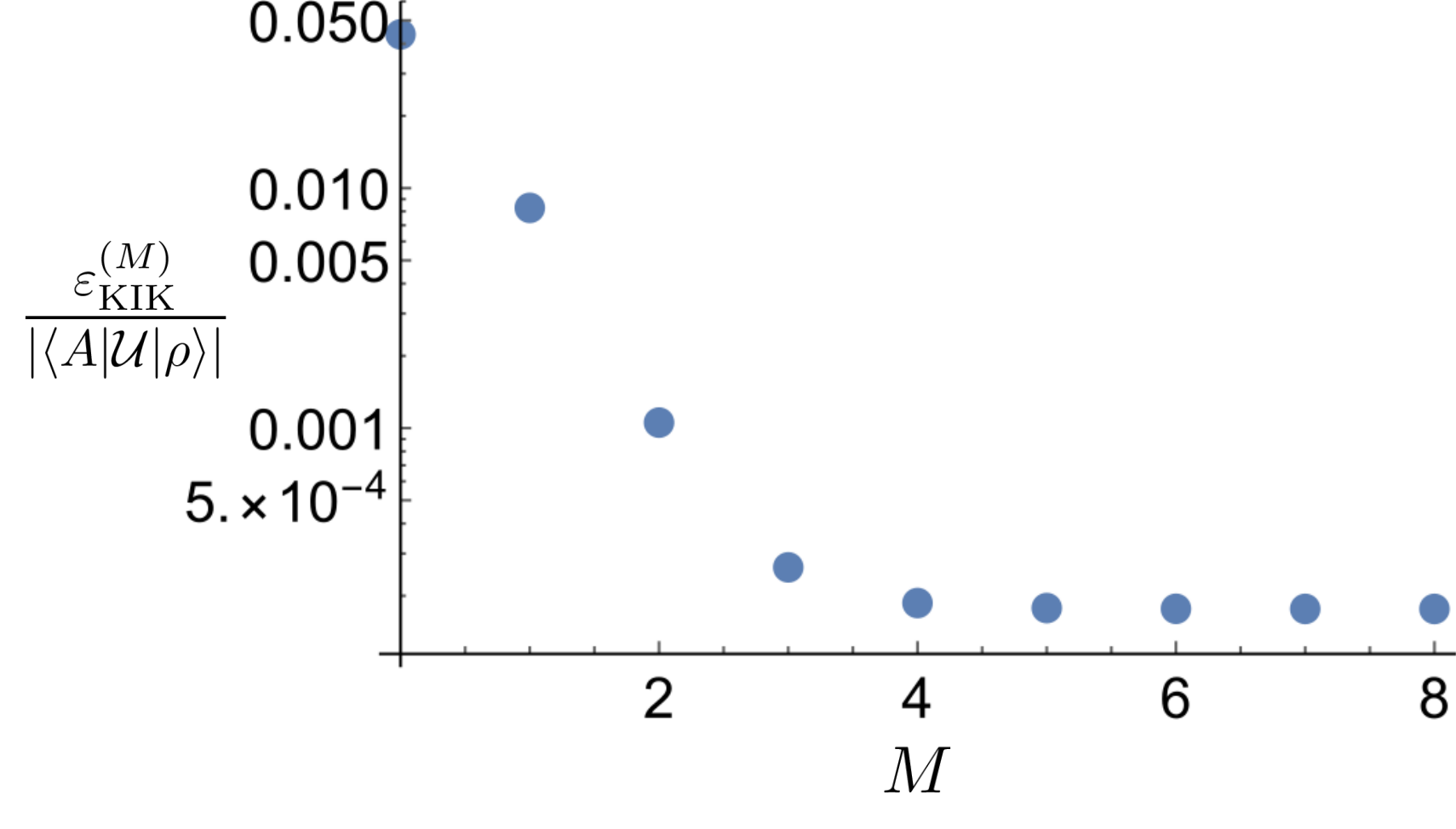
Supplementary Figure 12: Log scale plot of the relative error (146), for the QEM example described in the present supplementary note.

The saturation of the relative error can be understood as being a consequence of the approximations involved in the derivation of the KIK formula. More specifically, it is related to the fact that in the derivation of Eq. (26) we have discarded higher-order Magnus terms $\Omega_{n\geq 2}$. Nevertheless, it is worth noting that, according to Supplementary Figure 12, a relative error as small as $\sim 10^{-4}$ can already be achieved with a mitigation order $M=3$. When the initial error is smaller (i.e. when $\xi$ is smaller), the improvement is even more substantial.

Supplementary Note 8: Derivation of upper bounds for the performance of the KIK method

A complete assessment of a QEM technique requires establishing bounds for the remaining error in the estimation of expectation values. Furthermore, these bounds should be applicable to general observables $A$ and circuits $\mathcal{K}$ of arbitrary size. The goal of the present section is to derive such bounds, in the case of QEM using the KIK method. In the fisrt two subsections we will state some technical results and physically realistic assumptions, which will be used for the derivation of our bounds in the last two subsections.

Lower bound on the smallest eigenvalue of $\mathcal{K}_{\textrm{I}}\mathcal{K}$. Assuming that $\mathcal{K}_{\textrm{I}}\mathcal{K}$ is diagonalizable, i.e. $\mathcal{K}_{\textrm{I}}\mathcal{K}=\sum_{k}\lambda_{k}|k)(k|$, where $|k)$ and $(k|$ denote respectively right and left eigenvectors (note that in general we may have $(k|\neq|k)^{\dagger}$), we will obtain the bound

$$\textrm{min}_{k}\lambda_{k}\geq e^{-2\intop_{0}^{T}\left\|\mathcal{L}(t)\right\|dt}.$$ (166)

We recall that $\mathcal{L}(t)$ is the dissipator introduced in Eq. (10), and $T$ is the evolution time for $\mathcal{K}$. The norm $\left\|\ast\right\|$ in Eq (166) is the spectral norm.

First, we consider the equivalent expression of Eq. (20),

$$\frac{d}{dt}\tilde{\mathcal{K}}_{\textrm{int}}(t)=\tilde{\mathcal{L}}_{\textrm{int}}(t)\tilde{\mathcal{K}}_{\textrm{int}}(t),$$ (167)

with the interaction-picture evolution $\tilde{\mathcal{K}}_{\textrm{int}}(t)=\tilde{\mathcal{U}}^{\dagger}(t)\tilde{\mathcal{K}}(t)$, and dissipator $\tilde{\mathcal{L}}_{\textrm{int}}(t)=\tilde{\mathcal{U}}^{\dagger}(t)\tilde{\mathcal{L}}(t)\tilde{\mathcal{U}}(t)$. We point out that, in this case, we consider only the time interval $0\leq t\leq T$. The inverse evolution $\tilde{\mathcal{K}}_{\textrm{int}}^{-1}(t)=\tilde{\mathcal{K}}^{-1}(t)\tilde{\mathcal{U}}(t)$ satisfies the equation

$$\frac{d}{dt}\tilde{\mathcal{K}}_{\textrm{int}}^{-1}(t)=-\tilde{\mathcal{L}}_{\textrm{int}}(T-t)\tilde{\mathcal{K}}_{\textrm{int}}^{-1}(t),$$ (168)

which will be used in the derivation of (166). Here, it is important to remark that $\tilde{\mathcal{K}}_{\textrm{int}}^{-1}(t)$ is the mathematical inverse of $\tilde{\mathcal{K}}_{\textrm{int}}(t)$ and must not be confused with $\mathcal{K}_{\textrm{I}}$.

By taking the spectral norm at both sides of Eq. (168), we get

$$\left\|\frac{d}{dt}\tilde{\mathcal{K}}_{\textrm{int}}^{-1}(t)\right\| =\left\|\tilde{\mathcal{L}}_{\textrm{int}}(T-t)\tilde{\mathcal{K}}_{\textrm{int}}^{-1}(t)\right\|$$

$$\leq\left\|\tilde{\mathcal{L}}(T-t)\right\|\left\|\tilde{\mathcal{K}}^{-1}(t)\right\|,$$ (169)

where the inequality follows from the submultiplicativity and unitary invariance of the spectral norm. On the other hand, we can apply the reverse triangle inequality $\left\|x-y\right\|\geq\left|\left\|x\right\|-\left\|y\right\|\right|$ to obtain

$$\left\|\frac{d}{dt}\tilde{\mathcal{K}}_{\textrm{int}}^{-1}(t)\right\| =\textrm{lim}_{\Delta t\rightarrow 0}\left\|\frac{\tilde{\mathcal{K}}_{\textrm{int}}^{-1}(t+\Delta t)-\tilde{\mathcal{K}}_{\textrm{int}}^{-1}(t)}{\Delta t}\right\|$$

$$\geq\textrm{lim}_{\Delta t\rightarrow 0}\left|\frac{\left\|\tilde{\mathcal{K}}_{\textrm{int}}^{-1}(t+\Delta t)\right\|-\left\|\tilde{\mathcal{K}}_{\textrm{int}}^{-1}(t)\right\|}{\Delta t}\right|$$

$$=\frac{d}{dt}\left\|\tilde{\mathcal{K}}_{\textrm{int}}^{-1}(t)\right\|=\frac{d}{dt}\left\|\tilde{\mathcal{K}}^{-1}(t)\right\|.$$ (170)

By combining this result with Eq. (169), we have the inequality

$$\frac{d}{dt}\left\|\tilde{\mathcal{K}}^{-1}(t)\right\|\leq\left\|\tilde{\mathcal{L}}(T-t)\right\|\left\|\tilde{\mathcal{K}}^{-1}(t)\right\|,$$ (171)

which upon integration yields

$$\left\|\tilde{\mathcal{K}}^{-1}(T)\right\|\leq e^{\intop_{0}^{T}\left\|\mathcal{\tilde{\mathcal{L}}}(T-t)\right\|dt}.$$ (172)

Taking into account that $\tilde{\mathcal{K}}(T)=\mathcal{K}$ and $\mathcal{\tilde{\mathcal{L}}}(T-t)=\mathcal{L}(T-t)$ for $0\leq t\leq T$ (cf. Eq. (17)), the change of variable $t^{\prime}=T-t$ straightforwardly leads to

$$\left\|\mathcal{K}^{-1}\right\|\leq e^{\intop_{0}^{T}\left\|\mathcal{L}(t)\right\|dt}.$$ (173)

Consider now the singular value decomposition (SVD) $\mathcal{K}=\mathcal{V}\mathcal{S}\mathcal{W}$, where $\mathcal{S}$ is a diagonal matrix with the singular values of $\mathcal{K}$ and $\mathcal{V}$ and $\mathcal{W}$ are unitary matrices. Then, the SVD of $\mathcal{K}^{-1}$ reads $\mathcal{W}^{\dagger}\mathcal{S}^{-1}\mathcal{V}^{\dagger}$, and the spectral norm (maximum singular value) of $\mathcal{K}^{-1}$ is given by $\left\|\mathcal{K}^{-1}\right\|=1/s_{\textrm{min}}$, where $s_{\textrm{min}}$ is the minimum singular value of $\mathcal{K}$. Accordingly, we can rewrite (173) as

$$s_{\textrm{min}}\geq e^{-\intop_{0}^{T}\left\|\mathcal{L}(t)\right\|dt}.$$ (174)

The singular values of $\mathcal{K}$ are the eigenvalues of $\left(\mathcal{K}^{\dagger}\mathcal{K}\right)^{\frac{1}{2}}$, where $\mathcal{K}^{\dagger}$ is the Hermitian conjugate of $\mathcal{K}$. If the evolution $\mathcal{K}_{\textrm{I}}$ coincides with $\mathcal{K}^{\dagger}$, we have that $s_{\textrm{min}}$ is also the minimum eigenvalue of $\left(\mathcal{K}_{\textrm{I}}\mathcal{K}\right)^{\frac{1}{2}}$, or, equivalently, the minimum eigenvalue of $\mathcal{K}_{\textrm{I}}\mathcal{K}$ satisfies the inequality (166). Hence, our last step in proving this inequality is to show that $\mathcal{K}_{\textrm{I}}=\mathcal{K}^{\dagger}$, under sound physical conditions. This is done in the next subsection.

Sufficient condition for $\mathcal{K}_{\textrm{I}}=\mathcal{K}^{\dagger}$. Suppose that the dissipator $\mathcal{L}(t)$ is Hermitian, i.e. $\mathcal{L}^{\dagger}(t)=\mathcal{L}(t)$ for $0\leq t\leq T$. Then, from the definition of the first-order Magnus term (22) it also follows that

$$\Omega_{1}^{\dagger}(T)=\Omega_{1}(T).$$ (175)

If we can prove that, up to first order in the Magnus expansion (where $\Omega(T)$ is approximated by $\Omega_{1}(T)$),

$$\mathcal{K}_{\textrm{I}}\approx e^{\Omega_{1}(T)}\mathcal{U}^{\dagger},$$ (176)

then, Eqs. (23) and (176) imply that $\mathcal{K}_{\textrm{I}}=\mathcal{K}^{\dagger}$ within this approximation.

Before discussing under which circumstances the property $\mathcal{L}^{\dagger}(t)=\mathcal{L}(t)$ is satisfied, let us first derive Eq. (176). We start by writing the formal solution to the inverse evolution $\mathcal{K}_{\textrm{I}}$. Denoting the corresponding Magnus expansion by $\Omega_{I}$, and assuming for simplicity that $\mathcal{L}_{\textrm{I}}(t)$ acts on the time interval $(0,T)$ (as opposed to the interval $(T,2T)$, used in the derivation of the KIK formula), Eq. (23) leads to

$$\mathcal{K}_{\textrm{I}} =\mathcal{U}^{\dagger}e^{\Omega_{\textrm{I}}(T)}$$

$$\approx\mathcal{U}^{\dagger}e^{\Omega_{\textrm{I},1}(T)},$$ (177)

with the first-order Magnus term

$$\Omega_{\textrm{I},1}(T) =\int_{0}^{T}\mathcal{L}_{\textrm{I},\textrm{int}}(t)dt$$

$$=\int_{0}^{T}\mathcal{U}(t)\mathcal{L}(T-t)\mathcal{U}^{\dagger}(t)dt.$$ (178)

Writing $\mathcal{U}(t)$ as $\mathcal{U}(t)=\mathcal{U}(T)\mathcal{U}^{\dagger}(T-t)$, and performing the change of variable $t^{\prime}=T-t$ in the integral, we obtain

$$\Omega_{\textrm{I},1}(T) =-\mathcal{U}(T)\left(\int_{T}^{0}\mathcal{U}^{\dagger}(t^{\prime})\mathcal{L}(t^{\prime})\mathcal{U}(t^{\prime})dt^{\prime}\right)\mathcal{U}^{\dagger}(T)$$

$$=\mathcal{U}\left(\int_{0}^{T}\mathcal{U}^{\dagger}(t^{\prime})\mathcal{L}(t^{\prime})\mathcal{U}(t^{\prime})dt^{\prime}\right)\mathcal{U}^{\dagger}$$

$$=\mathcal{U}\Omega_{1}(T)\mathcal{U}^{\dagger}.$$ (179)

Note that we also used the simplified notation $\mathcal{U}(T)=\mathcal{U}$. In this way, we conclude that

$$\mathcal{K}_{\textrm{I}} \approx\mathcal{U}^{\dagger}e^{\mathcal{U}\Omega_{1}(T)\mathcal{U}^{\dagger}}$$

$$=e^{\Omega_{1}(T)}\mathcal{U}^{\dagger}.$$ (180)

Thus, the hermiticity of $\mathcal{L}(t)$ leads to $\mathcal{K}_{\textrm{I}}=\mathcal{K}^{\dagger}$, within our approximation.

Now, let us come back to the subject of the Hermiticity of $\mathcal{L}(t)$. A sufficient condition to have this property is that

$$\mathcal{L}(t)=\sum_{\vec{\mathbf{k}}}\alpha_{\vec{\mathbf{k}}}(t)\left(P_{\vec{\mathbf{k}}}\otimes P_{\vec{\mathbf{k}}}^{\textrm{T}}-\mathcal{I}\right),$$ (181)

where $P_{\vec{\mathbf{k}}}=\sigma_{\mathbf{k}_{1}}^{(1)}\otimes\sigma_{\mathbf{k}_{2}}^{(2)}\otimes...\otimes\sigma_{\mathbf{k}_{n}}^{(n)}\otimes...\otimes\sigma_{\mathbf{k}_{N}}^{(N)}$ is a Pauli operator acting on $N$ qubits, $\sigma_{\mathbf{k}_{n}}^{(n)}\in\left\{I,X,Y,Z\right\}$ is a Pauli matrix acting on the $n$th qubit, and the time-dependent coefficients $\alpha_{\vec{\mathbf{k}}}(t)$ are real. We note that a time-independent version of this dissipator was recently considered in Ref. ²⁰. For a given state $\rho$, we can check by direct application of the identity (5) that Eq. (181) is the Liouville space representation of the superoperator $\hat{L}(t)$ such that

$$\hat{L}(t)[\rho]=\sum_{\vec{\mathbf{k}}}\alpha_{\vec{\mathbf{k}}}(t)(P_{\vec{\mathbf{k}}}\rho P_{\vec{\mathbf{k}}}-\rho).$$ (182)

The noise model of Ref. ²⁰ relies on a time-independent $\hat{L}(t)=\hat{L}$, characterized by time-independent coefficients $\alpha_{\vec{\mathbf{k}}}(t)=\alpha_{\vec{\mathbf{k}}}$. In addition, $\alpha_{\vec{\mathbf{k}}}\neq 0$ only if the index $\vec{\mathbf{k}}=\{\mathbf{k}_{1},\mathbf{k}_{2},...,\mathbf{k}_{N}\}$ contains at most two components $\mathbf{k}_{n}$ different from 0, which limits correlated errors to occur at most between pairs of qubits. On the other hand, the more general dissipator (181) guarantees the condition $\mathcal{K}_{\textrm{I}}=\mathcal{K}^{\dagger}$. We remark that the time-dependent coefficients $\alpha_{\vec{\mathbf{k}}}(t)$ in Eq. (181) can also be different from zero for arbitrary indices $\vec{\mathbf{k}}$, thereby allowing for correlated errors between any number of qubits in the system.

The Pauli channel (181) arises naturally when executing RC for the purpose of mitigating coherent errors. In others words, by applying RC on a general dissipator, which can contain non-diagonal components in the Pauli operator representation, a dissipator of the form (181) is obtained. Since we exploit RC in our experiments, the effective noise is described by a Pauli channel, which according to the above results implies $\mathcal{K}_{\textrm{I}}=\mathcal{K}^{\dagger}$.

First error bounds for Adaptive mitigation and Taylor mitigation. To begin this subsection, we recall that the error-mitigated evolution $\mathcal{U}_{\textrm{KIK}}=\mathcal{K}\left(\mathcal{K}_{\textrm{I}}\mathcal{K}\right)^{-\frac{1}{2}}$ is implemented through $M$-order approximations of the form $\mathcal{U}_{\textrm{KIK}}^{(M)}=\sum_{m=0}^{M}a_{m}^{(M)}\mathcal{K}\left(\mathcal{K}_{\textrm{I}}\mathcal{K}\right)^{m}$. Our goal is to obtain an upper bound on the error

$$\varepsilon_{\textrm{KIK}}^{(M)}=\left|\langle A|\mathcal{U}|\rho\rangle-\langle A|\mathcal{U}_{\textrm{KIK}}^{(M)}|\rho\rangle\right|,$$ (183)

which quantifies how much the ideal expectation value $\langle A|\mathcal{U}|\rho\rangle$ deviates from the error-mitigated expectation value $\langle A|\mathcal{U}_{\textrm{KIK}}^{(M)}|\rho\rangle$. Here, $A$ is an arbitrary observable and $\rho$ is an arbitrary initial state.

We will start by deriving a bound for the error associated with adaptive mitigation, with the coefficients ${\color[rgb]{1,0,0}{\normalcolor a_{\textrm{Adap},m}^{(M)}}}[g(\mu)]$ evaluated at $g(\mu)=\mu$, and $1\leq M\leq 3$. The possibility of obtaining tighter bounds with different choices of $g(\mu)$ is left as an open problem. Later on, we will derive another bound that, despite being looser, has the advantage of being independent of $\mu$, and is also valid for both adaptive mitigation with $g(\mu)=\mu$ and Taylor mitigation.

Using our conventional approximations $\mathcal{K}\approx\mathcal{U}e^{\Omega_{1}}$ and $\mathcal{K}_{\textrm{I}}\mathcal{K}\approx e^{2\Omega_{1}}$, we can write $\mathcal{U}_{\textrm{KIK}}^{(M)}$ as

$$\mathcal{U}_{\textrm{KIK}}^{(M)} \approx\mathcal{U}\sum_{m=0}^{M}{\color[rgb]{1,0,0}{\normalcolor a_{\textrm{Adap},m}^{(M)}}}(\mu)e^{(2m+1)\Omega_{1}}$$

$$\approx\mathcal{U}\sum_{m=0}^{M}{\color[rgb]{1,0,0}{\normalcolor a_{\textrm{Adap},m}^{(M)}}}(\mu)\left(\mathcal{K}_{\textrm{I}}\mathcal{K}\right)^{m+1/2}.$$ (184)

Therefore,

$$\varepsilon_{\textrm{KIK}}^{(M)} =\left|\langle A|\left(\mathcal{U}-\mathcal{U}_{\textrm{KIK}}^{(M)}\right)|\rho\rangle\right|$$

$$\leq\sqrt{\langle A|A\rangle}\sqrt{\langle\rho|\rho\rangle}\left\|\mathcal{U}\left(\mathcal{I}-\sum_{m=0}^{M}{\color[rgb]{1,0,0}{\normalcolor a_{\textrm{Adap},m}^{(M)}}}(\mu)\left(\mathcal{K}_{\textrm{I}}\mathcal{K}\right)^{m+1/2}\right)\right\|$$

$$=\sqrt{\langle A|A\rangle}\left\|\left(\mathcal{I}-\sum_{m=0}^{M}{\color[rgb]{1,0,0}{\normalcolor a_{\textrm{Adap},m}^{(M)}}}(\mu)\left(\mathcal{K}_{\textrm{I}}\mathcal{K}\right)^{m+1/2}\right)\right\|,$$ (185)

where the first inequality follows from the definition (184) and the definition of the spectral norm $\left\|*\right\|$. In the last line, we use the unitary invariance of this norm. Moreover, we assume an initial pure state $\rho$, which implies $\langle\rho|\rho\rangle=1$. Assuming as before that $\mathcal{L}(t)$ satisfies Eq. (181), and hence $\mathcal{K}_{\textrm{I}}=\mathcal{K}^{\dagger}$, we have that the operator $\mathcal{K}_{\textrm{I}}\mathcal{K}$ is Hermitian. Since this implies that $\mathcal{I}-\sum_{m=0}^{M}{\color[rgb]{1,0,0}{\normalcolor a_{\textrm{Adap},m}^{(M)}}}(\mu)\left(\mathcal{K}_{\textrm{I}}\mathcal{K}\right)^{m+1/2}$ is also Hermitian, the corresponding spectral norm is simply the absolute value of its maximum eigenvalue. In this way, Eq. (185) leads to

$$\varepsilon_{\textrm{KIK}}^{(M)}\leq\sqrt{\langle A|A\rangle}\textrm{max}_{k}\left|1-\sum_{m=0}^{M}{\color[rgb]{1,0,0}{\normalcolor a_{\textrm{Adap},m}^{(M)}}}(\mu)\left(\lambda_{k}\right)^{m+1/2}\right|,$$ (186)

where we have again denoted the eigenvalues of $\mathcal{K}_{\textrm{I}}\mathcal{K}=\sum_{k}\lambda_{k}|k\rangle\langle k|$ by $\{\lambda_{k}\}$. Since these eigenvalues may be difficult to evaluate both experimentally and theoretically, we establish another upper bound to $\varepsilon_{\textrm{KIK}}^{(M)}$ that depends on the single quantity $\intop_{0}^{T}\left\|\mathcal{L}(t)\right\|dt$, instead of all the eigenvalues $\lambda_{k}$.

We start by looking at the behavior of the function $f_{M}(\mu,\lambda):=\left|1-\sum_{m=0}^{M}{\color[rgb]{1,0,0}{\normalcolor a_{\textrm{Adap},m}^{(M)}}}(\mu)\left(\lambda\right)^{m+1/2}\right|$ in the plots of Supplementary Figure 13. This will allow us to derive the bound

$$\varepsilon_{\textrm{KIK}}^{(M)}\leq\sqrt{\langle A|A\rangle}\left|1-\sum_{m=0}^{M}{\color[rgb]{1,0,0}{\normalcolor a_{\textrm{Adap},m}^{(M)}}}(\mu)\left(e^{-2\intop_{0}^{T}\left\|\mathcal{L}(t)\right\|dt}\right)^{m+1/2}\right|,$$ (187)

for $M=1,2,3$. To this end, we note that the right hand side of Eq. (186) can be written as $\sqrt{\langle A|A\rangle}$$\textrm{max}_{k}f_{M}(\mu,\lambda_{k})$. Thus, we will obtain the bound (187) by proving the inequality $\textrm{max}_{k}f_{M}(\mu,\lambda_{k})\leq f_{M}\left(\mu,e^{-2\intop_{0}^{T}\left\|\mathcal{L}(t)\right\|dt}\right)$, for $M=1,2,3$. First, we will show that this inequality holds when the eigenvalue that maximizes $f_{M}(\mu,\lambda_{k})$ is smaller than $\mu$, and then the proof will be extended to the complementary case (i.e. when the aforementioned eigenvalue is larger than $\mu$).

For the first case we resort to the plots (a), (b) and (c) in Supplementary Figure 13. These plots show that if $\lambda\leq\mu$, the function $f_{M}(\mu,\lambda)$ is monotonically decreasing with respect to $\lambda$. Therefore, the inequality $\textrm{min}_{k}\lambda_{k}\geq e^{-2\intop_{0}^{T}\left\|\mathcal{L}(t)\right\|dt}$ (cf. Eq. (166)) implies that

$$f_{M}(\mu,\lambda_{k})\leq f_{M}(\mu,\textrm{min}_{k}\lambda_{k})\leq f_{M}\left(\mu,e^{-2\intop_{0}^{T}\left\|\mathcal{L}(t)\right\|dt}\right),$$ (188)

for any eigenvalue $\lambda_{k}$ such that $\lambda_{k}\leq\mu$.

If $\lambda\geq\mu$, the plots (d), (e) and (f) in Supplementary Figure 13 show that $f_{M}(\mu,\lambda)\leq f_{M}(\mu,\mu)$. Since

$$\mu=\langle\rho|\mathcal{K}_{\textrm{I}}\mathcal{K}|\rho\rangle=\sum_{k}\lambda_{k}|\langle k|\rho\rangle|^{2}\geq\textrm{min}_{k}\lambda_{k},$$ (189)

the monotonicity observed in Supplementary Figures 13(a)-13(c) leads to $f_{M}(\mu,\lambda)\leq f_{M}(\mu,\mu)\leq f_{M}(\mu,\textrm{min}_{k}\lambda_{k})$, where the rightmost inequality is a consequence of (189) and the leftmost inequality follows by hypothesis ($\lambda\geq\mu$). Therefore, the inequalities (188) also hold when $\lambda_{k}\geq\mu$. This implies that $\textrm{max}_{k}f_{M}(\mu,\lambda_{k})\leq f_{M}\left(\mu,e^{-2\intop_{0}^{T}\left\|\mathcal{L}(t)\right\|dt}\right)$, because (188) is valid for any eigenvalue $\lambda_{k}$.

Next, we derive another bound that is independent of both $\lambda_{k}$ and $\mu$. In this case, we will use the monotonicity of $f_{M}(\mu,\lambda)$ with respect to $\mu$, for $\mu\geq\lambda$ (see Supplementary Figures 13(a)-13(c)). By combining $\textrm{min}_{k}\lambda_{k}\geq e^{-2\intop_{0}^{T}\left\|\mathcal{L}(t)\right\|dt}$ (Eq. (166)) with Eq. (189), we have that $\mu,1\geq$$e^{-2\intop_{0}^{T}\left\|\mathcal{L}(t)\right\|dt}$ and therefore $f_{M}\left(\mu,e^{-2\intop_{0}^{T}\left\|\mathcal{L}(t)\right\|dt}\right)\leq f_{M}\left(1,e^{-2\intop_{0}^{T}\left\|\mathcal{L}(t)\right\|dt}\right)$. By combining this result with Eq. (187), we obtain the bound

$$\varepsilon_{\textrm{KIK}}^{(M)} \leq\sqrt{\langle A|A\rangle}f_{M}\left(\mu,e^{-2\intop_{0}^{T}\left\|\mathcal{L}(t)\right\|dt}\right)$$

$$\leq\sqrt{\langle A|A\rangle}f_{M}\left(1,e^{-2\intop_{0}^{T}\left\|\mathcal{L}(t)\right\|dt}\right)$$

$$=\sqrt{\langle A|A\rangle}\left|1-\sum_{m=0}^{M}{\color[rgb]{1,0,0}{\normalcolor a_{\textrm{Adap},m}^{(M)}}}(1)\left(e^{-2\intop_{0}^{T}\left\|\mathcal{L}(t)\right\|dt}\right)^{m+1/2}\right|,$$ (190)

for $M=1,2,3$. Although this bound is looser than (187), it only depends on $\intop_{0}^{T}\left\|\mathcal{L}(t)\right\|dt$. Since this quantity is the integral of the spectral norm of the dissipator $\mathcal{L}(t)$, over the time $T$ consumed by the evolution $\mathcal{K}$, it can be seen as a quantifier of the total error rate in our approach. Hence, the bound (190) has the advantage of being given only in terms of this error rate.

Let us see now that this bound is also applicable to Taylor mitigation. For $M$ arbitrary, we have that

$$\mathcal{U}_{\textrm{KIK}}^{(M)} \approx\mathcal{U}\sum_{m=0}^{M}{\color[rgb]{1,0,0}{\normalcolor a_{\textrm{Tay},m}^{(M)}}}\left(\mathcal{K}_{\textrm{I}}\mathcal{K}\right)^{m+1/2},$$

$$\varepsilon_{\textrm{KIK}}^{(M)} =\left|\langle A|\left(\mathcal{U}-\mathcal{U}_{\textrm{KIK}}^{(M)}\right)|\rho\rangle\right|$$

$$\leq\sqrt{\langle A|A\rangle}\left\|\mathcal{U}\left(\mathcal{I}-\sum_{m=0}^{M}{\color[rgb]{1,0,0}{\normalcolor a_{\textrm{Tay},m}^{(M)}}}\left(\mathcal{K}_{\textrm{I}}\mathcal{K}\right)^{m+1/2}\right)\right\|.$$ (191)

If $1\leq M\leq 3$, a direct calculation allows us to corroborate that (cf. Eqs. (77) and (93)-(101)) ${\normalcolor a_{\textrm{Tay},m}^{(M)}={\color[rgb]{1,0,0}{\normalcolor a_{\textrm{Adap},m}^{(M)}}}(1)}.$ Therefore, in this case we can rewrite (191) as

$$\varepsilon_{\textrm{KIK}}^{(M)}\leq\sqrt{\langle A|A\rangle}\left\|\mathcal{U}\left(\mathcal{I}-\sum_{m=0}^{M}{\color[rgb]{1,0,0}{\normalcolor a_{\textrm{Adap},m}^{(M)}}}(1)\left(\mathcal{K}_{\textrm{I}}\mathcal{K}\right)^{m+1/2}\right)\right\|.$$ (192)

Finally, it is not difficult to check that $f_{M}(1,\lambda)=\left|1-\sum_{m=0}^{M}{\color[rgb]{1,0,0}{\normalcolor a_{\textrm{Adap},m}^{(M)}}}(1)\left(\lambda\right)^{m+1/2}\right|$ is monotonically decreasing in $\lambda$, which leads to the inequalities

$$f_{M}\left(1,e^{-2\intop_{0}^{T}\left\|\mathcal{L}(t)\right\|dt}\right)\geq f_{M}(1,\textrm{min}_{k}\lambda_{k})\geq f_{M}(1,\lambda_{k}).$$ (193)

From this result and Eq. (192), it follows that the bound (190) is also valid for Taylor mitigation.

Alternative bound for Taylor mitigation. Now, we derive another bound

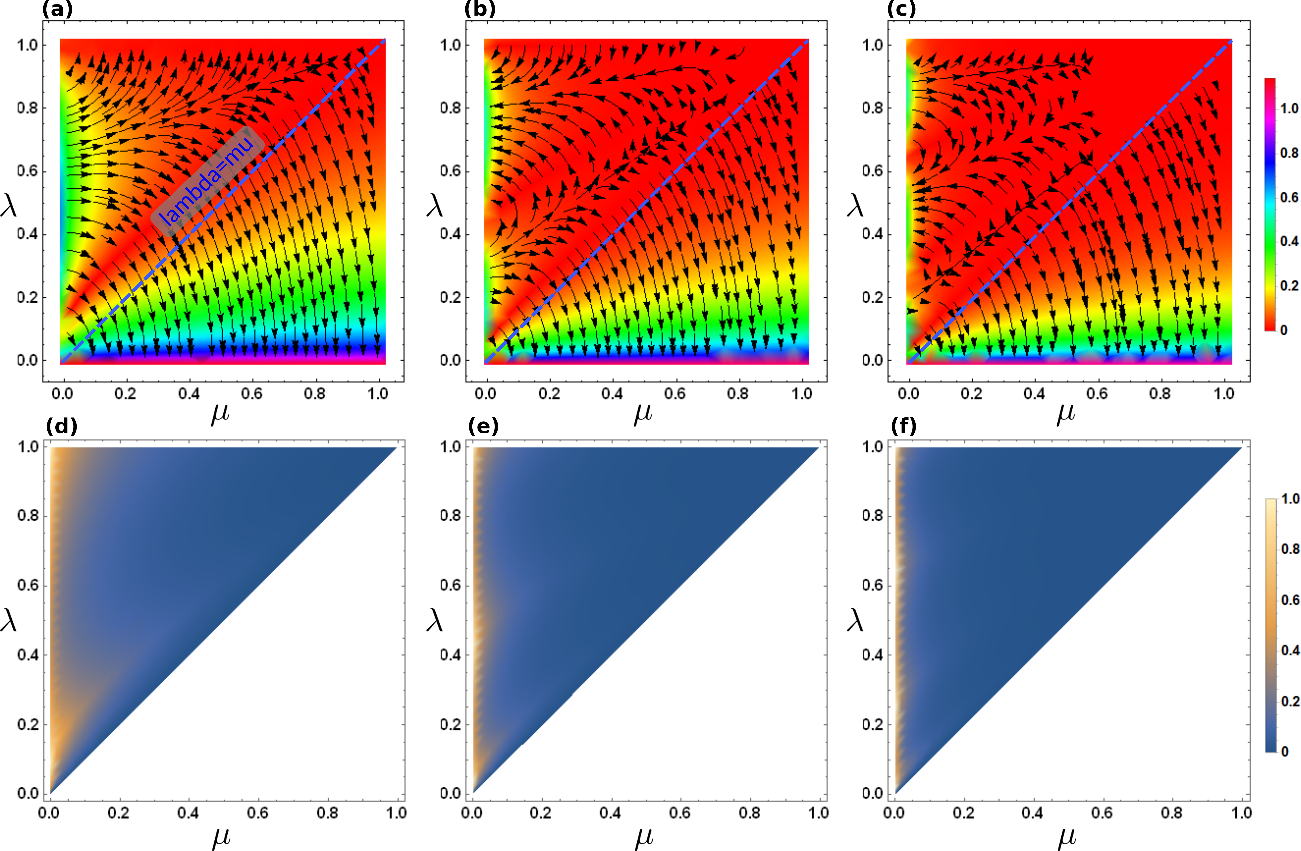
Supplementary Figure 13: Plots used in the derivation of the bounds (187) and (190). (a), (b), and (c) are color density plots of $f_{M}(\mu,\lambda):=\left|1-\sum_{m=0}^{M}{\color[rgb]{1,0,0}{\normalcolor a_{\textrm{Adap},m}^{(M)}}}(\mu)\left(\lambda\right)^{m+1/2}\right|$, for $M=1$, $M=2$, and $M=3$, respectively. The streamlines depict the gradient of $f_{M}(\mu,\lambda)$. In particular, we can see that for $\lambda\leq\mu$ the functions $f_{M}(\mu,\lambda)$ are monotonically decreasing with respect to $\lambda$, and monotonically increasing with respect to $\mu$. The plots (d), (e) and (f) are color density plots of $f_{M}(\mu,\mu)-f_{M}(\mu,\lambda)$ (with $1\leq M\leq 3$ increasing from left to right), for $\lambda\geq\mu$, and show that in this interval $f_{M}(\mu,\mu)\geq f_{M}(\mu,\lambda)$.

on $\varepsilon_{\textrm{KIK}}^{(M)}$, applicable to Taylor error mitigation. While this bound is looser than Eq. (190), it holds for any $M\geq 1$ and not only for $1\leq M\leq 3$. To this end, we apply the Taylor remainder

$$R_{M}(x)=\intop_{a}^{x}\frac{1}{M!}\left(\frac{d^{M+1}f}{dx^{M+1}}\right)_{x=t}(x-t)^{M}dt,$$ (194)

which gives the error $R_{M}(x)=f(x)-P_{M}(x)$ when approximating a function $f(x)$ with the $M$-degree Taylor polynomial

$$P_{M}(x)=\sum_{m=0}^{M}\frac{1}{m!}\left(\frac{d^{m}f}{dx^{m}}\right)_{x=a}(x-a)^{m}.$$ (195)

In Taylor mitigation, we approximate the eigenvalues $f(\lambda)=\lambda^{-\frac{1}{2}}$ of $\left(\mathcal{K}_{\textrm{I}}\mathcal{K}\right)^{-\frac{1}{2}}$, using the Taylor polynomial $P_{M}(\lambda)=\sum_{m=0}^{M}\frac{1}{m!}\left(\frac{(2m-1)!!}{2^{m}}\lambda^{-m-\frac{1}{2}}\right)_{\lambda=1}(\lambda-1)^{m}$. The corresponding Taylor remainder is

$$R_{M}(\lambda)=\intop_{1}^{\lambda}\frac{1}{M!}\frac{(2M+1)!!}{2^{M+1}}t^{-M-\frac{3}{2}}(\lambda-t)^{M}dt.$$ (196)

The eigenvalues of the Hermitian operator $\mathcal{K}_{\textrm{I}}\mathcal{K}=\mathcal{K}^{\dagger}\mathcal{K}$ must satisfy $\lambda\leq 1$. Otherwise, many applications of the evolution $\mathcal{K}_{\textrm{I}}\mathcal{K}$ would lead to a non-physical operation, characterized by divergent eigenvalues. Taking this into account, the absolute value of $R_{M}(\lambda)$ is upper bounded by

$$\left|R_{M}(\lambda)\right| \leq\frac{1}{M!}\frac{(2M+1)!!}{2^{M+1}}\lambda^{-M-\frac{3}{2}}\intop_{\lambda}^{1}\left|(\lambda-t)^{M}\right|dt$$

$$=\frac{1}{M!}\frac{(2M+1)!!}{2^{M+1}}\lambda^{-M-\frac{3}{2}}\intop_{\lambda}^{1}(t-\lambda)^{M}dt$$

$$=\frac{(2M+1)!!}{2^{M+1}(M+1)!}\lambda^{-M-\frac{3}{2}}(1-\lambda)^{M+1}.$$ (197)

Using the diagonal form $\mathcal{K}_{\textrm{I}}\mathcal{K}=\sum_{k}\lambda_{k}|k\rangle\langle k|$, we can express the approximation $\sum_{m=0}^{M}a_{\textrm{Tay},m}^{(M)}\left(\mathcal{K}_{\textrm{I}}\mathcal{K}\right)^{m}$ to the inverse $\left(\mathcal{K}_{\textrm{I}}\mathcal{K}\right)^{-\frac{1}{2}}$ as

$$\sum_{m=0}^{M}a_{\textrm{Tay},m}^{(M)}\left(\mathcal{K}_{\textrm{I}}\mathcal{K}\right)^{m}=\left(\mathcal{K}_{\textrm{I}}\mathcal{K}\right)^{-\frac{1}{2}}+\sum_{k}\left(\pm\left|R_{M}(\lambda_{k})\right|\right)|k\rangle\langle k|.$$ (198)

Therefore,

$$\mathcal{U}_{\textrm{KIK}}^{(M)} =\mathcal{K}\left[\sum_{m=0}^{M}a_{\textrm{Tay},m}^{(M)}\left(\mathcal{K}_{\textrm{I}}\mathcal{K}\right)^{m}\right]$$

$$=\mathcal{U}\left(\mathcal{K}_{\textrm{I}}\mathcal{K}\right)^{\frac{1}{2}}\left[\left(\mathcal{K}_{\textrm{I}}\mathcal{K}\right)^{-\frac{1}{2}}+\sum_{k}\left(\pm\left|R_{M}(\lambda_{k})\right|\right)|k\rangle\langle k|\right]$$

$$=\mathcal{U}+\sum_{k}\left(\pm\lambda_{k}^{\frac{1}{2}}\left|R_{M}(\lambda_{k})\right|\right)|k\rangle\langle k|,$$ (199)

where we write $\mathcal{K}$ as $\mathcal{K}=\mathcal{U}\left(\mathcal{K}_{\textrm{I}}\mathcal{K}\right)^{\frac{1}{2}}$in the second line, and $\left(\mathcal{K}_{\textrm{I}}\mathcal{K}\right)^{\frac{1}{2}}$ as $\left(\mathcal{K}_{\textrm{I}}\mathcal{K}\right)^{\frac{1}{2}}=\sum_{k}\lambda_{k}^{\frac{1}{2}}|k\rangle\langle k|$ in the third line. Accordingly, for Taylor mitigation we have that

$$\varepsilon_{\textrm{KIK}}^{(M)} =\left|\langle A|\left(\mathcal{U}-\mathcal{U}_{\textrm{KIK}}^{(M)}\right)|\rho\rangle\right|$$

$$\leq\frac{(2M+1)!!}{2^{M+1}(M+1)!}\sqrt{\langle A|A\rangle}\left\|\sum_{k}\left(\frac{1}{\lambda_{k}}-1\right)^{M+1}|k\rangle\langle k|\right\|$$

$$=\frac{(2M+1)!!}{2^{M+1}(M+1)!}\sqrt{\langle A|A\rangle}\left(\frac{1}{\textrm{min}_{k}\lambda_{k}}-1\right)^{M+1}$$

$$\leq\frac{(2M+1)!!}{2^{M+1}(M+1)!}\sqrt{\langle A|A\rangle}\left(e^{2\intop_{0}^{T}\left\|\mathcal{L}(t)\right\|dt}-1\right)^{M+1},$$ (200)

where we assume again $\langle\rho|\rho\rangle=1$, and Eqs. (197) and (166) are respectively applied in the second line and the last line.

In the following section, we will take advantage of an important property of the coefficients $a_{\textrm{Adap},m}^{(M)}(\mu)$ and $a_{\textrm{Tay},m}^{(M)}$, in order to further tighten the bounds (187), (190) and (200).

Traceless observables and second (tighter) error bounds for Adaptive error mitigation and Taylor error mitigation. Given an arbitrary observable $A$, we already know that the error-mitigated expectation value in the case of $M$th order mitigation is given by

$$\left\langle A\right\rangle_{\textrm{mit}}=\left\langle A\left|\sum_{m=0}^{M}a_{m}^{(M)}\mathcal{K}\left(\mathcal{K}_{\textrm{I}}\mathcal{K}\right)^{m}\right|\rho\right\rangle,$$ (201)

where $a_{m}^{(M)}=a_{\textrm{Adap},m}^{(M)}(\mu)$ for adaptive mitigation and $a_{m}^{(M)}=a_{\textrm{Tay},m}^{(M)}$ for Taylor mitigation.

Now, let us see that the error $\varepsilon_{\textrm{KIK}}^{(M)}$ is invariant under a transformation $A\rightarrow A+bI$, where $I$ is the identity operator and $b$ is a real number. This shifts the trace of $A$ by the value $b\textrm{Tr}(I)$. Letting $\varepsilon_{\textrm{KIK}}^{(M)}(b)$ denote the error corresponding to the observable $A+bI$, we have that

$$\varepsilon_{\textrm{KIK}}^{(M)}(b) =\left|\left\langle A+bI\left|\sum_{m=0}^{M}a_{m}^{(M)}\mathcal{K}\left(\mathcal{K}_{\textrm{I}}\mathcal{K}\right)^{m}\right|\rho\right\rangle-\left\langle A+bI\left|\mathcal{U}\right|\rho\right\rangle\right|$$

$$=\left|\sum_{m=0}^{M}a_{m}^{(M)}\langle A|\mathcal{K}\left(\mathcal{K}_{\textrm{I}}\mathcal{K}\right)^{m}|\rho\rangle-\left\langle A\left|\mathcal{U}\right|\rho\right\rangle+b\sum_{m=0}^{M}a_{m}^{(M)}-b\right|,$$ (202)

where in the second line we use the fact that $\left\langle I\left|\mathcal{K}\left(\mathcal{K}_{\textrm{I}}\mathcal{K}\right)^{m}\right|\rho\right\rangle=\textrm{Tr}\left(\rho^{(m)}\right)=1$, for a trace-preserving evolution $\mathcal{K}\left(\mathcal{K}_{\textrm{I}}\mathcal{K}\right)^{m}$. Here, $\rho^{(m)}$ is the state resulting from applying the circuit $\mathcal{K}\left(\mathcal{K}_{\textrm{I}}\mathcal{K}\right)^{m}$ on $\rho$.

In the case of adaptive mitigation, we have that, for all $M$, $\sum_{m=0}^{M}a_{m}^{(M)}=\sum_{m=0}^{M}a_{\textrm{Adap},m}^{(M)}(\mu)=1$ by construction. Since in the limit of zero noise the Taylor approximation converges to $\left(\mathcal{K}_{\textrm{I}}\mathcal{K}\right)^{-1}=\mathcal{I}$, it also follows from Eq. (76) that

$$\sum_{m=0}^{M}a_{\textrm{Tay},m}^{(M)}=1,\textrm{ for all }M.$$ (203)

Therefore, Eq. (202) is equivalent to (both for adaptive mitigation and Taylor mitigation)

$$\varepsilon_{\textrm{KIK}}^{(M)}(b)=\varepsilon_{\textrm{KIK}}^{(M)}(0),$$ (204)

for all $b$ real. This result implies that the error $\varepsilon_{\textrm{KIK}}^{(M)}(0)$, associated with the actual observable $A$, can be evaluated using instead the shifted observable $A+bI$. By combining this property with Eqs. (187), (190), and (200), we can obtain the families of $b$-dependent bounds

$$\varepsilon_{\textrm{KIK}}^{(M)}(0) \leq\sqrt{\textrm{Tr}\left[\left(A+bI\right)^{2}\right]}\left|1-\sum_{m=0}^{M}a_{\textrm{Adap},m}^{(M)}(\mu)\left(e^{-2\intop_{0}^{T}\left\|\mathcal{L}(t)\right\|dt}\right)^{m+1/2}\right|,$$ (205)

$$\varepsilon_{\textrm{KIK}}^{(M)}(0) \leq\frac{(2M+1)!!}{2^{M+1}(M+1)!}\sqrt{\textrm{Tr}\left[\left(A+bI\right)^{2}\right]}\left(e^{2\intop_{0}^{T}\left\|\mathcal{L}(t)\right\|dt}-1\right)^{M+1},$$ (206)

where we have written $\langle A+bI|A+bI\rangle$ as $\textrm{Tr}\left[\left(A+bI\right)^{2}\right]$. In the case of Eq. (205), values of $0\leq\mu<1$ yield bounds for adapative mitigation, as per Eq. (187), and $\mu=1$ yields bounds applicable to adaptive mitigation and Taylor mitigation, cf. Eq. (190). On the other hand, Eq. (206) is a consequence of the Taylor-mitigation bound (200).

The tightest bounds in (205) and (206) are obtained by minimizing $\textrm{Tr}\left[\left(A+bI\right)^{2}\right]=\textrm{Tr}\left(A^{2}\right)+2b\textrm{Tr}\left(A\right)+b^{2}\textrm{Tr}\left(I\right)$, with respect to $b$. A simple calculation shows that the minimum is attained by $b$ such that the observable $A+bI$ is traceless, i.e. $\textrm{Tr}\left(A+bI\right)=0$. The resulting expression is

$$b=-\frac{\textrm{Tr}\left(A\right)}{\textrm{Tr}\left(I\right)}.$$ (207)

By substituting this result into Eqs. (205) and (206), we obtain the optimal bounds

$$\varepsilon_{\textrm{KIK}}^{(M)}(0) \leq\sqrt{\textrm{Tr}\left(A^{2}\right)-\frac{\left[\textrm{Tr}\left(A\right)\right]^{2}}{\textrm{Tr}\left(I\right)}}\left|1-\sum_{m=0}^{M}a_{\textrm{Adap},m}^{(M)}(\mu)\left(e^{-2\intop_{0}^{T}\left\|\mathcal{L}(t)\right\|dt}\right)^{m+1/2}\right|,$$ (208)

$$\varepsilon_{\textrm{KIK}}^{(M)}(0) \leq\frac{(2M+1)!!}{2^{M+1}(M+1)!}\sqrt{\textrm{Tr}\left(A^{2}\right)-\frac{\left[\textrm{Tr}\left(A\right)\right]^{2}}{\textrm{Tr}\left(I\right)}}\left(e^{2\intop_{0}^{T}\left\|\mathcal{L}(t)\right\|dt}-1\right)^{M+1}.$$ (209)

Summary. To conclude this supplementary note, we merge the bounds previously derived into a single expression. That is,

$$\varepsilon_{\textrm{KIK}}^{(M)} \leq\sqrt{\textrm{Tr}\left(A^{2}\right)-\frac{\left[\textrm{Tr}\left(A\right)\right]^{2}}{\textrm{Tr}\left(I\right)}}\left|1-\sum_{m=0}^{M}{\color[rgb]{1,0,0}{\normalcolor a_{\textrm{Adap},m}^{(M)}}}(\mu)e^{-2(m+1/2)\intop_{0}^{T}\left\|\mathcal{L}(t)\right\|dt}\right|,\textrm{for }M=1,2,3,$$ (210)

$$\leq\sqrt{\textrm{Tr}\left(A^{2}\right)-\frac{\left[\textrm{Tr}\left(A\right)\right]^{2}}{\textrm{Tr}\left(I\right)}}\left|1-\sum_{m=0}^{M}{\color[rgb]{1,0,0}{\normalcolor a_{\textrm{Adap},m}^{(M)}}}(1)e^{-2(m+1/2)\intop_{0}^{T}\left\|\mathcal{L}(t)\right\|dt}\right|,\textrm{{for }}M=1,2,3,$$ (211)

$$\leq\frac{(2M+1)!!}{2^{M+1}(M+1)!}\sqrt{\textrm{Tr}\left(A^{2}\right)-\frac{\left[\textrm{Tr}\left(A\right)\right]^{2}}{\textrm{Tr}\left(I\right)}}\left(e^{2\intop_{0}^{T}\left\|\mathcal{L}(t)\right\|dt}-1\right)^{M+1},$$ (212)

where Eq. (210) is equivalent to Eq. (208), and (211) follows by applying the optimization strategy of the previous section to Eq. (190). Equation (212) corresponds to Eq. (209), and is the looser bound according to Supplementary Figure 14. We also recall that the bound (211) is valid for both adaptive mitigation and Taylor mitigation, in addition to being independent of $\mu$. On the other hand, the bound (212) is valid for Taylor mitigation and for all $M\geq 1$. From this bound we can also see that the error $\varepsilon_{\textrm{KIK}}^{(M)}$ is exponentially decreasing in $M$ if $\intop_{0}^{T}\left\|\mathcal{L}(t)\right\|dt<\frac{1}{2}\textrm{ln}(2)$, since the prefactor $\frac{(2M+1)!!}{2^{M+1}(M+1)!}$ satisfies $\frac{(2M+1)!!}{2^{M+1}(M+1)!}\leq\frac{3}{8}$.

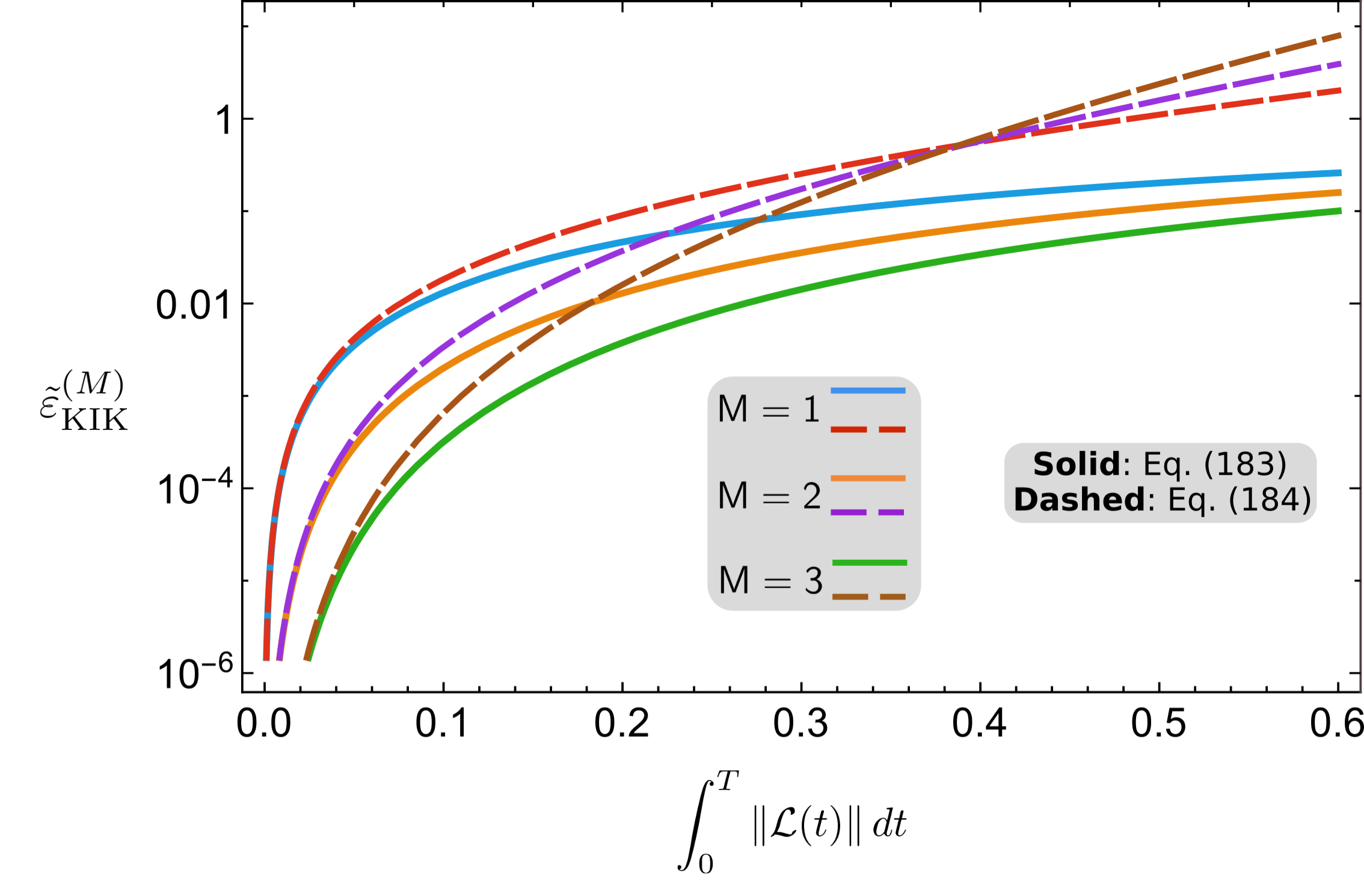
Supplementary Figure 14: Upper bounds (211) and (212) on $\tilde{\varepsilon}_{\textrm{KIK}}^{(M)}:=\frac{\varepsilon_{\textrm{KIK}}^{(M)}}{\sqrt{\textrm{Tr}\left(A^{2}\right)-\frac{\left[\textrm{Tr}\left(A\right)\right]^{2}}{\textrm{Tr}\left(I\right)}}}$, for mitigation orders $M=1,2,3$.

We also stress that, once coherent noise is converted into incoherent noise, via RC, the quantity $\intop_{0}^{T}\left\|\mathcal{L}(t)\right\|dt$ accounts for the total error rate affecting the evolution $\mathcal{K}$, irrespective of the depth or the width of the corresponding circuit. Therefore, the bounds (210)-(212) are meaningful to assess the performance of the KIK method applied to circuits $\mathcal{K}$ of arbitrary size. It is also important to note that generic QEM methods can be useful so long as the total error rate is not excessively high ²². In the context of the KIK method, we can have scalable QEM if $\intop_{0}^{T}\left\|\mathcal{L}(t)\right\|dt$ is kept below a fixed value for increasingly large circuits, and if for this value the bound (210) is sufficiently small.

References

- (1) Arute, F. et al. Quantum supremacy using a programmable superconducting processor. Nature 574, 505–510 (2019).
- (2) Zhong, H.-S. et al. Quantum computational advantage using photons. Science 370, 1460–1463 (2020).
- (3) Madsen, L. S. et al. Quantum computational advantage with a programmable photonic processor. Nature 606, 75–81 (2022).
- (4) Fowler, A. G., Mariantoni, M., Martinis, J. M. & Cleland, A. N. Surface codes: Towards practical large-scale quantum computation. Phys. Rev. A 86, 032324 (2012).
- (5) O Gorman, J. & Campbell, E. T. Quantum computation with realistic magic-state factories. Phys. Rev. A 95, 032338 (2017).
- (6) Temme, K., Bravyi, S. & Gambetta, J. M. Error mitigation for short-depth quantum circuits. Phys. Rev. Lett. 119, 180509 (2017).
- (7) Li, Y. & Benjamin, S. C. Efficient variational quantum simulator incorporating active error minimization. Phys. Rev. X 7, 021050 (2017).
- (8) Endo, S., Benjamin, S. C. & Li, Y. Practical quantum error mitigation for near-future applications. Phys. Rev. X 8, 031027 (2018).
- (9) Strikis, A., Qin, D., Chen, Y., Benjamin, S. C. & Li, Y. Learning-based quantum error mitigation. PRX Quantum 2, 040330 (2021).
- (10) Czarnik, P., Arrasmith, A., Coles, P. J. & Cincio, L. Error mitigation with clifford quantum-circuit data. Quantum 5, 592 (2021).
- (11) Koczor, B. Exponential error suppression for near-term quantum devices. Phys. Rev. X 11, 031057 (2021).
- (12) Huggins, W. J. et al. Virtual distillation for quantum error mitigation. Phys. Rev. X 11, 041036 (2021).
- (13) Giurgica-Tiron, T., Hindy, Y., LaRose, R., Mari, A. & Zeng, W. J. Digital zero noise extrapolation for quantum error mitigation. In 2020 IEEE International Conference on Quantum Computing and Engineering (QCE), 306–316 (IEEE, 2020).
- (14) Cai, Z. Quantum error mitigation using symmetry expansion. Quantum 5, 548 (2021).
- (15) Mari, A., Shammah, N. & Zeng, W. J. Extending quantum probabilistic error cancellation by noise scaling. Phys. Rev. A 104, 052607 (2021).
- (16) Lowe, A. et al. Unified approach to data-driven quantum error mitigation. Phys. Rev. Research 3, 033098 (2021).
- (17) Nation, P. D., Kang, H., Sundaresan, N. & Gambetta, J. M. Scalable mitigation of measurement errors on quantum computers. PRX Quantum 2, 040326 (2021).
- (18) Bravyi, S., Sheldon, S., Kandala, A., Mckay, D. C. & Gambetta, J. M. Mitigating measurement errors in multiqubit experiments. Phys. Rev. A 103, 042605 (2021).
- (19) Kim, Y. et al. Scalable error mitigation for noisy quantum circuits produces competitive expectation values. Nat. Phys. 1–8 (2023).
- (20) Van Den Berg, E., Minev, Z. K., Kandala, A. & Temme, K. Probabilistic error cancellation with sparse pauli–lindblad models on noisy quantum processors. Nat. Phys. 19, 1–2 (2023).
- (21) Ferracin, S. et al. Efficiently improving the performance of noisy quantum computers. Preprint at https://arxiv.org/abs/2201.10672 (2022).
- (22) Endo, S., Cai, Z., Benjamin, S. C. & Yuan, X. Hybrid quantum-classical algorithms and quantum error mitigation. J. Phys. Soc. Jpn. 90, 032001 (2021).
- (23) Cai, Z. et al. Quantum error mitigation. Preprint at https://arxiv.org/abs/2210.00921v2 (2022).
- (24) Kandala, A. et al. Error mitigation extends the computational reach of a noisy quantum processor. Nature 567, 491–495 (2019).
- (25) Song, C. et al. Quantum computation with universal error mitigation on a superconducting quantum processor. Sci. Adv. 5, eaaw5686 (2019).
- (26) Quantum, G. A. et al. Hartree-fock on a superconducting qubit quantum computer. Science 369, 1084–1089 (2020).
- (27) Urbanek, M. et al. Mitigating depolarizing noise on quantum computers with noise-estimation circuits. Phys. Rev. Lett. 127, 270502 (2021).
- (28) Kim, Y. et al. Evidence for the utility of quantum computing before fault tolerance. Nature 618, 500–505 (2023).
- (29) Shtanko, O. et al. Uncovering local integrability in quantum many-body dynamics. Preprint at https://arxiv.org/abs/2307.07552 (2023).
- (30) Zhang, S. et al. Error-mitigated quantum gates exceeding physical fidelities in a trapped-ion system. Nat. Commun. 11, 587 (2020).
- (31) Sagastizabal, R. et al. Experimental error mitigation via symmetry verification in a variational quantum eigensolver. Phys. Rev. A 100, 010302 (2019).
- (32) Wallman, J. J. & Emerson, J. Noise tailoring for scalable quantum computation via randomized compiling. Phys. Rev. A 94, 052325 (2016).
- (33) Hashim, A. et al. Randomized compiling for scalable quantum computing on a noisy superconducting quantum processor. Phys. Rev. X 11, 041039 (2021).
- (34) Majumdar, R., Rivero, P., Metz, F., Hasan, A. & Wang, D. S. Best practices for quantum error mitigation with digital zero-noise extrapolation. Preprint at https://arxiv.org/abs/2307.05203 (2023).
- (35) Czarnik, P., McKerns, M., Sornborger, A. T. & Cincio, L. Improving the efficiency of learning-based error mitigation. Preprint at https://arxiv.org/abs/2204.07109 (2022).
- (36) Takagi, R., Endo, S., Minagawa, S. & Gu, M. Fundamental limits of quantum error mitigation. npj Quantum Inf. 8, 114 (2022).
- (37) Quek, Y., França, D. S., Khatri, S., Meyer, J. J. & Eisert, J. Exponentially tighter bounds on limitations of quantum error mitigation. Preprint at https://arxiv.org/abs/2210.11505 (2022).
- (38) Trotter, H. F. On the product of semi-groups of operators. Proc. Amer. Math. Soc. 10, 545–551 (1959).
- (39) Gyamfi, J. A. Fundamentals of quantum mechanics in liouville space. Eur. J. Phys. 41, 063002 (2020).
- (40) Blanes, S., Casas, F., Oteo, J.-A. & Ros, J. The magnus expansion and some of its applications. Phys. Rep. 470, 151–238 (2009).
- (41) Breuer, H.-P. & Petruccione, F. The theory of open quantum systems (Oxford University Press, 2002).
- (42) Sun, J. et al. Mitigating realistic noise in practical noisy intermediate-scale quantum devices. Phys. Rev. Applied 15, 034026 (2021).
- (43) López, J. L. & Temme, N. M. Two-point taylor expansions of analytic functions. Studies in Applied Mathematics 109, 297–311 (2002).
- (44) Landa, H., Meirom, D., Kanazawa, N., Fitzpatrick, M. & Wood, C. J. Experimental bayesian estimation of quantum state preparation, measurement, and gate errors in multiqubit devices. Phys. Rev. Research 4, 013199 (2022).
- (45) Alexander, T. et al. Qiskit pulse: programming quantum computers through the cloud with pulses. Quantum Sci. Technol. 5, 044006 (2020).
- (46) He, A., Nachman, B., de Jong, W. A. & Bauer, C. W. Zero-noise extrapolation for quantum-gate error mitigation with identity insertions. Phys. Rev. A 102, 012426 (2020).
- (47) Pascuzzi, V. R., He, A., Bauer, C. W., de Jong, W. A. & Nachman, B. Computationally efficient zero-noise extrapolation for quantum-gate-error mitigation. Phys. Rev. A 105, 042406 (2022).
- (48) Dann, R., Levy, A. & Kosloff, R. Time-dependent markovian quantum master equation. Phys. Rev. A 98, 052129 (2018).
- (49) Jnane, H., Undseth, B., Cai, Z., Benjamin, S. C. & Koczor, B. Multicore quantum computing. Phys. Rev. Applied 18, 044064 (2022).
- (50) Nielsen, M. A. & Chuang, I. Quantum computation and quantum information (American Association of Physics Teachers, 2002).
- (51) Wallman, J., Granade, C., Harper, R. & Flammia, S. T. Estimating the coherence of noise. New J. Phys. 17, 113020 (2015).
- (52) Zhang, B. et al. Hidden inverses: Coherent error cancellation at the circuit level. Phys. Rev. Applied 17, 034074 (2022).
- (53) Greenbaum, D. Introduction to quantum gate set tomography. Preprint at https://arxiv.org/abs/1509.02921 (2015).