Kernel Free Boundary Integral Method for 3D Stokes and Navier Equations on Irregular Domains

Abstract

A second-order accurate kernel-free boundary integral method is presented for Stokes and Navier boundary value problems on three-dimensional irregular domains. It solves equations in the framework of boundary integral equations, whose corresponding discrete forms are well-conditioned and solved by the GMRES method. A notable feature of this approach is that the boundary or volume integrals encountered in BIEs are indirectly evaluated by a Cartesian grid-based method, which includes discretizing corresponding simple interface problems with a MAC scheme, correcting discrete linear systems to reduce large local truncation errors near the interface, solving the modified system by a CG method together with an FFT-based Poisson solver. No extra work or special quadratures are required to deal with singular or hyper-singular boundary integrals and the dependence on the analytical expressions of Green’s functions for the integral kernels is completely eliminated. Numerical results are given to demonstrate the efficiency and accuracy of the Cartesian grid-based method.

1 Introduction

The Stokes and Navier problems are two important models constructed in incompressible fluid and solid mechanics, and have wide applications in engineering and sciences, such as lubrication theory [32], porous media flow [23], tissue engineering [40], biomedical science [41] and so on. Therefore, it is always of great interest to find simple, effective and robust numerical schemes for solving these models.

For such problems defined on irregular or complex geometries, a traditional numerical method such as the finite element method (FEM) with a body-fitted grid suffers from a major challenge on efficient mesh generation and accurate solution of corresponding systems. Especially in three dimensions or when moving boundaries are involved, mesh generation and re-meshing become difficult and time-consuming. In addition, another difficulty is the design of robust and fast solvers for the resulting discrete equations. Although multilevel techniques such as multi-grid or domain decomposition have been extended to unstructured grids, vector PDEs or indefinite operators like the Stokes equations have not been widely applied.

Also, many numerical methods, such as the finite difference method, do not naturally apply to unstructured meshes. In order to avoid these drawbacks, the use of Cartesian grid-based methods has become quite widespread. Representative numerical methods of this type partially include immersed boundary method (IBM) [29], immersed interface method (IIM) [24], CutFEM [15], extended finite element method (XFEM)[7], Nitsche’s XFEM [38], immersed finite element method (IFEM) [16], matched interface and boundary (MIB) method [50] and so on. To maintain the desired accuracy, techniques such as smoothing or regularization of discontinuities, correction of the discretization schemes and modification of the approximation functions or basis are usually employed. Most Cartesian grid-based methods enable one to employ much simple meshes, but in some cases, fast methods are not straightforward to apply.

Boundary integral methods (BIMs) have been used most extensively in the case of ellipses because they have the significant advantages of handling complex or irregular domains and using fast algorithms to dramatically decrease the computational cost. The main idea is to embed the complex or irregular domain into a larger regular domain, and then the boundary value problems can be reformulated into Fredholm BIEs of the second kind, which leads to the fact that only the domain boundary or surface is needed to be partitioned, thus avoiding the generation of high-quality boundary-fitted mesh on irregular domains, and considerably reducing the dimensionality of unknowns in the solution. After the first numerical implementation of the boundary integral formulation for Stokes flow reported by Youngren and Acrivos in [48], BIMs have played an important role in fluid mechanics, elasticity and other application areas [12, 19, 30, 1, 49, 14, 4]. However, there exist several potential practical issues that have prevented the broad application of approaches of this type. For example, the singularities of the fundamental solution can involve increased computational costs and implementation complexity when computing the near field interaction. Although various fast techniques have been developed to speed up the calculation of singular integrals (see e.g.[18, 3, 21, 35] and references therein for further information), it is still an active research topic. In addition, the unavailability of the analytical expression of the kernel functions also restricts the traditional BIMs to the constant coefficients boundary value problems in the free space subject to the far field radiation condition or in a rectangle domain subject to the periodic boundary condition.

For these reasons, a different approach has emerged. This method, referred to as Kernel-free boundary integral (KFBI) method, is a generalization of the traditional BIMs, particularly the grid-based BIM by Mayo et al. [26, 27, 28] and J.T.Beale et al [2]. It evaluates boundary and volume integrals indirectly by a Cartesian grid-based method, thus possessing the following two most prominent features: i) it does not require the explicit expressions of Green’s function or special quadratures formulas to directly calculate integrals, especially nearly singular or hyper-singular boundary integrals, so that the dependence on the kernel can be completely eliminated in practice; ii) it reformulates the boundary value problems as the Fredholm BIE of the second kind, helping to eliminate the ill-conditioning property of the original problems so that the number of Krylov subspace iterations is essentially independent of the discretization parameter or system dimension. The KFBI method has been developed to be a general method for two-dimensional elliptic PDEs [45, 46, 47, 44, 42, 43, 6], but for three-dimensional problems, it is now under intensive development.

This work extends the KFBI method to solve Stokes and Navier equations in three-dimensional irregular domains. Based on potential theory, the solution of a Dirichlet problem is written as the sum of a volume integral and a double-layer boundary integral with an unknown density. These integrals are evaluated indirectly by a Cartesian grid-based method, which primarily consists of two steps: (1) solving corresponding equivalent but simple interface problems in an extended cubic region, (2) extracting the boundary value of the integrals by a procedure of polynomial interpolation. During the calculation, the equivalent Stokes and Navier interface problems are discretized in a uniform mixed formulation with a modified MAC Scheme, generalized slightly by allowing a pressure term in the continuity equation. The resulting linear system is solved efficiently by the CG method together with an FFT-based Poisson solver. The Cartesian grid-based indirect evaluation technique has the superiorities of requiring no extra work or special quadratures to handle singular or hyper-singular boundary integrals without the need to analytical expressions of Green’s functions for the integral kernels.

In addition, no unstructured triangulation of the surface is required in the KFBI method. It only uses some quasi-uniform control points, which are represented by intersection points of the surface with an underlying Cartesian grid, to discretize the density and the boundary integral equations. Such a selection of control points makes the interpolation stencils in the integral evaluation convenient to choose and locally uniform on a coordinate plane in three space dimensions. As the intersection points of an implicit surface with Cartesian grid line can be found straightforwardly in three space dimensions, it is very easy to implement the algorithm. These attributes have special importance for the time-dependent problems with moving boundaries. Numerical results show that the KFBI method is efficient and accurate in handling incompressible fluid and solid mechanics problems on irregular domains.

The remainder of this article is organized as follows. In section 2, the Stokes and Navier problems are described respectively. The main idea of the KFBI algorithm is given in section 3. The essential implementation details for integral evaluation are given in section 4. In section 5, numerical results are provided to validate the effectiveness of the proposed method. Concluding remarks and some discussions are put in section 6.

2 Boundary Value Problems

Let $\Omega\in\mathbb{R}^{3}$ be a bounded domain with smooth boundary $\partial\Omega$, which is in general irregular and complex. The steady-state incompressible Stokes equations considered in this work are given by

$$-\mu_{s}\Delta{\bf u}_{s}+\nabla p_{s} ={\bf f}_{s},\quad\,\hbox{in}\;\Omega,$$ (1a)

$$\nabla\cdot{\bf u}_{s} =0,\quad\;\,\hbox{in}\;\Omega,$$ (1b)

$${\bf u}_{s} ={\bf g}_{s},\quad\hbox{on}\;\partial\Omega,$$ (1c)

where ${\bf u}_{s}=(u^{(1)}_{s},u^{(2)}_{s},u^{(3)}_{s})^{T}$ stands for the velocity vector, $p_{s}$ represents the pressure, $\mu_{s}$ is the fluid viscosity coefficient, ${\bf f}_{s}=(f_{s}^{(1)},f_{s}^{(2)},f_{s}^{(3)})^{T}$ denotes an external force and ${\bf g}_{s}=(g_{s}^{(1)},g_{s}^{(2)},g_{s}^{(3)})^{T}$ is the Dirichlet-type boundary condition of ${\bf u}_{s}$ on the boundary $\partial\Omega$. Assume that $\mu_{s}$ is a constant function on $\Omega$ and ${\bf g}_{s}$ satisfies the compatibility condition

$$\int_{\partial\Omega}{\bf g}_{s}\cdot{\bf n}ds=0,$$

where ${\bf n}$ denotes the unit outward normal vector on $\partial\Omega$. The 3D Navier equations are also considered here, which are governed by

$$\nabla\cdot\boldsymbol{\sigma}({\bf u}_{e})+{\bf f}_{e} ={\bf 0},\,\;\;\quad{\rm in}\;\Omega,$$ (2a)

$${\bf u}_{e} ={\bf g}_{e},\;\quad{\rm on}\;\partial\Omega,$$ (2b)

where ${\bf u}_{e}=(u^{(1)}_{e},u^{(2)}_{e},u^{(3)}_{e})^{T}$ is the displacement field, ${\bf f}_{e}=(f^{(1)}_{e},f^{(2)}_{e},f^{(3)}_{e})^{T}$ is a given body force, ${\bf g}_{e}=(g^{(1)}_{e},g^{(2)}_{e},g^{(3)}_{e})^{T}$ represents the displacement on the boundary. The stress tensor is given by

$$\boldsymbol{\sigma}({\bf u}_{e})=\lambda\nabla\cdot{\bf u}_{e}{\bf I}+2\mu\boldsymbol{\epsilon}({\bf u}_{e}),$$ (3)

where $\boldsymbol{\epsilon}({\bf u}_{e})=\dfrac{1}{2}\big{(}\nabla{\bf u}_{e}+(\nabla{\bf u}_{e})^{T}\big{)}$ is the linear strain and ${\bf I}$ is the $3\times 3$ identical matrix. Furthermore, $\lambda$ and $\mu$ represent the Lamé coefficients, satisfying

$$\lambda=\dfrac{E\nu}{(1+\nu)(1-2\nu)},\hbox{\qquad and \qquad}\mu=\dfrac{E}{2(1+\nu)},$$

with $E$ the Young’s modulus and $\nu$ the Poisson’s ratio. By inserting the strain tensor (3) into the equilibrium equation (2a), the 3D Navier problem can be reformulated as a system of partial differential equations where the unknown function is the displacement field ${\bf u}_{e}$:

$$-\mu\Delta{\bf u}_{e}-(\lambda+\mu)\nabla(\nabla\cdot{\bf u}_{e})={\bf f}_{e},\;\;\hbox{in}\;\Omega.$$ (4)

3 The Kernel Free Boundary Integral Method

This section gives details of the Cartesian grid-based KFBI method for solving Stokes and Navier problems in three-dimensional irregular domains.

To this end, the irregular domain $\Omega$ is embedded into a larger cube $\mathcal{B}$, thus the domain boundary becomes an interface, which separates the cuboid into two disconnected subdomains $\Omega$ and $\Omega^{c}$. Here, $\Omega^{c}=\mathcal{B}\backslash\bar{\Omega}$ is the complement of $\Omega$ in $\mathcal{B}$. In the remainder of this article, the boundary $\partial\Omega$ is redefined as $\Gamma$. Next, problems (1) and (2) will be reformulated into boundary integral equations respectively. Let $({\bf G}_{{\bf v}}({\bf x},{\bf y}),G_{q}({\bf x},{\bf y}))$ be Green’s function pair associated with the Stokes equation (1) that satisfies

$$\begin{split}-\mu_{s}\Delta{\bf G}_{{\bf v}}({\bf x},{\bf y})+\nabla G_{q}({\bf x},{\bf y})&={\bf I}\delta({\bf x}-{\bf y}),\quad\hbox{in}\;\mathcal{B},\\ \nabla\cdot{\bf G}_{{\bf v}}({\bf x},{\bf y})&=0,\qquad\qquad\;\;\,\hbox{in}\;\mathcal{B},\\ {\bf G}_{{\bf v}}({\bf x},{\bf y})&={\bf 0},\qquad\qquad\;\;\hbox{on}\;\partial\mathcal{B},\end{split}$$ (5)

for each fixed ${\bf y}\in\mathcal{B}$. Let ${\bf G}({\bf x},{\bf y})$ be Green’s function associated with Navier system (2) that satisfies

$$\begin{split}-\mu\Delta{\bf G}({\bf x},{\bf y})-(\lambda+\mu)\nabla\big{(}\nabla\cdot{\bf G}({\bf x},{\bf y})\big{)}&={\bf I}\delta({\bf x}-{\bf y}),\;\;\;{\rm in}\;\mathcal{B},\\ {\bf G}({\bf x},{\bf y})&={\bf 0},\qquad\,\qquad\;{\rm on}\;\partial\mathcal{B},\end{split}$$ (6)

for each fixed ${\bf y}\in\mathcal{B}$. Here, the matrix ${\bf I}$ denotes the unit matrix in $\mathbb{R}^{3}$ and $\delta({\bf x}-{\bf y})$ is the 3D Dirac delta function. All differentiations are carried out with respect to the variable ${\bf x}$. It is important to point out that the Green’s function pair $({\bf G}_{{\bf v}}({\bf x},{\bf y}),G_{q}({\bf x},{\bf y}))$ and Green’s function ${\bf G}({\bf x},{\bf y})$ defined in the bounded domain $\mathcal{B}$ are different from the fundamental solution in the free space [17]. Their expressions are in general not analytically known, but their existence is guaranteed.

In terms of the Green’s function pair $({\bf G}_{{\bf v}},G_{q})$, the solutions ${\bf u}_{s}({\bf x})$ and $p_{s}({\bf x})$ to the Stokes problem (1) can be expressed as a sum of the double layer potential and volume integral

$${\bf u}_{s}({\bf x})=\mathcal{G}_{{\bf v}}{\bf f}_{s}({\bf x})-\mathcal{M}_{{\bf v}}\boldsymbol{\varphi}_{s}({\bf x}),\quad{\bf x}\in\Omega,$$ (7)

$$\,p_{s}({\bf x})=\mathcal{G}_{q}{\bf f}_{s}({\bf x})-\mathcal{M}_{q}\boldsymbol{\varphi}_{s}({\bf x}),\;\quad{\bf x}\in\Omega,$$ (8)

with density $\boldsymbol{\varphi}_{s}({\bf x})$ satisfying the boundary integral equation

$$\begin{split}\frac{1}{2}\boldsymbol{\varphi}_{s}({\bf x})-\mathcal{M}_{{\bf v}}\boldsymbol{\varphi}_{s}({\bf x})={\bf g}_{s}({\bf x})-\mathcal{G}_{{\bf v}}{\bf f}_{s}({\bf x}),\qquad{\bf x}\in\Gamma.\end{split}$$ (9)

Here, the double layer boundary integrals $\mathcal{M}_{{\bf v}}\boldsymbol{\varphi}_{s}$, $\mathcal{M}_{q}\boldsymbol{\varphi}_{s}$ and volume integrals $\mathcal{G}_{{\bf v}}{\bf f}_{s}$, $\mathcal{G}_{q}{\bf f}_{s}$ are given respectively by

$$\begin{split}(\mathcal{M}_{{\bf v}}\boldsymbol{\varphi}_{s})({\bf x})&=\int_{\Gamma}T_{s}({\bf G}_{{\bf v}},G_{q})\boldsymbol{\varphi}_{s}({\bf y})ds_{{\bf y}},\quad\;\;(\mathcal{G}_{{\bf v}}{\bf f}_{s})({\bf x})=\int_{\Omega}{\bf G}_{{\bf v}}({\bf x},{\bf y}){\bf f}_{s}({\bf y})d{\bf y},\\ (\mathcal{M}_{q}\boldsymbol{\varphi}_{s})({\bf x})&=2\int_{\Gamma}\dfrac{\partial G_{q}({\bf x},{\bf y})}{\partial{\bf n}_{{\bf y}}}\boldsymbol{\varphi}_{s}({\bf y})ds_{{\bf y}},\quad(\mathcal{G}_{q}{\bf f}_{s})({\bf x})=\int_{\Omega}G_{q}({\bf x},{\bf y})\cdot{\bf f}_{s}({\bf y})d{\bf y},\end{split}$$

with the traction ${\bf T}_{s}({\bf u}_{s},p_{s})=-p_{s}{\bf n}+\mu(\nabla{\bf u}_{s}+\nabla{\bf u}_{s}^{T}){\bf n}.$ Similarly, in terms of Green’s function ${\bf G}({\bf x},{\bf y})$, the solution ${\bf u}_{e}$ to the Navier equations (2) can also be expressed as a sum of the double layer potential and volume integral

$${\bf u}_{e}({\bf x})=\mathcal{G}{\bf f}_{e}({\bf x})-\mathcal{M}\boldsymbol{\varphi}_{e}({\bf x}),\quad{\bf x}\in\Omega,$$ (10)

with density $\boldsymbol{\varphi}_{e}({\bf x})$ satisfying the boundary integral equation

$$\frac{1}{2}\boldsymbol{\varphi}_{e}({\bf x})-\mathcal{M}\boldsymbol{\varphi}_{e}({\bf x})={\bf g}_{e}({\bf x})-\mathcal{G}{\bf f}_{e}({\bf x}).$$ (11)

Here, the double layer boundary integral $\mathcal{M}\boldsymbol{\varphi}_{e}$ and volume integral $\mathcal{G}{\bf f}_{e}$ are defined respectively by

$$(\mathcal{M}\boldsymbol{\varphi}_{e})({\bf x})=\int_{\Gamma}{\bf T}_{{\bf y}}\boldsymbol{G}({\bf x},{\bf y})\boldsymbol{\varphi}_{e}({\bf y})ds_{{\bf y}},\qquad(\mathcal{G}{\bf f}_{e})({\bf x})=\int_{\Omega}{\bf G}({\bf x},{\bf y}){\bf f}_{e}({\bf y})d{\bf y},$$ (12)

with the traction defined by

$${\bf T}({\bf u}_{e})=\lambda(\nabla\cdot{\bf u}_{e}){\bf n}+2\mu\dfrac{\partial{\bf u}_{e}}{\partial{\bf n}}+\mu{\bf n}\times(\nabla\times{\bf u}_{e}).$$

It is pointed out that the subscript ${\bf y}$ in ${\bf T}_{{\bf y}}{\bf G}({\bf x},{\bf y})$ denotes the differentiations in (12) with respect to the variable ${\bf y}$. Note that the BIEs (9) and (11) are Fredholm integral equations of the second kind [22], which indicate that the iterative methods, such as the generalized minimal residual (GMRES) method[31], or even the simple Richardson iteration, converge for each ${\bf g}_{s}/{\bf g}_{e}$ and initial data $\boldsymbol{\varphi}_{s}^{0}/\boldsymbol{\varphi}_{e}^{0}$ to the unique solution of (9) or (11).

Once the iteration converges, one can get approximation of ${\bf u}_{s}$ or ${\bf u}_{e}$ respectively according to the representation formula (7) and (10). As the Green’s function pair $({\bf G}_{{\bf v}},G_{q})$ and Green’s function ${\bf G}$ are defined in a bounded domain $\mathcal{B}$, their analytical expressions are un-available, thus it is impossible to directly calculate the boundary and volume integrals encountered in BIEs (9) and (11).

For this reason, a Cartesian grid-based KFBI method that calculates integrals indirectly is adopted here, so it is not necessary to know the analytical expression of Green’s function. The main idea of KFBI consists three main steps: 1) The irregular domain $\Omega$ is embedded into a larger cuboid area $\mathcal{B}$, which is easy to obtain a uniform Cartesian grid, thus avoids generating unstructured grids for complex domains effectively. Then the boundary value problems (1)-(2) are reformulated into Fredholm BIEs of the second kind (9) and (11). 2) Evaluation of the integrals encountered in the BIEs are made indirectly by a Cartesian grid-based method, including discretizing the corresponding interface problem with a MAC scheme, correcting the established linear system to reduce the large local truncation errors near the interface, solving the modified system by a CG method together with the FFT-based Poisson solvers, approximating values of the integrals or its normal flux on the interface by quadratic polynomial interpolation. 3) The BIEs are well-conditioned and the corresponding discrete form can be solved efficiently with a Krylov subspace method, such as the GMRES method, with the number of iterations independent of the mesh size. At last, the algorithm is summarized as follows:

Algorithm 1 KFBI method for 3D Stokes and Navier Equations.

Find quasi-uniform control points to discretize BIEs.

• Set up five different uniform staggered grids with size $h$ covering larger cuboid area $\mathcal{B}$.

• Each grid point is marked as an interior or exterior point according to the interface.

• Identify regular and irregular grid nodes of the uniform grids.

• Find the intersection points of the boundary and the grid lines, and compute tangential and normal unit directions of the boundary curve at those intersected points.

Evaluate the boundary or volume integral at the boundary $\Gamma$.

• Write the equivalent interface problems of Navier and Stokes as a unified form by introducing an auxiliary unknown pressure.

• Discretize the equivalent interface problems with a finite-difference-based MAC scheme.

• Compute jumps of the solutions and their partial derivatives at intersection points.

• Correct the right-hand side of the MAC scheme at irregular grid nodes.

• Solve the modified linear system by the CG method together with an FFT-based Poisson solver.

• Extract the boundary data at intersected points by quadratic polynomial interpolation.

Make the GMRES iteration with the KFBI method.

• Evaluate the volume integral boundary data with step 2.

• Start the GMRES iteration with the trivial zero initial guess and set up a tolerance.

• Evaluate the double layer integral boundary data with step 2.

• Update the unknown density $\boldsymbol{\varphi}_{s}$ by the GMRES iteration until the residual is smaller than the prescribed tolerance in some norm.

Noted that the points used to represent the boundary and discretize the BIE are chosen as intersection points of the boundary surface with the grid lines of the underlying staggered grid, which was originally prescribed in [46] by Wenjun Ying and Wei-Cheng Wang. With this technique, the discretization points are convenient to locate. Moreover, the points are classified as the primary and secondary points and each of them is associated with a component of boundary data during the solution of the BIE, which makes it easy to find out compact and locally uniform interpolation stencils for boundary interpolation. And an additional equilibration process further ensures the stability and efficiency of the numerical differentiation when calculating the tangential derivatives of the boundary. One may refer to the reference [46] for a detailed presentation.

The main challenge in the above algorithm is the evaluation of integrals appeared in BIEs, as the conceivable unavailability of the analytical expressions of Green’s functions. To this end, each boundary and volume integral is calculated by interpolating structured grid-based solutions, which avoids directly discretizing the integrals by numerical quadratures, so that the dependence on the analytical expressions of Green’s functions can be completely eliminated in implementation. Details of the evaluation are presented in the ensuing sections.

4 Evaluation of Boundary or Volume Integrals

In this section, a Cartesian grid-based method for indirectly evaluating boundary and volume integrals is presented. In this method, analytical expressions of Green’s functions are no longer needed and the integrals are calculated indirectly through the following steps :

• transforming the boundary or volume integral into equivalent interface problems;

• solving the equivalent but simple interface problem under Cartesian mesh;

• interpolating the discrete solution on the Cartesian mesh to extract values of the integrals at discretization points of the interface.

4.1 Equivalent Simple Interface Problems

The equivalent simple interface problems for the volume and double layer boundary integrals will be illustrated here, respectively. Let ${\bf v}^{+}({\bf x})$ and ${\bf v}^{-}({\bf x})$ be the restrictions of ${\bf v}({\bf x})$ from the subdomain $\Omega$ and $\Omega^{c}$. For ${\bf x}\in\Gamma$, ${\bf v}^{+}({\bf x})$ and ${\bf v}^{-}({\bf s})$ are interpreted as the limit values of ${\bf v}({\bf x})$ from the corresponding side of the domain boundary. The jump across the interface $\Gamma$ is denoted by

$$\begin{split}[\![{\bf v}({\bf x})]\!]={\bf v}^{+}({\bf x})-{\bf v}^{-}({\bf x}),\quad{\bf x}\in\Gamma.\end{split}$$

Proposition 4.1

For a given function ${\bf f}_{s}$ defined on $\Omega$, the volume integrals ${\bf u}=(\mathcal{G}_{{\bf v}}{\bf f}_{s})({\bf x})$ and $p=(\mathcal{G}_{q}{\bf f}_{s})({\bf x})$ are generalized solution pair to the following simple interface problem

$$\begin{split}-\mu_{s}\Delta{\bf u}+\nabla p&=\widetilde{{\bf f}_{s}}=\left\{\begin{aligned} &{\bf f}_{s},\quad{\bf x}\in\Omega,\\ &{\bf 0},\quad\;{\bf x}\in\Omega^{c},\end{aligned}\right.\\ \nabla\cdot{\bf u}&=0,\,\;\;\;{\bf x}\in\Omega\cup\Omega^{c},\\ [\![{\bf u}]\!]&=\boldsymbol{0},\,\;\;\;{\bf x}\in\Gamma,\\ [\![\boldsymbol{\sigma}_{s}({\bf u},p){\bf n}]\!]&=\boldsymbol{0},\;\;\;\,{\bf x}\in\Gamma,\\ {\bf u}&={\bf 0},\;\;\;\,{\bf x}\in\partial\mathcal{B}.\end{split}$$ (13)

The interface conditions above imply the continuous property of the volume potential ${\bf u}$ as well as its stress tensor $\boldsymbol{\sigma}_{s}({\bf u},p){\bf n}=(-p{\bf I}+\mu_{s}(\nabla{\bf u}+(\nabla{\bf u})^{T})){\bf n}$.

Proposition 4.2

For a given density function $\boldsymbol{\varphi}_{s}$ defined on $\Gamma$, the double layer boundary integrals ${\bf u}({\bf x})=-(\mathcal{M}_{{\bf v}}\boldsymbol{\varphi}_{s})({\bf x})$ and $q=-(\mathcal{M}_{q}\boldsymbol{\varphi}_{s})({\bf x})$ are generalized solution pair to the following simple interface problem

$$\begin{split}-\mu_{s}\Delta{\bf u}+\nabla p&={\bf 0},\,\,\;\;{\bf x}\in\Omega\cup\Omega^{c},\\ \nabla\cdot{\bf u}&=0,\,\;\;\;{\bf x}\in\Omega\cup\Omega^{c},\\ [\![{\bf u}]\!]&=\boldsymbol{\varphi}_{s},\;\,{\bf x}\in\Gamma,\\ [\![\boldsymbol{\sigma}_{s}({\bf u},p){\bf n}]\!]&=\boldsymbol{0},\;\;\,\;{\bf x}\in\Gamma,\\ {\bf u}&={\bf 0},\;\;\,\,{\bf x}\in\partial\mathcal{B}.\end{split}$$ (14)

The stress tensor $\boldsymbol{\sigma}_{s}({\bf u},p){\bf n}$ is continuous across the interface $\Gamma$ and the double layer potential ${\bf u}$ has a jump $\boldsymbol{\varphi}_{s}({\bf x})$, i.e.

$${\bf u}^{+}=\frac{1}{2}\boldsymbol{\varphi}_{s}-\mathcal{M}_{{\bf v}}\boldsymbol{\varphi}_{s},\;\;\;{\bf x}\in\Gamma,$$

$${\bf u}^{-}=-\frac{1}{2}\boldsymbol{\varphi}_{s}-\mathcal{M}_{{\bf v}}\boldsymbol{\varphi}_{s},\;\;\;{\bf x}\in\Gamma.$$

Proposition 4.3

For a given function ${\bf f}_{e}$ defined on $\Omega$, the volume integral ${\bf u}=(\mathcal{G}{\bf f}_{e})({\bf x})$ is a generalized solution to the following simple interface problem

$$\begin{split}-\mu\Delta{\bf u}-(\lambda+\mu)\nabla(\nabla\cdot{\bf u})&=\widetilde{{\bf f}}_{e}:=\begin{cases}{\bf f}_{e}({\bf x}),\;{\bf x}\in\Omega,\\ {\bf 0},\quad\;\;\;{\bf x}\in\Omega^{c},\end{cases}\\ [\![{\bf u}]\!]&={\bf 0},\;\;\;{\bf x}\in\Gamma,\\ [\![\boldsymbol{\sigma}({\bf u}){\bf n}]\!]&={\bf 0},\;\;\;{\bf x}\in\Gamma,\\ {\bf v}&={\bf 0},\;\;\;{\bf x}\in\partial\mathcal{B}.\end{split}$$ (15)

The interface conditions above imply the continuous property of the volume potential ${\bf u}$ as well as its traction $\boldsymbol{\sigma}({\bf u}){\bf n}$.

Proposition 4.4

For a given density function $\boldsymbol{\varphi}_{e}$ defined on $\Gamma$, the double layer boundary integral ${\bf u}=-\mathcal{M}\boldsymbol{\varphi}_{e}$ is a solution to the following simple interface problem

$$-\mu\Delta{\bf u}-(\lambda+\mu)\nabla(\nabla\cdot{\bf u}) ={\bf 0},\,\;\;\;{\bf x}\in\Omega\cup\Omega^{c},$$ (16a)

$$[\![{\bf u}]\!] =\boldsymbol{\varphi}_{e},\;\,{\bf x}\in\Gamma,$$ (16b)

$$[\![\boldsymbol{\sigma}({\bf u}){\bf n}]\!] ={\bf 0},\,\;\;\;{\bf x}\in\Gamma,$$ (16c)

$${\bf u} ={\bf 0},\;\;\;\,{\bf x}\in\partial\mathcal{B}.$$ (16d)

The discontinuity properties of the double layer potential ${\bf u}$ imply that

$${\bf u}^{+}=\frac{1}{2}\boldsymbol{\varphi}_{e}-\mathcal{M}_{{\bf v}}\boldsymbol{\varphi}_{e},\;\;\;{\bf x}\in\Gamma,$$ (17a)

$${\bf u}^{-}=-\frac{1}{2}\boldsymbol{\varphi}_{e}-\mathcal{M}_{{\bf v}}\boldsymbol{\varphi}_{e},\;\;\;{\bf x}\in\Gamma.$$ (17b)

Remark 4.1

To evaluate the volume or boundary integral in (9), one can turn to solve the interface problems (13) or (14), which can be rewritten into a unified form as,

$$-\mu_{s}\Delta{\bf u}+\nabla p =\widetilde{{\bf f}}_{s},\;\;\,{\bf x}\in\Omega\cup\Omega^{c},$$ (18a)

$$\nabla\cdot{\bf u} =0,\,\;\;\;{\bf x}\in\Omega\cup\Omega^{c},$$ (18b)

$$[\![{\bf u}]\!] =\boldsymbol{\varphi}_{s},\;\,{\bf x}\in\Gamma,$$ (18c)

$$[\![\boldsymbol{\sigma}_{s}({\bf u},p){\bf n}]\!] =\boldsymbol{0},\;\;\;\,{\bf x}\in\Gamma,$$ (18d)

$${\bf u} ={\bf 0},\;\;\;\,{\bf x}\in\partial\mathcal{B}.$$ (18e)

By the linearity of the problems, the solution to the interface problem (18) is the sum of the solutions to the previous two interface problems (13) and (14). Similarly, To evaluate the volume or boundary integral in (11), one can turn to solve the interface problems (15) or (16), which can also be rewritten into a unified form as

$$\begin{split}-\mu\Delta{\bf u}-(\lambda+\mu)\nabla(\nabla\cdot{\bf u})&=\tilde{{\bf f}}_{e},\;\;{\bf x}\in\Omega\cup\Omega_{c},\\ [\![{\bf u}]\!]&=\boldsymbol{\varphi}_{e},\;{\bf x}\in\Gamma,\\ [\![\boldsymbol{\sigma}({\bf u}){\bf n}]\!]&=\boldsymbol{0},\;\;\;{\bf x}\in\Gamma,\\ {\bf u}&={\bf 0},\;\;\;{\bf x}\in\partial\mathcal{B}.\end{split}$$ (19)

By introducing an additional unknown $p=-(\lambda+\mu)\nabla\cdot{\bf u}$, the above interface problem (19) can be transcribed in the form of the following system,

$$\begin{split}-\mu\Delta{\bf u}+\nabla p&=\tilde{{\bf f}}_{e},\;\;\,{\bf x}\in\Omega\cup\Omega^{c},\\ \nabla\cdot{\bf u}+cp&=0,\,\;\;\;{\bf x}\in\Omega\cup\Omega^{c},\\ [\![{\bf u}]\!]&=\boldsymbol{\varphi}_{e},\;\,{\bf x}\in\Gamma,\\ [\![\boldsymbol{\sigma}({\bf u},p){\bf n}]\!]&=\boldsymbol{0},\;\;\;\,{\bf x}\in\Gamma,\\ {\bf u}&={\bf 0},\;\;\;\,{\bf x}\in\partial\mathcal{B},\end{split}$$ (20)

with $c=1/(\lambda+\mu)$. It is noted that the system (20) corresponds to the Stokes system (18). Thus, the following subsection will mainly focus on numerically solving problems (18).

4.2 Modified Marker-and-Cell Scheme

Since there are no discontinuous coefficients in the interface problem (18), numerical methods exist for solving it in the literature [20, 34, 39]. In this work, a finite difference method on staggered grid with a delicate correction technique will be taken into consideration, which can be seen as a promotion of [9] to 3D case. To simplify the presentation, the subscript $`s$’ in (18) will be omitted without confusion. The computational domain $\mathcal{B}$ is taken as a unit cube, that is $\mathcal{B}\equiv[0,1]^{3}$. Suppose that the domain $\mathcal{B}$ is partitioned into $N\times N\times N$ uniform Cartesian grid with mesh parameter $h=x_{i+1}-x_{i}=y_{j+1}-y_{j}=z_{k+1}-z_{k}=1/N$. For integers $i$, $j$, $k$, $0\leq i\leq N,0\leq j\leq N,0\leq k\leq N$, define

$$\begin{split}x_{i-1/2}=\frac{x_{i}+x_{i-1}}{2},\qquad y_{j-1/2}=\frac{y_{j}+y_{j-1}}{2},\qquad z_{k-1/2}=\frac{z_{k}+z_{k-1}}{2}.\end{split}$$

Furthermore, introduce five different grid sets (see Fig. 1 for illustration): a vertex-centered grid set $\mathcal{T}_{h}$, a cell-centered grid set $\mathcal{T}_{h}^{0}$, a YZ-plane-centered grid set $\mathcal{T}_{h}^{1}$, a XZ-plane-centered grid set $\mathcal{T}_{h}^{2}$ and a XY-plane-centered grid set $\mathcal{T}_{h}^{3}$, given respectively by

$$\begin{split}\mathcal{T}_{h}&\equiv\big{\{}\,(x_{i},y_{j},z_{k})\,|\,i=0,\cdots,N,\;j=0,\cdots,N,\;k=0,\cdots,N\,\big{\}},\\[4.0pt] \mathcal{T}_{h}^{0}&\equiv\big{\{}\,(x_{i-\frac{1}{2}},y_{j-\frac{1}{2}},z_{k-\frac{1}{2}})\,|\,i=1,\cdots,N,\;j=1,\cdots,N,\;k=1,\cdots,N\,\big{\}},\\[4.0pt] \mathcal{T}_{h}^{1}&\equiv\big{\{}\,(x_{i},y_{j-\frac{1}{2}},z_{k-\frac{1}{2}})\,|\,i=0,\cdots,N,\;j=0,\cdots,N+1,\;k=0,\cdots,N+1\,\big{\}},\\[4.0pt] \mathcal{T}_{h}^{2}&\equiv\big{\{}\,(x_{i-\frac{1}{2}},y_{j},z_{k-\frac{1}{2}})\,|\,i=0,\cdots,N+1,\;j=0,\cdots,N,\;k=0,\cdots,N+1\,\big{\}},\\[4.0pt] \mathcal{T}_{h}^{3}&\equiv\big{\{}\,(x_{i-\frac{1}{2}},y_{j-\frac{1}{2}},z_{k})\,|\,i=0,\cdots,N+1,\;j=0,\cdots,N+1,\;k=0,\cdots,N\,\big{\}}.\end{split}$$

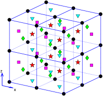
(a) Staggered grid

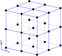
(b) $\mathcal{T}_{h}$

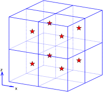
(c) $\mathcal{T}_{h}^{0}$

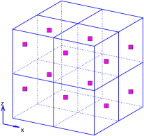
(d) $\mathcal{T}_{h}^{1}$

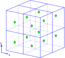
(e) $\mathcal{T}_{h}^{2}$

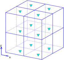
(f) $\mathcal{T}_{h}^{3}$

Figure 1: Illustration of five different grid sets.

A grid point $(x_{l},y_{m},z_{n})\in\mathcal{T}_{h}^{I},I=0,1,2,3,$ is called irregular point if the corresponding finite difference stencils at this point go across the interface $\Gamma$, otherwise it is called regular point. Here $l,m$ and $n$ may take values $i,i-\frac{1}{2},j,j-\frac{1}{2}$ and $k,k-\frac{1}{2}$.

For a function $v(x,y,z)$, set the differential operators

$$\begin{split}\delta_{h,1}^{+}v_{l,m,n}=h^{-1}(v_{l+1,m,n}-v_{l,m,n}),\quad\quad\delta_{h,1}^{-}v_{l,m,n}=h^{-1}(v_{l,m,n}-v_{l-1,m,n}),\\[4.0pt] \delta_{h,2}^{+}v_{l,m,n}=h^{-1}(v_{l,m+1,n}-v_{l,m,n}),\quad\quad\delta_{h,2}^{-}v_{l,m,n}=h^{-1}(v_{l,m,n}-v_{l,m-1,n}),\\[4.0pt] \delta_{h,3}^{+}v_{l,m,n}=h^{-1}(v_{l,m,n+1}-v_{l,m,n}),\quad\quad\delta_{h,3}^{-}v_{l,m,n}=h^{-1}(v_{l,m,n}-v_{l,m,n-1}),\end{split}$$

and the discrete Laplacian operator

$$\begin{split}\Delta_{h}v_{l,m,n}=\delta_{h,1}^{+}\delta_{h,1}^{-}v_{l,m,n}+\delta_{h,2}^{+}\delta_{h,2}^{-}v_{l,m,n}+\delta_{h,3}^{+}\delta_{h,3}^{-}v_{l,m,n},\end{split}$$

where $v_{l,m,n}$ represents $v(x_{l},y_{m},z_{n})$.

Denote the exact solution of interface problem $\eqref{InterfaceUnfied}$ by

$$({\bf u},p)= \Big{(}u^{(1)}(x_{i},y_{j-\frac{1}{2}},z_{k-\frac{1}{2}}),u^{(2)}(x_{i-\frac{1}{2}},y_{j},z_{k-\frac{1}{2}}),u^{(3)}(x_{i-\frac{1}{2}},y_{j-\frac{1}{2}},z_{k}),$$

$$p(x_{i-\frac{1}{2}},y_{j-\frac{1}{2}},z_{k-\frac{1}{2}})\Big{)},$$

and its finite difference approximation by

$$({\bf u}_{h},p_{h})=\big{(}u^{(1)}_{i,j-\frac{1}{2},k-\frac{1}{2}},u^{(2)}_{i-\frac{1}{2},j,k-\frac{1}{2}},u^{(3)}_{i-\frac{1}{2},j-\frac{1}{2},k},p_{i-\frac{1}{2},j-\frac{1}{2},k-\frac{1}{2}}\big{)}.$$

For simplicity of description, denote $I^{(1)},\,I^{(2)},\,I^{(3)},I^{(4)}$ as collections of indices for computational gird nodes, which are given by

$$\begin{split}I^{(1)}&=\{(i,j,k)|\,i=0,1,...,N-1,\;j=1,2,...,N,\;k=1,2,...,N\},\\[2.0pt] I^{(2)}&=\{(i,j,k)|\,i=1,2,...,N,\;j=0,1,...,N-1,\;k=1,2,...,N\},\\[2.0pt] I^{(3)}&=\{(i,j,k)|\,i=1,2,...,N,\;j=1,2,...,N,\;k=0,1,...,N-1\},\\[2.0pt] I^{(4)}&=\{(i,j,k)|\,i=1,2,...,N,\;j=1,2,...,N,\;k=1,2,...,N\}.\end{split}$$

The discretization of the Stokes equations by second-order MAC scheme at a regular grid point reads as:

$$\begin{split}-\mu\Delta_{h}u^{(1)}_{i,j-\frac{1}{2},k-\frac{1}{2}}+\delta^{+}_{h,1}\,p_{i-\frac{1}{2},j-\frac{1}{2},k-\frac{1}{2}}=\tilde{f}^{(1)}_{i,j-\frac{1}{2},k-\frac{1}{2}},\quad\;\;(i,j,k)\in I^{(1)},\\[4.0pt] -\mu\Delta_{h}u^{(2)}_{i-\frac{1}{2},j,k-\frac{1}{2}}+\delta^{+}_{h,2}\,p_{i-\frac{1}{2},j-\frac{1}{2},k-\frac{1}{2}}=\tilde{f}^{(2)}_{i-\frac{1}{2},j,k-\frac{1}{2}},\quad\;\;(i,j,k)\in I^{(2)},\\[4.0pt] -\mu\Delta_{h}u^{(3)}_{i-\frac{1}{2},j-\frac{1}{2},k}+\delta^{+}_{h,3}\,p_{i-\frac{1}{2},j-\frac{1}{2},k-\frac{1}{2}}=\tilde{f}^{(3)}_{i-\frac{1}{2},j-\frac{1}{2},k},\quad\;\;(i,j,k)\in I^{(3)},\\[4.0pt] \delta^{-}_{h,1}u^{(1)}_{i,j-\frac{1}{2},k-\frac{1}{2}}+\delta^{-}_{h,2}u^{(2)}_{i-\frac{1}{2},j,k-\frac{1}{2}}+\delta^{-}_{h,3}u^{(3)}_{i-\frac{1}{2},j-\frac{1}{2},k}=0,\quad\;\;(i,j,k)\in I^{(4)}.\end{split}$$

However, the above MAC scheme has large local truncation errors at an irregular point due to the existence of the interface $\Gamma$. To raise the global accuracy to second order, appropriate correction terms should be added to the right-hand side of the system, so that the coefficient matrix will not be changed. The modified MAC scheme is in the form

$$\begin{split}-\mu\Delta_{h}u^{(1)}_{i,j-\frac{1}{2},k-\frac{1}{2}}+\delta^{+}_{h,1}\,p_{i-\frac{1}{2},j-\frac{1}{2},k-\frac{1}{2}}=f^{(1)}_{i,j-\frac{1}{2},k-\frac{1}{2}},\quad\;\;(i,j,k)\in I^{(1)},\\[4.0pt] -\mu\Delta_{h}u^{(2)}_{i-\frac{1}{2},j,k-\frac{1}{2}}+\delta^{+}_{h,2}\,p_{i-\frac{1}{2},j-\frac{1}{2},k-\frac{1}{2}}=f^{(2)}_{i-\frac{1}{2},j,k-\frac{1}{2}},\quad\;\;(i,j,k)\in I^{(2)},\\[4.0pt] -\mu\Delta_{h}u^{(3)}_{i-\frac{1}{2},j-\frac{1}{2},k}+\delta^{+}_{h,3}\,p_{i-\frac{1}{2},j-\frac{1}{2},k-\frac{1}{2}}=f^{(3)}_{i-\frac{1}{2},j-\frac{1}{2},k},\quad\;\;(i,j,k)\in I^{(3)},\\[4.0pt] \delta^{-}_{h,1}u^{(1)}_{i,j-\frac{1}{2},k-\frac{1}{2}}+\delta^{-}_{h,2}u^{(2)}_{i-\frac{1}{2},j,k-\frac{1}{2}}+\delta^{-}_{h,3}u^{(3)}_{i-\frac{1}{2},j-\frac{1}{2},k}=g_{i-\frac{1}{2},j-\frac{1}{2},k-\frac{1}{2}}\quad\;\;(i,j,k)\in I^{(4)},\end{split}$$ (21)

with

$$\begin{split}&f^{(1)}_{i,j-\frac{1}{2},k-\frac{1}{2}}=\tilde{f}^{(1)}_{i,j-\frac{1}{2},k-\frac{1}{2}}+C\{\mu\Delta u^{(1)}\}_{i,j-\frac{1}{2},k-\frac{1}{2}}+C\{p_{x}\}_{i,j-\frac{1}{2},k-\frac{1}{2}},\\[4.0pt] &f^{(2)}_{i-\frac{1}{2},j,k-\frac{1}{2}}=\tilde{f}^{(2)}_{i-\frac{1}{2},j,k-\frac{1}{2}}+C\{\mu\Delta u^{(2)}\}_{i-\frac{1}{2},j,k-\frac{1}{2}}+C\{p_{y}\}_{i-\frac{1}{2},j,k-\frac{1}{2}},\\[4.0pt] &f^{(3)}_{i-\frac{1}{2},j-\frac{1}{2},k}=\tilde{f}^{(3)}_{i-\frac{1}{2},j-\frac{1}{2},k}+C\{\mu\Delta u^{(3)}\}_{i-\frac{1}{2},j-\frac{1}{2},k}+C\{p_{z}\}_{i-\frac{1}{2},j-\frac{1}{2},k},\\[4.0pt] &g_{i-\frac{1}{2},j-\frac{1}{2},k-\frac{1}{2}}=C\{u^{(1)}_{x}\}_{i-\frac{1}{2},j-\frac{1}{2},k-\frac{1}{2}}+C\{u^{(2)}_{y}\}_{i-\frac{1}{2},j-\frac{1}{2},k-\frac{1}{2}}+C\{u^{(3)}_{z}\}_{i-\frac{1}{2},j-\frac{1}{2},k-\frac{1}{2}}.\end{split}$$

It is noted that the correction terms are the sum of a few leading order terms of Taylor expansions and are non-zero only at irregular points. And they will improve the local truncation errors near the interface to at least first-order accuracy. As one will see in the coming section, these correction terms can be computed in terms of the jumps of the solution and their partial derivatives. As a matter of fact, all jump conditions are also computable by taking the derivatives of the interface conditions together with the incompressible condition.

Let $\boldsymbol{\Delta}_{h}={\rm diag}(\Delta_{h},\Delta_{h},\Delta_{h})$ denote the standard central difference operator, and $G_{h}^{\rm MAC}=(\delta^{+}_{h,1},\delta^{+}_{h,2},\delta^{+}_{h,3})^{T},$ $D_{h}^{\rm MAC}=(\delta^{-}_{h,1},\delta^{-}_{h,2},\delta^{-}_{h,3})$ be the MAC gradient or divergence operator, then the MAC scheme can be rewritten as a linear system in the form of

$$\begin{pmatrix}-\mu\boldsymbol{\Delta}_{h}&G_{h}^{\rm MAC}\\[4.0pt] D_{h}^{\rm MAC}&{\bf 0}\\ \end{pmatrix}\begin{pmatrix}{\bf u}_{h}\\[4.0pt] p_{h}\\ \end{pmatrix}=\begin{pmatrix}{\bf f}\;\\[4.0pt] g\\ \end{pmatrix}.$$ (22)

It is known that the resulting system is a saddle point problem, which must be solved using an iterative method, typically a Krylov subspace method such as GMRES [31]. A wide variety of preconditioners have been proposed for such systems, mainly including domain decomposition methods [25, 8], block preconditioners [10, 13, 5] and multigrid methods [36, 11, 37]. Here, a conjugate gradient (CG) method together with an FFT-based Poisson solver introduced in our previous work [9] has been extended to the present three-dimensional case, which can be included as

• Since the trouble is the uniqueness of the pressure $p_{h}$, an auxiliary variable $\lambda_{h}$ and a parameter $\alpha$ satisfying the condition that $\lambda_{h}$ equals the average of the pressure variable over the domain are introduced to ensure the solvability of the system. Then the linear system reads as

  $$\begin{pmatrix}-\mu\boldsymbol{\Delta}_{h}&G_{h}^{\rm MAC}&0\\[4.0pt] D_{h}^{\rm MAC}&0&-\gamma\\[4.0pt] 0&-\gamma^{T}&\alpha\end{pmatrix}\begin{pmatrix}{\bf u}_{h}\\[4.0pt] p_{h}\\[4.0pt] \lambda_{h}\end{pmatrix}=\begin{pmatrix}{\bf f}\\[4.0pt] g\\[4.0pt] 0\end{pmatrix}.$$ (23)

• Substituting ${\bf u}_{h}=(-\Delta_{h}^{-1}{\bf f}+\Delta_{h}^{-1}G_{h}^{\rm MAC}p_{h})/\mu$ into (23) yields the system

  $$(\frac{1}{\mu}D_{h}^{\rm MAC}\boldsymbol{\Delta}_{h}^{-1}G_{h}^{\rm MAC}+\dfrac{1}{\alpha}\gamma\gamma^{T})p_{h}=\frac{1}{\mu}D_{h}^{\rm MAC}\Delta_{h}^{-1}{\bf f}+g,$$

  which can be solved efficiently by the CG method. Besides, the evaluation of $\Delta_{h}^{-1}$ can be transformed into solving a Poisson equation. Hence an FFT-based Poisson fast solver can be used in each iteration.

• Furthermore, using $p_{h}$ computed from the above system, the velocity ${\bf u}_{h}$ can be solved from

  $$-\mu{\bf\Delta}_{h}{\bf u}_{h}={\bf f}-G_{h}^{\rm MAC}p_{h},$$

  with the FFT-based Poisson solvers again.

It is remarked that no preconditioner for the iterative method is involved in the present method. Efficient algorithms incorporated with preconditioner for the time-dependent problems are encouraging and will be reported in future work.

4.3 Correction of the MAC Scheme

Once again, the discontinuity of the velocity and its stress tensor across the interface $\Gamma$ leads to the fact that the local truncation errors of the finite difference MAC scheme (21) at irregular grid nodes are too large, and the solution to the discrete Stokes interface problem will be inaccurate without any modification. To obtain the desired second-order accuracy, some correction terms have been added to the right hand of the discrete system (21). This subsection presents the detailed derivation of the correction terms. Here, the correction technique is similar to that presented in [46] except that the used grid is staggered grid and the pressure term $p$ is also needed to be modified. For simplicity, only the right side of the x-axis is illustrated, and the correction terms at the opposite sides can be obtained by symmetry. Moreover, the correction terms at the y- or z-direction can be obtained using the same method. Assuming that there is an irregular point on the gird cell in Fig.2 (a), the correction terms are evaluated as follows:

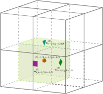
(a) Reference Cell

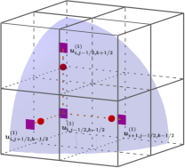
(b) $(x_{i},y_{j-\frac{1}{2}},z_{k-\frac{1}{2}})$

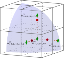
(c) $(x_{i-\frac{1}{2}},y_{j},z_{k-\frac{1}{2}})$

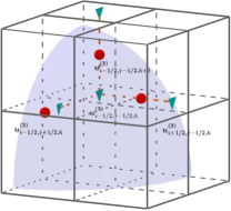
(d) $(x_{i-\frac{1}{2}},y_{j-\frac{1}{2}},z_{k})$

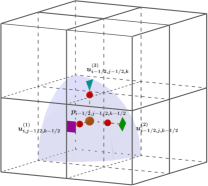
(e) $(x_{i-\frac{1}{2}},y_{j-\frac{1}{2}},z_{k-\frac{1}{2}})$

Figure 2: Illustration of Irregular points.

1. Assume that $(x_{i},y_{j-\frac{1}{2}},z_{k-\frac{1}{2}})$ is an irregular point, see Fig.$\ref{fig-irregular}(b)$ for illustration. In the $x$-direction, denote by $\xi_{u^{(1)}}=x_{i+1}-r$. If $\Gamma$ intersects the grid line segment consisting of point $(x_{i},y_{j-\frac{1}{2}},z_{k-\frac{1}{2}})$ and $(x_{i+1},y_{j-\frac{1}{2}},z_{k-\frac{1}{2}})$ at $(r,y_{j-\frac{1}{2}},z_{k-\frac{1}{2}})$ with $x_{i}<r<x_{i+1}$, the correction term can be computed from Taylor expansion as

$$C\{\mu\Delta u^{(1)}\}_{i,j-\frac{1}{2},k-\frac{1}{2}}=\dfrac{\mu}{h^{2}}\Big{(}[\![u^{(1)}]\!]+\xi_{u^{(1)}}[\![u^{(1)}_{x}]\!]+\dfrac{1}{2}\xi_{u^{(1)}}^{2}[\![u^{(1)}_{xx}]\!]\Big{)},\ \ \hbox{if}\;(x_{i},y_{j-\frac{1}{2}},z_{k-\frac{1}{2}})\in\Omega.$$

2. Assume that $(x_{i-\frac{1}{2}},y_{j},z_{k-\frac{1}{2}})$ is an irregular point, see Fig.$\ref{fig-irregular}(c)$ for illustration. In the $x$-direction, denote by $\xi_{u^{(2)}}=x_{i+\frac{1}{2}}-r$. If $\Gamma$ intersects the grid line segment consisting of point $(x_{i-\frac{1}{2}},y_{j},z_{k-\frac{1}{2}})$ and $(x_{i+\frac{1}{2}},y_{j},z_{k-\frac{1}{2}})$ at $(r,y_{j},z_{k-\frac{1}{2}})$ with $x_{i-\frac{1}{2}}<r<x_{i+\frac{1}{2}}$, the correction term can be computed from Taylor expansion as

$$C\{\mu\Delta u^{(2)}\}_{i-\frac{1}{2},j,k-\frac{1}{2}}=\dfrac{\mu}{h^{2}}\Big{(}[\![u^{(2)}]\!]+\xi_{u^{(2)}}[\![u^{(2)}_{x}]\!]+\dfrac{1}{2}\xi_{u^{(2)}}^{2}[\![u^{(2)}_{xx}]\!]\Big{)},\ \ \hbox{if}\;(x_{i-\frac{1}{2}},y_{j},z_{k-\frac{1}{2}})\in\Omega.$$

3. Assume that $(x_{i-\frac{1}{2}},y_{j-\frac{1}{2}},z_{k})$ is an irregular point, see Fig. $\ref{fig-irregular}(d)$ for illustration. In the $x$-direction, denote by $\xi_{u^{(3)}}=x_{i+\frac{1}{2}}-r$. $\Gamma$ intersects the grid line segment consisting of point $(x_{i-\frac{1}{2}},y_{j-\frac{1}{2}},z_{k})$ and $(x_{i+\frac{1}{2}},y_{j-\frac{1}{2}},z_{k})$ at $(r,y_{j-\frac{1}{2}},z_{k})$ with $x_{i-\frac{1}{2}}<r<x_{i+\frac{1}{2}}$, the correction term can be computed from Taylor expansion as

$$C\{\mu\Delta u^{(3)}\}_{i-\frac{1}{2},j-\frac{1}{2},k}=\dfrac{\mu}{h^{2}}\Big{(}[\![u^{(3)}]\!]+\xi_{u^{(3)}}[\![u^{(3)}_{x}]\!]+\dfrac{1}{2}\xi_{u^{(3)}}^{2}[\![u^{(3)}_{xx}]\!]\Big{)},\ \ \hbox{if}\;(x_{i-\frac{1}{2}},y_{j-\frac{1}{2}},z_{k})\in\Omega.$$

4. Assume that $(x_{i-\frac{1}{2}},y_{j-\frac{1}{2}},z_{k-\frac{1}{2}})$ is an irregular point, see Fig.$\ref{fig-irregular}(e)$ for illustration. In the $x$-direction, denote by $\xi_{u^{(1)}}=x_{i}-r$ and $\xi_{p}=x_{i-\frac{1}{2}}-r$. If $\Gamma$ intersects the grid line segment consisting of point $(x_{i-\frac{1}{2}},y_{j-\frac{1}{2}},z_{k-\frac{1}{2}})$ and $(x_{i},y_{j-\frac{1}{2}},z_{k-\frac{1}{2}})$ at $(r,y_{j-\frac{1}{2}},z_{k-\frac{1}{2}})$ with $x_{i-\frac{1}{2}}<r<x_{i}$, the correction term can be computed from Taylor expansion as

$$C\{u^{(1)}_{x}\}_{i-\frac{1}{2},j-\frac{1}{2},k-\frac{1}{2}}=\dfrac{1}{h}\Big{(}[\![u^{(1)}]\!]+\xi_{u^{(1)}}[\![u^{(1)}_{x}]\!] +\dfrac{1}{2}\xi_{u^{(1)}}^{2}[\![u^{(1)}_{xx}]\!]\Big{)},$$

$$\hbox{if}\;(x_{i-\frac{1}{2}},y_{j-\frac{1}{2}},z_{k-\frac{1}{2}})\in\Omega,$$

and

$$C\{p_{x}\}_{i,j-\frac{1}{2},k-\frac{1}{2}}=\dfrac{1}{h}\Big{(}[\![p]\!]+\xi_{p}[\![p_{x}]\!]\Big{)},\quad\hbox{if}\;(x_{i},y_{j-\frac{1}{2}},z_{k-\frac{1}{2}})\in\Omega.$$

Once the jumps across the interface are computed, the correction terms can be derived explicitly, so that they can be added to the right hand of the discrete linear system (21) at the irregular grid nodes. Thus, the coefficient matrix of the modified system is the same as the standard Stokes problem without an interface and the existing fast solver is still applicable. Besides, the derivation of the correction terms indicates that they improved the local truncation errors near the interface to at least first order accuracy, which is sufficient to recover the formal second-order accuracy of the underlying numerical scheme. Numerical results in section 5 illustrate this fact, and one can refer [9] for the detailed analysis.

In addition, the jump conditions involved in the correction terms can be calculated from the original equations (18a)-(18d), and the details will not be presented here because of the size limitation.

4.4 Interpolation for Integrals on the Interface

It is seen that the approximation solution to the interface problem (18) is calculated on a staggered grid node, while the approximations of the corresponding boundary or volume integral needed in (9) should be evaluated at discretization points of the interface $\Gamma$. To this end, with $({\bf u}_{h},p_{h})$ computed by the MAC scheme (21), a quadratic polynomial interpolation should be designed to extract limit values of ${\bf u}_{h}$ and its flux $\boldsymbol{\sigma}({\bf u},p)$ at any given discretization points ${\bf x}$ on the interface. For a control point ${\bf x}$ on the interface, ten closest grid nodes ${\bf z}_{i}(i=0,1,2,...,9)$ are chosen to construct the interpolation stencil (see Fig. 3 for illustration).

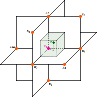
Figure 3: Point ${\bf x}$ on the interface located at one quadrant distribution and the corresponding ten interpolation grid nodes ${\bf z}_{i}$ (nine of them are marked with circle and the other one ${{\bf z}}_{4}$ is hidden behind) for computing the limits values of an approximation solution and its traction.

For each interpolation point ${\bf z}_{i}\in\Omega(i=1,2,...,10)$, Taylor expansion around the point ${\bf x}\in\Gamma$ is given by

$$\begin{split}{\bf u}_{h}({\bf z}_{i})=&{\bf u}_{h}^{+}({\bf x})+\xi_{i}{\bf u}_{h,x}^{+}({\bf x})+\eta_{i}{\bf u}_{h,y}^{+}({\bf x})+\gamma_{i}{\bf u}_{h,z}^{+}({\bf x})\\[4.0pt] &+\frac{1}{2}\xi_{i}^{2}{\bf u}_{h,xx}^{+}({\bf x})+\frac{1}{2}\eta_{i}^{2}{\bf u}_{h,yy}^{+}({\bf x})+\frac{1}{2}\gamma_{i}^{2}{\bf u}_{h,zz}^{+}({\bf x})\\[4.0pt] &+\eta_{i}\gamma_{i}{\bf u}_{h,yz}^{+}({\bf x})+\xi_{i}\gamma_{i}{\bf u}_{h,xz}^{+}({\bf x})+\xi_{i}\eta_{i}{\bf u}_{h,xy}^{+}({\bf x})+O(|{\bf z}_{i}-{\bf x}|^{3}),\end{split}$$ (24)

where ${\bf z}_{i}-{\bf x}\equiv(\xi_{i},\eta_{i},\gamma_{i})^{T}$, ${\bf u}_{h,x}$, ${\bf u}_{h,y}$, ${\bf u}_{h,z}$ are respectively used to denote $\partial{\bf u}_{h}/\partial x$, $\partial{\bf u}_{h}/\partial y$ and $\partial{\bf u}_{h}/\partial z$ and the second order derivatives are defined in a similar way. It is noted that ${\bf z}_{i}$ belongs to different grid sets $\mathcal{T}_{h}^{j}(j=1,2,3)$ for different components $u^{(j)}$. While for each interpolation point ${\bf z}_{i}\in\Omega^{c}$, Taylor expansion around ${\bf x}$ is given by

$$\begin{split}{\bf u}_{h}({\bf z}_{i})=&{\bf u}_{h}^{-}({\bf x})+\xi_{i}{\bf u}_{h,x}^{-}({\bf x})+\eta_{i}{\bf u}_{h,y}^{-}({\bf x})+\gamma_{i}{\bf u}_{h,z}^{-}({\bf x})\\[4.0pt] &+\frac{1}{2}\xi_{i}^{2}{\bf u}_{h,xx}^{-}({\bf x})+\frac{1}{2}\eta_{i}^{2}{\bf u}_{h,yy}^{-}({\bf x})+\frac{1}{2}\gamma_{i}^{2}{\bf u}_{h,zz}^{-}({\bf x})\\[4.0pt] &+\eta_{i}\gamma_{i}{\bf u}_{h,yz}^{-}({\bf x})+\xi_{i}\gamma_{i}{\bf u}_{h,xz}^{-}({\bf x})+\xi_{i}\eta_{i}{\bf u}_{h,xy}^{-}({\bf x})+O(|{\bf z}_{i}-{\bf x}|^{3}),\end{split}$$ (25)

For conciseness, denote the approximate value ${\bf u}_{h}$ and its derivatives respectively by

$$\begin{split}&{\bf v}^{\pm}={\bf u}^{\pm}_{h}({\bf x}),\ \ \ \qquad{\bf v}_{x}^{\pm}={\bf u}^{\pm}_{h,x}({\bf x}),\ \ \qquad{\bf v}_{y}^{\pm}={\bf u}^{\pm}_{h,y}({\bf x}),\\[4.0pt] &{\bf v}_{xx}^{\pm}={\bf u}^{\pm}_{h,xx}({\bf x}),\qquad{\bf v}_{yy}^{\pm}={\bf u}^{\pm}_{h,yy}({\bf x}),\qquad{\bf v}_{zz}^{\pm}={\bf u}^{\pm}_{h,zz}({\bf x}),\\[4.0pt] &{\bf v}_{yz}^{\pm}={\bf u}^{\pm}_{h,yz}({\bf x}),\qquad{\bf v}_{xz}^{\pm}={\bf u}^{\pm}_{h,xz}({\bf x}),\qquad{\bf v}_{xy}^{\pm}={\bf u}^{\pm}_{h,xy}({\bf x}).\end{split}$$

Due to the discontinuity of ${\bf v}({\bf x})$ and its traction across the interface $\Gamma$, the following jump function should be introduced

$$\begin{split}{\bf J}_{i}=&[\![{\bf v}]\!]+\xi_{i}[\![{\bf v}_{x}]\!]+\eta_{i}[\![{\bf v}_{y}]\!]+\gamma_{i}[\![{\bf v}_{z}]\!]+\frac{1}{2}\xi_{i}^{2}[\![{\bf v}_{xx}]\!]+\frac{1}{2}\eta_{i}^{2}[\![{\bf v}_{yy}]\!]+\frac{1}{2}\gamma_{i}^{2}[\![{\bf v}_{zz}]\!]\\[4.0pt] &+\eta_{i}\gamma_{i}[\![{\bf v}_{yz}]\!]+\xi_{i}\gamma_{i}[\![{\bf v}_{xz}]\!]+\xi_{i}\eta_{i}[\![{\bf v}_{xy}]\!].\end{split}$$

Thus, Taylor expansion (24) and (25) can be rewritten as

$$\begin{split}\;\qquad{\bf v}_{i}=&{\bf v}^{+}+\xi_{i}{\bf v}_{x}^{+}+\eta_{i}{\bf v}_{y}^{+}+\gamma_{i}{\bf v}_{z}^{+}+\frac{1}{2}\xi_{i}^{2}{\bf v}_{xx}^{+}+\frac{1}{2}\eta_{i}^{2}{\bf v}_{yy}^{+}+\frac{1}{2}\gamma_{i}^{2}{\bf v}_{zz}^{+}\\[4.0pt] &+\eta_{i}\gamma_{i}{\bf v}_{yz}^{+}+\xi_{i}\gamma_{i}{\bf v}_{xz}^{+}+\xi_{i}\eta_{i}{\bf v}_{xy}^{+},\quad{\rm if}\ {\bf z}_{i}\in\Omega,\end{split}$$

and

$$\begin{split}{\bf v}_{i}+{\bf J}_{i}=&{\bf v}^{+}+\xi_{i}{\bf v}_{x}^{+}+\eta_{i}{\bf v}_{y}^{+}+\gamma_{i}{\bf v}_{z}^{+}+\frac{1}{2}\xi_{i}^{2}{\bf v}_{xx}^{+}+\frac{1}{2}\eta_{i}^{2}{\bf v}_{yy}^{+}+\frac{1}{2}\gamma_{i}^{2}{\bf v}_{zz}^{+}\\[4.0pt] &+\eta_{i}\gamma_{i}{\bf v}_{yz}^{+}+\xi_{i}\gamma_{i}{\bf v}_{xz}^{+}+\xi_{i}\eta_{i}{\bf v}_{xy}^{+},\quad{\rm if}\ {\bf z}_{i}\in\Omega^{c}.\end{split}$$

Here, the third-order term $O(|{\bf z}_{i}-{\bf x}|^{3})$ is omitted.

Solving the linear system above, one could obtain the limit value of ${\bf u}_{h}$ on the interface $\Gamma$. Since the stress tensor $\boldsymbol{\sigma}({\bf u}_{h},p_{h})$ does not involve the derivatives of $p_{h}$, linear interpolation is enough in the evaluation of boundary value $p_{h}$, which can be done similarly and will be omitted here.

5 Numerical Results

Numerical tests are designed in this section to investigate the accuracy, efficiency and robustness of the proposed method for solving 3D Stokes and Navier boundary value problems. To this end, the normalized maximum norms and $\ell^{2}$-norms are defined as follows

$$\|e_{p}\|_{\infty}=\frac{\|p-p_{h}\|_{\infty}}{\|p\|_{\infty}},\qquad\qquad\|e_{u^{(i)}}\|_{\infty}=\frac{\|u^{(i)}-u_{h}^{(i)}\|_{\infty}}{\|u^{(i)}\|_{\infty}},\quad\quad i=1,2,3,$$

and

$$\|e_{p}\|_{2}=\frac{\|p-p_{h}\|_{2}}{\|p\|_{2}},\qquad\qquad\|e_{u^{(i)}}\|_{2}=\frac{\|u^{(i)}-u_{h}^{(i)}\|_{2}}{\|u^{(i)}\|_{2}},\qquad\;\quad i=1,2,3.$$

In all the examples, the GMRES iterative method is employed to solve the discrete boundary integral equations. The GMRES iteration starts with a zero initial guess and stops when the iterated residual in the discrete $\ell^{2}$-norm relative to that of the initial residual is less than a prescribed tolerance $\epsilon=10^{-9}$. Furthermore, the corresponding bounding cube for the interface problem is set to $\mathcal{B}=[-1.2,1.2]^{3}$.

5.1 Examples for Stokes problems

Three Stokes problems on different 3D irregular domains are considered in this subsection. Numerical results are listed in Tables 1-6. The grid sizes are listed in the first column, and the number of GMRES iterations is recorded in the second column. The third to the last columns show the errors of the numerical solution in discrete maximum and $\ell^{2}$-norm, as well as the convergence rates. The color mapped numerical solution ${\bf u}_{h}$ and $p_{h}$ on a $256\times 256$ mesh are shown in Fig. 4-6. It is noted that a fine mesh is used in all plots presented in this section for a better resolution of the irregular boundary.

Example 5.1. This example solves the Stokes Dirichlet problem on a sphere with radius $r=1$, which is located at the origin of the coordinates. The exact solution is given by

$$\begin{cases}u^{(1)}=x^{2}(2-x^{2})+4xy(x^{2}+y^{2}-1)+z^{2}(3z^{2}-6x^{2}-2),\\[4.0pt] u^{(2)}=x^{2}(3x^{2}-6y^{2}-1)+y^{2}(1-y^{2}),\\[4.0pt] u^{(3)}=4zx(z^{2}+x^{2}-1),\\[4.0pt] \;\quad p=8y(3x^{2}-y^{2})+8x(3z^{2}-x^{2}).\end{cases}$$

The external forcing term ${\bf f}$ and the boundary condition ${\bf g}$ can be determined from the exact solution. The errors and convergence rates in the maximum norms and $\ell^{2}$ norms are shown in Table 1 and Table 2 respectively, which indicate that the velocity is of second-order accuracy in both the discrete maximum and $\ell^{2}$ norm, and the pressure is also second-order accurate in the $\ell^{2}$ norm. The numbers of GMRES iterations are also presented, which shows that the number of GMRES iterations is independent of the size of the mesh.

Table 1: Maximum error and convergence rates of Example 1

N	# step	$\|e_{{\bf u}_{1}}\|_{\infty}$	rate	$\|e_{{\bf u}_{2}}\|_{\infty}$	rate	$\|e_{{\bf u}_{3}}\|_{\infty}$	rate	$\|e_{p}\|_{\infty}$	rate
64	12	4.80e-3	-	3.65e-3	-	9.23e-3	-	2.33e-2	-
128	11	5.59e-4	3.10	6.84e-4	2.42	1.39e-3	2.73	6.40e-3	1.86
256	11	9.55e-5	2.55	8.67e-5	2.98	1.31e-4	3.41	1.91e-3	1.74
512	11	1.34e-5	2.83	1.44e-5	2.59	1.78e-5	2.88	6.06e-4	1.66

Table 2: $\ell^{2}$-error and convergence rates of Example 1

grid size	$\|e_{{\bf u}_{1}}\|_{2}$	rate	$\|e_{{\bf u}_{2}}\|_{2}$	rate	$\|e_{{\bf u}_{3}}\|_{2}$	rate	$\|e_{p}\|_{2}$	rate
64	1.06e-3	-	9.16e-4	-	1.40e-3	-	5.46e-3	-
128	9.12e-5	3.54	8.73e-5	3.39	1.18e-4	3.57	9.56e-4	2.51
256	1.12e-5	3.03	9.72e-6	3.17	1.57e-5	2.91	2.04e-4	2.23
512	1.43e-6	2.97	1.37e-6	2.83	1.92e-6	3.03	3.82e-5	2.42

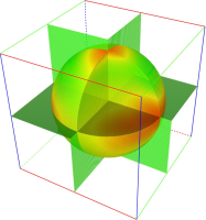
(a) $u_{h}^{(1)}$

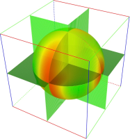
(b) $u_{h}^{(2)}$

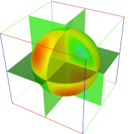
(c) $u_{h}^{(3)}$

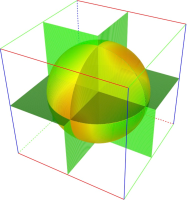
(d) $p_{h}$

Figure 4: Numerical solution ${\bf u}_{h}$ and $p_{h}$ in a sphere for Stokes problem.

Example 5.2. In this example, the computational domain is an ellipsoid

$$\Big{\{}(x,y,z)\ |\ x^{2}+\dfrac{y^{2}}{0.64}+\dfrac{z^{2}}{0.36}=1.\Big{\}}$$

Consider the exact solution

$$\begin{cases}u^{(1)}=2x^{3}y/3-z^{2}x^{2}+e^{z}+\sin(\pi z),\\[4.0pt] u^{(2)}=-x^{2}y^{2}+\cos(\pi x),\\[4.0pt] u^{(3)}=2z^{3}x/3+e^{x}+\sin(\pi x),\\[4.0pt] \;\quad p=(x-1)^{3}(y-1)^{3}(z-1)^{3}.\end{cases}$$

Normalized errors for the velocity components $u^{(1)}$, $u^{(2)}$, $u^{(3)}$ and the pressure $p$ in the discrete maximum norm and the $\ell^{2}$ norm are listed separately in Table 3 and 4. It can be seen that the components of velocity are all second-order accurate in both the discrete maximum norm and discrete $\ell^{2}$ norm, and the pressure is second accurate in $\ell^{2}$ norm. The GMRES iteration number for different mesh sizes is also shown in Table 3-4.

Table 3: Maximum error and convergence rates of Example 2

N	# step	$\|e_{{\bf u}_{1}}\|_{\infty}$	rate	$\|e_{{\bf u}_{2}}\|_{\infty}$	rate	$\|e_{{\bf u}_{3}}\|_{\infty}$	rate	$\|e_{p}\|_{\infty}$	rate
128	14	5.44e-4	-	7.65e-4	-	2.53e-4	-	2.22e-2	-
256	15	5.94e-5	3.20	8.01e-5	3.26	4.13e-5	2.61	7.05e-3	1.65
512	14	8.44e-6	2.82	2.07e-5	1.95	6.80e-6	2.60	1.77e-3	1.99

Table 4: $\ell^{2}$-error and convergence rates of Example 2

N	$\|e_{{\bf u}_{1}}\|_{2}$	rate	$\|e_{{\bf u}_{2}}\|_{2}$	rate	$\|e_{{\bf u}_{3}}\|_{2}$	rate	$\|e_{p}\|_{2}$	rate
128	2.95e-5	-	6.43e-5	-	1.82e-5	-	1.14e-3	-
256	6.02e-6	2.29	1.26e-5	2.35	4.18e-6	2.12	2.94e-4	1.96
512	1.29e-6	2.22	2.07e-6	2.61	9.42e-7	2.15	9.10e-5	1.69

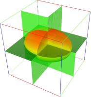
(a) $u_{h}^{(1)}$

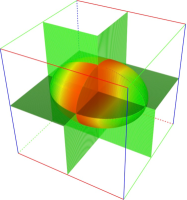
(b) $u_{h}^{(2)}$

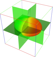
(c) $u_{h}^{(3)}$

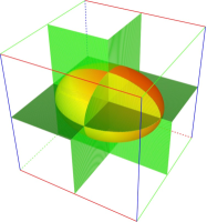
(d) $p_{h}$

Figure 5: Numerical solution ${\bf u}_{h}$ and $p_{h}$ in an ellipsoid for Stokes problem.

Example 5.3. In this example, a more complicated domain is considered, which is given by

$$\Omega=\{(x,y,z)\in\mathcal{R}^{3}:(c-\sqrt{(x^{2}+y^{2})})^{2}+z^{2}<a^{2}\}$$

with $a=0.35$ and $c=0.7$. The exact solution is determined by:

$$\begin{cases}u^{(1)}=-4xy(1-x^{2}-y^{2})-x^{2}(x^{2}+6z^{2}-2)+z^{2}(3z^{2}-2)\\[4.0pt] \quad\quad+\exp(\cos y)+\exp(\sin z),\\[4.0pt] u^{(2)}=x^{2}(3x^{2}-6y^{2}-2)-y^{2}(y^{2}-2)+\exp(\sin x),\\[4.0pt] u^{(3)}=-4(1-x^{2}-z^{2})xz+\exp(\cos x),\\[4.0pt] \quad\;p=\exp(1-y^{2}-z^{3})\sin(x^{2}+1).\end{cases}$$

The maximum errors, $\ell^{2}$-errors and the corresponding convergence rates are displayed in Table 5-6, which indicate that second-order accuracy of the solutions $({\bf u}_{h},p_{h})$ is achieved. And the number of GMRES iterations shown in the second column of the tables is almost independent of the mesh size.

Table 5: Maximum error and convergence rates of Example 3

N	# step	$\|e_{{\bf u}_{1}}\|_{\infty}$	rate	$\|e_{{\bf u}_{2}}\|_{\infty}$	rate	$\|e_{{\bf u}_{3}}\|_{\infty}$	rate	$\|e_{p}\|_{\infty}$	rate
128	24	8.97e-4	-	8.29e-4	-	7.42e-4	-	5.54e-1	-
256	26	7.54e-5	3.57	5.80e-5	3.84	6.19e-5	3.58	1.00e-1	2.47
512	26	1.01e-5	2.90	9.86e-6	2.56	1.32e-5	2.23	1.86e-2	2.43

Table 6: $\ell^{2}$-error and its convergence rates of Example 3

N	$\|e_{{\bf u}_{1}}\|_{2}$	rate	$\|e_{{\bf u}_{2}}\|_{2}$	rate	$\|e_{{\bf u}_{3}}\|_{2}$	rate	$\|e_{p}\|_{2}$	rate
128	2.22e-5	-	7.64e-5	-	2.62e-5	-	1.50e-2	-
256	4.74e-6	2.23	1.26e-5	2.60	3.95e-6	2.73	2.94e-3	2.35
512	1.03e-6	2.20	2.50e-6	2.33	9.14e-7	2.11	8.82e-4	1.74

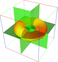
(a) $u_{h}^{(1)}$

(b) $u_{h}^{(2)}$

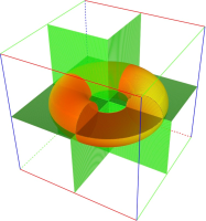
(c) $u_{h}^{(3)}$

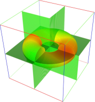
(d) $p_{h}$

Figure 6: Numerical solution ${\bf u}_{h}$ and $p_{h}$ in a torus for Stokes problem.

5.2 Examples for Navier problems

To test the efficiency of the KFBI for the Navier boundary value problems, three examples are considered here. Numerical results are listed in Tables 7-12. Each table has eight columns, showing the size of the Cartesian grid, the numbers of the GMRES iteration in solving BIE, the errors of the numerical solution in the maximum norm or discrete $\ell^{2}$-norm, as well as the convergence rates. Fig. 4-6 show the color mapped numerical solution ${\bf u}_{h}$ of each example on a $256\times 256$ mesh respectively.

Example 5.4. In this example, the computational domain is a sphere, which is given by $x^{2}+y^{2}+z^{2}=1$. The exact solution is determined by:

$$\begin{cases}u^{(1)}=\sin(2\pi r^{2})\cos(2y)\cos(z),\\[3.0pt] u^{(2)}=\sin(2\pi r^{2})\cos(x)\cos(x+z),\\[3.0pt] u^{(3)}=\sin(2\pi r^{2})\cos(\pi x)\cos(y).\end{cases}$$

The material data are chosen as $E=1000$, and $\nu=1/10$. The maximum errors and the corresponding convergence rates are displayed in Table 7. The $\ell^{2}$-errors and the corresponding convergence rates are shown in Table 8. As expected, the proposed method is second-order accurate for the numerical solutions. Additionally, the number of iterations does not depend on the mesh size and it is a relatively small number.

Table 7: Maximum-error and its convergence rates of Example 4.4

N	# step	$\|e_{{\bf u}_{1}}\|_{2}$	rate	$\|e_{{\bf u}_{2}}\|_{2}$	rate	$\|e_{{\bf u}_{3}}\|_{2}$	rate
64	14	1.50e-2	-	1.33e-2	-	1.60e-2	-
128	14	4.09e-3	1.87	3.03e-3	2.13	4.02e-3	1.99
256	14	9.97e-4	2.04	7.98e-4	1.92	9.81e-4	2.03
512	15	2.62e-4	1.92	2.10e-4	1.93	2.60e-4	1.92

Table 8: $\ell^{2}$-error and its convergence rates of Example 4.4

N	$\|e_{{\bf u}_{1}}\|_{2}$	rate	$\|e_{{\bf u}_{2}}\|_{2}$	rate	$\|e_{{\bf u}_{3}}\|_{2}$	rate
64	9.03e-3	-	8.03e-3	-	9.63e-3	-
128	2.12e-3	2.09	1.90e-3	2.08	2.29e-3	2.07
256	4.05e-4	2.39	3.84e-4	2.31	4.97e-4	2.20
512	1.01e-4	2.00	9.65e-5	1.99	1.25e-4	1.99

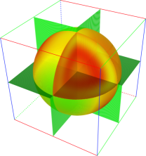
(a) $u_{h}^{(1)}$

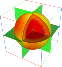
(b) $u_{h}^{(2)}$

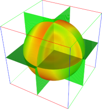
(c) $u^{(3)}_{h}$

Figure 7: Numerical solution ${\bf u}_{h}$ in a sphere for Navier problem.

Example 5.5. This example solves the Navier equations on an ellipsoid domain, which is determined by $x^{2}/r_{a}^{2}+y^{2}/r_{b}^{2}+z^{2}/r_{c}^{2}=1$ with $r_{a}=1,r_{b}=0.8,r_{c}=0.6$. The exact solution is given by

$$\begin{cases}u^{(1)}=x^{2}+y^{2}+z^{2}-4+\cos x\cos y\cos z,\\[4.0pt] u^{(2)}=x^{2}+y^{2}+z^{2}-4+xy+\cos x\cos y\cos z,\\[4.0pt] u^{(3)}=x^{2}+y^{2}+z^{2}-4+yz+\cos x\cos y\cos z.\end{cases}$$

The material data are chosen as $E=4000$, and $\nu=1/20$. Numerical results with second-order accuracy are summarized in Tables 9 and 10. The efficiency and accuracy of the numerical solution observed here are consistent with Example 4.4.

Table 9: Maximum-error and its convergence rates of Example 4.5

N	# step	$\|e_{{\bf u}_{1}}\|_{2}$	rate	$\|e_{{\bf u}_{2}}\|_{2}$	rate	$\|e_{{\bf u}_{3}}\|_{2}$	rate
64	13	1.43e-3	-	1.35e-3	-	2.12e-4	-
128	13	3.44e-4	2.06	2.90e-4	2.22	3.17e-4	2.74
256	13	1.03e-4	1.74	7.66e-5	1.92	8.41e-5	1.91
512	14	2.91e-5	1.82	1.99e-5	1.94	2.15e-5	1.97

Table 10: $\ell^{2}$-error and its convergence rates of Example 4.5

N	$\|e_{{\bf u}_{1}}\|_{2}$	rate	$\|e_{{\bf u}_{2}}\|_{2}$	rate	$\|e_{{\bf u}_{3}}\|_{2}$	rate
64	8.60e-5	-	1.04e-4	-	6.87e-5	-
128	1.96e-5	2.13	1.99e-5	2.39	1.45e-5	2.24
256	4.66e-6	1.95	4.53e-6	2.14	3.73e-6	1.96
512	1.19e-6	1.97	1.15e-6	1.98	9.63e-7	1.95

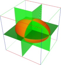
(a) $u_{h}^{(1)}$

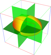
(b) $u_{h}^{(2)}$

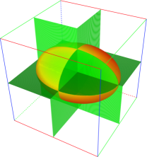
(c) $u^{(3)}_{h}$

Figure 8: Numerical solution ${\bf u}_{h}$ in a ellipsoid for Navier problem.

Example 5.6. This example solves the problem (2a)-(2b) on a torus which is determined by

$$\Omega=\big{\{}(x,y,z)\in R^{3}:(c-\sqrt{x^{2}+y^{2}})^{2}+z^{2}<a^{2}\big{\}}$$

with $a=0.35$ and $c=0.7$. The exact solution is chosen by

$$\begin{cases}u_{1}=\exp(1-y^{2}-z^{2})\sin(3x^{2}+2),\\[1.0pt] u_{2}=\sin(1-x^{2}-y^{2}-z^{2}),\\[1.0pt] u_{3}=3x^{2}+2y^{2}+z^{2}.\end{cases}$$

The material data are chosen as $E=2000$, and $\nu=2/5$. The numerical results in Tables 11 and 12 verify that the GMRES iteration number is essentially independent of the mesh size and the proposed method also yields second-order accurate solutions.

Table 11: Maximum-error and its convergence rates of Example 4.6

N	# step	$\|e_{{\bf u}_{1}}\|_{2}$	rate	$\|e_{{\bf u}_{2}}\|_{2}$	rate	$\|e_{{\bf u}_{3}}\|_{2}$	rate
128	18	9.18e-3	-	8.43e-3	-	3.31e-3	-
256	19	1.90e-3	2.27	1.93e-3	2.13	7.20e-4	2.20
512	19	4.95e-4	1.94	4.99e-4	1.95	1.92e-4	1.91

Table 12: $\ell^{2}$-error and its convergence rates of Example 4.6

N	$\|e_{{\bf u}_{1}}\|_{2}$	rate	$\|e_{{\bf u}_{2}}\|_{2}$	rate	$\|e_{{\bf u}_{3}}\|_{2}$	rate
128	8.74e-4	-	1.08e-3	-	3.30e-4	-
256	1.77e-4	2.30	2.34e-4	2.21	7.22e-5	2.19
512	4.55e-5	1.96	5.94e-5	1.98	1.84e-5	1.97

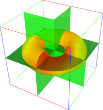
(a) $u_{h}^{(1)}$

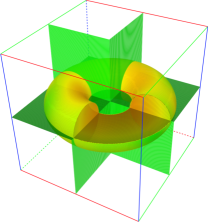
(b) $u_{h}^{(2)}$

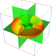
(c) $u_{h}^{(3)}$

Figure 9: Numerical solution ${\bf u}_{h}$ in a torus for Navier problem.

6 Conclusions and Discussions

In this paper, a global second-order KFBI method based on the MAC scheme is proposed to solve the three-dimensional Stokes and Navier boundary value problems on irregular domains. It solves the irregular boundary value problems in the framework of boundary integral equations, but is different from traditional BIM in that the volume or boundary integral is evaluated indirectly. It avoids direct evaluation of nearly singular, singular or hyper-singular boundary integrals, even the requirement of the analytical expressions of Green’s functions.

The reformulated boundary integral equations are Fredholm integral equations of the second kind and can be solved by a Krylov subspace method, such as the GMRES, with the number of iterations being essentially independent of the mesh size. In each GMRES iteration, by posing the Stokes equations in a slightly generalized form that includes a pressure term in the continuity equation, the equivalent simple Stokes and Navier interface problems for integral evaluations can be rewritten into a uniform formulation and then be discretized with a modified MAC scheme. Then the discrete system of this scheme is solved efficiently by the CG method together with an FFT-based Poisson solver. This approach provides a general algorithmic template for solving two- or multi-fluid problems.

In addition, the discretization of the surface plays an important role in the KFBI method. This work uses intersection points of the boundary with the grid lines to represent the surface discretization. The advantage of using intersection points is that it is convenient to find the interpolation stencils, capable to achieve high-order accuracy schemes, and good for problems with moving boundaries.

Nevertheless, the method can be further improved in several aspects. For example, it suffers deterioration in performance in some cases as the Poisson ratio approaches $1/2$ (i.e., as the material becomes incompressible) for the Navier problem. To solve an almost incompressible elastic material, the technique based on an appropriate decomposition of the Kelvin tensor in [33] gives us some ideas. This work only describes the details for a second-order version of the KFBI method in three dimensions. In principle, it is natural and straightforward to derive high-order extensions of this method for fluid and solid mechanics. Furthermore, the application of the KFBI method to Stokes-Darcy problems, and Solid-Fluid interaction will be our future work.

References

- Abousleiman, Y. and Cheng, AH-D [1994] Abousleiman, Y. and Cheng, AH-D, 1994. Boundary element solution for steady and unsteady Stokes flow. Computer Methods in Applied Mechanics and Engineering 117 (1-2), 1–13.
- Beale, J. Thomas [2004] Beale, J. Thomas , 2004. A grid-based boundary integral method for elliptic problems in three dimensions. SIAM Journal on Numerical Analysis 42 (2), 599–620.
- Beale, J Thomas and Lai, Ming-Chih [2001] Beale, J Thomas and Lai, Ming-Chih, 2001. A method for computing nearly singular integrals. SIAM Journal on Numerical Analysis 38 (6), 1902–1925.
- Biros, George and Ying, Lexing and Zorin, Denis [2004] Biros, George and Ying, Lexing and Zorin, Denis, 2004. A fast solver for the Stokes equations with distributed forces in complex geometries. Journal of Computational Physics 193 (1), 317–348.
- Bootland, Niall and Bentley, Alistair and Kees, Christopher and Wathen, Andrew [2019] Bootland, Niall and Bentley, Alistair and Kees, Christopher and Wathen, Andrew, 2019. Preconditioners for two-phase incompressible Navier–Stokes flow. SIAM Journal on Scientific Computing 41 (4), B843–B869.
- Cao, Yue and Xie, Yaning and Krishnamurthy, Mahesh and Li, Shuwang and Ying, Wenjun [2022] Cao, Yue and Xie, Yaning and Krishnamurthy, Mahesh and Li, Shuwang and Ying, Wenjun, 2022. A kernel-free boundary integral method for elliptic PDEs on a doubly connected domain. Journal of Engineering Mathematics 136 (1), 1–21.
- Chessa, Jack and Belytschko, Ted [2003] Chessa, Jack and Belytschko, Ted, 2003. An extended finite element method for two-phase fluids. Journal of Applied Mechanics 70 (1), 10–17.
- Cyr, Eric C and Shadid, John N and Tuminaro, Raymond S [2012] Cyr, Eric C and Shadid, John N and Tuminaro, Raymond S, 2012. Stabilization and scalable block preconditioning for the Navier–Stokes equations. Journal of Computational Physics 231 (2), 345–363.
- Dong, Haixia and Zhao, Zhongshu and Li, Shuwang and Ying, Wenjun And Zhang, jiwei [2023] Dong, Haixia and Zhao, Zhongshu and Li, Shuwang and Ying, Wenjun And Zhang, jiwei, 2023. Second order convergence of a modified MAC scheme for Stokes interface problem. arXiv preprint arXiv:2302.08033.
- Elman, Howard and Howle, Victoria E and Shadid, John and Shuttleworth, Robert and Tuminaro, Ray [2006] Elman, Howard and Howle, Victoria E and Shadid, John and Shuttleworth, Robert and Tuminaro, Ray, 2006. Block preconditioners based on approximate commutators. SIAM Journal on Scientific Computing 27 (5), 1651–1668.
- Elman, Howard C [1996] Elman, Howard C, 1996. Multigrid and krylov subspace methods for the discrete Stokes equations. International Journal for Numerical Methods in Fluids 22 (8), 755–770.
- Greengard, Leslie and Kropinski, Mary Catherine and Mayo, Anita [1996] Greengard, Leslie and Kropinski, Mary Catherine and Mayo, Anita, 1996. Integral equation methods for Stokes flow and isotropic elasticity in the plane. Journal of Computational Physics 125 (2), 403–414.
- Griffith, Boyce E [2009] Griffith, Boyce E, 2009. An accurate and efficient method for the incompressible Navier–Stokes equations using the projection method as a preconditioner. Journal of Computational Physics 228 (20), 7565–7595.
- Grigoriev, MM and Dargush, GF [2005] Grigoriev, MM and Dargush, GF, 2005. A multi-level boundary element method for Stokes flows in irregular two-dimensional domains. Computer Methods in Applied Mechanics and Engineering 194 (34-35), 3553–3581.
- Hansbo, Peter and Larson, Mats G and Zahedi, Sara [2014] Hansbo, Peter and Larson, Mats G and Zahedi, Sara, 2014. A cut finite element method for a Stokes interface problem. Applied Numerical Mathematics 85, 90–114.
- He, Xiaoming and Lin, Tao and Lin, Yanping [2011] He, Xiaoming and Lin, Tao and Lin, Yanping, 2011. Immersed finite element methods for elliptic interface problems with non-homogeneous jump conditions. International Journal of Numerical Analysis & Modeling 8 (2).
- Hsiao, George C and Wendland, Wolfgang L [2008] Hsiao, George C and Wendland, Wolfgang L, 2008. Boundary integral equations. Springer.
- Huang, Q and Cruse, TA1231438 [1993] Huang, Q and Cruse, TA1231438, 1993. Some notes on singular integral techniques in boundary element analysis. International Journal for Numerical Methods in Engineering 36 (15), 2643–2659.
- Jiang, Shidong and Veerapaneni, Shravan and Greengard, Leslie [2012] Jiang, Shidong and Veerapaneni, Shravan and Greengard, Leslie, 2012. Integral equation methods for unsteady Stokes flow in two dimensions. SIAM Journal on Scientific Computing 34 (4), A2197–A2219.
- Jones, Derrick and Zhang, Xu [2021] Jones, Derrick and Zhang, Xu, 2021. A class of nonconforming immersed finite element methods for Stokes interface problems. Journal of Computational and Applied Mathematics 392, 113493.
- Klaseboer, Evert and Sun, Qiang and Chan, Derek YC [2012] Klaseboer, Evert and Sun, Qiang and Chan, Derek YC, 2012. Non-singular boundary integral methods for fluid mechanics applications. Journal of Fluid Mechanics 696, 468–478.
- Kress, Rainer and Maz’ya, V and Kozlov, V [1989] Kress, Rainer and Maz’ya, V and Kozlov, V, 1989. Linear integral equations. Vol. 17. Springer.
- Layton, William J and Schieweck, Friedhelm and Yotov, Ivan [2002] Layton, William J and Schieweck, Friedhelm and Yotov, Ivan, 2002. Coupling fluid flow with porous media flow. SIAM Journal on Numerical Analysis 40 (6), 2195–2218.
- Leveque, Randall J and Li, Zhilin [1994] Leveque, Randall J and Li, Zhilin, 1994. The immersed interface method for elliptic equations with discontinuous coefficients and singular sources. SIAM Journal on Numerical Analysis 31 (4), 1019–1044.
- Lin, Paul T and Sala, Marzio and Shadid, John N and Tuminaro, Ray S [2006] Lin, Paul T and Sala, Marzio and Shadid, John N and Tuminaro, Ray S, 2006. Performance of fully coupled algebraic multilevel domain decomposition preconditioners for incompressible flow and transport. International Journal for Numerical Methods in Engineering 67 (2), 208–225.
- Mayo, Anita [1984] Mayo, Anita, 1984. The fast solution of Poisson’s and the biharmonic equations on irregular regions. SIAM Journal on Numerical Analysis 21 (2), 285–299.
- Mayo, Anita [1985] Mayo, Anita, 1985. Fast high order accurate solution of Laplace’s equation on irregular regions. SIAM Journal on Scientific and Statistical Computing 6 (1), 144–157.
- Mayo, Anita [1992] Mayo, Anita, 1992. The rapid evaluation of volume integrals of potential theory on general regions. Journal of Computational Physics 100 (2), 236–245.
- Peskin, Charles S [1977] Peskin, Charles S, 1977. Numerical analysis of blood flow in the heart. Journal of Computational Physics 25 (3), 220–252.
- Rachh, Manas and Greengard, Leslie [2016] Rachh, Manas and Greengard, Leslie, 2016. Integral equation methods for elastance and mobility problems in two dimensions. SIAM Journal on Numerical Analysis 54 (5), 2889–2909.
- Saad, Youcef and Schultz, Martin H [1986] Saad, Youcef and Schultz, Martin H, 1986. GMRES: A generalized minimal residual algorithm for solving nonsymmetric linear systems. SIAM Journal on Scientific and Statistical Computing 7 (3), 856–869.
- Silva, Goncalo and Ginzburg, Irina [2016] Silva, Goncalo and Ginzburg, Irina, 2016. Stokes–Brinkman–Darcy solutions of bimodal porous flow across periodic array of permeable cylindrical inclusions: cell model, lubrication theory and LBM/FEM numerical simulations. Transport in Porous Media 111 (3), 795–825.
- Steinbach, Olaf [2007] Steinbach, Olaf, 2007. Numerical approximation methods for elliptic boundary value problems: finite and boundary elements. Springer Science & Business Media.
- Tan, Zhijun and Lim, KM and Khoo, BC [2011] Tan, Zhijun and Lim, KM and Khoo, BC, 2011. An implementation of MAC grid-based IIM-Stokes solver for incompressible two-phase flows. Communications in Computational Physics 10 (5), 1333–1362.
- Tlupova, Svetlana and Beale, J Thomas [2013] Tlupova, Svetlana and Beale, J Thomas, 2013. Nearly singular integrals in 3D Stokes flow. Communications in Computational Physics 14 (5), 1207–1227.
- Vanka, S Pratap [1986] Vanka, S Pratap, 1986. Block-implicit multigrid solution of Navier-Stokes equations in primitive variables. Journal of Computational Physics 65 (1), 138–158.
- Wang, Ming and Chen, Long [2013] Wang, Ming and Chen, Long, 2013. Multigrid methods for the stokes equations using distributive Gauss–Seidel relaxations based on the least squares commutator. Journal of Scientific Computing 56, 409–431.
- Wang, Nan and Chen, Jinru [2019] Wang, Nan and Chen, Jinru, 2019. A nonconforming Nitsche’s extended finite element method for Stokes interface problems. Journal of Scientific Computing 81, 342–374.
- Wang, Weiyi and Tan, Zhijun [2021] Wang, Weiyi and Tan, Zhijun, 2021. A simple 3D immersed interface method for Stokes flow with singular forces on staggered grids. Communications in Computational Physics 30 (1), 227–254.
- Wei, Guo-Wei [2010] Wei, Guo-Wei, 2010. Differential geometry based multiscale models. Bulletin of Mathematical Biology 72 (6), 1562–1622.
- Wei, Guo-Wei [2013] Wei, Guo-Wei, 2013. Multiscale, multiphysics and multidomain models I: Basic theory. Journal of Theoretical and Computational Chemistry 12 (08), 1341006.
- Xie, Yaning and Ying, Wenjun [2019] Xie, Yaning and Ying, Wenjun, 2019. A fourth-order kernel-free boundary integral method for the modified Helmholtz equation. Journal of Scientific Computing 78 (3), 1632–1658.
- Xie, Yaning and Ying, Wenjun [2020] Xie, Yaning and Ying, Wenjun, 2020. A high-order kernel-free boundary integral method for incompressible flow equations in two space dimensions. Numerical Mathematics: Theory, Methods & Applications 13 (3).
- Ying, Wenjun [2018] Ying, Wenjun, 2018. A Cartesian grid-based boundary integral method for an elliptic interface problem on closely packed cells. Communications in Computational Physics 24 (4), 1196–1220.
- Ying, Wenjun and Henriquez, Craig S [2007] Ying, Wenjun and Henriquez, Craig S, 2007. A kernel-free boundary integral method for elliptic boundary value problems. Journal of Computational Physics 227 (2), 1046–1074.
- Ying, Wenjun and Wang, Wei-Cheng [2013] Ying, Wenjun and Wang, Wei-Cheng, 2013. A kernel-free boundary integral method for implicitly defined surfaces. Journal of Computational Physics 252, 606–624.
- Ying, Wenjun and Wang, Wei-Cheng [2014] Ying, Wenjun and Wang, Wei-Cheng, 2014. A kernel-free boundary integral method for variable coefficients elliptic PDEs. Communications in Computational Physics 15 (04), 1108–1140.
- Youngren, GK and Acrivos, Andrias [1975] Youngren, GK and Acrivos, Andrias, 1975. Stokes flow past a particle of arbitrary shape: a numerical method of solution. Journal of Fluid Mechanics 69 (2), 377–403.
- Zeb, A and Elliott, L and Ingham, DB and Lesnic, D [1998] Zeb, A and Elliott, L and Ingham, DB and Lesnic, D, 1998. The boundary element method for the solution of Stokes equations in two-dimensional domains. Engineering Analysis with Boundary Elements 22 (4), 317–326.
- Zhou, YC and Zhao, Shan and Feig, Michael and Wei, Guo-Wei [2006] Zhou, YC and Zhao, Shan and Feig, Michael and Wei, Guo-Wei, 2006. High order matched interface and boundary method for elliptic equations with discontinuous coefficients and singular sources. Journal of Computational Physics 213 (1), 1–30.