Cosmic muon flux attenuation methods for superconducting qubit experiments

Abstract

We propose and demonstrate two mitigation methods to attenuate the cosmic muon flux compatible with experiments involving superconducting qubits. Using a specifically-built cosmic muon detector, we find that chips oriented towards the horizon compared to chips looking at the sky overhead experience a decrease of a factor 1.6 of muon counts at the surface. Then, we identify shielded shallow underground sites, ubiquitous in urban environments, where significant additional attenuation, up to a factor 35 for 100-meter depths, can be attained. The two methods here described are the first proposed to directly reduce the effects from cosmic rays on qubits by attenuating the noise source, complementing existing on-chip mitigation strategies. We expect that both on-chip and off-chip methods combined will become ubiquitous in quantum technologies based on superconducting qubit circuits.

Introduction

Superconducting qubit circuits are sensitive probes to many types of fluctuations present in their environment. These fluctuations place a limit to the qubit coherence time. The qubit quality already achieved renders qubits sensitive to very subtle environmental events, such as random ionizing radiation impacts coming either from background radioactivity [1] or from cosmic muons [2]. While environmental radioactivity could be screened using radiopure materials as well as a dedicated shielding, as is routinely implemented in low-background experiments [3, 4, 5, 6], cosmic rays cannot be easily screened. As such, the only method to drastically reduce the muon flux nowadays is to move the experiment to deep underground laboratories.

Ionizing radiation events are currently not the dominant source of superconducting qubit decoherence [7]. Nevertheless, increasing evidence points to this radiation being responsible for qubit device stability and performance [1, 8, 9], through its effects lingering on the qubit substrate in the form of phonons, quasiparticles, and the scrambling of two-level defects. Therefore, techniques to mitigate the impact of ionizing radiation events are already necessary today. While on-chip mitigation strategies, such as phonon [10] or quasiparticle traps [11, 12, 13], are being developed, it is also necessary to understand the physics behind ionizing radiation, particularly the cosmic muon events, in order to find ways to attenuate their flux. In this work, we propose two such methods. The first method studies device-orientation dependence with respect to the zenith angle, since muons reaching the Earth’s surface have a strong angular dependence due to their absorption within the atmosphere. The second method is to consider shallow underground sites of moderate depths of up to 100 m, where significant attenuation factors of muon flux have been characterized [3, 14, 15].

We perform muon flux characterization at different depths and for different chip orientations using a home-built muon detector. We provide a detailed description of the detector so that other groups can develop their own. We believe that superconducting qubit technology developers need to start bringing attention to ionizing radiation, and cosmic muons in particular, in order to push even further the quality and stability of the devices in order to develop universal quantum computers and quantum sensors for, e.g., rare physics events.

This work is organized as follows: in Sec. 1 we give an introduction of the physics of cosmic muons and their connection with qubits. In Sec. 2 we describe our muon detector and present its characterization. Section 3 presents our main results of the dependence of cosmic muon flux on the zenith angle and on the rock depth for shallow sites. Finally, we conclude in Sec. 4.

1 Introduction to Cosmic muon physics for qubits

1.1 Cosmic rays

There are multiple particles of cosmic origin that reach Earth. These particles can be divided in two broad categories: charged and neutral. Cosmic rays is a terminology that usually defines charged particles that originate outside the solar system [16, 17]. The neutral particles reaching Earth are neutrinos and photons, with neutrinos generally not interacting with the atmosphere. This differentiates neutrinos from charged particles and photons, which normally interact with the atmosphere and generate air showers of secondary cosmic rays. Primary cosmic rays are generated within our galaxy and by extragalactic sources. Primary cosmic rays which reach our atmosphere are almost exclusively protons ($\sim$90%) and alpha particles ($\sim$9%), with small percentages of heavier nuclei and electrons. An even tinier percentage is composed by antimatter particles in the form of positrons and antiprotons. The energy of this primary cosmic rays spans several orders of magnitude, with maximum energies exceeding 10²⁰ eV [17].

In this work, we will focus on the type of cosmic rays that have the ability to reach the surface and the underground laboratories on Earth. The particles reaching the surface are mostly the products of the interactions between primary cosmic rays and the atmosphere, while the particles reaching underground labs can also be the product of the interactions of secondary cosmic rays with the surrounding rocks and materials.

1.1.1 Cosmic rays at sea level

When primary cosmic rays enter the atmosphere they start interacting with atoms and molecules, producing a cascade of particles, often referred to as secondary cosmic rays (which include photons, protons, alpha particles, pions, muons, electrons, neutrinos, and neutrons). At this point, the picture starts to become more complicated, with numerous unstable and fast-decaying particles created, and a variety of more stable particles that keep advancing towards Earth’s surface. In general, many photons are produced in this interaction which produce electromagnetic showers [16]. The rest of particles might also eventually decay into photons and electrons, feeding the electromagnetic showers. If hadrons survive or are newly produced, the shower continues its development. However, after a certain number of generations, the shower starts to fade, with fewer new particles produced than the ones absorbed in the interaction with the atmosphere [16]. Muons and neutrinos created in these processes do not contribute to the shower development and approximately continue freely their path towards our planet. As a result, the vast majority of particles reaching the sea level are neutrinos and muons, while electrons, positrons, photons, neutrons, and protons compose a small fraction of the total flux [18].

Muons at sea level exhibit a rate of approximately 1 count per minute per cm² of horizontal surface and a mean energy around 4 GeV [19].

1.1.2 Cosmic rays underground

In deep underground laboratories, the muon flux decreases almost exponentially with the thickness of the rock overburden above the laboratory [20] (see Sec. 3.2). Normally, to compare the depth of different laboratories, since the rock composition varies, the overburden is converted in meter water equivalent (m.w.e.).

At shallow depths ($\sim 10$ m.w.e.), only muons, protons, and neutrons constitute significant sources of cosmic ray background. In particular, interactions caused by neutrons are extremely difficult to suppress. These neutrons are usually a product of proton and muon spallation in the rocks and materials surrounding the experimental setup. Designing effective shields against neutrons is particularly cumbersome, due to their ability to cross large distances.

Thick lead shields, ordinarily used to effectively suppress environmental radioactivity, are the perfect example of the challenges that can arise in above-ground laboratories when trying to reduce the ionizing radiation reaching the experimental volume. In fact, ordinary lead shields are also contaminated with radioisotopes, the most concerning of which is ²¹⁰Pb [21]. To avoid this problem, archaeological lead with a low concentration of radionuclides can be employed [3, 4]. However, this is not a solution at all: due to its high density, lead is a perfect medium for spallation events, which not only create neutrons in the medium, but also cause cosmogenic activation of the material. Cosmogenic activation is the production of radioisotopes due to cosmic ray interactions within the material. As such, it can be immediately understood that even employing archaeological lead at sea level is not a complete solution, since that lead would progressively become more radioactive due to the high cosmic ray flux. To reduce the flux of neutrons generated by spallation in lead and other materials surrounding the cryostat, usually a polyethylene shield is interposed between the cryostat and the lead shield [3]. It should be noted that the polyethylene shield thickness should be carefully selected, in order to not have a relevant production of spallation on polyethylene itself [3].

At the surface level, almost all spallation events are due to proton interactions, but below 15 m.w.e., due to the strong attenuation of the proton flux, spallation induced by muons becomes dominant [14]. As such, at 30 m.w.e. the muon flux is reduced by approximately a factor 6, but the neutron flux is reduced by a factor of almost 100 [22, 14]. In fact, several shallow laboratories exist around the world where muon flux screening factors of 5-10 are attained without the need of very large depths [14].

These shallow laboratories offer various advantages: they reduce the amount of direct muon interactions with the sample, they reduce the number of fast neutrons generated by spallation events caused by cosmic protons and muons, and they also reduce the cosmogenic activation of materials constituting or surrounding the experimental setup [23, 24].

At significant depths ($>1$ km.w.e.), only muons and neutrinos can cause events in the experimental volume, both by direct hits or by inducing tertiary fluxes of particles due to interactions with surrounding rocks and materials [18].

The only viable solution to drastically reduce the cosmic radiation background due to cosmic muons is to perform experiments in deep underground laboratories. Several laboratories of this type exist around the world and they generally host experiments focused on astroparticle physics . The deepest operating underground lab is CJPL in China while the biggest in size is LNGS in Italy [38].

1.2 Qubit decoherence due to ionizing radiation

In recent years, evidence has been mounting on the detrimental effect of ionizing radiation on superconducting qubits [39], particularly from cosmic rays. At least two mechanisms have been identified so far coming from hits on the bulk of the device substrate, indirectly impacting qubit performance.

The first mechanisms corresponds to an impinging high energy particle or photon that causes Compton scattering with an atom of the substrate bulk. The impact produces a highly energetic electron which excites electron-hole pairs, themselves producing phonons upon recombining. These highly energetic phonons travel ballistically throughout the chip, some of them eventually scattering at the boundary with the superconductor leading to the breaking of Cooper pairs and thus creating quasiparticles which are a known source of qubit decoherence [40].

The second mechanism has been recently identified to be a scrambling effect on the two-level systems [9] (TLSs) believed to reside mostly at the superconductor-insulator interface of the qubit circuit[41]. These TSLs display a very broad frequency spectrum, often coming into resonance with qubits they couple to, leading to either fluctuations in $T_{1}$ [9] or gaps in the energy spectrum [42]. The scrambling effect causes shifts in the frequency of TLSs and thus it is responsible for both frequency noise in qubits as well as fluctuations in the relaxation time $T_{1}$ and the decoherence $T_{2}$ time [43].

Both mechanisms are particularly harmful as they cause correlated noise [8] which cannot be accounted for in currently explored quantum error correcting methods such as the surface code [44]. Another possible mechanism not studied are direct hits on the superconducting material, similar to the detection mechanism of single photons in superconducting nanowire photon detectors [45]. The deleterious effect of cosmic rays was also demonstrated on superconducting resonators placed in the deep underground laboratory in Gran Sasso [2]. Other evidence of the impact of ionizing radiation has been demonstrated on multi-qubit devices, were correlated charge fluctuating events between neighboring qubits were observed [46].

The first direct evidence of the impact of ionizing radiation on a superconducting qubit used a radioactive source installed directly inside of a dilution refrigerator mixing chamber stage [1]. A transmon qubit placed in the vicinity of the source experimented a drastic decrease of its lifetime due to the activity of the source. Based on those measurements, an upper bound of the transmon qubit lifetime due to background ionizing radiation of more than 3 milliseconds was established, with an estimated 40% of the external background events corresponding to cosmic rays. Other works using fluxonium qubits have reached millisecond-range lifetimes [47] and coherence [48], possibly limited by QPs partially generated by ionizing radiation as well as stray microwave fields [49].

Assuming one is able to eliminate all background radioactivity by proper shielding inside and outside the cryostat (for instance working with a radipopure cryostat in an underground laboratory), only cosmic rays will impact qubit coherence. A decrease of the cosmic muon flux would lead to a reduction of the steady-state amount of excess QPs, given the reduction of energetic phonons in the substrate. The relation between high energy impacts and QPs is complex and depends on many material properties. In addition, a reduction of cosmic muon flux would also reduce the rate of TLS fluctuating frequency, leading to more stable qubit frequency and coherence times.

Environmental radioactivity from neighboring sources inside the dilution refrigerator are progressively being identified [50]. Attention will be placed in future experimental setups and laboratory spaces towards more radiopure systems, such as those employed in complex, low-background experiments [4]. Eventually, the only remaining source of ionizing radiation will be the cosmic rays, which, as stated in the previous section, cannot be easily screened above ground. Therefore, mitigation strategies are needed to suppress the effects of cosmic rays. In this work, we propose two methods: the specific device orientation (Sec. 3.1) and the screening obtained in shallow underground sites (Sec. 3.2), as direct means to attenuate the cosmic muon flux. Other initiatives in the field have been addressing the same problem with direct on-chip mitigation strategies, such as lower-gap superconducting quasiparticle traps [11], phonon traps [10], or suspending the device on a membrane [51]. All strategies have evidenced a decrease on the impact of ionizing events on the qubits and/or resonators employed as sensors. Very likely, the final solution will become a combination of both external as well as internal mitigation methodologies.

2 Compact muon detector

In this section, we present a compact and portable cosmic muon detector that we built ourselves to characterize the flux of muons under different circumstances, such as the orientation of the detector with respect to the sky and at shallow underground sites of different depths.

2.1 Detection principle

In this work, we used a detector based on two superimposed plastic scintillators coupled to photo multiplier tubes (PMTs) and readout in coincidence for the detection of cosmic muons. The plastic scintillator used emits fast pulses of light when radiation crosses it, with a spectrum and speed well matched to the spectral sensitivity and time response of the PMT.

In principle, these detector setups are meant to be used to detect any type of radiation strong enough to create a detectable signal. Therefore, in order to discriminate muons, since they are penetrating particles, we have chosen to use two identical detectors physically superimposed to each other and connected to a coincidence circuit. A thick metal shielding made of copper between both detectors helps in increasing the filtering for particles other than muons (see Fig. 1).

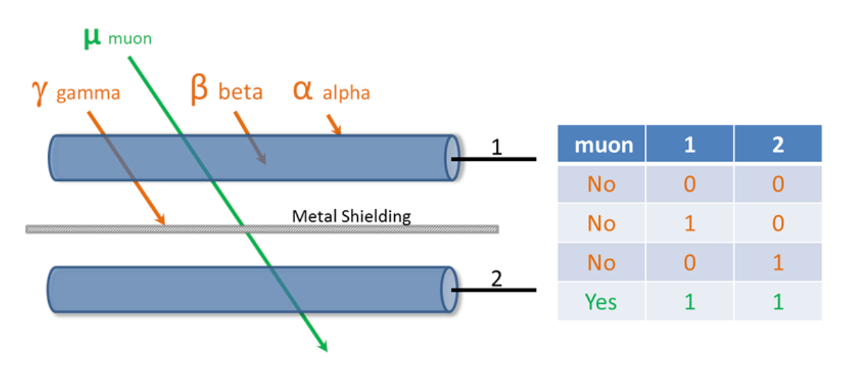
Figure 1: Illustration of the detector-coincidence concept to detect muons and filter out the signals from $\alpha$, $\beta$ and $\gamma$ radiation, that do not produce coincidences.

2.2 Description of the detector

The scintillator plus PMT setup comes already pre-assembled as a commercial detector unit (SCIONIX model R30*20B250/1.1-E3-P-X) which includes an Ej200 plastic scintillation detector of dimensions $20\times 30\times 250~{}$mm³ wrapped in reflector and surrounded by light tight vinyl coupled to 30 mm diameter R6094 PMT equipped with a voltage divider and counting electronics. The first 1.5 mm wrapping layer of this detector is not sensitive to radiation.

The detector has been built in a very compact setup for easy transportation and fits into a standard size “executive” suitcase (see Fig. 2). It is powered by a 12 V lead battery or alternatively connected to the 220 V AC electrical network. In this second case, the battery is recharged in parallel. From either the 12 V from the battery or the 220 V AC power supply delivering 12 V output, a power management circuitry delivers all the needed voltages (see Fig. 3).

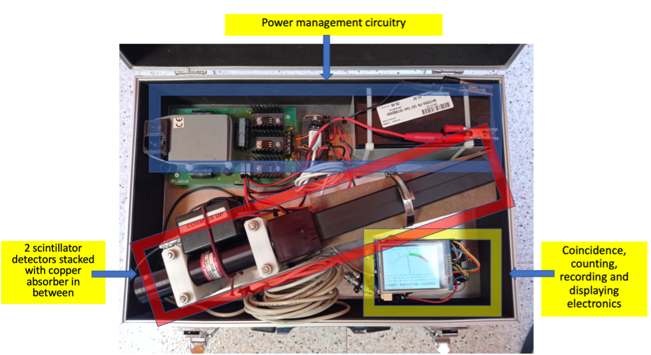
Figure 2: The muon detector inside the suitcase. The upper part is the power circuitry including the network inlet, the power supply and low voltage regulators, the HV generators and the lead battery for standalone operation without power connection. Below we positioned the two scintillator detector set stacked with a copper absorber in between. On the bottom-right, one finds the coincidence, counting, recording, and displaying circuitry.

Using DC-DC converters, from these 12 V the setup generates the high voltages needed to power the PMTs (700 V) and, using linear regulators, the 5 V needed to power the coincidence circuit and the microcontroller that takes care of the DAQ, displaying and recording.

Each scintillator plus PMT detector setup provides already a TTL digital discriminated output, that is used as input for the coincidence electronics. The length of the digital output is of 50 ns while the signal-overlap time requested for detecting a coincidence (resolving time) is of about 20 $\mu$s.

Each single detector signal, as well as their coincidences, are input to an Arduino Mega microcontroller that, using interrupts, counts them and computes their rate and their statistical uncertainty. The microcontroller also measures the setup temperature, humidity and atmospheric pressure and displays all the quantities mentioned into a large display while recording all that data into an SD card in easily readable text format for later analysis. The suitcase can be easily carried and installed in any place, while the battery provides an autonomy of a few days. Furthermore, it can easily incline to check the measured rates as a function of the zenith angle, as shown in Sec. 3.1.

2.3 Detector characterization

In order to assess the accidental coincidence rate $N_{a}$, one can use the single rate measurements $N_{i}$ from each detector together with the coincidence resolving time $\tau$ in a simple probabilistic calculation using the standard formula [52]:

$$N_{a}=2\tau\times N_{1}\times N_{2}.$$ (1)

In our detector, typical values measured for the single rates at ground level after taking data for about 20 hours are $N_{i}=701.57\pm 0.78$ CPM and, as mentioned before, $\tau=20\pm 2\,\,\mu$s, so that the calculated accidental coincidence rate is

$$N_{a}=0.33\pm 0.03\,\,\mathrm{CPM}.$$ (2)

Alternatively, for a direct measurement of the accidental rate the setup also allows a simple disassembly of the upper scintillator detector in such a way that it can be placed sideways, in a geometrical position in which the chances for any particle crossing both detectors are completely negligible (see Fig. 3). With this setup, the measured accidental rate at ground level after taking data for about 20 hours is

$$N_{a}=0.31\pm 0.02\,\,\mathrm{CPM}.$$ (3)

Therefore, both approaches give identical results within uncertainties.

The accidental rate is almost negligible (less than 1%) when compared with the typical coincidence rate at ground level $N_{c}$ after about 20 hours running,

$$N_{c}=40.00\pm 0.18\,\,\mathrm{CPM}.$$ (4)

For shallow and deep underground sites, this error becomes very relevant as it is comparable or larger than the actual reading (see Sec. 3.2).

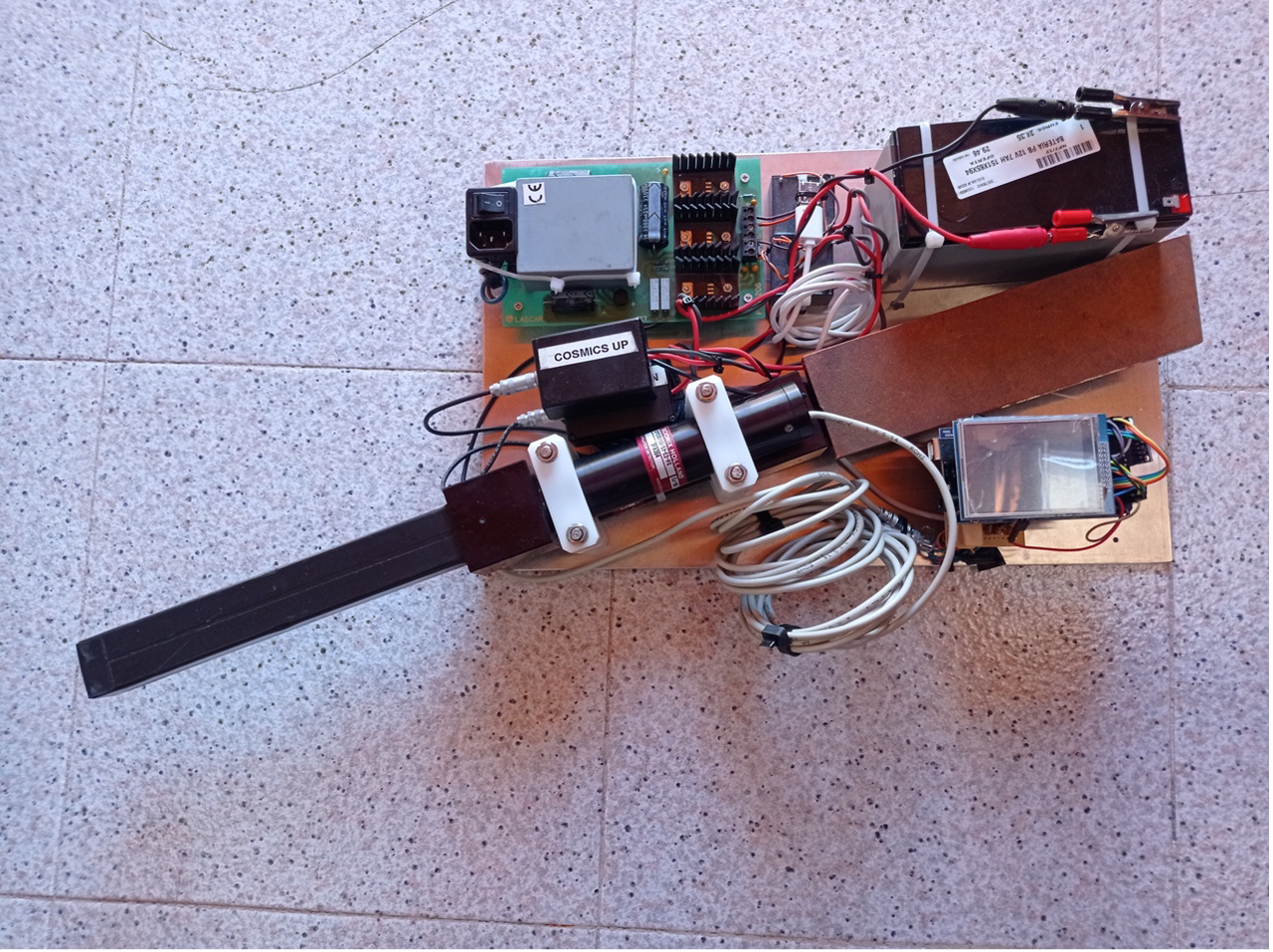
Figure 3: The muon detector setup for measuring the accidental coincidence rate. The upper scintillator detector set is turned 180 degrees in such a way that the geometrical overlap with the lower scintillator detector set is completely negligible .

3 Cosmic ray mitigation strategies

By employing the cosmic muon detector presented in the previous section, we demonstrate in this section different methods to lead to a smaller flux of cosmic muon counts, with a direct impact on superconducting qubit-based experiments.

3.1 Angular dependence of cosmic muon flux

The first mitigation strategy to reduce the total number of cosmic muon impacts on a device is to consider the angular dependence of the muon flux due to the absorption through the atmosphere.

In order to evaluate the flux of muons at sea level we use the aforementioned muon detector at varying orientations, this way measuring the muon flux at different zenith angles $\theta$, as shown in Fig. 4. The measurements are performed from an horizontal position $\theta=0$ of the detector looking directly at the sky overhead to a complete vertical one $\theta=\pi/2$ where the detector looks at the horizon (from both sides). The individual measurements are shown in Fig. 5, and they display a clear dependence on the detector orientation.

In order to fit the observed counts, the muon flux can be estimated roughly with a cosine law of the form $I(\theta)=I_{0}\cos^{2}(\theta)$ as shown by Bae, et al. [53]. However, here we require a more detailed model, which accounts for the finite thickness of the Earth’s atmosphere with the change of the zenith angle (see the Appendix 5.1 for more details). While the $I(\theta)$ law holds for a muon flux through an infinitesimal point in space for a certain incoming zenith angle $\theta$, the actual geometry of the detector needs to be accounted for.

The differential number of muons incident on a differential surface is given by

$$\mathrm{d}N=I(\theta)\,\mathrm{d}A\,\mathrm{d}\Omega\,\mathrm{d}t.$$ (5)

Here, $I(\theta)$ is the muon flux intensity, incident on the differential area $\mathrm{d}A$, over the solid angle $\mathrm{d}\Omega$, over a time $\mathrm{d}t$. In order to obtain the total rate of muon impacts $\Phi\equiv\Delta$N/$\Delta$t upon the detector one must integrate both over the angular aperture of the device and over its area:

$$\Phi(\theta)=\int_{\Omega}\int_{\mathrm{Area}}I(\theta)\,\mathrm{d}\Omega\,\mathrm{d}A.$$ (6)

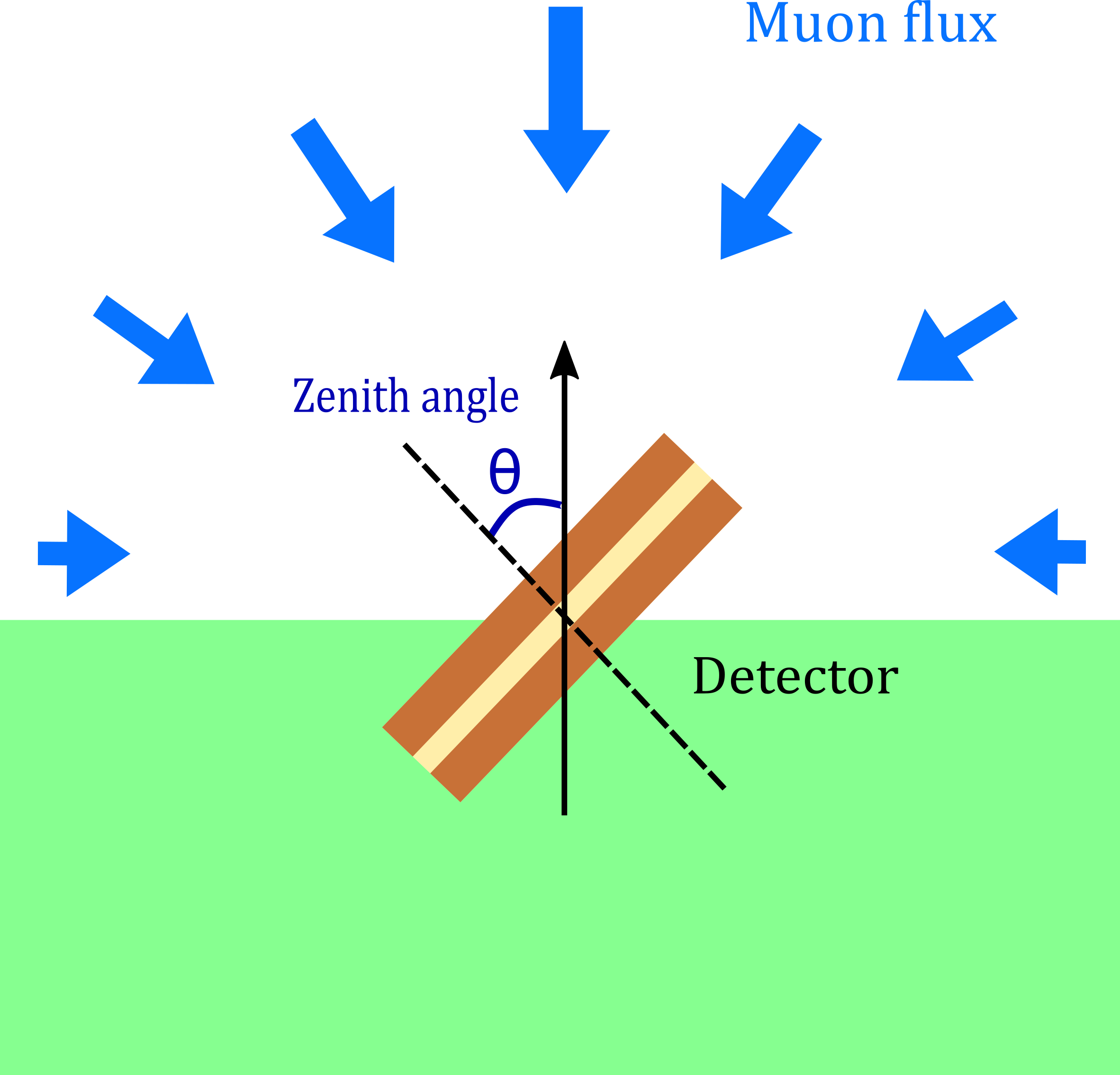
Figure 4: Depiction of the inclination of the muon detector, being oriented at anangle $\theta$ with respect to the zenith.

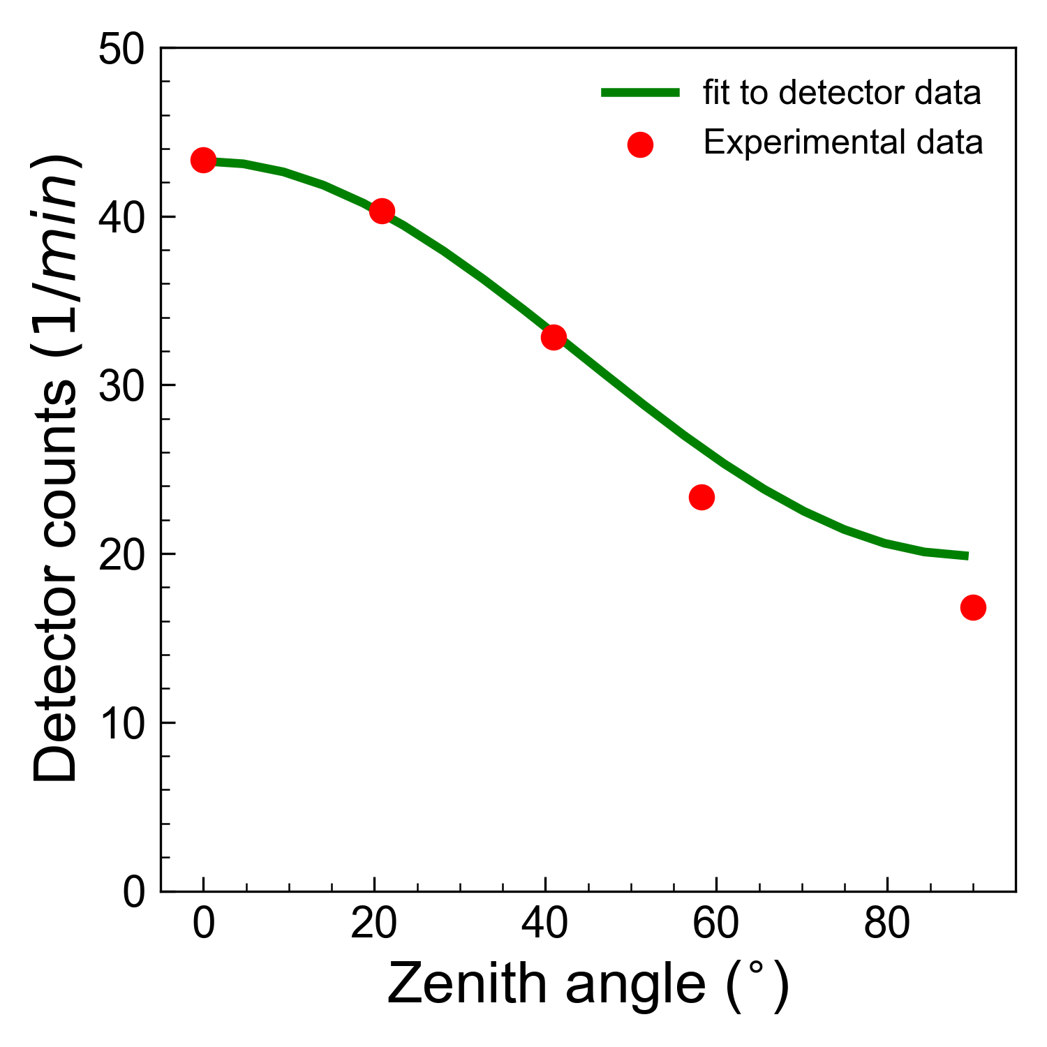
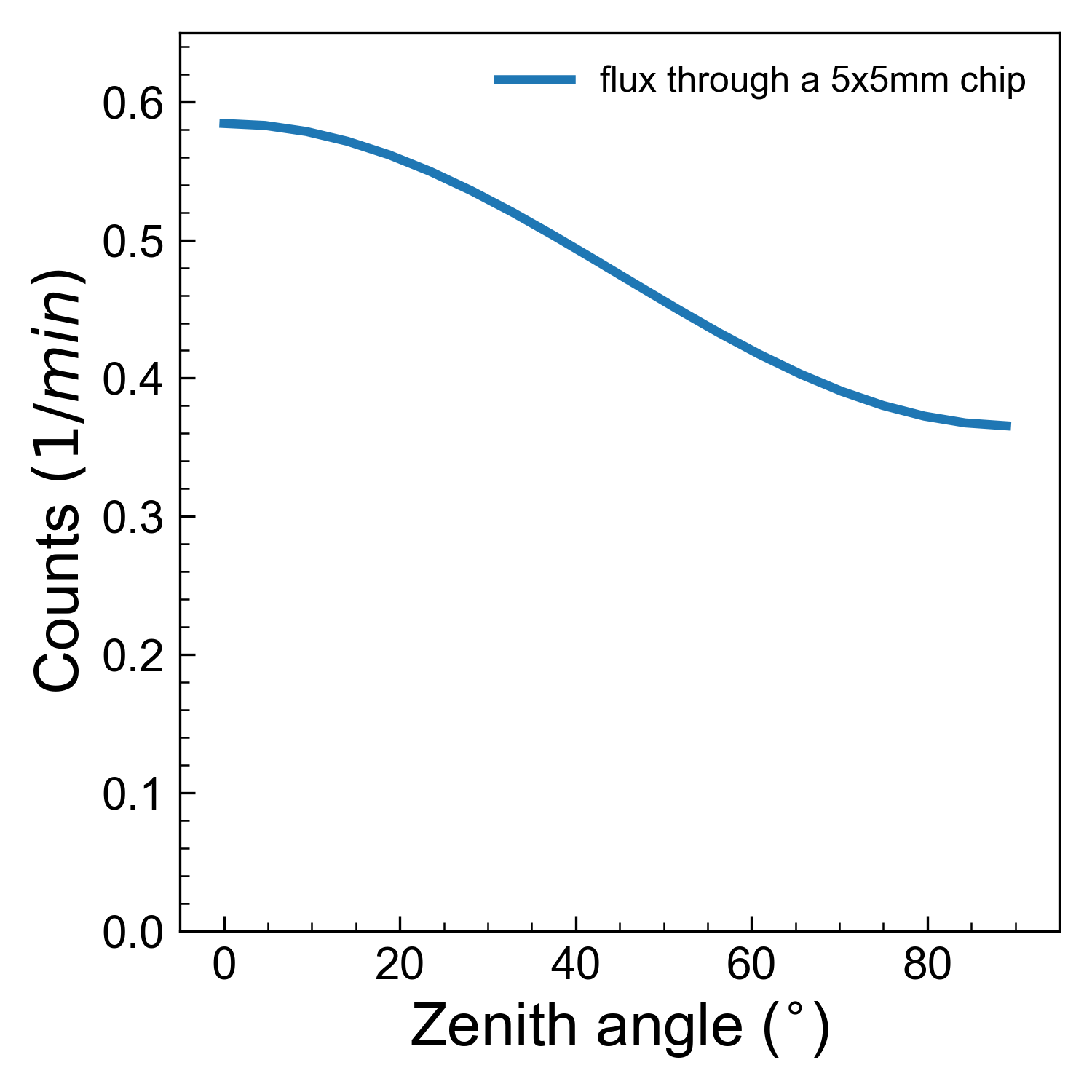
Figure 5: Muon flux as a function of the zenith angle. One the left we have experimental data for each measured angle and a fit using our model, Eq. (6). The fit is performed according to the corrected cosine-squared law (see Appendix). On the right, we apply the same model to deduce the muon impacts per minute for a typical chip of area $5\times 5$ mm², and $0.5$ mm thickness as a function of its inclination.

From the calculated angular flux dependence $\Phi(\theta)$, one obtains the total amount of cosmic muon impacts depending on the orientation of the detector. The result is plotted in Fig. 5 as the green trace. We use Eq. (6) to fit a muon flux intensity of $I_{0}=0.420$ cm^-2sr^-1min^-1, comparable to the work of Rossi [54], where $I_{0}=0.498$ cm^-2sr^-1min^-1 was obtained. The discrepancy may come from the lack of angular resolution from our detector due to the close proximity of the two scintillators.

Having validated our geometry-dependent muon flux model in Eq. (6), we can now use it to predict the angular dependence impinging on a typical qubit chip geometry. This is possible by using the exact same model as for our muon detector, but setting the aperture angles $\alpha$ and $\beta$ (defined in Appendix 5.3) of the detector to 180 degrees, which is equivalent to having one solid rectangular body. Taking a 0.5 mm thick silicon substrate with an area of $5\times 5$ mm² yields the result shown as the blue line on Fig. 5. A clear trend of decrease of the muon particle flux with the tilt of the device can be observed. Between $0^{\circ}$ and $90^{\circ}$ inclination, there is a decrease factor of $1.6$ in the muon rate. This demonstrates that the tilt of the device can impact the total amount of energy it receives from cosmic muons.

Based on these results, it is clear that, in order to minimize the cross-section with cosmic muons, superconducting qubit chips must be oriented with the surface looking towards the horizon.

3.2 Underground shielding

As explained in Sec. 1, experiments requiring the lowest possible noise background level locate their sensors in deep underground laboratories around the world, where the rock overburden screens most of the incoming cosmic radiation. Typical depths of underground laboratories are in the 1 km range, obtaining screening factors of cosmic muon flux of $10^{5}-10^{6}$ [55, 56]. Due to their remote location and scarcity, these underground stations do not represent a practical solution for improving the quality of any qubit type affected by cosmic rays. As the lifetime of superconducting qubits limited by ionizing radiation lies in the millisecond range for transmons [1], it may not be necessary to attain the screening factors achieved in deep underground laboratories and, instead, much shallower sites [14] may already offer a significant enough screening to bring qubit quality to a level desirable for applications such as error correction and sensing.

We have identified commonly-found locations in city environments providing significant screening factors from cosmic radiation. These are underground stations and side tunnels in underground highways. For the particular case of the city of Barcelona, we have conducted measurements in two such locations using our portable cosmic muon detector described in Sec. 2. The first site is the underground station ‘El Coll-La Teixonera’ located under a hill at a depth of approximately 100 meters (see Fig. 6).

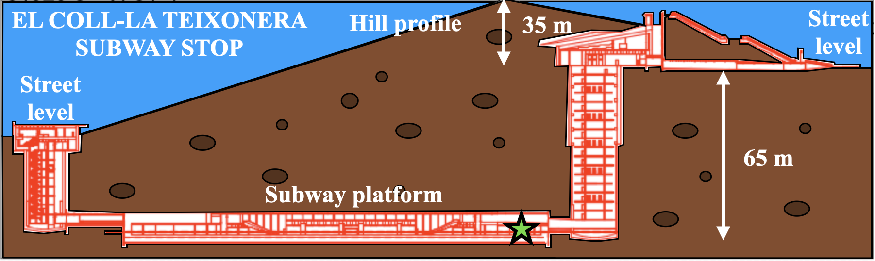
Figure 6: Profile of the TMB subway station ’El Coll-La Teixonera’ where measurements were conducted.

The second site is a side tunnel in an underground highway known as the Vallvidrera tunnels running under the ‘Collserola’ hill, with an approximated average depth of 120 m, with a peak height of 170 m (Fig. 7).

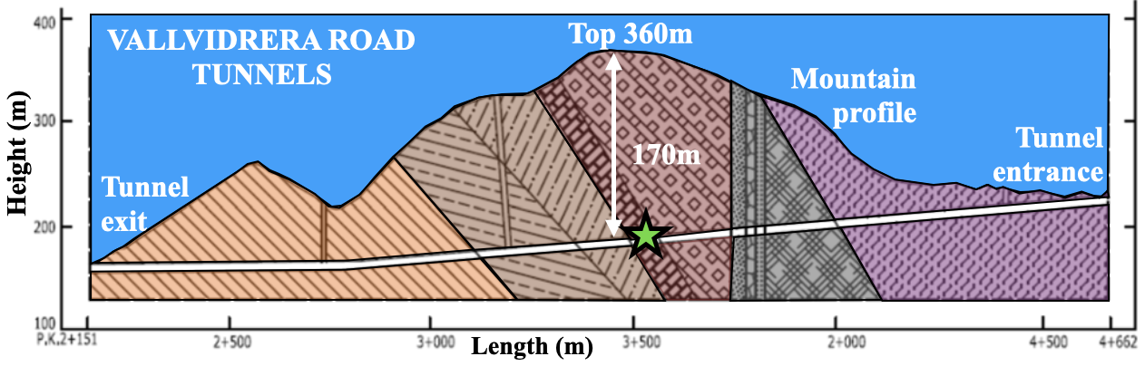
Figure 7: Profile of the Vallvidrera tunnel under the Collserola hill where measurements were conducted.

As a reference of a more realistic depth where qubit laboratories could be easily located, we also performed measurements in a much shallower site of 6 m in the sub-basement of the ALBA synchrotron located near the Bellaterra campus.

The results are shown in Fig. 8. All measurements were taken over 48 hours to minimize statistical uncertainty (smaller than the data markers in the plot). Above ground, we measure on average 40 CPM. The TMB and Vallvidrera shallow sites investigated display a muon count of 1.4 CPM and 1.1 CPM, respectively, achieving a screening factor of 29 and 36 with respect to ground. The 6 m shallower site achieves a rate of 20 CPM, representing a screening factor of 2. In all data, we have already subtracted the spurious coincidence counts from the apparatus dead time, as detailed in Sec. 2.3.

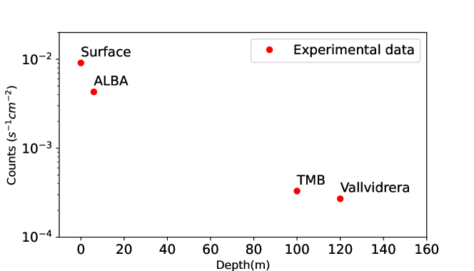
Figure 8: Measurement of muon counts as function of depth. The surface measurement is used as a reference for the two shallow underground sites identified: the Barcelona subway (TMB) and Vallvidrera tunnels. The ALBA synchrotron sub-basement is used as a typical laboratory location. The statistical uncertainty of all measurements is smaller than the marker size of the plot after averaging over 48h for each location.

For the case of the Vallvidrera tunnels, we have collected data for single events in our detector with the result of 1047.4 counts per minute. This represents a factor 1.68 higher than above ground in a usual office space, which is consistent with the presence of heavy minerals in the tunnels generating a higher amount of radioactivity. This is also consistent with measurements in deep underground laboratories. Therefore, it is necessary to equip qubit measurement setups with screening against this type of radioactivity, such as a lead shield. Note that given the low amount of cosmic ray flux in this shallow site, the re-excitation of lead isotopes detailed in Sec. 1.1 would take a much longer time scale than above ground.

Assuming one is able to screen environmental radioactivity using lead shielding, as is usual in underground sites, the screening factor obtained at 100 m depths would lead to a decrease of events to a level of $\sim 3\times 10^{-4}$ s^-1cm^-2. Using typical device dimensions for superconducting qubits of $\sim 1$ cm^-2, a device placed in such a shallow site would experience an average of 0.018 counts per minute, or 0.3 mHz, compared to 0.54 counts per minute, or 9 mHz, above ground.

4 Conclusions

In this work, we have provided two methods to reduce the flux of cosmic muons compatible with experiments involving superconducting qubits. The first method is to position the qubit chip pointing towards the horizon in order to minimize its cross section to incoming muons, this way reducing the flux a factor 1.6 above ground. The second method consists in locating qubit experiments in a shallow underground location, which could be as low as 10 m below surface. This small depth already provides strong protection against neutrons, and it reduces the cosmic muon flux by a factor 2. Deeper sites at 100 m depth would observe a reduction of cosmic muon flux on the order of 30. We have validated both methods using a home-built, portable cosmic muon counter consisting of two plastic scintillators integrated in a coincidence counting electronics circuit.

The unquestionable evidence of the effect of cosmic muons on qubits requires addressing this source of noise and instability with as much priority as the rest of sources of noise, such as TLS surface defects. Decreasing the impact of cosmic muons will only be possible through a combination of techniques to reduce their flux, following methods similar to the ones proposed in this work, and their impact with on-chip mitigation techniques, such as phonon and quasiparticle suppression. Understanding the physics of cosmic muons interacting with qubit devices is an important future step to further suppress their effect and lead to higher quality qubits to build more robust quantum computers and more stable quantum sensors.

5 Appendix

5.1 Correction to the $\cos^{2}\theta$ law

In order to take into account the Earth’s curvature radius, and hence the real atmosphere thickness as a function of zenith angle in the expectation of the angular dependence of the muon flux, Fig. 9 shows the actual geometrical dependence. There, $r$ stands for Earth’s radius (about 6400 km), $a$ stands for the vertical atmosphere thickness (taken to be 10 km), $\theta$ is the zenith angle and $p$ the atmosphere thickness at that zenith angle.

After applying some geometrical considerations, we obtain an expression for the Earth’s atmosphere crossed by muons $p(\theta)$ as a function of the zenith angle $\theta$ as follows:

$$p(\theta)=-r\cos(\theta)+\sqrt{a^{2}+2ar+[r\cos(\theta)]^{2}}.$$ (7)

For small angles near $0$, we recover $p\simeq a$, as expected. For horizontal zenith (90 degrees) and since $r\gg a$, then $p\simeq\sqrt{2ar}\gg a$.

Since the muon flux decreases due to the atmosphere’s absorption, it should be inversely proportional to the square of the atmosphere’s thickness, namely to the square of $p$. This correction shall therefore be taken into account to the fit of our data, particularly when comparing the results for vertical (0 degrees zenith) and horizontal (90 degrees zenith) muon fluxes.

Thus, the following expression for the flux is obtained:

$$I(\theta)=I_{0}\left(\frac{a}{-r|\cos(\theta)|+\sqrt{a^{2}+2ar+[r\cos(\theta)]^{2}}}\right)^{2}.$$ (8)

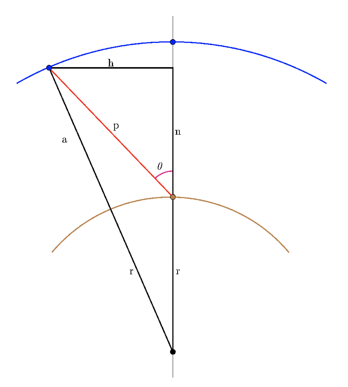
Figure 9: A model of planet Earth and its atmosphere. The radius $r$ of the planet is taken to be 6400 km. The atmosphere thickness $a$ is taken to be 10 km. $\theta$ is the zenith angle and $p$ portrays the thickness of the atmosphere at an angle $\theta$, which is the one crossed by incoming muons.

5.2 The zenith angle definition

The area of the sky our detector looks at is a spherical rectangle (a rectangle projected on a sphere). This area takes a big part of the surface of the unit sphere one integrates over and thus it also crosses the poles of the sphere, where one encounters a discontinuity. In order to avoid that discountinuity, we make a change in the reference system. Instead of the detector rotating with respect to the sky, we have the sky rotate with respect to the detector (by an amount $\theta_{zenith}$, which spans the range$[0,\pi/2]$), while the detector is fixed facing in direction of the equator (the normal vector of the detector stays on the $x-y$ plane). On Fig. 10 one can see the spherical coordinate system used for integration.

The zenith angle transformed will thus be:

$$\theta_{\mathrm{mod}}(\theta_{\mathrm{zenith}},\theta,\phi)=\arcsin[\sin(\theta_{\mathrm{zenith}}+\theta)\cos(\phi/2)].$$ (9)

Here, $\theta_{mod}$ is the angle of deviation from the normal of the detector surface (which is aligned with the $x$-axis, see Fig. 10).

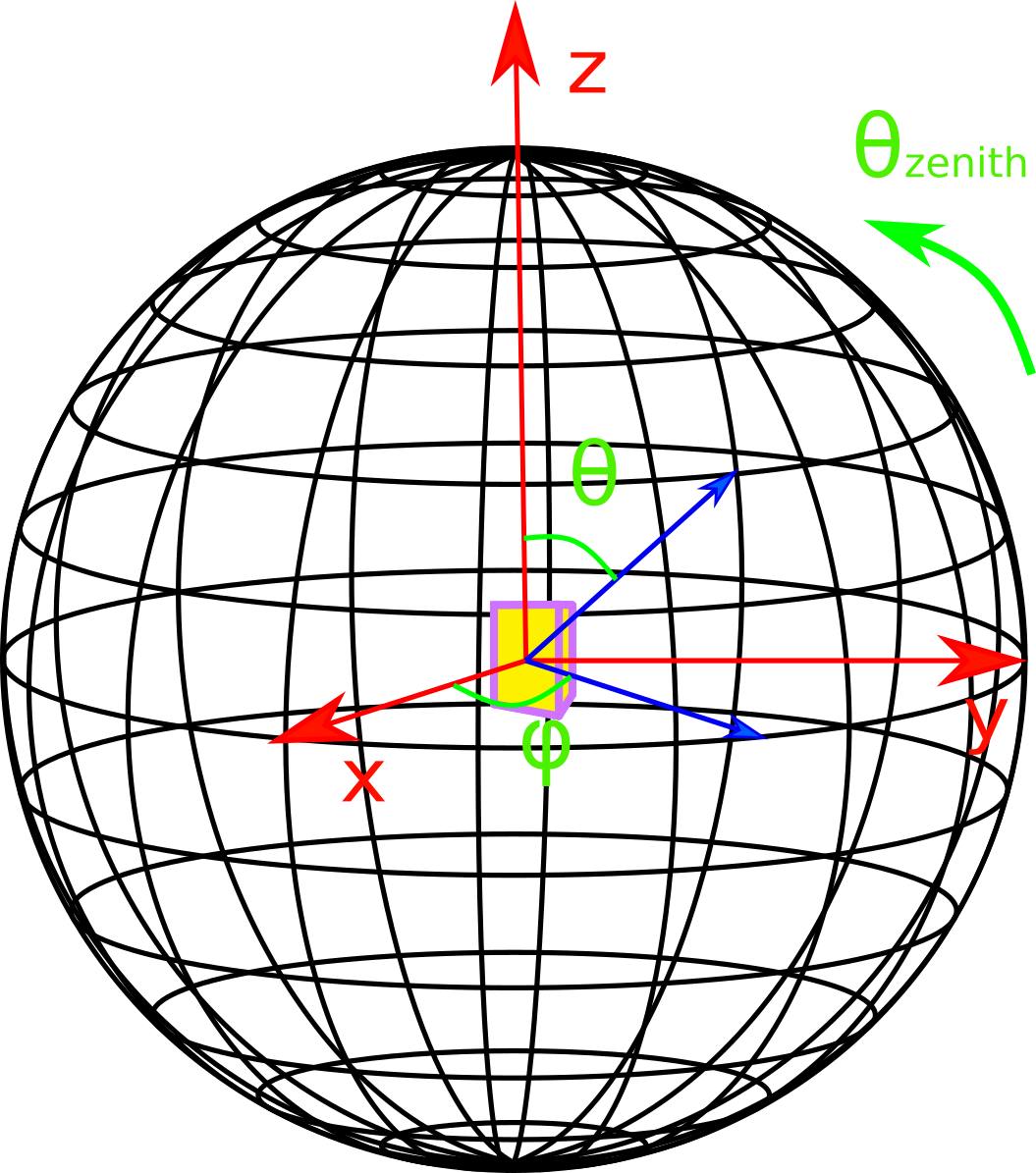
Figure 10: The spherical coordinate system.

5.3 The area correction

The geometry of our detector also needs to be accounted for when constructing the model. This is because for a particle to be registered as a muon it must penetrate both scintillators. However, the angles at which this can be accomplished are limited by the geometry of the detector itself, as shown in Fig. 11. Also, the effective area seen by particles coming with a certain inclination angle with respect to the detector will be a function of this inclination angle, as illustrated in Fig. 11.

Our particular detector is a rectangular cuboid with height $h$, width $W$ and length $L$. The area of the detector is defined by $A=L\times W$. After the correction for the area, the effective area becomes $A^{\prime}=L^{\prime}\times W^{\prime}$, where we define $L^{\prime}$ and $W^{\prime}$ as:

$$L^{\prime}=L-h|\tan(\theta)|\quad,\mathrm{where}\quad\theta\in[-\alpha/2,\alpha/2]$$ (10)

$$W^{\prime}=W-h|\tan(\phi)|\quad,\mathrm{where}\quad\phi\in[-\beta/2,\beta/2]$$ (11)

Here, the $\theta$ and $\phi$ are the zenith and azimuth angles, respectively, and they sweep values within the aperture angles for the length side $-\alpha$ and the width side $-\beta$, respectively [Fig 11 and Fig 12].

The aperture angles are calculated as follows:

$$\alpha=2\arctan(L/h).$$ (12)

$$\beta=2\arctan(W/h).$$ (13)

Our scintillators have dimensions $L=24.7$ cm, $W=2.7$ cm, $h=1.7$ cm.

The aperture angles ultimately express the fact that the two scintillators have a gap in between them. Because the detection of a muon happens when a particle is detected to pass trough both scintillators consecutively, if a particle comes at such as steep angle that cannot pass through both scintillators, but only trough one or none of them, it won’t be detected. This steep angle defines the range of detection of the scintillators and thus defines their aperture, how much does the detector ”see” (in terms of solid angle), as shown in Fig. 11. If one increases the distance between the scintillators, the aperture angle decreases. If the distance between them is zero, then the aperture angle becomes 180 degrees and it allows to simulate a solid structure, such as a rectangular chip as used to plot the curve in Fig. 5 of the main text.

Finally, note that the angular dependence experiment was conducted at the campus of Autonomous University of Barcelona, located in a basin surrounded by buildings and hills. To avoid the screening effect of the surrounding environment, we neglected the shallowest 15 degrees over the horizon when we calculate the integral of the total flux in Fig. 5.

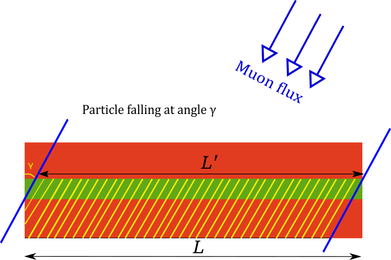
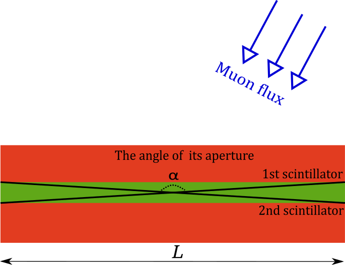
Figure 11: The left figure shows the variation of the effective detector area as function of the incident angle of the incoming muons. The same consideration applies to the other side of the rectangular cuboid. The right figure defines an aperture angle $\alpha$. All particles which fall on the detector at angles steeper then $\alpha/2$ will not be registered.

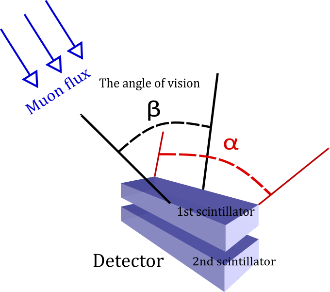
Figure 12: The aperture angles of the detector.

5.4 The final expression for the muon rate

The expression used to model our particular detector is:

$$\Phi(\theta_{\mathrm{mod}})=\int_{-\alpha/2}^{\alpha/2}\int_{-\beta/2}^{\beta/2}I(\theta_{\mathrm{mod}})A^{\prime}(\theta,\phi)\sin(\theta)\,\mathrm{d}\theta\,\mathrm{d}\phi.$$ (14)

This expression and can be used for any class of similar detectors. Here, we use the expressions in Eqs. (8)–(11).

References

- [1] A. P. Vepsäläinen et al., Nature 584, 551 (2020).
- [2] L. Cardani et al., Nature Communications 12, 2733 (2021).
- [3] CDMS, D. Abrams et al., Phys. Rev. D 66, 122003 (2002), astro-ph/0203500.
- [4] C. Arnaboldi et al., Nuclear Instruments and Methods in Physics Research Section A: Accelerators, Spectrometers, Detectors and Associated Equipment 518, 775 (2004).
- [5] G. Angloher et al., Astropart. Phys. 31, 270 (2009), 0809.1829.
- [6] SuperCDMS, R. Agnese et al., Phys. Rev. D 95, 082002 (2017), 1610.00006.
- [7] R. T. Gordon et al., Applied Physics Letters 120, 074002 (2022), https://doi.org/10.1063/5.0078785.
- [8] M. McEwen et al., Nature Physics 18, 107 (2022).
- [9] T. Thorbeck, A. Eddins, I. Lauer, D. T. McClure, and M. Carroll, arXiv:2210.04780 (2022).
- [10] V. Iaia et al., Nature Communications 13, 6425 (2022).
- [11] F. Henriques et al., Applied Physics Letters 115, 212601 (2019), https://doi.org/10.1063/1.5124967.
- [12] R.-P. Riwar et al., Phys. Rev. B 94, 104516 (2016).
- [13] A. ”Bargerbos et al., arXiv:2207.12754 (2022).
- [14] C. E. Aalseth, Review of Scientific Instruments 83 (2012).
- [15] A. Langenkämper, Journal of Low Temperature Physics 193, 860–866 (2018).
- [16] F. G. Schröder, Prog. Part. Nucl. Phys. 93, 1 (2017), 1607.08781.
- [17] A. Letessier-Selvon and T. Stanev, Rev. Mod. Phys. 83, 907 (2011), 1103.0031.
- [18] Particle Data Group, R. L. Workman, PTEP 2022, 083C01 (2022).
- [19] P. L. Rocca, D. L. Presti, and F. Riggi, Cosmic ray muons as penetrating probes to explore the world around us, in Cosmic Rays, edited by Z. Szadkowski, chap. 3, IntechOpen, Rijeka, 2018.
- [20] A. Bettini, Eur. Phys. J. Plus 127, 114 (2012).
- [21] J. W. Beeman et al., Appl. Radiat. Isot. 194, 110704 (2023), 2206.05116.
- [22] J. A. Formaggio and C. J. Martoff, Ann. Rev. Nucl. Part. Sci. 54, 361 (2004).
- [23] S. Cebrián, Int. J. Mod. Phys. A 32, 1743006 (2017), 1708.07449.
- [24] C. Zhang, D. M. Mei, V. A. Kudryavtsev, and S. Fiorucci, Astropart. Phys. 84, 62 (2016), 1603.00098.
- [25] V. V. Kuzminov, Eur. Phys. J. Plus 127, 113 (2012).
- [26] A. Murphy and S. Paling, Nuclear Physics News 22, 19 (2012).
- [27] A. Bettini, Eur. Phys. J. Plus 127, 112 (2012).
- [28] CUPP, J. T. Peltoniemi, AIP Conf. Proc. 533, 18 (2000).
- [29] L. Votano, Eur. Phys. J. Plus 127, 109 (2012).
- [30] F. Piquemal, Eur. Phys. J. Plus 127, 110 (2012).
- [31] J.-P. Cheng et al., Ann. Rev. Nucl. Part. Sci. 67, 231 (2017), 1801.00587.
- [32] Y. Suzuki and K. Inoue, Eur. Phys. J. Plus 127, 111 (2012).
- [33] J. Heise, J. Phys. Conf. Ser. 606, 012015 (2015), 1503.01112.
- [34] K. T. Lesko, AIP Conf. Proc. 1672, 020001 (2015).
- [35] E.-I. Esch et al., Nucl. Instrum. Meth. A 538, 516 (2005), astro-ph/0408486.
- [36] S. MacMullin, AIP Conf. Proc. 1338, 78 (2011).
- [37] N. J. T. Smith, Eur. Phys. J. Plus 127, 108 (2012).
- [38] An Assessment of the Deep Underground Science and Engineering Laboratory (DUSEL).
- [39] J. M. Martinis, npj Quantum Information 7, 90 (2021).
- [40] G. Catelani et al., Phys. Rev. Lett. 106, 077002 (2011).
- [41] J. Lisenfeld et al., npj Quantum Information 5, 105 (2019).
- [42] M. Neeley et al., Nature Physics 4, 523 (2008).
- [43] P. V. Klimov et al., Phys. Rev. Lett. 121, 090502 (2018).
- [44] A. G. Fowler, M. Mariantoni, J. M. Martinis, and A. N. Cleland, Phys. Rev. A 86, 032324 (2012).
- [45] S. N. Dorenbos et al., Applied Physics Letters 98, 251102 (2011).
- [46] C. D. Wilen et al., Nature 594, 369 (2021).
- [47] I. M. Pop et al., Nature 508, 369 (2014).
- [48] A. Somoroff et al., arXiv:2103.08578 (2021).
- [49] X. Pan et al., Nature Communications 13, 7196 (2022).
- [50] L. Cardani et al., arXiv:2211.13597 (2022).
- [51] K. Karatsu et al., Applied Physics Letters 114, 032601 (2019), https://doi.org/10.1063/1.5052419.
- [52] L. Jánossy, Nature 153, 165 (1944).
- [53] J. Bae, S. Chatzidakis, and R. Bean, International Conference on Nuclear Engineering 85277, V004T14A011 (2021).
- [54] B. Rossi, Rev. Mod. Phys. 20, 537 (1948).
- [55] W. H. Trzaska et al., arXiv:1902.00868 (2019).
- [56] G. Bellini and et al., JCAP 05, 015 (2012).