Configuration-specific insight to single-molecule conductance and noise data revealed by principal component projection method

Zoltán Balogh,^a,b Gréta Mezei,^a,b Nóra Tenk,^a András Magyarkuti,^a and András Halbritter^∗a,b

^a Department of Physics, Institute of Physics, Budapest University of Technology and Economics, Műegyetem rkp. 3., H-1111 Budapest, Hungary. E-mail: halbritter.andras@ttk.bme.hu
^b ELKH-BME Condensed Matter Research Group, Műegyetem rkp. 3., H-1111 Budapest, Hungary.

We explore the merits of neural network boosted, principal-component-projection-based, unsupervised data classification in single-molecule break junction measurements, demonstrating that this method identifies highly relevant trace classes according to the well-defined and well-visualized internal correlations of the dataset. To this end, we investigate single-molecule structures exhibiting double molecular configurations, exploring the role of the leading principal components in the identification of alternative junction evolution trajectories. We show how the proper principal component projections can be applied to separately analyze the high or low-conductance molecular configurations, which we exploit in $1/f$-type noise measurements on bipyridine molecules. This approach untangles the unclear noise evolution of the entire dataset, identifying the coupling of the aromatic ring to the electrodes through the $\pi$ orbitals in two distinct conductance regions, and its subsequent uncoupling as these configurations are stretched.

1 Introduction

The field of single-molecule electronics (SME) has developed a broad range of experimental methods to gain insight to the properties of the ultimate smallest conductors, where a single molecule bridges two metallic electrodes.^{1, 2, 3, 4, 5} The creation of single-molecule nanowires heavily relies on the so-called break junction methods, where the fine mechanical rupture of a metallic nanowire is utilized first to establish a single-atom metallic nanojunction, and afterwards to contact a single-molecule between the two apexes of a broken atomic junction.^{6, 1, 2, 4, 7} The basic output of the break junction measurements is a statistical ensemble of conductance vs. electrode separation traces, from which the fingerprints of the single-molecule configurations can be visualized on conductance histograms. This analysis is frequently extended by more delicate experimental methods, like force,^{2, 8, 9, 10, 11} noise,^{12, 13, 14, 15, 16, 11, 17, 18, 19, 20, 21, 22} thermoelectric power,^{2, 23, 24} thermal conductance,^{25, 26, 27} quantum conductance fluctuation^{28, 29} or superconducting subgap spectroscopy measurements.^{30, 31} The combination of such methods was found to be extremely efficient in resolving the fine details of the structural and electronic properties of single-molecule nanowires.

In spite of this broad range of diagnostic tools, single-molecule electronics still suffers from the diversity of the data, i.e. the formation of a broad range of various single-molecule configurations during the repeated opening and closing of the junction. Conductance histograms are sufficient to resolve the conductance of the most probable molecular configurations. However, if a deeper insight is required, or further properties are also analyzed in parallel with the conductance data, it is useful to filter out the traces indeed reflecting the molecular configuration under focus, otherwise, the mixture of alternative configurations in the dataset may obscure the result of the analysis. This kind of data filtering is a traditional ingredient of break junction data analysis mostly relying on well-defined, but custom-created filtering algorithms.^{32, 33, 34, 35} The recent progress of machine learning (ML) based data analysis has brought a novel perspective to the field of SME as well.^{36, 37, 38, 39, 40, 41, 42, 43, 44, 45} However, in this field the widespread supervised ML approaches are less favored, as pre-labeled example traces are usually not available, and the manual selection of training traces is also unreliable and unwanted. Instead, the unsupervised identification of the relevant trace classes is desired, which is indeed possible by proper ML approaches, including reference-free clustering methods, or auto-encoder-based clustering.^{37, 38, 40, 41, 42, 46}

Here we examine an alternative unsupervised feature recognition approach relying on the internal correlations of the dataset. This method utilizes the cross-correlation analysis of the conductance traces.^{47, 48, 49, 33, 50, 45} The leading principal components (PCs), i.e. the most important eigenvectors of the 2D correlation matrix identify the most relevant correlations in the dataset offering a unique tool for the efficient identification of the relevant trace classes. The principal component projection (PCP) method was first introduced and successfully applied to identify artificially mixed traces of different molecules.⁵¹ Later, the authors of this paper demonstrated the sorting of molecular and tunneling traces by PCP method.⁵² In the latter work, it was also shown that the classification accuracy is significantly improved if the PCPs are only used to automatically generate the most characteristic traces for the two trace classes, which are then used as the training dataset of a simple neural network (NN).⁵²

Inspired by the initial success of the PCP approach, here we further exploit this method via the analysis of room-temperature Au–4,4’-bipyridine (BPY)–Au^{7, 53, 54, 55, 56, 57, 52, 58, 45} and Au–2,7-diaminofluorene (DAF)–Au¹¹ molecular nanowires. Both systems exhibit two different molecular configurations, i.e. alternative junction evolution trajectories are conceivable. We demonstrate that all the leading principal components provide highly relevant classification criteria, i.e. the PCP method is indeed an efficient and robust data filtering tool to recognize the alternative trace classes, which are mixed in the entire dataset. This can be harvested in more complex single-molecule measurements, where a configuration-specific insight into the data is desired. The latter is demonstrated by our PCP-aided, configuration-specific $1/f$-type noise measurements on BPY single-molecule junctions. These measurements investigate the scaling of $1/f$-type noise amplitude with the junction conductance, which is a specific device fingerprint distinguishing through-bond and through-space molecular coupling.^{14, 12, 11, 18, 21} In the latter case, a weak bond is involved in the transport, where tiny distance fluctuations exponentially convert to a significant conductance noise. This yields conductance independent relative conductance noise, $\Delta G/G$ similar to a tunnel junction, where the exponential dependence of the conductance on the distance, $G\sim\exp(-\beta\cdot d)$ converts to $\Delta G/G\sim\mathrm{const.}$ for a constant $\Delta d$ distance fluctuation.^{14, 12} As a sharp contrast, in case of through-bond coupling a strong chemical bond fixes the molecule-apex distance, and therefore the noise is not related to distance fluctuations in the bond, rather to close-by atomic fluctuations of the metallic apex. This phenomenon results in a definite increase of the relative conductance noise with decreasing junction conductance yielding a scaling exponent close to $\Delta G/G\sim G^{-0.5}$.^{14, 12} Our noise analysis on BPY molecules yields a complex, unclear $\Delta G/G$ vs. $G$ dependency. The PCP-based configuration-specific noise analysis, however, fully clarifies the noise characteristics of the two distinct molecular configurations, providing a refined insight to the bond evolution.

2 Results and Discussion

Basics of the measurements. The break junction measurements are performed by scanning tunneling microscope (STM) or mechanically controllable break junction (MCBJ) methods, where the mechanically sharpened Au tip of a custom-designed STM setup is brought into contact with a gold thin film sample covered by the target molecules, or a gold wire is broken in molecular environment using a three-point bending geometry.¹ In both cases, the rupture and the closing of the junction is repeated several thousand times, characterizing each rupture process by a conductance vs. electrode separation ($G(z)$) trace. From each measured trace, indexed with $r$, a single-trace histogram denoted by $N_{i}(r)=N(G_{i},r)$ is calculated by dividing the conductance axis to discrete bins ($G_{i}$) - and counting the number of data points in each bin. The conductance histogram of the entire dataset, $\left<N_{i}(r)\right>_{r}$ is obtained by averaging the single-trace histograms for all traces. These simple conductance histograms can be expanded to two-dimensional conductance histograms,^{59, 53} where the displacement information is also visualized. The such-obtained one-dimensional and two-dimensional conductance histograms for room-temperature Au-BPY-Au and Au-DAF-Au single-molecule junctions are presented in Figs. 1a,b (BPY) and Figs. 1d,e (DAF) (see the blue area graphs in the 1D histograms). In both cases, the formation of single-atom Au junctions is reflected by a sharp peak at the quantum conductance unit, $G_{0}=2e^{2}/h$, and both molecular systems exhibit double molecular configurations, one with higher and one with lower conductance (HighG/LowG). In the case of BPY, it is suggested that at a smaller electrode separation, the molecule can bind such that both the nitrogen linker and the aromatic ring is electronically coupled to the electrode, yielding a higher (HighG) single-molecule conductance (Fig. 1g1). Upon further pulling, the molecule slides to the apex and only the linkers couple to the electrodes (Fig. 1g2) yielding a decreased (LowG) conductance value. ^{53, 54, 55, 60} In the case of DAF the HighG/LowG configurations are interpreted as monomer/dimer molecular junctions (see Figs. 1h1,h2).¹¹

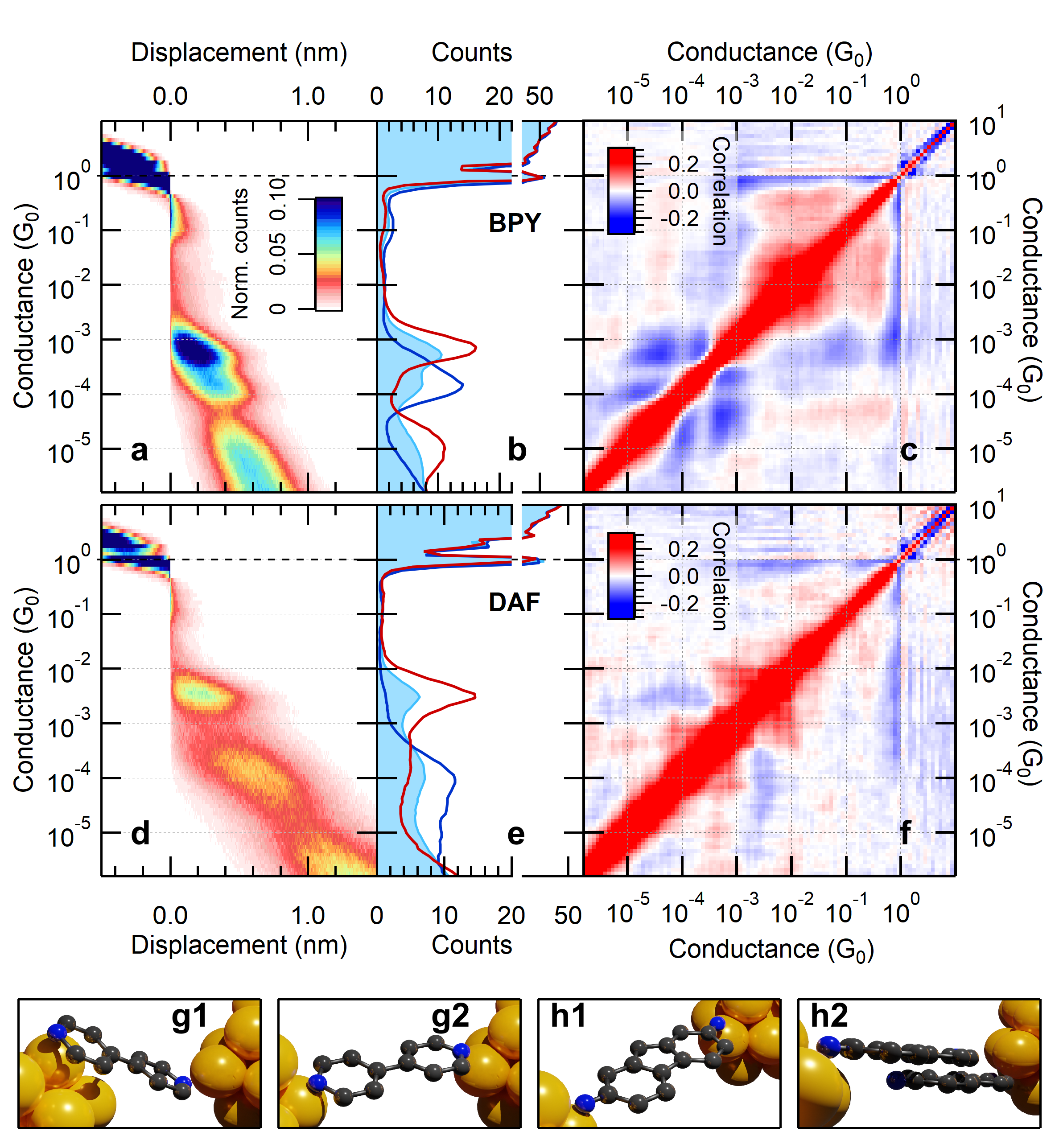
Figure 1: Histograms and correlation plots of BPY and DAF molecules. The top row represents the characteristics of BPY molecules, including the 2D histogram (a), the 1D histogram (blue area graph in panel (b)), and the $C_{i,j}$ correlation plot (c). The red and blue lines in panel (b) represent the histograms of the data subsets obtained by EPCP analysis (see text). The second row similarly demonstrates the 2D histogram (d), the 1D histogram (e), and the correlation plot (f) for DAF molecules. On the 2D histograms the origin of the displacement axis is set to the position, where the conductance trace crosses $G_{\mathrm{ref}}=0.5\,$G₀. Panels g1 and g2 illustrate the hypothesized HighG and LowG BPY configurations, whereas h1 and h2 illustrate the HighG (monomer) DAF configuration and the LowG (dimer) DAF configuration.

Basics of principle-component-projection-based conductance trace classification. The one- and two-dimensional conductance histograms represent an average behavior of the conductance traces. However, further, highly relevant information is obtained from the correlation matrix of the dataset,^{47, 48} highlighting the correlated deviations from the average behavior:

$$C_{i,j}=C(G_{i},G_{j})=\frac{\left<(N_{i}(r)-\left<N_{i}(r)\right>)\cdot(N_{j}(r)-\left<N_{j}(r)\right>)\right>}{\left<(N_{i}(r)-\left<N_{i}(r)\right>)^{2}\right>\cdot\left<(N_{j}(r)-\left<N_{j}(r)\right>)^{2}\right>}.$$

The correlation matrices of the Au-BPY-Au and Au-DAF-Au systems are demonstrated in Figs. 1c,f, both exhibiting a rich correlation structure. Some aspects of the correlation matrix can be interpreted with proper experience,^{47, 48, 49, 33, 50, 45} but the complexity of analyzing 2D correlation matrices is significantly reduced by concentrating on the most important correlations represented by the $P_{i}^{(n)}$ principal components, i.e. the eigenvectors of the correlation matrix.⁵¹ Here, the $n$ label sorts the principal components according to the descending order of the corresponding eigenvalue.

The principal component projection of a certain conductance trace is obtained as $PCP^{(n)}(r)=\sum_{i}P_{i}^{(n)}\cdot N_{i}(r)$, i.e. the scalar product of the principal component and the single-trace histogram. According to the proposal of J. Hamill and coworkers, the $PCP^{(n)}(r)\lessgtr 0$ relation can be used to sort the traces to two relevant trace classes.⁵¹ This idea was successfully applied to separate artificially mixed traces of two different molecular systems. It was also shown that the zero PCP value is not necessarily the proper threshold for the selection, and the accuracy of PCP-based data classification can be further refined by relying only on the traces with the largest positive/negative PCP (e.g. selecting $20\%-20\%$ of all traces).⁵² If the classification of the entire dataset is not targeted, solely the traces with these extreme principal component projection (EPCP) can be considered as a subset of the traces best representing some distinct behavior. Alternatively, these characteristic traces can be applied as the training dataset for a simple double-layer feed-forward neural network.⁵² In this combined PCP-NN method the neural network learns the important features from these training traces, and then generalizes for traces with less obvious characters. The decision-making process of this simplest possible neural network is well-represented by the so-called summed weight product,⁵² $SWP_{i}=\sum_{j}W^{(1)}_{i,j}\cdot W^{(2)}_{j}$, where $W^{(1)}_{i,j}$ / $W^{(2)}_{j}$ is the neural weight matrix / vector between the input layer and the hidden layer / hidden layer and output neuron of the NN, respectively. If $SWP_{i}$ is a large positive / negative number for a certain input, a large input value (i.e. a large histogram count) pushes the decision towards one or the other selection group.

Principle component projection analysis of room-temperature bipyridine and diaminofluorene single-molecule junctions. In our previous work the PCP-NN method was successfully applied in low-temperature single-molecule measurements,⁵² where the molecular pick-up rate was relatively low, and therefore, it was a primary task to separate molecular and non-molecular (tunneling) traces. In the following, we further demonstrate the merits and constraints of the EPCP and the combined PCP-NN method by analyzing the trace classes according to all the leading principal components in room-temperature measurements with BPY and DAF molecules. These measurements exhibit $\approx 100\%$ molecular pick-up rate, and therefore, instead of molecular/tunneling distinction, we rather focus on the analysis of the possible relations of the LowG and HighG molecular configurations. The results of the EPCP analysis are illustrated in Figs. 1b,e for a highly relevant principal component. The red / blue curves show the conductance histograms for the traces with the largest positive / negative principal component projection, relying on $P^{(3)}$ ($P^{(2)}$) for BPY (DAF) molecules. All selections include $20\%$ of all traces, and for both molecules, one selection exhibits the dominance of the HighG configuration and the suppression of the LowG configuration, and the other selection behaves vice versa. The possibility of this separation is already surprising, as the 2D histograms of both molecular systems (Figs. 1a,d) suggest that first the HighG configuration appears, and the LowG configuration only forms upon further stretching. This scenario would imply that the LowG configuration appears together with the HighG one. As a very sharp contrast, the EPCP method demonstrates, that one can find a significant portion (in this case $20\%$) of the traces, where the pronounced LowG peak can be observed without any significant HighG weight. This means that the average behavior represented by the 1D and 2D histograms may obscure possible highly relevant junction evolution trajectories, which can be, however, uncovered by the proper principal component projection.

Further on, we extend the EPCP method by the neural network supplement and analyze the such obtained trace classes for the four leading principal components in room-temperature Au-BPY-Au junctions (Fig. 2). The rows of the figure respectively represent the analysis according to the first, second, third, and fourth principal components. For a certain principal component, the separated two trace classes are demonstrated both by 2D conductance histograms (Figs. 2a1-a4 and b1-b4), and by 1D conductance histograms (Figs. 2c1-c4). In the latter case, the light blue background histogram represents the reference histogram for the whole dataset, whereas the red and blue lines demonstrate the histograms of the two datasets obtained by the PCP-NN analysis. In the fourth column (Figs. 2d1-d4) the actual principal component (dark green lines), and the summed-weight products of the neural network (light green lines) are demonstrated. Naturally, the selected one / other trace class exhibits pronounced weights in those conductance regions, where the PC and the SWP exhibit large positive / negative values.

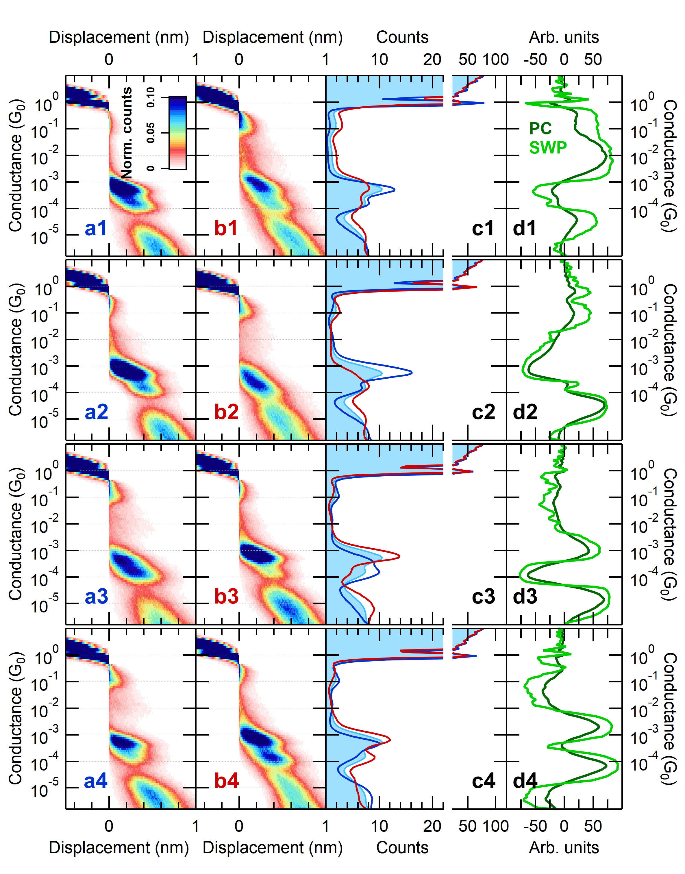
Figure 2: PCP-NN analysis of Au-BPY-Au single-molecule junctions according to the four leading principal components. The analysis according to $P^{(n)}$ is presented in the $n$th row, the corresponding principal components are shown by dark green lines in panels (d1-d4). The PCP-NN method classifies all the traces to two groups, trace class (a) and (b). The corresponding 2D histograms are respectively shown in panels (a1-a4) and (b1-b4), whereas the 1D histograms are shown in panels (c1-c4) by blue lines (trace class (a)) and by red lines (trace class (b)). As a reference, the blue area graphs represent the 1D histogram for the whole dataset. In panels (d1-d4) the light green lines represent the corresponding summed-weight-product of the neural network. The entire dataset includes 18301 traces, from which all the traces are classified into one or the other trace class. For the various principal components, the number of traces in a trace class varies in the range of $48.5\%-51.5\%$ of all traces.

First of all, it is clear from Figs. 2d1-d4 that the SWPs very much resemble the principal components for all the PCs. In the case of panels d2 and d3, the shape of the PC and the SWP is almost identical, whereas, in case of panels d1 and d4, the SWP refines and enhances the features of the PC, i.e. significantly sharper transitions are observed between the negative and positive regions. This already underpins the added value of the neural network extension of the simple PCP analysis: whereas the NN analysis basically learns the internal correlations of the dataset from the PCP, it is able to define more precise and sharper boundaries between the relevant conductance regions. Furthermore, we emphasize again that in the case of the simple PCP method, the best threshold PCP value between the two trace classes is ill-defined (it is not generally zero), but the NN extension is able to find the optimal boundary between the two trace classes.

The analysis according to the first principal component enhances/suppresses both histogram peaks in the molecular region compared to the entire dataset. The background counts outside of the region of the molecular peaks behave vice versa, these are strongly suppressed/enhanced for the trace class (a)/(b) (see the blue and red lines in Fig. 2c1, and the corresponding 2D histograms in Fig. 2a1/a2, where the blue/red label color matches the linecolor of the subset histograms in panel c1). Interestingly, the weight in the single-atom ($1\,$G₀) region and a bit higher conductance ($\approx 1.2-1.5\,$G₀) is also a significant part of the data filtering. For trace class (a)/(b) the $1\,$G₀ peak is significantly enhanced/suppressed, whereas the weight at somewhat higher conductance is suppressed/enhanced, respectively. The latter phenomenon resembles the precursor effect reported in Ag-CO-Ag single-molecule junctions,³³ where the presence of the parallel-bound CO molecule spoils the formation of the clear $1\,$G₀ single-atom configuration, and rather a broader weight is observed at somewhat larger conductance. Here, we argue, that well-defined BPY single-molecule junctions are best formed after the rupture of a well-defined single-atom Au junction with $1\,$G₀ conductance. Any contamination, that spoils the formation of this clean single-atom structure also hinders the formation of a well-defined Au-BPY-Au single-molecule structure, but rather enhances the background weight above the single-molecule and single-atom conductance. Therefore, the PCP-NN analysis according to the first principal component is efficient in separating ideal molecular traces with well-defined Au-BPY-Au single-molecule configurations from obscured molecular traces. The PCP-NN analysis also highlights precursors of these trace classes in the $1\,$G₀ conductance region.

While $P^{(1)}$ filters the traces by suppressing or highlighting both molecular peaks, the further principal components perform a peak-specific classification. In case of $P^{(2)}$, the HighG molecular peak is either enhanced or suppressed and the LowG molecular peak is left unchanged (Fig. 2a2-c2); in case of $P^{(3)}$, either the HighG peak is enhanced and the LowG peak is suppressed, or vica versa (Fig. 2a3-c3); in case of $P^{(4)}$, the LowG peak is enhanced or suppressed, whereas the HighG peak is left more-or-less unchanged (Fig. 2a4-c4). Although the PCP-NN analysis does not uncover the physical origin of these various trace classes, it makes it very clear, that the average and well-known junction evolution seen on the 2D conductance histogram of the BPY molecules (Fig. 1a) is definitely not a single representative junction evolution. While the former (Fig. 1a) implies the sequential formation of the HighG and LowG configurations on the same trace, the PCP-NN-based data sorting very clearly highlights the presence of various fundamentally different junction evolution trajectories, which all represent a significant portion of the traces. More importantly, these possible significant junction evolution trajectories are not sorted according to some subjective manual data filtering criterion, nor by a black-box-like high-complexity machine learning method, rather they rely on the well-defined internal correlations of the dataset.

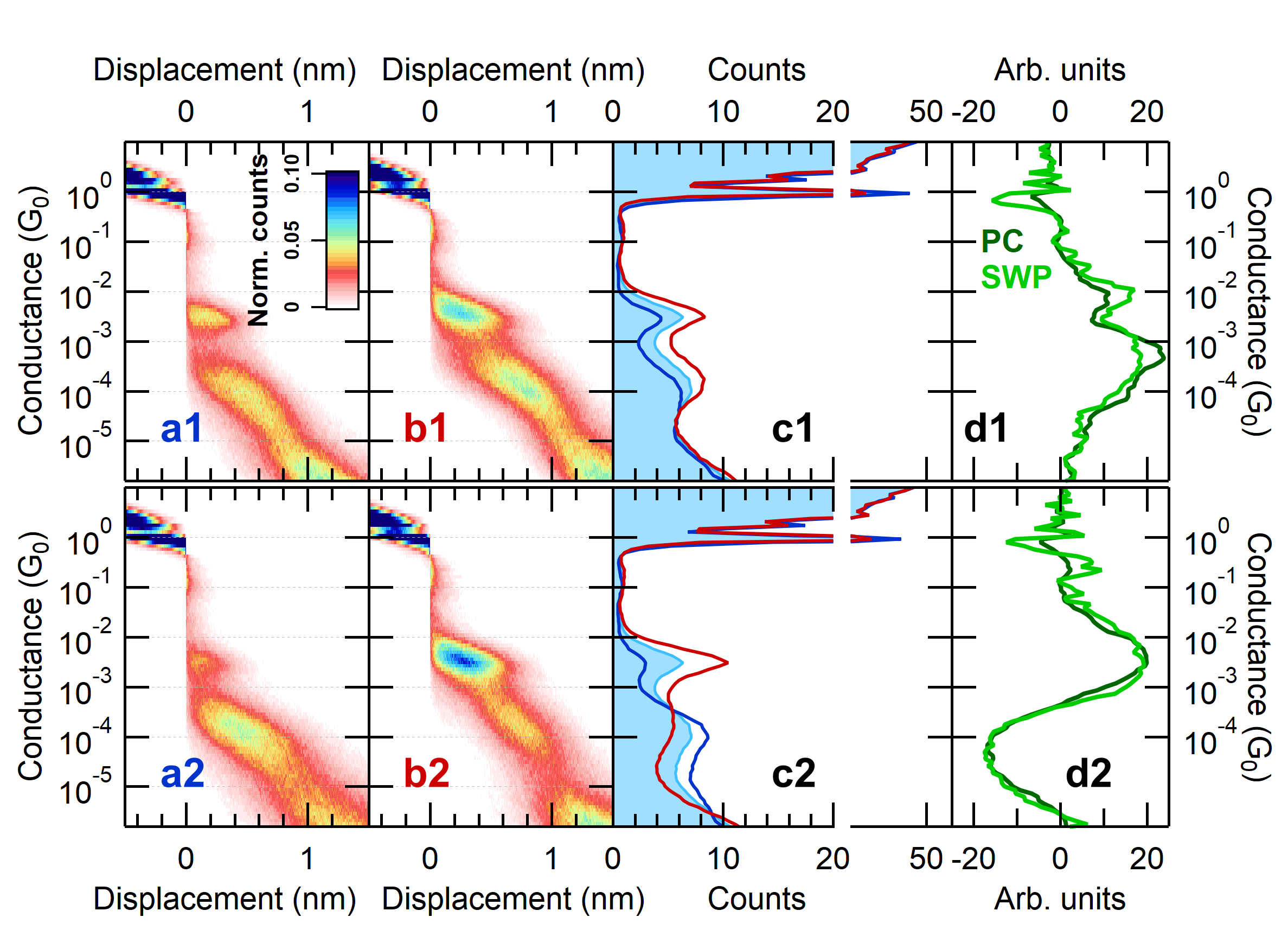
Figure 3: PCP-NN analysis of Au-DAF-Au single-molecule junctions. The analysis according to $P^{(1)}$ and $P^{(2)}$ is respectively presented in the first and second row, the corresponding principal components are shown by dark green lines in panels (d1,d2). Panels (a1,a2) and (b1,b2) respectively demonstrate the 2D histograms of trace classes (a) and (b). The corresponding 1D histograms are respectively shown by blue and red lines in panels (c1,c2) in comparison to the histogram of the entire dataset (light blue area graph). In panels (d1,d2) the light green lines represent the corresponding summed-weight-product of the neural network. The entire dataset includes 7001 traces. The selected trace classes include $45\%-55\%$ of all traces.

Next, we perform a similar analysis on Au-DAF-Au single-molecule junctions (Fig. 3). The analysis according to $P^{(1)}$ (Fig. 3a1-d1) provides a somewhat similar result to the BPY molecules: trace class (a) yields the suppression of both molecular peaks, whereas trace class (b) enhances both molecular peaks. The effect of the projection to $P^{(2)}$ (Fig. 3a2-d2) is similar to the $P^{(3)}$ projection in case of the BPY molecules, i.e. in trace class (a) the HighG peak is suppressed, and the LowG peak is enhanced, and vice versa in trace class (b). In case of DAF molecules, the further principal component projections ($P^{(3)}$ and $P^{(4)}$) show very similar results to the $P^{(2)}$ projection.

To demonstrate the robustness of the PCP-NN analysis, we have also investigated its sensitivity on the preparation of the data. First, we have found that independent measurements on Au-BPY-Au junctions using two completely different measurement methods (MCBJ/STM break junctions) yield very similar results, underpinning that the correlation plot and its principal components indeed act as specific fingerprints of the possible single-molecule junction evolution trajectories. On the other hand, the PCP-NN method is found to be especially sensitive to the temporal homogeneity of the data, inhomogeneous data portions may introduce severe artifacts to the analysis. These aspects are discussed in more detail in the ESI.

EPCP-aided interpretation of single-molecule $1/f$-type noise measurements. As mentioned in the introduction, the scaling of the $1/f$-type noise amplitude with the junction conductance supplies fundamental information about the nature of the metal-molecule bonds.^{14, 11, 18, 12, 21} Here, we investigate the noise characteristics of the widely-studied Au-BPY-Au single-molecule junctions. As an initial hypothesis, in the HighG configuration the aromatic ring also couples to the metallic apex which may introduce a significant through-space contribution to the transport, whereas the LowG configuration relies on the transport through the linkers, anticipating through-bond characteristics. The measured noise characteristics, i.e. the most probable relative conductance noise, $\Delta G/G$ is shown by black line in Fig. 4a for the entire dataset (see the light blue area graph in Fig. 4c for the corresponding conductance histogram in the molecular region, and the ESI for more details on the noise analysis). This curve indeed exhibits through-space-type $\Delta G/G\sim\mathrm{const.}$ characteristics at the top tail of the HighG peak, and through-bond-type $\Delta G/G\sim G^{-0.5}$ characteristics at the bottom tail of the LowG peak. As a comparison, the orange dashed line represents the envisioned noise evolution according to the above discussed considerations, i.e. through-space-type noise in the entire HighG region and through-bond-type noise in the entire LowG region. More precisely, the orange dashed line extrapolates the best fitting $\Delta G/G\sim G^{-0.5}$ / $\Delta G/G\sim\mathrm{const.}$ tendencies at the low/high conductance sides of the investigated conductance region to the entire conductance range assuming a sharp transition at the intersection of these lines. It is clear that in the intermediate conductance region the noise data clearly deviate from this supposed behavior. This intermediate conductance region, however, is positioned around the conductance boundary between the HighG and LowG configurations ($G\approx 4\cdot 10^{-3}\,$G₀), where the largest diversity of the possible junction evolution paths appears according to the above PCP analysis. Therefore, the interpretation of the unexpected noise evolution would remain highly speculative as long as the noise contributions of the two molecular configurations are not separated very clearly.

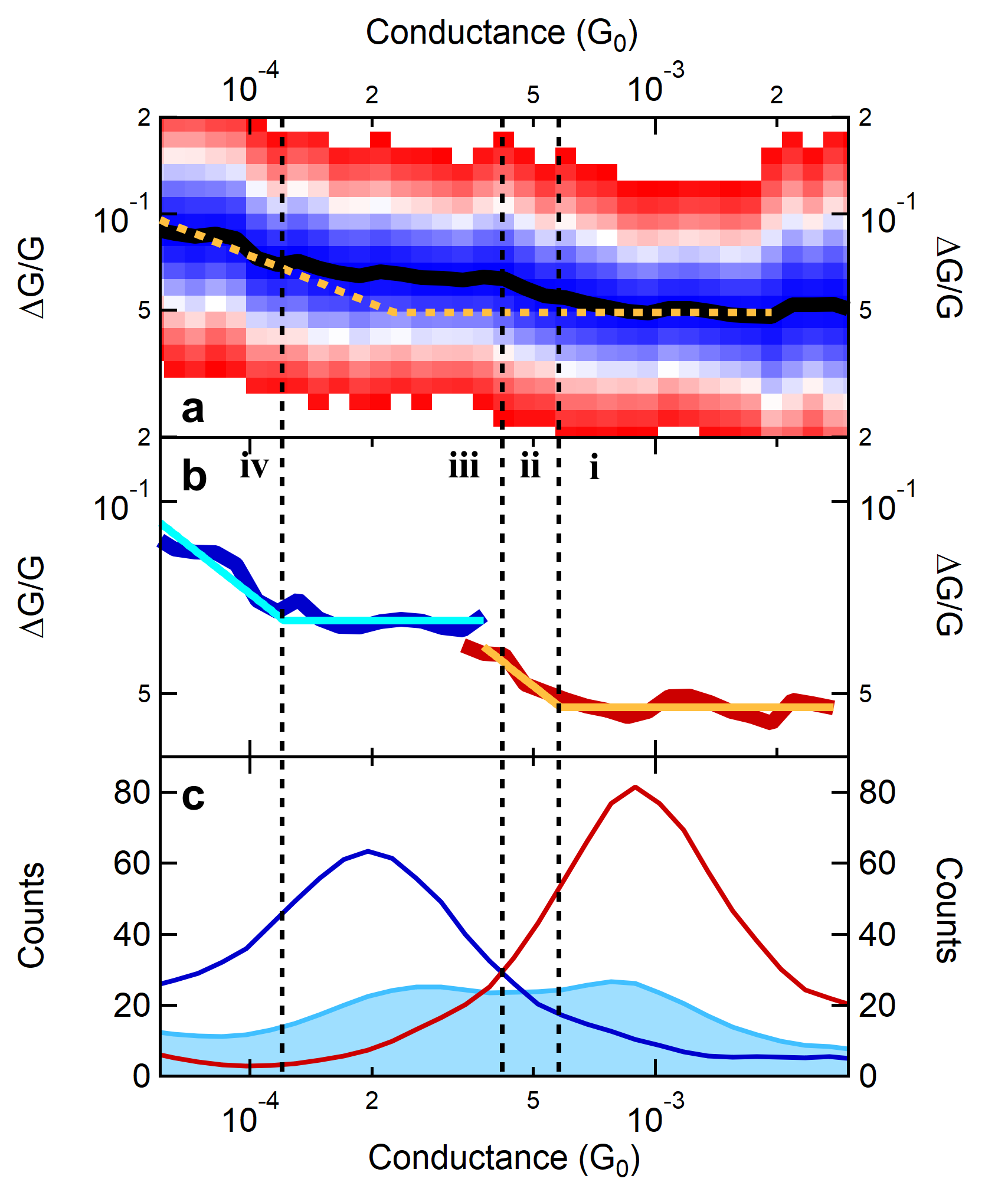
Figure 4: Configuration-specific $1/f$-type noise analysis of Au-BPY-Au junctions. (a) Most probable relative conductance noise as a function of the conductance (black line) for the entire dataset. The colorscale illustrates the scattering of the noise data (see ESI for more details). The orange dashed line represents the hypothetical noise evolution discussed in the text. (b) Configuration-specific noise analysis demonstrating the noise evolution separately for the HighG (red) and LowG (blue) configurations. The orange and light blue lines represent the best-fitting model curves. (c) Conductance histogram of the entire dataset (light blue area graph) together with the configuration-specific EPCP projections (blue and red lines). The roman numbers together with the black dashed boundary lines illustrate the four characteristic regions of the junction evolution, as discussed in the text.

The EPCP-based selection demonstrated by the red and blue histograms in Fig. 1b offers a unique possibility to very clearly separate the HighG and LowG configurations, investigating their noise characteristics separately. The most probable $\Delta G/G$ values can be generated separately for these two data subsets, as demonstrated by the red and blue curves in Fig. 4b. According to our hypothesis, we would expect $\Delta G/G\sim\mathrm{const.}$ for the HighG subset (red) and $\Delta G/G\sim G^{-0.5}$ for the LowG subset (blue). This is, however, clearly contradicted by the data. Instead of the markedly different noise characteristics of the HighG and the LowG configurations, both configurations exhibit very similar noise evolution with through-space-type constant $\Delta G/G$ at the top part of the actual subset histogram peak, and through-bond-type characteristics ($\Delta G/G\sim G^{-0.5}$) at the bottom tail of the subset histogram peaks. The latter tendencies are also illustrated in Fig. 4b by the orange (light blue) line representing the best fitting model curves assuming constant/$G^{-0.5}$ noise evolution above/below a certain conductance threshold for HighG (LowG) configurations. Again, the deviation from the expected behavior is the most striking in the intermediate conductance region, where both the HighG and the LowG data subsets exhibit opposite behavior to the initial hypothesis, i.e. through-bond-type behavior for the HighG configuration and through-space-type behavior for the LowG configuration.

According to this configuration-specific analysis, we can identify four distinct conductance intervals according to distinct noise evolution characteristics (see the roman numbers in panel Fig. 4b and the separating dashed lines). (i) At the top part of the HighG peak the HighG configuration indeed exhibits additional $\pi$-coupling between the pyridine ring and the electrodes, giving rise to constant through-space-like noise characteristics. (ii) As the HighG configuration is stretched (i.e. at the bottom tail of the HighG peak) this coupling vanishes giving rise to increasing, through-bond-type noise characteristics. (iii) At the top part of the LowG peak again a significant constant, through-space noise contribution is observed, indicating that the pyridine ring couples to the side of the electrode in this region as well. (iv) Finally, as the LowG configuration is stretched, this $\pi$-coupling vanishes again, the molecule straightens out, and again increasing, through-bond-type noise characteristics are observed (bottom tail of the LowG peak). More precisely, the borders between the i/ii and iii/iv intervals are identified by the points, where the fitted noise characteristics (orange and light blue lines in panel (b)) turn from constant to $\Delta G/G\sim G^{-0.5}$ dependency ($G=5.8\cdot 10^{-4}\,$G₀ for i/ii and $G=1.2\cdot 10^{-4}\,$G₀ for ii/iv), whereas the border between the ii/iii intervals is the crossing point of the HighG and LowG histograms in panel (c), $G=4.2\cdot 10^{-4}\,$G₀. Note, howevever, that these conductance regions rely on a rather simplifyed model, considering exactly $\sim G^{-0.5}$ and $\sim G^{0}$ scaling exponents with a sharp transition between these. It would be more realistic to permit deviations from these limiting scaling factors, and a more gradual transition between the two distinct behaviors, but due to the limitied resolution of the noise data we rather apply the most simple model grabbing the most important rough tendencies.

The above, peak-specific insight to the noise characteristics explores the cases, where solely the HighG or solely the LowG configurations appear. However, the noise evolution of the entire dataset (black curve in Fig. 4a) , where the two molecular configurations often appear sequentially on the same trace, follows the same trends as the separated configurations (through-space/through-bond/through-space/through-bond characteristics in regions i/ii/iii/iv, respectively). This suggests, that the above-described physical mechanisms are not specific to the separate, or the sequential appearance of the two configurations, rather a specific conductance interval (i-iv) always shows similar noise evolution. In case of the sequential appearance of the two configurations, we argue that around the ii/iii boundary, the molecule may jump to another bonding site, such that the pyridine ring again flips to the side of the electrode giving rise to a significant constant, through-space noise contribution.

3 Conclusions

In conclusion, we have demonstrated the merits of PCP-based unsupervised data classification in single-molecule break junction measurements. According to our analysis on room-temperature Au-BPY-Au and Au-DAF-Au single-molecule structures, all the leading principal components project the conductance traces to highly relevant data subsets, signaling alternative junction evolution trajectories which are obscured on the 1D and 2D conductance histograms. These results demonstrate an efficient classification according to the well-established and well-visualized internal correlations of the dataset, i.e. the PCP-method lacks the disadvantage of the black-box-like nature of more complex machine learning approaches, as well as the subjective nature of custom-created manual data filtering algorithms.

Finally, we demonstrated that these efficient data classification capabilities can be exploited in the measurement of further physical quantities, where the mixture of alternative junction evolution trajectories would obscure the analysis. In particular, the PCP-method enabled us to perform a configuration-specific 1/f-type noise analysis, uncovering refined details of the junction evolution: we identified the coupling of the aromatic ring to the electrodes through the $\pi$ orbitals in two distinct conductance regions, and its subsequent uncoupling as these configurations are stretched.

Author contributions

The measurements were performed by G. Mezei and Z. Balogh (combined noise and conductance measurements) and by A. Magyarkuti and N. Tenk (traditional conductance measurements). The PCP analysis was performed by Z. Balogh, N. Tenk and G. Mezei, the neural network supplement was implemented by N. Tenk and A. Magyarkuti. The noise analysis was performed by G. Mezei and Z. Balogh. The idea of the project was conceived and the project was supervised by A. Halbritter, with a fundamental contribution of Z. Balogh in the noise measurement part. The manuscript was written by A. Halbritter and Z. Balogh with remarks from all authors.

References

- Cuevas and Scheer 2010 J. C. Cuevas and E. Scheer, Molecular Electronics: An Introduction to Theory and Experiment, World Scientific, 2010.
- Aradhya and Venkataraman 2013 S. V. Aradhya and L. Venkataraman, Nature Nanotechnology, 2013, 8, 399–410.
- Xin et al. 2019 N. Xin, J. Guan, C. Zhou, X. Chen, C. Gu, Y. Li, M. A. Ratner, A. Nitzan, J. F. Stoddart and X. Guo, Nature Reviews Physics, 2019, 1, 211–230.
- Gehring et al. 2019 P. Gehring, J. M. Thijssen and H. S. J. van der Zant, Nature Reviews Physics, 2019, 1, 381–396.
- Evers et al. 2020 F. Evers, R. Korytár, S. Tewari and J. M. van Ruitenbeek, Rev. Mod. Phys., 2020, 92, 035001.
- Muller et al. 1992 C. J. Muller, J. M. van Ruitenbeek and L. J. de Jongh, Physica C Superconductivity, 1992, 191, 485–504.
- Xu and Tao 2003 B. Xu and N. J. Tao, Science, 2003, 301, 1221–1223.
- Frei et al. 2011 M. Frei, S. V. Aradhya, M. Koentopp, M. S. Hybertsen and L. Venkataraman, Nano Letters, 2011, 11, 1518–1523.
- Nef et al. 2012 C. Nef, P. L. T. M. Frederix, J. Brunner, C. Schönenberger and M. Calame, Nanotechnology, 2012, 23, 365201.
- Mohos et al. 2014 M. Mohos, I. V. Pobelov, V. Kolivoška, G. Mészáros, P. Broekmann and T. Wandlowski, The Journal of Physical Chemistry Letters, 2014, 5, 3560–3564.
- Magyarkuti et al. 2018 A. Magyarkuti, O. Adak, A. Halbritter and L. Venkataraman, Nanoscale, 2018, 10, 3362–3368.
- Balogh et al. 2021 Z. Balogh, G. Mezei, L. Pósa, B. Sánta, A. Magyarkuti and A. Halbritter, Nano Futures, 2021, 5, 042002.
- Djukic and van Ruitenbeek 2006 D. Djukic and J. M. van Ruitenbeek, Nano Letters, 2006, 6, 789–793.
- Adak et al. 2015 O. Adak, E. Rosenthal, J. Meisner, E. F. Andrade, A. N. Pasupathy, C. Nuckolls, M. S. Hybertsen and L. Venkataraman, Nano Letters, 2015, 15, 4143–4149.
- Karimi et al. 2016 M. A. Karimi, S. G. Bahoosh, M. Herz, R. Hayakawa, F. Pauly and E. Scheer, Nano Letters, 2016, 16, 1803–1807.
- Lumbroso et al. 2018 O. S. Lumbroso, L. Simine, A. Nitzan, D. Segal and O. Tal, Nature, 2018, 562, 240–244.
- Tang et al. 2019 C. Tang, L. Chen, L. Zhang, Z. Chen, G. Li, Z. Yan, L. Lin, J. Liu, L. Huang, Y. Ye, Y. Hua, J. Shi, H. Xia and W. Hong, Angewandte Chemie International Edition, 2019, 58, 10601–10605.
- Wu et al. 2020 C. Wu, D. Bates, S. Sangtarash, N. Ferri, A. Thomas, S. J. Higgins, C. M. Robertson, R. J. Nichols, H. Sadeghi and A. Vezzoli, Nano Letters, 2020, 20, 7980–7986.
- Yuan et al. 2021 S. Yuan, T. Gao, W. Cao, Z. Pan, J. Liu, J. Shi and W. Hong, Small Methods, 2021, 5, 2001064.
- Kim and Song 2021 Y. Kim and H. Song, Applied Physics Reviews, 2021, 8, 011303.
- Pan et al. 2022 Z. Pan, L. Chen, C. Tang, Y. Hu, S. Yuan, T. Gao, J. Shi, J. Shi, Y. Yang and W. Hong, Small, 2022, 18, 2107220.
- Shein-Lumbroso et al. 2022 O. Shein-Lumbroso, J. Liu, A. Shastry, D. Segal and O. Tal, Phys. Rev. Lett., 2022, 128, 237701.
- Widawsky et al. 2012 J. R. Widawsky, P. Darancet, J. B. Neaton and L. Venkataraman, Nano Letters, 2012, 12, 354–358.
- Rincón-García et al. 2016 L. Rincón-García, C. Evangeli, G. Rubio-Bollinger and N. Agraït, Chem. Soc. Rev., 2016, 45, 4285–4306.
- Cui et al. 2017 L. Cui, W. Jeong, S. Hur, M. Matt, J. C. Klöckner, F. Pauly, P. Nielaba, J. C. Cuevas, E. Meyhofer and P. Reddy, Science, 2017, 355, 1192–1195.
- Cui et al. 2019 L. Cui, S. Hur, Z. A. Akbar, J. C. Klöckner, W. Jeong, F. Pauly, S.-Y. Jang, P. Reddy and E. Meyhofer, Nature, 2019, 572, 628–633.
- Mosso et al. 2019 N. Mosso, H. Sadeghi, A. Gemma, S. Sangtarash, U. Drechsler, C. Lambert and B. Gotsmann, Nano Letters, 2019, 19, 7614–7622.
- Smit et al. 2002 R. H. M. Smit, Y. Noat, C. Untiedt, N. D. Lang, M. C. van Hemert and J. M. van Ruitenbeek, Nature, 2002, 419, 906–909.
- Csonka et al. 2004 S. Csonka, A. Halbritter, G. Mihály, O. I. Shklyarevskii, S. Speller and H. van Kempen, Phys. Rev. Lett., 2004, 93, 016802.
- Scheer et al. 1998 E. Scheer, N. Agraït, J. C. Cuevas, A. L. Yeyati, B. Ludoph, A. Martín-Rodero, G. R. Bollinger, J. M. van Ruitenbeek and C. Urbina, Nature, 1998, 394, 154–157.
- Makk et al. 2008 P. Makk, S. Csonka and A. Halbritter, Phys. Rev. B, 2008, 78, 045414.
- Makk et al. 2012 P. Makk, Z. Balogh, S. Csonka and A. Halbritter, Nanoscale, 2012, 4, 4739–4745.
- Balogh et al. 2014 Z. Balogh, D. Visontai, P. Makk, K. Gillemot, L. Oroszlány, L. Pósa, C. Lambert and A. Halbritter, Nanoscale, 2014, 6, 14784–14791.
- Inkpen et al. 2015 M. S. Inkpen, M. Lemmer, N. Fitzpatrick, D. C. Milan, R. J. Nichols, N. J. Long and T. Albrecht, Journal of the American Chemical Society, 2015, 137, 9971–9981.
- Huang et al. 2017 C. Huang, M. Jevric, A. Borges, S. T. Olsen, J. M. Hamill, J.-T. Zheng, Y. Yang, A. Rudnev, M. Baghernejad, P. Broekmann, A. U. Petersen, T. Wandlowski, K. V. Mikkelsen, G. C. Solomon, M. Brøndsted Nielsen and W. Hong, Nature Communications, 2017, 8, 15436.
- Bro-Jørgensen et al. 2022 W. Bro-Jørgensen, J. M. Hamill, R. Bro and G. C. Solomon, Chem. Soc. Rev., 2022, 51, 6875–6892.
- Lemmer et al. 2016 M. Lemmer, M. S. Inkpen, K. Kornysheva, N. J. Long and T. Albrecht, Nature Communications, 2016, 7, 12922.
- Wu et al. 2017 B. H. Wu, J. A. Ivie, T. K. Johnson and O. L. A. Monti, The Journal of Chemical Physics, 2017, 146, 092321.
- Lauritzen et al. 2018 K. P. Lauritzen, A. Magyarkuti, Z. Balogh, A. Halbritter and G. C. Solomon, The Journal of Chemical Physics, 2018, 148, 084111.
- Cabosart et al. 2019 D. Cabosart, M. El Abbassi, D. Stefani, R. Frisenda, M. Calame, H. S. J. van der Zant and M. L. Perrin, Applied Physics Letters, 2019, 114, 143102.
- Bamberger et al. 2020 N. D. Bamberger, J. A. Ivie, K. N. Parida, D. V. McGrath and O. L. A. Monti, The Journal of Physical Chemistry C, 2020, 124, 18302–18315.
- Huang et al. 2020 F. Huang, R. Li, G. Wang, J. Zheng, Y. Tang, J. Liu, Y. Yang, Y. Yao, J. Shi and W. Hong, Phys. Chem. Chem. Phys., 2020, 22, 1674–1681.
- Fu et al. 2020 T. Fu, Y. Zang, Q. Zou, C. Nuckolls and L. Venkataraman, Nano Letters, 2020, 20, 3320–3325.
- Fu et al. 2021 T. Fu, K. Frommer, C. Nuckolls and L. Venkataraman, The Journal of Physical Chemistry Letters, 2021, 12, 10802–10807.
- Magyarkuti et al. 2021 A. Magyarkuti, Z. Balogh, G. Mezei and A. Halbritter, The Journal of Physical Chemistry Letters, 2021, 12, 1759–1764.
- Vladyka and Albrecht 2020 A. Vladyka and T. Albrecht, Machine Learning: Science and Technology, 2020, 1, 035013.
- Halbritter et al. 2010 A. Halbritter, P. Makk, S. MacKowiak, S. Csonka, M. Wawrzyniak and J. Martinek, Physical Review Letters, 2010, 105, 1–4.
- Makk et al. 2012 P. Makk, D. Tomaszewski, J. Martinek, Z. Balogh, S. Csonka, M. Wawrzyniak, M. Frei, L. Venkataraman and A. Halbritter, ACS Nano, 2012, 6, 3411–3423.
- Aradhya et al. 2013 S. V. Aradhya, M. Frei, A. Halbritter and L. Venkataraman, ACS Nano, 2013, 7, 3706–3712.
- Magyarkuti et al. 2017 A. Magyarkuti, K. P. Lauritzen, Z. Balogh, A. Nyáry, G. Mészáros, P. Makk, G. C. Solomon and A. Halbritter, The Journal of Chemical Physics, 2017, 146, 092319.
- Hamill et al. 2018 J. M. Hamill, X. T. Zhao, G. Mészáros, M. R. Bryce and M. Arenz, Phys. Rev. Lett., 2018, 120, 016601.
- Magyarkuti et al. 2020 A. Magyarkuti, N. Balogh, Z. Balogh, L. Venkataraman and A. Halbritter, Nanoscale, 2020, 12, 8355–8363.
- Quek et al. 2009 S. Y. Quek, M. Kamenetska, M. L. Steigerwald, H. J. Choi, S. G. Louie, M. S. Hybertsen, J. B. Neaton and L. Venkataraman, Nature Nanotechnology, 2009, 4, 230–234.
- Kamenetska et al. 2010 M. Kamenetska, S. Y. Quek, A. C. Whalley, M. L. Steigerwald, H. J. Choi, S. G. Louie, C. Nuckolls, M. S. Hybertsen, J. B. Neaton and L. Venkataraman, Journal of the American Chemical Society, 2010, 132, 6817–6821.
- Aradhya et al. 2012 S. V. Aradhya, M. Frei, M. S. Hybertsen and L. Venkataraman, Nature Materials, 2012, 11, 872–876.
- Baghernejad et al. 2014 M. Baghernejad, D. Z. Manrique, C. Li, T. Pope, U. Zhumaev, I. Pobelov, P. Moreno-García, V. Kaliginedi, C. Huang, W. Hong, C. Lambert and T. Wandlowski, Chem. Commun., 2014, 50, 15975–15978.
- Isshiki et al. 2018 Y. Isshiki, S. Fujii, T. Nishino and M. Kiguchi, Physical Chemistry Chemical Physics, 2018, 20, 7947–7952.
- Mezei et al. 2020 G. Mezei, Z. Balogh, A. Magyarkuti and A. Halbritter, The Journal of Physical Chemistry Letters, 2020, 11, 8053–8059.
- Martin et al. 2008 C. A. Martin, D. Ding, J. K. Sørensen, T. Bjørnholm, J. M. Van Ruitenbeek and H. S. Van Der Zant, Journal of the American Chemical Society, 2008, 130, 13198–13199.
- Kim et al. 2014 T. Kim, P. Darancet, J. R. Widawsky, M. Kotiuga, S. Y. Quek, J. B. Neaton and L. Venkataraman, Nano Letters, 2014, 14, 794–798.