Direct comparison or indirect comparison via a series of counterfactual decompositions?

Abstract: We illustrate the point with an empirical analysis of assortative mating in the US, namely, that the outcome of comparing two distant groups can be sensitive to whether comparing the groups directly, or indirectly via a series of counterfactual decompositions involving the groups’ comparisons to some intermediate groups. We argue that the latter approach is typically more fit for its purpose.

Keywords: Age-discrimination; Assortative mating; Counterfactual decomposition; Naszodi–Mendonca method.
JEL classification: J12, C02.

1 Introduction

Counterfactual decompositions are commonly applied with the aim of quantifying differences between two groups. For instance, the aim can be to measure the degree of labour-market discrimination of an age-group (or a gender-group, or a religious-group) relative to another age-group (or another gender-group, or another religious-group) (see Oaxaca 1973). Another example is about quantifying the relative degree of marital sorting in different generations (see Naszodi  Mendonca 2019, Naszodi  Mendonca 20211).

There are certain applications, where the direct comparison of the two groups studied has no alternative as there is no intermediate group between them. E.g. there is no group between the polytheists and the monotheists that could allow us to take into account the differences between these two religious-groups gradually.

However, there are empirical applications of counterfactual decompositions, where a series of comparisons can serve as an alternative to the direct comparison. For instance, the young–old comparison on the labour-market can be conducted by comparing the young workers to the intermediate group of middle-aged workers, while also comparing the middle-aged workers to the old workers rather than comparing the two extreme age-groups directly.

Similarly, the marital sorting of non-consecutive generations can be compared not only directly. Those who were young adults in 1960 can be compared with those who were young adults 55 years later via the comparisons of some consecutive generations.

In this note, we make the point that the decompositions with a series of comparisons are typically more fit for the purpose of controlling for certain effects than the decompositions with direct comparison. This point is not new in labour economics. For instance, Richardson . (2013) study age-discrimination by a series of comparisons of fictitious applicants’ success rates where each pair of profiles to be compared are the same along a number of traits, while differ in terms of age by a few years. Thereby, they control for the effect of work experience inter alia without having to construct the counterfactuals of old workers with no work experience and young workers with 40 years of experience.

However, it is a novel point for the literature on assortative mating. Even recently, changes in the degree of sorting were commonly studied via the direct comparison of some observations distant in time. For instance, Eika . (2019) in their empirical study analyzing the assortative mating–household inequality nexus compare directly how American men and women were matched along the educational dimension in the years 1962 and 2013. Moreover, those papers on assortative mating that conduct a series of comparisons of consecutive generations, such as Permanyer . (2019), Naszodi  Mendonca (20211), do not highlight the significance of their choice. This gap is filled by our note.

Let us see what confounding factor has to be controlled for in the context of educational assortative mating. Quantifying the degree of sorting is possible through its effect on a directly observed variable, the share of educationally homogmaous couples. Changes in this share from one generation to another generation depends not only on the changes in the degree of sorting, but also on the changes in the structural availability of potential partners with various education levels. So, the factor to be controlled for is the pair of educational distributions of marriageable men and women.

Similarly to the work experience and the age of job applicants, the degree of sorting and the structural availability may not be independent of each other. For this reason, it can be difficult to construct a counterfactual generation where the marital sorting is the same as it was in a certain year (e.g. 1960), while the structural availability is the same as it was in a distant year (e.g. 2015). This difficulty is of the same source as the mental limitation preventing us to imagine a 60-years old and a 20-years old job applicant with same work experience.

However, it is relatively easy to construct the joint educational distributions of couples under various counterfactuals, where marital sorting and availability are measured within a reasonably short time period, e.g., a decade. These counterfactual distributions allow researchers to compare even very distant generations via a series of comparisons.

In the empirical part of this paper, we apply both the direct comparison and the series of comparisons to the degree of sorting of the early Silent Generation and the early Millennials. This example illustrates that the choice is not innocuous.

2 Data and method

We use census data on the joint educational distributions of both married and cohabiting heterosexual American couples. We refer to both types of unions as marriages. Similarly, we distinguish neither between husbands and male partners, nor between wives and female partners.

The data are from the Integrated Public Use Microdata Series (IPUMS). The observations are from the years 1960, 1970, 1980, 1990, 2000, 2010 and 2015. Following Eika . (2019), we work with four education levels: no high school degree, high school degree, some college, tertiary level diploma.

In the first empirical exercise, we work with data from 1960 and 2015 covering couples where the wives are between 28 and 57 years old. In the second exercise, we enrich the data with observations from 1990. In the third exercise, we use data from all the five intermediate decennial censuses while we restrict our analysis to marriages where the wives are between 26 and 35. Finally, we restrict the data to marriages with wives between 28 and 32 for analyzing the period of 2010–2015. Due to these restrictions, no couple is observed twice in any of the exercises. Therefore, the outcome of neither of our comparisons is effected by changes in sorting over the course of individuals’ lives.

We apply the NM-method developed by Naszodi  Mendonca (2019) and Naszodi  Mendonca (20211) for constructing the counterfactual joint distributions. This choice is motivated by the validation exercise of Naszodi  Mendonca (20211): they show that while the outcomes of certain decompositions obtained with the NM are in accord with survey evidence on Americans’ self-reported marital preferences, this is not the case with certain alternative methods.

3 Empirical results

Figure 1 presents the outcomes of the decompositions. Its dashed black line shows the result of a direct comparison: in 1960, 58.8% of the observed couples with wives between 28 and 57 were homogamous. This share would have been decreased by 3 percentage points by 2015 provided the education levels of young adults remained the same as in 1960. If we also use the intermediate observation from 1990, then the same effect is quantified to be higher in absolute terms (-4.7=54.1-58.8, see the gray dotted line).

If we use all the intermediate observations from the census, while we also change the age group analyzed then the effect studied is found to be even higher in absolute terms     (-5.5=49-54.5 percentage points, see the black continuous line). To see whether the difference is due to the shrinking age brackets, we follow Eika . (2019) and perform an alternative set of decompositions. In this exercise, we work with the [26,35] age category and keep the structural availability fixed at the base year of 1960, while we allow the degree of marital sorting to vary over time. This alternative direct comparison-based decomposition assigns a change of the same magnitude (-3.1=51.4-54.5) to the changing sorting between 1960 and 2015 as the first direct comparison-based decomposition (see the dashed gray line).

All in all, the changes in sorting are quantified to have contributed much more to the change in the share of educationally homogamous couples between 1960 and 2015, if their effects are measured by a series of comparisons of consecutive generations rather than by a direct comparison of non-consecutive generations.

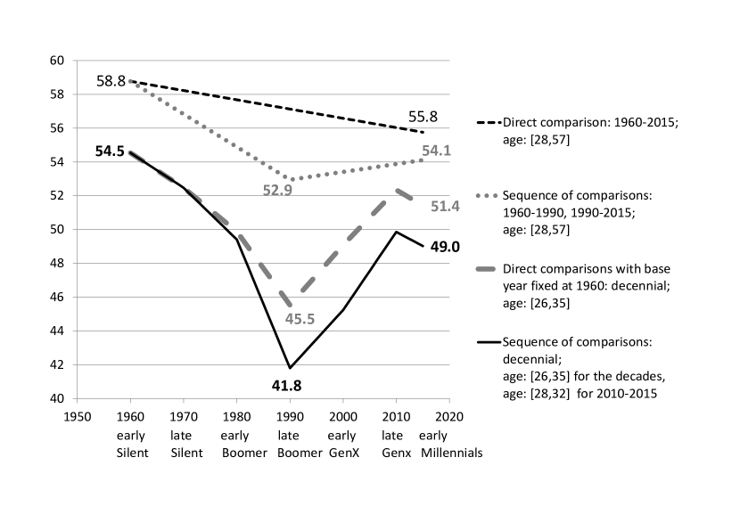
Figure 1: Counterfactual shares of educationally homogamous couples (in %) – counterfactuals are constructed by the NM

Source: author’s calculations using US census data from IPUMS about the education level of married couples and cohabiting couples.

4 Conclusion

Performing counterfactual decomposition with a sequence of comparisons allows us to compare observations of two groups distant in time or in any other dimension by using intermediate observations representing gradual transition from one of the groups to the other group studied. This note promoted the gradual approach.

We argued that this approach has the advantage relative to the direct comparison of being suitable for controlling for the effects of some confounding factors. Also, we illustrated with an empirical application that the outcome of the decomposition can be sensitive to the choice of the approach. Our example was taken from a strand of the empirical counterfactual decomposition literature where the opportunity of sequential comparison has not always been exploited.

Appendix A: Sensitivity analysis with respect to the method used for constructing the counterfactuals

In this appendix, we show that our point on the direct versus indirect comparison is robust to the choice of how the counterfactuals are constructed. In particular, we illustrate with the same empirical application presented in the main part of the paper that the outcome of the decomposition can be sensitive to the choice between the direct comparison and the sequential comparison even if the counterfactuals are constructed by the iterative proportional fitting (IPF) algorithm (rather than the NM).

The IPF algorithm, or as it is also commonly referred to, the RAS algorithm, is a mathematical scaling procedure which has been widely used by social scientists to standardize the marginal distribution of a contingency table to some fixed value, while retaining a specific association between the row and the column variables. The retained association is the similarity of these variables captured by the odds-ratio.

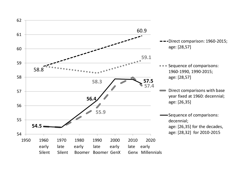
Figure 2: Counterfactual shares of educationally homogamous couples (in %) – counterfactuals are constructed by the IPF

Source: author’s calculations using US census data from IPUMS about the education level of married couples and cohabiting couples.

Figure 2 presents the outcomes of the corresponding decompositions. By comparing Figure 1 and Figure 2, it is apparent that the identified trend of sorting is highly sensitive to how the counterfactuals are constructed. By applying the NM, the degree of sorting along the educational displays a U-shaped trend (see the black, continuous line in Figure 1). As it is pointed out by Naszodi (2023), the U-pattern is consistent not only with the forming consensus in the income and wealth inequality literature about the historical trend of the monetary dimensions of inequality, but also with the survey evidence about Americans’ self-reported marital preferences.

By contrast, the IPF-based decomposition suggests that the degree of sorting was either increasing or stagnant over the analyzed decades (see the black, continuous line in Figure 2). This trend is similar to the trend identified by Eika . (2019) with their aggregate marital sorting indicator (see Figure 4 in Eika . 2019).

Despite the monotonous increase in sorting is not corroborated by the survey evidence from the Pew Research Center analyzed by Naszodi  Mendonca (20211), Naszodi (2023) and Naszodi (2022), the IPF has been a popular method for constructing counterfactuals until recently. Therefore, “old school” researchers may find it interesting to see whether the choice between the direct comparison and the sequence of comparisons makes a difference provided the counterfactuals can be constructed by the IPF.

Figure 2 shows that the choice matters. In 2015, the share of educationally homogamous couples would have been 2.1 (=60.9-58.8) percentage points higher among the couples with wives between 28 and 57 relative to 1960 under the direct comparison (see the dashed black line). Whereas the same effect is quantified to be much smaller (0.3=59.1-58.8 percentage points) if we also use the intermediate observation from 1990, but we change neither the age group studied, nor the method for constructing the counterfactuals (see the gray dotted line).

If we use all the intermediate observations from the five census years of 1970, 1980, 1990, 2000, 2010, and work with the [26,35] age category then the same effect is measured to be 3 (=57.5-54.5) percentage points (see the black continuous line). We obtain roughly the same effect (2.9 = 57.4-54.5) if we keep on working with the [26,35] age category, while fixing the structural availability at the base year of 1960 (see the dashed gray line).

All in all, we find that the magnitude of the effect studied can be sensitive to the choice between the series of comparisons of consecutive generations and the direct comparison of non-consecutive generations irrespective of the method used for constructing counterfactuals.

Appendix B: Counterfactual decomposition with the NM-method

This appendix offers a detailed explanation on how the empirical decompositions are performed with the NM-method. The NM-method is based on the scalar-valued sorting indicator proposed by Liu  Lu (2006) (henceforth LL-indicator) and the generalized, matrix-valued LL-indicator proposed by Naszodi  Mendonca (20211). First, we introduce the original LL-indicator and the generalized LL-indicator. Then, we present the NM-method. Finally, we introduce the decomposition scheme used.

The original LL-indicator

The LL-indicator, as it was originally developed by Liu  Lu (2006), is a scalar-valued, ordinal measure that can be applied if the assorted trait is a one-dimensional dichotomous variable (e.g. taking the values $L$ or $H$).

The original LL-indicator is identical to the value taken by a function ($f:\mathbb{N}^{2\times 2}\mapsto\mathbb{R}$) that assigns a scalar to a 2-by-2 contingency table, where the contingency table is of the form

$$Z^{2\text{-by-}2}=\begin{bmatrix}N_{L,L}&N_{L,H}\\ N_{H,L}&N_{H,H}\end{bmatrix}\;.$$ (1)

$N_{H,H}$ (/$N_{L,L}$) denotes the number of homogamous couples, where both spouses are $H$ (/$L$) type. $N_{L,H}$ (/$N_{H,L}$) stands for the number of heterogamous couples, where the husbands (/wives) are $L$-type, while the wives (/husbands) are $H$-type.

Furthermore, we introduce the notations $N_{H,\cdot}=N_{H,H}+N_{H,L}$, $N_{\cdot,H}=N_{L,H}+N_{H,H}$, $N_{\cdot,\cdot}=N_{\cdot,H}+N_{\cdot,L}$. For a given triad of $\{N_{H,\cdot},N_{\cdot,H},N_{\cdot,\cdot}\}$, $Q={N_{H,\cdot}N_{\cdot,H}}/{N_{\cdot,\cdot}}$ denotes the expected number of $H$,$H$-type couples under random matching. We define $Q^{-}$ as the biggest integer being smaller than, or equal to, $Q$.

It is important to note that any actual realization of the joint distribution $Z^{\text{act},{2\text{-by-}2}}\in\mathbb{N}^{2\times 2}$ with a given triad can be represented by any of its cells. For instance, the actual value of the ${H,H}$ cell, i.e., $N^{\text{act}}_{H,H}$, can represent $Z^{\text{act},{2\text{-by-}2}}$, because all the other three cells’ actual values are uniquely determined by the triad and $N^{\text{act}}_{H,H}$. Therefore, there is a unique ranking of the joint distributions with the same triad. This ranking is defined simply by the ranking of the ${H,H}$ cells: that table ranks higher which has higher value in its ${H,H}$ cell.

The original LL-indicator defines a ranking among the joint distributions with the same, but also with different, triads by ranking their values at the ${H,H}$ cell relative to all possible values of $N_{H,H}$ conditional on the triad. Under the assumption of non-negative sorting (i.e., $Q^{-}\leq N^{\text{act}}_{H,H}$), the original LL-measure is equivalent to the simplified LL-measure defined as:

$$\text{LL}^{\text{sim}}(Z^{\text{act},2\text{-by-}2})=\frac{N^{\text{act}}_{H,H}-\text{min}(N_{H,H}|N_{H,\cdot},N_{\cdot,H},N_{\cdot,\cdot})}{\text{max}(N_{H,H}|N_{H,\cdot},N_{\cdot,H},N_{\cdot,\cdot})-\text{min}(N_{H,H}|N_{H,\cdot},N_{\cdot,H},N_{\cdot,\cdot})}\;.$$ (2)

The simplified LL-measure interprets as the “actual minus minimum over maximum minus minimum”.

Under non-negative sorting, $\text{min}(N_{H,H}|N_{H,\cdot},N_{\cdot,H},N_{\cdot,\cdot})=Q^{-}$. And irrespective of the positive, negative, or random nature of sorting, $\text{max}(N_{H,H}|N_{H,\cdot},N_{\cdot,H},N_{\cdot,\cdot})=\text{min}(N_{H,\cdot},N_{\cdot,H})$. By substituting these two equations to Eq. (2), we obtain

$$\text{LL}^{\text{sim}}(Z^{\text{act},2\text{-by-}2})=\frac{N^{\text{act}}_{H,H}-Q^{-}}{\text{min}(N_{H,\cdot},N_{\cdot,H})-Q^{-}}\;.$$ (3)

Eq.(3) defines the original LL-measure under non-negative sorting, which is the empirically relevant type of sorting where the assorted trait is the eduction level.

The generalized LL-indicator

The first thing to note is that the LL-indicator is defined for 2-by-2 contingency tables. However, in the empirical part of the paper we work with a multinomial assorted trait variable as the education level can take 4 different values. Here, we relax the assumption that the assorted trait is dichotomous.

In the multinomial case, the one-dimensional assorted trait distribution can even be gender-specific. For instance, it is possible that the market distinguishes between $m\geq 2$ different education levels of women and $n\geq 2$ different education levels of men where $n$ may not be equal to $m$. Let us denote by $Z_{t}$ the contingency table (of size $n\times m$) representing the aggregate market equilibrium at time $t$.

If both the male-specific assorted trait variable and the female-specific assorted trait variable are one-dimensional, ordered, categorical, multinomial variables then the aggregate degree of sorting at time $t$ can be characterized by the matrix-valued generalized LL-indicator (see Naszodi  Mendonca 20211). Its $(i,j)$-th element is

$$\text{LL}^{\text{gen}}_{i,j}(Z_{t})=\text{LL}(V_{i}Z_{t}W^{T}_{j})\;,$$ (4)

where $Z_{t}$ is the $n\times m$ matrix representing the joint distribution; $V_{i}$ is the $2\times n$ matrix
$V_{i}=\scriptsize{\begin{bmatrix}\makebox[0.0pt][l]{$\smash{\overbrace{\phantom{\begin{matrix}1&\cdots&1\end{matrix}}}^{\text{{i}}}}$}1&\cdots&1&\makebox[0.0pt][l]{$\smash{\overbrace{\phantom{\begin{matrix}0&\cdots&0\end{matrix}}}^{\text{{n-i}}}}$}0&\cdots&0\\ 0&\cdots&0&1&\cdots&1\end{bmatrix}}$ and $W^{T}_{j}$ is the $m\times 2$ matrix given by the transpose of
$W_{j}=\scriptsize{\begin{bmatrix}\makebox[0.0pt][l]{$\smash{\overbrace{\phantom{\begin{matrix}1&\cdots&1\end{matrix}}}^{\text{{j}}}}$}1&\cdots&1&\makebox[0.0pt][l]{$\smash{\overbrace{\phantom{\begin{matrix}0&\cdots&0\end{matrix}}}^{\text{{m-j}}}}$}0&\cdots&0\\ 0&\cdots&0&1&\cdots&1\end{bmatrix}}$ with $i\in\{1,\ldots,n-1\}$, and $j\in\{1,\ldots,m-1\}$. This is how the LL-indicator is generalized for ordered, categorical, multinomial, one-dimensional assorted trait variables.

The NM-method

Next, let us see how the (generalized) LL-indicator is used by the NM-method for constructing counterfactual tables. We denote the NM-transformed contingency table by $\text{NM}(Z_{t_{p}},Z_{t_{a}})=Z^{*}_{t_{p},t_{a}}$, where the degree of sorting is measured at time $t_{p}$, while availability is measured at time $t_{a}$. Unlike $Z_{t_{p}}$ and $Z_{t_{a}}$, $Z^{*}_{t_{p},t_{a}}$ cannot be observed.

In the empirical examples presented in the paper, $t_{p}$ corresponds to the year when a relatively old generation is observed. Moreover, $Z_{t_{p}}$ corresponds to table $K$ representing the joint educational distribution of couples in this old generation. Also, $t_{a}$ corresponds to the year when the educational distribution of marriageable men and women in a relatively younger generation is observed. Finally, $Z^{*}_{t_{p},t_{a}}$ corresponds to table $K^{\text{yg}}$ representing the counterfactual joint educational distribution of couples in the younger generation.

The counterfactual table $Z^{*}_{t_{p},t_{a}}$ should meet the following two conditions: $\text{LL}^{\text{gen}}(Z^{*}_{t_{p},t_{a}})=\text{LL}^{\text{gen}}(Z_{t_{p}})$ in order to make the aggregate degree of sorting the same under the counterfactual as at time $t_{p}$. While the condition on availability is given by a pair of restrictions of $Z^{*}_{t_{p},t_{a}}e^{T}_{m}=Z_{t_{a}}e^{T}_{m}$ and $e_{n}Z^{*}_{t_{p},t_{a}}=e_{n}Z_{t_{a}}$, where $e_{m}$ and $e_{n}$ are all-ones row vectors of size $m$ and $n$, respectively.

First, we present the solution for $Z^{*}_{t_{p},t_{a}}$ in the simplest case, where the assorted trait variable is dichotomous, before we introduce the solution for the multinomial case. In the dichotomous case, the counterfactual table $Z^{*}_{t_{p},t_{a}}$ to be determined is a 2-by-2 table, just like the observed tables $Z_{t_{p}}=\begin{bmatrix}N^{p}_{L,L}&N^{p}_{L,H}\\ N^{p}_{H,L}&N^{p}_{H,H}\end{bmatrix}$ and $Z_{t_{a}}=\begin{bmatrix}N^{a}_{L,L}&N^{a}_{L,H}\\ N^{a}_{H,L}&N^{a}_{H,H}\end{bmatrix}$. The solution for its cell corresponding to the number of ${H,H}$-type couples is:

$$N^{*}_{H,H}=\frac{\left[N^{p}_{H,H}-\text{int}\left(\frac{N^{p}_{H,\cdot}N^{p}_{\cdot,H}}{N^{p}}\right)\right]\left[{\text{min}\left(N^{a}_{H,\cdot},N^{a}_{\cdot,H}\right)-\text{int}\left(\frac{N^{a}_{H,\cdot}N^{a}_{\cdot,H}}{N^{a}}\right)}\right]}{\text{min}\left(N^{p}_{H,\cdot},N^{p}_{\cdot,H}\right)-\text{int}\left(\frac{N^{p}_{H,\cdot}N^{p}_{\cdot,H}}{N^{p}}\right)}+\text{int}\left(\frac{N^{a}_{H,\cdot}N^{a}_{\cdot,H}}{N^{a}}\right)\;,$$ (5)

where $N^{p}_{H,H}$ is the number of ${H,H}$-type couples observed at time $t_{p}$. Similarly, $N^{p}_{H,\cdot}$ (the number of couples, where the husband is $H$-type), $N^{p}_{\cdot,H}$ (the number of couples, where the wife is $H$-type), and ${N^{p}}$ (the total number of couples) are also observed at time $t_{p}$. While $N^{a}_{H,\cdot}$, $N^{a}_{\cdot,H}$, and ${N^{a}}$ are observed at time $t_{a}$. So, Equation (5) expresses $N^{*}_{H,H}$ as a function of variables with known values. Regarding the values of all the other three cells of $Z^{*}_{t_{p},t_{a}}$, those can be calculated from $N^{*}_{H,H}$ by using the condition on the row totals and column totals of $Z^{*}_{t_{p},t_{a}}$.

Next, let us see how the NM-method works in the multinomial case, where the counterfactual table $\text{NM}(Z_{t_{p}},Z_{t_{a}})=Z^{*}_{t_{p},t_{a}}$, as well as $Z_{t_{p}}$ and $Z_{t_{a}}$ are of size $n\times m$. It is worth to note that $\text{NM}(Z_{t_{p}},Z_{t_{a}})$ depends on the row totals and column totals of $Z_{t_{a}}$, but not on $Z_{t_{a}}$ itself. So, instead of thinking of the NM-method as a function mapping $\mathbb{N}^{n\times m}\times\mathbb{N}^{n\times m}\mapsto\mathbb{R}^{n\times m}$, we should rather think of it as a function mapping $\mathbb{N}^{n\times m}\times\mathbb{N}^{n}\times\mathbb{N}^{m}\mapsto\mathbb{R}^{n\times m}$. Accordingly, we will use the following alternative notation: $\text{NM}(Z_{t_{p}},Z_{t_{a}}e^{T}_{m},e_{n}Z_{t_{a}})$ as well.

With this new notation, the problem for the multinomial, one-dimensional assortative trait can be formalized as follows. Our goal is to determine the transformed contingency table $Z^{*}_{t_{p},t_{a}}$ of size $n\times m$ under the restrictions given by the target row totals and the target column totals observed at time ${t_{a}}$: $R_{t_{a}}:=Z_{t_{a}}e^{T}_{m}=Z^{*}_{t_{p},t_{a}}e^{T}_{m}$, and $C_{t_{a}}:=e_{n}Z_{t_{a}}=e_{n}Z^{*}_{t_{p},t_{a}}$. The additional restriction is $\text{LL}^{\text{gen}}(Z^{*}_{t_{p},t_{a}})=\text{LL}^{\text{gen}}(Z_{t_{p}})$.

By using Eq.(4), we can rewrite the problem as follows. We look for $Z^{*}_{t_{p},t_{a}}$, where $V_{i}R_{t_{a}}=V_{i}Z^{*}_{t_{p},t_{a}}e^{T}_{m}$, and $C_{t_{a}}W^{T}_{j}=e_{n}Z^{*}_{t_{p},t_{a}}W^{T}_{j}$; and $\text{LL}(V_{i}Z_{t_{p}}W^{T}_{j})=\text{LL}(V_{i}Z^{*}_{t_{p},t_{a}}W^{T}_{j})$ for all $i\in\{1,...,n-1\}$ and $j\in\{1,...,m-1\}$. The matrices $V_{k}$ and $W_{p}$ are defined the same as under Eq.(4). For each $(i,j)$-pairs, these equations define a problem of the 2-by-2 form. Each problem can be solved separately by applying Eq.(5). The solutions determine $(n-1)\times(m-1)$ entries of the $Z^{*}_{t_{p},t_{a}}$ table. The remaining $m+n-1$ elements of the $Z^{*}_{t_{p},t_{a}}$ table can be determined with the help of the target row totals and target column totals.

Decomposition scheme

As to the decomposition scheme, we apply the additive scheme with interaction effects proposed by Biewen (2014). For two factors ($A_{t_{a}}$ and $P_{t_{p}}$) and two time periods ($0$ and $1$), it is

$$f(A_{1},P_{1})-f(A_{0},P_{0})=\overbrace{[f(A_{1},P_{0})-f(A_{0},P_{0})]}^{\mbox{\text{{\normalsize due to }}}\Delta\mbox{{\normalsize A}}}+\overbrace{[f(A_{0},P_{1})-f(A_{0},P_{0})]}^{\mbox{\text{{\normalsize due to }}}\Delta\mbox{{\normalsize P}}}\\ +\underbrace{[f(A_{1},P_{1})-f(A_{1},P_{0})-f(A_{0},P_{1})+f(A_{0},P_{0})]}_{\mbox{\text{\normalsize due to the joint effect of }}\Delta\mbox{{\normalsize A}}\mbox{\text{\normalsize{ and }}}\Delta\mbox{{\normalsize P}}}\;,$$ (6)

where function $f(A_{t_{a}},P_{t_{p}})$ maps the space spanned by the two factors into $\mathbb{R}$.

In the empirical analysis, $f(A_{t_{a}},P_{t_{p}})$ determines the share of educationally homogamous couples in a population of a generation, where the structural availability is the same as in $A_{t_{a}}$, while the aggregate degree of sorting is the same as in $P_{t_{p}}$. Function $f$ is the composition of function $h$ and $g$ as $f(A_{t_{a}},P_{t_{p}})=h\circ g(A_{t_{a}},P_{t_{p}})$, where $g(A_{t_{a}},P_{t_{p}})$ constructs the counterfactual contingency table if ${t_{a}}\neq{t_{p}}$, otherwise it is equal to $Z_{t_{p}}$. The counterfactuals constructed for our empirical analysis involving the comparison of consecutive generations are $g(A_{1960},P_{1970})$, $g(A_{1970},P_{1960})$, $g(A_{1970},P_{1980})$, $g(A_{1980},P_{1970})$, $g(A_{1980},P_{1990})$, $g(A_{1990},P_{1980})$, $g(A_{1990},P_{2000})$, $g(A_{2000},P_{1990})$, $g(A_{2000},P_{2010})$, $g(A_{2010},P_{2000})$, $g(A_{2010},P_{2015})$, $g(A_{2015},P_{2010})$. While $h(Z)=\sum_{i=1}^{n}\sum_{j=1|j=i}^{m}Z_{i,j}/\sum_{i=1}^{n}\sum_{j=1}^{m}Z_{i,j}$ determines the ratio of the sum of the diagonal cells to the sum of all the cells of table $Z$. The counterfactual table $g(A_{t_{a}},P_{t_{p}})$ for ${t_{a}}\neq{t_{p}}$ is $\text{NM}(Z_{t_{p}},Z_{t_{a}}e^{T}_{m},e_{n}Z_{t_{a}})$.

References

- Biewen (\APACyear2014) \APACinsertmetastarBiewen2014{APACrefauthors}Biewen, M. \APACrefYearMonthDay2014. \BBOQ\APACrefatitleA general decomposition formula with interaction effects A general decomposition formula with interaction effects.\BBCQ \APACjournalVolNumPagesApplied Economics Letters21636–642. \PrintBackRefs\CurrentBib
- Eika \BOthers. (\APACyear2019) \APACinsertmetastarEika2019{APACrefauthors}Eika, L., Mogstad, M.\BCBL \BBA Zafar, B. \APACrefYearMonthDay2019. \BBOQ\APACrefatitleEducational Assortative Mating and Household Income Inequality Educational assortative mating and household income inequality.\BBCQ \APACjournalVolNumPagesJournal of Political Economy12762795-2835. {APACrefDOI} \doi10.1086/702018 \PrintBackRefs\CurrentBib
- Liu \BBA Lu (\APACyear2006) \APACinsertmetastarLiuLu2006{APACrefauthors}Liu, H.\BCBT \BBA Lu, J. \APACrefYearMonthDay2006. \BBOQ\APACrefatitleMeasuring the degree of assortative mating Measuring the degree of assortative mating.\BBCQ \APACjournalVolNumPagesEconomics Letters923317-322. \PrintBackRefs\CurrentBib
- Naszodi (\APACyear2022) \APACinsertmetastarNaszodi2022_2m{APACrefauthors}Naszodi, A. \APACrefYearMonthDay2022. \BBOQ\APACrefatitleThe iterative proportional fitting algorithm and the NM-method: solutions for two different sets of problems The iterative proportional fitting algorithm and the NM-method: solutions for two different sets of problems.\BBCQ \APACjournalVolNumPagesUnpublished manuscript, under review. \PrintBackRefs\CurrentBib
- Naszodi (\APACyear2023) \APACinsertmetastarNaszodi2023{APACrefauthors}Naszodi, A. \APACrefYearMonthDay2023. \APACrefbtitleWhat do surveys say about the historical trend of inequality and the applicability of two table-transformation methods? What do surveys say about the historical trend of inequality and the applicability of two table-transformation methods? \APACbVolEdTRMNB Working Paper Series. \APACaddressInstitutionCentral Bank of Hungary. \PrintBackRefs\CurrentBib
- Naszodi \BBA Mendonca (\APACyear2019) \APACinsertmetastarNaszodiPB2019{APACrefauthors}Naszodi, A.\BCBT \BBA Mendonca, F. \APACrefYearMonthDay2019March. \BBOQ\APACrefatitleLike marries like Like marries like\BBCQ [JRC Science for Policy Briefs Series]. \APACjournalVolNumPageshttps://knowledge4policy.ec.europa.eu/sites/default/files/fairness_pb2019_assortative_mating_jrc115102.pdfJRC115102, March1–3. \PrintBackRefs\CurrentBib
- Naszodi \BBA Mendonca (\APACyear2021\APACexlab\BCnt1) \APACinsertmetastarNaszodiMendonca2021{APACrefauthors}Naszodi, A.\BCBT \BBA Mendonca, F. \APACrefYearMonthDay2021\BCnt1. \BBOQ\APACrefatitleA new method for identifying the role of marital preferences at shaping marriage patterns A new method for identifying the role of marital preferences at shaping marriage patterns.\BBCQ \APACjournalVolNumPagesJournal of Demographic Economics1–27. \PrintBackRefs\CurrentBib
- Naszodi \BBA Mendonca (\APACyear2021\APACexlab\BCnt2) \APACinsertmetastarNaszodiMendonca2023_RACEDU{APACrefauthors}Naszodi, A.\BCBT \BBA Mendonca, F. \APACrefYearMonthDay2021\BCnt2. \BBOQ\APACrefatitleA new method for identifying what Cupid’s invisible hand is doing. Is it spreading color blindness while turning us more “picky” about spousal education? A new method for identifying what Cupid’s invisible hand is doing. Is it spreading color blindness while turning us more “picky” about spousal education?\BBCQ \APACjournalVolNumPageshttps://arxiv.org/abs/2103.06991. \PrintBackRefs\CurrentBib
- Oaxaca (\APACyear1973) \APACinsertmetastarOaxaca1973{APACrefauthors}Oaxaca, R. \APACrefYearMonthDay1973. \BBOQ\APACrefatitleMale-female wage differentials in urban labor markets Male-female wage differentials in urban labor markets.\BBCQ \APACjournalVolNumPagesInternational Economic Review. \PrintBackRefs\CurrentBib
- Permanyer \BOthers. (\APACyear2019) \APACinsertmetastarPermanyer2019{APACrefauthors}Permanyer, I., Esteve, A.\BCBL \BBA Garcia, J. \APACrefYearMonthDay2019. \BBOQ\APACrefatitleDecomposing patterns of college marital sorting in 118 countries: Structural constraints versus assortative mating Decomposing patterns of college marital sorting in 118 countries: Structural constraints versus assortative mating.\BBCQ \APACjournalVolNumPagesSocial Science Research83102313. \PrintBackRefs\CurrentBib
- Richardson \BOthers. (\APACyear2013) \APACinsertmetastarRichardson2013{APACrefauthors}Richardson, B., Webb, J., Webber, L.\BCBL \BBA Smith, K. \APACrefYearMonthDay2013. \BBOQ\APACrefatitleAge Discrimination in the Evaluation of Job Applicants Age discrimination in the evaluation of job applicants.\BBCQ \APACjournalVolNumPagesJournal of Applied Social Psychology43135-44. \PrintBackRefs\CurrentBib