Distributed Potential iLQR: Scalable Game-Theoretic Trajectory Planning for Multi-Agent Interactions

Abstract

In this work, we develop a scalable, local trajectory optimization algorithm that enables robots to interact with other robots. It has been shown that agents’ interactions can be successfully captured in game-theoretic formulations, where the interaction outcome can be best modeled via the equilibria of the underlying dynamic game. However, it is typically challenging to compute equilibria of dynamic games as it involves simultaneously solving a set of coupled optimal control problems. Existing solvers operate in a centralized fashion and do not scale up tractably to multiple interacting agents. We enable scalable distributed game-theoretic planning by leveraging the structure inherent in multi-agent interactions, namely, interactions belonging to the class of dynamic potential games. Since equilibria of dynamic potential games can be found by minimizing a single potential function, we can apply distributed and decentralized control techniques to seek equilibria of multi-agent interactions in a scalable and distributed manner. We compare the performance of our algorithm with a centralized interactive planner in a number of simulation studies and demonstrate that our algorithm results in better efficiency and scalability. We further evaluate our method in hardware experiments involving multiple quadcopters.

I INTRODUCTION

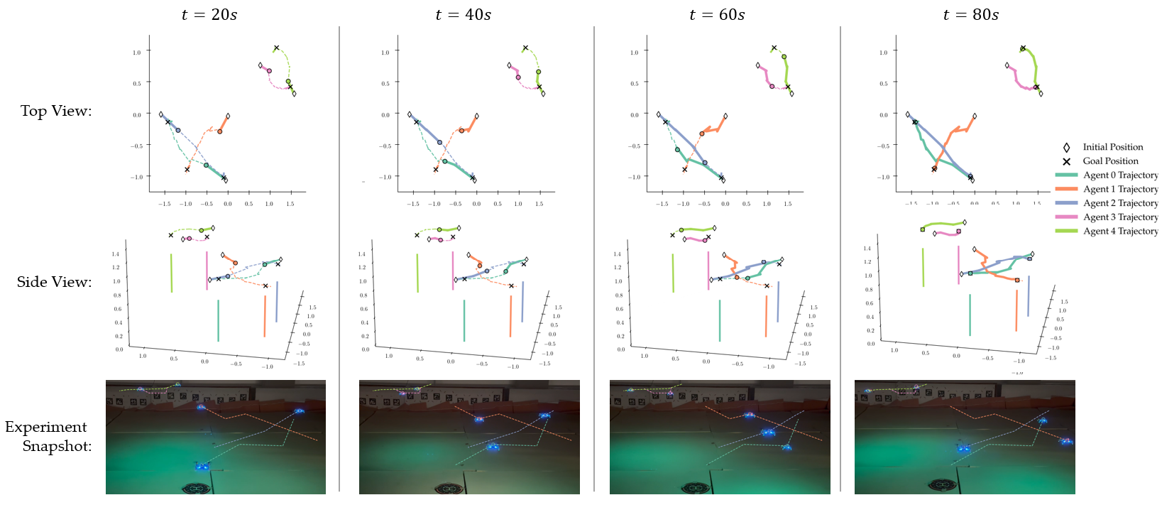
Figure 1: Hardware experiment demonstrated on Crazyflie 2.1 using the Crazyswarm library [1]. In this scenario, five drones navigate around each other in two separate intersections. As time evolves from left to right, the drones are able to safely navigate around each other. The first row depicts the birds-eye view, the middle row depicts the 3D rendered side view, and the lower row shows live pictures of the experiment. The vertical lines correspond to each of the $\times$ markers and denote the $(x,y)$ of the intended goal position colored by agent.

Automatically generating intuitive trajectories in interactive robotic applications involving multiple agents is an important and challenging problem [2]. In situations where scalability matters, we need algorithms that enable robots to safely and tractably navigate around other agents. For example, crowd robot navigation and autonomous driving may require a robot to navigate among multiple humans. Alternatively, drone delivery systems may require quadcopters to navigate by multiple drones in an aerial space. A critical challenge in trajectory planning in such interactive settings is that each robot must account for the likely reactions of other agents to its action, which results in a coupling among the agents, accounting for which quickly becomes intractable as the number of agents increases. In this work, we address this challenge and develop a scalable trajectory optimization algorithm that enables robots to interact efficiently with other robots.

Game-theoretic planning has proven to be a powerful framework for capturing interactions between independent agents [3, 4] where an agent seeks to maximize its utility. Since agents’ utilities depend on the state and actions of all agents, the interaction outcome can be best represented via equilibria that account for the mutual influence of agents. While conceptually powerful, the resulting equilibria are hard to compute as it involves simultaneously solving a set of coupled optimal control problems. Several recent works have developed approximate trajectory optimization algorithms for such games [5, 6, 7]. However, all these works operate in a centralized fashion, i.e. they require the robot to account for interactions with all agents in the environment. As a result, they rarely extend beyond three agents, even for simple dynamics models.

We consider the couplings that result from agents’ interactions in a game-theoretical setup and draw from decentralized and distributed MPC literature to develop a distributed trajectory planner that can be run in a receding horizon fashion efficiently and scalably. We leverage the fact that certain multi-agent interactions are part of a more special class of games, namely dynamic potential games [8]. Potential games are a class of games for which equilibria can be found efficiently and tractably by solving a single optimization problem. Our key insight is that since equilibria of dynamic potential games can be found by minimizing a single potential function, we can apply techniques from distributed and decentralized model predictive control to seek Nash equilibria of game-theoretic interactions in a scalable and efficient manner.

Our algorithm is distributed because each agent independently computes its control input using the state information of its neighboring agents. We compare the performance of our algorithm with a centralized interactive planner in a number of simulation studies and demonstrate that our algorithm can efficiently account for interactions with a larger number of agents. We further showcase the success of our method in hardware experiments involving multiple quadcopters.

The organization of this paper is as follows. In Section II, we review related works. In Section III, we introduce the planning problem to be solved. In Section IV, we discuss the previous work that utilizes dynamic potential games. In Section V, we define our distributed trajectory planning algorithm. In Sections VI and VII, we highlight empirical results in simulations and on hardware. We conclude the paper in Section VIII.

II RELATED WORK

Reactive methods that utilize multi-modal probabilistic prediction models of agents are one of the popular approaches to interactive trajectory planning [9, 10, 11]. The downside with these approaches is that agents are not able to sufficiently influence each other, resulting in conservative interactions. Consequently, several recent methods have considered game-theoretic planning for interactive domains, which enables agents to influence one another and achieve joint prediction and planning. Several approaches that rely on Differential Dynamic Programming have been proposed [12, 13, 5] for finding Nash equilibria of general dynamic games, with [5] demonstrated in real-time. The hierarchical method shown in [14] decomposes the problem into a strategic global planner and a tactical local planner, but it requires discretizing the state and action spaces. Dynamic programming approaches were further utilized in [7] and [15] to approximately find equilibria of interactions under uncertainty. In [16], equilibria of interactive dynamic games were sought under nonlinear state and input constraints. Implicit methods utilize some form of inverse reinforcement learning over trajectory datasets to achieve collision avoidance without directly imposing constraints on the structure of interactions [17, 18, 19], whereas we explicitly take advantage of the structure of certain multi-agent interactions to simplify the problem.

There has been a myriad of approaches exploring the various forms of game-theoretic equilibria among agents. Stackelberg equilibria were initially used to model the outcomes [20, 3, 21]. However, it proved insufficient for general forms of interactions because it assumes a leader-follower structure, which does not apply to non-cooperative games with more than two agents. Due to these challenges, others considered Nash equilibria to capture the interactions among more than two agents.

When it comes to computing equilibria, potential games are a class of games for which equilibria can be found efficiently and reliably. While much of the literature on potential games is oriented toward the static case, there have been several recent advancements in dynamic potential games. Following the pioneering works in [22] and [23], there were initially two primary methods of solving dynamic games: Euler-Lagrange and Pontryagin’s Maximum methods. More recently, a Hamiltonian potential function was explored in [24] in the case of open-loop games for continuous time models. While [25] was primarily focused on communications applications, they demonstrated successful utilization of the simplified problem structure offered by potential games. Similar to our work, [26] posed the idea of connecting the open-loop Nash equilibria of a dynamical game with the solutions to an optimal control problem under certain conditions. Recently, [8] and [27] demonstrated that dynamic potential games can be leveraged for trajectory planning in interactive robotics, but this used a centralized construction.

III Problem Formulation

Consider an interactive trajectory planning problem with $N$ agents. Let $[N]\equiv\{1,\dots,N\}$ be the set of agents’ indices. We refer to the state of the $i$th agent at time $k$ as $x_{k}^{i}\in\mathbb{R}^{n_{i}}$, where $n_{i}$ is the dimension of the state vector of agent $i\in[N]$. Agent $i$’s corresponding control input is denoted as $u_{k}^{i}\in\mathbb{R}^{m_{i}}$, where $m_{i}$ is the dimension of the control space of agent $i\in[N]$. Concatenating the states and inputs of all agents, the full state vector of the system at time $k$ is given by $x_{k}=(x^{1}_{k},x^{2}_{k},\dots,x^{N}_{k})\in\mathbb{R}^{n}$, where $\sum_{i=1}^{N}n_{i}\equiv n$. The concatenated set of control inputs of all agents at time $k$ is similarly denoted by $u_{k}=(u^{1}_{k},u^{2}_{k},\dots,u^{N}_{k})\in\mathbb{R}^{m}$, where $\sum_{i=1}^{N}m_{i}\equiv m$. Generally, subscripts are used to denote the time index, whereas superscripts denote the agent index. The states for agent $i$ across an entire horizon $T$ is notated as $x^{i}=\{x_{0}^{i},\dots,x_{T}^{i}\}\in\mathbb{R}^{n_{i}\times T}$. Similarly, for the controls, let $u^{i}=\{u_{0}^{i},\dots,u_{T}^{i}\}\in\mathbb{R}^{m_{i}\times T}$ be agent $i$’s control inputs across the horizon. We drop both subscript and superscript to refer to all agents over an entire horizon for states $x\in\mathbb{R}^{n\times T}$ and controls $u\in\mathbb{R}^{m\times T}$. Lastly, we use capitalization to differentiate the predicted states $X$ from the actual states $x$ and the same for the controls $U$ from $u$, respectively.

We consider separable agents’ dynamics defined by $f^{i}:\mathbb{R}^{n_{i}}\times\mathbb{R}^{m_{i}}\mapsto\mathbb{R}^{n_{i}}$, i.e. we assume that for every agent $i\in[N]$, we have:

$$x^{i}_{k+1}=f^{i}(x^{i}_{k},u^{i}_{k}).$$ (1)

We denote the strategy space of each agent $i\in[N]$ as $\Gamma^{i}$. Let the strategy $\gamma^{i}\in\Gamma^{i}$ of agent $i$ be given by $\gamma^{i}:\mathbb{R}^{n_{i}}\times\{0,1,\ldots,T-1\}\mapsto\mathbb{R}^{m_{i}}$ which determines the actions of agent $i$ at all time instants. We consider open-loop strategies that are only a function of the system’s initial state and the time step. Therefore, we have $\gamma^{i}(x_{0},k):=u^{i}_{k}$. Hence, for simplicity, we use strategies and actions interchangeably here out.

We assume that each agent $i$ is minimizing some cost $J^{i}(\cdot)$ over the time horizon $T$:

$$J^{i}(x_{0},\gamma)=S^{i}(x_{T},T)+\sum_{k=0}^{T-1}L^{i}(x_{k},\gamma(x_{0},k),k),$$ (2)

where $S^{i}(\cdot)$ is the terminal cost of agent $i$ and $L^{i}(\cdot)$ is the running cost of agent $i$. Note that the cost perceived by an agent $i$ may depend on the states and actions of all the other agents. As a result, generally, it is not possible for all agents to optimize their costs simultaneously, and we need to model the outcome of the interactions between the agents as equilibria of the underlying dynamic game. We denote our dynamic games by a compact notation, $G_{x_{0}}^{T}:=(T,\{\gamma^{i}\}_{i=1}^{N},\{J^{i}\}_{i=1}^{N},\{f^{i}\}_{i=1}^{N}),$ which denotes the dynamic game that arises from interactions of the agents over a horizon $T$ starting from the initial condition $x_{0}$.

Let $\gamma^{-i}=(\gamma^{1},\dots,\gamma^{i-1},\gamma^{i+1},\dots,\gamma^{N})$ denote the strategies of all other agents except $i$. We use similar notation to express the states and controls of all other agents except $i$ for a given time step $k$ as $x_{k}^{-i}\in\mathbb{R}^{n-n_{i}}$ and $u_{k}^{-i}\in\mathbb{R}^{m-m_{i}}$, respectively. Then, the Nash equilibria of our dynamic game are defined as [28]:

Definition 1.

For a given game, $G_{x_{0}}^{T}:=(T,\{\gamma^{i}\}_{i=1}^{N},\{J^{i}\}_{i=1}^{N},\{f^{i}\}_{i=1}^{N})$, a set of strategies $\gamma^{*}$ are open-loop Nash equilibrium strategies if for every agent $i\in[N]$ and every strategy $\gamma^{i}$, we have

$$J^{i}(x_{0},\gamma^{*})\leq J^{i}(x_{0},{\gamma^{i}},{\gamma^{-i*}}).$$ (3)

Definition 1 implies that at equilibrium, no agent has any incentive for changing its strategy and actions once it fixes the strategies and actions of all the other agents to be their equilibrium strategies $\gamma^{-i*}$. However, finding Nash equilibria is challenging, as solving (3) requires solving a set of coupled optimal control problems. Finding equilibria has proven difficult even in two-player settings for discrete state and action spaces [29, 30, 31]. Most recent methods for finding Nash equilibria of dynamic games that arise in robotics [5, 8, 6] solve the game in a centralized fashion, i.e. each agent must maintain a full copy of all the other agents. As a result, the existing methods and solvers are not scalable and become intractable beyond three agents with simple dynamics. In this work, we seek to remedy this and develop a distributed trajectory optimization algorithm for finding Nash equilibria of dynamic games underlying multi-agent interactions.

IV Prior Results

In this section, we review some of the results from our previous work that we will utilize in the current work. Specifically, we review our previous results from [8] that allow one to bypass solving (3) for interactions that are dynamic potential games [32]. More specifically, we have the following result from [8].

Theorem 1.

For a given dynamic game $G_{x_{0}}^{T}=(T,\{\gamma^{i}\}_{i=1}^{N},\{J^{i}\}_{i=1}^{N},\{f^{i}\}_{i=1}^{N})$, if for each agent $i\in[N]$, the running and terminal costs have the the following structure

$$L^{i}(x_{k},u_{k})=p(x_{k},u_{k})+c^{i}(x_{k}^{-i},u_{k}^{-i}),\;\forall k$$ (4)

and

$$S^{i}(x_{T})=\bar{s}(x_{T})+s^{i}(x^{-i}_{T}),$$ (5)

then, the dynamic game $G_{x_{0}}^{T}$ is a dynamic potential game. and open-loop Nash equilibria $u^{*}=(u^{1*},\dots,u^{N*})$ can be found by solving the following optimal control problem

$$\begin{split}&\min_{u}\sum_{k=0}^{T-1}p(x_{k},u_{k})+\bar{s}(x_{T}),\\ &\text{s.t. }x_{k+1}^{i}=f^{i}(x_{k}^{i},u_{k}^{i}).\\ \end{split}$$ (6)

Conditions (4) and (5) imply that one can decompose both the running costs $L^{i}(\cdot)$ and terminal costs $S^{i}(\cdot)$ into potential functions $p(\cdot)$ and $\bar{s}(\cdot)$ which can depend on the full state and control vector of the agents, and the cost terms $c^{i}(\cdot)$ and $s^{i}(\cdot)$ that have no dependence on the state and control input of agent $i$.

For the remainder of the section, we make this result more concrete via a navigation example, which serves as our running example throughout the paper.

Consider a multi-agent navigation setup where each agent $i\in[N]$ must reach a goal state $\bar{x}^{i}$. We assume that each agent’s running cost function is composed of a tracking cost and a control penalty term defined as:

$$\begin{split}C^{i}_{tr}(x_{k}^{i},u_{k}^{i})&=(x_{k}^{i}-\bar{x}^{i})^{\intercal}Q^{i}(x_{k}^{i}-\bar{x}^{i})\\ &+(u_{k}^{i}-\bar{u}^{i})^{\intercal}R^{i}(u_{k}^{i}-\bar{u}^{i}),\end{split}$$ (7)

$$C^{i}_{tr,T}(x_{T}) =(x^{i}_{T}-\bar{x}^{i})^{\intercal}Q_{f}^{i}(x^{i}_{T}-\bar{x}^{i}),$$ (8)

where $Q^{i},Q_{f}^{i}\in\mathbb{R}^{n_{i}\times n_{i}}$, $Q^{i},Q_{f}^{i}\succeq 0$ and $R^{i}\in\mathbb{R}^{m_{i}\times m_{i}}$, $R^{i}\succ 0$ are all symmetric matrices, and $\bar{u}^{i}$ is a reference control input. Moreover, assume that agents’ decisions are coupled through cost terms such as the collision avoidance terms between any pair of agents $i\neq j,i,j\in[N]$ defined as:

$$C^{ij}_{ca}(x_{k}^{i},x_{k}^{j})=\alpha^{ij}(d(x_{k}^{i},x_{k}^{j})),$$ (9)

where $d(x_{k}^{i},x_{k}^{j})\equiv d_{k}^{ij}$ is the distance between agents $i$ and $j$ at time $k$.

For each agent $i\in[N]$, the instantaneous running cost $L^{i}(\cdot)$ can then be defined as:

$$L^{i}(x_{k},u_{k}^{i})=C^{i}_{tr}(x_{k}^{i},u_{k}^{i})+\sum_{i\neq j}^{N}C^{ij}_{ca}(x_{k}^{i},x_{k}^{j}).$$ (10)

It was shown in [8] that under the assumption that agents induce coupling costs between each other symmetrically, i.e. $C^{ij}_{ca}(x_{k}^{i},x_{k}^{j})=C^{ji}_{ca}(x_{k}^{j},x_{k}^{i}),\forall i\neq j\in[N]$, the dynamic game is a dynamic potential game with the potential function:

$$p(x_{k},u_{k})=\sum_{i=1}^{N}C^{i}_{tr}(x^{i}_{k},u^{i}_{k})+\sum_{i=1,i<j}^{N}C^{ij}_{ca}(x^{i}_{k},x^{j}_{k}).$$ (11)

This implies that Nash Equilibria (3) can be found by solving (6), which is a single optimal control problem. Prior work [8] used iLQR [33, 34] for minimizing (11) in a Model Predictive Control (MPC) setting. Explicitly, it solves (6) for all agents iteratively as covered in Algorithm 1. We refer the reader to the original work [8] for additional details.

Algorithm 1 Potential-iLQR

  Inputs

  dynamics $\{f^{i}\}_{i=1}^{N}$, potentials $p$ and $\bar{s}$, initial state $x_{0}$

  Outputs

  control inputs $u$

  Initialization

  $u\leftarrow 0^{N\times m}$

1.  while not converged do

2.     Rollout from $x_{0}$ with $u$ s.t. (1) to compute $X$

3.     Linearize dynamics, quadraticize costs about $X,u$

4.     Solve the Riccati recursion to update controls $u$

5.  end while

V Distributed Interactive Trajectory Optimization

Prior work has proposed to solve (11) by requiring every agent to maintain a copy of all the other agents, which restricts the scalability of the method. Our key insight is that we can solve the optimal control problem (11) more efficiently using ideas from distributed MPC [35, 36, 37, 38]. Specifically, we can break up (11) into smaller subproblems more relevant to each agent.

To formalize distributed interactive trajectory planning, we borrow ideas from [37] and [39] and introduce the concept of an interaction graph $\mathcal{G}=\{\mathcal{V},\mathcal{E}\}$ comprising nodes $\mathcal{V}=[N]$ for each agent $i$ and edges $\mathcal{E}\in\mathcal{V}\times\mathcal{V}$, where each edge $(i,j)\in\mathcal{V}$, indicates a coupling between two agents in their costs. For our purposes, these edges are connected if agents ever get within a proximity distance $d_{\text{prox}}$ of each other throughout the predicted trajectories. Formally, let $\{d^{ij}_{k}\}_{k=0}^{T-1}\in\mathbb{R}^{T}$ be the predicted distances between agents $i$ and $j$ over the horizon $T$. We create a bidirectional edge $(i,j)$ if:

$$\exists k,0\leq k<T,\;\text{such that}\;d^{ij}_{k}<\alpha d_{\text{prox}},$$ (12)

where $\alpha\in\mathbb{R},\alpha\geq 1$ is some aggressiveness parameter on how finely to split up the graph. For sufficiently large $\alpha$, the interaction graph is complete, i.e., all agents are connected with one another. Whereas for sufficiently small $\alpha$, $\mathcal{E}=\emptyset$. Additionally, for each agent $i\in[N]$, its set of neighbors is defined as $\mathcal{N}^{i}$, such that $\mathcal{N}^{i}=\{j:(i,j)\in\mathcal{E}\}$ (see Fig. 2). The introduction of the interaction graph is motivated by human swarm motion. As referenced in [40], the key to collective motion is a pedestrian’s zone of influence. Intuitively, humans need not worry about others outside their vicinity. Similarly, we argue that in multi-agent interactions, agents need only pay attention to their zone of influence in the navigation problem.

Figure 2: Schematic Example of an interaction graph for one-time step, where $\mathcal{N}^{1}=\{2,3\}$, $\mathcal{N}^{2}=\{1,3,4\}$, $\mathcal{N}^{3}=\{1,2\}$, $\mathcal{N}^{4}=\{2,5\}$, and $\mathcal{N}^{5}=\{4\}$.

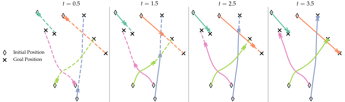
Figure 3: Example trajectories of DP-iLQR (Algorithm 2) for unicycle dynamics for varying numbers of agents from random initial conditions and goal positions. As time progresses from the left to right, the algorithm is able to guide agents through complex interactions.

We require each agent $i$ to solve its own subproblem, which we denote by $\mathcal{P}^{i}$, associated with minimizing the potential function that comprises only itself and its neighbors $\tilde{p}^{i}$, i.e., the subset of the graph that it shares edges with $\mathcal{N}^{i}$. Let the full subproblem consist of agents in the set $\widetilde{\mathcal{N}}^{i}=\mathcal{N}^{i}\cup i$. The state vector of this subproblem at time $k$ is then denoted by $\tilde{x}_{k}^{i}=\{x_{k}^{j}\}_{j\in\widetilde{\mathcal{N}}^{i}}$ with the corresponding control input $\tilde{u}_{k}^{i}=\{u_{k}^{j}\}_{j\in\widetilde{\mathcal{N}}^{i}}$. We propose to divide the centralized problem (6) into a set of local subproblems, where each agent $i$ solves its subproblem $\mathcal{P}^{i}$ defined as

$$\begin{split}&\min_{\tilde{u}^{i}}\sum_{k=0}^{T-1}\tilde{p}^{i}(\tilde{x}^{i}_{k},\tilde{u}^{i}_{k})+\tilde{\bar{s}}^{i}(\tilde{x}^{i}_{T})\\ &\text{s.t. }x^{i}_{k+1}=f^{i}(x^{i}_{k},u^{i}_{k}),\\ \end{split}$$ (13)

where $\tilde{\bar{s}}^{i}(\cdot):\mathbb{R}^{\tilde{n}_{i}}\mapsto\mathbb{R}$ for $\tilde{n}_{i}=\sum_{i\in\tilde{N}_{i}}n_{i}$, is a terminal cost for the local problem. Therefore, (13) is the local analog to (6) with local potential functions $\tilde{p}^{i}$ and $\tilde{\bar{s}}^{i}$ that comprise local costs. In the specific case of multi-agent navigation, one such potential function could take the following form:

$$\tilde{p}^{i}(x_{k},u_{k})=\sum_{j\in\widetilde{\mathcal{N}}^{i}}C^{j}_{tr}(x^{j}_{k},u^{j}_{k})+\sum_{j\in\mathcal{N}^{i}}C^{ij}_{ca}(x^{i}_{k},x^{j}_{k}).$$ (14)

Hence, (14) is then a subset of (11) that takes advantage of the sparsity of the interaction graph.

Let the trajectory of the full system predicted by agent $i$ at time $k$ be $X^{i}_{k}$, where $X^{i}_{0}\equiv x_{0}$, such that over the full horizon:

$$X^{i}=\{x_{0},X^{i}_{1},\dots,X^{i}_{T-1}\},$$ (15)

where $X^{i}\in\mathbb{R}^{n\times T}$ is the predicted trajectory according to agent $i$ across the horizon. We are now ready to define our distributed trajectory planner in Algorithm 2 — Distributed Potential-iLQR (DP-iLQR).

Algorithm 2 DP-iLQR

  Inputs

  predicted trajectories $X^{i}$ (15), system dynamics $\{f^{j}\}_{j=1}^{N}$ (1), costs eqs. 7 to 9

  Outputs

  control inputs $u^{i}$ for agent $i$

1.  $\mathcal{N}^{i},\tilde{x}_{0}^{i}\leftarrow\text{define Interaction Graph}(X^{i})$  (12)

2.  $\tilde{p}^{i},\tilde{\bar{s}}^{i}\leftarrow\text{define local potential functions}(\mathcal{N}^{i})$

3.  $U\leftarrow\text{Potential-iLQR}(\{f^{i}\}_{i\in\widetilde{\mathcal{N}}_{i}},\tilde{p}^{i},\tilde{\bar{s}}^{i},\tilde{x}_{0}^{i})$ (Alg. 1)

4.  $u^{i}\leftarrow$ extract Agent$(U,i)$

In applying Algorithm 2 in a receding horizon fashion, we continually compute the interaction graph at each step in line 1 and compose local potential functions in line 2. Agents then solve their local subproblem (13) in line 3. Agent $i$’s solution $u^{i}$ is then pulled out from $U$ in line 4 and executed. This is then communicated with the rest of the system to define the subsequent graph at the next step.

We can utilize any single-agent trajectory optimization algorithm to solve each local subproblem by each agent $i$. We choose iLQR for solving each subproblem $\mathcal{P}^{i}$ due to its widespread success across many robotics domains. The broader question of how these sub-problems interact with each other remains an open question, which we will explore empirically in Section VI.

VI SIMULATION STUDIES

To evaluate the performance of DP-iLQR, we execute the algorithm in a series of Monte Carlo simulations. We would like to show that DP-iLQR can handle larger-sized problems than Potential-iLQR. To accomplish this, we vary the number of agents and compare the centralized planner with the distributed planner at a given initial condition. We considered a multi-agent navigation setup with several different dynamics models, including 2D double integrator, 2D unicycle, and 3D quadcopter dynamics. We model our quadcopter as a six-dimensional model, specifically:

$$\dot{p}_{x} =v_{x}, \dot{v}_{x} =g\tan(\theta),$$ (16)

$$\dot{p}_{y} =v_{y}, \dot{v}_{y} =-g\tan(\phi),$$

$$\dot{p}_{z} =v_{z}, \dot{v}_{z} =\tau-g,$$

where $\theta$ is the pitch, $\phi$ is the roll, $\tau$ is the combined force of the motors in the z-direction, $p_{x}$, $p_{y}$, and $p_{z}$ are the 3D position, $v_{x}$, $v_{y}$, and $v_{z}$ are the 3D velocities, and $g$ is the acceleration due to gravity.

The specific form of collision avoidance cost that we utilized is the following:

$$\alpha^{ij}(d_{k}^{ij})=\begin{cases}\beta(d_{k}^{ij}-d_{\text{prox}})^{2}&d_{k}^{ij}<d_{\text{prox}}\\ 0&\text{ otherwise},\end{cases}$$ (17)

where $\beta\in\mathbb{R}$ is some weighting parameter and $d_{\text{prox}}$ is a threshold distance where agents begin incurring penalties for being too close to each other.

We implemented Algorithm 2 in a combination of Python and C++. We generated 30 random initial conditions. For a given initial condition, we fixed the number of agents and computed the interactive trajectories of the agents using both Potential-iLQR and DP-iLQR. We implemented our algorithm in a receding horizon controller to fully exercise Algorithm 2. We ran the simulations with a horizon length of 40, a time interval of 0.1 seconds, and a collision radius $d_{\text{prox}}$ of 0.5 meters. As shown in Fig. 3, DP-iLQR generates intuitive collision-free trajectories under feasible initial conditions.

We conducted two primary analyses to quantify the differences in the performance between the centralized and distributed implementations: limited and unlimited solve time. The solve time refers to the time it takes at a given operating point to entirely execute the control algorithm, which corresponds to the time the algorithm would need to provide a new control input in real-time use cases.

VI-A Analysis 1 - Unlimited Solve Time

For the case of unlimited solve time, we enforce no computational time limit on the solver for converging to a solution at each receding horizon. This is an unrealistic assumption for practical implementations, but it enables us to compare the solve time of the two methods. In Fig. 4, we compare the individual subproblem solve times throughout the simulated trajectories. As the number of agents increases, the problem gets increasingly congested; hence, we see each agent spending more time computing its subsequent control input. This is to be expected as the size of the state space grows and the cost surface becomes more challenging to navigate. The advantage of DP-iLQR in terms of the solve time is most prominent for simpler dynamical models like the double integrator. Regardless, it demonstrates a consistent decrease in solve time that widens with more agents.

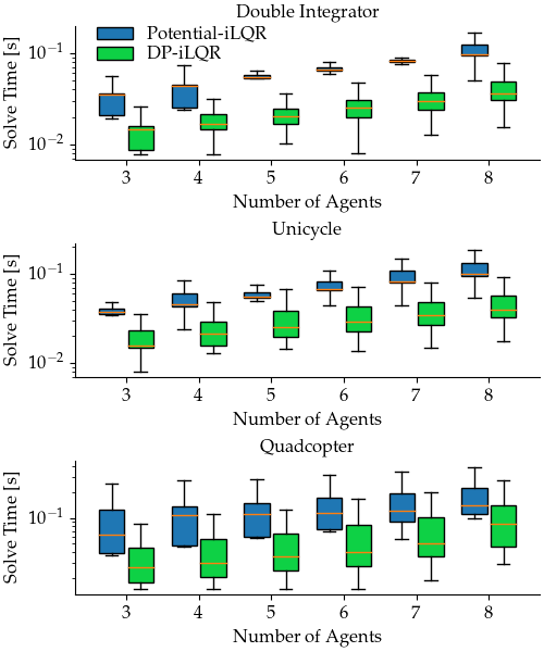
Figure 4: Average solve times without real-time constraints. DP-iLQR yields a consistently lower solve time than the centralized solver across various dynamics models and numbers of agents.

VI-B Analysis 2 - Real-Time Constraint

When evaluating performance with more realistic timing constraints, we only permit the solver to iterate until it exceeds some time-based threshold. This serves as a ’best-effort’ solution that will be more applicable to a hardware implementation where the MPC planner requires a solution by the end of each time step. In this case, we compare the quality of the trajectories under real-time constraints. In particular, we measure the distance to goal at the end of the time horizon as a measure of solution quality. Fig. 5 demonstrates the distance to the goal position under the two methods for various numbers of agents.

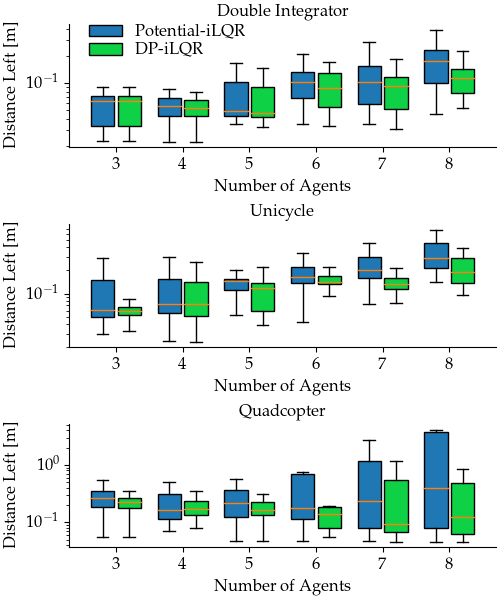
Figure 5: Average distance left to the goal position with a real-time constraint. While the difference between the two solvers is smaller at lower scales, Potential-iLQR is unable to maintain the quality of trajectories at the scales of six or more agents.

As the number of agents exceeds six, we see in Fig. 5 that the variance in the centralized solver increases significantly as it starts getting overwhelmed handling the multitude of agent interactions. In contrast, the distributed solver shows much more consistent convergence statistics and even outperforms the centralized solver in most cases.

VII EXPERIMENTS

To evaluate the real-time capabilities of our algorithm, we conducted navigation experiments involving multiple quadcopters. We ran the DP-iLQR algorithm on five Crazyflie 2.1 quadcopters, where each quadcopter navigates to its designated final position. VICON motion capture system was used to provide position and velocity feedback to all the quadcopters. The position update computed by DP-iLQR was sent to each quadcopter online via the Crazyswarm API [1]. The algorithm was executed offboard on a laptop with an 8-core AMD processor with 32 GB of RAM. We demonstrated that DP-iLQR provides a more stable and intuitive trajectory than the Potential iLQR [8]. A visualization demonstrating the near-real-time trajectories generated by DP-iLQR is shown in Fig. 1.

VIII CONCLUSION

Summary. We introduced a scalable and distributed algorithm for interactive trajectory planning in multi-agent interactions. We considered interactions in a game-theoretic setting and utilized the connection between multi-agent interactions and potential games to reduce the problem of finding equilibria of the game to that of minimizing a single potential function. Then, we used distributed trajectory optimization algorithms to minimize the resulting potential function. This results in a scalable and efficient trajectory planner for finding equilibria of interactive dynamic games. We compared our method with the state-of-the-art in several simulation studies and hardware experiments involving multiple quadcopters.

Limitations and Future Work. In our simulations and experiments, we found that the consistency of the trajectory that results from DP-iLQR is sensitive to the choice of cost parameters. More work would be required to investigate the feasibility of designing a self-tuning algorithm to determine optimal weights automatically. We would like to further examine both the theoretical guarantees and optimality gap of our proposed trajectory planner, as well as the application and impacts of distributed optimization techniques such as ADMM on distributed interactive trajectory planning.

References

- [1] J. A. Preiss, W. Honig, G. S. Sukhatme, and N. Ayanian, “Crazyswarm: A large nano-quadcopter swarm,” in 2017 IEEE International Conference on Robotics and Automation (ICRA), pp. 3299–3304, 2017.
- [2] G.-Z. Yang, J. Bellingham, P. E. Dupont, P. Fischer, L. Floridi, R. Full, N. Jacobstein, V. Kumar, M. McNutt, R. Merrifield, B. J. Nelson, B. Scassellati, M. Taddeo, R. Taylor, M. Veloso, Z. L. Wang, and R. Wood, “The grand challenges of science robotics,” Science Robotics, vol. 3, no. 14, p. eaar7650, 2018.
- [3] D. Sadigh, S. Sastry, S. A. Seshia, and A. D. Dragan, “Planning for autonomous cars that leverage effects on human actions.,” in Robotics: Science and systems, vol. 2, pp. 1–9, Ann Arbor, MI, USA, 2016.
- [4] Z. Wang, R. Spica, and M. Schwager, “Game theoretic motion planning for multi-robot racing,” in Distributed Autonomous Robotic Systems, pp. 225–238, Springer, 2019.
- [5] D. Fridovich-Keil, E. Ratner, L. Peters, A. D. Dragan, and C. J. Tomlin, “Efficient iterative linear-quadratic approximations for nonlinear multi-player general-sum differential games,” 2019.
- [6] F. Laine, D. Fridovich-Keil, C.-Y. Chiu, and C. Tomlin, “The computation of approximate generalized feedback nash equilibria,” arXiv preprint arXiv:2101.02900, 2021.
- [7] M. Wang, N. Mehr, A. Gaidon, and M. Schwager, “Game-theoretic planning for risk-aware interactive agents,” in 2020 IEEE/RSJ International Conference on Intelligent Robots and Systems (IROS), pp. 6998–7005, IEEE, 2020.
- [8] T. Kavuncu, A. Yaraneri, and N. Mehr, “Potential ilqr: A potential-minimizing controller for planning multi-agent interactive trajectories,” 2021.
- [9] E. Schmerling, K. Leung, W. Vollprecht, and M. Pavone, “Multimodal probabilistic model-based planning for human-robot interaction,” CoRR, vol. abs/1710.09483, 2017.
- [10] H. Nishimura, B. Ivanovic, A. Gaidon, M. Pavone, and M. Schwager, “Risk-sensitive sequential action control with multi-modal human trajectory forecasting for safe crowd-robot interaction,” CoRR, vol. abs/2009.05702, 2020.
- [11] H. Bai, S. Cai, N. Ye, D. Hsu, and W. S. Lee, “Intention-aware online pomdp planning for autonomous driving in a crowd,” in 2015 IEEE International Conference on Robotics and Automation (ICRA), pp. 454–460, 2015.
- [12] W. Sun, E. A. Theodorou, and P. Tsiotras, “Game theoretic continuous time differential dynamic programming,” in 2015 American control conference (ACC), pp. 5593–5598, IEEE, 2015.
- [13] B. Di and A. Lamperski, “Differential dynamic programming for nonlinear dynamic games,” 2018.
- [14] J. F. Fisac, E. Bronstein, E. Stefansson, D. Sadigh, S. S. Sastry, and A. D. Dragan, “Hierarchical game-theoretic planning for autonomous vehicles,” in 2019 International Conference on Robotics and Automation (ICRA), pp. 9590–9596, IEEE, 2019.
- [15] N. Mehr, M. Wang, M. Bhatt, and M. Schwager, “Maximum-entropy multi-agent dynamic games: Forward and inverse solutions,” IEEE Transactions on Robotics, 2023.
- [16] S. L. Cleac’h, M. Schwager, and Z. Manchester, “Algames: A fast solver for constrained dynamic games,” arXiv preprint arXiv:1910.09713, 2019.
- [17] B. D. Ziebart, N. Ratliff, G. Gallagher, C. Mertz, K. Peterson, J. A. Bagnell, M. Hebert, A. K. Dey, and S. Srinivasa, “Planning-based prediction for pedestrians,” in 2009 IEEE/RSJ International Conference on Intelligent Robots and Systems, pp. 3931–3936, 2009.
- [18] P. Henry, C. Vollmer, B. Ferris, and D. Fox, “Learning to navigate through crowded environments,” in 2010 IEEE International Conference on Robotics and Automation, pp. 981–986, 2010.
- [19] H. Kretzschmar, M. Spies, C. Sprunk, and W. Burgard, “Socially compliant mobile robot navigation via inverse reinforcement learning,” The International Journal of Robotics Research, vol. 35, no. 11, pp. 1289–1307, 2016.
- [20] J. H. Yoo and R. Langari, “Stackelberg game based model of highway driving,” in Dynamic Systems and Control Conference, vol. 45295, pp. 499–508, American Society of Mechanical Engineers, 2012.
- [21] A. Liniger and J. Lygeros, “A noncooperative game approach to autonomous racing,” IEEE Transactions on Control Systems Technology, vol. 28, no. 3, pp. 884–897, 2019.
- [22] D. Dechert, “Optimal control problems from second-order difference equations,” Journal of Economic Theory, vol. 19, no. 1, pp. 50–63, 1978.
- [23] W. D. Dechert and S. O’Donnell, “The stochastic lake game: A numerical solution,” Journal of Economic Dynamics and Control, vol. 30, no. 9-10, pp. 1569–1587, 2006.
- [24] D. Dragone, L. Lambertini, G. Leitmann, and A. Palestini, “Hamiltonian potential functions for differential games,” Automatica, vol. 62, pp. 134–138, 2015.
- [25] S. Zazo, S. Valcarcel Macua, M. Sánchez-Fernández, and J. Zazo, “Dynamic potential games with constraints: Fundamentals and applications in communications,” IEEE Transactions on Signal Processing, vol. 64, no. 14, pp. 3806–3821, 2016.
- [26] W. D. Dechert, “Non cooperative dynamic games: a control theoretic approach,” Unpublished. Available on request to the author, 1997.
- [27] M. Bhatt, A. Yaraneri, and N. Mehr, “Efficient constrained multi-agent interactive planning using constrained dynamic potential games,” arXiv preprint arXiv:2206.08963, 2022.
- [28] T. Başar and G. J. Olsder, Dynamic Noncooperative Game Theory, 2nd Edition. Society for Industrial and Applied Mathematics, 1998.
- [29] A. Fabrikant, C. Papadimitriou, and K. Talwar, “The complexity of pure nash equilibria,” in Proceedings of the thirty-sixth annual ACM symposium on Theory of computing, pp. 604–612, 2004.
- [30] M. Ummels, “The complexity of nash equilibria in infinite multiplayer games,” in International Conference on Foundations of Software Science and Computational Structures, pp. 20–34, Springer, 2008.
- [31] C. Daskalakis, P. W. Goldberg, and C. H. Papadimitriou, “The complexity of computing a nash equilibrium,” SIAM Journal on Computing, vol. 39, no. 1, pp. 195–259, 2009.
- [32] A. Fonseca-Morales and O. Hernández-Lerma, “Potential differential games,” Dynamic Games and Applications, vol. 8, no. 2, pp. 254–279, 2018.
- [33] W. Li and E. Todorov in Iterative Linear Quadratic Regulator Design for Nonlinear Biological Movement Systems., vol. 1, pp. 222–229, 01 2004.
- [34] Y. Tassa, T. Erez, and E. Todorov, “Synthesis and stabilization of complex behaviors through online trajectory optimization,” in 2012 IEEE/RSJ International Conference on Intelligent Robots and Systems, pp. 4906–4913, 2012.
- [35] E. Camponogara, D. Jia, B. Krogh, and S. Talukdar, “Distributed model predictive control,” IEEE Control Systems Magazine, vol. 22, no. 1, pp. 44–52, 2002.
- [36] Y. Zheng, S. E. Li, K. Li, F. Borrelli, and J. K. Hedrick, “Distributed model predictive control for heterogeneous vehicle platoons under unidirectional topologies,” IEEE Transactions on Control Systems Technology, vol. 25, no. 3, pp. 899–910, 2017.
- [37] T. Keviczky, F. Borrelli, and G. J. Balas, “Decentralized receding horizon control for large scale dynamically decoupled systems,” Automatica, vol. 42, no. 12, pp. 2105–2115, 2006.
- [38] A. Richards and J. How, “Decentralized model predictive control of cooperating uavs,” in 2004 43rd IEEE Conference on Decision and Control (CDC) (IEEE Cat. No.04CH37601), vol. 4, pp. 4286–4291 Vol.4, 2004.
- [39] G. Ferrari-Trecate, L. Galbusera, M. P. E. Marciandi, and R. Scattolini, “Model predictive control schemes for consensus in multi-agent systems with single- and double-integrator dynamics,” IEEE Transactions on Automatic Control, vol. 54, no. 11, pp. 2560–2572, 2009.
- [40] W. H. Warren, “Collective motion in human crowds,” Current Directions in Psychological Science, vol. 27, no. 4, pp. 232–240, 2018.