Pole-skipping points in 2D gravity and SYK model

Abstract

We represent the first investigation of pole-skipping on both the gravity and field theory sides. In contrast to the higher dimensional models, there is no momentum degree of freedom in $(1+1)-$dimensional bulk theory. Thus, we then consider a scalar field mass as our degree of freedom for the pole-skipping phenomenon instead of momentum. The pole-skipping frequencies of the scalar field in 2D gravity are the same as higher dimensional cases: $\omega=-i2\pi Tn$ for positive integers $n$. At each of these frequencies, there is a corresponding pole-skipping mass, so the pole-skipping points exist in $(\omega,m)$ space. We also compute the pole-skipping points of the SYK model in $(\omega,h)$ space where $h$ is the dimension of the bilinear primary operator. We find that there is a one-to-one correspondence of the pole-skipping points between the JT gravity and the SYK model. To obtain the pole-skipping points, we need to consider the parameter $\epsilon$ related to the chemical potential on the horizon of charged JT gravity and the particle-hole asymmetric parameter $\mathcal{E}$ of the complex SYK model as shift parameters. This highlights the $\epsilon-\mathcal{E}$ correspondence in relation to pole-skipping phenomenon.

1 Introduction

The AdS/CFT correspondence maldacena ; witten1 ; witten2 ; gubser provides a useful method to compute Green’s functions in strongly coupled quantum many-body systems casalderrey ; natsuume ; ammon ; zaanen ; hartnoll . In recent years, pole-skipping, an interesting property that occurs in the Green’s function, has been studied in much of the literature Grozdanov1 ; Blake1 ; Grozdanov2 ; Makoto1 ; Makoto2 ; BlakeDavison ; Das ; Abbasi2 ; Abbasi1 ; Choi ; Karunava ; Yongjun2 ; Mahdi . The pole-skipping phenomenon is a mathematical property that the retarded Green’s function is not unique at some points in the complex momentum space $(\omega,k)$. From now on, we call those points pole-skipping points. Generally, the retarded Green’s function takes a form

$$G^{R}(\omega,k)=\frac{b(\omega,k)}{a(\omega,k)}\,.$$ (1)

At a pole-skipping point $(\omega_{\star},k_{\star})$, both $a$ and $b$ satisfy $a(\omega_{\star},k_{\star})=b(\omega_{\star},k_{\star})=0$, and the retarded Green’s function becomes ill-defined. So, if we find the intersections of zeros and poles in the retarded Green’s functions, we can obtain pole-skipping points. For the theories with the holographic duals, we can use a simpler method to obtain the pole-skipping points from the bulk field equation Makoto1 ; Makoto2 ; BlakeDavison . The absence of a unique incoming mode at the black hole horizon leads to the nonuniqueness of the Green’s function on the boundary. For the static black holes, the leading pole-skipping frequency $\omega$ is given by Makoto3 ; N1 ; Yuan1 ; N2 ; Yuan2 ; Diandian

$$\omega=2\pi iT(s-1),$$ (2)

where $i$ is the imaginary unit, and $s$ denotes the spin of the operator. For instance, it has been noted that pole-skipping points in the upper-half $\omega$-plane are linked to quantum chaos and are closely related to hydrodynamics. In the maximally chaotic systems, the Lyapunov exponent $\lambda$ and the butterfly velocity $v_{B}$ can be extracted from the leading pole-skipping point of the metric fluctuation ($s=2$) Grozdanov1 ; Blake1 ; Blake3 ; Jeong . For other fluctuations ($s=0,1/2,1,3/2$), the leading pole-skipping points are not related to the maximal chaos N2 .

The Jackiw-Teitelboim (JT) gravity is a two-dimensional theory of gravity coupled to a dilaton, and describes the near horizon dynamics of near extremal black holes Jackiw ; Teitelboim . The Sachdev-Ye-Kitaev (SYK) model is a strongly interacting quantum system at low energy. It has some interesting properties: It is solvable at the large $N$ limit with an emergent conformal symmetry Sachdev ; Kitaev . The SYK model is maximally chaotic so that the Lyapunov exponent saturates the Maldacena-Shenker-Stanford(MSS) bound $\lambda=2\pi T$ Maldacena:2015waa ; Jensen . Symmetries and reparametrization connect the SYK model to the AdS₂ horizon. Near the horizon of an AdS₂ black hole corresponds to the IR of Majorana SYK Maldacena . JT gravity has a nearly AdS₂ geometry, and its conformal symmetry is slightly broken. The Schwarzian action can be derived for JT gravity by spontaneously breaking the reparametrization symmetry down to $SL(2,\mathbb{R})$ Sarosi . Similarly, the Majorana SYK model also has its conformal symmetry spontaneously broken to $SL(2,\mathbb{R})$ due to reparametrization, allowing for the calculation of the Schwarzian action Stanford ; Polchinski . The effective action can be obtained from both gravity theory on the boundary and the Majorana SYK model. Therefore, JT gravity has been considered as the gravitational dual of the Majorana SYK model. In the bulk gravity models, there are also various analogies to the complex SYK model csyk1 ; csyk2 . For example, for nearly AdS₂ in JT gravity with $SL(2,L)\times U(1)$ symmetry, it is holographically dual to the complex SYK model Godet .

Pole-skipping has primarily been studied on the gravity side thus far Grozdanov1 ; Blake1 ; Grozdanov2 ; Makoto1 ; Makoto2 ; BlakeDavison . In the case of the (1+1)-dimensional SYK chain, it has been discovered that pole-skipping is determined by the stress tensor’s contribution to many-body chaos, even when it is not at its maximum Choi . However, up to now, there are few works that reported the pole-skipping points on both the gravity and field theory sides in previous literature. There have been no findings regarding the connection between pole-skipping points in the SYK model and those in JT gravity.

In this paper, we aim to fill this gap. Note that the Green’s functions of the JT gravity and SYK model do not depend on momentum $k$ because there is no spatial coordinate as they are $(0+1)-$dimensional field theories. In the absence of momentum $k$, one way to define the pole-skipping points is to identify the mass $m$ as a variable of the Green’s function. Following Ref. Ahn:2020bks , we compute the pole-skipping points in the $(\omega,m)$ space in three ways: 1) near horizon analysis 2) analytic bulk solution for the JT gravity, and 3) conformal two-point function of the SYK model. We have obtained consistent results by all three methods and found a one-to-one correspondence of the pole-skipping between the JT gravity and the SYK model.

The structure of this paper is as follows: In Sec. 2, we calculate the pole-skipping points in the JT gravity and the Majorana SYK model. In the JT gravity, we introduce a massive scalar probe and calculate the pole-skipping points of a dual operator. We also study pole-skipping in the Majorana SYK models. The results show good agreement with each other. In Sec. 3, we compare the pole-skipping points in charged JT gravity with those in the complex SYK model. We show that the electric field strength and the spectral asymmetry shift the pole-skipping frequencies in each model. The correspondence between the 2D bulk scalar field and the 1D SYK model is a good example of holographic duality. We summarize and conclude in Sec. 4

2 Comparison of pole-skipping in JT gravity and Majorana SYK model

2.1 Pole-skipping in JT gravity

As mentioned earlier, pole-skipping can be seen in Green’s function. One can compute a retarded Green’s function of an operator dual to a bulk field from the solution to the corresponding classical equation of motion. Our interest is the pole-skipping of the retarded Green’s function of the scalar operator $\mathcal{O}$, which lives in the field theory dual to JT gravity.

The action of JT gravity is given by Jackiw ; Teitelboim

$$S=\frac{1}{2G}\int d^{2}x\sqrt{-g}\phi\left(R+\frac{2}{L^{2}}\right).$$ (3)

One can obtain a Schwarzschild-like solution from the action (3) with a gauge choice $\phi=\frac{r}{L}$ Louis-Martinez ; Achucarro ; Gegenberg

$$ds^{2}=-f(r)dt^{2}+\frac{1}{f(r)}dr^{2},$$ (4)

where

$$f(r)=r^{2}/L^{2}-2GLM,$$ (5)

where $M$ is the mass of the black hole. This is an asymptotic AdS₂ metric with the event horizon at

$$r_{h}=L\sqrt{2GLM}.$$ (6)

For convenience, we set $2GLM=1$ in the following. The Hawking radiation temperature is given by

$$T=\frac{f^{\prime}(r)}{4\pi}\bigg{|}_{r=r_{h}}=\frac{1}{2\pi L}.$$ (7)

2.1.1 Pole-skipping: near-horizon analysis

The near horizon analysis provides us a shortcut to calculate pole-skipping points of a holographic retarded Green’s function. In this subsection, we calculate pole-skipping points by analyzing the near-horizon behavior of a bulk field. We consider the minimally coupled massive scalar field $\Psi$ of which the dynamics are given by the Klein-Gordon equation as

$$\frac{1}{\sqrt{-g}}\partial_{\mu}(\sqrt{-g}g^{\mu\nu}\partial_{\nu}\Psi)-m^{2}\Psi=0\,,$$ (8)

where $m$ is the mass of the scalar field. For our convenience, we introduce the incoming Eddington-Finkelstein(EF) coordinate $v=t+r_{*}$, where $r_{*}$ is the tortoise coordinate $dr_{*}:=dr/f(r)$. In the incoming EF coordinate, (4) becomes

$$ds^{2}=-f(r)dv^{2}+2dvdr,$$ (9)

and the Klein-Gordon (8) equation can be expanded as

$$f(r)\Psi^{\prime\prime}(r)+(f^{\prime}(r)-2i\omega)\Psi^{\prime}(r)-m^{2}\Psi(r)=0,$$ (10)

where we take Fourier transformation as $\Psi(v,r)=e^{-i\omega v}\Psi(r)$. From now on we will use scaled frequency $\mathfrak{w}=\frac{\omega}{2\pi T}$, and mass $\mathfrak{m}=\frac{m}{2\pi T}$.

In holographic models, the retarded Green’s function is encoded in the classical solution which satisfies the incoming boundary condition at the horizon. Since the blackening factor goes $f(r)=4\pi T(r-r_{h})+\mathcal{O}\left(r-r_{h}\right)^{2}$ near the horizon, one can check that the Klein-Gordon equation (10) has a regular singularity at $r=r_{h}$. The singularity can be seen if we approximate (10) to

$$\Psi^{\prime\prime}+\frac{1-i\mathfrak{w}}{r-r_{h}}\Psi^{\prime}-\frac{\pi T\mathfrak{m}^{2}}{r-r_{h}}\Psi=0$$ (11)

near horizon. According to conventional differential equation techniques, one can solve (10) by imposing series solution ansatz as

$$\Psi(r)=(r-r_{h})^{\lambda}\sum^{\infty}_{p=0}\Psi_{p}(r-r_{h})^{p}.$$ (12)

At the lowest order, we can obtain the indicial equation $\lambda(\lambda-i\mathfrak{w})=0$. The two roots are

$$\lambda_{1}=0,\quad\lambda_{2}=i\mathfrak{w}\,.$$ (13)

Generally, a solution with exponent $\lambda_{1}$ is regular at the horizon. Therefore, we can obtain a unique ‘ingoing’ solution with exponent $\lambda_{1}$, if $\lambda_{2}$ is not an integer. However, if $\lambda_{2}$ is an integer, there might be an additional regular solution which is a signal of pole-skipping at the horizon. For example, let us consider $i\mathfrak{w}=1$. According to a standard technique for a differential equation, the following solution ansatz is more appropriate than (12):

$$\Psi(r)=\sum^{\infty}_{p=0}\Psi_{1,p}(r-r_{h})^{p}+(r-r_{h})\log(r-r_{h})\sum^{\infty}_{q=0}\Psi_{2,q}(r-r_{h})^{q}\,,$$ (14)

where we include $\log$ term. After substituting it into the Klein-Gordon eqaution (10), up to $\mathcal{O}(r-r_{h})^{0}$ the equation of motion becomes

$$(1-i\mathfrak{w})\left(\Psi_{1,1}+\Psi_{2,0}\log(r-r_{h})\right)-\left(\pi T\mathfrak{m}^{2}\Psi_{1,0}-(2-i\mathfrak{w})\Psi_{2,0}\right)=0\,.$$ (15)

The first term vanishes at $i\mathfrak{w}=1$. If we focus on $\mathfrak{m}=0$, we obtain $\Psi_{2,0}=0$, and the series solution takes two independent regular solutions as follows:

$$\Psi(r)=\Psi_{1,0}+(r-r_{h})^{1}\sum^{\infty}_{p=0}\tilde{\Psi}_{2,p}(r-r_{h})^{p}\,,$$ (16)

where two independent coefficients are $\Psi_{1,0}$ and $\tilde{\Psi}_{2,0}$. Thus the first pole-skipping point is

$$\mathfrak{w}_{\star}=-i,\quad\mathfrak{m}^{2}_{\star}=0\,.$$ (17)

In general, at the pole-skipping points, the series solution takes the following form:

$$\Psi(r)=\sum^{n-1}_{p=0}\Psi_{1,p}(r-r_{h})^{p}+(r-r_{h})^{n}\sum^{\infty}_{q=0}\tilde{\Psi}_{2,q}(r-r_{h})^{q}\,,$$ (18)

where $\Psi_{1,p}$ and $\tilde{\Psi}_{2,q}$ are independent coefficients. There is a systematic procedure to calculate pole-skipping points BlakeDavison . Firstly, we expand $\Psi(r)$ with a Taylor series

$$\Psi(r)=\sum^{\infty}_{p=0}\Psi_{p}(r-r_{h})^{p}=\Psi_{0}+\Psi_{1}(r-r_{h})+\Psi_{2}(r-r_{h})^{2}+\dots.$$ (19)

We substitute (19) into (10) and expand the equation of motion in powers of $(r-r_{h})$. Then, a series of the perturbed equation in the order of $(r-r_{h})$ can be denoted as

$$S=\sum^{\infty}_{p=0}S_{p}(r-r_{h})^{p}=S_{0}+S_{1}(r-r_{h})+S_{2}(r-r_{h})^{2}+\cdots\,.$$ (20)

We write down the first few equations $S_{p}=0$ in the expansion of (20)

$$\begin{split}&0=M_{11}(\omega,m)\Psi_{0}+(2\pi T-i\omega)\Psi_{1},\\ &0=M_{21}(\omega,m)\Psi_{0}+M_{22}(\omega,m)\Psi_{1}+(4\pi T-i\omega)\Psi_{2},\\ &0=M_{31}(\omega,m)\Psi_{0}+M_{32}(\omega,m)\Psi_{1}+M_{33}(\omega,m)\Psi_{2}+(6\pi T-i\omega)\Psi_{3}\,.\end{split}$$ (21)

To find an incoming solution, we should solve a set of linear equations of the form

$$\mathcal{M}(\omega,m)\cdot\Psi\equiv\left(\begin{array}[]{ccccc}M_{11}&(2\pi T-i\omega)&0&0&\dots\\ M_{21}&M_{22}&(4\pi T-i\omega)&0&\dots\\ M_{31}&M_{32}&M_{33}&(6\pi T-i\omega)&\dots\\ \dots&\dots&\dots&\dots&\dots\\ \end{array}\right)\left(\begin{array}[]{ccccc}\Psi_{0}\\ \Psi_{1}\\ \Psi_{3}\\ \dots\\ \end{array}\right)=0\,.$$ (30)

The $n$-th pole-skipping points $(\omega_{n},m_{n})$ can be calculated by solving

$$\omega_{\star n}=-i2\pi Tn,\qquad{\rm det}\mathcal{M}^{(n)}(\omega_{\star},m_{\star})=0\,,$$ (31)

where the matrix $\mathcal{M}^{(n)}$ is the $(n\times n)$ square matrix whose elements are taken from $M_{11}$ to $M_{nn}$ in (30). The following are the resulting pole-skipping points:

$$\begin{split}\mathfrak{w}&=-i,\quad\mathfrak{m}^{2}=0\,;\\ \mathfrak{w}&=-2i,\quad\mathfrak{m}^{2}=0,2\,;\\ \mathfrak{w}&=-3i,\quad\mathfrak{m}^{2}=0,2,6\,;\\ &\qquad\qquad\vdots\end{split}$$ (32)

Pole-skipping points (32) can be rewritten in terms of operator dimension. Note that the boundary asymptotic behavior of $\Psi$ takes the following form

$$\begin{split}\Psi(r)&=A(\omega,m)r^{-\Delta_{-}}+B(\omega,m)r^{-\Delta_{+}}+\cdots\,,\end{split}$$ (33)

where the conformal dimensions $\Delta_{\pm}=\frac{1}{2}\pm\frac{1}{2}\sqrt{1+4m^{2}L^{2}}.$ For standard quantization, we identify the operator dimension as $\Delta_{+}$. Pole-skipping points are

$$\begin{split}\mathfrak{w}&=-i,\quad\Delta_{+}=1\,;\\ \mathfrak{w}&=-2i,\quad\Delta_{+}=1,2\,;\\ \mathfrak{w}&=-3i,\quad\Delta_{+}=1,2,3\,;\\ &\qquad\qquad\vdots\end{split}$$ (34)

For alternative quantization, we identify the operator dimension as $\Delta_{-}$. Pole-skipping points are

$$\begin{split}\mathfrak{w}&=-i,\quad\Delta_{-}=0\,;\\ \mathfrak{w}&=-2i,\quad\Delta_{-}=0,-1\,;\\ \mathfrak{w}&=-3i,\quad\Delta_{-}=0,-1,-2\,;\\ &\qquad\qquad\vdots\end{split}$$ (35)

2.1.2 Pole-skipping from Green’s function

In this subsection, we calculate the retarded Green’s function on the boundary to obtain pole-skipping points. To solve fluctuation equation (8) analytically, it is convenient to introduce coordinate $u$, which is defined as $r=L{\rm cosh}(u)$. In the $u$ coordinate, metric (4) takes following form

$$ds^{2}=-{\rm sinh}^{2}(u)dt^{2}+L^{2}du^{2},$$ (36)

and we can expand the Klein-Gordon equation (8) as

$$\Psi^{\prime\prime}(u)+{\rm coth}(u)\Psi^{\prime}(u)+L^{2}(-m^{2}+\omega^{2}{\rm csch}^{2}(u))\Psi(u)=0.$$ (37)

After taking the change of variable $z={\rm tanh}^{2}(u)$, we use the ansatz

$$\Psi(u)=(1-z)^{\Delta_{+}/2}z^{-i\omega L/2}F(z)$$ (38)

to simplify the above equation. Eq. (37) become

$$z(1-z)\frac{d^{2}F(z)}{dz^{2}}+\bigg{(}1-2z-\frac{z}{2}\sqrt{1+4m^{2}L^{2}}+i\omega L(z-1)\bigg{)}\frac{dF(z)}{dz}$$

$$-\frac{1}{4}\bigg{(}1+\sqrt{1+4m^{2}L^{2}}-i\omega L(2+\sqrt{1+4m^{2}L^{2}})-L^{2}(\omega^{2}-m^{2})\bigg{)}F(z)=0.$$ (39)

We find Eq. (2.1.2) fits into the standard hypergeometric differential equation

$$z(1-z)\frac{d^{2}F(z)}{dz^{2}}+(c-(1+a+b)z)\frac{dF(z)}{dz}-abF(z)=0,$$ (40)

where

$$\begin{split}a&=\frac{1}{2}(3+\sqrt{1+4m^{2}L^{2}}-2i\omega L)\,,\\ b&=\frac{1}{2}(1-\sqrt{1+4m^{2}L^{2}}-2i\omega L)\,,\\ c&=1-i\omega L\,.\end{split}$$ (41)

The horizon is located at $z=0$ while the boundary is located at $z=1$. The incoming solution is given by

$$F_{in}=\,_{2}F_{1}(a,b,a+b-{\cal N};z),$$ (42)

where we define ${\cal N}=\sqrt{\frac{1}{4}+m^{2}L^{2}}$. Near the boundary $(z\rightarrow 1)$, the asymptotic behavior of (42) takes following form

$$F_{in}\approx(1-z)^{-{\cal N}}A(\omega,m)+B(\omega,m)+C(\omega,m){\rm log}(1-z).$$ (43)

The conformal dimensions can be written as $\Delta_{\pm}=\frac{1}{2}\pm\cal N$.

If ${\cal N}$ are non-integers, $C(\omega,m)$ in Eq. (43) vanishes. For the standard quantization, $A(\omega,m)$ is the source and $B(\omega,m)$ is the vacuum expectation value for the operator $\mathcal{O}$ of dimension $\Delta_{+}$. The corresponding retarded Green’s function is

$$G^{R}_{\mathcal{O}\mathcal{O}} \propto \frac{B}{A}$$ (44)

$$\propto (2\pi T)^{2\Delta_{+}-1}\frac{\Gamma\big{(}\frac{1}{4}(3+\sqrt{1+4m^{2}L^{2}}-2i\omega L)\big{)}\Gamma\big{(}\frac{1}{4}(1+\sqrt{1+4m^{2}L^{2}}-2i\omega L)\big{)}}{\Gamma\big{(}\frac{1}{4}(3-\sqrt{1+m^{2}L^{2}}-2i\omega L)\big{)}\Gamma\big{(}\frac{1}{4}(1-\sqrt{1+m^{2}L^{2}}-2i\omega L)\big{)}}\frac{\Gamma(\frac{1}{2}-\Delta_{+})}{\Gamma(-\frac{1}{2}+\Delta_{+})}$$

$$= (2\pi T)^{2\Delta_{+}-1}\frac{\Gamma(\frac{1}{2}+\frac{\Delta_{+}}{2}-\frac{iL\omega}{2})\Gamma(\frac{\Delta_{+}}{2}-\frac{iL\omega}{2})}{\Gamma(1-\frac{\Delta_{+}}{2}-\frac{iL\omega}{2})\Gamma(\frac{1}{2}-\frac{\Delta_{+}}{2}-\frac{iL\omega}{2})}\frac{\Gamma(\frac{1}{2}-\Delta_{+})}{\Gamma(-\frac{1}{2}+\Delta_{+})}$$

$$= (\pi T)^{2\Delta_{+}-1}\frac{\Gamma(\Delta_{+}-\frac{i\omega}{2\pi T})}{\Gamma(1-\Delta_{+}-\frac{i\omega}{2\pi T})}\frac{\Gamma(\frac{1}{2}-\Delta_{+})}{\Gamma(-\frac{1}{2}+\Delta_{+})}\,.$$

We have used the Legendre duplication formula $\Gamma(z)\Gamma(z+\frac{1}{2})=2^{1-2z}\pi^{1/2}\Gamma(2z)$ above.

Since $\Gamma(-n)$ diverges for non-negative integer $n$, the lines of pole and zero of the Green’s function (44) are

$$\left\{\begin{aligned} \Delta_{+}-\frac{i\omega}{2\pi T}&=&0,-1,-2,-3,\cdots\,,\qquad\text{(lines of pole)}\,,\\ 1-\Delta_{+}-\frac{i\omega}{2\pi T}&=&0,-1,-2,-3,\cdots\,,\qquad\text{(lines of zero)}\,.\end{aligned}\right.$$ (45)

Graphically a pole-skipping point is an intersection of a line of poles and a line of zeros. The pole-skipping points for (45) are

$$\begin{split}\mathfrak{w}&=-i,\quad\Delta_{+}=1\,,\\ \mathfrak{w}&=-2i,\quad\Delta_{+}=1,2\,,\\ \mathfrak{w}&=-3i,\quad\Delta_{+}=1,2,3\,,\\ &\qquad\qquad\vdots\end{split}$$ (46)

which agrees with the pole-skipping points obtained from near-horizon behavior.

We can also calculate pole-skipping points for alternative quantization in $(\omega,\Delta_{-})$ space. For alternative quantization, $A(\omega,m)$ is the vacuum expectation value and $B(\omega,m)$ is the source in (43). The retarded Green’s function is an inverse of (44):

$$\begin{split}G^{R}_{\mathcal{O}\mathcal{O}}&\propto\frac{A}{B}\\ &\propto(2\pi T)^{-2{\cal N}}\frac{\Gamma\big{(}\frac{1}{4}(3-\sqrt{1+m^{2}L^{2}}-2i\omega L)\big{)}\Gamma\big{(}\frac{1}{4}(1-\sqrt{1+m^{2}L^{2}}-2i\omega L)\big{)}\Gamma(-{\cal N})}{\Gamma\big{(}\frac{1}{4}(3+\sqrt{1+4m^{2}L^{2}}-2i\omega L)\big{)}\Gamma\big{(}\frac{1}{4}(1+\sqrt{1+4m^{2}L^{2}}-2i\omega L)\big{)}\Gamma({\cal N})}\,,\end{split}$$ (47)

where we take the first line of (44). Note that in terms of $m$, the pole-skipping points of (47) are the same as those of (44). As we have already seen in (35), in terms of operator dimension $\Delta_{-}$, the pole-skipping points of the alternative quantization are

$$\begin{split}\mathfrak{w}&=-i,\quad\Delta_{-}=0\,;\\ \mathfrak{w}&=-2i,\quad\Delta_{-}=0,-1\,;\\ \mathfrak{w}&=-3i,\quad\Delta_{-}=0,-1,-2\,;\\ &\qquad\qquad\vdots\end{split}$$ (48)

We also calculated the pole-skipping points of Dirac field in Appendix B. The locations of the pole-skipping points from near horizon analysis correspond to what we obtained from bulk Green’s function on the boundary. This can serve as a reference for pole-skipping of fermionic field in two-dimensional gravity.

2.2 Pole-skipping in Majorana SYK model

The Majorana Sachdev-Ye-Kitaev (SYK) model describes $N$ Majorana fermions with random $q-$body interactions, which is solvable in the large $N$ and low energy limit Sachdev ; Maldacena ; Kitaev . The SYK model shows emergent conformal symmetry in the low-temperature limit, and the breaking of the conformal symmetry leads to a finite Schwarzian action for reparametrization modes Maldacena . This Schwarzian action is the same as the boundary action of the Jackiw-Teitelboim gravity in nearly AdS₂ spacetime Kitaev . The Hamiltonian is given as Stanford

$$H=(i)^{q/2}\sum_{1\leq x_{1}<x_{2}\dots<x_{q}\leq N}j_{x_{1}x_{2}\dots x_{q}}f_{x_{1}}f_{x_{2}}\dots f_{x_{q}},$$ (49)

where $i$ is the imaginary unit, and $f_{i}$ is a fermion obeying the anticommutation relations. The $j_{x_{1}x_{2}\dots x_{q}}$ are independent Gaussian random couplings with zero mean that satisfy

$$\langle j^{2}_{x_{1}x_{2}\dots x_{q}}\rangle=\frac{J^{2}(q-1)!}{N^{q-1}},$$ (50)

where dimension-one parameter $J$ is the energy scale. This model is conformal symmetry in the infrared limit, and the effective action is  Gross1 ; Kitaev2 ; Rosenhaus ; Maria

$$S_{\rm CFT}=-\frac{N}{2}{\rm log}\;{\rm det}(-\Sigma)+\frac{N}{2}\int d\tau_{1}d\tau_{2}\bigg{(}\Sigma(\tau_{1},\tau_{2})G(\tau_{1},\tau_{2})-\frac{J^{2}}{q}|G(\tau_{1},\tau_{2})|^{q}\bigg{)}$$ (51)

$S_{\rm CFT}$ is invariant under the reparametrization $\tau\rightarrow f(\tau)$ Kitaev ; Stanford

$$G(\tau_{1},\tau_{2})\rightarrow f^{\prime}(\tau_{1})^{\Delta}f^{\prime}(\tau_{2})^{\Delta}G(f(\tau_{1}),f(\tau_{2}))$$ (52)

provided that $\Delta=\frac{1}{q}$. The saddle of $S_{\rm CFT}$ can solve for a conformal field theory (CFT) two-point function

$$G^{c}(\tau_{1},\tau_{2})=-\frac{1}{N}\langle f_{i}(\tau_{1})f_{i}(\tau_{2})\rangle=-b\frac{{\rm sgn}(\tau_{12})}{|\tau_{12}|^{2\Delta}},$$ (53)

where $b$ is a dimensionless constant. The expression for the full two-point function is

$$G(\tau_{1},\tau_{2})=-\frac{1}{Z}\int Df\frac{1}{N}f_{i}(\tau_{1})f_{i}(\tau_{2})e^{-S_{\rm SYK}}.$$ (54)

In interacting field theory, it is natural to use the conformal perturbation method to express action and Green’s function. To compute a higher point correlation function, one should view it as leading order and move away from the infrared limit. The Green’s function can be expanded as

$$G(\tau_{1},\tau_{2})= -\frac{1}{N}\langle f_{i}(\tau_{1})f_{i}(\tau_{2})\rangle+\sum_{h}g_{h}\int d\tau_{3}\;\frac{1}{N}\langle f_{i}(\tau_{1})f_{i}(\tau_{2})\mathcal{O}_{h}(\tau_{3})\rangle$$ (55)

$$-\frac{1}{2}\sum_{h,h^{\prime}}g_{h}g_{h^{\prime}}\int d\tau_{3}d\tau_{4}\;\frac{1}{N}\langle f_{i}(\tau_{1})f_{i}(\tau_{2})\mathcal{O}_{h}(\tau_{3})\mathcal{O}_{h^{\prime}}(\tau_{4})\rangle+\dots.$$

At strong coupling, a tower of fermionic bilinear, primary, single-trace operator forms $\mathcal{O}_{h}=\sum^{N}_{i=1}\chi_{i}\partial^{h}_{\tau}\chi_{i}$ Gross3 ; Gross2 . The action can be described as a CFT fixed point deformed by an infinite set of irrelevant primary operators

$$S_{\rm SYK}=S_{\rm CFT}+\sum_{h}g_{h}\int d\tau\;\langle\mathcal{O}_{h}(\tau)\rangle-\frac{1}{2}\sum_{h,h^{\prime}}g_{h}g_{h^{\prime}}\int d\tau_{1}d\tau_{2}\;\langle\mathcal{O}_{h}(\tau_{1})\mathcal{O}_{h^{\prime}}(\tau_{2})\rangle+\dots,$$

where $\mathcal{O}_{h}(\tau)$ is a bilinear, primary, and single-trace operator which has scaling dimension $h$. Using linear response theory, one often adds an external source and sees the response to the operator $\mathcal{O}_{h}$, $\delta\langle\mathcal{O}_{h}\rangle$, which couples to the external source $g_{h}$. We regard $\mathcal{O}_{h}$ as scalar operators of boundary theory and hope that it can be dual to scalar fields $\Psi$ of bulk theory through AdS/CFT dictionary in our near-horizon analysis.

In this section, we will show that the pole-skipping points in the Majorana SYK model are the same as those in the JT gravity. The retarded Green’s function in frequency space can be expanded as Maria

$$G_{R}(\omega)=G_{R}^{c}(\omega)+\delta G_{R}(\omega).$$ (56)

The conformal part is given by

$$G_{R}^{c}(\omega)=-i\frac{C}{J}\left(\frac{J}{2\pi T}\right)^{1-2\Delta}e^{-i\theta}\frac{\Gamma(\Delta-\frac{i\omega}{2\pi T})}{\Gamma(1-\Delta-\frac{i\omega}{2\pi T})},$$ (57)

where $C$ is a constant. $\delta G_{R}(\omega)$ is given by

$$\delta G_{R}(\omega)\propto f_{R}(\omega)G_{R}^{c}(\omega),$$ (58)

which is a correction to the conformal Green’s function through perturbation theory. $f_{R}(\omega)$ is introduced as

$$f_{R}(\omega)=\frac{(2\pi)^{h-2}{\rm cos}\frac{\pi h}{2}\Gamma(h)^{2}}{{\rm cos}(\pi h)\Gamma(2h-1)}\left[\frac{\Gamma(h)}{\Gamma(1-h)}\left(e^{2i\theta}-\frac{{\rm sin}(\frac{\pi h}{2}-2\pi\Delta)}{{\rm sin}\frac{\pi h}{2}}\right)J_{h}(\omega)-(h\rightarrow 1-h)\right],$$

where the function $J_{h}$ is defined as

$$J_{h}=\Gamma(1-\Delta-i\omega)\Gamma(1+h-2\Delta)\Gamma(2\Delta)_{3}{\bf F}_{2}\left(\begin{gathered}h,h,1+h-2\Delta\\ 2h,1+h-\Delta-\frac{i\omega}{2\pi T}\end{gathered};\,1\right),$$ (59)

where ${}_{3}{\bf F}_{2}$ is the regularized hypergeometric function. For simplicity, we just display the part of Eq. (58) which represents the relation between frequency $\omega$ and dimension $h$ in

$$\delta G_{R}(\mathfrak{w})\propto A(h)\bigg{[}\frac{\Gamma(h-1-\Delta-i\mathfrak{w})}{\Gamma(h-\Delta-i\mathfrak{w})}-(h\rightarrow 1-h)\bigg{]},$$ (60)

where $A(h)$ is just the coefficient and does not affect these positions. Note that we shift the frequency $\frac{i\omega}{2\pi T}\rightarrow\frac{i\omega}{2\pi T}+2$ and use scaled frequency $\mathfrak{w}:=\frac{\omega}{2\pi T}$ in Eq. (60). It is easy for us to obtain the common poles and zeros of the two terms from Eq. (60):

$$\left\{\begin{aligned} &h-1-\Delta-i\mathfrak{w}=0,-1,-2,-3,\cdots\quad{\rm and}\\ &-h-\Delta-i\mathfrak{w}=0,-1,-2,-3,\cdots\quad\text{(lines of pole)}\,,\\ &h-\Delta-i\mathfrak{w}=0,-1,-2,-3,\cdots\quad\quad{\rm and}\\ &1-h-\Delta-i\mathfrak{w}=0,-1,-2,-3,\cdots\quad\text{(lines of zero)}\,.\end{aligned}\right.$$ (61)

We consider the large $q$ limit so that $\Delta=1/q$ will become 0 in the SYK model. It is crucial to acknowledge that the Gamma function becomes infinite at negative integers. Consequently, pole-skipping points can be identified at these specific locations, as the corresponding numerator and denominator cannot be mutually canceled out.
One can obtain a pole-skipping point in $(\mathfrak{w},h)$ space by finding an intersection between a line of zero and a line of poles ($h$ is a positive value). The following are the resulting pole-skipping points:

$$\begin{split}\mathfrak{w}&=-i,\quad h=1\,;\\ \mathfrak{w}&=-2i,\quad h=1,2\,;\\ \mathfrak{w}&=-3i,\quad h=1,2,3\,;\\ &\qquad\qquad\vdots\end{split}$$ (62)

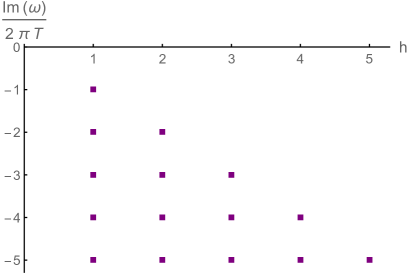
(a)

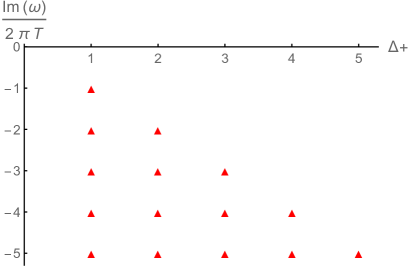
(b)

Figure 1: (a) The pole-skipping points of Majorana SYK model in space $(\mathfrak{w},h)$;  (b) The pole-skipping points of the bulk scalar field in space $(\mathfrak{w},\Delta_{+})$.

The result (62) is the same as the pole-skipping points for standard quantization (46) which we obtained in the JT gravity. The figure 1 shows a graphical comparison between the pole-skipping points given by (62) and those obtained in the JT gravity as shown in (46).

There are additional pole-skipping points in Eq. (60). The expression (60) is invariant under $h\rightarrow 1-h$ up to sign and the function $A(h)$. Note that the sign and $A(h)$ are not important for pole-skipping. Thus the additional pole-skipping points are obtained after taking replacement $h\rightarrow 1-h$ in Eq. (62). This transformation $h\rightarrow 1-h$ is similar to transformation $\Delta_{+}\rightarrow 1-\Delta_{+}$ for alternative quantization, so we define a new dimension $h_{-}=1-h$ of operators in SYK corresponding to the boundary scaling dimension $\Delta_{-}=1-\Delta_{+}$. The pole-skipping points in plane $(\mathfrak{w},h_{-})$ are

$$\begin{split}\mathfrak{w}&=-i,\quad h_{-}=0\,;\\ \mathfrak{w}&=-2i,\quad h_{-}=0,-1\,;\\ \mathfrak{w}&=-3i,\quad h_{-}=0,-1,-2\,;\\ &\qquad\qquad\vdots\end{split}$$ (63)

The result (63) is the same as the pole-skipping points for alternative quantization (48). We draw figure 2 of pole-skipping points in space $(\mathfrak{w},h_{-})$ versus pole-skipping points in space $(\mathfrak{w},\Delta_{-})$, and show that they are the same. So our assumption that $h_{-}$ corresponds to $\Delta_{-}$ is reasonable.

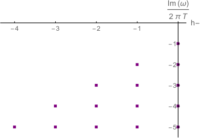
(a)

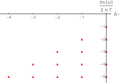
(b)

Figure 2: (a) The pole-skipping points of the Majorana SYK model in space $(\mathfrak{w},h_{-})$;  (b) The pole-skipping points of the bulk scalar field with alternative quantization in space $(\mathfrak{w},\Delta_{-})$.

3 Comparison of pole-skipping in charged JT gravity and complex SYK model

We perceive that this AdS/CFT correspondence is also applicable in the complex SYK model. We will also show this holography through the consistency of pole-skipping of Green’s function at charged JT gravity and the complex SYK model.

3.1 Pole-skipping in charged JT gravity

We will consider the pole-skipping on the boundary of the bulk theory and we will justify the reasons later. We consider the following quadratic action for the complex scalar field Thomas

$$S=-\int d^{2}x\sqrt{-g}\big{[}(D^{\mu}\Psi)^{\ast}D_{\mu}\Psi+m^{2}\Psi^{\ast}\Psi\big{]}$$ (64)

with $D_{\mu}=\partial_{\mu}-ieA_{\mu}$. The black hole solution is

$$ds^{2}=\frac{L^{2}}{u^{2}}\left(-\left(1-\frac{u^{2}}{u_{0}^{2}}\right)dt^{2}+\frac{du^{2}}{1-\frac{u^{2}}{u_{0}^{2}}}\right)$$ (65)

with

$$A=\epsilon\bigg{(}\frac{1}{u}-\frac{1}{u_{0}}\bigg{)}dt,$$ (66)

where $u_{0}$ is the horizon radius, $L$ is the curvature radius of AdS₂, and $\epsilon$ is a constant related to chemical potential. Note that we have neglected the backreaction of the gauge field on the background metric. The Hawking temperature is $T=\frac{1}{2\pi u_{0}}$. Substituting complex scalar field $\Psi(t,u)=e^{-i\omega t}\Psi(\omega,u)$ into the wave equation in the geometry (65) Faulkner

$$\partial^{2}_{u}\Psi+\frac{2u}{u^{2}-u_{0}^{2}}\partial_{u}\Psi+\bigg{(}-\frac{m^{2}L^{2}}{u^{2}-\frac{u^{4}}{u_{0}^{2}}}+\frac{\big{[}\omega+\epsilon(\frac{\alpha}{u}-\frac{\alpha}{u_{0}})\big{]}^{2}}{1-\frac{2u^{2}}{u_{0}^{2}}+\frac{u^{4}}{u_{0}^{4}}}\bigg{)}\Psi=0.$$ (67)

The parameter $\alpha$ is the coupling strength of the Maxwell field interacting with the scalar field. Considering the asymptotic behavior of $\Psi(t,u)$ as $u\rightarrow 0$, we can calculate the conformal dimension of the scalar field $\Psi(t,u)$ from Eq. (67). This is a homogeneous equation, which can be solved by a power function. Let $\Psi\sim u^{\Delta}$, in the case of the asymptotic boundary ($u\rightarrow 0$), Eq. (67) reduced to

$$\Delta(1-\Delta)+m^{2}L^{2}-\alpha^{2}\epsilon^{2}=0$$ (68)

which implies two results for $\Delta$

$$\Delta_{\pm}=\frac{1}{2}\pm\sqrt{\frac{1}{4}+m^{2}L^{2}-\alpha^{2}\epsilon^{2}}.$$ (69)

Introducing the relation

$$\Delta_{+}=\frac{1}{2}+\nu,\quad\nu=\sqrt{\frac{1}{4}+m^{2}L^{2}-\alpha^{2}\epsilon^{2}},\quad{\rm and}\;\;\Delta_{-}=\frac{1}{2}-\nu=1-\Delta_{+},$$ (70)

the asymptotic behavior of two linearly independent solutions can be obtained as

$$\Psi(u)\sim\big{(}\frac{1}{u}-\frac{1}{u_{0}}\big{)}^{-\frac{1}{2}\mp\nu}\big{(}\frac{u_{0}+u}{u_{0}-u}\big{)}^{\frac{i\omega u_{0}}{2}-i\alpha\epsilon}\,_{2}F_{1}\bigg{[}\frac{1}{2}\pm\nu+i\omega u_{0}-i\alpha\epsilon,\frac{1}{2}\pm\nu-i\alpha\epsilon,1\pm 2\nu;\frac{2u}{u-u_{0}}\bigg{]}.$$

The retarded Green’s function of $\Psi$ around the asymptotic boundary can be obtained from Eq. (3.1)

$$G_{R}(\omega)=(4\pi T)^{2\Delta_{+}-1}\frac{\Gamma(1-2\Delta_{+})\Gamma(\Delta_{+}-\frac{i\omega}{2\pi T}+i\alpha\epsilon)\Gamma(\Delta_{+}-i\alpha\epsilon)}{\Gamma(2\Delta_{+}-1)\Gamma(1-\Delta_{+}-\frac{i\omega}{2\pi T}+i\alpha\epsilon)\Gamma(1-\Delta_{+}-i\alpha\epsilon)}.$$ (72)

Here we prove that the retarded Green’s function (44) is the neutral limit of Eq. (72). We use the Legendre duplication formula $\Gamma(z)\Gamma(z+\frac{1}{2})=2^{1-2z}\pi^{1/2}\Gamma(2z)$ to make $\Gamma(\frac{1}{2}-\Delta_{+})=4^{\Delta_{+}}\pi^{1/2}\frac{\Gamma(1-2\Delta_{+})}{\Gamma(1-\Delta_{+})}$ and $\Gamma(-\frac{1}{2}+\Delta_{+})\Gamma(\Delta_{+})=2^{2-2\Delta_{+}}\pi^{1/2}\Gamma(2\Delta_{+}-1)$. The bulk retarded Green’s function (44) of the scalar field in JT gravity, obtained in subsection 2.1.2, becomes

$$G_{R} = (\pi T)^{2\Delta_{+}-1}\frac{\Gamma(\Delta_{+}-\frac{i\omega}{2\pi T})}{\Gamma(1-\Delta_{+}-\frac{i\omega}{2\pi T})}\frac{\Gamma(\frac{1}{2}-\Delta_{+})}{\Gamma(-\frac{1}{2}+\Delta_{+})}$$ (73)

$$= (\pi T)^{2\Delta_{+}-1}4^{\Delta_{+}}\sqrt{\pi}\frac{\Gamma(\Delta_{+}-\frac{i\omega}{2\pi T})\Gamma(1-2\Delta_{+})\Gamma(\Delta_{+})}{\Gamma(1-\Delta_{+}-\frac{i\omega}{2\pi T})\Gamma(1-\Delta_{+})\Gamma(-\frac{1}{2}+\Delta_{+})\Gamma(\Delta_{+})}$$

$$= (4\pi T)^{2\Delta_{+}-1}\frac{\Gamma(\Delta_{+}-\frac{i\omega}{2\pi T})\Gamma(1-2\Delta_{+})\Gamma(\Delta_{+})}{\Gamma(1-\Delta_{+}-\frac{i\omega}{2\pi T})\Gamma(1-\Delta_{+})\Gamma(2\Delta_{+}-1)}.$$

It is easy to see that the retarded Green’s function (72) will become Eq. (73) when $\alpha=0$.

Let’s now redirect our attention to the discussion of Eq. (72). We set $\alpha=1$ hereafter for simplicity, and we regard $i\big{(}\frac{\omega}{2\pi T}-\epsilon\big{)}$ as a whole term. The pole-skipping points are located in

$$\begin{split}\left(\frac{\omega}{2\pi T}-\epsilon\right)&=-i,\quad\Delta_{+}=1;\\ \left(\frac{\omega}{2\pi T}-\epsilon\right)&=-2i,\quad\Delta_{+}=1,2;\\ \left(\frac{\omega}{2\pi T}-\epsilon\right)&=-3i,\quad\Delta_{+}=1,2,3;\\ &\qquad\qquad\vdots\end{split}$$ (74)

Note that in this subsection, we have evaluated the pole-skipping points on the boundary of the bulk, unlike in the previous section where we also evaluated them near the event horizon. This is because the scalar potential vanishes at the event horizon, which makes it difficult to observe the effect of charge on the pole-skipping phenomenon. However, this approach can still capture the main physics compared to the pole-skipping points in the complex SYK model. We will see this in the next subsection.

3.2 Pole-skipping in complex SYK model

The complex SYK model describes $N\gg 1$ complex fermions with random interactions Subir ; Gu ; Maria . The Hamiltonian is Subir ; Maria

$$H=\frac{1}{2N^{3/2}}\sum^{N}_{i,j,k,l=1}J_{ij;kl}c^{\dagger}_{i}c^{\dagger}_{j}c_{k}c_{l}-\mu\sum_{i}c^{\dagger}_{i}c_{i}\,,$$ (75)

where $c_{i}$ is complex fermion obeying the anticommutation relations, and the $J_{ij;kl}$ are complex, independent Gaussian random couplings with zero mean. This system also has a conserved $U(1)$ density $\mathcal{Q}$ which is related to the average fermion number as $\mathcal{Q}=\frac{1}{N}\sum_{i}<c^{\dagger}_{i}c_{i}>$.

The conformal two-point function of the complex SYK model is given as Gu

$$G^{c}(\tau_{1},\tau_{2})=-b\frac{{\rm sgn}(\tau_{12})}{|\tau_{12}|^{2\Delta}}e^{2\pi\mathcal{E}(\frac{1}{2}-\frac{\tau}{\beta})},$$ (76)

where $\mathcal{E}$ is the dimensionless spectral asymmetry parameter which implicitly depends on chemical potential. The conformal effective action of the complex SYK model is

$$S_{\rm CFT}=-\frac{N}{2}{\rm log}\;{\rm det}(-\Sigma)-\frac{N}{2}\int d\tau_{1}d\tau_{2}\bigg{[}\Sigma(\tau_{1},\tau_{2})G(\tau_{1},\tau_{2})+\frac{1}{q}\big{(}-G(\tau_{1},\tau_{2})G(\tau_{2},\tau_{1})\big{)}^{\frac{q}{2}}\bigg{]}.$$

Similar to the Majorana SYK model, the complex SYK model can also be described as a conformal field theory perturbed by an infinite set of irrelevant primary operators. The conformal perturbation theory is still valid for the complex SYK model

$$S_{{\rm SYK}}=S_{{\rm CFT}}+\sum_{h}g_{h}\int d\tau\;\langle\mathcal{O}^{A/S}_{h}(\tau)\rangle-\frac{1}{2}\sum_{h,h^{\prime}}g_{h}g_{h^{\prime}}\int d\tau_{1}d\tau_{2}\;\langle\mathcal{O}^{A/S}_{h}(\tau_{1})\mathcal{O}^{A/S}_{h^{\prime}}(\tau_{2})\rangle+\dots..$$

The difference from Majorana SYK is that there are two kinds of bilinear primary operators, $\mathcal{O}^{A}_{h}(\tau)$ and $\mathcal{O}^{S}_{h}(\tau)$, representing particle-hole symmetry and asymmetry respectively Maria ; Gu . These two irrelevant operators can be schematically represented as $\mathcal{O}^{A}_{h_{n}}=f^{\dagger}_{i}\partial^{1+2n}_{\tau}f_{i}$ and $\mathcal{O}^{S}_{h_{n}}=f^{\dagger}_{i}\partial^{2n}_{\tau}f_{i}$ for nonnegative integer $n$ Kitaev ; Polchinski ; Maria ; Gross2 . The retarded Green’s function in frequency space can be expanded as

$$G_{R}(\omega)=G_{R}^{c}(\omega)+\delta G^{A/S}_{R}(\omega)\,.$$ (77)

Here $G_{R}^{c}(\omega)$ denotes conformal part and its expression is

$$G_{R}^{c}(\omega)=-i\frac{C}{J}\left(\frac{J}{2\pi T}\right)^{1-2\Delta}e^{-i\theta}\frac{\Gamma(\Delta-\frac{i\omega}{2\pi T}+i\mathcal{E})}{\Gamma(1-\Delta-\frac{i\omega}{2\pi T}+i\mathcal{E})}\,.$$ (78)

$\delta G^{A/S}_{R}(\omega)$ can be divided into two part as $\delta G^{A/S}_{R}(\omega)=\delta G^{A}_{R}(\omega)+\delta G^{S}_{R}(\omega)$ correspond to operators $\mathcal{O}^{A}$ and $\mathcal{O}^{S}$, where $\delta G^{A/S}_{R}(\omega)$ is

$$\begin{split}\delta G^{A/S}_{R}(\omega)\propto f^{A/S}_{R}(\omega)G_{R}^{c}(\omega)\,,\end{split}$$ (79)

and $f^{A/S}_{R}(\omega)$ is given as Maria

$$\begin{split}&f^{A}_{R}(\omega)=\frac{(2\pi)^{h-2}{\rm cos}\frac{\pi h}{2}\Gamma(h)^{2}}{{\rm cos}(\pi h)\Gamma(2h-1)}\bigg{[}\frac{\Gamma(h)}{\Gamma(1-h)}\bigg{(}e^{2i\theta}-\frac{{\rm sin}(\frac{\pi h}{2}-2\pi\Delta)}{{\rm sin}\frac{\pi h}{2}}\bigg{)}J_{h}(\omega)-(h\rightarrow 1-h)\bigg{]}\,,\\ &f^{S}_{R}(\omega)=\frac{i(2\pi)^{h-2}{\rm sin}\frac{\pi h}{2}\Gamma(h)^{2}}{{\rm cos}(\pi h)\Gamma(2h-1)}\bigg{[}\frac{\Gamma(h)}{\Gamma(1-h)}\bigg{(}\frac{{\rm cos}(\frac{\pi h}{2}-2\pi\Delta)}{{\rm cos}\frac{\pi h}{2}}-e^{2i\theta}\bigg{)}J_{h}(\omega)-(h\rightarrow 1-h)\bigg{]}\,.\end{split}$$

With substitution, one can check that $\delta G^{A/S}_{R}(\omega)$ has the following contribution

$$\delta G^{A/S}_{R}(\omega)\propto(A^{A}(h)+A^{S}(h))\bigg{[}\frac{\Gamma(1+h-\Delta-\frac{i\omega}{2\pi T}+i\mathcal{E})}{\Gamma(2+h-\Delta-\frac{i\omega}{2\pi T}+i\mathcal{E})}-(h\rightarrow 1-h)\bigg{]}\,,$$ (80)

where $A^{A/S}(h)$ is a function that depends only on $h$, and it does not affect the locations of pole-skipping. By shifting $i\big{(}\frac{\omega}{2\pi T}-\mathcal{E}\big{)}\rightarrow i\big{(}\frac{\omega}{2\pi T}-\mathcal{E}\big{)}+2$, the equation (80) becomes

$$\delta G^{A/S}_{R}(\omega)\propto(A^{A}(h)+A^{S}(h))\bigg{[}\frac{\Gamma\big{(}h-1-\Delta-i\big{(}\frac{\omega}{2\pi T}-\mathcal{E}\big{)}\big{)}}{\Gamma\big{(}h-\Delta-i\big{(}\frac{\omega}{2\pi T}-\mathcal{E}\big{)}\big{)}}-(h\rightarrow 1-h)\bigg{]}\,.$$ (81)

We can obtain the common poles and zeros of the two terms from Eq. (81):

$$\left\{\begin{aligned} &h-1-\Delta-i\big{(}\frac{\omega}{2\pi T}-\mathcal{E}\big{)}=0,-1,-2,-3,\cdots\quad{\rm and}\\ &-h-\Delta-i\big{(}\frac{\omega}{2\pi T}-\mathcal{E}\big{)}=0,-1,-2,-3,\cdots\quad\text{(lines of pole)}\,,\\ &h-\Delta-i\big{(}\frac{\omega}{2\pi T}-\mathcal{E}\big{)}=0,-1,-2,-3,\cdots\quad\quad{\rm and}\\ &1-h-\Delta-i\big{(}\frac{\omega}{2\pi T}-\mathcal{E}\big{)}=0,-1,-2,-3,\cdots\quad\text{(lines of zero)}\,.\end{aligned}\right.$$ (82)

Our interest is at the large $q$ limit, where $\Delta=1/q$ becomes 0. We can obtain a pole-skipping point in $\big{(}\frac{\omega}{2\pi T}-\mathcal{E},h\big{)}$ space by finding an intersection between a line of zeros and a line of poles in Eq. (81). The result is

$$\begin{split}\left(\frac{\omega}{2\pi T}-\mathcal{E}\right)&=-i,\quad h=1;\\ \left(\frac{\omega}{2\pi T}-\mathcal{E}\right)&=-2i,\quad h=1,2;\\ \left(\frac{\omega}{2\pi T}-\mathcal{E}\right)&=-3i,\quad h=1,2,3;\\ &\qquad\qquad\vdots\end{split}$$ (83)

If we interpret $\mathcal{E}$ as $\epsilon$ in (74), the result Eq. (83) is the same as the result in charged JT gravity Eq. (74).

In order to compare $\epsilon$ to $\mathcal{E}$, we need to discuss thermodynamics in charged JT gravity and the complex SYK model. For the thermodynamics of charged black holes in the structure of AdS₂ metric

$$ds^{2}=(dr^{2}-dt^{2})/r^{2},$$ (84)

with gauge field $A=(\epsilon/r)dt$. The Bekenstein-Hawking entropy density $\mathcal{S}_{BH}$ at $T=0$ has a relation Sen1 ; Sen2

$$\frac{\partial\mathcal{S}_{BH}}{\partial\mathcal{Q}}=2\pi\epsilon,$$ (85)

where $\mathcal{Q}$ is a conserved $U(1)$ charge density. As the charge $\mathcal{Q}$ increases, the horizon moves closer to the boundary, and its area $\mathcal{A}_{h}$ increases. In black hole thermodynamics, the Bekenstein-Hawking entropy density $\mathcal{S}_{BH}$ is related to the area of the horizon via $\mathcal{S}_{BH}=\mathcal{A}_{h}/(4G_{N}\mathcal{A}_{b})$, where $G_{N}$ is Newton’s constant Subir .

In the complex SYK model, the computation of the statistical zero-temperature entropy density $\mathcal{S}$ follows Parcollet ; Georges and relies on the thermodynamic Maxwell relation:

$$\bigg{(}\frac{\partial\mathcal{S}}{\partial\mathcal{Q}}\bigg{)}_{T}=-\bigg{(}\frac{\partial\mu}{\partial T}\bigg{)}_{\mathcal{Q}}\,.$$ (86)

At the $T\rightarrow 0$ limit, $\big{(}\frac{\partial\mu}{\partial T}\big{)}_{\mathcal{Q}}=-2\pi\mathcal{E}$. Then the Maxwell relation in Eq. (86) leads to

$$\bigg{(}\frac{\partial\mathcal{S}}{\partial\mathcal{Q}}\bigg{)}=2\pi\mathcal{E}\,.$$ (87)

The form (87) in the complex SYK model is the same as Eq. (85) in charged JT gravity. From this comparison, we can interpret the parameter $\epsilon$ as the spectral asymmetry parameter $\mathcal{E}$.

Hence the pole-skipping points (74) and (83) show good agreement with each other. Compared to the pole-skipping points in the Majorana SYK model (62), in the complex SYK model, the spectral asymmetry shifts the pole-skipping frequencies amount of $-\mathcal{E}$.

In the complex SYK model, we can still define a variable $h_{-}$ corresponding to $\Delta_{-}$ in charged JT gravity. Because this relationship is the same as that obtained in the previous section, we do not repeat it here.

4 Discussion and Conclusion

In summary, we study the pole-skipping phenomenon on both $(1+1)$-dimensional bulk theories and $(0+1)$-dimensional quantum field theories. We have found a connection between the pole-skipping of gravity and the field theory. In contrast to higher dimensional theories, there is no momentum $k$ degrees of freedom in $(1+1)$-dimensional bulk theories. Instead, we treat mass $m$ as a substitute for momentum for the purpose of identifying the pole-skipping points. Hence our resulting pole-skipping points live in $(\omega,m)$ space instead of $(\omega,k)$ space.

For the JT gravity, we study pole-skipping points by analyzing the near horizon and computing the exact retarded Green’s function. We compare the pole-skipping points in the neutral JT gravity with those in the Majorana SYK model, thanks to the well-known result of the two-point function in the SYK models. The pole-skipping points in space $(\mathfrak{w},h)$ in the Majorana SYK model match those by computing the holographic retarded Green’s function in space $(\mathfrak{w},\Delta_{+})$ in JT gravity with standard quantization. Moreover, the pole-skipping points in space $(\mathfrak{w},h_{-})$ in the Majorana SYK model match those in space $(\mathfrak{w},\Delta_{-})$ in JT gravity with alternative quantization.

Finally, we compute the pole-skipping points in charged JT gravity and in the complex SYK model. The pole-skipping points in these two systems are also in one-to-one correspondence. Compared to the Majorana SYK model, the pole-skipping frequencies are shifted by the spectral asymmetry parameter $\mathcal{E}$, which is analogous to $\epsilon$ with respect to chemical potential in the charged JT gravity. By analyzing zero temperature thermodynamics in charged JT gravity and complex SYK model, we further provide evidence that $\epsilon$ and $\mathcal{E}$ play the same role in each theory.

It would be interesting to study further the pole-skipping of the charged JT gravity and the complex SYK model. The fact that the pole-skipping frequency could be shifted by $\epsilon$ and $\mathcal{E}$ in each model contradicts the well-known result about pole-skipping. As we have just mentioned, the existence of the pole-skipping points in space $(\omega,m)$ instead of space $(\omega,k)$ is a unique property of the phenomenon in two-dimensional gravity. Therefore, we perceive that this type of shift is also a unique property of the pole-skipping phenomenon in charged two-dimensional gravity.

Appendix A Details of near-horizon expansions

In this appendix, we show the details of the near-horizon expansions of the equations of motion. We can calculate a Taylor series solution to the equation of motion for the scalar mode $\Psi(r)$ when the matrix equation (10) is satisfied. The first few elements of the matrix are shown below

$$M_{11}=-\frac{m^{2}}{2};$$

$$M_{21}=0,\quad M_{22}=\frac{f^{\prime\prime}(r_{h})-m^{2}}{4};$$

$$M_{31}=0,\quad M_{32}=\frac{f^{(3)}(r_{h})}{12},\quad M_{33}=\frac{m^{2}-3f^{\prime\prime}(r_{h})}{6r_{h}};$$ (88)

$$M_{41}=0,\quad M_{42}=\frac{f^{(4)}(r_{h})}{48},\quad M_{43}=\frac{f^{(3)}(r_{h})}{6},\quad M_{43}=\frac{6f^{\prime\prime}(r_{h})-m^{2}}{8};$$

$$M_{51}=0,\quad M_{52}=\frac{f^{(5)}(r_{h})}{240},\quad M_{53}=\frac{f^{(4)}(r_{h})}{24},\quad M_{54}=\frac{f^{(3)}(r_{h})}{4},\quad M_{54}=\frac{10f^{\prime\prime}(r_{h})-m^{2}}{10}.$$

Appendix B Pole-skipping of Dirac field in JT gravity

As a way to confirm the validity of our holographic computation method, we consider the Dirac field (spin $s=\frac{1}{2}$) in the same background (9). The Dirac equation is given as

$$(\Gamma^{M}D_{M}-m)\psi_{\pm}=0.$$ (89)

The capital letter $M$ denotes the indices of bulk spacetime coordinates and small letters $a,b$ denote tangent space indices. The covariant derivative of bulk spacetime acting on fermions is defined by $D_{M}=\partial_{M}+\frac{1}{4}(\omega_{ab})_{M}\Gamma^{ab}$, where $\Gamma_{ab}\equiv\frac{1}{2}[\Gamma_{a},\Gamma_{b}]$. $\Gamma_{a}$ are Gamma matrices which satisfy Grassman algebra $\{\Gamma^{a},\Gamma^{b}\}=2\eta^{ab}$ N1 ; Cai . The spinors are two dimensional $\psi_{\pm}(r,t)=e^{-i\omega t}\left(\begin{array}[]{c}\psi_{+}(r)\\ \psi_{-}(r)\\ \end{array}\right)$ and we use the following gamma matrices representation Wilczek

$$\Gamma^{\underline{v}}=i\sigma^{2},\quad\Gamma^{\underline{r}}=\sigma^{3}.$$ (90)

We choose the orthonormal frame to be

$$E^{\underline{v}}=\frac{1+f(r)}{2}dv-dr,\quad E^{\underline{r}}=\frac{1-f(r)}{2}dv+dr,$$ (91)

for which

$$ds^{2}=\eta_{ab}E^{a}E^{b},\quad\eta_{ab}={\rm diag}(-1,1).$$ (92)

The spin connections for this frame are given by

$$\omega_{\underline{rr}}=0,\quad\omega_{\underline{vr}}=-\frac{f^{\prime}(r)}{2}.$$ (93)

Using these spin connections (93) and the Eddington-Finkelstein coordinate (9) of Schwarzschild-AdS₂

$$ds^{2}=-f(r)dv^{2}+2dvdr,$$ (94)

one can calculate the Dirac equation to be

$$\left\{\begin{aligned} &\big{(}f^{\prime}(r)-4(m+i\omega)\big{)}\psi_{+}(r)+\big{(}f^{\prime}(r)-4i\omega\big{)}\psi_{-}(r)+2\big{(}f(r)-1\big{)}\psi^{\prime}_{-}(r)\\ &+2\big{(}f(r)+1\big{)}\psi^{\prime}_{+}(r)=0,\\ &\big{(}4i\omega-f^{\prime}(r)\big{)}\psi_{+}(r)-\big{(}4m+f^{\prime}(r)-4i\omega\big{)}\psi_{-}(r)-2\big{(}f(r)+1\big{)}\psi^{\prime}_{-}(r)\\ &+2\big{(}f(r)-1\big{)}\psi^{\prime}_{+}(r)=0.\end{aligned}\right.$$ (95)

B.1 Pole-skipping: near-horizon analysis

We combine the two equations of (95) and expand them near the horizon $r_{h}$. The first-order equation near the horizon is

$$1st:\quad(2\pi T-2i\omega-m)\psi_{+}+(2\pi T-2i\omega+m)\psi_{-}=0.$$ (96)

We take the value of coefficients $(2\pi T-2i\omega-m)$ and $(2\pi T-2i\omega+m)$ to be 0 and thus there are two independent free parameters $\psi_{+}$ and $\psi_{-}$ to this equation. The first-order pole-skipping point is obtained as

$$\mathfrak{w}=-\frac{i}{2},\quad\mathfrak{m}=0,\quad\Delta=\frac{1}{2}.$$ (97)

We expand the Dirac equation in higher order

$$2nd: \bigg{(}\frac{m(\pi T-m)-\frac{m^{2}}{4\pi T}}{m+2\pi T-2i\omega}\bigg{)}\psi^{0}_{+}+\frac{1}{2}\bigg{(}3-\frac{i\omega}{\pi T}\bigg{)}\psi^{1}_{+}=0,$$ (98)

$$3rd: \frac{m(4\pi^{2}T^{2}-m^{2})(m^{2}+10m\pi T-16\pi^{2}T^{2}-2im\omega)}{8\pi T(3\pi T-i\omega)(m+2\pi T-2i\omega)}\psi^{0}_{+}+\big{(}5-\frac{i\omega}{\pi T}\big{)}\psi^{2}_{+}=0,$$ (99)

$$4th: \frac{m(20m^{2}\pi^{2}T^{2}-64\pi^{4}T^{4}-m^{4})(m^{2}+14m\pi T-36\pi^{2}T^{2}-2im\omega)}{32\pi T(3\pi T-i\omega)(5\pi T-i\omega)(m+2\pi T-2i\omega)}\psi^{0}_{+}$$ (100)

$$+\frac{3}{2}\big{(}7-\frac{i\omega}{\pi T}\big{)}\psi^{3}_{+}=0,$$

$$5th: \frac{m(56m^{4}\pi^{2}T^{2}+2304\pi^{6}T^{6}-784m^{2}\pi^{4}T^{4}-m^{6})(m^{2}+18m\pi T-64\pi^{2}T^{2}-2im\omega)}{192\pi T(3\pi T-i\omega)(5\pi T-i\omega)(7\pi T-i\omega)(m+2\pi T-2i\omega)}\psi^{0}_{+}$$ (101)

$$+2\big{(}9-\frac{i\omega}{\pi T}\big{)}\psi^{4}_{+}=0.$$

In general bulk dimensions, the mass $m$ of the fermionic field and the scaling dimension $\Delta$ of the dual operator are related via

$$\Delta=\frac{d+1}{2}+m.$$ (102)

In the case of AdS₂, $d=1$, and we get the relation $\Delta=\frac{1}{2}+m$. The higher-order pole-skipping points are

$$\begin{split}\mathfrak{w}&=-\frac{3i}{2},\quad\mathfrak{m}=-1,0,1,\quad\Delta=-\frac{1}{2},\frac{1}{2},\frac{3}{2}\,;\\ \mathfrak{w}&=-\frac{5i}{2},\quad\mathfrak{m}=-2,-1,0,1,2,\quad\Delta=-\frac{3}{2},-\frac{1}{2},\frac{1}{2},\frac{3}{2},\frac{5}{2}\,;\\ \mathfrak{w}&=-\frac{7i}{2},\quad\mathfrak{m}=-3,-2,-1,0,1,2,3,\quad\Delta=-\frac{5}{2},-\frac{3}{2},-\frac{1}{2},\frac{1}{2},\frac{3}{2},\frac{5}{2},\frac{7}{2}\,;\\ &\qquad\qquad\vdots\end{split}$$ (103)

We calculate the first few order pole-skipping points and plot them in figure 3.

B.2 Pole-skipping from Green’s function

In this subsection, we also compute the pole-skipping points from the exact retarded Green’s function on the boundary. We substitute the metric (36) into the Dirac equation (89)

$$\left\{\begin{aligned} -2iL\omega{\rm Csch}(u)\psi_{-}(u)+({\rm Coth}(u)-2Lm)\psi_{+}(u)+2\psi^{\prime}_{+}(u)=0,\\ (2Lm+{\rm Coth}(u))\psi_{-}(u)-2iL\omega{\rm Csch}(u)\psi_{+}(u)+2\psi^{\prime}_{-}(u)=0.\end{aligned}\right.$$ (104)

Combining the two equations of (104), we obtain

$$\left\{\begin{aligned} &4\psi^{\prime\prime}_{+}(u)+8{\rm Coth}(u)\psi^{\prime}_{+}(u)\\ &+\big{(}3{\rm Coth}^{2}(u)-4mL{\rm Coth}(u)+2(\omega^{2}L^{2}-1){\rm Csch}^{2}(u)-4m^{2}L^{2}\big{)}\psi_{+}(u)=0,\\ &4\psi^{\prime\prime}_{-}(u)+8{\rm Coth}(u)\psi^{\prime}_{-}(u)\\ &+\big{(}3{\rm Coth}^{2}(u)+4mL{\rm Coth}(u)+2(\omega^{2}L^{2}-1){\rm Csch}^{2}(u)-4m^{2}L^{2}\big{)}\psi_{-}(u)=0.\end{aligned}\right.$$ (105)

We do another change of variable $z={\rm tanh}^{2}(u)$, and solve these two second order differential equations (105). Near the asymptotic boundary ($z\rightarrow 1$), the two spinor components behave as

$$\psi_{+} \sim C_{1}\,{}_{2}F_{1}\bigg{[}-iL\omega,\frac{1}{2}+Lm-i\omega,1-2iL\omega;\frac{2z}{z-1}\bigg{]}$$ (106)

$$+(-2)^{2iL\omega}(\frac{z}{z-1})^{2iL\omega}C_{2}\,{}_{2}F_{1}\bigg{[}iL\omega,\frac{1}{2}+Lm+i\omega,1+2iL\omega;\frac{2z}{z-1}\bigg{]}$$

$$\sim (1-z)^{\frac{1}{4}-\frac{mL}{2}}A+(1-z)^{\frac{3}{4}+\frac{mL}{2}}B$$

$$= (1-z)^{\frac{1}{2}-\frac{\Delta}{2}}A+(1-z)^{\frac{1}{2}+\frac{\Delta}{2}}B;$$

$$\psi_{-} \sim C_{1}\,{}_{2}F_{1}\bigg{[}-iL\omega,\frac{1}{2}-Lm-i\omega,1-2iL\omega;\frac{2z}{z-1}\bigg{]}$$ (107)

$$+(-2)^{2iL\omega}(\frac{z}{z-1})^{2iL\omega}C_{2}\,{}_{2}F_{1}\bigg{[}\frac{1}{2}-Lm+i\omega,iL\omega,1+2iL\omega;\frac{2z}{z-1}\bigg{]}$$

$$\sim (1-z)^{\frac{1}{4}+\frac{mL}{2}}C+(1-z)^{\frac{3}{4}-\frac{mL}{2}}D$$

$$= (1-z)^{\frac{\Delta}{2}}C+(1-z)^{1-\frac{\Delta}{2}}D.$$

We choose $A$ as the source and the expectation value as $C$. The retarded Green’s function in this case is given by their ratio

$$G_{R}\propto i\frac{C}{A}=i\frac{\Gamma(\frac{1}{2}+Lm-i\omega L)\Gamma(\frac{1}{2}-Lm)}{\Gamma(\frac{1}{2}-Lm-i\omega L)\Gamma(\frac{1}{2}+Lm)}=i\frac{\Gamma(\Delta-i\omega L)}{\Gamma(1-\Delta-i\omega L)}\frac{\Gamma(1-\Delta)}{\Gamma(\Delta)}.$$ (108)

The poles and zeros of the Green’s function are

$$\left\{\begin{aligned} \frac{1}{2}+Lm-i\omega L=0,-1,-2,-3,\cdots\,,\qquad\text{(lines of pole)}\,,\\ \frac{1}{2}-Lm-i\omega L=0,-1,-2,-3,\cdots\,,\qquad\text{(lines of zero)}\,.\end{aligned}\right.$$ (109)

According to these two equations, we obtain the pole-skipping points

$$\begin{split}\mathfrak{w}&=-\frac{i}{2},\quad\Delta=\frac{1}{2}\,;\\ \mathfrak{w}&=-\frac{3i}{2},\quad\Delta=-\frac{1}{2},\frac{1}{2},\frac{3}{2}\,;\\ \mathfrak{w}&=-\frac{5i}{2},\quad\Delta=-\frac{3}{2},-\frac{1}{2},\frac{1}{2},\frac{3}{2},\frac{5}{2}\,;\\ &\qquad\qquad\vdots\end{split}$$ (110)

From result (110), we can see that the pole-skipping points from the exact retarded Green’s function on the boundary are the same as these special points in (97) and (103) near the horizon. The comparison of the pole-skipping points obtained by these two methods is shown in figure 3.

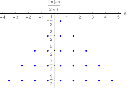
(a)

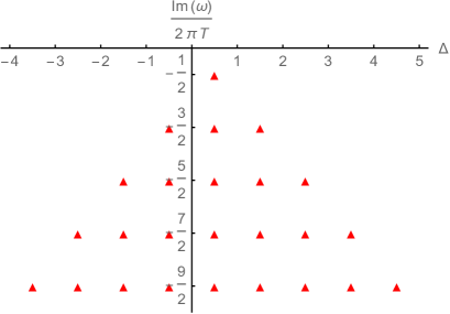
(b)

Figure 3: The pole-skipping points (103) and (110) of Dirac field in JT black hole background.  (a) From near the horizon ;  (b) From boundary retarded Green’s function.

References

- (1) J. Maldacena, The Large-N Limit of Superconformal Field Theories and Supergravity, Int. J. Theor. Phys. 38 (1999) 1113, arXiv:9711200.
- (2) E. Witten, Anti-de Sitter space and holography, Adv. Theor. Math. Phys. 2 (1988) 253, arXiv:9802150.
- (3) E. Witten, Anti-de Sitter space, thermal phase transition, and confinement in gauge theories, Adv. Theor. Math. Phys. 2 (1998) 505, arXiv:9803131.
- (4) S. S. Gubser, I. R. Klebanov and A. M. Polyakov, Gauge theory correlators from noncritical string theory, Phys. Lett. B. 428 (1998) 105, arXiv:9802109.
- (5) J. Casalderrey-Solana, H. Liu, D. Mateos, K. Rajagopal and U. A. Wiedemann, Gauge/String Duality, Hot QCD and Heavy Ion Collisions, Cambridge Univ. Press (2014), arXiv:1101.0618.
- (6) M. Natsuume, AdS/CFT Duality User Guide, Springer Japan, Tokyo (2015), arXiv:1409.3575.
- (7) M. Ammon and J. Erdmenger, Gauge/gravity duality: Foundations and applications, Cambridge Univ. Press (2015).
- (8) J. Zaanen, Y. W. Sun, Y. Liu and K. Schalm, Holographic Duality in Condensed Matter Physics, Cambridge Univ. Press (2015).
- (9) S. A. Hartnoll, A. Lucas and S. Sachdev, Holographic quantum matter, The MIT Press (2018).
- (10) S. Grozdanov, K. Schalm, and V. Scopelliti, Black Hole Scrambling from Hydrodynamics, Phys. Rev. Lett. 120, 231601 (2018), arXiv:1710.00921.
- (11) M. Blake, R. A. Davions, S. Grozdanov, and H. Liu, Many-body chaos and energy dynamics in holography, JHEP 2018, 35 (2018), arXiv:1809.01169.
- (12) S. Grozdanov, On the connection between hydrodynamics and quantum chaos in holographic theories with stringy corrections, JHEP 2019, 48 (2019), arXiv:1811.09641.
- (13) M. Natsuume and T. Okamura, Holographic chaos, pole-skipping, and regularity, Progress of Theoretical and Experimental Physics, 1 (2020) 013B07, arXiv:1905.12014.
- (14) M. Natsuume and T. Okamura, Nonuniqueness of Green’s functions at special points, arXiv:1905.12015.
- (15) M. Blake, R. A. Davison, and D. Vegh, Horizon constraints on holographic Green’s functions, JHEP 2020, 77 (2020), arXiv:1904.12883.
- (16) S. Das, B. Ezhuthachan and A. Kundu, Real time dynamics from low point correlators in 2d BCFT, JHEP 2019 141 (2019), arXiv:1907.08763.
- (17) N. Abbasi and S. Tahery, Complexified quasinormal modes and the pole-skipping in a holographic system at finite chemical potential, JHEP 2020 76 (2020), arXiv:2007.10024.
- (18) N. Abbasi and J. Tabatabaei, Quantum chaos, pole-skipping and hydrodynamics in a holographic system with chiral anomaly, JHEP 2020, 50 (2020), arXiv:1910.13696.
- (19) C. Choi, M. Mezei and G. Sárosi, Pole skipping away from maximal chaos, JHEP 2021, 207 (2021), arXiv: 2010.08558.
- (20) K. Sil, Pole skipping and chaos in anisotropic plasma: a holographic study, JHEP 2021, 232 (2021), arXiv:2012.07710.
- (21) Y. Ahn, V. Jahnke, H. S. Jeong, K. Y. Kim, K. S. Lee, and M. Nishida, Classifying pole-skipping points, arXiv:2010.16166.
- (22) M. Atashi and K. Bitaghsir Fadafan, Holographic pole-skipping of flavor branes, Journal of Holography Applications in Physics, 2(2), pp. 39-46 (2022). doi: 10.22128/jhap.2022.519.1020.
- (23) M. Natsuume and T. Okamura, Pole-skipping with finite-coupling corrections, Phys. Rev. D 100, 126012 (2019), arXiv:1909.09168.
- (24) N. Ćeplak, K. Ramdial, and D. Vegh, Fermionic pole-skipping in holography, JHEP 2020, 203 (2020), arXiv:1910.02975.
- (25) H. Yuan, X. H. Ge, Pole-skipping and hydrodynamic analysis in Lifshitz, AdS2 and Rindler geometries, JHEP 2021, 165 (2021), arXiv:2012.15396.
- (26) N. Ćeplak and D. Vegh, Pole skipping and Rarita-Schwinger fields, Phys. Rev. D 103, 106009 (2021), arXiv:2101.01490.
- (27) H. Yuan, X. H. Ge, Analogue of the pole-skipping phenomenon in acoustic black holes, Eur. Phys. J. C 82, 167 (2022), arXiv:2110.08074.
- (28) D. Wang and Z. Y. Wang, Pole Skipping in Holographic Theories with Bosonic Fields, Phys. Rev. Lett. 129, 231603 (2022), arXiv:2208.01047.
- (29) M. Blake, H. Lee, and H. Liu, A quantum hydrodynamical description for scrambling and many-body chaos, JHEP 2018 127 (2018), arXiv:1801.00010.
- (30) H. S. Jeong, K. Y. Kim, and Y. W. Sun, Bound of diffusion constants from pole-skipping points: spontaneous symmetry breaking and magnetic field, JHEP 2021, 105 (2021), arXiv:2104.13084.
- (31) R. Jackiw, Lower dimensional gravity, Nucl. Phys. B 252, 343 (1985).
- (32) C. Teitelboim, Gravitation and Hamiltonian structure in two space-time dimensions, Phys. Lett. B 126, 41 (1983).
- (33) S. Sachdev and J. Ye, Gapless spin-fluid ground state in a random quantum Heisenberg magnet, Physical Review Letters 70 3339 (1993), arXiv:cond-mat/9212030.
-
(34)
A. Kitaev, A simple model of quantum holography,
http://online.kitp.ucsb.edu/online/entangled15/kitaev/,
http://online.kitp.ucsb.edu/online/entangled15/kitaev2/. Talks at KITP, April 7, 2015 and May 27, 2015. - (35) K. Jensen, Chaos in AdS2 holography, Phys. Rev. Lett. 117 111601 (2016), arXiv:1605.06098.
- (36) J. Maldacena, S. H. Shenker and D. Stanford, A bound on chaos, JHEP 08, 106 (2016), arXiv:1503.01409.
- (37) J. Maldacena, D. Stanford and Z. Yang, Conformal symmetry and its breaking in two dimensional Nearly Anti-de-Sitter space, PTEP 2016, no. 12, 12C104 (2016), arXiv:1606.01857.
- (38) G. Śarosi, AdS2 holography and the SYK model, arXiv:1711.08482.
- (39) J. Maldacena and D. Stanford, Remarks on the Sachdev-Ye-Kitaev model, Phys. Rev. D 94, 106002 (2016), arXiv:1604.07818.
- (40) J. Polchinski and V. Rosenhaus, The Spectrum in the Sachdev-Ye-Kitaev Model, JHEP 1604, 001 (2016), arXiv:1601.06768.
- (41) S. Cao, Y. C. Rui and X. H. Ge, Thermodynamic phase structure of complex Sachdev-Ye-Kitaev model and charged black hole in deformed JT gravity, arXiv:2103.16270.
- (42) J. Louw and S. Kehrein, The shared universality of charged black holes and the many many-body SYK model, arXiv: 2204.09629.
- (43) V. Godet and C. Marteau, New boundary conditions for , arXiv:2005.08999.
- (44) Y. Ahn, V. Jahnke, H. S. Jeong, K. Y. Kim, K. S. Lee, and M. Nishida,Pole-skipping of scalar and vector fields in hyperbolic space: conformal blocks and holography, JHEP 09, 111 (2020), arXiv:2006.00974.
- (45) D. Louis-Martinez and G. Kunstatter, On Birckhoff’s theorem in 2-D dilaton gravity, Phys. Rev. D 49, 5227 (1994).
- (46) A. Achucarro and M. E. Ortiz, Relating black holes in two-dimensions and three-dimensions, Phys. Rev. D 48, 3600 (1993), arXiv:hep-th/9304068.
- (47) J. Gegenberg, G. Kunstatter, and D. Louis-Martinez, Observables for two-dimensional black holes, Phys. Rev. D 51, 1781 (1995), arXiv:gr-qc/9408015.
- (48) D. J. Gross and V. Rosenhaus, A generalization of Sachdev-Ye-Kitaev, J. High Energ. Phys. 2017, 93 (2017), arXiv:1610.01569.
- (49) A. Kitaev and S.J. Suh, The soft mode in the Sachdev-Ye-Kitaev model and its gravity dual, J. High Energ. Phys. 2018, 183 (2018), arXiv:1711.08467.
- (50) V. Rosenhaus, An introduction to the SYK model, J. Phys. A: Math. Theor. 52 323001 (2019), arXiv:1807.03334.
- (51) M. Tikhanovskaya, H. Guo, S. Sachdev, and G. Tarnopolsky, Excitation spectra of quantum matter without quasiparticles. I. Sachdev-Ye-Kitaev models, Phys. Rev. B 103, 075141 (2021), arXiv:2010.09742.
- (52) D. J. Gross and V. Rosenhaus, A line of CFTs: from generalized free fields to SYK, J. High Energ. Phys. 2017, 86 (2017), arXiv:1706.07015.
- (53) D. J. Gross and V. Rosenhaus, All point correlation functions in SYK, J. High Energ. Phys. 2017, 148 (2017), arXiv:1710.08113.
- (54) T. Faulkner, H. Liu, J. McGreevy, and D. Vegh, Emergent quantum criticality, Fermi surfaces, and AdS2, Phys. Rev. D 83, 125002, arXiv:0907.2694.
- (55) T. Faulkner, N. Iqbal, H. Liu, J. McGreevy, and D. Vegh, Holographic non-Fermi-liquid fixed points, Phil. Trans. R. Soc. A 369, 1640 (2011), arXiv:1101.0597.
- (56) Y. Gu, A. Kitaev, S. Sachdev, and G. Tarnopolsky, Notes on the complex Sachdev-Ye-Kitaev model, JHEP 2020, 157 (2020), arXiv:1910.14099.
- (57) S. Sachdev, Bekenstein-Hawking Entropy and Strange Metals, Phys. Rev. X 5, 041025 (2015), arXiv:1506.05111.
- (58) A. Sen, Black Hole Entropy Function and the Attractor Mechanism in Higher Derivative Gravity, JHEP 09 038 (2005), arXiv:hep-th/0506177.
- (59) A. Sen, Entropy Function and AdS(2)/CFT(1) Correspondence, JHEP 11 075 (2008), arXiv:0805.0095.
- (60) O. Parcollet, A. Georges, G. Kotliar, and A. Sengupta, Overscreened Multichannel SU(N) Kondo Model: Large-N Solution and Conformal Field Theory, Phys. Rev. B 58, 3794 (1998), arXiv:cond-mat/9711192.
- (61) A. Georges, O. Parcollet, and S. Sachdev, Quantum Fluctuations of a Nearly Critical Heisenberg Spin Glass, Phys. Rev. B 63, 134406 (2001), arXiv:cond-mat/0009388.
- (62) R. G. Cai, Y. H. Qi, Y. L. Wu, and Y. L. Zhang, Topological non-Fermi liquid, Phys. Rev. D 95, 124026 (2017), arXiv:1601.03865.
- (63) F. Wilczek and A. Zee, Families from spinors, Phys. Rev. D 25, 553 (1982).