Emulating two qubits with a four-level transmon qudit
for variational quantum algorithms

Abstract

Using quantum systems with more than two levels, or qudits, can scale the computation space of quantum processors more efficiently than using qubits, which may offer an easier physical implementation for larger Hilbert spaces. However, individual qudits may exhibit larger noise, and algorithms designed for qubits require to be recompiled to qudit algorithms for execution. In this work, we implemented a two-qubit emulator using a 4-level superconducting transmon qudit for variational quantum algorithm applications and analyzed its noise model. The major source of error for the variational algorithm was readout misclassification error and amplitude damping. To improve the accuracy of the results, we applied error-mitigation techniques to reduce the effects of the misclassification and qudit decay event. The final predicted energy value is within the range of chemical accuracy. Our work demonstrates that qudits are a practical alternative to qubits for variational algorithms.

Quantum computing is widely considered a promising computing model due to its exponentially large Hilbert space Nielsen and Chuang (2000). Most current quantum processors use two-level quantum systems, or qubits, as the basic building block, inheriting from the successful experience with binary classical computers. For a qubit processor made of $N$ elementary building blocks, the size of the Hilbert space is $2^{N}$. Current research focuses on scaling up the number of qubits $N$, but this approach faces challenges such as wiring TAMATE et al. (2022), expensive control electronics Stefanazzi et al. (2022), and frequency crowding Theis et al. (2016); Schutjens et al. (2013). A complementary strategy is to increase the size of each building block by replacing the qubit with a qudit (d-level system), which yields a Hilbert space of size $d^{N}$.

The experimental use of qudits as the fundamental building blocks for quantum processors has been investigated in various systems, including photonic systems Slussarenko and Pryde (2019); Fickler et al. (2012); Malik et al. (2016); Wang et al. (2018); Lu et al. (2020); Kues et al. (2017), ion traps Bruzewicz et al. (2019); Ringbauer et al. (2022), Nuclear magnetic resonance Vandersypen and Chuang (2004); Jones (2011); Dogra et al. (2014, 2015, 2016); Gedik et al. (2015). Superconducting circuits, which are among the leading platforms for quantum computing, have also been explored for this purpose Krantz et al. (2019); Wallquist et al. (2009). The transmon is the most widely used building block in superconducting quantum processors Koch et al. (2007), and it has more than two energy levels that can potentially be utilized for computation. However, these higher levels are more susceptible to charge noise and spontaneous decay, which presents a significant challenge Peterer et al. (2015); Bianchetti et al. (2010); Dong et al. (2022). In recent years, transmons has been used as qutrits (three-level systems) in several research, including the simulation of topological Maxwell metal bands Tan et al. (2018), the dynamics of quantum information in strongly interacting systems Blok et al. (2021), and the simulation of Tensor Monopoles Tan et al. (2021). While these works using transmons were up to three levels of computational space, the results already demonstrate the potential of using transmons qudits as the fundamental building blocks for quantum processors.

Another challenge for qudit-based quantum processors is that algorithms designed for qubit-based systems must be modified and adapted to fully exploit the increased Hilbert space provided by qudits. The algorithms must be compiled using a qudit gate set, which differs from the qubit gate set Wang et al. (2020); Luo and Wang (2014); Brylinski and Brylinski (2001); Di and Wei (2011). Some well-known quantum algorithms, such as the Deutsch-Jozsa algorithm Fan (2007); Mogos (2007), Bernstein-Vazirani algorithm Krishna et al. (2016), Grover’s algorithm Ivanov et al. (2012), Quantum Fourier Transform Cao et al. (2011); Pavlidis and Floratos (2021), and Shor’s algorithm Bocharov et al. (2017), have direct generalizations of the qubit counterparts, which maintain the same principles but change the positional notation from the base-2 numeral system to the base-$d$ numeral system. However, it is challenging to directly generalize an arbitrary quantum algorithm into a qudit version simply by changing the positional notation. Certain applications, such as near-term applications, are specifically designed to run on qubit-based quantum processors Cerezo et al. (2021); Tilly et al. (2021). For example, variational quantum algorithms for chemistry applications decompose the molecule Hamiltonian into a sum of tensor products of qubit Pauli operators. However, generalizing these variational algorithms to work with qudits requires an innovative encoding mechanism. Therefore, emulating a qubit system with qudits can be a useful approach to implementing these algorithms. When the Hilbert space of a qudit is equivalent to that of an $N$-qubit system ( $2^{N}=d$), the qudit can be used to emulate the $N$-qubit system directly. For example, a qudit with $d=4$ can be used to emulate a two-qubit system, as proposed in Kiktenko et al. (2015); Dong et al. (2021).

In this paper, we present an implementation of a two-qubit emulator on a high-coherence transmon. Our transmon is designed to have the optimal operating parameters as a ququart (qudit with d=4), and it is tuned to have single-shot readout capabilities that can distinguish the lowest four levels. To create the emulator, we compiled two-qubit operations into sequences of 4-level intrinsic operations that include only neighbouring transitions and virtual-Z gates. We characterized the performance of both the intrinsic and emulated gates using randomized benchmarking and gate-set tomography. We also implemented active reset on qudit to prepare a high-fidelity initial state. We demonstrated the efficacy of a two-qubit variational quantum eigensolver algorithm on the emulator. We also analyzed the primary sources of error and implemented error mitigation techniques to obtain more accurate results.

Results

Implementation of the emulator

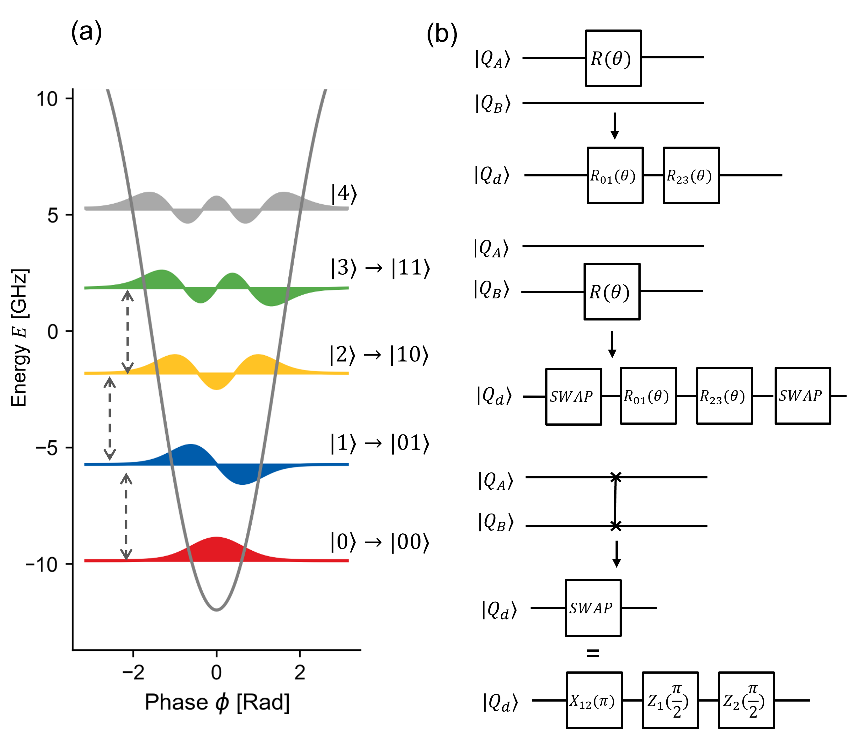
Figure 1: (a) The lowest four levels of the transmon are used as a qudit for quantum information processing. (b) The two-qubit operations are mapped to sequences of single qudit operations

[]
[]

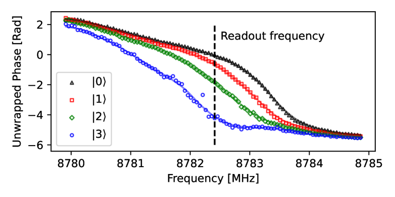
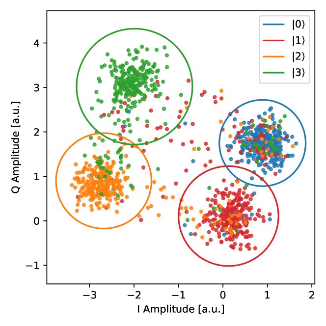
Figure 2: (a) The phase response of a resonator spectroscopy experiment is shown, where the response of the resonator was measured while the transmon was excited to the $\ket{0}$, $\ket{1}$, $\ket{2}$, and $\ket{3}$ states, respectively. (b) is the IQ plane of the single-shot readout. The states were prepared in the $\ket{0}$, $\ket{1}$, $\ket{2}$, and $\ket{3}$ states, respectively, denoted by the color. The four different levels were classified by a spherical Gaussian mixture model, where the cross denotes the center of the Gaussian distribution, and the radius of the circle denotes three times the standard deviation.

The two-qubit emulator is built using a single transmon with a coaxial geometry and off-chip packaging Spring et al. (2022); Rahamim et al. (2017), where the lowest 4 quantum states of the transmon are used as the computation space. The device has also been previously used as a qutrit Cao et al. (2022). The two-qubit emulator maps the physical states $\ket{0}$, $\ket{1}$, $\ket{2}$, $\ket{3}$ of the transmon to the $\ket{00}$, $\ket{01}$, $\ket{10}$, $\ket{11}$ states of a virtual two-qubit device. Single qubit gates for the first virtual qubit $Q_{A}$ are performed by driving transitions in the ${\ket{0},\ket{1}}$ and ${\ket{2},\ket{3}}$ subspaces in sequence. The single qubit operation on $Q_{B}$ could be implemented with a similar approach as for $Q_{A}$ by driving the two-photon transitions in the $\{\ket{0},\ket{2}\}$ and $\{\ket{1},\ket{3}\}$ subspace. However, it required higher input power to drive the two-photon transition and track more parameters to implement the virtual Z gate. For simplicity the gates are implemented by first driving ${\ket{1},\ket{2}}$ transitions followed by two virtual Z gates to perform an emulated SWAP gate, followed by applying the same operations as for $Q_{A}$, and then swapping the states back again. Two-qubit gates are decomposed into single qubit gates and $ZZ$ interactions, which are implemented using virtual $Z$ gates. See Appendix B for further discussions about the qudit virtual Z gates.

The transmon is capacitively coupled to a resonator for the dispersive readout. The readout pulse is a 10 $\mathrm{\mu s}$ square pulse with 1 $\mathrm{\mu s}$ rise and drop edge from the hyperbolic tangent function. We used a relatively long readout time due to the lack of quantum amplifiers in our readout chain. To maximize the signal-to-noise ratio of a single-shot measurement that discriminates 4 different states, we optimize the linewidth $\kappa$ to be approximately twice the state-dependent frequency shift $\chi$, which gives approximately $\pi/2$ phase difference on the IQ plane, see Appendix A for more discussions. The resonator spectroscopy experiment shows that the resonator has $\kappa=0.524~{}\mathrm{MHz}$ and $\chi=0.288~{}\mathrm{MHz}$. In the following experiments, we choose the single-shot readout frequency of 8782.41 MHz. This choice provides a larger separation between the $\ket{2}$ and $\ket{3}$ states than between the $\ket{0}$ and $\ket{1}$ states, due to the larger standard deviation of the Gaussian distribution for the former pair of states. This configuration is optimal for maximizing the signal-to-noise ratio. The frequency of the $\ket{0}\leftrightarrow\ket{1}$, $\ket{1}\leftrightarrow\ket{2}$, and $\ket{2}\leftrightarrow\ket{3}$ transitions are $4134.33\mathrm{~{}MHz}$, $3937.66\mathrm{~{}MHz}$, and $3721.58\mathrm{~{}MHz}$, respectively. For the intrinsic quantum gates, only the transitions between neighbouring states are used.

The transmon used to implement the two-qubit emulator demonstrates state-of-the-art coherence time Kjaergaard et al. (2020). The transmon is reported to have $T_{1}^{(01)}=189\pm 41~{}\mathrm{\mu s}$, $T_{1}^{(12)}=119\pm 21~{}\mathrm{\mu s}$, and $T_{1}^{(23)}=87\pm 23~{}\mathrm{\mu s}$, and $T_{2}^{(01)}=118\pm 21\mathrm{~{}\mu s}$, $T_{2}^{(12)}=76\pm 27\mathrm{~{}\mu s}$, and $T_{2}^{(23)}=35\pm 14\mathrm{~{}\mu s}$. Our characterization also shows that the frequency shift due to charge noise is around $20\mathrm{~{}kHz}$, which is significantly lower than the rabi rate of a single qudit pulse (which is $20$ MHz for a $50$ ns long $\pi$ pulse). This implies that the charge noise contribution to the error would not be detrimental to the implementation of quantum algorithms. See Appendix C for more details.

Benchmarking

The performance of the emulator was evaluated using gate-set tomography (GST) and randomized benchmarking (RB). GST is a method for characterizing quantum gates in detail. It can reconstruct the full Pauli transfer matrix (PTM) of the gate, as well as the initial state density operator and measurement operators that describe the state preparation and measurement (SPAM) errors. We utilized the pyGSTi tool Nielsen et al. (2020) to implement GST on the two-qubit emulator. GST reconstructed the PTM and SPAM operators and showed that $X_{01}(\pi/2)$, $X_{12}(\pi/2)$, and $X_{23}(\pi/2)$ have infidelities of $4.976\pm 1.14\times 10^{-3}$, $2.966\pm 0.052\times 10^{-3}$, $2.906\pm 0.068\times 10^{-3}$, respectively. More details and discussions can be found in Appendix D.

[] []
[] []
[] []

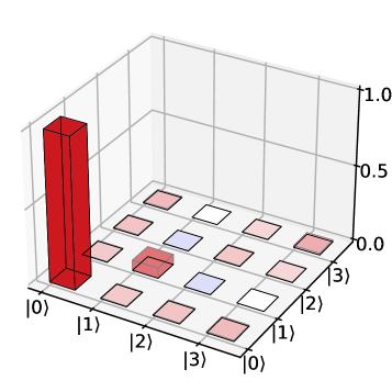
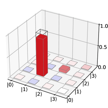
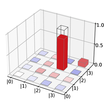
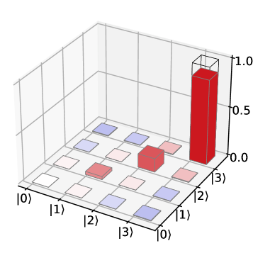
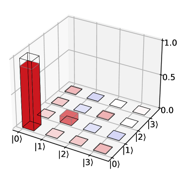
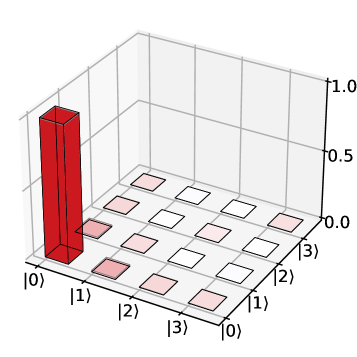
Figure 3: (a) to (d) show the real part of the measurement operators reconstructed from gate-set tomography (GST), which give the expectation value of transmon population in $\ket{0}$, $\ket{1}$, $\ket{2}$, and $\ket{3}$ states, respectively. The infidelity of these operators are $0.14\pm 0.24\times 10^{-2}$, $10.98\pm 0.25\times 10^{-2}$, $21.55\pm 0.03\times 10^{-2}$, $12.85\pm 0.23\times 10^{-2}$, respectively. Figures (e) and (f) show the real part of the density operator of the initial state without and with the active reset protocol enabled, respectively. The infidelity of the initial states are $9.9\pm 1.1\times 10^{-2}$ and $0.68\pm 0.13\times 10^{-2}$, without and with the active reset enabled, respectively.

After characterizing the initial state density operator, we observed a non-negligible population in the excited state, which prompted us to implement a qudit active reset protocol to prepare a high-fidelity initial state. We achieved this by utilizing the programmed FPGA to distinguish all four states using the nearest neighbor method with a duration of 40 ns, and sending a conditional sequence of $\pi$ pulses in the $\{\ket{2},\ket{3}\}$, $\{\ket{1},\ket{2}\}$ and $\{\ket{0},\ket{1}\}$ subspaces to reset the state back to the ground state. The effectiveness of the active reset protocol was verified by characterizing the initial state operator using GST. We found that the active reset significantly improved the initial state fidelity from $0.900\pm 0.011$ to $0.9932\pm 0.0013$, with twice repeated active reset being optimal. Prior to each following experiment, we applied the active reset protocol twice to ensure the preparation of a high-fidelity initial state.

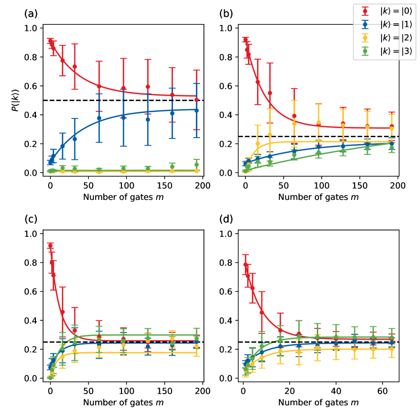
Figure 4: (a) and (b) show the results of single-qubit randomized benchmarking on the virtual qubits A and B of the emulator, yielding average infidelity per single qubit Clifford gate $1.91\pm 0.23\times 10^{-2}$ and $2.89\pm 0.31\times 10^{-2}$, respectively. (c) depicts the simultaneous randomized benchmarking of single-qubit gates on both virtual qubits, with gate sequences executed in series. The average infidelity per single-qubit Clifford is extracted to be $3.14\pm 0.26\times 10^{-2}$ (d) shows the results of full 2Q randomized benchmarking on the emulator, and the average infidelity per two-qubit Clifford gate is $9.51\pm 0.71\times 10^{-2}$.

To evaluate the performance of the emulator, we conducted RB on the virtual qubits A and B. This allowed us to investigate the cost overhead of the emulation and determine its effectiveness. We generated single-qubit randomized Clifford gate sequences and converted them to the native qudit gate using the simulator’s mapping rule. The RB sequences were run on the emulator, and the success probability $P$ was defined as the population landing on the emulated state $\ket{00}$. We fit the RB model to $P=Ap^{m}+B$, where $A$, $B$, and $p$ are fitting parameters, and $m$ is the number of Clifford gates. We calculated the average infidelity per Clifford as $r=(1-p)(d-1)/d$, where $d=2$ for single-qubit RB and $d=4$ for two-qubit RB. The resulting average single-qubit Clifford gate infidelity for virtual qubits A and B were $1.91\pm 0.23\times 10^{-2}$ and $2.89\pm 0.31\times 10^{-2}$, respectively. Notably, performing single-qubit RB on virtual qubit A only drives the population within the ${\ket{0},\ket{1}}$ subspace. Although transitions within the $\{\ket{2},\ket{3}\}$ subspace are driven, a negligible population exists in this subspace. Therefore, we expect $P$ to converge to $0.5$, unlike the rest of the RB experiments that converges to $0.25$. We also performed RB on both virtual qubits using the emulated single-qubit gates, yielding an average infidelity per Clifford of $3.14\pm 0.26\times 10^{-2}$. Finally, we implemented full two-qubit Clifford randomized benchmarking, with the two-qubit gate decomposition first decomposing the Clifford gate into a sequence optimized for the cross-resonance $ZX$ interaction. Then, these decomposed gates were mapped to the qudit intrinsic gate set. We extracted the average emulated two-qubit Clifford gate infidelity to be $9.51\pm 0.71\times 10^{-2}$. Our results suggest that emulating two qubits on qudit results in fidelity loss, highlighting the need for optimal mappings of the operations on the emulated qubits to the qudit to further improve performance.

VQE

Figure 5: Gate sequence for implementing the variational ansatz used to approximate the binding energy of a hydrogen molecule. The gates are mapped to the qudit native operations under the rules described in Fig. 1, and the $ZZ(\theta)$ gate is implemented by applying two virtual Z gates $Z_{1}(-\theta)$ and $Z_{2}(-\theta)$.

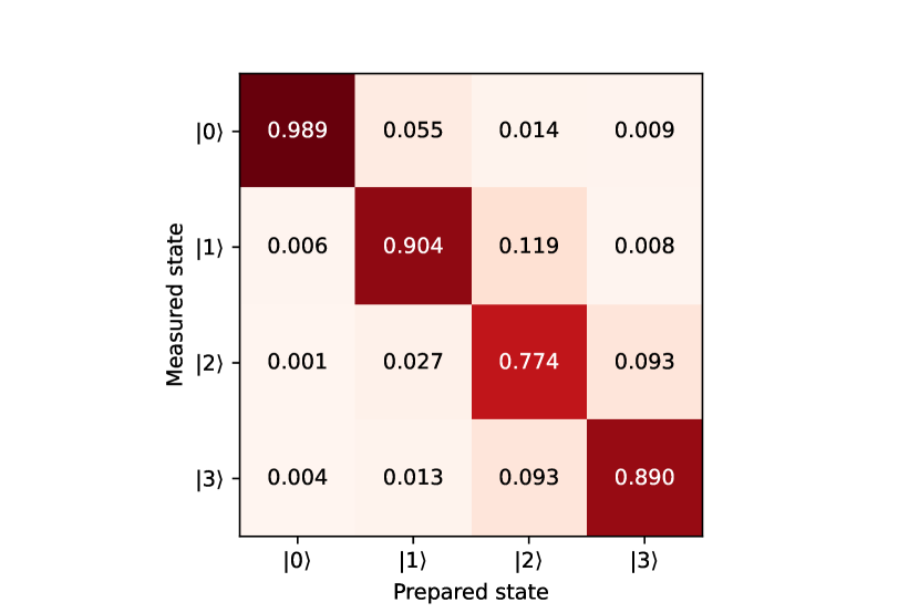
Figure 6: The assignment matrix measured during the execution of VQE sequences. The assignment matrix was used to implement measurement mitigation.

	Raw value	Outlier removed	Measurement mitigation	Simulation
IZ
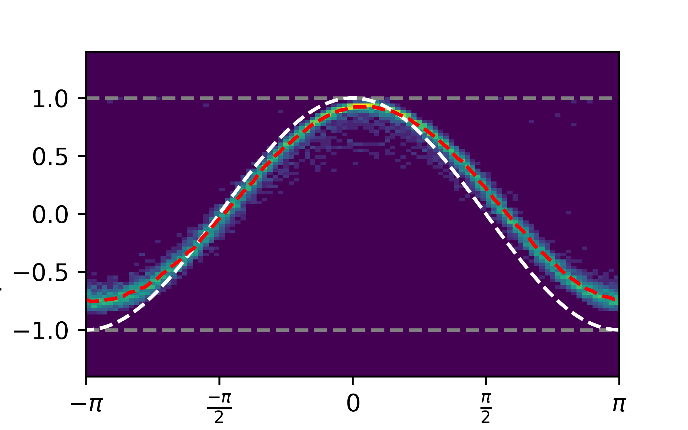
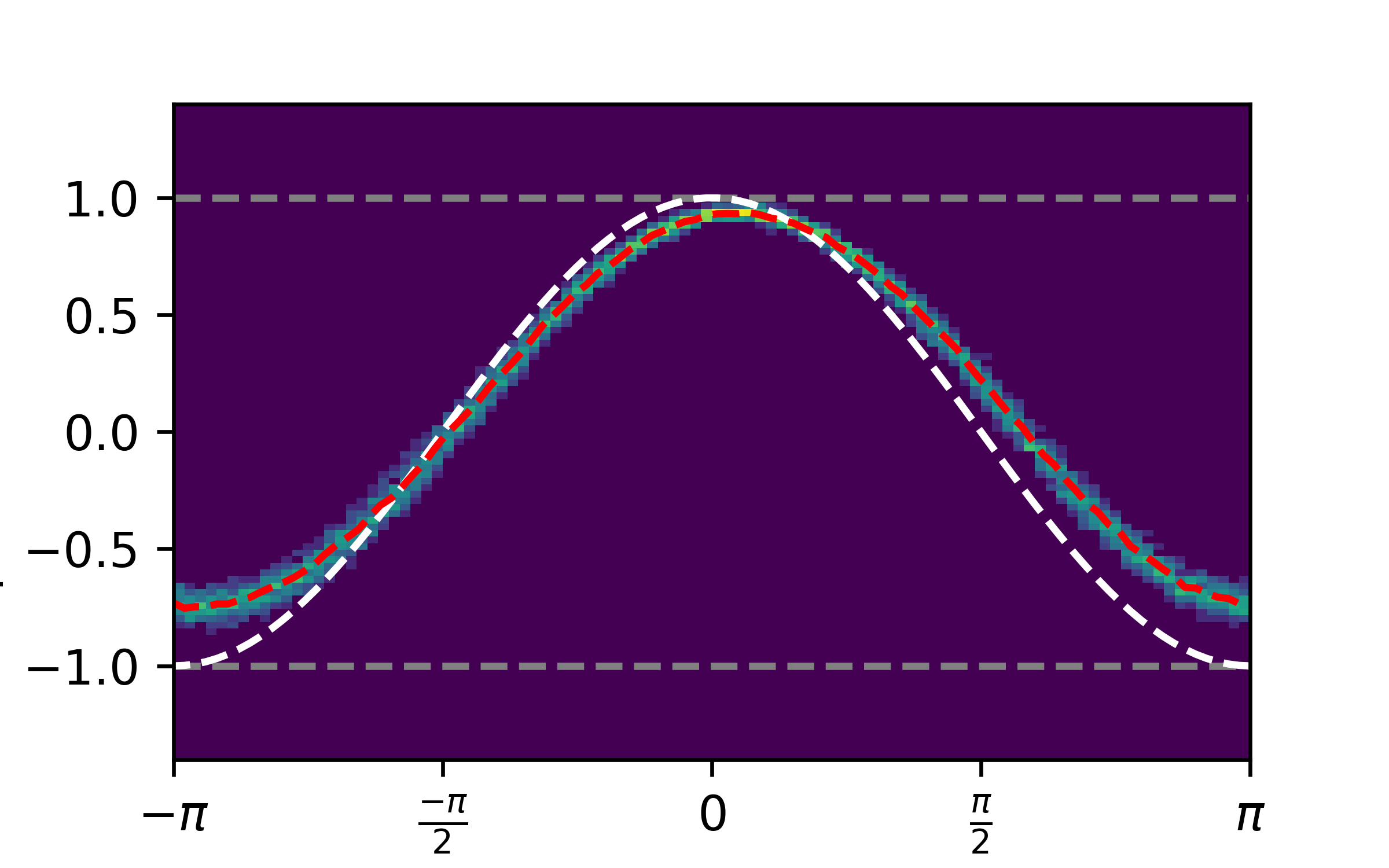
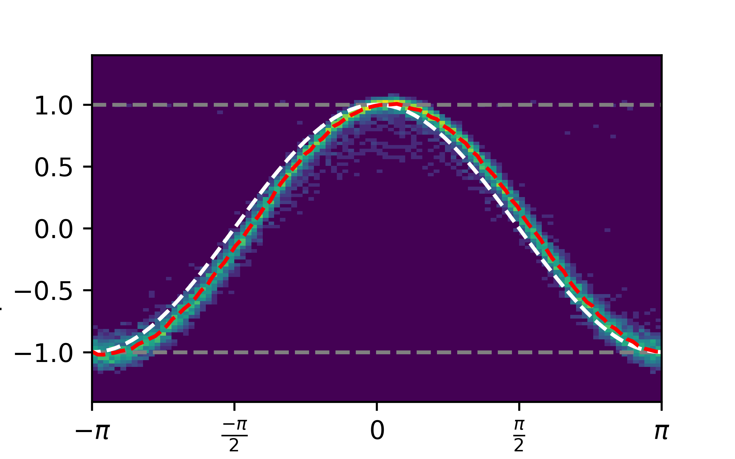
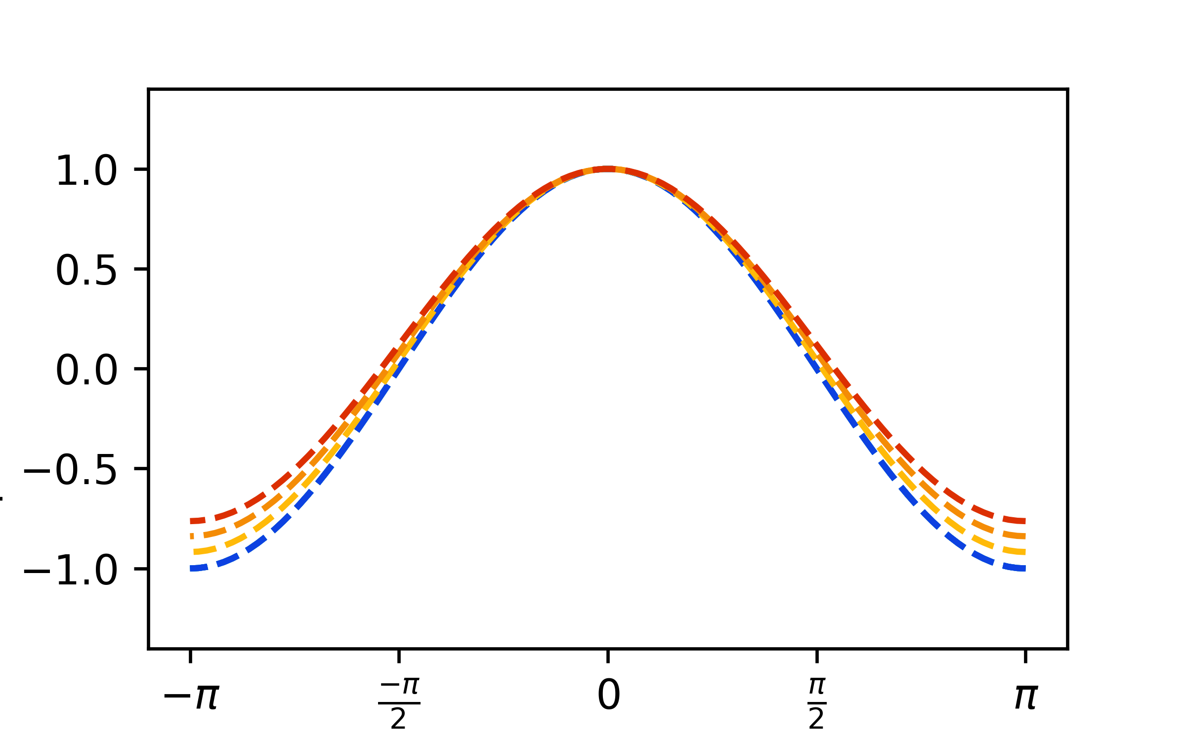
ZI
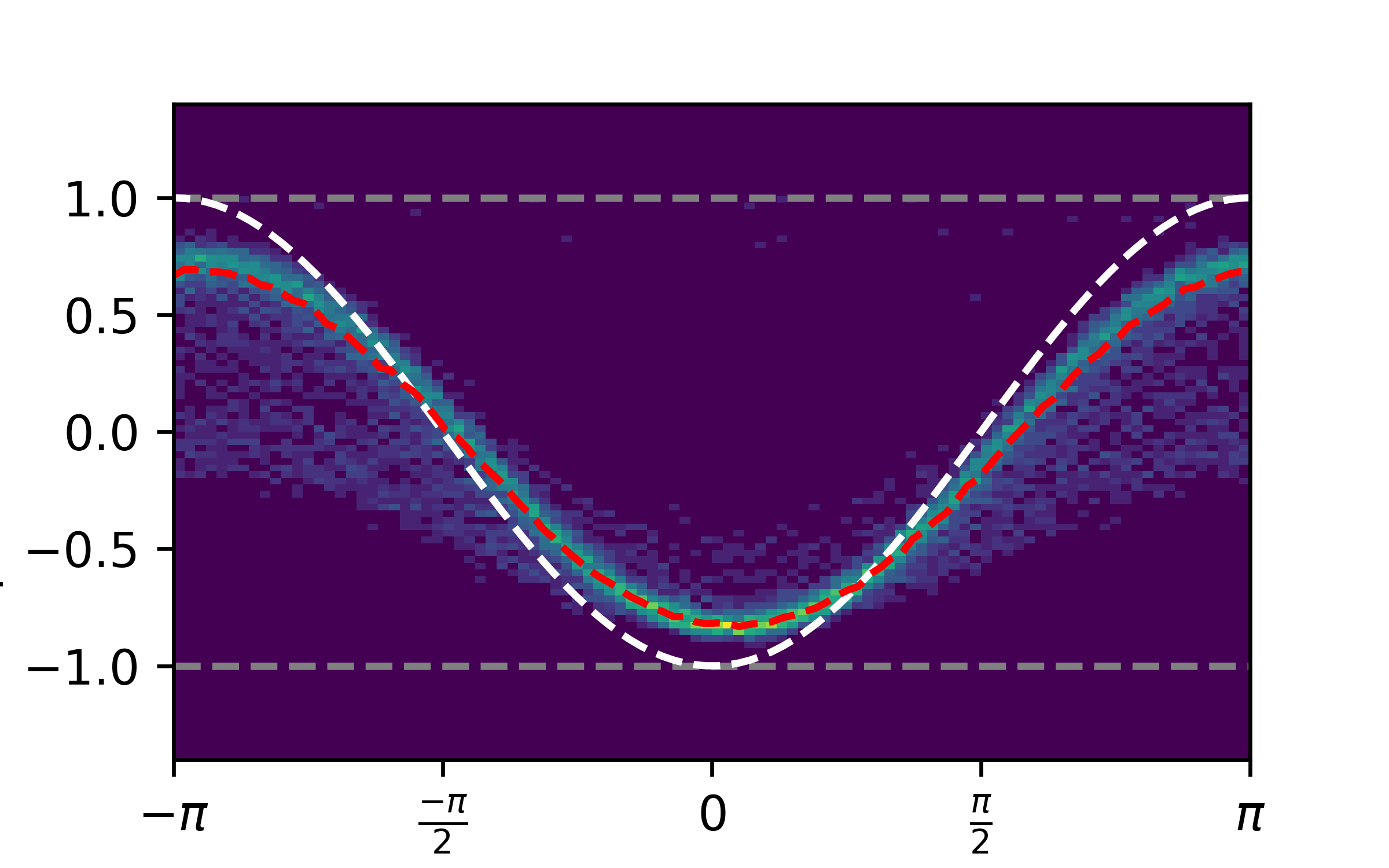
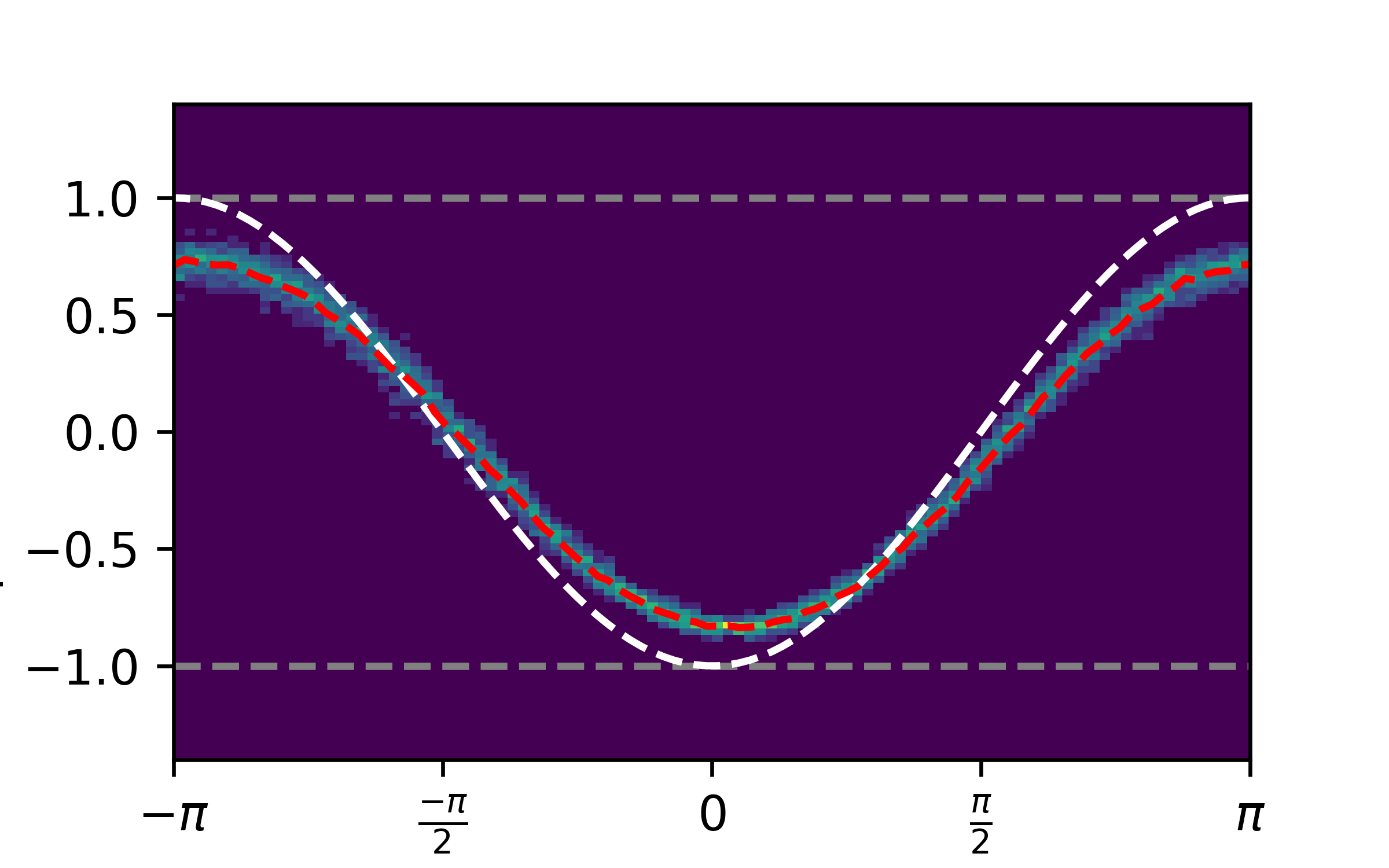
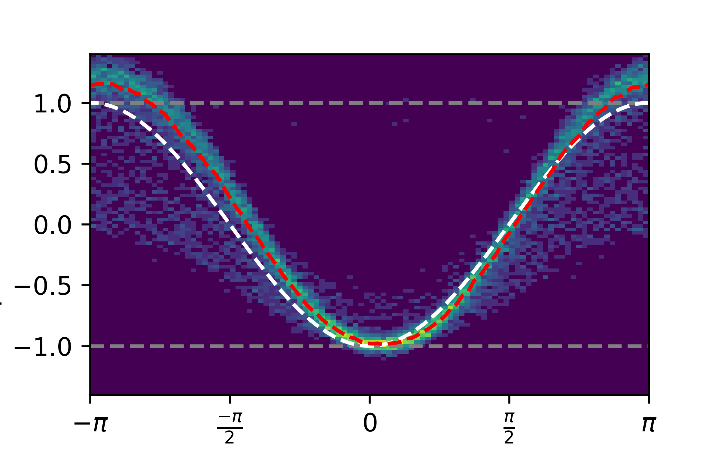
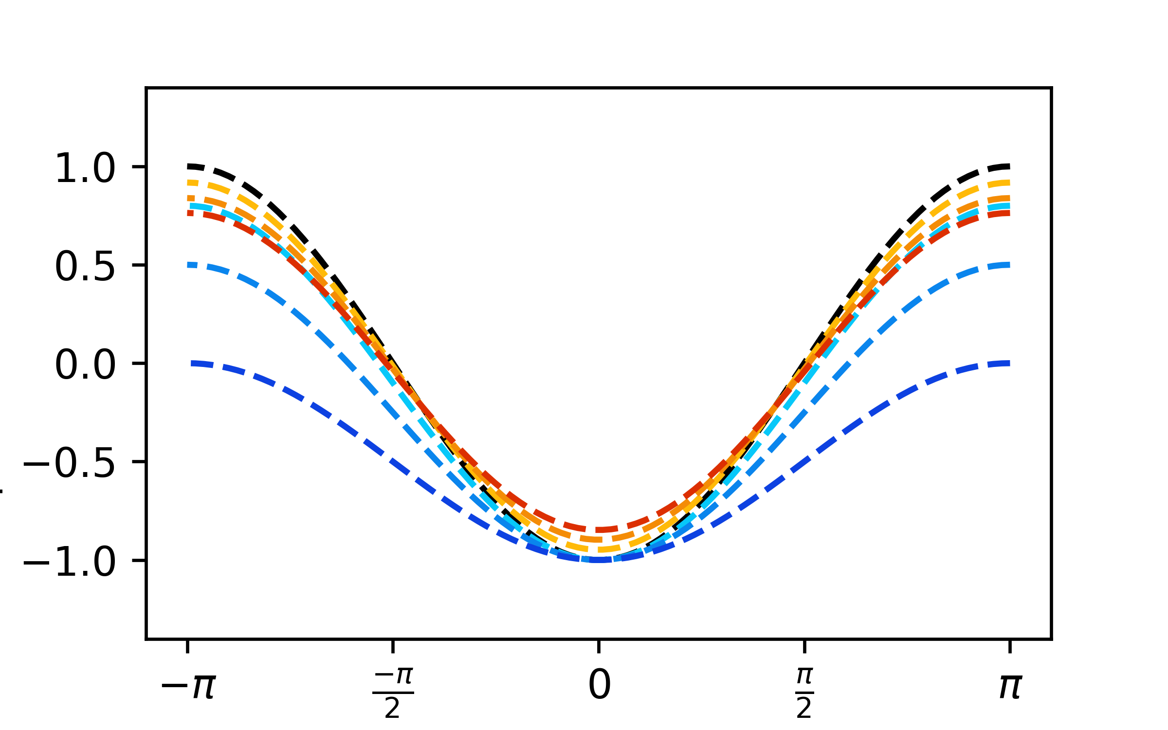
ZZ
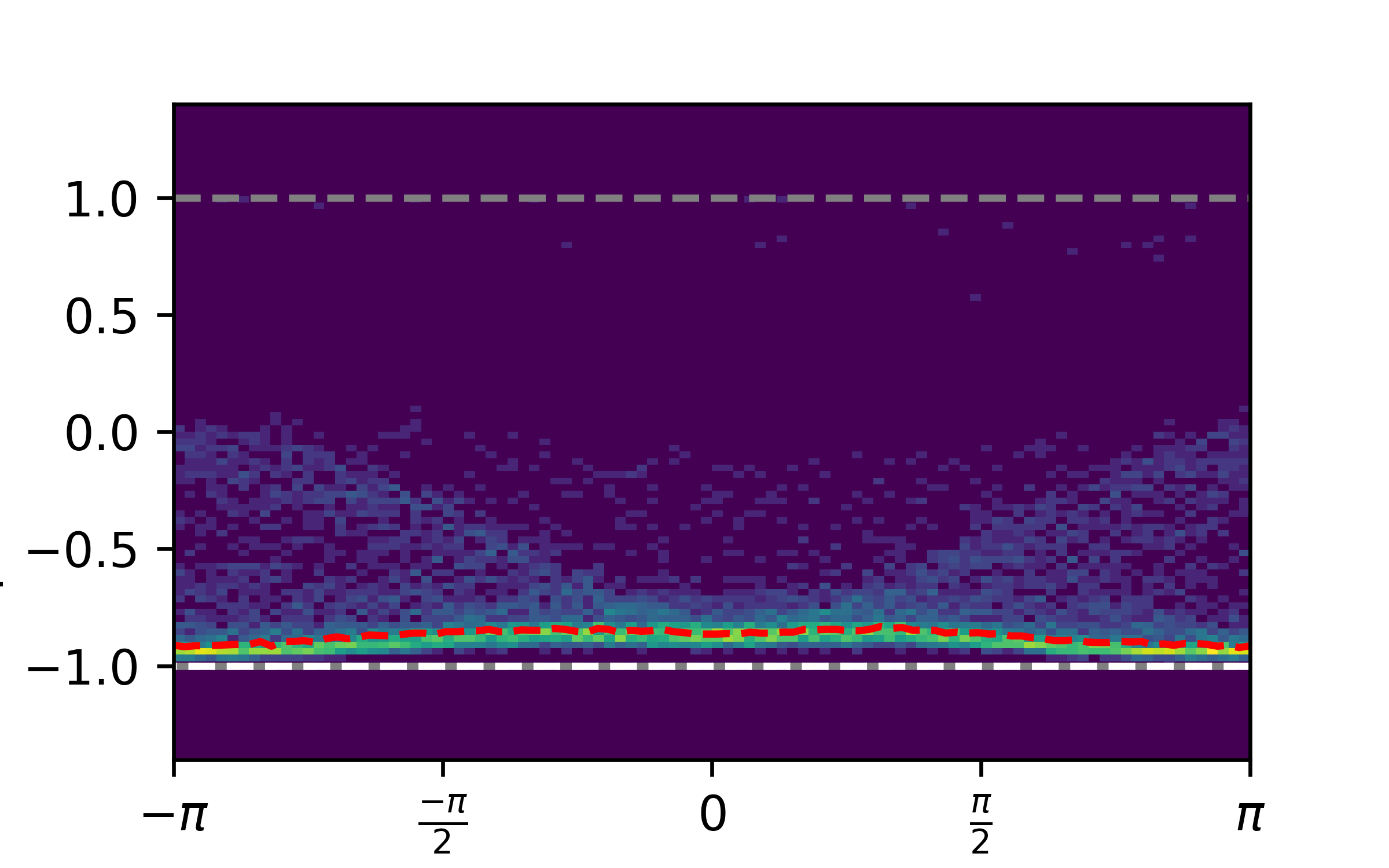
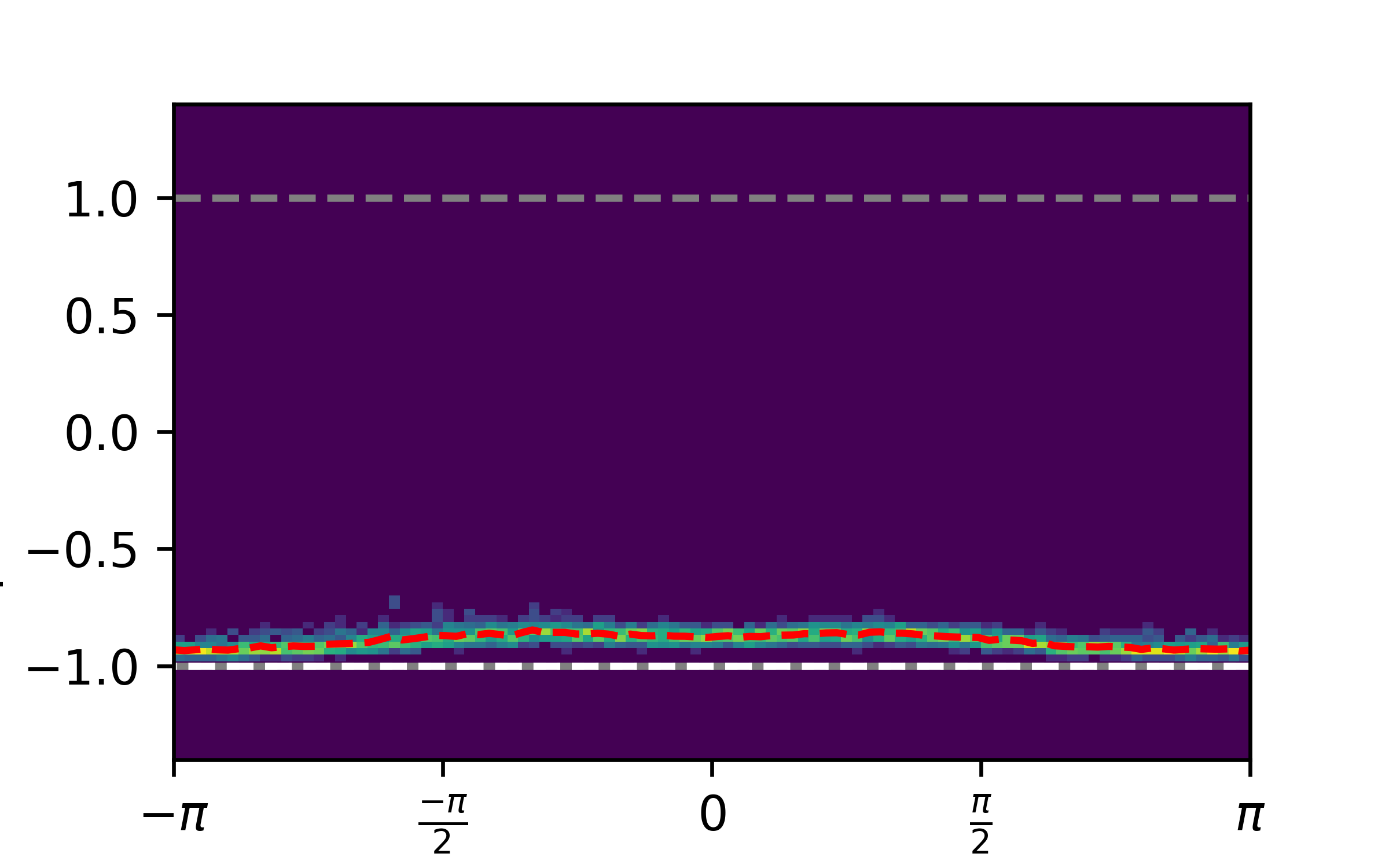
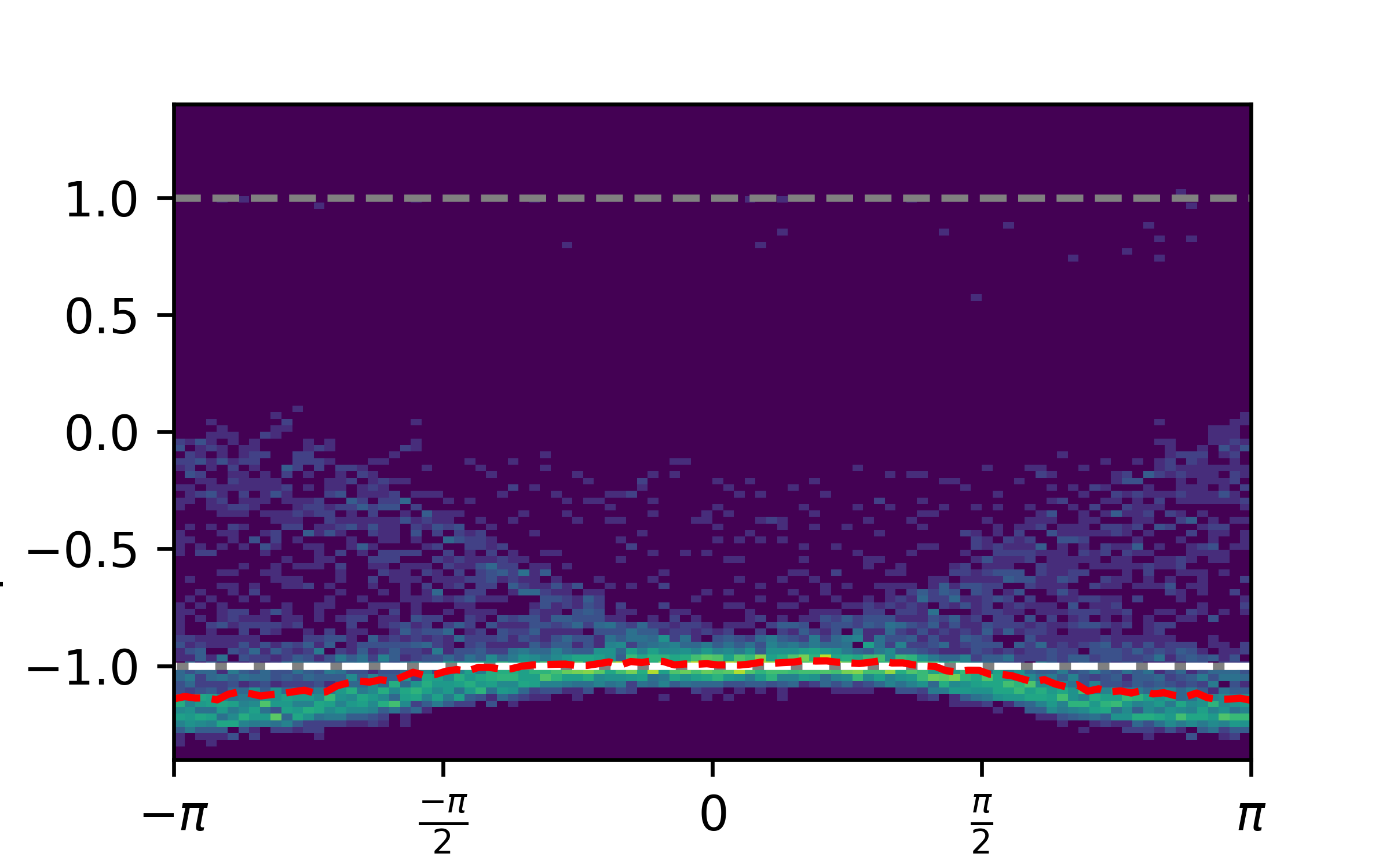
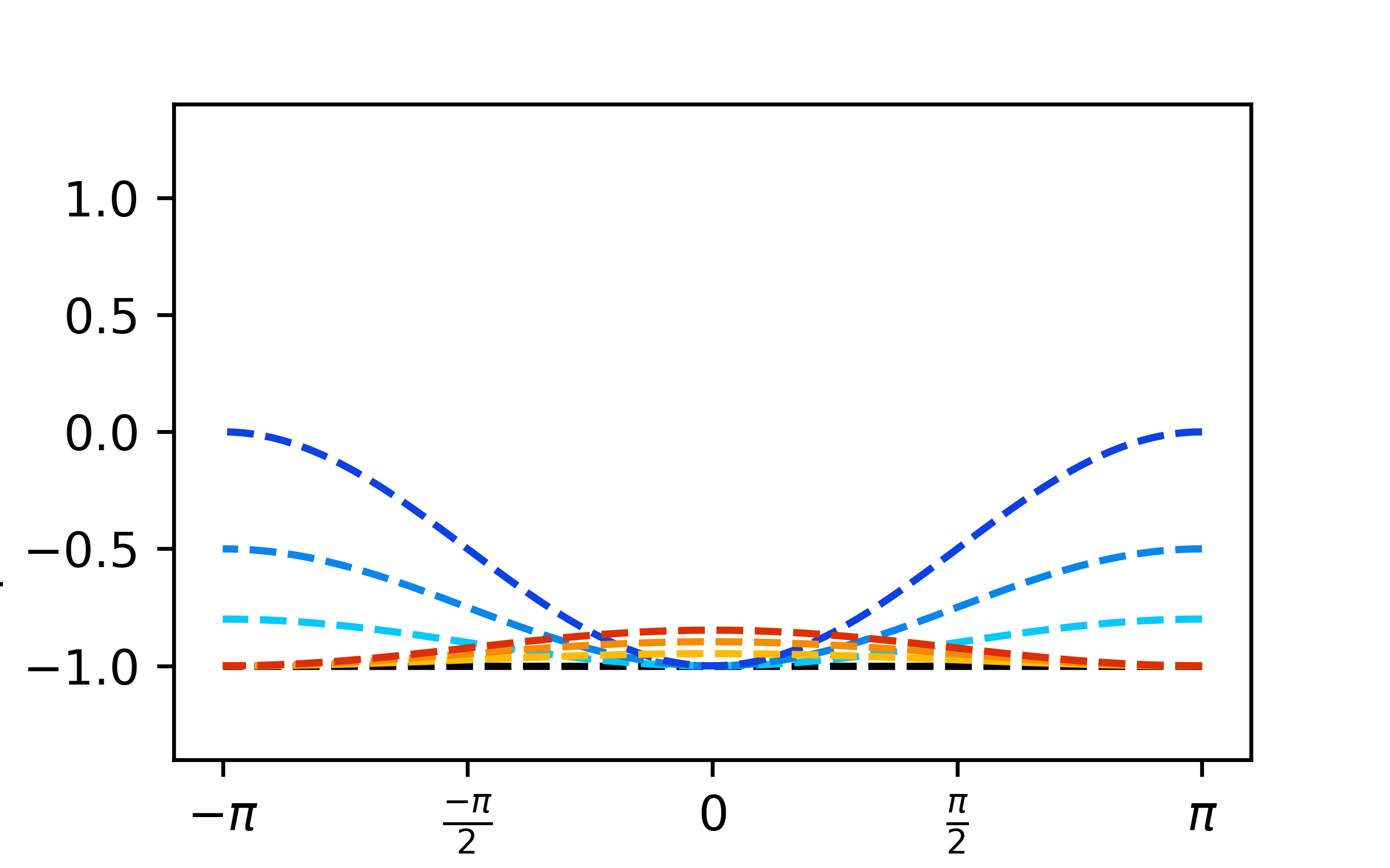
XX
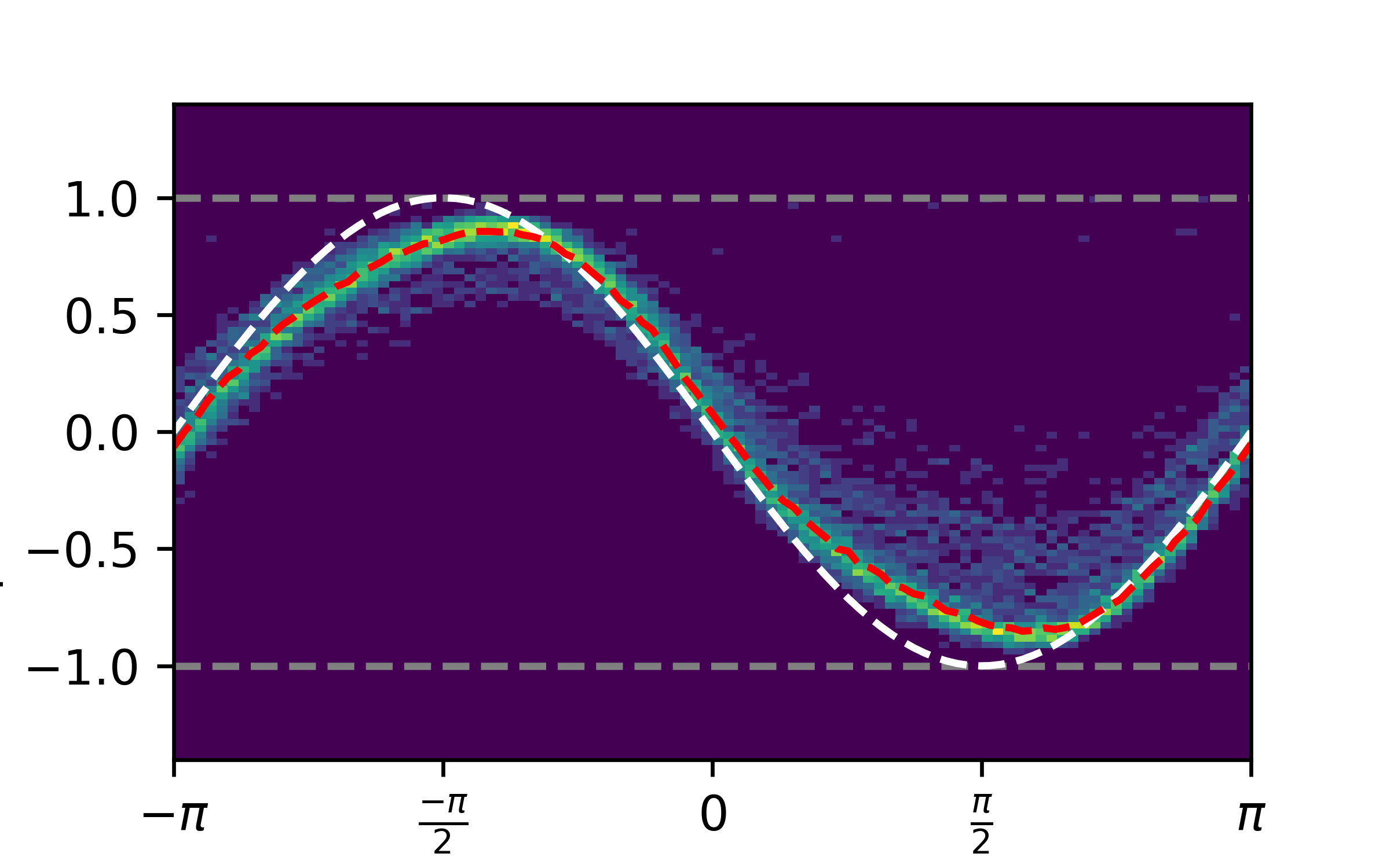
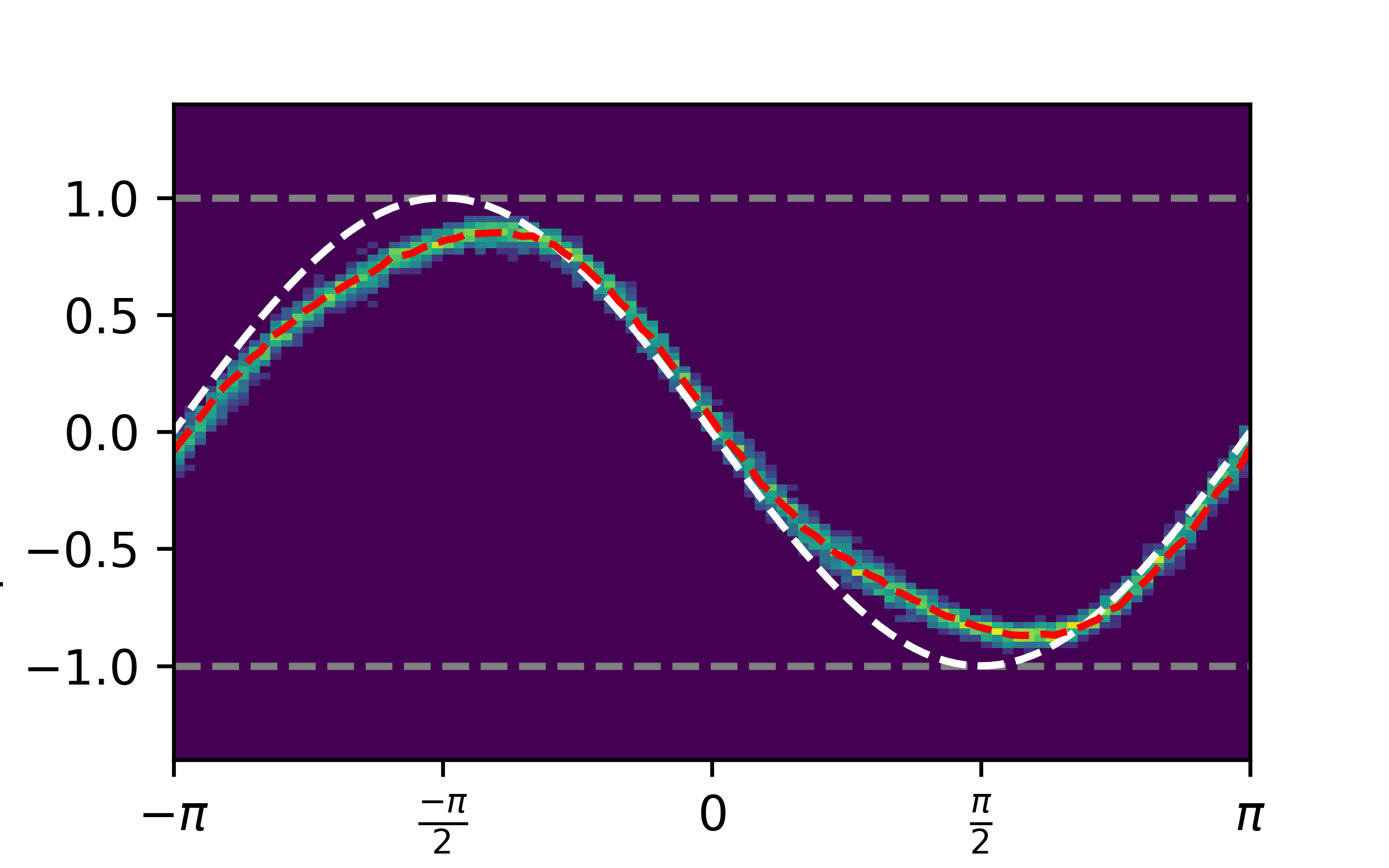
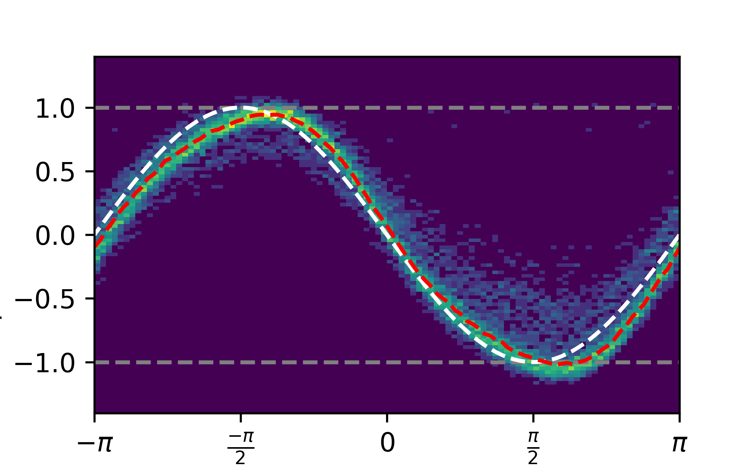
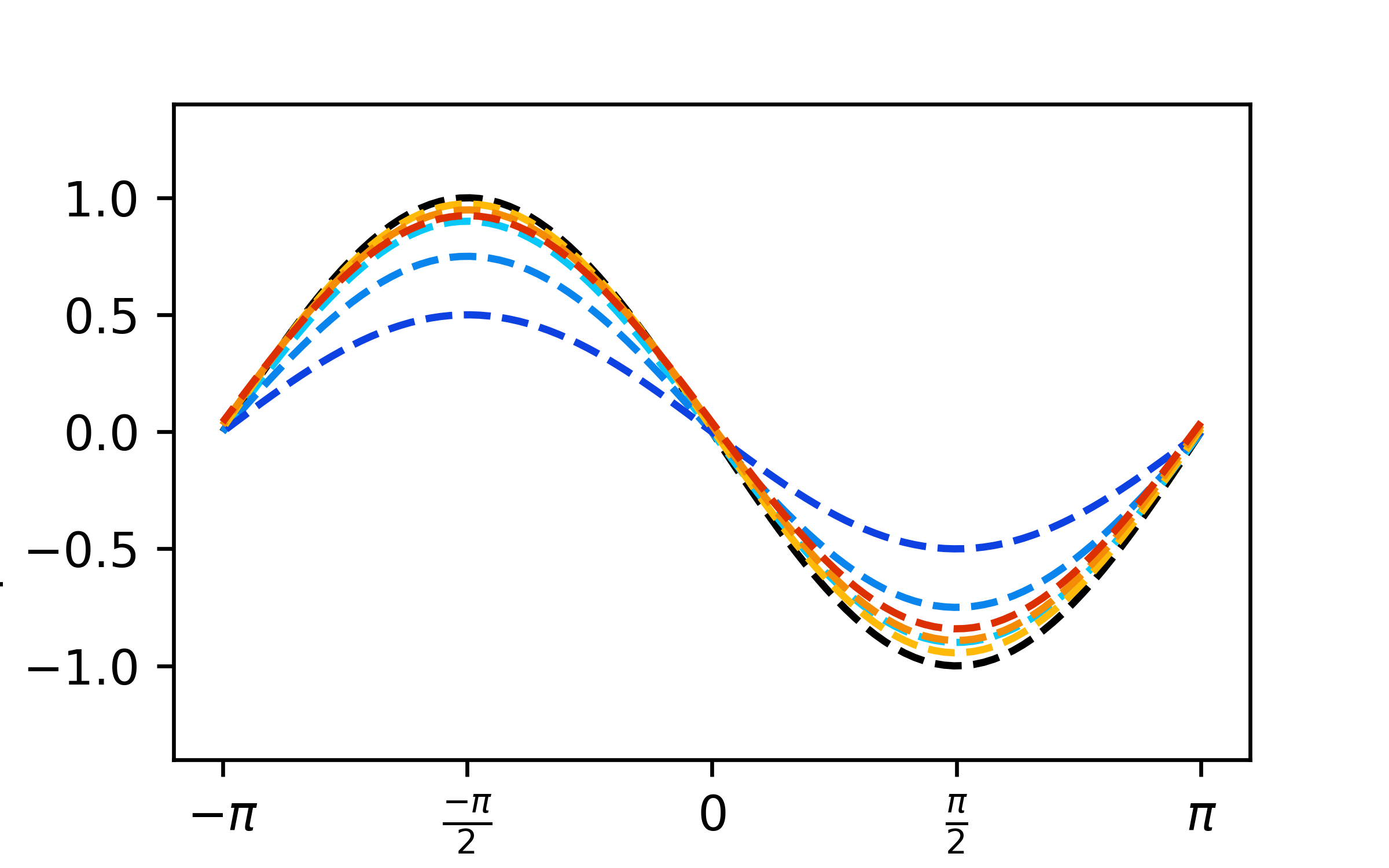
YY

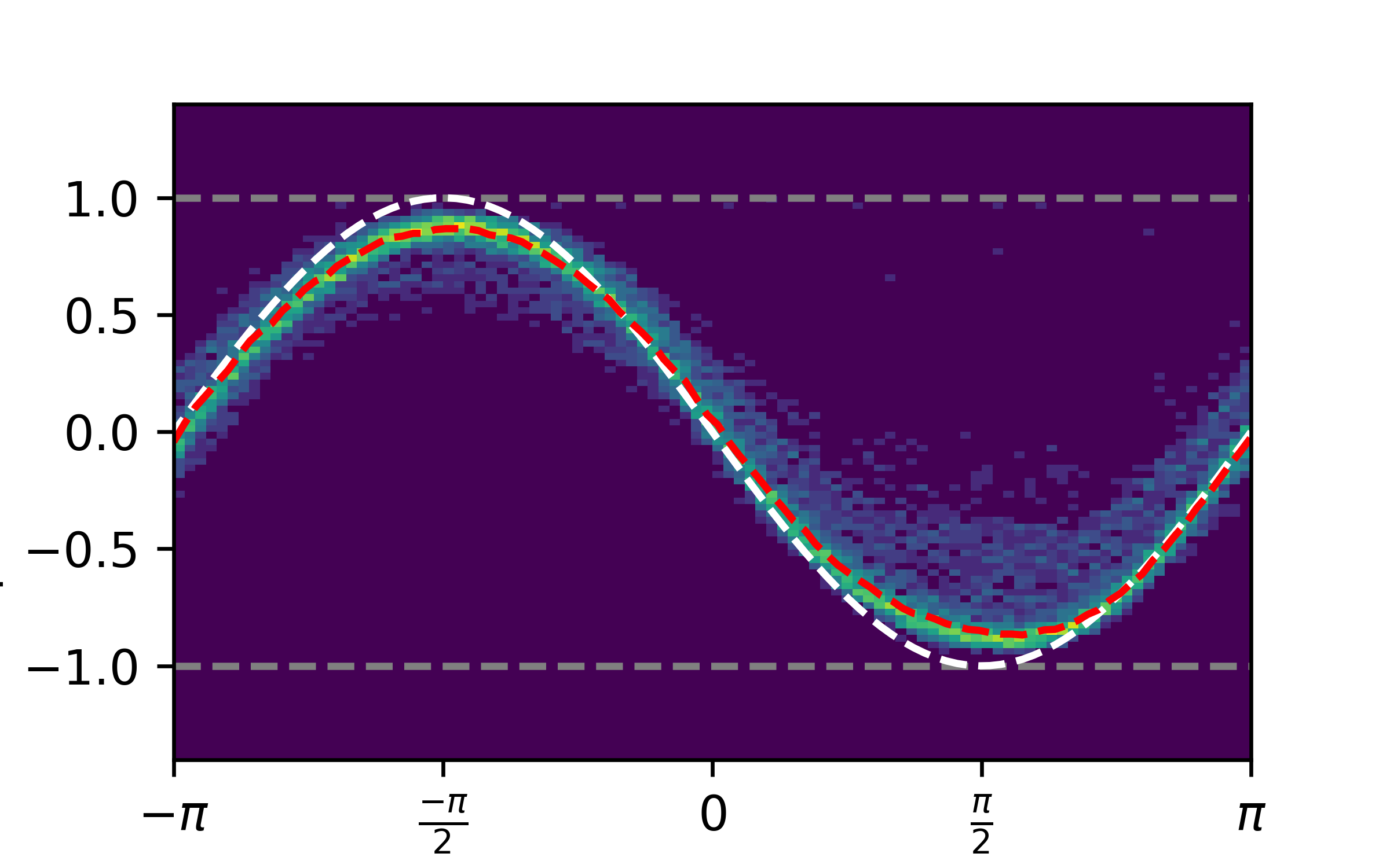
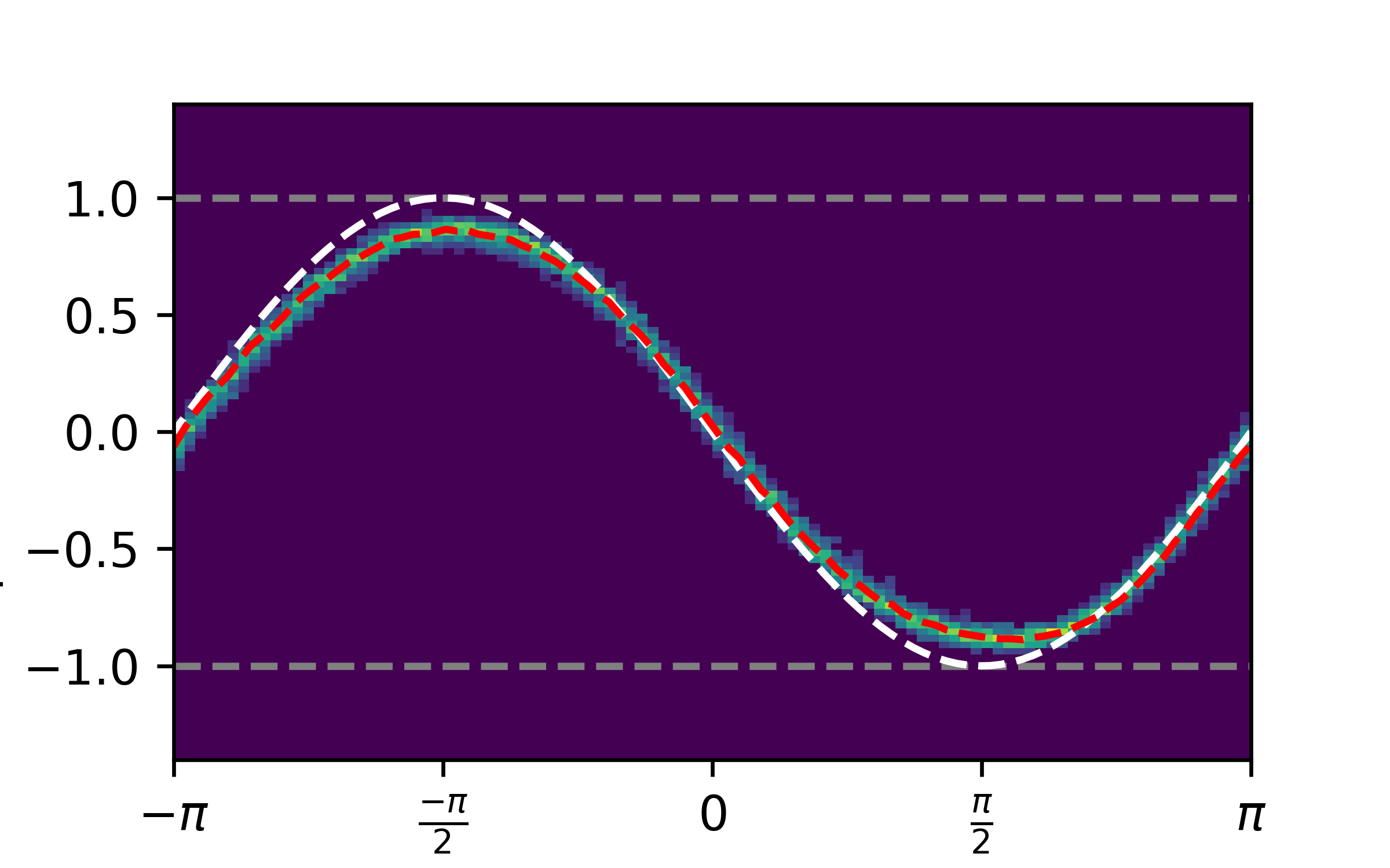
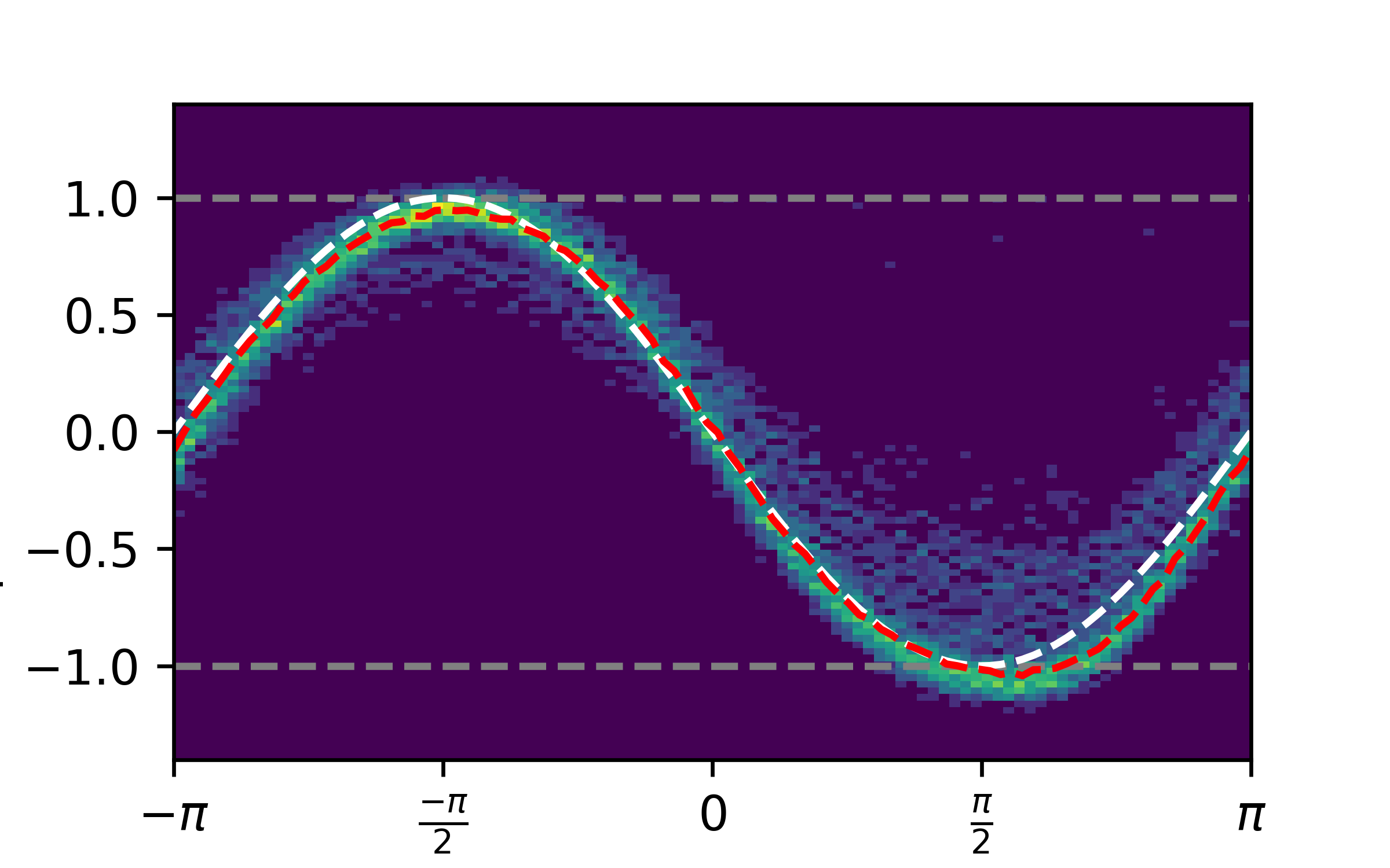
Figure 7: Experimental results are shown for the expectation values of each Pauli operator as a function of the ansatz parameter in the VQE used to determine the binding energy of a hydrogen molecule. The VQE ansatz is implemented using the gate sequence shown in Fig. 5. The white dashed curve represents the theoretically expected ground truth obtained by simulating the ansatz classically. The red curve represents the averaged expectation value of the distribution. The first column shows the raw experimental data. In the second column, the experimental data has been processed to remove $50\%$ of the population using Gaussian distribution outlier detection to eliminate misclassification events. The third column shows the expectation values after applying assignment mitigation. The last column displays the simulated expectation values versus the parameter under the amplitude damping noise (red) and misclassification noise (blue). The colors from light to dark denote the strength of the error. The black line denotes the simulated expectation value without noise.

The Variational quantum eigensolver (VQE) is a promising application of near-term quantum devices Cerezo et al. (2021); Tilly et al. (2021), which has been used to solve electronic structure problems such as the bonding energy of a hydrogen molecule. This particular problem requires a minimum of two qubits using the symmetry-conserving Bravyi-Kitaev encoding of the Hamiltonian O’Malley et al. (2016); Kandala et al. (2017); Bravyi et al. (2017). As an evaluation of the practicability of the emulator, we use a 4-level qudit system to emulate this two-qubit system and demonstrate VQE on a qudit.

To solve electronic structure problems, the VQE optimizes a wave function with a pre-assumed form, or ”ansatz” $\ket{\Psi}$. The variational principle guarantees that the ground-state energy of the electronic system, denoted as $E_{0}$, can be approximated by optimizing the parameters $\vec{\theta}$ in the ansatz $\ket{\Psi(\vec{\theta})}$. It can be written as $\bra{\Psi(\vec{\theta})}H\ket{\Psi(\vec{\theta})}\geq E_{0}$, where $\ket{\Psi(\vec{\theta})}$ is the ansatz parametrized by $\vec{\theta}$, and $H$ is the Hamiltonian. The wave function is typically generated using a parametrized quantum circuit, and in this case, we use the ansatz $\ket{\Psi(\vec{\theta})}=e^{-i\theta XY}\ket{\Psi_{\mathrm{HF}}}$, which is suggested from the unitary coupled cluster theoryO’Malley et al. (2016); Anand et al. (2022); Romero et al. (2018). $\ket{\Psi_{\mathrm{HF}}=\ket{01}}$ is the Hartree-Fock state which is used as a starting point in the unitary coupled cluster theory, and where it is assumed electrons occupy the lowest lying orbitals.

We implement the chosen ansatz on the two-qubit emulator using the gate sequence shown in Fig. 5. The energy of the hydrogen molecule is evaluated as $E(\vec{\theta})=\bra{\Psi(\vec{\theta})}H\ket{\Psi(\vec{\theta})}=\sum_{i}g_{i}\bra{\Psi(\vec{\theta})}P_{i}\ket{\Psi(\vec{\theta})}$, where $P_{i}\in\{IZ,ZI,ZZ,XX,YY\}$ and $g_{i}$ are coefficients that can be computed from the hydrogen bond distance $R$. The measurement of the quantum state gives the probability distribution of the state in $\ket{0}$, $\ket{1}$, $\ket{2}$, and $\ket{3}$, which we represent as a vector $R=\{p_{\ket{0}},p_{\ket{1}},p_{\ket{2}},p_{\ket{3}}\}$. The expectation value for an operator $M\in{IZ,ZI,ZZ}$ is evaluated as $\braket{M}=\mathrm{diag}(M)^{T}R$. The $\braket{XX}$ and $\braket{YY}$ are measured by swapping the $X$ or the $Y$ basis with $Z$ basis of both qubits , respectively, and measure $\braket{ZZ}$. There is only one parameter in the ansatz; in the experiment, the parameter is swept 100 points from $-\pi$ to $\pi$. Each point is sampled 10,000 times, each time uses 500 shots to estimate the expectation value. The distribution of the estimated expectation value is displayed in the form of a heatmap in Fig.7. The solved energy versus the hydrogen bond distance is given in Fig.8.

In comparison to the simulation results, the experimental data displays some noticeable differences. As shown in Figure 7, we observe that the amplitude of the expectation value for all operators is lower than 1, whereas in the simulation, it should be 1. Additionally, the $ZZ$ expectation value exhibits a larger value when the parameters are set to 0 compared to $\pi$, which is not the case in the simulation where it remains constant. Moreover, the distribution plot for each expectation value shows a ”shadow,” indicating that some of the measured distributions are not well-approximated by a simple Gaussian distribution. These results suggest that the system is subject to a complex noise model. We consider two potential sources of error for this result: (1) amplitude damping error during the long measurement time, and (2) misassignment between the $\ket{2}$ and $\ket{3}$ states, as indicated by GST. We use simulations to investigate the impact of these two types of noise and compare the simulated expectation value with the experiment result.

To address the misclassification event between the $\ket{2}$ and $\ket{3}$ states, we introduced a readout model $\tilde{P}(\ket{2})=(1-\epsilon)P(\ket{2})+\epsilon P(\ket{3})$ and $\tilde{P}(\ket{3})=(1-\epsilon)P(\ket{3})+\epsilon P(\ket{2})$, where $\tilde{P}(\ket{i})$ is the measured probability for state $\ket{i}$ under the noise model. The blue line in the simulation figures represents the simulated expectation value versus parameter under the misclassification noise, with $\epsilon$ values of $0.1$, $0.25$, and $0.5$, where lighter colors indicate lower noise strength and darker colors indicate higher noise strength.The simulation result reveal that this misclassification event is likely the cause of the observed ”shadow” in the distribution of the expectation values.

For the amplitude damping channel, we introduce a completely positive trace preserving (CPTP) channel operator $\mathcal{D}$ for a qudit to describe the amplitude damping error Nielsen and Chuang (2000); Chessa and Giovannetti (2021). Here we use $\mathcal{D}(\rho)=K_{0}\rho K_{0}^{\dagger}+\sum_{0\leq i<j<d-1}K_{ij}\rho K_{ij}^{\dagger}$, where $K_{ij}=\sqrt{\gamma_{ij}}\ket{i}\bra{j},\forall i,j~{}\mathrm{s.t.}~{}0\leq i<j<d-1$ and $K_{0}=\ket{0}\bra{0}+\sum_{1\leq j<d-1}\sqrt{1-\xi_{j}}\ket{j}\bra{j}$. $\gamma_{ji}$ has real value, describs the decay rate from the $j$-th to the $i$-th level ($\xi_{j}=\sum_{0\leq i<j<d-1}\gamma_{ji}\leq 1$). We performed simulations using the error model described above and set $\gamma_{ji}=1-\exp(-t\Gamma_{ji})$, where $1/\Gamma_{ji}$ is the effective $T_{1}$ for the $\{\ket{i},\ket{j}\}$ subspace and $t$ is the simulated waiting time for the decay of the system. We used $t=5,10,15\mathrm{~{}\mu s}$ for the red curves from light to dark, respectively. The simulation results indicate that the distortion of the $ZZ$ expectation value is similar to the simulated value from the amplitude-damping channel. This suggests that the amplitude damping error during the measurement is likely to be the main source of error for the $ZZ$ expectation value.

To mitigate the effect of the misclassification error, a Gaussian fit is applied to the measured probability distribution to identify and remove the outliers that contribute to the ”shadow” in the distribution . We exclude $50\%$ of the population as outliers to visually eliminate all the “shadow”, and show the remaining population in the ”Outlier removed” column of Fig. 7. The resulting expectation values, shown in blue in Fig. 8, have significantly reduced error bars compared to the raw results. However, there is still a noticeable difference between the VQE result and the Hamiltonian diagonalization result.

To mitigate both the readout assignment error and the amplitude damping error during measurement, we applied measurement assignment mitigation using the assignment matrix $A$. This matrix describes the probability of measuring the state $\ket{j}$ when the system is prepared in state $\ket{i}$, and was used to obtain a mitigated probability distribution $\tilde{R}$ by inverting the assignment matrix as $\tilde{R}=A^{-1}R$. The mitigated expectation value was then evaluated as $\braket{\tilde{M}}=diag(M)^{T}A^{-1}R$. The measured assignment matrix is shown in Fig. 6. Notable misclassification between the $\ket{2}$ and $\ket{3}$ states is observed, consistent with data from gate-set tomography. The result after mitigation is shown in green in Fig. 8. By applying the measurement assignment mitigation technique, we were able to decrease the difference between the averaged solved energy and the Hamiltonian Diagonalization result to below the chemical accuracy threshold of $1.5\times 10^{-2}$ Hartree O’Malley et al. (2016). However, due to the large misclassification error, the error bar remains significant.

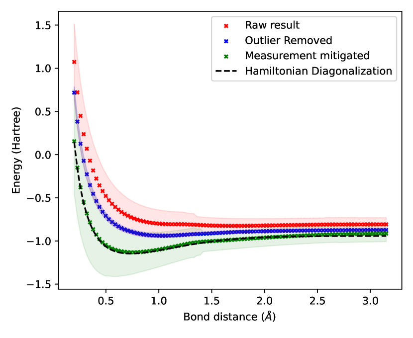
Figure 8: The energy of the hydrogen molecule as a function of bond distance, obtained by the variational quantum eigensolver (VQE). The crosses represent the average energy value from multiple experiments, while the colored shadow indicates the error bar corresponding to one standard deviation. The error bar is evaluated by propagating the uncertainty of each Pauli operator expectation value to the evaluated energy. The black line represents the energy of hydrogen obtained by diagonalizing the Hamiltonian.

Discussion

This work aims to explore the potential of high levels in a transmon as a computational space for near-term quantum applications. By introducing higher levels, we increase the Hilbert space available for quantum algorithms, which can lead to more efficient and powerful algorithms. However, there are two main challenges to overcome: higher levels can introduce additional noise, and recompilation of the algorithm is necessary to fully utilize the extended Hilbert space. In this work, we demonstrate a high-coherence transmon device as a 2-qubit emulator to address these challenges.

We conduct detailed characterizations and benchmarking on both the hardware and the emulator, including active reset to prepare a high-fidelity initial state. We then implement variational quantum algorithms on the qudit device, confirming that charge noise at higher levels is not detrimental for the algorithm. The main source of error is the decay that occurs during the measurement process. We then mitigate this error with post-processing techniques and obtain a solution for the energy of a Hydrogen molecule with an error within chemical accuracy.

One direction for future work is to study the entanglement properties of multilevel transmons. Additionally, further exploration of the impact of higher levels on the noise and error rates of the device could help improve its overall performance. Overall, this work provides a significant step forward in the utilization of multilevel transmon systems for near-term quantum applications, and opens up exciting possibilities for future research in this field.

Appendix A Dispersive readout for qudits

The Jaynes-Cummings Hamiltonian in the dispersive limit can be used to describe the Hamiltonian of a qubit-resonator system with capacitive coupling Bianchetti et al. (2009, 2010). The Hamiltonian takes the form:

$$\mathcal{H}=\hbar\omega_{r}a^{\dagger}a+\sum_{k=0}^{n}\hbar\omega_{k}\ket{k}\bra{k}+\sum_{k=1}^{n-1}\hbar\chi_{k-1}\ket{k}\bra{k}+\sum_{j=0}^{n-1}\hbar s_{j}\ket{j}\bra{j}a^{\dagger}a$$ (1)

where $g_{j}$ is the coupling strength to the transmon transition $j$ and $j+1$, and $\Delta_{j}$ is the detuning between the resonator frequency and the $j$ and $j+1$ transition frequency. The resonator exhibits a dispersive shift $s_{j}=-(\chi_{j}-\chi_{j-1})$ from interaction with the transmon in state $\ket{j}$. Here, we define $\chi$ as $\chi_{1}=-s_{1}$ to maintain consistency with the conventions in most of the transmon literature. The transmon frequency also experiences a ”Lamb shift” that depends on the photon number within the resonator.

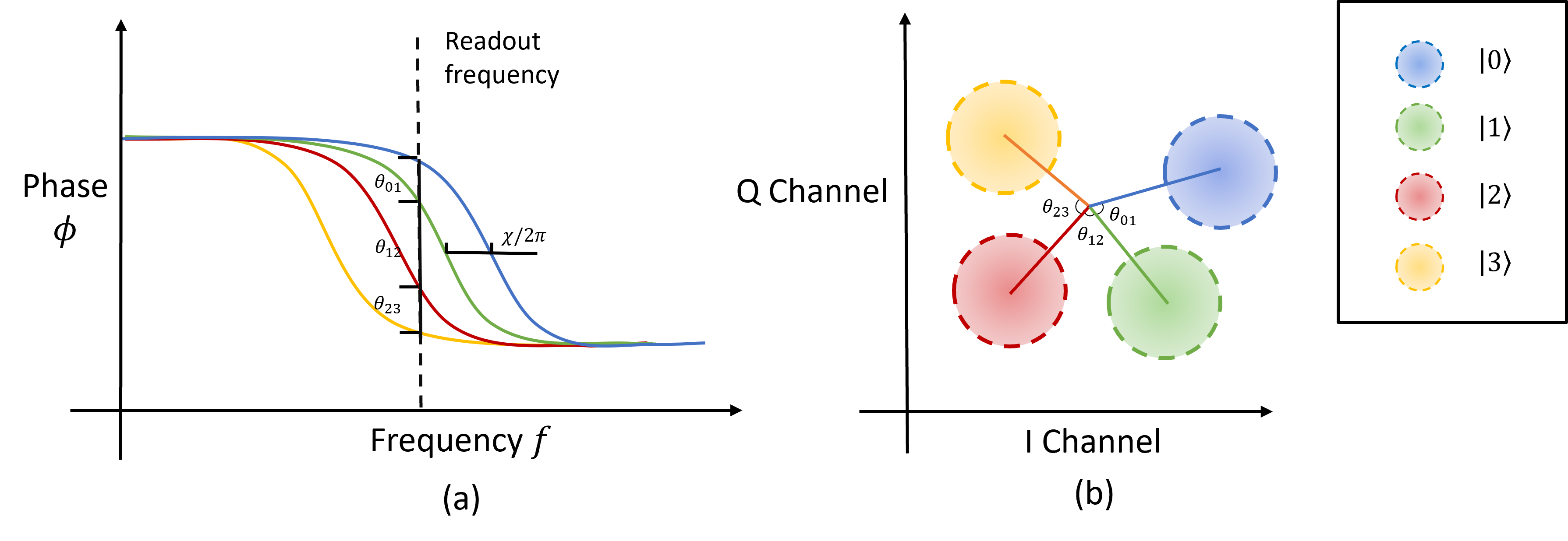
Figure 9: (a) plot shows the spectroscopy phase response of a resonator coupled to a qubit. The resonator oscillation frequency shifts depends on the transmon’s states, resulting in different phase responses shown in different colors. To read all four levels simultaneously, a readout signal is sent to the resonator with a frequency that maximally distinguishes the phase response of all four different states. (b) The scatter plot shows the I channel signal and Q channel signal, often referred to as the ”IQ plane.” The integrated sum of the demodulated signal over time gives a point on the IQ plane. The four different states correspond to four different regions on the IQ plane, whose size is determined by the measurement noise. The separation angle $\theta_{ij}$ between region $i$ and $j$ is related to the frequency shift shown in (a).

The above analysis demonstrates that the resonance frequency of the coupled resonator is dependent on the state of the transmon qubit, allowing the transmon state to be inferred by probing the resonator’s frequency. Since the dispersive shift is typically small, it is easier to distinguish the transmon state by the phase of the probing signal. A typical reflection response from a resonator is shown in Figure 9. The resonator phase response is shifted in the left figure, and by choosing a center frequency that can distinguish more signals, a single pulse can distinguish multiple states. Typically, the device is designed to have $\chi=\kappa$ so that a readout frequency can be chosen to make $\theta_{01}=\pi$, maximizing the readout fidelity. However, for reading out four different states simultaneously, we would like to have $\theta_{01}\approx\theta_{12}\approx\theta_{23}\approx\pi/2$, which can be approximately achieved by setting $\chi=\kappa/2$.

Appendix B Virtual Z gate

The physical drive implements the X or Y rotation in a qubit-like subspace. The Z rotation can be implemented virtually by shifting the phase of all gates in the rest of the sequence McKay et al. (2017). The implementation of the Z rotation for a multi-level system is with an extension of qubit virtual $Z$ gate. Suppose we would like to implement a Z gate in the following gate sequence.

$$U=G_{n}G_{n-1}...G_{k}Z_{m}(\theta)G_{k-1}...G_{0}$$ (2)

where $G_{k}$ denotes a gate. Now insert an identity gate sequence $Z_{m}(\theta)Z_{m}^{-1}(\theta)$ between all the following gates, and we get

$$U=Z_{m}(\theta)Z_{m}^{-1}(\theta)G_{n}Z_{m}(\theta)Z_{m}^{-1}(\theta)...Z_{m}(\theta)Z_{m}^{-1}(\theta)G_{k}Z_{m}(\theta)G_{k-1}...G_{0}$$ (3)

which is equivalent to the original gate sequence. Now we rewrite the $G_{k}^{\prime}=Z_{m}^{-1}(\theta)G_{k}Z_{m}(\theta)$ and get a new sequence

$$U=Z_{m}(\theta)G_{n}^{\prime}G_{n-1}^{\prime}...G_{k}^{\prime}G_{k-1}...G_{0}$$ (4)

where $G_{k}^{\prime}$ is implemented by shifting the phase of driving pulses. The last gate $Z^{-1}_{m}(\theta)$ will not make any difference if the state is measured with an operator commutes with $Z_{m}^{-1}(\theta)$, which is always the case for the standard dispersive readout. For a four-level qudit system, the virtual Z gate can be implemented as shown in table 1 .

	$\{\ket{0},\ket{1}\}$ subspace	$\{\ket{1},\ket{2}\}$ subspace	$\{\ket{2},\ket{3}\}$ subspace
$Z^{1}(\theta)$	$-\theta$	$\theta$	0
$Z^{2}(\theta)$	$0$	$-\theta$	$\theta$
$Z^{3}(\theta)$	$0$	$0$	$-\theta$

Table 1: Shifting the drive pulse sequence to implement multilevel transmon virtual Z gate

Appendix C Basic characterization

[] [] []
[] [] []
[] [] []

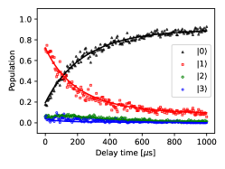
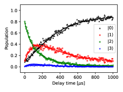
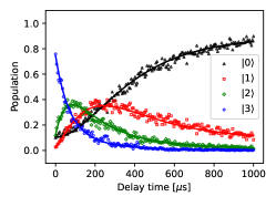
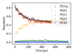
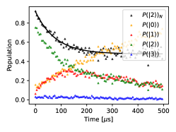
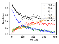
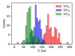
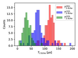
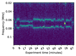
Figure 10: (a) to (c) show the population in each state as a function of the waiting time, when the transmon is initially prepared in the $\ket{1}$, $\ket{2}$, $\ket{3}$ state, respectively. (d) to (f) shows a typical result Spin Echo experiment performed on the $\{\ket{0},\ket{1}\}$, $\{\ket{1},\ket{2}\}$, $\{\ket{2},\ket{3}\}$ subspaces, respectively. The black maker in these figures represents the normalized success rate $P=P(\ket{i+1})/(P(\ket{i})+P(\ket{i+1}))$, which is used to reduce the impact of the decay of the transmon during the experiment. (g) and (h) show the distribution of the effective $T_{1}$ and $T_{2}$ echo times, respectively, with repeated measurements. These experiments are repeated for 100 times. (i) displays the Fourier spectrum of the trace of the Ramsey interferometry experiment performed on the $\{\ket{2},\ket{3}\}$ subspace over time. The frequency axis shows the measured frequency detuning from the transition drive frequency, while the experiment time axis denotes the time interval between the start of collecting the Ramsey trace and the start of the experiment.

To model the spontaneous decay dynamics, a matrix $\Gamma$ is employed to capture the decay rate between all energy levels Peterer et al. (2015). The state population as a function of waiting time is given by $\vec{P}(t)=e^{\Gamma t}\vec{P_{0}}$, where $\vec{P}(t)$ is the population of each state observed at time $t$, corresponding to the initial state population $\vec{P_{0}}$. The effective $T_{1}^{(ij)}=1/\Gamma_{ji}$ is then defined from the $\Gamma$ matrix, where $i$ and $j$ are the neighboring energy levels. The transmon is reported to have $T_{1}^{(01)}=189\pm 41~{}\mathrm{\mu s}$, $T_{1}^{(12)}=119\pm 21~{}\mathrm{\mu s}$, and $T_{1}^{(23)}=87\pm 23~{}\mathrm{\mu s}$. To characterize the dephasing dynamics, spin echo experiments are performed on each neighbouring subspace to determine $T_{2}$, which describes the phase coherence of the subspace. The normalized survival population $P(\ket{i})N$ is defined as $P(\ket{i})_{N}=P(i)/(P(i)+P(i-1))$ to remove the effect of energy relaxation, where $P(\ket{i})$ is the population ratio measured in state $\ket{i}$ with $i>0$. $P(\ket{i})_{N}$ is fitted to $P(\ket{i})_{N}(t)=e^{-t/T_{2}^{(i)}}P(\ket{i})_{N}(0)$, where $T_{2}^{(i)}$ is the effective $T_{2}$ value for the $\{\ket{i},\ket{i-1}\}$ subspace. The experimentally determined transmon parameters are $T_{2}^{(01)}=118\pm 21\mathrm{~{}\mu s}$, $T_{2}^{(12)}=76\pm 27\mathrm{~{}\mu s}$, and $T_{2}^{(23)}=35\pm 14\mathrm{~{}\mu s}$.

The charge-noise-induced error on the higher levels can be a problem for executing quantum algorithms. To measure the sensitivity of the charge noise, we implement a Ramsey interferometry experiment on the ${\ket{2},\ket{3}}$ subspace, as it is the most sensitive subspace among all three neighbouring subspaces of the four lowest transmon levels Tennant et al. (2022); Martinez et al. (2022). Our results show that the frequency shift due to charge noise is around $20\mathrm{~{}kHz}$, which is significantly lower than the rabi rate of a single qudit pulse (which is $20$ MHz for a $50$ ns long $\pi$ pulse). This implies that the charge noise contribution to the error would not be detrimental to the implementation of quantum algorithms.

Appendix D Gate set tomography

Gate Set Tomography (GST) is one of the protocols for Quantum Characterisation, Verification and Validation (QCVV). GST performs process tomography for the full gate set, and estimates the state preparation and measurement (SPAM) error while reconstruct the CPTP map of the quantum operations Greenbaum (2015); Nielsen et al. (2021). To implement gate-set tomography on the qudit system, we need to define the Preparation and measurement fiducials to span the whole Hilbert space. The fiducials are simply the two-qubit fiducials mapped to the qudit native, gates, given in Tab.2. The tomography result of the gate set is shown in Fig.11.

Table 2: Fiducials for qudit gate set tomography. These fiducials are the two-qubit fiducials to mapped to the qudit, and can be straightforwardly implemented on the emulator.

Preparation Fiducials ($F^{(p)}$)
1	$I$
2	$X_{01}(\frac{\pi}{2})$
3	$X_{01}(\frac{\pi}{2}).Z_{1}(\frac{\pi}{2})$
4	$X_{01}(\frac{\pi}{2}).X_{01}(\frac{\pi}{2})$
5	$X_{01}(\frac{\pi}{2}).X_{01}(\frac{\pi}{2}).X_{12}(\frac{\pi}{2})$
6	$X_{01}(\frac{\pi}{2}).X_{01}(\frac{\pi}{2}).X_{12}(\frac{\pi}{2}).Z_{2}(\frac{\pi}{2})$
7	$X_{01}(\frac{\pi}{2}).X_{12}(\frac{\pi}{2}).X_{12}(\frac{\pi}{2})$
8	$X_{01}(\frac{\pi}{2}).Z_{1}(\frac{\pi}{2}).X_{12}(\frac{\pi}{2}).X_{12}(\frac{\pi}{2})$
9	$X_{01}(\frac{\pi}{2}).X_{01}(\frac{\pi}{2}).X_{12}(\frac{\pi}{2}).X_{12}(\frac{\pi}{2})$
10	$X_{01}(\frac{\pi}{2}).X_{12}(\frac{\pi}{2}).X_{12}(\frac{\pi}{2}).X_{23}(\frac{\pi}{2}).X_{23}(\frac{\pi}{2})$
11	$X_{01}(\frac{\pi}{2}).Z_{1}(\frac{\pi}{2}).X_{12}(\frac{\pi}{2}).X_{12}(\frac{\pi}{2}).X_{23}(\frac{\pi}{2}).X_{23}(\frac{\pi}{2})$
12	$X_{01}(\frac{\pi}{2}).X_{01}(\frac{\pi}{2}).X_{12}(\frac{\pi}{2}).X_{23}(\frac{\pi}{2}).X_{23}(\frac{\pi}{2})$
13	$X_{01}(\frac{\pi}{2}).X_{01}(\frac{\pi}{2}).X_{12}(\frac{\pi}{2}).Z_{2}(\frac{\pi}{2}).X_{23}(\frac{\pi}{2}).X_{23}(\frac{\pi}{2})$
14	$X_{01}(\frac{\pi}{2}).X_{01}(\frac{\pi}{2}).X_{12}(\frac{\pi}{2}).X_{12}(\frac{\pi}{2}).X_{23}(\frac{\pi}{2})$
15	$X_{01}(\frac{\pi}{2}).X_{01}(\frac{\pi}{2}).X_{12}(\frac{\pi}{2}).X_{12}(\frac{\pi}{2}).X_{23}(\frac{\pi}{2}).Z_{3}(\frac{\pi}{2})$
16	$X_{01}(\frac{\pi}{2}).X_{01}(\frac{\pi}{2}).X_{12}(\frac{\pi}{2}).X_{12}(\frac{\pi}{2}).X_{23}(\frac{\pi}{2}).X_{23}(\frac{\pi}{2})$
Measurement Fiducials($F^{(m)}$)
1	$I$
2	$Z_{1}(\frac{\pi}{2}).Z_{3}(\frac{\pi}{2}).X_{01}(\frac{\pi}{2}).X_{23}(\frac{\pi}{2})$
3	$X_{01}(\frac{\pi}{2}).X_{23}(\frac{\pi}{2})$
4	$X_{12}(\frac{\pi}{2}).X_{12}(\frac{\pi}{2}).Z_{1}(\frac{\pi}{2}).Z_{2}(\frac{\pi}{2}).Z_{1}(\frac{\pi}{2}).Z_{3}(\frac{\pi}{2}).X_{01}(\frac{\pi}{2}).X_{23}(\frac{\pi}{2}).$
	$X_{12}(\frac{\pi}{2}).X_{12}(\frac{\pi}{2}).Z_{1}(\frac{\pi}{2}).Z_{2}(\frac{\pi}{2})$
5	$X_{12}(\frac{\pi}{2}).X_{12}(\frac{\pi}{2}).Z_{1}(\frac{\pi}{2}).Z_{2}(\frac{\pi}{2}).Z_{1}(\frac{\pi}{2}).Z_{3}(\frac{\pi}{2}).X_{01}(\frac{\pi}{2}).X_{23}(\frac{\pi}{2}).$
	$X_{12}(\frac{\pi}{2}).X_{12}(\frac{\pi}{2}).Z_{1}(\frac{\pi}{2}).Z_{2}(\frac{\pi}{2}).Z_{1}(\frac{\pi}{2}).Z_{3}(\frac{\pi}{2}).X_{01}(\frac{\pi}{2}).X_{23}(\frac{\pi}{2})$
6	$X_{12}(\frac{\pi}{2}).X_{12}(\frac{\pi}{2}).Z_{1}(\frac{\pi}{2}).Z_{2}(\frac{\pi}{2}).Z_{1}(\frac{\pi}{2}).Z_{3}(\frac{\pi}{2}).X_{01}(\frac{\pi}{2}).X_{23}(\frac{\pi}{2}).$
	$X_{12}(\frac{\pi}{2}).X_{12}(\frac{\pi}{2}).Z_{1}(\frac{\pi}{2}).Z_{2}(\frac{\pi}{2}).X_{01}(\frac{\pi}{2}).X_{23}(\frac{\pi}{2})$
7	$X_{12}(\frac{\pi}{2}).X_{12}(\frac{\pi}{2}).Z_{1}(\frac{\pi}{2}).Z_{2}(\frac{\pi}{2}).X_{01}(\frac{\pi}{2}).X_{23}(\frac{\pi}{2}).X_{12}(\frac{\pi}{2}).X_{12}(\frac{\pi}{2}).$
	$Z_{1}(\frac{\pi}{2}).Z_{2}(\frac{\pi}{2})$
8	$X_{12}(\frac{\pi}{2}).X_{12}(\frac{\pi}{2}).Z_{1}(\frac{\pi}{2}).Z_{2}(\frac{\pi}{2}).X_{01}(\frac{\pi}{2}).X_{23}(\frac{\pi}{2}).X_{12}(\frac{\pi}{2}).X_{12}(\frac{\pi}{2}).$
	$Z_{1}(\frac{\pi}{2}).Z_{2}(\frac{\pi}{2}).Z_{1}(\frac{\pi}{2}).Z_{3}(\frac{\pi}{2}).X_{01}(\frac{\pi}{2}).X_{23}(\frac{\pi}{2})$
9	$X_{12}(\frac{\pi}{2}).X_{12}(\frac{\pi}{2}).Z_{1}(\frac{\pi}{2}).Z_{2}(\frac{\pi}{2}).X_{01}(\frac{\pi}{2}).X_{23}(\frac{\pi}{2}).X_{12}(\frac{\pi}{2}).X_{12}(\frac{\pi}{2}).$
	$Z_{1}(\frac{\pi}{2}).Z_{2}(\frac{\pi}{2}).X_{01}(\frac{\pi}{2}).X_{23}(\frac{\pi}{2})$

We found the estimated gate fidelity for the $\{\ket{0},\ket{1}\}$ subspace is lower than $\{\ket{1},\ket{2}\}$ and $\{\ket{2},\ket{3}\}$ subspace, despite it has better coherence. The control pulses RF signal is generated by mixing an IF signal generated by a 2 Gsps DAC and a fixed LO signal. The LO frequency is selected as 3.904 GHz to cover the transition frequencies of the qubit states $\{\ket{0},\ket{1}\}$, $\{\ket{1},\ket{2}\}$, and $\{\ket{2},\ket{3}\}$. This choice of LO frequency results in an IF frequency of 230 MHz for the $\{\ket{0},\ket{1}\}$ transition, which is at the upper limit of our DAC’s frequency bandwidth. Therefore, we hypothesize that this could be a contributing factor to the lower gate fidelity observed in the $\{\ket{0},\ket{1}\}$ subspace compared to the $\{\ket{1},\ket{2}\}$ and $\{\ket{2},\ket{3}\}$ subspace.

Gate name	$X_{01}(\frac{\pi}{2})$	$X_{12}(\frac{\pi}{2})$	$X_{23}(\frac{\pi}{2})$
Average infidelity	$0.00498(11)$	$0.002966(52)$	$0.002906(68)$
PTM
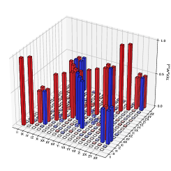
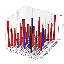
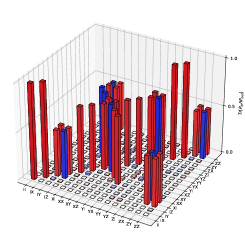
Error generator
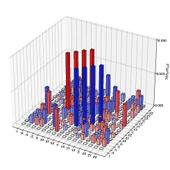
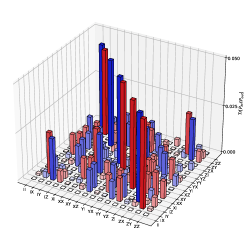
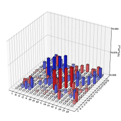
Gate name	$Z_{1}(\frac{\pi}{2})$	$Z_{2}(\frac{\pi}{2})$	$Z_{3}(\frac{\pi}{2})$
Average infidelity	$0.000085(15)$	$0.000218(70)$	$0.000113(80)$
PTM
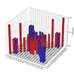
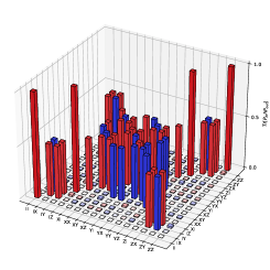
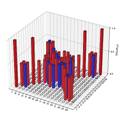
Error Generator

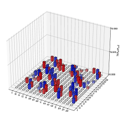
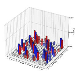
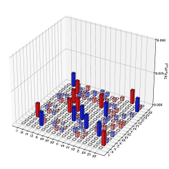
Figure 11: Averaged gate infidelities, reconstructed process matrix and error generators of the gate set. The result is generated by pyGSTi maximum likelihood estimation.

References

Nielsen and Chuang (2000)Michael A. Nielsen and Isaac L. Chuang, Quantum
computation and quantum information (Cambridge
University Press, 2000) p. 676.
TAMATE et al. (2022)Shuhei TAMATE, Yutaka TABUCHI, and Yasunobu NAKAMURA, “Toward
Realization of Scalable Packaging and Wiring for Large-Scale Superconducting
Quantum Computers,” IEICE Transactions on
Electronics E105.C, 2021SEP0007 (2022).
Stefanazzi et al. (2022)Leandro Stefanazzi, Kenneth Treptow, Neal Wilcer,
Chris Stoughton, Collin Bradford, Sho Uemura, Silvia Zorzetti, Salvatore Montella, Gustavo Cancelo, Sara Sussman, Andrew Houck, Shefali Saxena, Horacio Arnaldi, Ankur Agrawal, Helin Zhang, Chunyang Ding, and David I. Schuster, “The QICK (Quantum Instrumentation Control Kit):
Readout and control for qubits and detectors,” Review of
Scientific Instruments 93, 044709 (2022).
Theis et al. (2016)L. S. Theis, F. Motzoi, and F. K. Wilhelm, “Simultaneous gates in
frequency-crowded multilevel systems using fast, robust, analytic control
shapes,” Physical Review A 93, 012324 (2016).
Schutjens et al. (2013)R. Schutjens, F. Abu Dagga, D. J. Egger, and F. K. Wilhelm, “Single-qubit gates in
frequency-crowded transmon systems,” Physical Review A 88, 052330 (2013).
Slussarenko and Pryde (2019)Sergei Slussarenko and Geoff J. Pryde, “Photonic quantum information processing: A concise review,” Applied Physics Reviews 6, 041303 (2019).
Fickler et al. (2012)Robert Fickler, Radek Lapkiewicz, William N. Plick, Mario Krenn,
Christoph Schaeff,
Sven Ramelow, and Anton Zeilinger, “Quantum entanglement of
high angular momenta,” Science 338, 640–643 (2012).
Malik et al. (2016)Mehul Malik, Manuel Erhard,
Marcus Huber, Mario Krenn, Robert Fickler, and Anton Zeilinger, “Multi-photon entanglement in high
dimensions,” Nature Photonics 2016 10:4 10, 248–252 (2016).
Wang et al. (2018)Jianwei Wang, Stefano Paesani,
Yunhong Ding, Raffaele Santagati, Paul Skrzypczyk, Alexia Salavrakos, Jordi Tura, Remigiusz Augusiak, Laura Mančinska, Davide Bacco, Damien Bonneau, Joshua W. Silverstone, Qihuang Gong, Antonio Acín, Karsten Rottwitt, Leif K. Oxenløwe, Jeremy L. O’Brien, Anthony Laing, and Mark G. Thompson, “Multidimensional quantum entanglement with
large-scale integrated optics,” Science 360, 285–291 (2018).
Lu et al. (2020)Hsuan‐Hao Lu, Zixuan Hu, Mohammed Saleh Alshaykh, Alexandria Jeanine Moore, Yuchen Wang, Poolad Imany, Andrew Marc Weiner, and Sabre Kais, “Quantum Phase
Estimation with Time‐Frequency Qudits in a Single Photon,” Advanced Quantum Technologies 3, 1900074 (2020).
Kues et al. (2017)Michael Kues, Christian Reimer, Piotr Roztocki, Luis Romero Cortés, Stefania Sciara, Benjamin Wetzel, Yanbing Zhang,
Alfonso Cino, Sai T. Chu, Brent E. Little, David J. Moss, Lucia Caspani, José Azaña, and Roberto Morandotti, “On-chip generation of high-dimensional
entangled quantum states and their coherent control,” Nature 2017
546:7660 546, 622–626
(2017).
Bruzewicz et al. (2019)Colin D. Bruzewicz, John Chiaverini, Robert McConnell, and Jeremy M. Sage, “Trapped-ion quantum computing: Progress and challenges,” Applied Physics Reviews 6, 021314 (2019).
Ringbauer et al. (2022)Martin Ringbauer, Michael Meth, Lukas Postler,
Roman Stricker, Rainer Blatt, Philipp Schindler, and Thomas Monz, “A universal qudit quantum processor with trapped
ions,” Nature Physics 18, 1053–1057 (2022).
Dogra et al. (2014)Shruti Dogra, Arvind, and Kavita Dorai, “Determining the parity of a permutation using
an experimental NMR qutrit,” Physics Letters A 378, 3452–3456 (2014).
Dogra et al. (2016)Shruti Dogra, Kavita Dorai, and Arvind, “Experimental demonstration of quantum
contextuality on an NMR qutrit,” Physics Letters A 380, 1941–1946 (2016).
Gedik et al. (2015)Z. Gedik, I. A. Silva,
B. Çakmak, G. Karpat, E. L. G. Vidoto, D. O. Soares-Pinto, E. R. deAzevedo, and F. F. Fanchini, “Computational speed-up with a single qudit,” Scientific Reports 5, 14671 (2015).
Krantz et al. (2019)P. Krantz, M. Kjaergaard,
F. Yan, T. P. Orlando, S. Gustavsson, and W. D. Oliver, “A quantum engineer’s guide to superconducting
qubits,” Applied Physics Reviews 6, 021318 (2019).
Wallquist et al. (2009)M Wallquist, K Hammerer,
P Rabl, S M Girvin, M H Devoret, and R J Schoelkopf, “Circuit QED and engineering charge-based
superconducting qubits,” Physica Scripta 2009, 014012 (2009).
Koch et al. (2007)Jens Koch, Terri M. Yu,
Jay Gambetta, A. A. Houck, D. I. Schuster, J. Majer, Alexandre Blais, M. H. Devoret, S. M. Girvin, and R. J. Schoelkopf, “Charge-insensitive qubit design derived from the Cooper pair box,” Physical Review A - Atomic, Molecular, and Optical Physics 76, 1–21 (2007).
Peterer et al. (2015)Michael J. Peterer, Samuel J. Bader, Xiaoyue Jin, Fei Yan, Archana Kamal,
Theodore J. Gudmundsen,
Peter J. Leek, Terry P. Orlando, William D. Oliver, and Simon Gustavsson, “Coherence and decay of higher energy
levels of a superconducting transmon qubit,” Physical Review Letters 114, 010501 (2015).
Bianchetti et al. (2010)R. Bianchetti, S. Filipp,
M. Baur, J. M. Fink, C. Lang, L. Steffen, M. Boissonneault, A. Blais, and A. Wallraff, “Control and Tomography of a Three Level Superconducting Artificial
Atom,” Physical Review Letters 105, 223601 (2010).
Dong et al. (2022)Yuqian Dong, Qiang Liu,
Jianhua Wang, Qingshi Li, Xiaoyan Yu, Wen Zheng, Yong Li, Dong Lan, Xinsheng Tan, and Yang Yu, “Simulation of Two-Qubit Gates with a Superconducting Qudit,” physica status solidi (b) 259, 2100500 (2022).
Tan et al. (2018)Xinsheng Tan, Dan Wei Zhang, Qiang Liu,
Guangming Xue, Hai Feng Yu, Yan Qing Zhu, Hui Yan, Shi Liang Zhu, and Yang Yu, “Topological Maxwell Metal Bands in a Superconducting Qutrit,” Physical Review Letters 120, 130503 (2018).
Blok et al. (2021)M. S. Blok, V. V. Ramasesh,
T. Schuster, K. O’Brien, J. M. Kreikebaum, D. Dahlen, A. Morvan, B. Yoshida, N. Y. Yao, and I. Siddiqi, “Quantum Information Scrambling on a Superconducting Qutrit
Processor,” Physical Review X 11, 021010 (2021).
Tan et al. (2021)Xinsheng Tan, Dan Wei Zhang, Wen Zheng,
Xiaopei Yang, Shuqing Song, Zhikun Han, Yuqian Dong, Zhimin Wang, Dong Lan, Hui Yan, Shi Liang Zhu, and Yang Yu, “Experimental Observation of Tensor Monopoles with a Superconducting
Qudit,” Physical Review Letters 126, 017702 (2021).
Wang et al. (2020)Yuchen Wang, Zixuan Hu,
Barry C. Sanders, and Sabre Kais, “Qudits and High-Dimensional Quantum
Computing,” Frontiers in Physics 8, 479 (2020).
Mogos (2007)Gabriela Mogos, “The
Deutsch-Josza Algorithm for n-Qudits,” in Proceedings of the 7th Conference on 7th WSEAS International
Conference on Applied Computer Science - Volume 7 (2007) pp. 49–51.
Krishna et al. (2016)Rajath Krishna, Vishesh Makwana, and Ananda Padhmanabhan Suresh, “A
Generalization of Bernstein-Vazirani Algorithm to Qudit Systems,” (2016).
Ivanov et al. (2012)S. S. Ivanov, H. S. Tonchev,
and N. V. Vitanov, “Time-efficient
implementation of quantum search with qudits,” Physical Review A 85, 062321 (2012).
Pavlidis and Floratos (2021)Archimedes Pavlidis and Emmanuel Floratos, “Quantum-Fourier-transform-based quantum arithmetic with qudits,” Physical Review A 103, 032417 (2021).
Bocharov et al. (2017)Alex Bocharov, Martin Roetteler, and Krysta M. Svore, “Factoring with qutrits: Shor’s algorithm on ternary and metaplectic quantum
architectures,” Physical Review A 96, 012306 (2017).
Cerezo et al. (2021)M. Cerezo, Andrew Arrasmith, Ryan Babbush, Simon C. Benjamin, Suguru Endo,
Keisuke Fujii, Jarrod R. McClean, Kosuke Mitarai, Xiao Yuan, Lukasz Cincio, and Patrick J. Coles, “Variational quantum algorithms,” Nature Reviews Physics 2021 3:9 3, 625–644 (2021).
Tilly et al. (2021)Jules Tilly, Hongxiang Chen,
Shuxiang Cao, Dario Picozzi, Kanav Setia, Ying Li, Edward Grant, Leonard Wossnig, Ivan Rungger, George H. Booth, and Jonathan Tennyson, “The Variational Quantum Eigensolver: a review of methods and best
practices,” (2021), 10.48550/arxiv.2111.05176.
Dong et al. (2021)Yuqian Dong, Qiang Liu,
Jianhua Wang, Qingshi Li, Xiaoyan Yu, Wen Zheng, Yong Li, Dong Lan, Xinsheng Tan, and Yang Yu, “Simulation of two-qubit gates with a superconducting qudit,” physica status solidi (b) 259, 2100500 (2021).
Spring et al. (2022)Peter A. Spring, Shuxiang Cao, Takahiro Tsunoda, Giulio Campanaro, Simone Fasciati, James Wills, Mustafa Bakr, Vivek Chidambaram, Boris Shteynas, Lewis Carpenter, Paul Gow,
James Gates, Brian Vlastakis, and Peter J. Leek, “High coherence and low cross-talk in a
tileable 3d integrated superconducting circuit architecture,” Science Advances 8 (2022), 10.1126/sciadv.abl6698.
Cao et al. (2022)Shuxiang Cao, Deep Lall, Mustafa Bakr,
Giulio Campanaro,
Simone Fasciati, James Wills, Vivek Chidambaram, Boris Shteynas, Ivan Rungger, and Peter Leek, “Efficient qutrit gate-set tomography on a transmon,”
(2022), arXiv:2210.04857 .
Nielsen et al. (2020)Erik Nielsen, Kenneth Rudinger, Timothy Proctor, Antonio Russo, Kevin Young, and Robin Blume-Kohout, “Probing quantum processor
performance with pyGSTi,” Quantum Science and Technology 5, 044002 (2020).
O’Malley et al. (2016)P. J.J. O’Malley, R. Babbush,
I. D. Kivlichan, J. Romero, J. R. McClean, R. Barends, J. Kelly, P. Roushan, A. Tranter, N. Ding, B. Campbell, Y. Chen,
Z. Chen, B. Chiaro, A. Dunsworth, A. G. Fowler, E. Jeffrey, E. Lucero,
A. Megrant, J. Y. Mutus, M. Neeley, C. Neill, C. Quintana, D. Sank, A. Vainsencher, J. Wenner,
T. C. White, P. V. Coveney, P. J. Love, H. Neven, A. Aspuru-Guzik, and J. M. Martinis, “Scalable quantum simulation of molecular energies,” Physical Review X 6, 031007 (2016).
Kandala et al. (2017)Abhinav Kandala, Antonio Mezzacapo, Kristan Temme, Maika Takita,
Markus Brink, Jerry M. Chow, and Jay M. Gambetta, Nature, Tech. Rep. 7671 (2017).
Bravyi et al. (2017)Sergey Bravyi, Jay M. Gambetta, Antonio Mezzacapo, and Kristan Temme, “Tapering off qubits to
simulate fermionic hamiltonians,” (2017), arXiv:1701.08213 .
Anand et al. (2022)Abhinav Anand, Philipp Schleich, Sumner Alperin-Lea, Phillip W. K. Jensen, Sukin Sim, Manuel Díaz-Tinoco, Jakob S. Kottmann, Matthias Degroote, Artur F. Izmaylov, and Alán Aspuru-Guzik, “A quantum computing view on unitary coupled cluster
theory,” Chemical Society Reviews 51, 1659–1684 (2022).
Romero et al. (2018)Jonathan Romero, Ryan Babbush, Jarrod R McClean, Cornelius Hempel, Peter J Love,
and Alán Aspuru-Guzik, “Strategies
for quantum computing molecular energies using the unitary coupled cluster
ansatz,” Quantum Science and Technology 4, 014008 (2018).
McKay et al. (2017)David C. McKay, Christopher J. Wood, Sarah Sheldon, Jerry M. Chow, and Jay M. Gambetta, “Efficient Z
gates for quantum computing,” Physical Review A 96, 022330 (2017).
Tennant et al. (2022)Daniel M. Tennant, Luis A. Martinez, Kristin M. Beck, Sean R. O’Kelley, Christopher D. Wilen, R. McDermott, Jonathan L. Dubois, and Yaniv J. Rosen, “Low-Frequency
Correlated Charge-Noise Measurements Across Multiple Energy Transitions in a
Tantalum Transmon,” PRX Quantum 3, 030307 (2022).
Martinez et al. (2022)L. A. Martinez, Z. Peng,
D. Appelö, D. M. Tennant, N. Anders Petersson, J. L DuBois, and Y. J. Rosen, “Noise-specific beats in the higher-level Ramsey curves of
a transmon qubit,” (2022), 10.48550/arxiv.2211.06531.
Greenbaum (2015)Daniel Greenbaum, “Introduction
to Quantum Gate Set Tomography,” (2015).
Nielsen et al. (2021)Erik Nielsen, John King Gamble, Kenneth Rudinger, Travis Scholten, Kevin Young,
and Robin Blume-Kohout, “Gate Set
Tomography,” Quantum 5, 557 (2021).