Reconciling astronomical distance scales with variable red giant stars

Abstract

Stellar standard candles provide the absolute calibration for measuring the Universe’s local expansion rate, $H_{0}$, which differs by $\sim 8\%$ from the value inferred using the Cosmic Microwave Background assuming the concordance cosmological model, $\Lambda$CDM (Planck, ; Riess2022H0, ). This Hubble tension indicates a need for important revisions of fundamental physics (DiValentino2021review, ). However, the accuracy of the $H_{0}$ measurement based on classical Cepheids has been challenged by a measurement based on the Tip of the Red Giant Branch (TRGB) method (Freedman2021, ). A resolution of the Cepheids vs. TRGB dispute is needed to demonstrate well-understood systematics and to corroborate the need for new physics.

Here, we present an unprecedented $1.39\%$ absolute calibration of the TRGB distance scale based on small-amplitude red giant stars (OSARGs). Our results improve by $20\%$ upon previous calibrations and are limited by the accuracy of the distance to the Large Magellanic Cloud. This precision gain is enabled by the realization that virtually all stars at the TRGB are variable — a fact not previously exploited for TRGB calibration. Using observations and extensive simulations, we demonstrate that OSARGs yield intrinsically precise and accurate TRGB measurements thanks to the shape of their luminosity function. Inputting our calibration to the Carnegie Chicago Hubble Program’s $H_{0}$ analysis (Freedman2021, ) yields a value of $H_{0}$$=71.8\pm 1.5$ $\mathrm{km\,s^{-1}\,Mpc^{-1}}$, in $<1\sigma$ agreement with the Cepheids-based $H_{0}$ value and in $2.8\sigma$ tension with the early-Universe value.

1 Introduction

The absolute calibration of the extragalactic distance ladder (DL) is crucial to understanding the $5\sigma$ discord between recent direct measurements of the Hubble constant, $H_{0}$, and its value inferred from the Cosmic Microwave Background assuming the concordance cosmological model (Planck, ; Riess2022H0, ). The DL measures $H_{0}$ by mapping out the Hubble-Lemaître law (Lemaitre1927, ; Hubble1929, ) using the extremely precise and luminous type-Ia supernovae (SNeIa). The absolute calibration of the Hubble-Lemaître law, however, requires an intermediate step provided by stellar standard candles whose distances can be measured by geometric methods (GaiaEDR3plx, ; Pietrzynski19, ; Reid2019, ). The currently most accurate DL employs classical Cepheids to calibrate SNeIa, resulting in a $1.4\%$ measurement of $H_{0}=73.15\pm 0.97$ $\mathrm{km\,s^{-1}\,Mpc^{-1}}$ (Riess2022Clusters, ). The second most precise $H_{0}$ measurement has been obtained by calibrating SNeIa using the tip of the red giant branch (TRGB) method (Freedman2019, ; Freedman2021, ). Although most direct measurements of $H_{0}$ tend to be closer to the Cepheids-based DL (DiValentino2021review, ), the TRGB-based $H_{0}$ value reported by Freedman et al. is formally consistent with both the Cepheids and the early Universe $H_{0}$ inferred from the CMB. However, calibrations of the absolute TRGB magnitude obtained by different teams(Rizzi2007, ; Soltis2021, ; Anand2022, ; Hoyt2021, ; Freedman2021, ) differ at the level of $\sim 0.06$ mag, or roughly $1.5\sigma$, and the origins of such differences have remained somewhat unclear. Unfortunately, these differences immediately affect $H_{0}$, since the absolute magnitude of the TRGB, $M_{\mathrm{TRGB}}$, directly scales SNeIa to brighter or fainter absolute magnitudes, with a fainter $M_{\mathrm{TRGB}}$ resulting in higher $H_{0}$. Improved TRGB accuracy is therefore urgently required to understand possible differences between the Cepheids and TRGB-based $H_{0}$ measurements, with direct implications for how seriously an astrophysical solution to the Hubble discord is needed.

From an astrophysical perspective, the Tip of the Red Giant Branch is a well-understood phase of stellar evolution. In short, the Helium flash introduces a limiting luminosity for stars ascending the red giant branch for the first time, forcing them to revert direction and descend toward the Horizontal Branch prior to their further evolution (Renzini1992, ). The extremely rapid timescale of the Helium flash implies that RGB stars are always observed at somewhat lower luminosity than where the flash actually occurs. Moreover, changes in age and chemical composition lead to small differences in the absolute magnitude where the flash occurs (Salaris2005, ).

Empirically, color-magnitude diagrams (CMDs) of the LMC or the halos of other galaxies exhibit a recognizable feature that can be measured using edge detection techniques (Lee1993, ; Sakai1996, ) or maximum likelihood analyses (Mendez2002, ). The absolute magnitude of this feature can be calibrated when it is measured in regions of known distance, such as the LMC, after correcting for dust extinction. However, measuring distances ($m-M$) requires the values of $M$ to be consistent among calibrator and distant galaxies. Unfortunately, the known astrophysical differences among RGB stars (notably in age and metallicity), as well as contamination by AGB or foreground stars complicate distance measurements. Two main approaches of dealing with these complications are commonly used. The Carnegie Chicago Hubble Program (CCHP) considers the $I-$band luminosity function (LF) to be insensitive to metallicity (Madore2018, ) and selects the blue part of the RGB to select only the oldest stars (Hatt17, ; Freedman2019, ). Conversely, the Extragalactic Distance Database (EDD) team seeks to correct metallicity differences using a color term (Rizzi2007, ). Depending on the mean color of the RGB stars, both calibrations can agree (at $V-I=1.3$) or differ by $\sim 0.10$ mag (at $V-I=1.8$).

By contrast, classical Cepheids are individual standard candles because the luminosity of each star can in principle be calibrated using direct parallax measurements. Stars near the TRGB, however, are commonly considered to be non-variable for purposes of measuring the tip. This prompted us to investigate how variability of RGB stars could a) improve sample homogeneity, b) increase TRGB contrast, and c) otherwise help to improve the TRGB-based $H_{0}$ value. In the process, we found that virtually all stars near the Tip are variable, and that variable RGB stars provide more accurate $m_{\mathrm{TRGB}}$ estimates than RGB samples composed of variable and non-variable stars, cf. Section 2. This allowed us to calibrate $M_{\mathrm{TRGB}}$ to unprecedented accuracy, cf. Section 3, resulting in a value for $M_{\mathrm{F814W,syn}}$ that is consistent with the EDD calibration and supports a faster expansion rate, consistent with Cepheids, cf. Section 4. Details of our methodology, samples, data processing, and simulations are presented as Supplementary Information.

2 Methods

2.1 Every star at the TRGB is variable

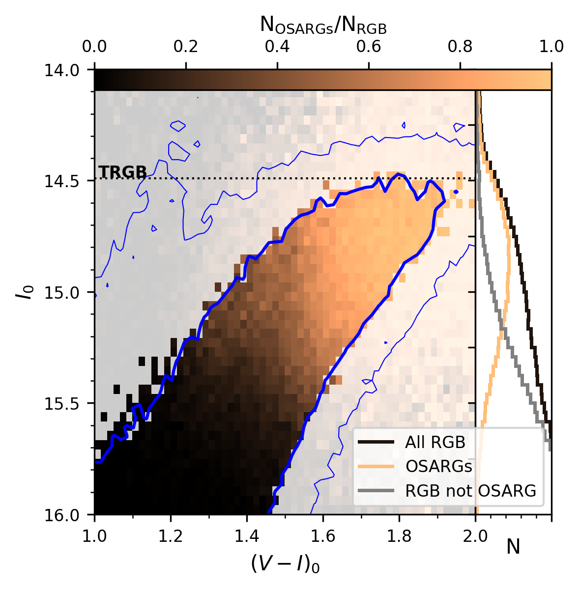
Figure 1: Virtually all stars at the TRGB are variable. Left: Coarsely-binned CMD indicating the fraction of OSARGs to all stars using a color map indicated at the top. Blue contours indicate bins with $70$ (thicker) and $20$ (thinner) of all stars in the OGLE-III photometric map of the LMC (Udalski2008, ) to highlight the location of the RGB. A rough estimate of the TRGB’s location is shown as a dotted line. The fraction of variable stars increases upward towards the TRGB, reaching nearly $100\%$ at the tip. Right: LF of RGB stars (RGBs sample, black), OSARGs (OSARGs sample, orange), and their complement (gray).

Studies targeting the TRGB for distance measurements frequently assert stars near the Tip to be non-variable. However, the variability of giant stars has been studied for a long time (Stebbins1930, ), and giant stars form multiple densely populated period-luminosity (PL) sequences (Wood1999, ). The Optical Gravitational Lensing Experiment, OGLE, enabled the discovery of a large population of small-amplitude red giants, or OSARGs (Wray2004, ), that exhibit multi-periodic variability with periods $15<P<50$ (Eyer2002, ; RedVarsIKiss2003, ; Soszynski2004, ; Soszynski09, ). Although it has been noted that multiple PL-sequences in the LMC exhibit a clear TRGB feature (RedVarsIKiss2003, ; RedVarsIIKiss2004, ), this feature has not previously been used for TRGB calibration or distance measurement.

Figure 1 shows that nearly $100\%$ of all LMC stars near the TRGB are LPVs using the OGLE-III catalogs and photometric maps (Udalski2008, ; Soszynski09, ). Selecting OSARGs should therefore yield the same $m_{\mathrm{TRGB}}$ as a selection of RGB stars. We construct two baseline samples, one following standard practice that uses all stars along the RGB (henceforth: RGBs) and the full set of OGLE-III OSARGs (Soszynski09, ) (henceforth: OSARGs). Both samples were cleaned using objective photometric quality indicators and astrometry, cf. Sects. A.2 and A.2.2. Additionally, we selected OSARGs on the A & B PL sequences (following the notation by Wood1999 ; Soszynski2004 ), which are intrinsically more homogeneous due to their similar variability, cf. A.2.2, and can be interpreted in terms of age, mass, and pulsation modes (Takayama2013, ; Wood2015, ; Trabucchi2021, ). However, we use here the A-sequence and B-sequence subsamples primarily to investigate how $m_{\mathrm{TRGB}}$ is affected when intrinsically homogeneous subgroups are selected. Moreover, we use the dispersion of their PL sequences to show that geometric corrections are not applicable to red giants in the OGLE-III LMC footprint, cf. Sect. A.5.

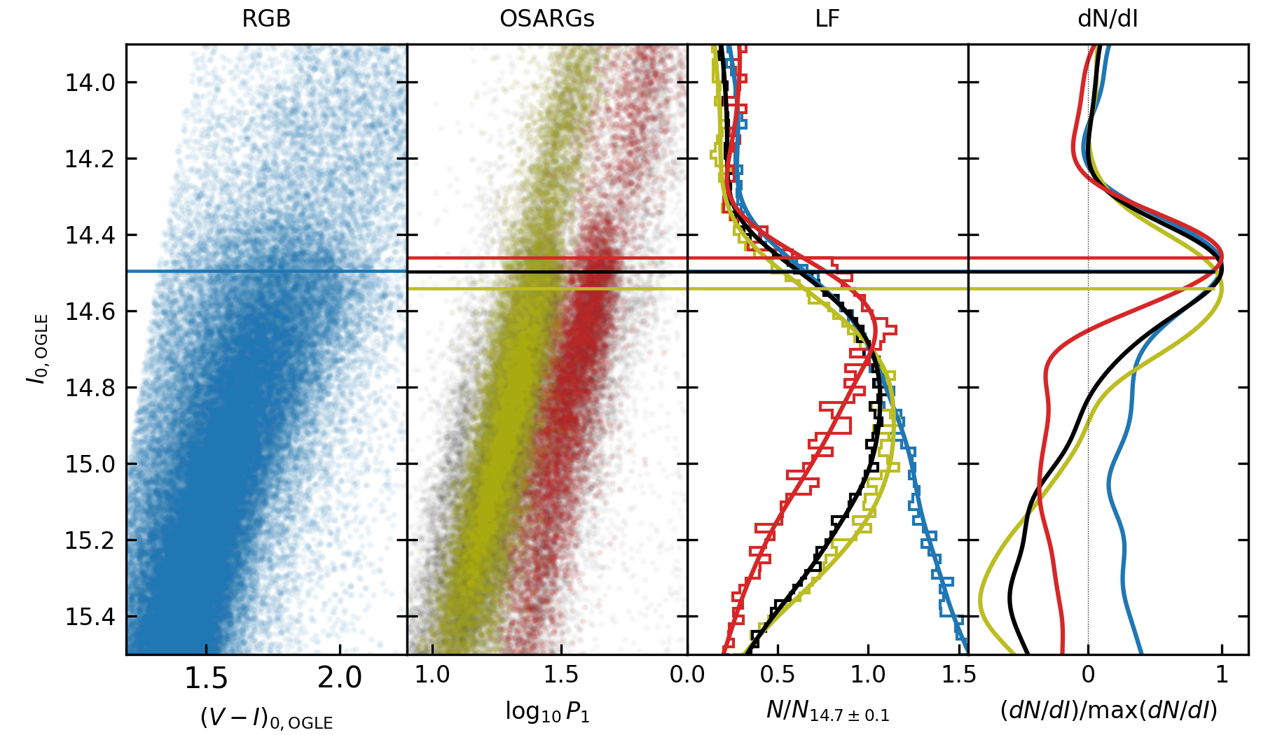
Figure 2: Illustrations of LFs and samples. Horizontal lines correspond to $m_{I,\mathrm{OGLE}}$ for the sample of identical color, with RGBs in blue, OSARGs in black, the A-sequence in yellow, and the B-sequence in red. From left to right: RGBs CMD; OSARGs PL relations zoomed in to A and B sequences; binned and smoothed LFs (here: $\sigma_{s}$$=0.15$) normalized to the number of stars with $0.1$ mag of $m_{I,\mathrm{OGLE}}$$=14.7$; Sobel edge response curves normalized to peak intensity. Normalization is used purely for visualization purposes.

2.2 Observational dataset used

We collected $V-$ and $I-$band photometric observations from OGLE-III ($m_{I,\mathrm{OGLE}}$, $m_{V,\mathrm{OGLE}}$) photometric maps (for non-variable stars) and from published time-series of LPVs. We further collected $G-$band mean magnitudes, integrated $G_{Rp}$ spectrophotometry, and synthetic photometry in Johnson-Cousins ($m_{V,\mathrm{syn}}$ and $m_{I,\mathrm{syn}}$) and HST ACS/WFC magnitudes ($m_{\mathrm{F606W,syn}}$ and $m_{\mathrm{F814W,syn}}$) based on Gaia DR3 XP spectra (Riello2021, ; Montegriffo2022, ), cf. Sect. A.1. Specifically, we used the standardized Gaia synthetic magnitudes from table gaiadr3.source (labeled GSPC) and applied residual zero-point offsets determined by Montegriffo et al. (Montegriffo2022, ) with respect to photometric standards ($\sim\pm 0.002$ mag). We added the dispersion of the calibration checks ($\sim 0.014$ mag) to the photometric uncertainties in quadrature. We applied photometric quality cuts independent of $m_{I,\mathrm{syn}}$ and removed foreground stars, cf. Sect. A.2. Comparison between $m_{I,\mathrm{OGLE}}$ and $m_{I,\mathrm{syn}}$ reveals excellent agreement to within $-0.011\pm 0.029$ mag (dispersion of $115\,975$ stars) and $-0.005\pm 0.026$ mag ($30\,315$ OSARGs). This underlines the high quality of Gaia synthetic photometry and the close agreement between the OGLE $I-$band and the reference Cousins system. Gaia’s synthetic photometry, e.g. in $m_{\mathrm{F814W,syn}}$  provides a valuable direct comparison with more distant galaxies and has been shown to agree closely with HST at magnitudes of interest to this work. Comparing $m_{I,\mathrm{OGLE}}$ to $m_{\mathrm{F814W,syn}}$, we also find excellent consistency $0.002\pm 0.028$ mag (RGBs) and $0.008\pm 0.026$ mag (OSARGs). Additional detail is presented in Sect. A.1.2.

Dust corrections are applied using OGLE reddening maps based on Red Clump standard crayons (Skowron2021ApJS, ), cf. Sect. A.6, and using a reddening law (Fitzpatrick1999, ; Schlafly2011, ) with $R_{V}=3.3$. We compute the ratio of total to selective extinction for all three $I-$bands for red giant stars near the Tip following (Anderson2022, ) and find $R_{Ic}=1.461$, $R_{\mathrm{F814W}}=1.408$. These values agree with the average value of $R_{I}$ found by (Skowron2021ApJS, , $R_{I}\sim 1.5$). However, we note the substantial difference with $R_{I}=1.219$ adopted by Hoyt2021 , which renders our $m_{I}$ values systematically brighter by $\sim 0.03$ mag with their LMC TRGB calibration for an average $E(V-I)\approx 0.12$ mag.

2.3 TRGB detection and uncertainties

We measured $m_{\mathrm{TRGB}}$ using a [-1,0,1] Sobel filter, cf. Sec. A.3, applied to a smoothed $I-$band luminosity function (LF). The Sobel filter computes the first derivative of the LF, and we associate its maximal peak (the LF inflection point) with $m_{I}$. The shape of the Sobel response function depends on both the number of stars above and below the tip and the sampling of the LF (Lee1993, ; Hatt17, ; Wu2022, ). The LF is smoothed using a GLOESS algorithm as parameterized by $\sigma_{s}$ to reduce noise (Sakai1996, ) at the penalty of introducing correlation among magnitude bins, which can bias estimates of $m_{\mathrm{TRGB}}$ (Cioni2000, ; Hatt17, ). We found that this smoothing bias, $\hat{m}_{s}$, depends on the shape of the LF in addition to $\sigma_{s}$ by measuring $m_{\mathrm{TRGB}}$ on observations for a large range of $\sigma_{s}$ values (Sect. A.3) as well as by simulated LFs (cf. Sect A.4).

We measure $m_{\mathrm{TRGB}}$ across the range of $\sigma_{s}$ values where the smoothing bias slope is shallow ($|dm_{\mathrm{TRGB}}/d\sigma_{s}|\leq 0.1$), namely $0.07\leq\sigma_{s}\leq 0.36$ for OSARGs and $0.10\leq\sigma_{s}\leq 0.15$ for RGBs. It turns out that both OSARGs and RGBs yield consistent results in these ranges, cf. Fig. 3. Using simulations (cf. Sec. A.4), we show that the reduced sensitivity to smoothing bias is a direct consequence of LF shape.

TRGB uncertainties, $\sigma_{\mathrm{MC}}$, were estimated using $1000$ Monte Carlo resamples, whereby individual magnitudes were randomly offset according to their total photometric uncertainties, $\sigma_{\mathrm{phot}}$, computed by adding in quadrature the uncertainties on mean magnitudes, $E(V-I)$, and Gaia standardization dispersion, as needed. Since smoothing reduces noise, $\sigma_{\mathrm{MC}}$ decreases with increasing $\sigma_{s}$. We therefore adopted as baseline uncertainty on $m_{I}$, $\sigma_{\mathrm{TRGB}}$, the median $\sigma_{\mathrm{MC}}$ over the $\sigma_{s}$ range where $dm_{I}/d\sigma_{s}$ is flat. This resulted in $\sigma_{\mathrm{TRGB}}$ values similar to $\sigma_{\mathrm{phot}}$ for OSARGs, and slightly larger for RGBs.

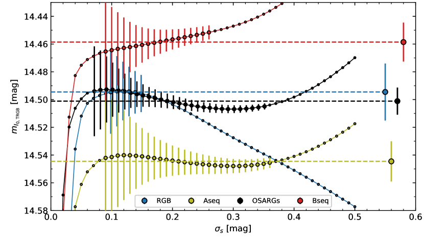
Figure 3: Dependence of $m_{I}$ on $\sigma_{s}$. Errorbars are plotted for the RGBs, OSARGs, Aseq, and Bseq samples across the range of $\sigma_{s}$ values deemed stable, which is narrow for RGBs and wide for OSARGs. Results from Tab. 1 are shown as large errorbars on the right.

3 Results

3.1 OSARGs measure the LMC TRGB to within $0.7\%$

	$\langle\mathrm{(V-I)}_{0}\rangle$	$I_{\mathrm{OGLE},0}$	$I_{\mathrm{syn},0}$	$\mathrm{F814W}_{\mathrm{syn,0}}$	$G_{{Rp},0}$	$G_{0}$
sample	(mag)	(mag)	(mag)	(mag)	(mag)	(mag)
OSARGs	$1.82\pm 0.19$	$14.501\pm 0.010$	$14.497\pm 0.011$	$14.491\pm 0.010$	$14.640\pm 0.009$	$15.621\pm 0.015$
RGBs	$1.78\pm 0.21$	$14.495\pm 0.021$	$14.478\pm 0.029$	$14.473\pm 0.027$	$14.635\pm 0.024$	$15.618\pm 0.014$
RGBs†	$1.76\pm 0.11$	$14.527\pm 0.027$	$14.506\pm 0.035$	$14.499\pm 0.032$	$14.648\pm 0.039$	$15.626\pm 0.036$
Aseq	$1.79\pm 0.15$	$14.545\pm 0.013$	$14.543\pm 0.012$	$14.537\pm 0.012$	$14.690\pm 0.009$	$15.655\pm 0.016$
Bseq	$1.82\pm 0.19$	$14.459\pm 0.014$	$14.457\pm 0.015$	$14.452\pm 0.013$	$14.607\pm 0.013$	$15.566\pm 0.030$

Table 1: TRGB apparent magnitudes in the LMC, corrected for extinction. $I_{\mathrm{syn},0}$ and $\mathrm{F814W}_{\mathrm{syn,0}}$ denote synthetic photometry based on Gaia DR3 XP spectra (Sect. A.1.2). $G_{{Rp},0}$ and $G_{0}$ are integrated spectrophotometric and white-light magnitudes from Gaia. Results reported are the median across $|dm_{\mathrm{TRGB}}/d\sigma_{s}|\leq 0.1$ range. Uncertainties combine in quadrature the median MC error, $m_{\mathrm{TRGB}}$ dispersion, and the dispersion of the difference between $m_{\mathrm{TRGB}}$ values determined as means and medians from the MC samples. An additional systematic uncertainty of $\pm 0.010$ mag applies and is estimated from simulations (cf. Sect. A.4). Median $\mathrm{(V-I)_{0}}$ colors within $\pm 0.10$ mag of $m_{\mathrm{TRGB}}$ are reported with the $16-84$ percentile range. ^†: color cut as in Hoyt2021 .

Table 1 lists our results for the RGBs and OSARGs samples, also illustrated in Fig. 3, and for two comparison samples in several de-reddened pass-bands. The most accurate—precise and bias-free—result is obtained using the OSARGs sample, consistent with expectations based on our simulations. Our central values and uncertainties on $m_{\mathrm{TRGB}}$ are obtained by considering results across the range where $|dm_{I}/d\sigma_{s}|\leq 0.1$. Center values correspond to the median $m_{\mathrm{TRGB}}$ in this range, and uncertainties sum in quadrature the median MC error, dispersion in $m_{I}$, and the dispersion of the difference between mean and median TRGB magnitudes. We stress that the MC errors already include the (dominant) contribution of reddening uncertainties and systematics, as well as standardization of Gaia synthetic magnitudes, resulting in an average de-reddened magnitude uncertainty of $0.088$ mag. The significantly improved uncertainties of the OSARGs sample compared to RGBs are driven by the insensitivity to smoothing bias, which allows us to benefit from reduced noise at higher smoothing without deviating from the true value. While our results for RGBs are consistent with the OSARGs results to $<0.5\sigma$, they are not competitive in terms of precision.

We find excellent agreement between all three sets of $I-$band photometry and $m_{\mathrm{F814W,syn}}$$-$$m_{I,\mathrm{syn}}$$=-0.007\pm 0.013$ mag (OSARGs), consistent with the transformation used by Freedman et al. (Freedman2019, , $-0.0069$ mag). The difference $m_{I,\mathrm{syn}}$$-$$m_{I,\mathrm{OGLE}}$$=-0.004\pm 0.013$ mag matches the mean difference found for all $30315$ OSARGs stars ($-0.005$ mag, cf. Sec. 2.2). These comparisons both underline the accuracy of Gaia DR3 synthetic photometry and corroborate the applicability of our $m_{I,\mathrm{syn}}$ and $m_{\mathrm{F814W,syn}}$ measurements for extragalactic distance estimation using HST photometry.

A total systematic uncertainty of $0.010$ mag is estimated using simulations (cf. Sect. A.4) and variations of bin size and phase (cf. Sect. A.3). Reddening uncertainties are already included in the MC uncertainties.

Our baseline result for DL-related discussion is $m_{\mathrm{F814W,syn}}$$=14.491\pm 0.010(\mathrm{stat})\pm 0.010(\mathrm{syst})$ mag. We did not perform color-cuts on this sample to ensure compatibility with the CCHP DL Freedman2019 ; Freedman2021 , resulting in $(V-I)_{0}=1.82\pm 0.19$ (median with $16-84\%$ percentile range) within $\pm 0.1$ mag of the Tip. Applying the color selection by Hoyt2021 results in $(V-I)_{0}=1.76\pm 0.11$ mag, removing both the bluest and reddest part of the RGB and resulting in $m_{\mathrm{F814W,syn}}$ fainter by $+0.026$ mag. We did not apply geometric corrections, since this would increase the observed PL-relation dispersion of OSARGs, cf. Sect. A.5. However, we note that geometric corrections from the literature have an irrelevant effect on our results, brightening $m_{\mathrm{TRGB}}$ values by $\sim 5$ mmag.

3.2 A $1.4\%$ calibration of the TRGB distance scale

Using the known geometric distance to the LMC based on detached eclipsing binaries (Pietrzynski19, , $\mu=18.477\pm 0.006(\mathrm{stat})\pm 0.026(\mathrm{syst})$), we obtain the most accurate absolute calibration of the $I-$band TRGB absolute luminosity to date: $M_{\mathrm{F814W,syn}}$$=-3.986\pm 0.011(\mathrm{stat})$ mag, $M_{I,\mathrm{syn}}$$=-3.979\pm 0.011(\mathrm{stat})$ mag, and $M_{I,\mathrm{OGLE}}$$=-3.975\pm 0.010(\mathrm{stat})$ mag. Adding systematic uncertainties in quadrature yields $0.028$ mag and dominates the combined uncertainty of $0.030$ mag, or $1.3\%$ in distance.

Our result differs significantly from $M_{I}=-4.049\pm 0.015(\mathrm{stat})\pm 0.035(\mathrm{syst})$ mag (at $(V-I)_{0}=1.6$ mag) used by the CCHP (Freedman2021, , an average over the LMC, SMC, and Milky Way globular clusters), as well as from their baseline LMC calibration specifically $M_{I}=-4.038\pm 0.012(\mathrm{stat})\pm 0.032(\mathrm{syst})$ (Hoyt2021, , their flat TRGB calibration). While this is in the range of discrepancies seen in the recent literature (Freedman2021, ; Anand2022, ), we trace a $0.029$ mag difference to an inadequate value of $R_{I}=1.219$ used by Hoyt2021 , cf. Sect. A.6. The remaining difference may be explained by the selection of ranked fields by Hoyt2021 , since their result for the full LMC matches our RGBs result (their Tab. 5, $m_{I}$$=14.498\pm 0.052$ mag matches our $14.527-0.030=14.497$ mag) when the same color cut is applied and the reddening difference is considered. Given the overlap in OGLE photometry and reddening maps, this agreement is not surprising. However, we find fully consistent results also using the independent Gaia data. Moreover, we found even larger differences ($\pm 0.04-0.05$ mag) by selecting intrinsically more homogeneous stellar samples (Aseq, Bseq samples) using variability information alone (no spatial selection applied). While Hoyt2021 interpreted such differences in terms of local star formation history, we note that variable star selections producing such differences are distributed throughout the LMC and not restricted to specific locations.

Conversely, our result agrees with other literature calibrations, including that used by the EDD team (Rizzi2007, ), which independently of the LMC and predicts $M_{I,\mathrm{syn}}$$=-4.00\pm 0.03$ mag at our OSARGs mean color of $(V-I)_{0}=1.82$ mag. Our calibration also matches that based on Gaia parallaxes of $\omega$ Centauri (Soltis2021, ), as well as the LMC estimate reported therein, and NGC 4258 (Reid2019, ).

We caution that striving for sample homogeneity during TRGB calibrations likely introduces distance bias because of the inability to perform analogous selections at greater distances due to lack of observational information. We therefore adopt the full OSARGs sample for our baseline result. Insensitivity to smoothing bias (cf. Sect. A.3), better contrast, and greater TRGB steepness (cf. Sect. A.4) render this sample superior to the RGBs sample without loss of stars near the TRGB, cf. Fig. 1.

3.3 Reconciling TRGB and Cepheid distance scales

It is enticing to propagate our unprecedented calibration of $M_{\mathrm{F814W,syn}}$ to estimate the value of $H_{0}$. Using the LMC as the sole anchor and information provided by the CCHP (Freedman2021, , their tables 3, 5 & 6), we estimate $H_{0}$ using TRGB observations in SN-host galaxies and the CSP-I SNeIa sample (CSP, ). Given a $2.9\%$ increase in TRGB distances implied by our calibration results in the same increase in $H_{0}$, while the reduction in the calibration uncertainty sharpens the zero-point uncertainty from $1.75\%$ to $1.39\%$. Thus, we obtain $H_{0}=71.8\pm 1.5$ $\mathrm{km\,s^{-1}\,Mpc^{-1}}$, where we have added statistical and systematic uncertainties in quadrature. Combining instead our LMC calibration with other host galaxies and computing weighted averages and weighted mean uncertainties yields $\langle$ $M_{\mathrm{F814W,syn}}$$\rangle$ $=-4.013\pm 0.022$ (NGC4258 as in JangLee17 , SMC (Hoyt2021CCHP, ), and Milky Way Globular Clusters (Cerny2020, ) as in Freedman2021 ), $-4.001\pm 0.020$ (replacing NGC4258 with Reid2019 and Cerny2020 with Soltis2021 ), and $-3.994\pm 0.023$ mag using the two most precise anchors (NGC4258 Reid2019 , our LMC). These average $M_{\mathrm{F814W,syn}}$ values are consistent with each other and would give $H_{0}$$=71.0$, $71.4$, and $71.6$ $\mathrm{km\,s^{-1}\,Mpc^{-1}}$, respectively. Our $H_{0}$ estimate agrees within $0.7\sigma$ of the one determined by the SH0ES and Pantheon+ teams (Riess2022H0, ; Brout2022, ; Scolnic2022, ; Yuan2022, ) and reconciles the dispute among the most precise stellar standard candles. Moreover, this value differs by $2.8\sigma$ from the early Universe $H_{0}$ value inferred by Planck assuming $\Lambda$CDM.

4 Conclusions

We have shown that virtually all stars near the TRGB exhibit OSARG variability. This is a feature of RGB stars, which become more variable at higher luminosity. The OSARGs LF is superior to the RGB star LF for TRGB calibration as it yields the most precise and accurate values of $m_{\mathrm{F814W,syn}}$$=14.491\pm 0.010$ mag. Using OSARG subsamples selected using variability properties (not spatially), we find differences of $0.041$ and $-0.046$ mag relative to the OSARGs sample, and a difference of $\Delta$ $m_{\mathrm{F814W,syn}}$$=0.087\pm 0.017$ mag ($5.1\sigma$) between the A and B OSARG sequences. While astrophysically pure samples enable extremely precise $m_{\mathrm{TRGB}}$ measurements thanks to improved TRGB contrast, we caution that calibrating $M_{\mathrm{TRGB}}$ using astrophysically homogeneous samples introduces systematic differences with the observed mixed RGB populations of more distant galaxies. However, OSARG variability — if detectable — could shed further light into variations of $m_{\mathrm{TRGB}}$ across multiple halo fields of the same galaxy, cf. Wu2022 .

Using the known LMC distance, we calibrate $M_{\mathrm{F814W,syn}}$= $-3.986\pm 0.011\ (\mathrm{stat})\pm 0.028\ (\mathrm{syst})$ mag to within $1.4\%$. This value agrees well with several recent literature calibrations (Rizzi2007, ; Soltis2021, ; Reid2019, ), while it disagrees by $\sim 0.063$ mag ($2.9\%)$ from the calibration used by the CCHP (Freedman2021, ). However, the CCHP LMC calibration (Hoyt2021, ) agrees with ours if no (spatial) selections seeking greater astrophysical homogeneity are applied and a reddening systematic is corrected. Applying our calibration to the CCHP $H_{0}$ results (Freedman2021, ) yields $H_{0}$$=71.8\pm 1.5$ $\mathrm{km\,s^{-1}\,Mpc^{-1}}$, consistent with the DL calibrated using Cepheids (Riess2022H0, ) and in $2.8\sigma$ tension with the early Universe value from Planck that assumes $\Lambda$CDM. Thus, our OSARGs LMC calibration improves agreement among stellar standard candles and corroborates the need to find astrophysical solutions to the Hubble discord.

Supplementary information

This article has accompanying supplementary information in the Appendix.

Acknowledgments

RIA acknowledges funding provided by SNSF Eccellenza Professorial Fellowship PCEFP2_194638. NWK acknowledges funding through the EPFL Excellence Research Internship Program, the ThinkSwiss Research Scholarship, and the UBCO Go Global Program. The authors thank the OGLE and Gaia collaborations for producing data sets of exceptional quality without which this work would not have been possible.

Declarations

Availability of data and materials

All observational data used in this article are publicly available. OGLE-III photometric maps (Udalski2008, ) and reddening maps (Skowron2021ApJS, ) are available through the OGLE website http://ogle.astrouw.edu.pl/. Data of OSARGs (Soszynski09, ) is available through the OGLE catalog of long-period variable stars available at https://ogledb.astrouw.edu.pl/~ogle/CVS/.

Data from the ESA mission Gaia (GaiaMission, ) are available at https://gea.esac.esa.int/archive/.

Appendix A Supplementary Information

A.1 Photometric data

A.1.1 OGLE magnitudes

For the OSARGs sample, we use mean magnitudes calculated from the time series data of OGLE-III small amplitude red giants (Soszynski09, ). The low amplitudes, long baseline, and large number of observations justify the adoption of the mean and standard error on the mean, which is typically $\sim 0.001$ mag. For the RGBs sample, we use magnitudes published as part of the OGLE-III photometric maps (Udalski2008, ) that state a typical uncertainty of $0.009$ mag. In practice, the photometric uncertainties are dominated by the reddening uncertainties, cf. Sec. A.6.

A.1.2 Gaia DR3 synthetic photometry

We also considered magnitudes published as part of Gaia DR3 (Gaia21, ), including $G-$band (phot_g_mean_mag), integrated $G_{Rp}$ spectrophotometry (phot_rp_mean_mag), and magnitudes from the Gaia Synthetic Photometry Catalogue (GSPC) (Montegriffo2022, ) in Cousins $I_{c}-$band (i_jkc_mag) and HST ACS/WFC F814W (f814w_acswfc_mag). As demonstrated in the Gaia DR3 documentation (Riello2021, ; Montegriffo2022, ), GSPC photometry in the magnitude range of interest ($13<G<17$ mag) accurately reproduces the photometric standards in the Landolt and Stetson collections (JKC) and HST photometry of MW globular clusters from the HUGS project (HUGS, ) to within a couple of mmag. Based on Tabs. 2 and G.2 in Montegriffo2022 , we adopt $\Delta$ $m_{I,\mathrm{syn}}$$=0.002\pm 0.014$ mag and $\Delta$ $m_{\mathrm{F814W,syn}}$$=0.001\pm 0.017$ mag, with $\Delta=m_{\mathrm{std}}-m_{\mathrm{synth}}$ the offset between the reference system and the synthetic photometry. We note that GSPC JKC photometry has been standardized by modifying photometric transmission curves as well as background corrected, whereas transmission curves have not been altered to compute HST flight magnitudes. However, the difference between standardized and raw $I_{c}-$band photometry is less than $4$ mmag for all magnitudes and colors and most pronounced at $G<13$ mag. As noted by Montegriffo2022 , the comparison between $m_{\mathrm{F814W,syn}}$ and HUGS F814W magnitudes is somewhat hampered by crowding affecting HUGS data, rendering the dispersion of $0.017$ mag a conservative upper limit for the LMC. Differences between GSPC and “raw” Gaia XPy $m_{\mathrm{F814W,syn}}$ magnitudes are at the level of $<0.001$ mag.

We test the consistency of OGLE $I-$band photometry and the Gaia $I_{c}-$band synthetic photometry. For red giant stars in the range $12.5<I_{\mathrm{ogle}}<16.5$ mag and $1.0<V-I<2.9$ we find a mean offset and dispersion of $m_{I,\mathrm{OGLE}}$$-$$m_{I,\mathrm{syn}}$$=-0.011\pm 0.023$ mag ($N=145937$). The agreement is even better closer to the TRGB ($-0.002\pm 0.035$ mag, $N=15965$), where variability adds to the dispersion. Similar agreement at the level of $1-4$ mmag is found for the extinction-corrected TRGB measurements in Tab. 1.

A.1.3 Data selection

We used Gaia data quality indicators to clean samples from foreground objects and stars that are likely affected by blending, cf. Table 2. A selection in parallax and proper motion is applied to remove foreground stars, whereas photometric quality cuts are applied to limit exposure to blending or otherwise poor photometry, cf. Riello2021 and Montegriffo2022 .

Sample	step	$N_{\mathrm{removed}}$	$N_{\mathrm{remain}}$	$N_{\mathrm{applies}}$
	Gaia cone search (incl. color & mag cut)		540 596
	in OGLE-III footprint, have OGLE $V-$band	192 057	348 539
	Foreground stars	18 973	329 566	18 973
	LMC proper motion ellipse	1 578	327 988	20 371
	$\beta\leq 0.99$	87 322	240 666	90 386
	ipd_frac_multi_peak $<7$	7 220	233 446	31 246
	ipd_frac_odd_win $<7$	48	233 398	382
	$RUWE<1.4$	4 430	228 968	37 568
	$C^{*}<1\sigma$	60 416	168 552	147 175
	$E(V-I)\leq 0.2$	12 459	156 093	23 593
RGBs	Removing stars much bluer than RGB	15 319	140 774	43 285
RGBs†	color cuts according to Hoyt2021	24 683	116 091
	OGLE-III OSARG catalog (Soszynski09, )		79 200
	Gaia cross-match	1559	77 641
OSARGs	quality cuts as applied to RGBs	37 456	40 185
Aseq	manual selection around PL sequence A		20 470
Bseq	manual selection around PL sequence B		9 164

Table 2: Description of sample selections. Columns $N_{\mathrm{removed}}$, $N_{\mathrm{removed}}$, $N_{\mathrm{applies}}$ list the number of stars removed sequentially, the number of stars remaining in the sample after applying the cut, and the number of initial stars to which this cut applies, respectively. Foreground and proper motion cuts, as well as the photometric quality indicators are explained in the text.

Stars likely to be blended with nearby stars are removed by sequentially selecting stars with $\beta<0.99$ (cf. Sec. 9.3 in Riello2021, ), ipd_frac_multi_peak $<7$, ipd_frac_odd_win $<7$, and $C^{*}<1\sigma$ following (cf. Sec. 9.3 in Riello2021, ). The cut on $\beta$ leads to a $0.01$ mag shift in TRGB apparent magnitude, which does not vary systematically if more stringent cuts are applied. We preferred a conservative cut to avoid rejecting too many good sources. As recommended by the Gaia collaboration, we further removed stars with high RUWE $>1.4$ as systematics of the photometric processing may result in poorer astrometric quality.

Foreground stars with good Gaia EDR3 astrometry are removed if RUWE $<1.4$ and $\varpi/\sigma_{\varpi}>5$ and $\varpi-\sigma_{\varpi}>1/50000$ kpc. Stars whose proper motion deviates significantly from the LMC’s ($\left(0.511\cdot(\mu_{\alpha}^{*}-1.88)-0.697\cdot(\mu_{\delta}-0.37)\right)^{2}+\left(1.11\cdot(\mu_{\alpha}^{*}-1.88)+0.4\cdot(\mu_{\delta}-0.37)\right)^{2}<1$) (GaiaEDR3_LMC, ) with RUWE $<1.4$ were also removed.

A.2 Samples of RGB stars considered

A.2.1 RGBs: canonical RGB star selection

Our RGBs sample consists of all LMC red giant branch (RGB) stars in the OGLE-III LMC footprint cross-matched to a Gaia DR3 cone search based on the following query:

SELECT *
FROM gaiadr3.gaia_source
INNER JOIN gaiadr3.synthetic_photometry_gspc as S
ON S.source_id = gaia_source.source_id
WHERE
CONTAINS(
POINT(’ICRS’,gaiadr3.gaia_source.ra,gaiadr3.gaia_source.dec),
CIRCLE(’ICRS’,$80.9$,$-69.75$,$5.8$)
)=1
AND S.i_jkc_mag $>12.5$
AND S.i_jkc_mag $<16.5$
AND (S.v_jkc_mag - S.i_jkc_mag) $>1.0$
AND (S.v_jkc_mag - S.i_jkc_mag) $<3.5$

The cross-matched sample was cleaned by applying the quality cuts described above (Sect. A.2). Reddening corrections are applied based on Red Clump stars, cf. Sec. A.6, and stars with high extinction, $E(V-I)>0.2$, were removed from the sample to limit the impact of uncertainties on the reddening law. Finally, a simple cut to remove stars much bluer than the RGB was further applied.

For comparison with the CCHP LMC calibration (Hoyt2021, ), we perform an optional selection in magnitude and color that we refer to as RGBs^† in Tab. 1. These stars lie between the lines $a=-3\cdot((V-I)_{0}-1.6)+14.45$ and $b=-3.5\cdot((V-I)_{0}-1.95)+14.45$.

A.2.2 OGLE-III Small Amplitude Red Giants (OSARGs)

Long-period variable (LPV) stars in the LMC were first reported to exhibit a pronounced TRGB feature in the OGLE-II color magnitude diagram (Eyer2002, , their Fig. 2). The TRGB feature is also clearly seen in multiple period-luminosity (PL) sequences (Wood2000, ; RedVarsIKiss2003, ). The stellar evolutionary paths of LPV sequences are understood in some detail for PL sequences A’, A, B, C’, and C (Wood2015, ) and pulsation modes have been described (Takayama2013, ). Specifically, Sequence B corresponds to second-overtone radial pulsation (Wood2015, ). Hence, LPVs offer significant insights into stellar structure, not unlike the classical Cepheids (Bono2000, ; Anderson2016, ).

The TRGB feature is most obvious in the well-populated Sequences A and B, the latter of which exhibits the more pronounced gap above and below the tip. As noted by (RedVarsIKiss2003, ), there are tens of thousands of LPVs ($15<P<50$ d) with low photometric amplitudes ($A_{I}\lesssim 0.05$ mag) below the TRGB. Close inspection revealed that amplitude cuts are, however, not practical due to significant overlap in amplitudes between RGB and AGB stars. Although LPVs have been studied for a range of purposes, including to investigate population differences among LMC and SMC red giants (RedVarsIIKiss2004, ) and the 3D structure of the Magellanic Clouds (RedVarsIIILah2005, ), they have not previously been used to calibrate the $I-$band TRGB for extragalactic distance scale applications.

The OSARGs sample is obtained by cross-matching all $79,200$ OGLE Small Amplitude Red Giants (OSARGs) stars from OGLE-III (Soszynski09, ) with our cleaned RGBs sample. In Fig. 1 we demonstrate that nearly all stars at the TRGB are OSARGs, disproving the frequent assertion that stars near the TRGB are non-variable. All OSARGs in our catalog have three dominant periods reported, which can occur on different combinations of PL sequences. For simplicity, we selected samples Aseq and Bseq from the OSARGs sample according to whether the reported dominant period ($P_{1}$) fell on PL sequence A or B in the notation by Wood1999 , cf. Fig. 2.

A.3 TRGB detection using Sobel filters

We measure TRGB apparent magnitudes using a [-1,0,+1] Sobel filter to determine the magnitude at the LF inflection point, see e.g. Hatt17 , using a bin size of $0.002$ mag. Varying bin size and phase, we estimate a binning-related systematic uncertainty of $\pm 0.001$ mag.

Smoothing is commonly applied to LFs to reduce noise (Hatt17, ). We apply a standard Gaussian-windowed LOcal regrESSion method (GLOESS) smoothing (Persson04, ) that depends on a single variable, the smoothing parameter $\sigma_{s}$. We noticed that different GLOESS implementations in the literature (Wu2022, ) will yield different values of $\sigma_{s}$. Our implementation uses numpy polyfit (numpy, ).

We estimate the total uncertainty budget on the Sobel-filter based $m_{\mathrm{TRGB}}$ by accounting for statistical and systematic uncertainties. In particular, we repeat the same analysis for a large range of $\sigma_{s}$ values and adopt the mean value across the range where $m_{\mathrm{TRGB}}(\sigma_{s})$ changes slowly with $\sigma_{s}$, that is, where $|dm_{\mathrm{TRGB}}/d\sigma_{s}|\leq 0.1$.

Statistical uncertainties for each $m_{I}(\sigma_{s})$ are estimated via the dispersion of $1000$ Monte Carlo instances, wherein the photometry of each star in the LF is allowed to vary randomly within their uncertainties before re-measuring the TRGB. Reddening uncertainties are encapsulated within the MC uncertainties, as all magnitudes are corrected for extinction before resampling. Following Skowron2021ApJS , we also include a systematic uncertainty of $0.014$ mag. The final statistical uncertainty on $m_{\mathrm{TRGB}}$ adds in quadrature: the median MC uncertainty across the $\sigma_{s}$ range considered, the dispersion of $m_{I}$ values across this range, and the dispersion of the differences between $m_{I}(\sigma_{s})$ calculated using the mean or the median. The largest contributor to the statistical uncertainty is the median MC dispersion. We found that bootstrap resampling yield dispersions smaller by about $1/3$. However, we here opt for MC dispersion as they allow for a straightforward inclusion of uncertainties associated with extinction.

A.4 LF simulations

We performed extensive simulations to investigate systematics affecting the TRGB measurement of the OSARGs and RGBs samples. We adopted an analytic representation that provides a close match to observed LFs while allowing for straightforward variations to be explored. The LFs was composed of three components: a) an AGB population ($A(m)$) modeled as a Gaussian of height $a_{\mathrm{AGB}}$, dispersion $\sigma_{\mathrm{AGB}}$, and mean computed as an offset $\Delta m_{\mathrm{AGB}}$ from the input TRGB magnitude $m_{\mathrm{TRGB}}$; b) a sigmoid function $S(m)$ to represent the LF near the TRGB with the sharpness parameter $w$; c) an RGB population ($R(m)$) at magnitudes fainter than $m_{\mathrm{TRGB}}$, which declines for OSARGs and increases rapidly for RGBs. For OSARGs, we modeled $R(m)$ using a Gaussian whose maximum coincides with the sigmoid function at the magnitude $m_{\mathrm{OSARG,mode}}$ where the observed OSARGs LF is maximal with amplitude, $a_{\mathrm{OSARG,mode}}$. For RGBs, we adopted a quadratic trend. We carefully matched the parameters of our LF model to reproduce the observed LFs.

The simulated LF is the sum of its components:

$$dN/dm=A(m)+S(m)+R(m)$$ (1)

where

$$A(m)=a_{\mathrm{AGB}}\cdot e^{-\left(\frac{m-(m_{\mathrm{TRGB}}-\Delta m_{\mathrm{AGB}}))}{2\sigma_{\mathrm{AGB}}}\right)^{2}}\ ,$$ (2)

$$S(m)=\frac{1}{1+e^{-\dfrac{m-m_{\mathrm{TRGB}}}{w}}},$$ (3)

and $R(m)$ is defined relative to $m_{\mathrm{OSARG,mode}}=m_{\mathrm{TRGB}}+\Delta m_{\mathrm{OSARG}}$ so that

$$R(m<m_{\mathrm{OSARG,mode}})=0$$ (4)

for both samples,

$$R(m\geq m_{\mathrm{OSARG,mode}})=s_{1}(m-m_{\mathrm{OSARG,mode}})^{2}+s_{2}(m-m_{\mathrm{OSARG,mode}})$$ (5)

for RGBs, where $s_{1}$ and $s_{2}$ are slopes to reproduce the rising RGBs LF, and

$$R(m\geq m_{\mathrm{OSARG,mode}})=a_{\mathrm{OSARG,mode}}\cdot\left(e^{-\left(\frac{m-m_{\mathrm{OSARG,mode}}}{2\sigma_{\mathrm{OSARG,decl}}}\right)^{2}}-1\right)$$ (6)

for OSARGs, with $\sigma_{\mathrm{OSARG,decl}}$ the dispersion that reproduces the declining OSARGs LF. Anchoring Eqs. 5 and 6 to $m_{\mathrm{OSARG,mode}}$ allows for a common and straightforward definition of TRGB contrast:

$$C^{+}_{-}=a_{\mathrm{OSARG,mode}}/a_{\mathrm{AGB}}\ .$$ (7)

We note that $a_{\mathrm{OSARG,mode}}$ can be calculated for both samples using the respective LF height at $m_{\mathrm{OSARG,mode}}$. The baseline parameters for LF simulations are shown in Tab. 3.

sample	$a_{\mathrm{AGB}}$	$\sigma_{\mathrm{AGB}}$	$\Delta m_{\mathrm{AGB}}$	$w$	$\Delta m_{\mathrm{OSARG}}$	$\sigma_{\mathrm{OSARG,decl}}$	$s_{1}$	$s_{2}$
RGBs	0.24	0.21	0.45	0.095	0.305	$-$	0.10	0.65
OSARGs	0.20	0.21	0.45	0.080	0.305	0.31	$-$	$-$

Table 3: Baseline simulation parameters determined to visually match the observed LF, normalized to unit height at $m_{\mathrm{OSARG,mode}}$. $m_{\mathrm{TRGB},0}=14.495$ in all simulations shown.

Figure 4 illustrates the analytical and observed LFs for both samples for comparison and compares our empirical $m_{\mathrm{TRGB}}$ measurements with simulations for a range of $\sigma_{s}$ values. We find excellent agreement to within $0.005$ mag at all $\sigma_{s}$ levels between empirical and simulated results and adopt this value as a systematic uncertainty for our measurements. In particular, the LF shapes of both samples reproduce the observed smoothing bias.

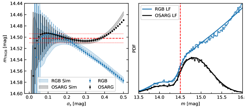
Figure 4: Simulated LFs probe the dependence of $m_{\mathrm{OSARG,mode}}$ on LF shape. Left: observed (errorbars) and simulated (shaded regions) values of $m_{\mathrm{TRGB}}$ against smoothing parameter. The simulations reproduce observed trends at a level of approximately $0.005$ mag. The simulated true $m_{\mathrm{TRGB,0}}=14.495$ coincides with the $1\sigma$ interval of our measured TRGB shown as red horizontal lines. Right: Observed (steps) and simulated (smooth curves) LFs.

Figure 5 illustrates how LF shape parameters contrast and sharpness can bias results by showing $\hat{m}=m_{\mathrm{TRGB}}-m_{\mathrm{TRGB},0}$ against $C_{-}^{+}$ and $w$ for $\sigma_{s}$$=0.15$ mag. Additionally, the right hand side illustrates graphically how these parameters change the composite LF. We find smaller bias $\hat{m}$ for higher $C_{-}^{+}$ values, qualitatively similar to Fig. 9 in Wu2022 , whose definition of contrast differs from ours. We further find that TRGB steepness, which increases with $1/w$, can lead to $\hat{m}$ at the level of $0.010$ mag, and that a steeper TRGB reduces TRGB uncertainties. Thanks to better contrast and steepness, our simulations yield smaller dispersion for OSARGs LFs. At $\sigma_{s}$$=0.15$ mag, and using the baseline parameters from Tab. 3, we find a slightly larger bias for RGBs ($\sim 0.015$ mag) than for OSARGs ($\sim 0.010$ mag). For the $\sigma_{s}$ ranges that define the results in Tab. 1, we find $\hat{m}=0.013\pm 0.009$ mag for the OSARGs simulation and $\hat{m}=0.009\pm 0.009$ mag for the RGBs simulation at $C_{-}^{+}$$=5$.

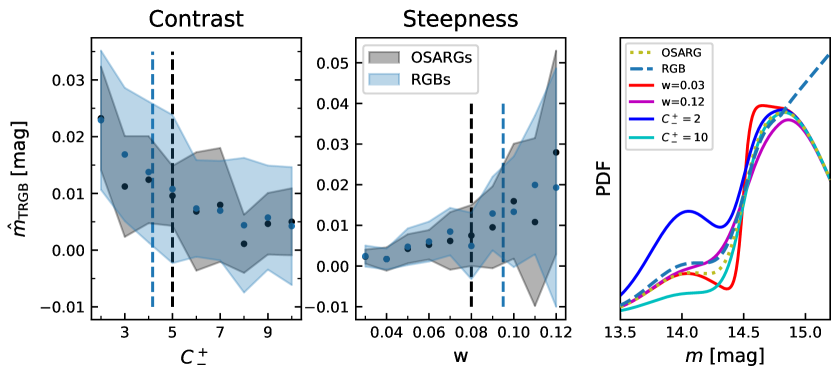
Figure 5: Investigating bias due to TRGB contrast (left) and steepness (center) for RGBs (blue) and OSARGs (black) samples at $\sigma_{s}$$=0.15$ mag. Higher contrast (larger $C_{-}^{+}$) and steeper (smaller $w$) TRGB features reduce bias and enhance precision. Vertical dashed lines indicate the values of the observed samples at $C_{-}^{+}$$=1/a_{\mathrm{AGB}}$ from Tab. 3. The right-hand panel illustrates how varying these parameter changes the OSARGs LF.

A.5 Geometric corrections

Stars belonging to different stellar populations are differently distributed in the LMC, with young stars, such as classical Cepheids being located more centrally and in a disk-like structure, whereas the old population traced by RR Lyrae stars is distributed in a somewhat asymmetric, more spherical, halo structure (e.g. OGLEing16Cephs, ; OGLEing17RRL, ). Evidence of tidal deformations and a population-dependent “bridge” linking LMC and SMC complete the picture (OGLEing2020Cephs, ; OGLEing20RRL, ; Cusano_21, ; SaroonLMCwarp22, ; Gatto2022, ). For Cepheids, geometric corrections are commonly applied to mitigate LL scatter introduced by the inclination of the young stellar population along the line of sight (e.g. Breuval2022, ). For RGB stars belonging to the old population, it is less clear whether the same geometric corrections should be applied.

We tested whether geometric corrections from the literature reduce PL sequence scatter compared to the uncorrected Bseq sample. This constitutes a strong test of the applicability of geometric corrections to the LMC’s RGB star population that does not directly affect the TRGB measurement and is independent of extinction residuals. To this end, we isolated the stars belonging to the B-sequence using a $3\sigma$ interval around the period-Wesenheit relation using the Wesenheit formulation $W_{I}=I-1.457\cdot(V-I)$, whose coefficient was calculated using the same procedure as in Sect. A.6. We found that quadratic relations best represent both sequences, and we obtain $W_{I}=12.434-4.582\cdot\log(P_{1}/20\mathrm{d})-2.098\cdot(\log(P_{1}/20\mathrm{d}))^{2}$ for the A-sequence, and $W_{I}=12.290-5.096\cdot\log(P_{1}/35\mathrm{d})-2.414\cdot(\log(P_{1}/35\mathrm{d}))^{2}$ for the B-sequence, with $\log$ of base 10. The adopted pivot periods are close to the sample medians. PL scatter was then simply computed as the rms scatter of the PL residuals.

Our test revealed no improvement in residual scatter, which is $0.148$ mag and $0.202$ mag for both sequences before geometric corrections. PL dispersion increases when applying any of the geometric corrections from the literature, specifically to (Aseq/Bseq) $0.153/0.207$ mag (Pietrzynski19, ), $0.156/0.209$ mag (Cusano_21, ), and $0.158/0.211$ mag (Hoyt2021, ). Repeating the same analysis using subsamples of OSARGs (depending whether the shortest or second shortest period falls on the B-sequence) or larger regions around the LL ($5\sigma$, $10\sigma$) consistently reveals the lowest scatter when no geometric corrections are applied. We further measured $C_{-}^{+}$ before and after applying the same geometric corrections and found no significant changes. In conclusion, we found no evidence for a need to apply geometric corrections to our samples of LMC red giants.

A.6 Reddening and extinction corrections

We use color excesses, $E(V-I)$, based on LMC Red Clump standard crayons (Skowron2021ApJS, ) to de-redden observations using $(V-I)_{0}=(V-I)-E(V-I)$. We add a systematic uncertainty of $0.014$ mag in quadrature to individual photometric uncertainties during dereddening to account for the RMS scatter of Red Clump-based color excesses, cf. (Skowron2021ApJS, ). Total extinction is corrected as $I_{0}=I-A_{I}$ with $A_{I}=R_{I}\cdot E(V-I)$. $R_{I}=1.460$ was calculated using pysynphot (pysynphot, ) for an $R_{V}=3.3$ Fitzpatrick (Fitzpatrick1999, ) reddening law recalibrated by Schlafly & Finkbeiner (Schlafly2011, ) and a star near the TRGB (Anderson2022, ). For the other bands used here, we find $R_{\mathrm{ACS,F814W}}=1.408$, $R_{G_{Rp}}=1.486$, and $R_{\mathrm{Gaia,G}}=1.852$. Systematic uncertainties related to $R_{I}$ are mitigated by limiting the analysis to stars with low color excess, $E(V-I)\leq 0.2$, so that a $10\%$ error on $R_{I}$ results in a maximum difference of $0.02$ mag.

References

- \bibcommenthead
- (1) Planck Collaboration et al. Planck 2018 results. VI. Cosmological parameters. A&A 641, A6 (2020). 10.1051/0004-6361/201833910, arXiv:1807.06209 [astro-ph.CO].
- (2) Riess, A. G. et al. A Comprehensive Measurement of the Local Value of the Hubble Constant with 1 km s-1 Mpc-1 Uncertainty from the Hubble Space Telescope and the SH0ES Team. ApJ 934 (1), L7 (2022). 10.3847/2041-8213/ac5c5b, arXiv:2112.04510 [astro-ph.CO].
- (3) Di Valentino, E. et al. In the realm of the Hubble tension-a review of solutions. Classical and Quantum Gravity 38 (15), 153001 (2021). 10.1088/1361-6382/ac086d, arXiv:2103.01183 [astro-ph.CO].
- (4) Freedman, W. L. Measurements of the Hubble Constant: Tensions in Perspective. ApJ 919 (1), 16 (2021). 10.3847/1538-4357/ac0e95, arXiv:2106.15656 [astro-ph.CO].
- (5) Lemaître, G. Un Univers homogène de masse constante et de rayon croissant rendant compte de la vitesse radiale des nébuleuses extra-galactiques. Annales de la Société Scientifique de Bruxelles 47, 49–59 (1927) .
- (6) Hubble, E. A Relation between Distance and Radial Velocity among Extra-Galactic Nebulae. Proceedings of the National Academy of Science 15 (3), 168–173 (1929). 10.1073/pnas.15.3.168 .
- (7) Lindegren, L. et al. Gaia Early Data Release 3. The astrometric solution. A&A 649, A2 (2021). 10.1051/0004-6361/202039709, arXiv:2012.03380 [astro-ph.IM].
- (8) Pietrzyński, G. et al. A distance to the large magellanic cloud that is precise to one per cent. Nature 567 (7747), 200–203 (2019). URL https://doi.org/10.1038%2Fs41586-019-0999-4. 10.1038/s41586-019-0999-4 .
- (9) Reid, M. J., Pesce, D. W. & Riess, A. G. An Improved Distance to NGC 4258 and Its Implications for the Hubble Constant. ApJ 886 (2), L27 (2019). 10.3847/2041-8213/ab552d, arXiv:1908.05625 [astro-ph.GA].
- (10) Riess, A. G. et al. Cluster Cepheids with High Precision Gaia Parallaxes, Low Zero-point Uncertainties, and Hubble Space Telescope Photometry. ApJ 938 (1), 36 (2022). 10.3847/1538-4357/ac8f24, arXiv:2208.01045 [astro-ph.CO].
- (11) Freedman, W. L. et al. The Carnegie-Chicago Hubble Program. VIII. An Independent Determination of the Hubble Constant Based on the Tip of the Red Giant Branch. ApJ 882 (1), 34 (2019). 10.3847/1538-4357/ab2f73, arXiv:1907.05922 [astro-ph.CO].
- (12) Rizzi, L. et al. Tip of the Red Giant Branch Distances. II. Zero-Point Calibration. ApJ 661 (2), 815–829 (2007). 10.1086/516566, arXiv:astro-ph/0701518 [astro-ph].
- (13) Soltis, J., Casertano, S. & Riess, A. G. The Parallax of Centauri Measured from Gaia EDR3 and a Direct, Geometric Calibration of the Tip of the Red Giant Branch and the Hubble Constant. ApJ 908 (1), L5 (2021). 10.3847/2041-8213/abdbad, arXiv:2012.09196 [astro-ph.GA].
- (14) Anand, G. S., Tully, R. B., Rizzi, L., Riess, A. G. & Yuan, W. Comparing Tip of the Red Giant Branch Distance Scales: An Independent Reduction of the Carnegie-Chicago Hubble Program and the Value of the Hubble Constant. ApJ 932 (1), 15 (2022). 10.3847/1538-4357/ac68df, arXiv:2108.00007 [astro-ph.CO].
- (15) Hoyt, T. J. On Zero Point Calibration of the Red Giant Branch Tip in the Magellanic Clouds. arXiv e-prints arXiv:2106.13337 (2021). 10.48550/arXiv.2106.13337, arXiv:2106.13337 [astro-ph.GA].
- (16) Renzini, A., Greggio, L., Ritossa, C. & Ferrario, L. Why Stars Inflate to and Deflate from Red Giant Dimensions. ApJ 400, 280 (1992). 10.1086/171995 .
- (17) Salaris, M. & Girardi, L. Tip of the Red Giant Branch distances to galaxies with composite stellar populations. MNRAS 357 (2), 669–678 (2005). 10.1111/j.1365-2966.2005.08689.x, arXiv:astro-ph/0412156 [astro-ph].
- (18) Lee, M. G., Freedman, W. L. & Madore, B. F. The Tip of the Red Giant Branch as a Distance Indicator for Resolved Galaxies. ApJ 417, 553 (1993). 10.1086/173334 .
- (19) Sakai, S., Madore, B. F. & Freedman, W. L. Tip of the Red Giant Branch Distances to Galaxies. III. The Dwarf Galaxy Sextans A. ApJ 461, 713 (1996). 10.1086/177096 .
- (20) Méndez, B. et al. Deviations from the Local Hubble Flow. I. The Tip of the Red Giant Branch as a Distance Indicator. AJ 124 (1), 213–233 (2002). 10.1086/341168, arXiv:astro-ph/0204192 [astro-ph].
- (21) Madore, B. F. et al. The Near-infrared Tip of the Red Giant Branch. I. A Calibration in the Isolated Dwarf Galaxy IC 1613. ApJ 858 (1), 11 (2018). 10.3847/1538-4357/aab7f4, arXiv:1803.01278 [astro-ph.GA].
- (22) Hatt, D. et al. The carnegie-chicago hubble program. II. the distance to IC 1613: The tip of the red giant branch and RR lyrae period–luminosity relations. The Astrophysical Journal 845 (2), 146 (2017). URL https://doi.org/10.3847%2F1538-4357%2Faa7f73. 10.3847/1538-4357/aa7f73 .
- (23) Udalski, A. et al. The Optical Gravitational Lensing Experiment. OGLE-III Photometric Maps of the Large Magellanic Cloud. Acta Astron. 58, 89–102 (2008). 10.48550/arXiv.0807.3889, arXiv:0807.3889 [astro-ph].
- (24) Stebbins, J. & Huffer, C. M. The constancy of the light of red stars. Publications of the Washburn Observatory 15, 140–174 (1930) .
- (25) Wood, P. R. et al. Le Bertre, T., Lebre, A. & Waelkens, C. (eds) MACHO observations of LMC red giants: Mira and semi-regular pulsators, and contact and semi-detached binaries. (eds Le Bertre, T., Lebre, A. & Waelkens, C.) Asymptotic Giant Branch Stars, Vol. 191, 151 (1999).
- (26) Wray, J. J., Eyer, L. & Paczyński, B. OGLE small-amplitude variables in the Galactic bar. MNRAS 349 (3), 1059–1068 (2004). 10.1111/j.1365-2966.2004.07587.x, arXiv:astro-ph/0310578 [astro-ph].
- (27) Eyer, L. Search for QSO Candidates in OGLE-II Data. Acta Astron. 52, 241–262 (2002). 10.48550/arXiv.astro-ph/0206074, arXiv:astro-ph/0206074 [astro-ph].
- (28) Kiss, L. L. & Bedding, T. R. Red variables in the OGLE-II data base - I. Pulsations and period-luminosity relations below the tip of the red giant branch of the Large Magellanic Cloud. MNRAS 343 (3), L79–L83 (2003). 10.1046/j.1365-8711.2003.06931.x, arXiv:astro-ph/0306426 [astro-ph].
- (29) Soszyński, I. et al. The Optical Gravitational Lensing Experiment. Small Amplitude Variable Red Giants in the Magellanic Clouds. Acta Astron. 54, 129–152 (2004). 10.48550/arXiv.astro-ph/0407057, arXiv:astro-ph/0407057 [astro-ph].
- (30) Soszyński, I. et al. The optical gravitational lensing experiment. the ogle-iii catalog of variable stars. iv. long-period variables in the large magellanic cloud. Acta Astronomica (2009). URL https://arxiv.org/abs/0910.1354. 10.48550/ARXIV.0910.1354 .
- (31) Kiss, L. L. & Bedding, T. R. Red variables in the OGLE-II data base - II. Comparison of the Large and Small Magellanic Clouds. MNRAS 347 (4), L83–L87 (2004). 10.1111/j.1365-2966.2004.07519.x, arXiv:astro-ph/0312237 [astro-ph].
- (32) Takayama, M., Saio, H. & Ita, Y. On the pulsation modes of OGLE small amplitude red giant variables in the LMC. Monthly Notices of the Royal Astronomical Society 431 (4), 3189–3195 (2013). URL https://doi.org/10.1093%2Fmnras%2Fstt398. 10.1093/mnras/stt398 .
- (33) Wood, P. R. The pulsation modes, masses and evolution of luminous red giants. MNRAS 448 (4), 3829–3843 (2015). 10.1093/mnras/stv289, arXiv:1502.03137 [astro-ph.SR].
- (34) Trabucchi, M. et al. Modelling long-period variables - II. Fundamental mode pulsation in the non-linear regime. MNRAS 500 (2), 1575–1591 (2021). 10.1093/mnras/staa3356, arXiv:2010.13654 [astro-ph.SR].
- (35) Riello, M. et al. Gaia Early Data Release 3. Photometric content and validation. A&A 649, A3 (2021). 10.1051/0004-6361/202039587, arXiv:2012.01916 [astro-ph.IM].
- (36) Gaia Collaboration et al. Gaia Data Release 3: The Galaxy in your preferred colours. Synthetic photometry from Gaia low-resolution spectra. arXiv e-prints arXiv:2206.06215 (2022). 10.48550/arXiv.2206.06215, arXiv:2206.06215 [astro-ph.SR].
- (37) Skowron, D. M. et al. OGLE-ing the Magellanic System: Optical Reddening Maps of the Large and Small Magellanic Clouds from Red Clump Stars. ApJS 252 (2), 23 (2021). 10.3847/1538-4365/abcb81, arXiv:2006.02448 [astro-ph.SR].
- (38) Fitzpatrick, E. L. Correcting for the Effects of Interstellar Extinction. PASP 111 (755), 63–75 (1999). 10.1086/316293, arXiv:astro-ph/9809387 [astro-ph].
- (39) Schlafly, E. F. & Finkbeiner, D. P. Measuring Reddening with Sloan Digital Sky Survey Stellar Spectra and Recalibrating SFD. ApJ 737 (2), 103 (2011). 10.1088/0004-637X/737/2/103, arXiv:1012.4804 [astro-ph.GA].
- (40) Anderson, R. I. Relativistic corrections for measuring Hubble’s constant to 1% using stellar standard candles. A&A 658, A148 (2022). 10.1051/0004-6361/202141644, arXiv:2108.09067 [astro-ph.CO].
- (41) Wu, J. et al. Comparative Analysis of TRGBs (CATs) from Unsupervised, Multi-Halo-Field Measurements: Contrast is Key. arXiv e-prints arXiv:2211.06354 (2022). 10.48550/arXiv.2211.06354, arXiv:2211.06354 [astro-ph.CO].
- (42) Cioni, M. R. L., van der Marel, R. P., Loup, C. & Habing, H. J. The tip of the red giant branch and distance of the Magellanic Clouds: results from the DENIS survey. A&A 359, 601–614 (2000). 10.48550/arXiv.astro-ph/0003223, arXiv:astro-ph/0003223 [astro-ph].
- (43) Krisciunas, K. et al. The Carnegie Supernova Project. I. Third Photometry Data Release of Low-redshift Type Ia Supernovae and Other White Dwarf Explosions. AJ 154 (5), 211 (2017). 10.3847/1538-3881/aa8df0, arXiv:1709.05146 [astro-ph.IM].
- (44) Jang, I. S. & Lee, M. G. The Tip of the Red Giant Branch Distances to Type Ia Supernova Host Galaxies. IV. Color Dependence and Zero-point Calibration. ApJ 835 (1), 28 (2017). 10.3847/1538-4357/835/1/28, arXiv:1611.05040 [astro-ph.GA].
- (45) Hoyt, T. J. et al. The Carnegie Chicago Hubble Program X: Tip of the Red Giant Branch Distances to NGC 5643 and NGC 1404. ApJ 915 (1), 34 (2021). 10.3847/1538-4357/abfe5a, arXiv:2101.12232 [astro-ph.GA].
- (46) Cerny, W. et al. Multi-Wavelength, Optical (VI) and Near-Infrared (JHK) Calibration of the Tip of the Red Giant Branch Method based on Milky Way Globular Clusters. arXiv e-prints arXiv:2012.09701 (2020). 10.48550/arXiv.2012.09701, arXiv:2012.09701 [astro-ph.GA].
- (47) Brout, D. et al. The Pantheon+ Analysis: Cosmological Constraints. ApJ 938 (2), 110 (2022). 10.3847/1538-4357/ac8e04, arXiv:2202.04077 [astro-ph.CO].
- (48) Scolnic, D. et al. The Pantheon+ Analysis: The Full Data Set and Light-curve Release. ApJ 938 (2), 113 (2022). 10.3847/1538-4357/ac8b7a, arXiv:2112.03863 [astro-ph.CO].
- (49) Yuan, W. et al. Absolute Calibration of Cepheid Period-Luminosity Relations in NGC 4258. ApJ 940 (1), 64 (2022). 10.3847/1538-4357/ac51db, arXiv:2203.06681 [astro-ph.GA].
- (50) Gaia Collaboration et al. The Gaia mission. A&A 595, A1 (2016). 10.1051/0004-6361/201629272, arXiv:1609.04153 [astro-ph.IM].
- (51) Luri, X. et al. Gaia early data release 3. Astronomy & Astrophysics 649, A7 (2021). URL https://doi.org/10.1051%2F0004-6361%2F202039588. 10.1051/0004-6361/202039588 .
- (52) Nardiello, D. et al. The Hubble Space Telescope UV Legacy Survey of Galactic Globular Clusters - XVII. Public Catalogue Release. MNRAS 481 (3), 3382–3393 (2018). 10.1093/mnras/sty2515, arXiv:1809.04300 [astro-ph.SR].
- (53) Gaia Collaboration et al. Gaia Early Data Release 3. Structure and properties of the Magellanic Clouds. A&A 649, A7 (2021). 10.1051/0004-6361/202039588, arXiv:2012.01771 [astro-ph.GA].
- (54) Wood, P. R. Variable Red Giants in the LMC: Pulsating Stars and Binaries? PASA 17 (1), 18–21 (2000). 10.1071/AS00018 .
- (55) Bono, G., Castellani, V. & Marconi, M. Classical Cepheid Pulsation Models. III. The Predictable Scenario. ApJ 529 (1), 293–317 (2000). 10.1086/308263, arXiv:astro-ph/9908014 [astro-ph].
- (56) Anderson, R. I., Saio, H., Ekström, S., Georgy, C. & Meynet, G. On the effect of rotation on populations of classical Cepheids. II. Pulsation analysis for metallicities 0.014, 0.006, and 0.002. A&A 591, A8 (2016). 10.1051/0004-6361/201528031, arXiv:1604.05691 [astro-ph.SR].
- (57) Lah, P., Kiss, L. L. & Bedding, T. R. Red variables in the OGLE-II data base - III. Constraints on the three-dimensional structures of the Large and Small Magellanic Clouds. MNRAS 359 (1), L42–L46 (2005). 10.1111/j.1745-3933.2005.00033.x, arXiv:astro-ph/0502440 [astro-ph].
- (58) Persson, S. E. et al. New cepheid period-luminosity relations for the large magellanic cloud: 92 near-infrared light curves. The Astronomical Journal 128 (5), 2239–2264 (2004). URL https://doi.org/10.1086/424934. 10.1086/424934 .
- (59) Harris, C. R. et al. Array programming with NumPy. Nature 585 (7825), 357–362 (2020). URL https://doi.org/10.1038/s41586-020-2649-2. 10.1038/s41586-020-2649-2 .
- (60) Jacyszyn-Dobrzeniecka, A. M. et al. OGLE-ing the Magellanic System: Three-Dimensional Structure of the Clouds and the Bridge Using Classical Cepheids. Acta Astron. 66 (2), 149–196 (2016). 10.48550/arXiv.1602.09141, arXiv:1602.09141 [astro-ph.GA].
- (61) Jacyszyn-Dobrzeniecka, A. M. et al. OGLE-ing the Magellanic System: Three-Dimensional Structure of the Clouds and the Bridge using RR Lyrae Stars. Acta Astron. 67 (1), 1–35 (2017). 10.32023/0001-5237/67.1.1, arXiv:1611.02709 [astro-ph.GA].
- (62) Jacyszyn-Dobrzeniecka, A. M. et al. OGLE-ing the Magellanic System: Cepheids in the Bridge. ApJ 889 (1), 25 (2020). 10.3847/1538-4357/ab61f1, arXiv:1904.08220 [astro-ph.SR].
- (63) Jacyszyn-Dobrzeniecka, A. M. et al. OGLE-ing the Magellanic System: RR Lyrae Stars in the Bridge. ApJ 889 (1), 26 (2020). 10.3847/1538-4357/ab61f2, arXiv:1904.07888 [astro-ph.SR].
- (64) Cusano, F. et al. The VMC survey – XLII. near-infrared period–luminosity relations for RR lyrae stars and the structure of the large magellanic cloud. Monthly Notices of the Royal Astronomical Society 504 (1), 1–15 (2021). URL https://doi.org/10.1093%2Fmnras%2Fstab901. 10.1093/mnras/stab901 .
- (65) Saroon, S. & Subramanian, S. Shape of the outer stellar warp in the Large Magellanic Cloud disk. arXiv e-prints arXiv:2207.13269 (2022). arXiv:2207.13269 [astro-ph.GA].
- (66) Gatto, M. et al. Discovery of NES, an Extended Tidal Structure in the Northeast of the Large Magellanic Cloud. ApJ 931 (1), 19 (2022). 10.3847/1538-4357/ac602c, arXiv:2203.13298 [astro-ph.GA].
- (67) Breuval, L., Riess, A. G., Kervella, P., Anderson, R. I. & Romaniello, M. An Improved Calibration of the Wavelength Dependence of Metallicity on the Cepheid Leavitt Law. ApJ 939 (2), 89 (2022). 10.3847/1538-4357/ac97e2, arXiv:2205.06280 [astro-ph.GA].
- (68) STScI Development Team. pysynphot: Synthetic photometry software package. Astrophysics Source Code Library, record ascl:1303.023 (2013). 1303.023.