Abstract

In-memory computing with resistive crossbar arrays has been suggested to accelerate deep-learning workloads in highly efficient manner. To unleash the full potential of in-memory computing, it is desirable to accelerate the training as well as inference for large deep neural networks. In the past, specialized in-memory training algorithms have been proposed that not only accelerate the forward and backward passes, but also establish tricks to update the weight in-memory and in parallel. However, the state-of-the-art algorithm ( Tiki-Taka version 2 (TTv2)) still requires near perfect offset correction and suffers from potential biases that might occur due to programming and estimation inaccuracies, as well as longer-term instabilities of the device materials. Here we propose and describe two new and improved algorithms for in-memory computing ( Chopped-TTv2 (c-TTv2) and Analog Gradient Accumulation with Dynamic reference (AGAD)), that retain the same runtime complexity but correct for any remaining offsets using choppers. These algorithms greatly relax the device requirements and thus expanding the scope of possible materials potentially employed for such fast in-memory DNN training.

1 Introduction

In-memory computing with resistive crossbar arrays could greatly accelerate deep-learning workloads, since energy efficient acceleration can be achieved by implementing ubiquitous matrix-vector multiplications using resistive elements and fundamental physics (Kirchhoff’s and Ohm’s laws) Sebastian et al. (2020); Burr et al. (2017); Haensch et al. (2019); Yang et al. (2013); Sze et al. (2017). While most prototype chip building efforts to-date have been focused on accelerating the inference phase of pre-trained DNNs Wan et al. (2022); Khaddam-Aljameh et al. (2021); Xue et al. (2021); Fick et al. (2022); Narayanan et al. (2021); Ambrogio et al. (2018); Yao et al. (2020), in terms of raw compute requirements, the training phase typically is orders of magnitude more expensive than inference, and thus would in principle have a greater need for hardware acceleration using in-memory compute Gokmen & Vlasov (2016). However, in-memory training using non-volatile memory elements has been challenging, in particular because of the asymmetric and non-ideal switching of the memory devices, and the much greater precision requirements during gradient update (see e.g. Jain et al. (2019) for a discussion).

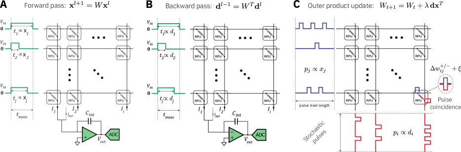
Figure 1: Physical implementaton of in-memory matrix-vector multiplication (MVM) for forward and backward passes and outer product update according to Gokmen & Vlasov (2016).

To accelerate the stochastic gradient descent (SGD) of DNN training, not only the forward pass, but also the backward pass, as well as gradient computation and update needs to be considered. While the backward pass of a linear layer is straightforwardly accelerated in-memory by transposing the inputs and outputs, the gradient accumulation and update is more difficult to perform in a fast and efficient manner in-memory. One way is to sacrifice speed and efficiency by computing the gradient and its accumulation in digital and only accelerating the forward and backward pass in-memory, as suggested by Nandakumar et al. (2018; 2020). On the other hand, Gokmen et al. Gokmen & Vlasov (2016) suggested to use the coincidence of stochastic pulses to efficiently perform the outer product update operation fully in-memory in a highly efficient and parallel manner. However, in its initial naive formulation, a bi-directionally switching device of high symmetry and precision (in terms of reliability of incremental conductance changes) is needed to be able to compute and accumulate the gradients with the required accuracy Agarwal et al. (2016); Gokmen & Vlasov (2016). Further refinements of the algorithm, however, relaxed the requirements of the number of reliable conductance state and the device symmetry considerably Gokmen & Haensch (2020); Gokmen (2021).

In the latest installment, the so-called TTv2 learning algorithm Gokmen (2021), three tunable conductance elements for each weight matrix element are required, namely the matrices $\breve{A}$, $\breve{R}$, and $\breve{W}$. The first two conductances, $\breve{A}$ and $\breve{R}$, are used to perform the outer product and (parts of) the gradient accumulation, whereas $\breve{W}$ is used as the representation of the weight $W$ of a linear layer and thus used in the forward and backward passes. On functional level, the algorithm is similar to modern SGD methods that introduce a momentum term (such as ADAM Kingma & Ba (2014)), since also here the gradient is first computed and accumulated in a leaky fashion onto a separate matrix before being added to the weight matrix. However, the analog friendly TTv2 algorithm computes and transfers the accumulated gradients asynchronously for each row (or column) to gain run-time advantages. Furthermore, crucially, the device asymmetry of the memory element causes an input-dependent decay of the recent accumulated gradients as opposed to the usual constant decay rate of the momentum term that is difficult to efficiently implement in-memory (see also discussion in Gokmen (2021); Onen et al. (2022)).

In more detail, for each update, the outer product gradient update is first computed onto $\breve{A}$ using coincidences of stochastic pulse trains. Then $\breve{A}$ is read in a row-wise (or column-wise) fashion and the read-out accumulated gradients are additionally filtered onto a digital storage (hidden) matrix $H$ to smooth high frequency noise introduced by the gradient computation itself as well as the physical writing process using stochastic pulses on noisy materials. Only when a threshold of the accumulated gradient is reached, a single writing pulse is sent to the corresponding weight element of the matrix $\breve{W}$.

While this TTv2 algorithm greatly improves the material specifications by introducing low-pass filtering of the recent gradients, it hinges on the assumption that the device has a pre-defined and stable symmetry point (SP) within its conductance range Onen et al. (2022). The SP is defined as the conductance value where a positive and a negative update will result on average in the same net change of the conductance. Because of the assumed device asymmetry, the SP acts as a stable fix point for random inputs, which causes the accumulated gradient on $\breve{A}$ to automatically decay near convergence. However, to induce a decay towards zero algorithmically, it is essential to identify the SP with the zero value for each device, which is achieved by removing the offset using a reference array $\breve{R}$. The reference conductance $\breve{R}$ is thus used to store the SP values of its corresponding devices of $\breve{A}$ and when accessing $\breve{A}$, instead of directly reading $\breve{A}$, the difference $\breve{A}-\breve{R}$ is read instead, while only $\breve{A}$ is updated during training.

Programming the offset array $\breve{R}$ to the SP of $\breve{A}$ once at the beginning could be problematic in practice since any remaining offset $\breve{A}-\breve{R}+\Delta$ would be continuously read and added onto the weight matrix $\breve{W}$. Such constant offset $\Delta$ from the fixed point might arise for instance by an inaccurate estimation or writing of the SP onto $\breve{R}$ or a long-term temporal variation the SP of $\breve{A}$. Moreover, offset transients caused by temporally $\breve{A}\neq\breve{R}$ might result in significant gradient accumulation and writing onto $\breve{W}$, thus possibly leading to oscillations and non-optimal learning behavior.

In this paper, we propose two new algorithms based on TTv2, that improve the gradient computation in case of any kinds of reference instability or residual offsets. Both algorithms introduce a technique borrowed from amplifier circuit design, called chopper Enz & Temes (1996). A chopper is a well-known technique to remove any offsets or residuals caused by the accumulating system that are not present in the signal, by modulating the signal with a random sign-change (the chopper) that is then corrected for when reading from the accumulator. In our first algorithm, we randomly flip the sign of the activation or error vector before computing the outer product update in-memory. After reading $\breve{A}-\breve{R}$, the read value is then again sign-corrected. In this way, any remaining offset residuals are averaged out by the filtering stage without significantly increasing the complexity of the algorithm. In the second new algorithm, we propose to additionally use an on-the-fly dynamic estimation of the recent reference point that further improves on removing transients and essentially obliterates the requirement of having a tunable reference array $\breve{R}$ altogether.

Algorithm 1 Parallel in-memory update using dynamically adjusted stochastic pulsing.

0:  data vector $x_{i}$, size $n$, gradient vector $d_{j}$, size $m$, weight matrix $\breve{w}_{ij}$, average pulse size at SP $\delta_{w}$, learning rate $\eta$, max pulses $l_{\text{max}}$

0:  Updated analog weight matrix $\breve{w}_{ij}$

  set $m_{x}\leftarrow\max_{i}|x_{i}|$ and $m_{d}\leftarrow\max_{j}|d_{j}|$

  set $\kappa\leftarrow\frac{\eta m_{x}m_{d}}{\delta_{w}}$

  set $l\leftarrow\min(l_{\text{max}},\left\lceil\kappa\right\rceil)$ and $\tilde{m}_{d}\leftarrow m_{d}\min(\frac{l_{\text{max}}}{\kappa},1)$

  set $a\leftarrow\sqrt{\frac{\eta\,m_{x}}{l\,\tilde{m}_{d}\delta_{w}}}$ and $b\leftarrow\sqrt{\frac{\eta\,\tilde{m}_{d}}{l_{\text{max}}\,m_{x}\delta_{w}}}$

  for $k=1$ to $l$ do

     set all $q_{i}\leftarrow 0$ and all $p_{j}\leftarrow 0$

     for $i=1$ to $m$ do

        Draw random number $\xi\in{\cal U}(0,1)$

        if $a|d_{i}|<\xi$ then

           set $q_{i}\leftarrow\operatorname{sgn}(d_{i})$

        end if

     end for

     for $j=1$ to $n$ do

        Draw random number $\xi\in{\cal U}(0,1)$

        if $b|x_{j}|<\xi$ then

           set $p_{j}\leftarrow\operatorname{sgn}(x_{j})$

        end if

     end for

     {Send pulse vectors $\mathbf{p}$ and $\mathbf{q}$ to update $\breve{w}_{ij}$:}

     for $i=1$ to $m$ do

        for $j=1$ to $n$ do

           if $p_{j}\neq 0$ and $q_{i}\neq 0$ then

              set $\breve{w}_{ij}\leftarrow\breve{w}_{ij}+dF\left(\breve{w}_{ij}|\boldsymbol{\theta},\,{}\operatorname{sgn}(q_{i}p_{j})\right)$

           end if

        end for

     end for

  end for

2 Background: In-memory optimizer

2.1 Analog matrix-vector multiplication

Using resistive crossbar arrays to compute an MVM in-memory has been suggested early on Steinbuch (1961), and multiple prototype chips where MVMs of DNNs during inference are accelerated have been described Wan et al. (2022); Khaddam-Aljameh et al. (2021); Xue et al. (2021); Fick et al. (2022); Narayanan et al. (2021). In principle, in all these solutions, the weights of a linear layer are stored in a crossbar array of tunable conductances, inputs are encoded e.g. in voltage pulses and Ohm’s and Kirchhoff’s law are used to multiply the weights with the inputs and accumulate the products, respectively (Fig. 1A, see also e.g. Sebastian et al. (2020) for more details). In many designs, the resulting currents or charge, is converted back to digital by highly parallel analog-to-digital converters.

For fully in-memory analog training, as suggested in Gokmen & Vlasov (2016), additionally a transposed MVM has to be implemented for the backward pass, which can be achieved by transposing input and output accordingly (see Fig. 1B).

2.2 In-memory outer product update

While accelerating the forward and the backward pass of SGD using in-memory MVMs is promising, for a full in-memory training solution, in-memory gradient computation and weight update have to be considered for acceleration as well: it is the remaining operation having ${\cal O}(n^{2})$ complexity (where $n\times n$ is the size of the matrix in “analog”) during DNN training Gokmen & Vlasov (2016).

For the gradient accumulation of a weight matrix $W$ of a linear layer (i.e. computing $\mathbf{y}=W\mathbf{x}$), the outer product update of $W\leftarrow W+\lambda\mathbf{d}\mathbf{x}^{T}$ needs to be computed. While this can be done in digital, possibly exploiting sparseness (e.g. see Nandakumar et al. (2020)), it would still require ${\cal O}(n^{2})$ digital operations, and doing so would thus limit the overall acceleration factor obtainable for in-memory training. To accelerate also the outer-product update to be performed in-memory and fully parallel, Gokmen et al. Gokmen & Vlasov (2016) suggested to use stochastic pulse trains and their coincidence (as illustrated in Fig. 1 C).

The exact update algorithm has gone through a number of improvements in recent years Gokmen et al. (2017; 2018), however, we here suggest to use a yet improved version in Alg. 1. In particular, the pulse trains are dynamically adjusted in length in our version. Note that we here assume for simplicity that negative pulses can be sent. In practice negative and positive pulses are sent in sequential phases.

While Gokmen & Vlasov (2016); Gokmen et al. (2017; 2018) have investigated the noise properties when using Alg. 1 to directly implement the gradient update in-memory, it turns out that this would require very symmetric switching characteristics of the memory device elements. Thus, the requirements of such a “in-memory plain SGD” algorithm turns out to be challenging in particular in face of the asymmetry observed in today’s materials, which we discuss in the next section.

2.3 Device material model

When subject to a large enough voltage pulse, bi-directionally switching device materials, such as resistive random access memories (ReRAM) Zahoor et al. (2020), typically show a high degree of asymmetry in one versus the other direction and gradual saturation to a minimal maximal conductance value. In previous studies Fusi & Abbott (2007); Frascaroli et al. (2018), it was shown that the “soft-bounds” model characterizes the switching behaviour qualitatively well. According to that model, the weight change $w\leftarrow w+dF\left(w|\boldsymbol{\theta},\,{}D\right)$ to a single update pulse in either up ($D=+$ or down $D=-$) direction is given by

$$dF\left(w|\boldsymbol{\theta},\,{}+\right) = \alpha_{+}\frac{b_{\text{max}}-w}{b_{\text{max}}}(1+\sigma_{\text{c-to-c}}\xi)$$ (1)

$$dF\left(w|\boldsymbol{\theta},\,{}-\right) = {}-\alpha_{-}\frac{b_{\text{min}}-w}{b_{\text{min}}}(1+\sigma_{\text{c-to-c}}\xi)$$

Here we use the placeholder $\boldsymbol{\theta}$ for the hyper-parameters. To capture device-to-device variability, we initially draw $b_{\text{max}}=\max(1+\sigma_{b}\xi_{1},0)$ and $b_{\text{min}}=\min(-1+\sigma_{b}\xi_{2},0)$ where the $\xi_{i}\in{\cal N}(0,1)$ are random numbers that are different for each device. The slope parameters are given by

$$\alpha_{+} = \delta_{w}\,\left(\gamma+\rho\right)$$ (2)

$$\alpha_{-} = \delta_{w}\,\left(\gamma-\rho\right)$$

where $\gamma=e^{\sigma_{\text{d-to-d}}\xi_{3}}$, and $\rho=\sigma_{\pm}\xi_{4}$, so that $\sigma_{\text{d-to-d}}$ is a hyper-parameter for the variation of the slope across devices, and $\sigma_{\pm}$ a separate device-to-device variation in the difference of the slope between up and down direction. The material parameter $\delta_{w}$ determines the average update response for one pulse when the weight is at zero. We define the number of device states by the average weight range divided by $\delta_{w}$, ie. $n_{\text{states}}=\frac{2}{\delta_{w}}$.

2.3.1 Symmetry point

It can easily be seen that for the device model Eq. 1, the update size linearly decreases for positive updates up the bound $b_{\text{max}}$, and likewise linearly decreases for negative updates down to the bound $b_{\text{min}}$, and thus the weight will saturate at $b_{\text{min}}$ and $b_{\text{max}}$. Thus there exists a weight value at which the up and down updates sizes are equal on average, which is thus called the symmetry point (SP) Gokmen & Haensch (2020); Onen et al. (2022).

Solving Eq. 1 for the SP $\breve{w}^{*}$ by requiring up and down pulse sizes to be equal, one finds

$$\breve{w}^{*}=\frac{\alpha_{+}-\alpha_{-}}{\frac{\alpha_{+}}{b_{\text{max}}}-\frac{\alpha_{-}}{b_{\text{min}}}}=\frac{2\rho}{\frac{\gamma+\rho}{b_{\text{max}}}-\frac{\gamma-\rho}{b_{\text{min}}}}$$ (3)

In summary, we use a device model that is already defined in a way that the SP is at zero when $\sigma_{\pm}=0$. However, if $\sigma_{\pm}>0$ the SP is not at zero.

Transients when decaying towards the SP

If random up-down pulsing (without a bias in one direction) is applied to the devices, the device will reach its SP. In the case where a positive pulse always follows a negative pulse, the weight change (assuming for the moment $\sigma_{b}=\sigma_{\text{c-to-c}}=\sigma_{\pm}=\sigma_{\text{d-to-d}}=0$) can be written as:

$$\Delta w = dF\left(w|\boldsymbol{\theta},\,{}+\right)+dF\left(w+dF\left(w|\boldsymbol{\theta},\,{}+\right)|\boldsymbol{\theta},\,{}-\right)$$ (4)

$$\approx dF\left(w|\boldsymbol{\theta},\,{}+\right)+dF\left(w|\boldsymbol{\theta},\,{}-\right)$$

$$= \delta_{w}(1-w)-\delta_{w}(1+w)$$

$$= -2\delta_{w}w$$

which shows that for repeated pairs of up and down pulses the weight will decay exponentially with (approximate) decay rate of $\tau=2\delta_{w}$ to a fixed point at $\breve{w}^{*}=0$.

Setting the reference device to the SP

To remove the offsets arising from the decay towards the SP, some algorithms discussed below require a the reference matrix $\breve{R}$ to be set to the SP Gokmen (2021); Onen et al. (2022). We model this by setting (with Eq. 3)

$$\breve{r}_{ij}=\breve{a}^{*}_{ij}+\mu_{r}+\sigma_{r}\xi_{ij}$$ (5)

where $\xi_{ij}\in{\cal N}(0,1)$. Thus $o_{r}=\mu_{r}+\sigma_{r}\xi$ models the remaining offsets on the reference device after SP subtraction. Remaining offsets could be due to incorrectly estimating the SP of $\breve{A}$ or to the programming error when setting $\breve{R}$. The algorithm of how to program $\breve{R}$ to the SP of $\breve{A}$ in practice is discussed in Kim et al. (2019).

Algorithm 2 Chopped-TTv2 (c-TTv2) algorithm.

0:  learning rate $\lambda$, buffer scale $\gamma_{0}$, transfer period $n_{s}$, chopper probability $\rho$

0:  converged analog weights $\breve{w}_{ij}$

  set $\gamma\leftarrow\gamma_{0}\frac{\delta_{w}}{nn_{s}}$

  set counters $s$ and $k$ to 0 and digital matrix $h_{ij}\leftarrow 0$

  call Program reference $\breve{R}$ to the SP of $\breve{A}$: $\breve{r}_{ij}\leftarrow\breve{a}_{ij}^{*}$

  repeat

     call start SGD iteration for mini-batch {(using $\breve{w}_{ij}$ as weights) until the update of $\breve{w}_{ij}$ is required}

     for all inputs $\mathbf{x}$ and $\mathbf{d}$ to be updated onto $\breve{W}$ do

        call Alg. 1 to update $(c_{j}x_{j})$ and $\mathbf{d}$ onto $\breve{A}$

        set $s\leftarrow s+1$

        if $s=n_{s}$ then

           set $k\leftarrow k+1\mod n$ and $s\leftarrow 0$ and all $p_{i}\leftarrow 0$

           call the analog MVM: $\mathbf{y}\leftarrow(\breve{A}-\breve{R})\,\mathbf{e}_{k}^{(n)}$

           for $i=1$ to $m$ do

              set $h_{ik}\leftarrow h_{ik}+c_{k}\frac{\lambda}{\gamma}y_{i}$

              if $|h_{ik}|>1$ then

                 set $p_{i}\leftarrow\operatorname{sgn}(h_{ik})$

                 set $h_{ik}\leftarrow 0$

              end if

           end for

           {Use pulse vector $p_{i}$ to update column $k$ of $\breve{W}$:}

           for $i=1$ to $m$ do

              if $p_{i}\neq 0$ then

                 set $\breve{w}_{ik}\leftarrow\breve{w}_{ik}+dF\left(\breve{w}_{ik}|\boldsymbol{\theta},\,{}\operatorname{sgn}(p_{i})\right)$

              end if

           end for

           {Flip the chopper as follows.}

           draw random number $\xi\in{\cal U}(0,1)$

           if $\rho<\xi$ then

              set $c_{k}\leftarrow-c_{k}$

           end if

        end if

     end for

     call finish SGD iteration

  until convergence is reached

2.4 TTv2 algorithm

To lower the device requirements for in-memory SGD, Gokmen & Haensch (2020) proposed to first compute the outer product update in a fast manner in-memory and thus accumulate the recent past of the gradients onto a separate analog crossbar array $\breve{A}$, but slowly transfer the recent accumulated gradients by sequential vector reads (single columns or rows) of $\breve{A}$ onto the analog weight matrix $\breve{W}$, to counter-act the loss of the information due to the device asymmetry on the gradient matrix $\breve{A}$. The innovative aspect of this approach is that the accumulated gradients on $\breve{A}$ are decaying in an input dependent manner due to the device asymmetry: as discussed above, random (unbiased) input will cause the conductances on $\breve{A}$ to decay to the SPs. Thus, if the SPs are subtracted, the gradient matrix decays to zero by design when no net gradients are present as is the case at a minimum in the loss landscape.

Furthermore, since the transfer of the gradients on $\breve{A}$ to $\breve{W}$ is done with only ${\cal O}(n)$ digital operations (at most one vector per matrix update) the digital and additional computations introduced by the transfer read and write to $\breve{W}$ is not a bottleneck, as opposed to the case where the full gradient update would be done in digital that required ${\cal O}(n^{2})$ operations.

In Gokmen (2021), the algorithm was improved by additionally filtering the transferred gradient using a digital matrix $H$ that additionally accumulates the recently read gradients from $\breve{A}$ and, only once a threshold level is reached, a pulse is sent to update corresponding device of the weight matrix $\breve{W}$. This additional averaging, while introducing more digital computations, still retains the ${\cal O}(n)$ character, as at most one vector is operated on for each transfer. It was shown Gokmen (2021) that the filtering stage greatly lowers the device requirements, in particular the effective number of device states: only 15 states are enough to train an LSTM to acceptable accuracy. This relaxed device requirements now make it possible to think about current ReRAM devices for in-memory training Gong et al. (2022). This Tiki-Taka version 2 (TTv2) algorithm is our baseline comparison.

3 Improved in-memory optimizers

We here present our new algorithmic contributions as well as a new way to scale the learning rates depending on material specifications and weight matrix.

3.1 c-TTv2  algorithm

While an analog reference matrix $\breve{R}$ has the advantage to subtract the SP from $\breve{A}$ efficiently, the design choice comes with unique challenges. In particular, the programming of $\breve{R}$ might be inexact or the SP might vary on a slow time scale, introducing some remaining offset transients. However, any offsets would constantly accumulate on $H$ and be written onto in $\breve{W}$ thus biasing the weight matrix unwantedly. Moreover, the decay of $\breve{A}$ to its SP is the slower the more states the device has (see Eq. 4) and input dependent. The latter might cause the $\breve{A}$ to not decay for many updates which again would cause a bias in $\breve{W}$ (as shown below). While feedback from the loss would eventually change the gradients and correct $\breve{W}$, the learning dynamics might nevertheless be impacted.

Algorithm 3 Analog Gradient Accumulation with Dynamic reference (AGAD) algorithm.

0:  learning rate $\lambda$, buffer scale $\gamma_{0}$, transfer period $n_{s}$, chopper frequency $\rho$, leaky-average time-scale $\beta$

0:  converged analog weights $\breve{w}_{ij}$

  set $\gamma\leftarrow\gamma_{0}\frac{\delta_{w}}{nn_{s}}$

  set counters $s$, $k$ and $t$ to 0 and all choppers $c_{j}\leftarrow 1$

  set digital matrices $h_{ij}$, $\mu_{ij}$ and $\mu^{\text{past}}_{ij}$ to all 0

  repeat

     call start SGD iteration

     for all inputs $\mathbf{x}$ and $\mathbf{d}$ to be updated onto $\breve{W}$ do

        call Alg. 1 to update $c_{j}x_{j}$ and $d_{i}$ onto $\breve{a}_{ij}$

        set $s\leftarrow s+1$

        if $s=n_{s}$ then

           set $s\leftarrow 0$ and $t\leftarrow t+1$ and all $p_{i}\leftarrow 0$

           set $k\leftarrow k+1\mod n$

           call analog MVM: $\mathbf{y}\leftarrow\breve{A}\,\mathbf{e}_{k}$

           for $i=1$ to $m$ do

              set $h_{ik}\leftarrow h_{ik}+c_{k}\,\frac{\lambda}{\gamma}\left(y_{i}-\mu^{\text{past}}_{ik}\right)$

              set $\mu_{ik}\leftarrow(1-\beta)\,\mu_{ik}+\beta y_{i}$

              if $|h_{ik}|>1$ then

                 set $p_{i}\leftarrow\operatorname{sgn}(h_{ik})$

                 set $h_{ik}\leftarrow 0$

              end if

           end for

           {Use pulse vectors $p_{i}$ to update column $k$ of $\breve{W}$:}

           for $i=1$ to $m$ do

              if $p_{i}\neq 0$ then

                 $\breve{w}_{ik}\leftarrow\breve{w}_{ik}+dF\left(\breve{w}_{ik}|\boldsymbol{\theta},\,{}\operatorname{sgn}(p_{i})\right)$

              end if

           end for

           {Flip chopper and reset $\mu_{ij}$ and $\mu_{ij}^{\text{past}}$ as follows.}

           if $t\mod\left\lceil\frac{1}{\rho}\right\rceil=0$ then

              set $c_{k}\leftarrow-c_{k}$

              for $i=1$ to $m$ do

                 set $\mu_{ik}^{\text{past}}\leftarrow\mu_{ik}$

                 set $\mu_{ik}\leftarrow 0$

              end for

           end if

        end if

     end for

     call finish SGD iteration

  until convergence is reached.

To improve on any remaining bias and low-frequency noise and bias sources, we suggest here to improve the algorithm by introducing choppers. Chopper stabilization is a common method for offset correction in amplifier circuit design Enz & Temes (1996). Choppers modulate the incoming signal before gradient accumulation, and subsequently demodulate during the reading of the accumulated gradient. In more detail, we introduce choppers $c_{j}\in\{-1,1\}$ that flip the sign of each of the activations $x_{j}$ before the gradient accumulation on $\breve{A}$. When reading the $k$-th column of $\breve{A}$ to be transferred onto $H$ (as in TTv2), we apply the corresponding chopper $c_{k}$ to recover the correct sign of the signal. The choppers are then flipped randomly, see Alg. 2 for the detailed algorithm (compare also to Fig. 2).

In this manner, any low frequency component that is caused by the asymmetry or any remaining offsets and transients on $\breve{A}$ is not modulated by the chopper and thus canceled out by the sign flips. We call this algorithm Chopped-TTv2 (c-TTv2) stochastic gradient descent.

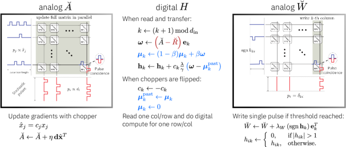
Figure 2: Improved in-memory training algorithms, c-TTv2 and AGAD. The blue color indicates equations unique and in addition for AGAD. The reference subtraction (in red) is not needed for AGAD. Removing blue equations and fixing the choppers recovers TTv2.

3.2 AGAD  algorithm

While the chopper together with the low-pass filtering greatly improve the resilience to any remaining offsets (see Sec. 4), if offsets are too large the filtering required might be too slow, thus reducing the responsiveness of the algorithm. This can be understood as follows. Assume that a constant gradient $g$ is calculated onto an single element of the gradient matrix, $\breve{a}$. Assume further two chopper phases with $k$ reads each and a reference offset $o_{r}$. Then corresponding element in the hidden matrix $h$ will receive the following changes

$$h_{t+n}-h_{t} = \lambda k\left(o_{r}+g\right)$$ (6)

$$h_{t+2n}-h_{t} = \lambda k\left(o_{r}+g-o_{r}+g\right)=2\lambda kg$$ (7)

Thus the offset is removed by the chopper sign flips and the gradient correctly recovered (Eq. 7). However, this removal becomes problematic in the step Eq. 6 if $|o_{r}|\gg|g|$ and $\lambda n|o_{r}|\approx 1$ (1 being the threshold, see Alg. 2), since the update threshold would be falsely triggered by the addition of the offset. Thus, for large offsets the learning rate $\lambda$ needs to be decreased to avoid accidentally triggering an update onto $\breve{w}$, which however slows down learning.

To improve upon this issue, we suggest an on-the-fly estimation of the reference, where we use additional digital compute to store the value of $\breve{a}$ right before the chopper sign flip and use this value as a reference instead of the reference matrix $\breve{R}$. The reasoning here is that the chopper flips are unrelated to the direction of gradient information. Thus, if a significant average gradient is currently present, the direction of updates onto $\breve{A}$ has to change its direction when the chopper flips. Thus the recent value of $\breve{a}$ can serve as good reference point to read the information on $\breve{a}$ without bias. This new algorithm is called Analog Gradient Accumulation with Dynamic reference (AGAD). See Alg. 3 and Fig. 2 for implementation details.

3.3 Learning rate scaling laws

In the original formulation of the TTv2algorithm Gokmen (2021), the learning rate $\lambda_{H}$ for writing onto the hidden matrix $H$ was not specified explicitly. We here suggest to use the scaling law

$$\lambda_{H}=\frac{\lambda\,n_{s}\,n}{\gamma_{0}\delta_{w}}$$ (8)

where $n$ is the number of columns of the weight matrix, $n_{s}$ the number of gradient updates done before a single column-read of $\breve{A}$, and $\delta_{w}$ is the average update response size at the SP of $\breve{A}$. Note that with Eq. 8 the threshold of $H$ (ie. when to write onto $\breve{W}$) effectively scales with how often a single element of the gradient matrix $\breve{A}$ was updated before a read happens and is naturally divided by a measure of the average update size $\delta_{w}$. Here $\lambda$ is the learning rate of the standard SGD, which might be scheduled. We thus do not adjust the learning rate on $\breve{A}$ but instead the writing onto $H$ by the overall SGD learning rate. The hyper-parameter $\gamma_{0}$ specifies the length of accumulation, with larger values averaging the read gradients for longer. Note, however, that the same effect is done by adjusting $\lambda$ so that tuning one of both is enough in practice.

Similarly, the learning rate $\eta$, used for the gradient update onto $\breve{A}$, is important to set correctly for the DNN at hand. Since the pulse width is finite, the gradient magnitude has to be large enough to cause a significant change on the gradient matrix $\breve{A}$, so the learning rate $\eta$ needs to be scaled accordingly. Since the gradient magnitude often differs for individual layers, and might also change over time, we dynamically divide $\eta$ by the recent running average $\mu_{x}$ and $\mu_{d}$ of the absolute maximum of the inputs $m_{x}=\max_{j}|x_{j}|$ and input gradients $m_{d}=\max_{i}|d_{i}|$, respectively.

$$\eta=\frac{\eta_{0}l_{\text{max}}\delta_{w}}{\mu_{x}\mu_{d}}$$ (9)

Note that $m_{x}$ and $m_{d}$ are needed for the gradient update already (see Alg. 1), so that this does not require any additional computations, except for the leaky average computations. Since $l_{\text{max}}\delta_{w}$ is approximately the maximum that the device material can change during one update ($l_{\text{max}}$ is the number of pulses used, see Alg. 1), the Eq. 9 means in case of $\eta_{0}=1$ that the a gradient update product $x_{i}d_{j}>\mu_{x}\mu_{d}$ is going to be clipped. The default value of $\eta_{0}$ is 1, although is some cases higher values improve learning. We use both of these scaling laws for all algorithms presented here.

4 Results

In following we present first a number of numerical test cases to illustrate and compare the mechanism of the training algorithms. Then we apply and compare them to SGD and DNN training with different material and reference offsets settings. For simulations, we used the PyTorch-based Paszke et al. (2019) open source toolkit IBM Analog Hardware Acceleration Kit (AIHWKit) Rasch et al. (2021).

4.1 Constant average gradient without offset

As an illustration of the different learning algorithm we first investigate a simple case where activations are given by $x=-X$ and gradient inputs by $d=\alpha X+(1-\alpha)Y$ where $X,Y\sim{\cal N}(0,1)$ are Gaussian random variables. Thus, in this case the correlation of activations and gradients is given by $\alpha$ and expected average update is only in one direction $\Delta\breve{w}\propto-\alpha$. The various variables are plotted against the number of updates for the three algorithms, TTv2, c-TTv2 and AGAD in Fig. 3. Here we assume that the reference matrix $\breve{R}$ is perfectly accurately set to the SP of $\breve{A}$ so that no offset remains.

Note that for TTv2 (top panel of Fig. 3) the trace of a selected $\breve{a}$ is strongly biased to negative values, thus accumulating correctly the net gradient. It, however, saturates at a certain level, caused by the characteristics of the underlying device model (see Eq. 1). Because of the occasional reads, the hidden weight accumulates until threshold is reached at $-1$ (green trace), in which case the weight $\breve{w}$ is updated by one pulse (orange trace). The shaded blue area indicates the value of $\omega=c\left(\breve{a}-\breve{r}\right)$ (where the chopper $c=1$ is not used for TTv2). The area would be red if the value was positive, which would indicate a hidden weight update in the wrong direction.

In the middle panel of Fig. 3, the behavior of the c-TTv2 algorithm is shown for the same inputs. Here, for better illustration, a fixed chopper period is chosen. Since the incoming gradient is constant (negative), the modulation with the chopper sign causes an oscillation in the accumulation of the gradient in $\breve{a}$. However, since the sign is corrected, the hidden matrix is updated (mostly) into the correct direction (blue areas are sign corrected). As we will see below, this flipping of signs will cancel out offsets (here assumed to be 0). Due to transients in this example, the trace of $\breve{a}$ has not always returned to the SP before reads, which causes some transient updates of the hidden weights in the wrong direction (red areas). The weight $\breve{w}$ is nevertheless correctly updated as the hidden weight averages out the transients successfully. The rate of change of $\breve{w}$, however, is somewhat impacted by the averaging of the transients.

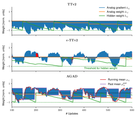
Figure 3: Mechanism of the algorithms with constant (negative) gradient input with perfect SP estimation. Parameters: $\delta_{w}=0.05$, $\sigma_{b}=\sigma_{\pm}=\sigma_{\text{d-to-d}}=\sigma_{\text{c-to-c}}=0.3$, $\gamma_{0}=200$, $\lambda=0.1$, $n_{s}=1$, $\beta=0.5$, $\rho=0.1$, $l_{\text{max}}=5$, $\eta=1$, and $\mu_{r}=\sigma_{r}=0$.

Since AGAD (Fig. 3 bottom panel) uses an (average) value $\mu^{\text{past}}$ of the recent accumulated gradient $\breve{a}$ as the reference point (and not the static SP programmed onto $\breve{R}$) it is not plagued with the same transients. In fact, the increased range causes a faster update of the hidden matrix and subsequently the weight $\breve{w}$.

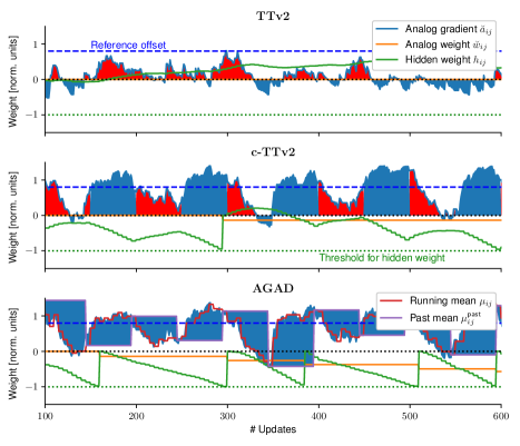
Figure 4: Mechanism of the algorithms with constant gradient input and significant reference offset. Parameters as in Fig. 3 except $\mu_{r}=0.8$.

4.2 Constant average gradient with offset

Since in Fig. 3 the reference $\breve{R}$ was set exactly to the SP, no offset from the fixed-point existed. In this case TTv2 indeed works perfectly fine and might be the algorithm of choice, because it requires least amount of digital compute. However, now we examine the situation with a large offset, so that the effective SP of $\breve{A}-\breve{R}$ is not at zero. In Fig. 4 we repeat the experiment of Fig. 3 with an offset of $\mu_{r}=0.8$ (dashed line in Fig. 4). We note that for TTv2, the constant gradient pushes the accumulated gradient $\breve{a}$ away from the SP (blue dashed line), however, since the algorithm does not take the offset into account, the update onto the hidden matrix is wrong. In fact, hidden weight $h$ (green line) is even updated in the wrong direction in this example (note that it is expected to become more negative).

On the other hand, because of the effect of the chopper, even this large bias can be successfully removed with the c-TTv2  algorithm (Fig. 4 middle panel). Note that the hidden value $h$ as well as the weight $\breve{w}$ decrease correctly. However, due to the large bias, noticeable oscillations (red areas) are stressing the accumulation on $h$, thus reducing the speed and fidelity of the gradient accumulation.

Due to the dynamic reference point computation of the AGAD algorithm, the reference offset is almost irrelevant in this case (Fig. 4 bottom panel), thus perfectly correcting for any offset.

4.3 Input-induced decay

One hallmark of the TTv2 algorithm is the input-induced decay: random input or gradient fluctuations will draw the value of $\breve{A}$ towards the SP (see Eq. 4) and thus decay to zero algorithmically (because of the reference $\breve{R}$, see Eq. 5). This is shown in Fig. A.3, where it is shown the hidden matrix decays quickly after gradients are suddenly turned off. This is due to the noisiness of the input in this example that causes $\breve{A}$ to decay quickly towards its SP.

While activations and gradients generally are well approximated with a noise process (see discussion in Onen et al. (2022)), in some situations, however, gradients might be very sparse during DNN training, e.g. for CNNs with ReLU. If after a period of inputs, suddenly no inputs were given to TTv2, for instance element $(i,j)$ of $dW$ is zero, the $\breve{a}_{ij}$ would not change, but would indeed still continuously be read onto $h_{ij}$ which in turn would wrongly update $\breve{w}_{ij}$. Such an (constructed) example is shown in Fig. 5, where the gradients are set to zero after 500 updates as before (Fig. A.3), but the noise of the inputs is lowered. Note that, because of the input fluctuation-dependent decay, the effective momentum-term of the TTv2 algorithm becomes now very large (blue area after turning off the gradients).While the update on the weight will eventually feed back to the incoming gradients and correct for it, the quality of the gradient update might nevertheless be impacted.

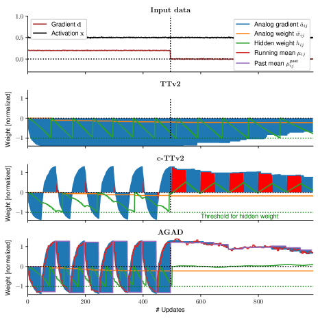
Figure 5: Sudden changes of gradient inputs. A long decay in the gradient matrix $\breve{A}$ for TTv2 is caused if input fluctuations are low, possibly biasing the weight update in situations of sparse gradient inputs (note that the hidden weight threshold for TTv2 is still hit after turning off net gradients at 500; green curve). Our new algorithms correct for this behavior. Parameters: as in Fig. 3.

In our new algorithms (c-TTv2 and AGAD), this artifact is not present, since the gradient update onto the hidden matrix is modulated by the chopper sign flips in both cases (Fig. A.3 and Fig. 5 lower panels). In particular, sparse gradients do not cause any residual weight update, because if $\breve{a}_{ij}$ is constant over multiple chopper periods it is treated as a bias that is subtracted out. The subtraction happens on the hidden matrix in case of c-TTv2 (notice the red and blue regions Fig. 5). For AGAD  a constant $\breve{a}_{ij}$ would not even be added to the hidden matrix because the dynamic reference point adjustment when changing the chopper phases removes any residual bias on-the-fly (Fig. 5 bottom).

4.4 Stochastic gradient descent on single linear layer

Next we test how the algorithm perform when using SGD. We consider training to program a linear layer with output $f_{i}(\mathbf{x})=\sum_{j=1}^{n}w_{ij}x_{j}$ to a given target weight matrix $\hat{W}$. We define the error as (mean squared deviation from the expected output by using the target weight $\hat{W}$)

$$L(\mathbf{x}|W,\hat{W})=\frac{1}{2m}\sum_{i}^{m}\Big{(}f_{i}(\mathbf{x})-\sum_{j=1}^{n}\hat{w}_{ij}x_{j}\Big{)}^{2}$$ (10)

Naturally, when minimizing the deviation (using SGD) and updating $W$, the error is minimized for $W=\hat{W}$ (assuming a full rank weight matrix). We set $\hat{W}$ to random values ${\cal N}(0,0.3)$ and use $x_{j}\sim{\cal N}(0,1)$ as inputs. We evaluate the different algorithms after convergence by the achieved weight error $\epsilon_{w}^{2}=\left\langle\left(w_{ij}-\hat{w}_{ij}\right)^{2}\right\rangle$, that is the standard deviation of the learned weights with the target weight. Fig. 6 shows the results for a $20\times 20$ weight matrix.

We compared the three algorithms (TTv2, c-TTv2, and AGAD) as well as plain in-memory SGD, where the gradient update is directly done on the weight $\breve{W}$ (Alg. 1). We explored the resilience to two parameter variations, (1) the standard deviation of the reference offset $\sigma_{r}$, as well as the number of device states $n_{\text{states}}$. As expected in case of no offset $\sigma_{r}=0$ and in agreement with the original study Gokmen (2021), the TTv2 algorithm works very well, vastly out performing in-memory SGD, in particular for small number of states (e.g. $\epsilon_{w}\approx 8\%$ vs $>25.0\%$, respectively, for 20 states and the very same target weight matrix; see Fig. 6AB). However, reference offset variations $\sigma_{r}>0$ critically affect the performance of TTv2. As soon as $\sigma_{r}=0.1$, weight errors increase significantly, posing challenges to current device materials and reference weight programming techniques.

Using choppers, on the other hand, improves the resiliency to offsets dramatically (Fig. 6CD). The c-TTv2 algorithm maintains the same weight error for a large offsets in particular when the number of states is small. Offsets in case of larger number of states are less well corrected, consistent with the problems of transients that increase for higher number of states (see Eq. 4). In case of AGAD, reference offset simply does not matter, as the reference is dynamically computed on-the-fly. Moreover, in contrast to c-TTv2, AGAD works equally well for higher number of states showing that transients are not problematic either. There is nevertheless a slight weight error increase for small number of states and small offsets in comparison to c-TTv2 which is likely due to some inaccuracies introduced by the on-the-fly estimation of the reference value.

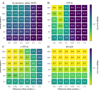
Figure 6: Weight programming error using different learning algorithms. Parameters: as in Fig. 3 except that $\sigma_{r}$ and $\delta_{w}$ is varied. Additionally we set $\sigma_{b}=0$ for $\breve{W}$ only (to not confound results for not being able to represent the target weight with $\breve{W}$). The target matrix, device-to-device variations, and inputs are fixed for each case for better comparison. Averaged over 3 runs.

4.5 DNN training experiments

Finally, we compared the different learning algorithms for actual DNN training. For better comparison, we use largely the same DNNs that was previously used to evaluate the earlier algorithms. These were a fully-connected DNN on MNIST Gokmen & Vlasov (2016), LeNet on MNIST Gokmen et al. (2017), and a two layer LSTM Gokmen et al. (2018); Gokmen (2021). We again trained the DNNs with difference reference offsets variations (see Fig. 7; see Sec. A.1 for details on the simulations) with the same challenging device model (see example device response traces for $n_{\text{states}}=20$ in Fig. A.1). The results are very consistent across the different DNNs and confirm the trends found in case of the weight programming of one layer (compare to Fig. 6): If the offsets are perfectly correct for, all algorithms fare very similarly. However, as expected, the impact of a reference offset is quite dramatic for TTv2  whereas c-TTv2 can largely correct for it until it becomes too large. On the other hand, AGAD is not affected by the offsets at all and typically shows best performance (Fig. 7B-D).

We found that even without offsets both new algorithms outperform the state-of-the-art TTv2. Moreover, now that the gradients are computed so well in spite of offsets and transients on $\breve{A}$, the second order effect of the not corrected SP on $\breve{W}$ is becoming prevalent. Indeed, the test error improves beyond the floating point (FP) test error for both c-TTv2 and AGAD when the SP of $\breve{W}$ is subtracted and thus corrected for (closed symbols), but increases somewhat if not (open symbols). AGAD shows better performance over c-TTv2 in particular for larger number of states (Fig. 7 A).

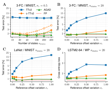
Figure 7: DNN training with different analog learning algorithms. SP of $\breve{W}$ is either corrected for (closed symbols) or not (open symbols with dashed lines). (A) Number of states versus test error with large reference offset variation $\sigma_{r}=0.5$. (B, C, D) Reference offset variation versus test error with $n_{\text{states}}=20$. DNNs: (A, B) 3-layer fully-connected DNN on MNIST (C) LeNet on MNIST (D) 2 layer LSTM on the War & Peace dataset.

5 Discussion

We have introduced two new learning algorithms for parallel in-memory training for crossbar arrays. All of these algorithms feature an essential ${\cal O}(n)$ time for calculating all operations required for the full SGD, namely forward, backward and update. In particular, the ${\cal O}(n^{2})$ calculation typically needed for the outer product during the weight matrix update is performed in ${\cal O}(1)$ since coincidence of a fixed number of pulses is used. The read of one column is fully parallel again ${\cal O}(1)$, while the additional digital compute operates on one column at a time and thus ${\cal O}(n)$.

Since c-TTv2 only introduces a sign flip, the computational complexity added to TTv2 is negligible. For AGAD the reference point is estimated on the fly which requires additional two digital weight matrices, their loading and storing thus add to the runtime. But since the additional operations still are performed on a column at a time, AGAD retains the ${\cal O}(n)$ complexity. One way to reduce the digital compute of AGAD, is to set $\beta=1$ and thus not compute any average over the recent past for the reference, which reduces the additional storage requirements to one matrix (only $\mu^{\text{past}}$), however, potentially introducing more noise.

The advantage of AGAD is that it improves performance for higher material states and makes the additional reference crossbar $\breve{R}$ obsolete, potentially reducing the unit cell complexity. Or alternatively to removing $\breve{R}$, this crossbar could now be used to store the SP of $\breve{W}$ and thus further improving accuracy with the same unit cell design.

We find that both c-TTv2 and AGAD push the boundary of in-memory training performance, while relaxing the number of state requirements on device materials. Indeed, we show that 20 states are now sufficient for training almost to floating point accuracy for our example DNNs, even in the presence of SP fluctuations or long-term transients.

Appendix A Appendix

A.1 DNN training simulation details

Here we describe the details of the DNN training simulations done in Fig. 7.

A.1.1 3-FC / MNIST

Here we use a 3-layer fully-connected DNN on the MNIST data set with sigmoid activations and hidden sizes of 255 and 127 as described in Gokmen & Vlasov (2016). For the analog MVM (forward and backward pass), we use essentially the standard settings of AIHWKit, which includes output noise (0.5 % of the quantization bin width), quantization and clipping (output range set to 20, output noise to 0.1, and input and output quantization to 8 bit). It uses the noise and bound management techniques as described in Gokmen et al. (2017). To adjust the output range to the DNN range, we add a learnable (scalar) floating point factor after each crossbar output, which is updated with standard momentum SGD (0.9 momentum term).

We train for 80 epochs and schedule the learning rate into 3 steps (35, 35, and 10 epochs), with reduction factor of 0.1. Starting learning rate is set to 0.05 (0.1 for floating point) and batch size is 10. Additionally, we set $n_{s}=1$ and $\gamma_{0}=10000$ and confirmed by a test run that it was a reasonable setting. We then run a grid of simulations and report the average test accuracy over the last 3 training epochs. The grid was the same for each condition, namely we simulated the settings of $\eta=0.05,0.1,0.2,0.5,1.0,2.0$. For each condition the best test error (averaged averaged over the last 3 epochs) is reported in the figure. The number of states was varied as indicated in the figure (see Fig. 7; parameter $\delta_{w}$). Other parameters are set as reported in Fig. 3. The chopper probability was set to $\rho=0.1$, where random switching was used for c-TTv2 and regular switching for AGAD as described in the algorithms (see Alg. 2 and Alg. 3, respectively).

For Fig. 7 A, we additionally varied the learning rate for each condition, and took the better one of the two $\lambda=0.05,0.025$. This resulted thus in 432 training simulations for this subplot alone.

A.1.2 LeNet / MNIST

A variant of the LeNet5 LeCun et al. (1998) model architecture, which contains 2-convolutional layers, 2-max-pooling layers, and 2-fully connected layers, trained on the MNIST dataset, is used here. The original LeNet5 model has 3-convolutional layers in its architecture. The model training is performed using the same setting of AIHWKit for the analog MVM (forward and backward pass) and the same device model as described above (Sec. A.1.1).

The model is trained for 60 epochs using a batch size of 8 and $\gamma_{0}=10000$. Different learning rate $\lambda$ values of 0.01, 0.02, 0.03, 0.04, and 0.05 are explored for $\sigma_{r}=0.0$, and the learning rate with the best test accuracy value is picked for each method under consideration, which resulted in the values $0.03$, $0.04$, and $0.04$ for TTv2, c-TTv2, and AGAD, respectively. The learning rate is scheduled into two steps (45 and 15 epochs) with a reduction factor of 0.10. The chopper probability (for the c-TTv2 and AGAD cases) is set to $\rho=0.1$, with random switching used for c-TTv2 and regular switching for AGAD.

The initial values of $\eta$ and $n_{s}$ are set to 1, and 1, respectively. Firstly, the value of $\eta$ is tuned until the best result is obtained. After that, the value of $n_{s}$ is also tuned. This tuning sequence is encouraged as $\eta$ has more influence on the model performance as measured using the test accuracy than $n_{s}$. The combination of these hyperparameter values that gives the best result is selected for all the methods. We find that $n_{s}=1$ works best for all methods and set $\eta$ to $0.05$, $0.1$ and $0.075$ for TTv2, c-TTv2, and AGAD, respectively. The test accuracy reported is the average over the test errors obtained after the last three training epochs.

The above obtained values of the $\eta$ and $n_{s}$ hyperparameters are then used to obtain the test accuracy for $\sigma_{r}=0.05,0.1,0.25,0.5,1.0$ respectively, and the resulting test accuracy is used to generate the plot in Fig. 7 C.

A.1.3 LSTM / War & Peace

We use a LSTM network composed of 2 stacked LSTM blocks with hidden vector size of 64 followed by a fully-connected layer, as described in Gokmen et al. (2018). We trained this network on the War and Peace (WP) novel. The dataset is split into a training set and test set with 2,933,246 and 325,000 character respectively, and a total vocabulary of 87 characters.

We trained the network using the AIHWKit for 100 epochs and schedule the learning rate into 3 steps (50, 40, and 20 epochs) with a reduction factor of 0.1. The starting learning rate is set to 0.1, batch size to 16, sequence length to 100, $\gamma_{0}=10000$ and chopper probability (for the c-TTv2 and AGAD cases) is set to $\rho=0.1$, with random switching used for c-TTv2 and regular switching for AGAD.

We run multiple simulations starting from the condition with reference offset variation $\sigma_{r}=0$. We explore different learning rate $\lambda=0.05,0.1,0.75$, different settings for $n_{s}=1,3$ and for $\eta=0.05,0.1,0.5,1.0$ and take the best combination of parameter for each algorithm. With the found parameter, we then perform the simulations for various reference offset variations and take the loss of the last epoch to generate the plot in Fig. 7 D.

A.2 Supplementary figures

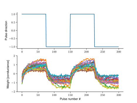
Figure A.1: Response traces of the simulated material used ($n_{\text{states}}=20$). Upper plot shows the pulsing pattern. Lower plot shows the response of 20 devices (colors). Note that significant asymmetry, device-to-device variation and cycle-to-cycle variation is present.

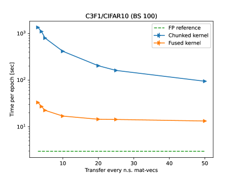
Figure A.2: Runtime of our improved CUDA kernel design for TTv2 (“Fused kernel”) in comparison to the existing “Chunked kernel” of the open source toolkit AIHWKit. The fused kernel is also used for our new algorithms c-TTv2 and AGAD. Here the time for one epoch on a standard small CNN on the CIFAR10 dataset Krizhevsky et al. (2009) is shown. The runtime is evaluated for different $n_{s}$ parameters (compare to Fig. 2). Note that our fused design improves the speed dramatically, from $>1000$ seconds to only $30$ seconds in the best case.

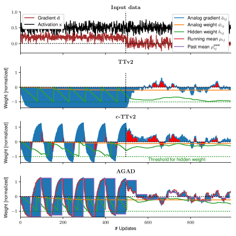
Figure A.3: Switching gradient input off causes the gradient matrix $\breve{A}$ to decay for TTv2 if input fluctuations are high. Our new algorithms also correctly stop the weight update in this case. Parameters: as in Fig. 3.

References

- Agarwal et al. (2016) Agarwal, S., Plimpton, S. J., Hughart, D. R., Hsia, A. H., Richter, I., Cox, J. A., James, C. D., and Marinella, M. J. Resistive memory device requirements for a neural algorithm accelerator. In 2016 International Joint Conference on Neural Networks (IJCNN), pp. 929–938. IEEE, 2016.
- Ambrogio et al. (2018) Ambrogio, S., Narayanan, P., Tsai, H., Shelby, R. M., Boybat, I., Nolfo, C., Sidler, S., Giordano, M., Bodini, M., Farinha, N. C., et al. Equivalent-accuracy accelerated neural-network training using analogue memory. Nature, 558(7708):60, 2018.
- Burr et al. (2017) Burr, G. W., Shelby, R. M., Sebastian, A., Kim, S., Kim, S., Sidler, S., Virwani, K., Ishii, M., Narayanan, P., Fumarola, A., et al. Neuromorphic computing using non-volatile memory. Advances in Physics: X, 2(1):89–124, 2017.
- Enz & Temes (1996) Enz, C. C. and Temes, G. C. Circuit techniques for reducing the effects of op-amp imperfections: autozeroing, correlated double sampling, and chopper stabilization. Proceedings of the IEEE, 84(11):1584–1614, 1996.
- Fick et al. (2022) Fick, L., Skrzyniarz, S., Parikh, M., Henry, M. B., and Fick, D. Analog matrix processor for edge ai real-time video analytics. In 2022 IEEE International Solid-State Circuits Conference (ISSCC), volume 65, pp. 260–262. IEEE, 2022.
- Frascaroli et al. (2018) Frascaroli, J., Brivio, S., Covi, E., and Spiga, S. Evidence of soft bound behaviour in analogue memristive devices for neuromorphic computing. Scientific reports, 8(1):1–12, 2018.
- Fusi & Abbott (2007) Fusi, S. and Abbott, L. Limits on the memory storage capacity of bounded synapses. Nature neuroscience, 10(4):485–493, 2007.
- Gokmen (2021) Gokmen, T. Enabling training of neural networks on noisy hardware. Frontiers in Artificial Intelligence, 4:1–14, 2021.
- Gokmen & Haensch (2020) Gokmen, T. and Haensch, W. Algorithm for training neural networks on resistive device arrays. Frontiers in Neuroscience, 14, 2020.
- Gokmen & Vlasov (2016) Gokmen, T. and Vlasov, Y. Acceleration of deep neural network training with resistive cross-point devices: Design considerations. Frontiers in neuroscience, 10:333, 2016.
- Gokmen et al. (2017) Gokmen, T., Onen, M., and Haensch, W. Training deep convolutional neural networks with resistive cross-point devices. Frontiers in neuroscience, 11:538, 2017.
- Gokmen et al. (2018) Gokmen, T., Rasch, M. J., and Haensch, W. Training LSTM networks with resistive cross-point devices. Frontiers in neuroscience, 12:745, 2018.
- Gong et al. (2022) Gong, N., Rasch, M., Seo, S.-C., Gasasira, A., Solomon, P., Bragaglia, V., Consiglio, S., Higuchi, H., Park, C., Brew, K., et al. Deep learning acceleration in 14nm cmos compatible reram array: device, material and algorithm co-optimization. In IEEE International Electron Devices Meeting, 2022.
- Haensch et al. (2019) Haensch, W., Gokmen, T., and Puri, R. The next generation of deep learning hardware: Analog computing. Proceedings of the IEEE, 107(1):108–122, 2019.
- Jain et al. (2019) Jain, S. et al. Neural network accelerator design with resistive crossbars: Opportunities and challenges. IBM Journal of Research and Development, 63(6):10–1, 2019.
- Khaddam-Aljameh et al. (2021) Khaddam-Aljameh, R., Stanisavljevic, M., Mas, J. F., Karunaratne, G., Braendli, M., Liu, F., Singh, A., Müller, S. M., Egger, U., Petropoulos, A., et al. Hermes core–a 14nm cmos and pcm-based in-memory compute core using an array of 300ps/lsb linearized cco-based adcs and local digital processing. In 2021 Symposium on VLSI Circuits, pp. 1–2. IEEE, 2021.
- Kim et al. (2019) Kim, H., Rasch, M. J., Gokmen, T., Ando, T., Miyazoe, H., Kim, J.-J., Rozen, J., and Kim, S. Zero-shifting technique for deep neural network training on resistive cross-point arrays. arXiv preprint arXiv:1907.10228, 2019.
- Kingma & Ba (2014) Kingma, D. P. and Ba, J. Adam: A method for stochastic optimization. arXiv preprint arXiv:1412.6980, 2014.
- Krizhevsky et al. (2009) Krizhevsky, A., Hinton, G., et al. Learning multiple layers of features from tiny images. 2009.
- LeCun et al. (1998) LeCun, Y., Bottou, L., Bengio, Y., and Haffner, P. Gradient-based learning applied to document recognition. Proceedings of the IEEE, 86(11):2278–2324, 1998.
- Nandakumar et al. (2018) Nandakumar, S. R., Le Gallo, M., Boybat, I., Rajendran, B., Sebastian, A., and Eleftheriou, E. Mixed-precision architecture based on computational memory for training deep neural networks. In 2018 IEEE International Symposium on Circuits and Systems (ISCAS), pp. 1–5, 2018.
- Nandakumar et al. (2020) Nandakumar, S. R., Le Gallo, M., Piveteau, C., Joshi, V., Mariani, G., Boybat, I., Karunaratne, G., Khaddam-Aljameh, R., Egger, U., Petropoulos, A., Antonakopoulos, T., Rajendran, B., Sebastian, A., and Eleftheriou, E. Mixed-precision deep learning based on computational memory. Frontiers in Neuroscience, 14, 2020.
- Narayanan et al. (2021) Narayanan, P., Ambrogio, S., Okazaki, A., Hosokawa, K., Tsai, H., Nomura, A., Yasuda, T., Mackin, C., Lewis, S., Friz, A., et al. Fully on-chip mac at 14nm enabled by accurate row-wise programming of pcm-based weights and parallel vector-transport in duration-format. In 2021 Symposium on VLSI Technology, pp. 1–2. IEEE, 2021.
- Onen et al. (2022) Onen, M., Gokmen, T., Todorov, T. K., Nowicki, T., Del Alamo, J. A., Rozen, J., Haensch, W., and Kim, S. Neural network training with asymmetric crosspoint elements. Frontiers in artificial intelligence, 5, 2022.
- Paszke et al. (2019) Paszke, A., Gross, S., Massa, F., Lerer, A., Bradbury, J., Chanan, G., Killeen, T., Lin, Z., Gimelshein, N., Antiga, L., et al. Pytorch: An imperative style, high-performance deep learning library. Advances in neural information processing systems, 32, 2019.
- Rasch et al. (2021) Rasch, M., Moreda, D., Gokmen, T., Gallo, M. L., Carta, F., Goldberg, C., Maghraoui, K. E., Sebastian, A., and Narayanan, V. A flexible and fast pytorch toolkit for simulating training and inference on analog crossbar arrays. IEEE International Conference on Artificial Intelligence Circuits and Systems (AICAS), pp. 1–4, 2021.
- Sebastian et al. (2020) Sebastian, A., Le Gallo, M., Khaddam-Aljameh, R., and Eleftheriou, E. Memory devices and applications for in-memory computing. Nature Nanotechnology, 15:529–544, 2020.
- Steinbuch (1961) Steinbuch, K. Die Lernmatrix. Kybernetik, 1(1):36–45, 1961.
- Sze et al. (2017) Sze, V., Chen, Y.-H., Yang, T.-J., and Emer, J. S. Efficient processing of deep neural networks: A tutorial and survey. Proceedings of the IEEE, 105(12):2295–2329, 2017.
- Wan et al. (2022) Wan, W., Kubendran, R., Schaefer, C., Eryilmaz, S. B., Zhang, W., Wu, D., Deiss, S., Raina, P., Qian, H., Gao, B., et al. A compute-in-memory chip based on resistive random-access memory. Nature, 608(7923):504–512, 2022.
- Xue et al. (2021) Xue, C.-X., Chiu, Y.-C., Liu, T.-W., Huang, T.-Y., Liu, J.-S., Chang, T.-W., Kao, H.-Y., Wang, J.-H., Wei, S.-Y., Lee, C.-Y., et al. A cmos-integrated compute-in-memory macro based on resistive random-access memory for ai edge devices. Nature Electronics, 4(1):81–90, 2021.
- Yang et al. (2013) Yang, J. J., Strukov, D. B., and Stewart, D. R. Memristive devices for computing. Nature nanotechnology, 8(1):13, 2013.
- Yao et al. (2020) Yao, P., Wu, H., Gao, B., Tang, J., Zhang, Q., Zhang, W., Yang, J. J., and Qian, H. Fully hardware-implemented memristor convolutional neural network. Nature, 577(7792):641–646, 2020.
- Zahoor et al. (2020) Zahoor, F., Azni Zulkifli, T. Z., and Khanday, F. A. Resistive random access memory (rram): an overview of materials, switching mechanism, performance, multilevel cell (mlc) storage, modeling, and applications. Nanoscale research letters, 15(1):1–26, 2020.