Contact geometry in peeling a thin solid from a liquid

Torque-free peeling: lifting a thin partially-wetting solid off a liquid surface

Torque-free peeling: the triple-phase contact line at a bendable sheet

Peeling without local torque: how a bendable sheet detaches from a liquid

Peeling from a liquid

Abstract

We establish the existence of a cusp in the curvature of a solid sheet at its contact with a liquid subphase. We study two configurations in floating sheets where the solid-vapor-liquid contact line is a straight line and a circle, respectively. In the former case, a rectangular sheet is lifted at its edge, whereas in the latter a gas bubble is injected beneath a floating sheet. We show that in both geometries the derivative of the sheet’s curvature is discontinuous. We demonstrate that the boundary condition at the contact is identical in these two geometries, even though the shape of the contact line and the stress distribution in the sheet are sharply different.

The peel test is an extensively used method to measure the strength of adhesion of a sheet to a substrate. The test, schematically depicted in Fig. 1 panels B1-D1, is usually based on measuring the force required to separate the sheet from the substrate. In fact, a direct measurement of the shape of the sheet near the separation front, performed in a classic 1930 study by Obreimoff on a freshly cleaved mica [1], has been arguably the earliest attempt to determine the surface energy of solids. In this test the peeled-off part of the sheet has a parabolic shape while the adhered portion of the sheet remains flat. The discontinuity in curvature, $\kappa(s)$, where $s$ is the distance to the contact line, reflects a highly-localized torque (on the scale of the sheet’s thickness) that is exerted by the rigid substrate on the peeled-off sheet. The presence of a singular torque underlies the celebrated Obreimoff’s law:

peeling off rigid substrate:

$$[[\kappa]]=\sqrt{2}/\ell_{bc}$$ (1)

$$\text{where:}\ \ \ell_{bc}\equiv\sqrt{B/T}\ .$$ (2)

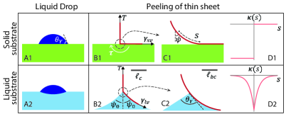
Figure 1: (A1) Liquid drop on a rigid solid substrate. (A2) Liquid drop on a liquid substrate. (B1, C1) Thin sheet peeling from a solid substrate. (B2, C2) Thin sheet peeling from a liquid substrate. Panels B1 and B2 are at the capillary length scale, $\ell_{c}$, while panels C1 and C2 are zoomed in to the bendo-capillary scale $\ell_{bc}$. (D1) Curvature near the contact line for thin sheet peeling from a solid substrate [1]. (D2) Continuous curvature for a thin sheet peeled from a liquid substrate characterized by a cusp at the contact line.

Here, $[[\kappa]]=\kappa(s\to 0^{+})-\kappa(s\to 0^{-})$ denotes the jump in curvature at $s=0$ in the (otherwise continuous) curvature, $B$ the bending modulus of the sheet, and $T$ the tension in the sheet (attributed by Obreimoff to its surface energy with the ambient phase). In Eq. (1), we follow a terminology used in studies of elasto-capillary phenomena that involve slender bodies at fluid interfaces, where Eq. (2) defines a “bendo-capillary” length, $\ell_{bc}$, over which bending and tensile forces are comparable.

In this paper we study peeling of a thin solid sheet from a liquid subphase, schematically depicted in Fig. 1 panels B2-D2. In contrast to a rigid solid, no localized torque is exerted by the liquid subphase at the contact line. Consequently, the curvature is continuous, and the only discontinuity possible at mechanical equilibrium is of the derivative $\kappa^{\prime}(s)$. The analogue of Obreimoff’s law for peeling a solid sheet off a liquid subphase becomes:

peeling off liquid subphase:

$$[[\kappa]]=0\ \ ;\ \ [[\kappa^{\prime}]]=\sin\theta_{Y}/\ell_{bc}^{2}\ ,$$ (3)

where $\ell_{bc}$ is defined through Eq. (2) with $T=\gamma_{\ell v}$, and

$$\theta_{Y}=\cos^{-1}{\color[rgb]{0,0,0}\left[{(\gamma_{sv}-\gamma_{s\ell})}/{\gamma_{\ell v}}\right]}$$ (4)

is the Young-Laplace-Dupré (YLD) angle, which is determined by the mutual surface energies between the liquid, solid, and ambient (vapor) phase. While Eq. (3) has been noted already in a one-dimensional (1D) model system of “bendable” partial wetting phenomena [2], whereby a finite liquid volume is deformed upon making contact with a thin solid along a straight line [3], our study is the first, to our knowledge, to confirm it experimentally and employ it in realistic peeling geometries in 1D as well as in 2D (i.e. circular contact line). Determining a discontinuity in the derivative of the curvature (which amounts to the third derivative of a profile extracted from an image) is challenging, as noise-averaging smooths over the crucial localized feature we seek to identify. Indeed, we are not aware of any direct experimental study of a discontinuity in second derivative in the solid-peeling case.

As illustrated in Fig. 1, the difference between the original Obreimoff law for peeling off a rigid substrate (Eq. (1)) and its modified version for a liquid bath (Eq. (3)), parallels the difference between the contact angle laws for solid-liquid-vapor (YLD) and a liquid-liquid-vapor (Neuman). In both scenarios – partial wetting of a finite liquid volume (panels A) versus peeling off a substrate (panels B-D) – the difference between a rigid solid substrate (top row) and a liquid subphase (bottom row) stems from the fact that a liquid bath cannot support normal load without deforming its surface. However, in contrast to the contact angle problem on either a liquid or solid subphase, where the only length scale is the size of the liquid drop, the geometry of a sheet peeled-off from a liquid sub-phase consists of multiple scales. Zooming in close to the contact line at a size scale $\ll\ell_{bc}$ (panel C2) reveals a geometry that is almost indistinguishable from the vicinity of a contact on a thick rigid body of the same material (panel A1), except for a discontinuity of the $3^{rd}$ derivative of the surface, which is reflected (panel D2) by a cusp in the curvature $\kappa(s)$. Zooming out to a size that is $\gg\ell_{bc}$ yet $\ll\ell_{c}=\sqrt{\gamma_{\ell v}/\rho g}$ (panel B2) one observes a liquid meniscus dominated by a balance of surface tension and gravity (Young-Laplace equation), which terminates at a kink, as if the curvature was diverging. This multi-scale scenario is valid only if the sheet is sufficiently thin, such that $\ell_{bc}\ll\ell_{c}$, or more generally:

$$\epsilon\ll 1\ \ ,\ \ \text{where}\ \ \epsilon\equiv(\ell_{bc}/L_{out})^{2}\ .$$ (5)

Here, $L_{out}$ is an “outer” scale, at which the curvature approaches an asymptotic value, which is $\ll\ell_{bc}^{-1}$. For the example depicted in Fig. 1D2 , where $L_{out}=\ell_{c}$, the ratio $\epsilon={\color[rgb]{0,0,0}\rho gB/\gamma_{\ell v}^{2}}$ is akin to the “softness” parameter that was defined in Ref. [4].

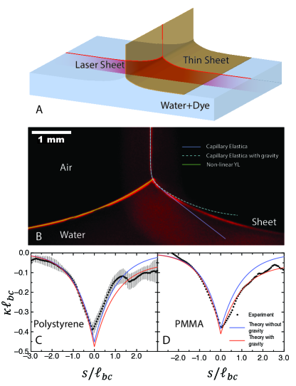
Figure 2: 1D geometry. (A) Schematic of experimental setup. The upper edge of the sheet is held at a fixed, controllable height. (B) A typical image of the sheet profile (Polystyrene, thickness $t=2$ $\mu$m corresponding to $\ell_{bc}=0.2$ mm). Superimposed on the image are solutions of the non-linear Young-Laplace equation [5] (solid green line), the capillary elastica Eq. (15) (solid blue curve), and the capillary elastica with gravity correction (dashed cyan curve). The curvature $\kappa(s)$ for (C) Polystyrene sheet ($t=2$ $\mu$m) with estimated statistical error bars and (D) PMMA sheet ($t=2$ $\mu$m). Filled black circles, blue and red lines represent data, theoretical prediction from capillary elastica and capillary elastica with gravity correction, respectively.

1D translationally symmetric geometry:

We first address an effectively one-dimensional (1D) geometry, where the deformed sheet is characterized by translational symmetry along the direction parallel to the contact line, as shown schematically in the bottom part of Fig. 1B and Fig. 2A. Such a 1D set-up is realized in a floating, rectangular thin sheet, which is peeled off by exerting a vertical force $T_{peel}$ along one of its short edges. As we noted above, when observed at intermediate scales, $\ell_{bc}\ll|s|\lesssim\ell_{c}$, the sheet appears to have a cusp at the contact line; furthermore, the mechanical equilibrium shape is characterized by reflection symmetry of the two sides of the surface (sheet-covered and liquid-vapor) around the vertical line [6]. The reflection symmetry indicates that the tension in the wet part of the sheet is identical to the liquid-vapor surface tension, $\gamma_{\ell v}$, and force balance at the contact line thus determines the force, $T_{peel}$, the opening angle, $2\psi_{0}$, of the apparent cusp, and the height, $H_{0}$, of the contact line over the liquid bath level:

$$T_{peel}=\gamma_{\ell v}(1+\cos\theta_{Y})=2\gamma_{\ell v}\cos\psi_{0}$$ (6)

$$\Longrightarrow\ \psi_{0}\approx\cos^{-1}[\cos^{2}\frac{\theta_{Y}}{2}]\ \ ,\ \ H_{0}\approx f(\psi_{0})\ell_{c}\ ,$$ (7)

where the function $f(\psi_{0})$ is found by solving the (nonlinear) Young-Laplace equation [5], such that $f\!\approx\!(\pi/2-\psi_{0})$ for $\psi_{0}\to\pi/2$ and $f\!\approx\!\sqrt{2}$ for $\psi_{0}\to 0$. The shape of the whole sheet is described by a planar vector, $\vec{X}(s)\!=\!x(s)\hat{i}\!+\!y(s)\hat{j}$, where $s$ is an arclength parameter, and is conveniently described through the angle, $\psi(s)$, between the tangent vector, $\vec{X}^{\prime}$ and the downward vertical $-\hat{y}$:

$$x^{\prime}(s)=\sin\psi\ \ ;\ \ y^{\prime}(s)=\cos\psi\ \ ;\ \ \text{and}\ \ \kappa(s)=\psi^{\prime}\ .$$ (8)

At mechanical equilibrium, the shape satisfies the capillary elastica, which expresses normal force balance [2, 7]:

$$B\left[\kappa^{\prime\prime}+\frac{\kappa^{3}}{2}\right]-T(s)\kappa=-P(s){\color[rgb]{0,0,0}+}\gamma_{\ell v}\sin\theta_{Y}\delta_{d}(s)$$

$$P(s)\!=\!\left\{\begin{array}[]{ll}0&s<0\\ -\rho gy(s)&s>0\end{array}\right.\quad T(s)=\left\{\begin{array}[]{ll}T_{peel}&s<0\\ \gamma_{\ell v}&s>0\end{array}\right.$$ (13)

Here, $P(s)$ is the hydrostatic pressure exerted by the liquid bath on the wet portion of the sheet, $s>0$ (where $\rho$ and $g$ are, respectively, the liquid density and gravity acceleration), $T(s)$ is the tension in the sheet, and $\gamma_{\ell v}\sin\theta_{Y}$ is the normal force exerted by the liquid-vapor interface at the contact line. In a 1D geometry at mechanical equilibrium (and absence of external shear forces) the tension $T(s)$ satisfies $\partial_{s}T=0$, and is consequently constant in the dry part ($s<0$), where it is given by the force $T_{peel}$ exerted by the peeler, and in the wet part ($s>0$), where it is given by the liquid-vapor surface that pulls on the edge of the floating sheet.

Integrating both sides of Eq. (13) over an infinitesimal neighborhood of the contact line, $s=0$, we obtain:

$$B[[\kappa^{\prime}]]={\color[rgb]{0,0,0}\gamma_{\ell v}\sin\theta_{Y}}\ ,$$ (14)

and integrating once more across the contact line we obtain $[[\kappa]]=0$, thereby establishing Eq. (3) .

On each side of the contact line, the profile of the sheet is determined by the capillary elastica (13) which is a nonlinear $3^{rd}$ order equation for $\psi(s)$, whose solution requires 3 boundary conditions (BCs). Thus, in addition to Eqs. (14,3), 4 other BCs must be specified. To obtain these, we non-dimensionalize length by defining $\bar{s}=s/\ell_{bc}$ and $\bar{\kappa}=\kappa\ell_{bc}$, and consider Eq. (13), in the singular limit $\epsilon\to 0$ (see SI). At $O(\epsilon^{0})$, we obtain 2 “outer” BCs at each side of the contact line. At $\bar{s}\to-\infty:\ \psi\to 0,\bar{\kappa}\to 0$, and at $\bar{s}\to+\infty:\ \psi\to\psi_{0},\bar{\kappa}\to 0$, and the corresponding (exact) solution of Eq. (13) at $O(\epsilon^{0})$ is given by:

$$\bar{s}\! > \!0\!:\ \bar{\kappa}\!=\!-2\ \text{sech}(\bar{s}\!+\!\bar{s}_{w})\ ,$$ (15)

$$\bar{s}\! < \!0\!:\ \bar{\kappa}\!=\!-2\sqrt{r}\ \text{sech}{[(\bar{s}\!+\!\bar{s}_{d}}){\sqrt{r}]}\ ,r\equiv\frac{T_{peel}}{\gamma_{\ell v}}=2\cos\psi_{0}\ ,$$

$$\text{where:}\ \ \bar{s}_{w}=\cosh^{-1}(a)\ ;\ \bar{s}_{d}=-\cosh^{-1}(a\sqrt{r})/\sqrt{r}\ ;\$$

$$a=(2/\sin\theta_{Y})\sqrt{b+\sqrt{b^{2}-1}}\ ;\ b=1+r\ .$$ (16)

In the SI, we describe a next-order, $O(\epsilon^{1})$ solution, which incorporates the gravity effect on the sheet curvature and is useful for comparison with experimental data.

The setup employed to study the problem experimentally is illustrated schematically in Fig.2 A. Thin sheets of Polystyrene (Polymer source P10453-S, $Mw=97.6$ kDa, Young’s modulus = 3.5 GPa) and PMMA (Aldrich 182265, $Mw\sim 996$ kDa, Young’s modulus = 3 GPa) of 1-2 $\mu m$ thickness are prepared by spin-coating on glass slides. Rectangles of 20 mm width and 60 mm length are cut from these films and floated on the surface of a water bath ($\ell_{c}$=2.7 mm). The long end of the film is then lifted out of the water surface by using a triangular hanger made up of graphite rods of diameter 0.7 mm (pencil leads). Sheet illumination produced from a green laser (wavelength 532 nm) is used to illuminate the interface near the contact line for imaging. A dye (Rhodamine-B) is dissolved in water in miniscule amount rendering both sides of the interface fluorescent. The interface is imaged using a DSLR camera (Nikon D5300) with a macro-lens and a long pass filter to admit only the fluorescent light. The laser sheet is positioned near the center of the film which is many $\ell_{c}$ away from the ends of the contact line. In this configuration end-effects near the edges of the sheet are negligible and the film profile can be assumed to be 2D. A typical image obtained from the setup is shown in Fig. 2B. The resolution of the imaging setup (1 pixel $\sim 1$ $\mu m$) is typically much smaller than $\ell_{bc}$, which is approximately 0.2 mm for the films used. Superimposed on the image are the solution of the Young-Laplace equation [5] as green solid curve for the liquid-vapor interface (left to the contact line), the solution to the capillary elastica without gravity as a blue solid curve, and the solution of the capillary elastica with gravity as the dashed cyan curve.

A gradient method is used to detect the interface and to obtain its $(x,y)$ coordinates along the film from the images, and $\kappa(s)$, the curvature vs. arclength is computed from:

$$\kappa(x)\!=\!\frac{y^{\prime\prime}(x)}{(1+y^{\prime}(x)^{2})^{3/2}}\ ;\ s(x)\!=\!\int_{0}^{x}\!\!\!\sqrt{1+y^{\prime}(x)^{2}}dx\ .$$ (17)

On computing derivatives from experimental data, the noise in the data gets amplified, which usually necessitates some form of smoothing. However, traditional smoothing methods will suppress any cusp in $\kappa(s)$. We therefore developed the algorithm described below to extract $\kappa(s)$ from the $(x,y)$ data.

We divide the whole data set into intervals of length $\Delta\sim\ell_{bc}$. We construct a sample of this data by choosing one data point from each interval randomly with a uniform probability distribution. We can estimate the position of the contact line from the images with a much higher accuracy and precision of a few pixels. We add to the data sample a contact-line location selected randomly with a Gaussian probability distribution centered at the estimated position of the contact line and having a width equal to the estimated error. A spline function of order $3$ made up of Hermite polynomials is generated using this sampling of data points and the curvature is computed on this spline function at roughly every $10^{th}$ point of the original data set. The process is repeated a large number of times (about twice the number of data points in each interval), selecting a different sampling of data points, such that the whole data set is adequately represented. The curvature profiles obtained from individual data samples are averaged to obtain the final $\kappa(s)$ curve. This procedure allows noise-averaging and use of the full data set without spatial averaging that would smooth the putative curvature cusp.

The black filled circles in Fig. 2C-D show $\kappa(s)$ as determined by the above described method for a polystyrene (PS) and a PMMA film of thickness $t=2$ ${\color[rgb]{0,0,0}\mu}$m, respectively. Superimposed on the experimental data are the theoretical predictions obtained by solving the capillary elastica equation neglecting gravity and capillary elastica with gravity in blue and red lines respectively. We notice that the theoretical predictions match the experimental data quite well and show a clear cusp at $s=0$.

When gravity is neglected, the only input parameter required to solve the capillary elastica is $\psi_{0}$; however, this can be directly measured from the water-air interface near the contact line in the image and is found to be $48.8^{\circ}$ and $40.0^{\circ}$ for the PS and the PMMA films in Fig. 2C and 2D, respectively. In order to generate the solution of the capillary elastica with gravity, in addition to $\psi_{0}$, we require the value of $\epsilon=(\ell_{bc}/\ell_{c})^{2}$, which is already known. Thus, there is no fitting parameter involved in computing the theory curves.

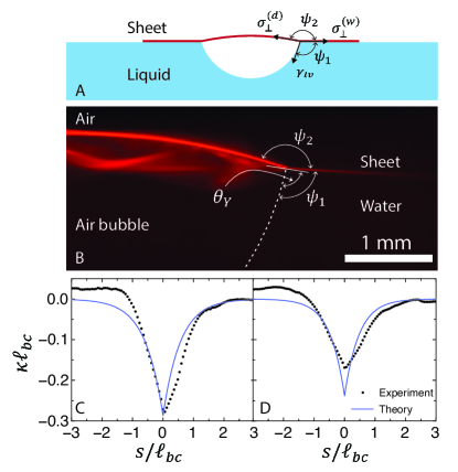
Figure 3: 2D axially-symmetric geometry. (A) The setup consists of a thin sheet floating on water with an air bubble underneath. (B) A typical image of the sheet profile (Polystyrene, thickness $t=2$ ${\color[rgb]{0,0,0}\mu}$m). The dashed white curve is a circle fitted to the air bubble, and the white solid line is tangent to the sheet profile at the contact line. The curvature $\kappa(s)$ for air bubble of radius (C) $4.1$ mm and (D) $3.1$ mm.

Axial geometry:

While the 1D geometry of the setup described in Fig. 2 presents a simple setting to discuss the boundary conditions at the contact line, the curvature cusp predicted by Eq. (3) appears in various other settings that are often encountered in elasto-capillary phenomena. One example is the axially-symmetric geometry of a thin sheet floating on water with an air-bubble of volume $V$ underneath it, as shown schematically in Fig. 3A. In contrast to the 1D geometry, which is free of Gaussian curvature and whose mechanical equilibrium is thus described everywhere by a planar curve $\vec{X}(s)$ that solves the elastica, Eq. (13), the axial geometry in Fig. 2 is characterized by Gaussian curvature, and thus involves a nontrivial variation of both radial and hoop components of the stress and curvature tensors with radial distance $r$. Hence, the shape of the sheet must be described by a surface $\vec{X}(r,\theta)$, that is obtained by solving the Föppl-von Kármán (FvK) equations [9, 10], and is furthermore susceptible to radial wrinkling instability due to hoop compression exhibited by an axisymmetric solution [11, 12]. Nevertheless, as long as the bendo-capillary length is sufficiently small, (namely, $\epsilon\ll 1$, where $L_{out}$ in Eq. (5) is now given by the drop’s radius and/or the capillary length $\ell_{c}$), the dominant terms in the curvature and stress tensors in the vicinity of the contact line are the radial components, and consequently the normal force balance is given by an equation similar to Eq. (13):

$$B\left(\kappa_{\perp}^{\prime\prime}+{\kappa_{\perp}^{3}}/2\right)-\sigma_{\perp}\kappa_{\perp}=-\gamma_{\ell v}\sin\theta_{Y}\delta_{d}(s)\ ,$$ (18)

where $\kappa_{\perp}(s),\sigma_{\perp}(s)$ are principal components of the curvature and stress tensors, respectively, along the radial direction, perpendicular to the contact line, and $s$ is the distance from the contact line. In the preceding analysis we neglected in Eq. (18) the sub-dominant hydrostatic pressure term; for similar reasons we ignore spatial variation of $\sigma_{\perp}$ on each side of the contact line. Once again, considering an infinitesimal vicinity of the contact line, we note that tangential force balance yields:

$$\sigma_{\perp}^{(d)}=\gamma_{lv}\cos\theta_{Y}+\sigma_{\perp}^{(w)}\$$ (19)

(where superscripts refer to the dry and wet sides), to which we refer as YLD equation, and integration of Eq. (18) yields the jump condition, Eq. (3).

The validity of Eq. (18) hinges upon scale separation, namely $\epsilon\ll 1$, where the ratio $\epsilon$ is given by Eq. (5), with

$$\ell_{bc}\longrightarrow\ell_{bc}^{*}\equiv\sqrt{B/\sigma_{\perp}}\ \ ;\ \ L_{out}\longrightarrow\min\{\ell_{C},V^{1/3}\}$$ (20)

(see SI and Ref. [10]). Similarly to our analysis of Eq. (13), the $O(\epsilon^{0})$ boundary conditions for Eq. (18) consist of vanishing curvature away from the contact line (i.e. $\bar{\kappa},\bar{\kappa}^{{}^{\prime}}\sim O(\epsilon,\sqrt{\epsilon})$, respectively). However, in contrast to the simpler 1D geometry, finding the asymptotic tangent angle $\psi_{1,2}$ at the two sides of the contact line, as well as the stress $\sigma_{\perp}$ in its vicinity, requires one to solve the FvK equations – a nonlinear set of partial differential equations – in the singular limit of vanishing bending rigidity (known as “membrane limit” or “tension field theory”). Rather than following such a theoretical track (á la Refs. [9, 10]), we note that force balance on an “intermediate box” of size $\ell_{bc}^{*}\ll\ell\ll L_{out}$, around the contact line (see Fig. 3B). implies that, at $O(\epsilon^{0})$:

$$\sigma_{\perp}^{(d)}=-\sigma_{\perp}^{(w)}\cos\psi_{2}-\gamma_{lv}\cdot\cos(\psi_{1}+\psi_{2})$$

$$\sigma_{\perp}^{(w)}\sin\psi_{2}=-\gamma_{lv}\sin(\psi_{1}+\psi_{2})$$ (21)

(often called “Neuman contact” [13]), which implies that $\gamma_{lv}$ and the two asymptotic angles, $\psi_{1},\psi_{2}$, uniquely determine the in-plane stress in the sheet, $\sigma_{\perp}^{(w)},\sigma_{\perp}^{(d)}$, near the contact line, and consequently the YLD angle $\theta_{Y}$ by Eq. (19). Note that for the 1D peeling geometry considered earlier, $\sigma_{\perp}^{(w)}=\gamma_{lv}$, whereas $\psi_{1}=2\psi_{0}$ and $\psi_{2}=\pi-\psi_{0}$, such that Eqs. (19, 21) reduce to Eq. (6).

An air bubble released within the fluid, forms a bubble beneath the sheet. To image the contact line between bubble, sheet and water subphase, a vertical plane passing through the center of the setup is imaged using a laser-sheet fluorescence method similar to the one illustrated in Fig. 2. A typical image of the sheet profile obtained from these experiments is shown in Fig. 3B. A bright-field image is taken after the fluorescence image, and used to obtain the profile of the air-bubble. The dashed white curve in Fig. 3B represents a circle fitted to the air-bubble shape. Figures 3C-D show $\kappa(s)$ for bubble radii $R=4.1$ mm and $R=3.1$ mm, respectively. The data demonstrate that in this geometry too, the curvature has a cusp near $s=0$, representing a discontinuity in the derivative of the curvature.

Problems such as the 1D and axial peeling geometries in highly-bendable sheets typically come in two parts with a big separation in length scale - an “inner”, bending-dominated region of size $\ell_{bc}^{*}$ that is governed by the elastica, and an “outer” region, where the shape and stress are independent of bending rigidity. At the innermost part of the bending-dominated zone is the purely local effect that we have established in this article, with a discontinuity in the gradient of the curvature in the vicinity of the contact line, $[[\kappa_{\perp}^{\prime}]]$, which is determined purely by material parameters ($B,\gamma_{lv},\theta_{Y}$). This discontinuity affects the bending-dominated region as a “near-field” boundary condition to the elastica problem, but a complete solution of the elastica requires also a “far-field” boundary condition, which is obtained by matching with the outer, bending-independent problem. In the cases we considered, this matching condition is expressed through a single parameter, the asymptotic angle $\psi_{0}$ in Fig. 1 or equivalently $\psi_{2}=\pi-\psi_{0}$ in Fig. 3. Neglecting the bending-dominated region altogether (as was proposed in [14] for sufficiently thin sheets) leads to an error in the region close to the contact. Neglecting the curvature discontinuity at the contact line (as in the elastica problem for 1D delamination studied by [15]) can also lead to an error in the predicted shape, and when tension is small, the error may span a large portion of the sheet. In conclusion, we note that the geometry-independent nature of the discontinuity, $[[\kappa_{\perp}^{\prime}]]$, provides the basis for a robust method for determining contact angles both at and away from equilibrium.

References

- Obreimoff [1930] J. Obreimoff, The splitting strength of mica, Proceedings of the Royal Society of London. Series A, Containing Papers of a Mathematical and Physical Character 127, 290 (1930).
- Neukirch et al. [2013] S. Neukirch, A. Antkowiak, and J.-J. Marigo, The bending of an elastic beam by a liquid drop: a variational approach, Proceedings of the Royal Society A: Mathematical, Physical and Engineering Sciences 469, 20130066 (2013).
- Py et al. [2007] C. Py, P. Reverdy, L. Doppler, J. Bico, B. Roman, and C. N. Baroud, Capillary origami: spontaneous wrapping of a droplet with an elastic sheet, Physical review letters 98, 156103 (2007).
- Huang et al. [2010] J. Huang, B. Davidovitch, C. D. Santangelo, T. P. Russell, and N. Menon, Smooth cascade of wrinkles at the edge of a floating elastic film, Physical Review Letters 105, 2 (2010), 0901.2892 .
- Anderson et al. [2006] M. L. Anderson, A. P. Bassom, and N. Fowkes, Exact solutions of the Laplace-Young equation, Proceedings of the Royal Society A: Mathematical, Physical and Engineering Sciences 462, 3645 (2006).
- Kumar et al. [2020] D. Kumar, T. P. Russell, B. Davidovitch, and N. Menon, Stresses in thin sheets at fluid interfaces, Nature Materials 19, 690 (2020).
- Kozyreff et al. [2022] G. Kozyreff, B. Davidovitch, S. G. Prasath, G. Palumbo, and F. Brau, Wetting of an elastic sheet subject to external tension (2022), arXiv:2201.10925 [cond-mat.soft] .
- Note [1] A higher-order effect, which cannot be accounted by Eq. (13), it the small torque exerted by the liquid-vapor interface on the sheet if they are not perpendicular at the contact line (i.e. ). This localized torque is explicitly proportional to the thickness, yielding a discontinuity of the curvature , whose effect on the shape is negligible , i.e. for .
- Schroll et al. [2013] R. Schroll, M. Adda-Bedia, E. Cerda, J. Huang, N. Menon, T. Russell, K. Toga, D. Vella, and B. Davidovitch, Capillary deformations of bendable films, Physical review letters 111, 014301 (2013).
- Davidovitch and Vella [2018] B. Davidovitch and D. Vella, Partial wetting of thin solid sheets under tension, Soft Matter 14, 4913 (2018).
- Huang et al. [2007] J. Huang, M. Juszkiewicz, W. H. De Jeu, E. Cerda, T. Emrick, N. Menon, and T. P. Russell, Capillary wrinkling of floating thin polymer films, Science 317, 650 (2007).
- Davidovitch et al. [2011] B. Davidovitch, R. D. Schroll, D. Vella, M. Adda-Bedia, and E. A. Cerda, Prototypical model for tensional wrinkling in thin sheets, Proceedings of the National Academy of Sciences 108, 18227 (2011).
- Schulman and Dalnoki-Veress [2015] R. D. Schulman and K. Dalnoki-Veress, Liquid droplets on a highly deformable membrane, Physical review letters 115, 206101 (2015).
- Twohig et al. [2018] T. Twohig, S. May, and A. B. Croll, Microscopic details of a fluid/thin film triple line, Soft Matter 14, 7492 (2018), arXiv:1804.07797 .
- Wagner and Vella [2011] T. J. Wagner and D. Vella, Floating carpets and the delamination of elastic sheets, Physical Review Letters 107, 1 (2011).