1 Introduction

The application of quantum computing to the Riemann hypothesis has been discussed in [1] [2] [3] [4] and there have been experiments using ion traps to accurately determining the first few Riemann zeroes [5] [6] [7] [8]. In addition there have been suggestions for the application of quantum computing to the Riemann Hypothesis generated from Artificial Intelligence [9]. As technology evolves it is interesting to apply it to outstanding challenges to see if new insight can be obtained. The application of quantum computing is especially interesting as the Hilbert-Polya conjecture may provide a link between quantum mechanics and the Riemann hypothesis and quantum computing provides a computational framework which is inherently quantum mechanical. Also the representation of functions and matrices in terms of qubits promises to yield greater computational power over classical computers if fault tolerant machines can be built.

This paper is organized as follows. In section two we discuss three functions with non-trivial zeros associated with the Fourier transform of a function with no zeros. We represent this in physical terms representing the functions as quantum states in a momentum basis and discuss a deformation of the states which removes the zeros. In section three we discuss how to represent the Quantum Fourier Transform of the states which in principle can be scaled to large values of the three functions. In section four we discuss the representation of the states associated to the three functions to supersymmetric quantum mechanics. In section five we show how to represent the functions in terms of the $(p,1)$ Random two matrix model and show how this is connected with supersymmetric quantum mechanics. In section six we discuss the main conclusions of the paper.

2 Three examples of functions with non-trivial zeros

In [10] Tau discusses functions that have trivial zeros, no zeros and non-trivial zeros such as the Gamma, Inverse Gamma, trigonometric functions, Riemann zeta function and Riemann xi function. In this section we discuss three functions that have non-trivial zeros and seem to obey analogs of the Riemann hypothesis. The basic method we use to compute these functions is the Fourier transform given by:

$$\tilde{\psi}(p)=\frac{1}{{\sqrt{2\pi}}}\int_{-\infty}^{\infty}{dx{e^{-ipx}}\psi(x)}$$ (2.1)

This approach will also give us an opportunity to apply quantum computing to study these functions as the Quantum Fourier transform can be exponentially faster than a standard Fast Fourier transform on a classical computer, assuming a fault tolerant quantum computer can be built. The increase in computer power of quantum computers may allow the study of these functions higher up on their critical lines than classical computers. Also the framework of quantum computers may be helpful in studying the analogs of the Riemann hypothesis through the Hilbert-Polya conjecture as there is an apparent connection between quantum mechanics which underlies quantum computing and the Riemann zeros.

First function

The first function we consider is generalized Airy function $Ai_{3}(p)$ defined through the sum of two Hypergeometric functions as:

$$\psi_{\varepsilon}^{(1)}(p)=\frac{\,{}_{0}F_{2}\left(;\frac{1}{2},\frac{3}{4};(p+i\epsilon)^{4}\right)}{\Gamma\left(\frac{3}{4}\right)}-\frac{2(p+i\epsilon)^{2}\,_{0}F_{2}\left(;\frac{5}{4},\frac{3}{2};(p+i\epsilon)^{4}\right)}{\Gamma\left(\frac{5}{4}\right)}$$ (2.2)

It can be expressed in terms of Fourier integral as:

$$\tilde{\psi}_{\varepsilon}^{(1)}(p)=\frac{1}{{\sqrt{2\pi}}}\int_{-\infty}^{\infty}{dx{e^{-ipx}}\psi_{\varepsilon}^{(1)}(x)}=\frac{1}{{\sqrt{2\pi}}}\int_{-\infty}^{\infty}{dx{e^{-ipx}}{e^{-\frac{{{x^{4}}}}{{256}}}}{e^{-\varepsilon x}}}$$ (2.3)

and is related to the Pearcey integral with applications to quantum waves [11][12][13], black hole physics [14] and Matrix models. We will discuss the relation to Matrix models in more detail in section 5.

Second function

The second function we study is a function of the complex order of a K Bessel function. It can be expressed as a Fourier integral as:

$$\psi_{\varepsilon}^{(2)}(p)={K_{ip+\varepsilon}}(1)=\frac{1}{{\sqrt{2\pi}}}\int_{-\infty}^{\infty}{dx{e^{-ipx}}{e^{-\cosh x}}{e^{-\varepsilon x}}}$$ (2.4)

This function has applications as the wave function of a particle in Rindler space-time.

Third function

The third function we consider is the Riemann xi function $\xi(ip+\frac{1}{2}+\varepsilon)$ defined by:

$$\xi(s)=\frac{1}{2}s(s-1){\pi^{-s/2}}\Gamma(s/2)\zeta(s)$$ (2.5)

which is an entire function with nontrivial zeros of the zeta function. It can be expressed as Fourier integral through:

$$\psi_{\varepsilon}^{(3)}(p)=\xi(ip+\frac{1}{2}+\varepsilon)=\frac{1}{{\sqrt{2\pi}}}\int_{-\infty}^{\infty}{dx{e^{-ipx}}\Phi(x){e^{-\varepsilon x}}}$$ (2.6)

where the Phi function defined as [15]

$${\Phi}(x)=\sum\limits_{n=1}^{\infty}{\left({2{\pi^{2}}{n^{4}}{e^{9x/2}}-3\pi{n^{2}}{e^{5x/2}}}\right)}\exp(-\pi{n^{2}}{e^{2x}})$$ (2.7)

the Riemann xi function has many applications to Number theory through its representation as a product involving the prime numbers.

The properties of the three functions are listed in table 1 and many features of the three functions are illustrated in figures 1-6. The most interesting features involve the deformation parameter $\epsilon$. When $\epsilon$ is nonzero the magnitude of the function lifted off the $p$ axis removing the nontrivial zeros. From the figures we see that the curves of different $\epsilon$ never intersect in a manner similar to the repulsion to level crossing of eigenvalues or the non-crossing of isotherm curves. Since the curves do not cross they do not cross the $\epsilon=0$ curve which is the only way for them to reach the $p$ axis. Another interesting feature is that the $\psi_{\epsilon}^{i)}(x)$ functions in position space never have a zero. This is a clue that these functions represent ground states of a quantum system which can never have a zero in position space[17]. The ground states in momentum space $\psi_{\epsilon}^{i)}(x)$ can have a zero but is not required to. It is symmetric in $p$ which is a property of quantum energy states in momentum space. We shall explore more the relation of these functions to ground state wave functions in section 4 where we discuss their relation to supersymmetric quantum mechanics.

Function	Non-trivial zeros	Inverse Fourier Transform
$\tilde{\psi}_{\epsilon}(^{(1)}(p)=Ai_{4}(p+i\epsilon)$	Yes	$\psi_{\epsilon}^{(1)}(x)=e^{-\frac{x^{4}}{256}-\epsilon x}$
$\tilde{\psi}_{\epsilon}^{(2)}(p)={K_{ip+\epsilon}}(1)$	Yes	$\psi_{\epsilon}^{(2)}(x)=e^{-\cosh x-\epsilon x}$
${{\tilde{\psi}}_{\epsilon}^{(3)}}(p)=\xi\left({ip+\frac{1}{2}+\epsilon}\right)$	Yes	${\psi^{(3)}_{\epsilon}}(x)=\Phi(x)e^{-\epsilon x}$

Table 1: Three functions in momentum space with nontrivial zeros: a generalized Airy function, a function of the argument of a K Bessel function and the Riemann xi function. Ground state wave functions in position space are related to these functions through a Fourier transformation. The introduction of a deformation parameter $\epsilon$ appears to remove the nontrivial zeros in a manner similar to the Riemann hypothesis.

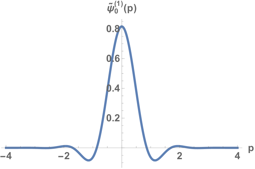
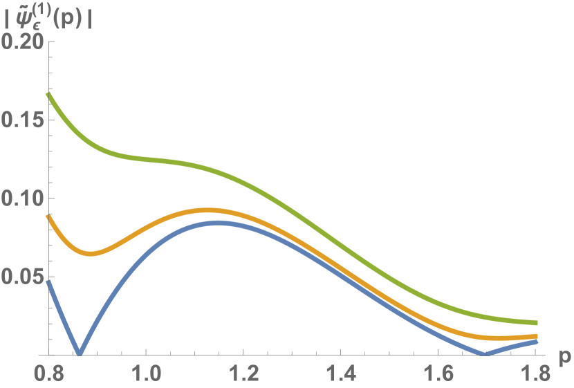
Figure 1: (left) The first function in momentum space with deformation parameter zero (right) Close up view of the magnitude of the first function for deformation parameter $\epsilon=0$ with zeros at $p_{1}^{(1)}=.86336603209$ and $p_{2}^{(1)}=1.696081937$ (blue), $\epsilon=.1$ (orange) and $\epsilon=.2$ (green) with no zeros.

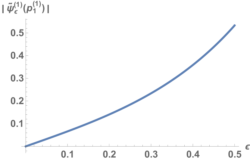
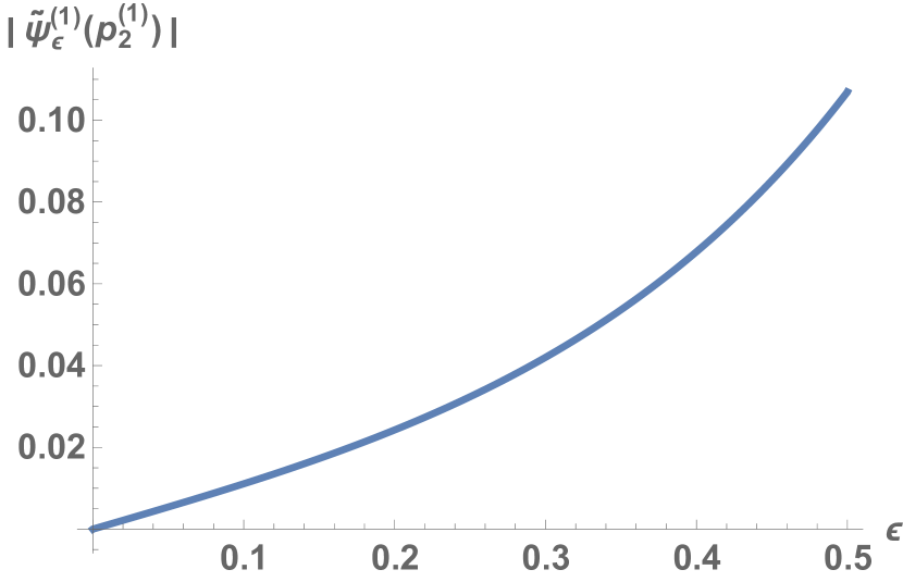
Figure 2: How the first function moves away from the (left) first zero and (right) second zero as a function of the deformation parameter $\epsilon$.

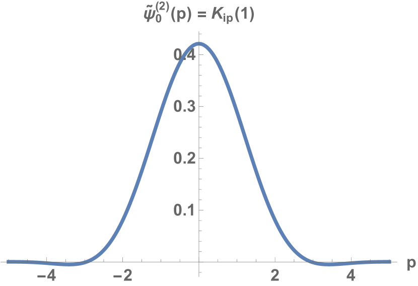
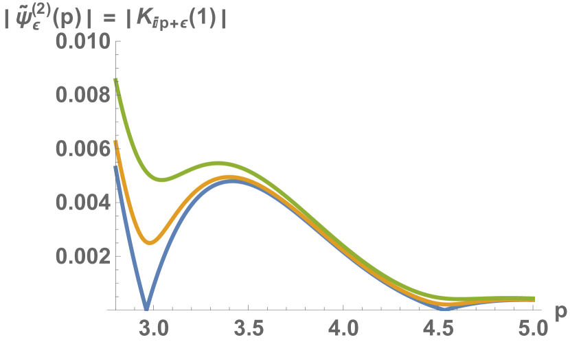
Figure 3: (left) The second function in momentum space with deformation parameter zero (right) Close up view of the magnitude of the second function for deformation parameter $\epsilon=0$ with zeros at $p_{1}^{(2)}=2.962548534571$ and $p_{2}^{(2)}=4.534490718$ (blue), $\epsilon=.1$ (orange) and $\epsilon=.2$ (green) with no zeros.

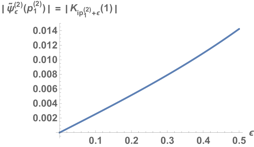
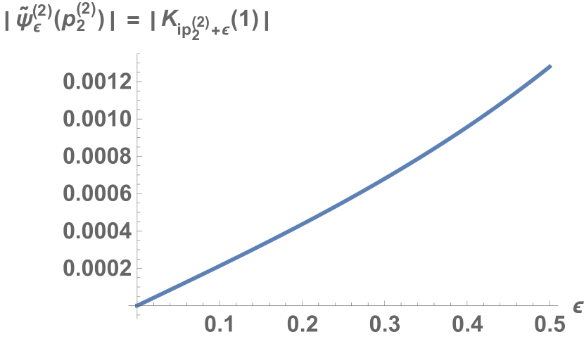
Figure 4: How the second function moves away from the (left) first zero and (right) second zero as a function of the deformation parameter $\epsilon$.

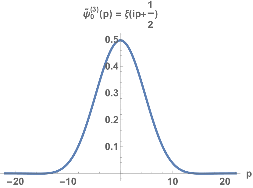
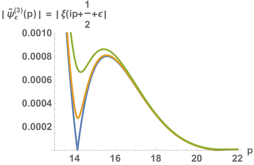
Figure 5: (left) The third function in momentum space with deformation parameter zero (right) Close up view of the magnitude of the second function for deformation parameter $\epsilon=0$ with zeros at $p_{1}^{(3)}=14.134725141734695$ and $p_{2}^{(3)}=21.022039638771556$ (blue), $\epsilon=.2$ (orange) and $\epsilon=.5$ (green) with no zeros.

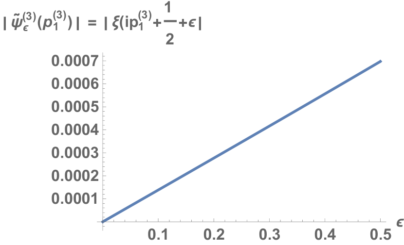
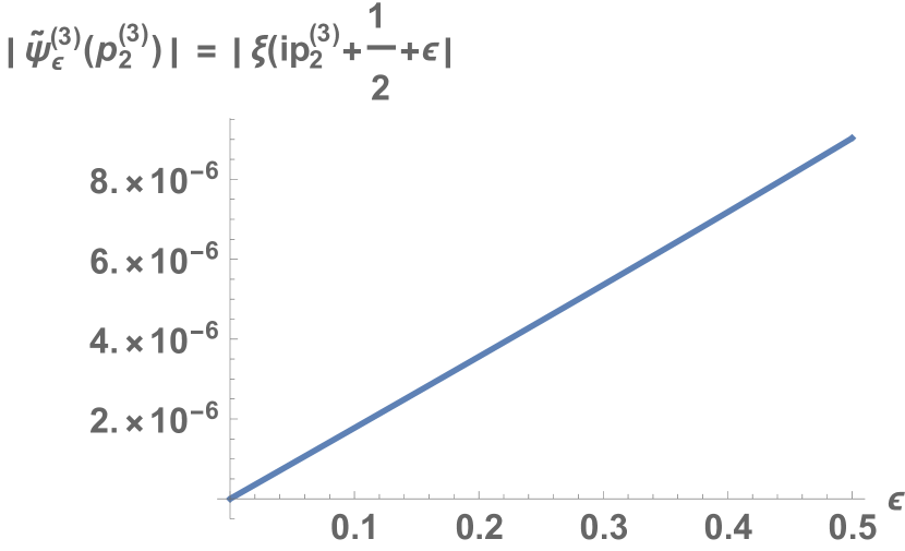
Figure 6: How the third function moves away from the (left) first zero and (right) second zero as a function of the deformation parameter $\epsilon$.

3 Quantum Fourier transform on a quantum computer

The Quantum Fourier Transform (QFT) algorithm is based on a quantum computers innate ability to represent the operation of Unitary matrices on quantum states. On a quantum computer both the Unitary matrix and the states are represented in terms of qubits which are acted on but quantum gates and represented in a quantum circuit. The Unitary matrix that the QFT algorithm represents in the Sylvester matrix $F$. In terms of quantum systems this matrix allows one to transform from a discrete version of states in position space to a discrete version of states in momentum space. In the position basis the position matrix $Q_{pos}$ is given by the diagonal matrix:

$${\left({{Q_{pos}}}\right)_{j,k}}=\sqrt{\frac{{2\pi}}{{4N}}}(2j-(N+1)){\delta_{j,k}}$$ (3.1)

and the momentum matrix $P_{pos}$ obtained from this through the operation of the Sylvester matrix by [16]:

$${P_{pos}}={F^{\dagger}}{Q_{pos}}F$$ (3.2)

where

$${F_{j,k}}=\frac{1}{{\sqrt{N}}}{e^{\frac{{2\pi i}}{{4N}}(2j-(N+1))(2k-(N+1))}}$$ (3.3)

In the same way quantum states in the position space are related to the states in momentum basis through the operation of $F$ which implements the QFT. A quantum circuit we used to apply the QFT to our functions is shown in figure 7. We used six qubits in our computations hence the six horizontal lines in the diagram. The six qubits represented 64 data points for the initial and transformed state. Also note the high depth nature of the QFT circuit as there are many gates and the circuit stretches out far in the horizontal direction. Nevertheless we were able to see the proper structure of the three functions as well as position of the first zeros. More details of the functions can emerge as more qubits and longer coherence times become feasible. The Quantum Fourier Transform is potentially exponentially faster on a fault tolerant quantum computer than the classical Fast Fourier Transform algorithm. It is one of the core quantum computing algorithms on which many important algorithms, for example Shor’s factoring algorithm, is based. The procedure we use for the QFT algorithm is to go between the position and momentum ground states associated with the three functions above and investigate the ability in determining the zeros of the functions. The QFT works by representing the Sylvester matrix as a Unitary matrix, expanding the Unitary matrix systematically in terms of gates and using these gates to form a quantum circuit. This quantum circuit is evaluated with discrete data in terms of the quantum ground state in position space with the output yielding the quantum state in momentum space, also represented in terms of discrete data and qubits. The results of the QFT are then analyzed to see if they are accurate enough to determine the zeros of the functions and how they move away from zero as one turns on the deformation parameter $\epsilon$. Our QFT simulations were done using the IBM QISkit state vector simulator. The same quantum computations can be done on near term quantum computers such as those using superconducting qubits but there is noise and errors present in the gates which cause errors in the QFT [18]. Recently however a simple type of quantum error correction has been implemented by Google [19] which may improve the accuracy running on quantum hardware in the near future. Our results are recorded in figures 8-19. We were able to use the QFT method to determine the zeros of the three functions although the results were difficult to pick out because of the small value of the functions near the zeros. In particular for the third function it was necessary to take the log of the absolute value of the data points to see the existence and location of the zeros ( see figure 18-19).

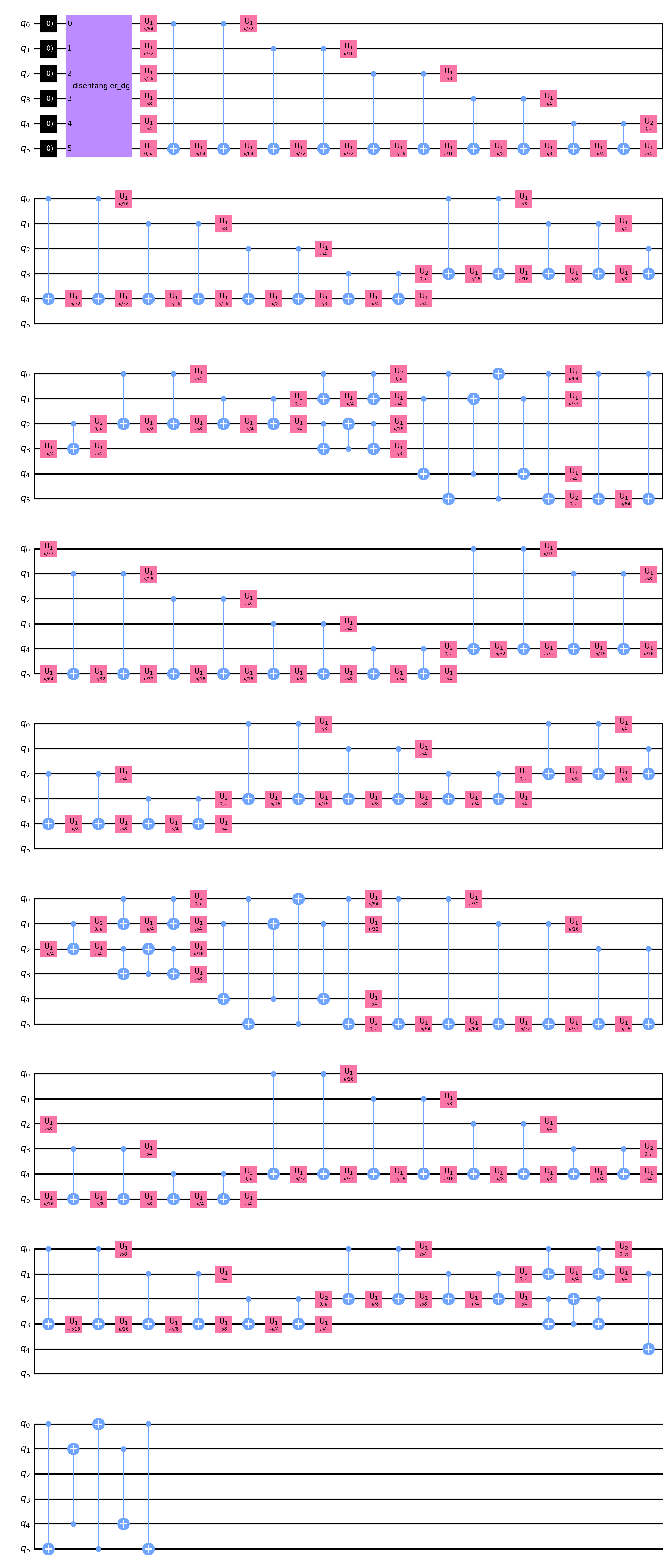
Figure 7: Quantum circuit used to implement the Quantum Fourier Transform (QFT) with six qubits using the IBM QISKit state vector simulator. Because of the length of the cirtcuit the diagram was broken in nine pieces for ease of viewing.

Figure 8: Ground state wave function (left) in position space and (right) in momentum space after Fourier transformation with deformation parameter $\epsilon=0$.

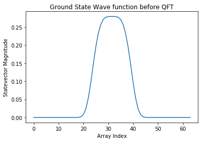
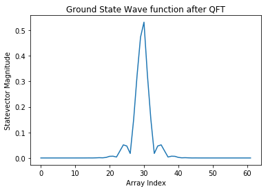
Figure 9: Magnitude of the ground state wave function (left) in position space and (right) in momentum space after Quantum Fourier transformation with deformation parameter $\epsilon=0$.

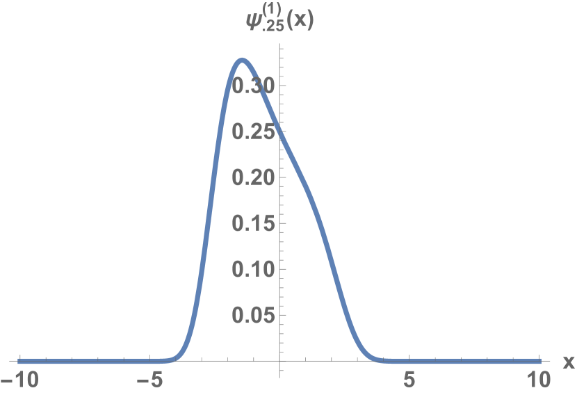
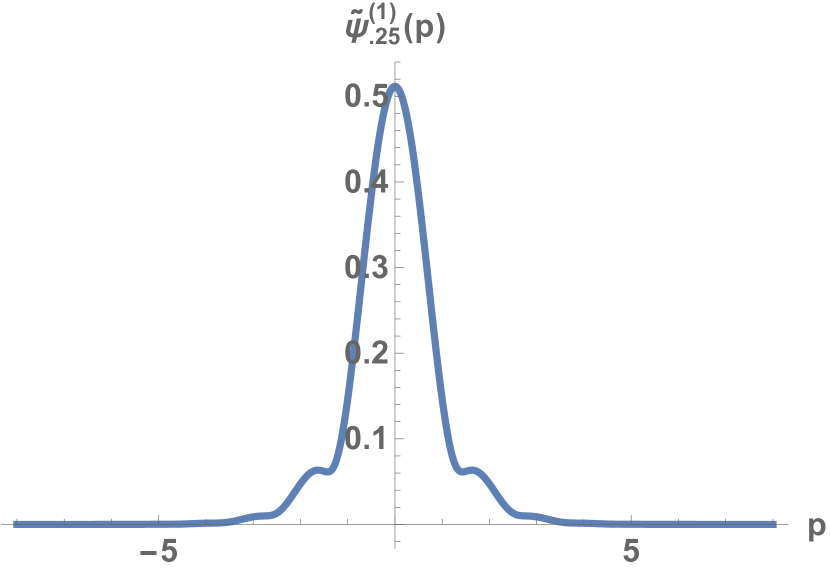
Figure 10: Magnitude of the first ground state wave function (left) in position space and (right) in momentum space after Fourier transformation with deformation parameter $\epsilon=.25$.

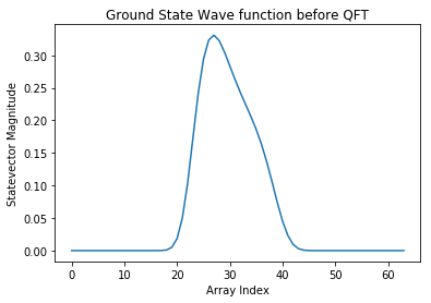
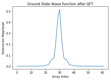
Figure 11: Magnitude of the first ground state wave function (left) in position space and (right) in momentum space after Quantum Fourier transformation with deformation parameter $\epsilon=.25$.

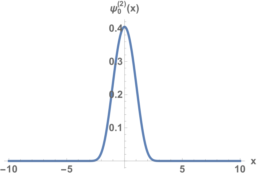
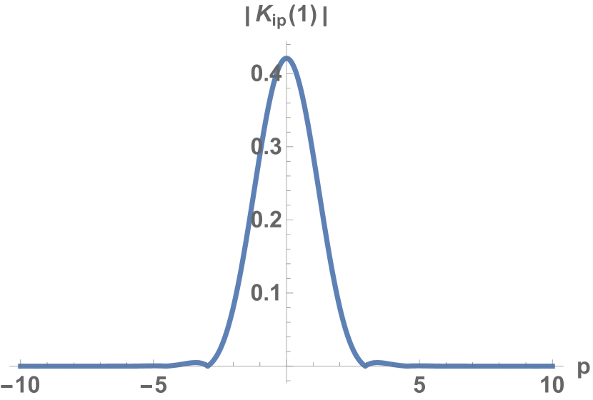
Figure 12: Magnitude of the second ground state wave function (left) in position space and (right) in momentum space after Fourier transformation with deformation parameter $\epsilon=0$.

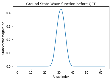
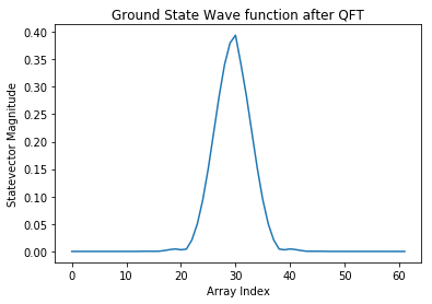
Figure 13: Magnitude of the second ground state wave function (left) in position space and (right) in momentum space after Quantum Fourier transformation with deformation parameter $\epsilon=0$.

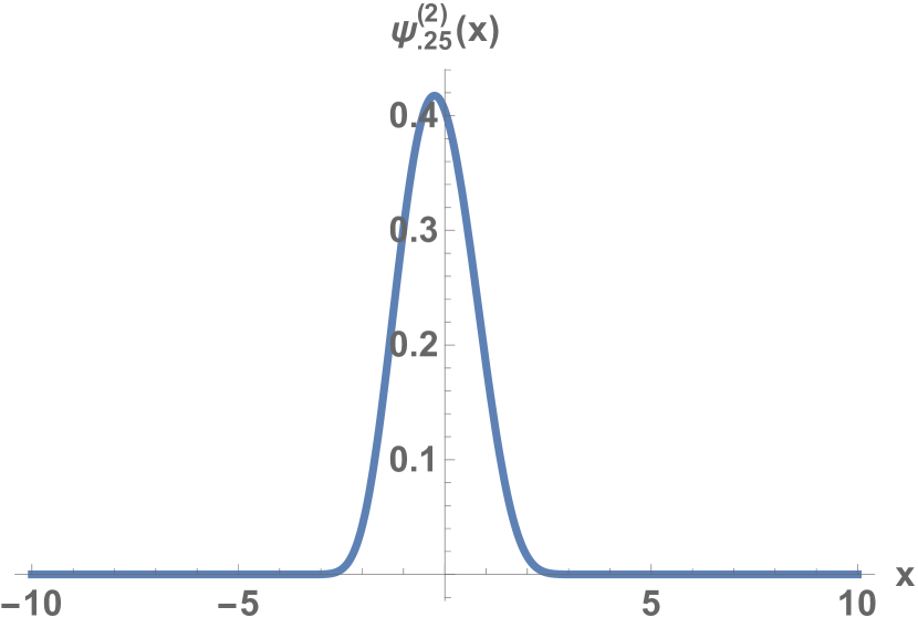
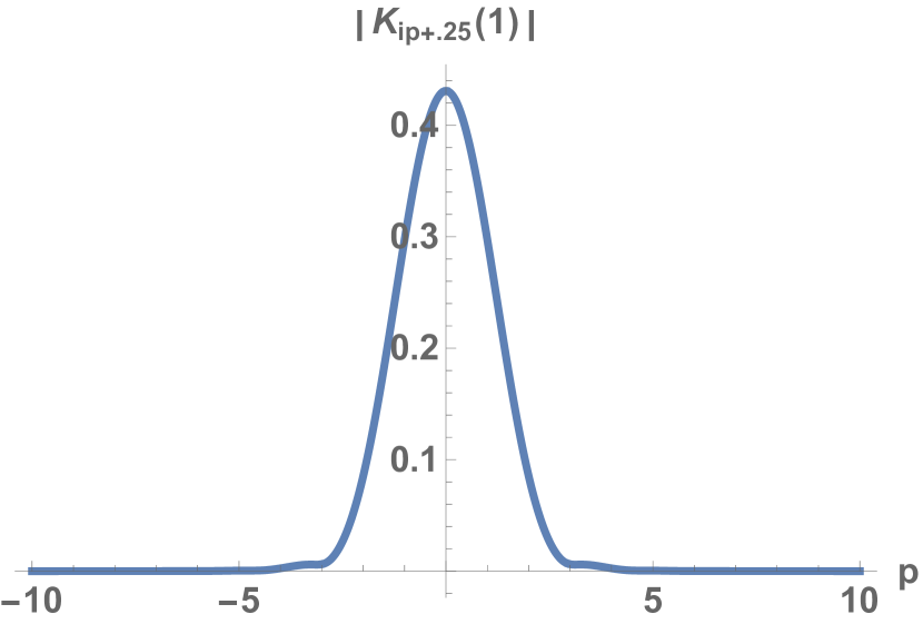
Figure 14: Magnitude of the second ground state wave function (left) in position space and (right) in momentum space after Fourier transformation with deformation parameter $\epsilon=.25$.

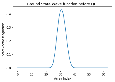
Figure 15: Magnitude of the second ground state wave function (left) in position space and (right) in momentum space after Quantum Fourier transformation with deformation parameter $\epsilon=.25$.

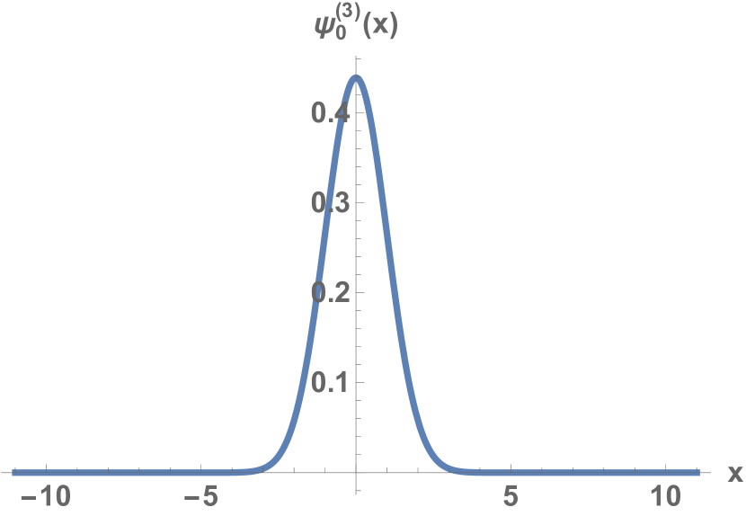
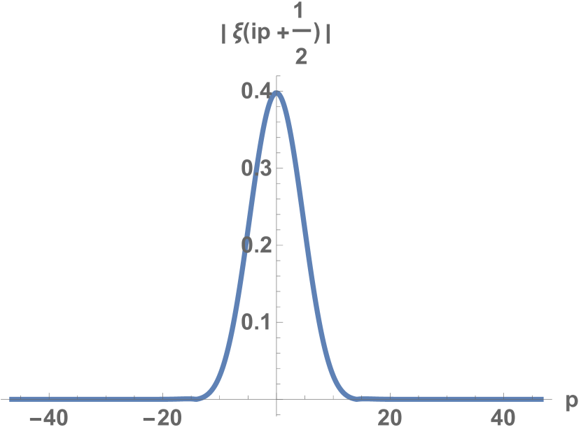
Figure 16: Magnitude of the third ground state wave function (left) in position space and (right) in momentum space after Fourier transformation with deformation parameter $\epsilon=0$.

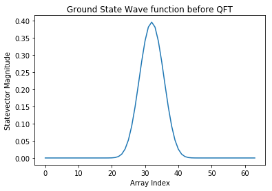
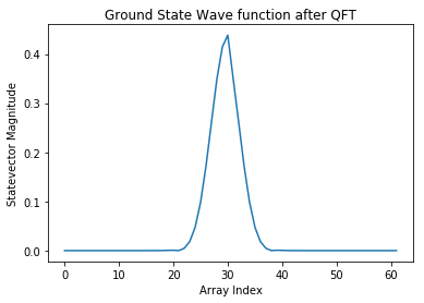
Figure 17: Magnitude of the third ground state wave function (left) in position space and (right) in momentum space after Quantum Fourier transformation with deformation parameter $\epsilon=0$.

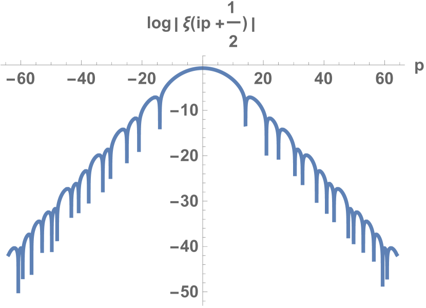
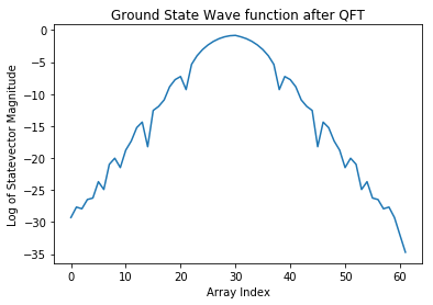
Figure 18: Log of the magnitude of the third ground state wave function in momentum space (left) using the exact expression and (right)using the Quantum Fourier transformation with deformation parameter $\epsilon=0$.

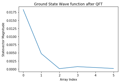
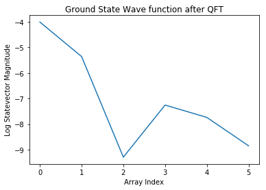
Figure 19: Zoom in on the (left) the magnitude and (right) log of the magnitude of the third ground state wave function in momentum space using the Quantum Fourier transformation with deformation parameter $\epsilon=0$.

4 Relation to supersymmetric quantum mechanics

Recently there has been several investigations of the interesting relation of supersymmetric quantum mechanics to the Riemann hypothesis [20] [21] [22] [23]. All three of the functions discussed above can be realized as ground state wave functions in supersymmetric quantum mechanics (SUSY-QM). In supersymmetric quantum mechanics the superpotential plays a key role [24]. There are two partner potentials and Hamiltonians (plus and minus) which are determined from the superpotential. The minus partner potential determines the the ground state wave function. The minus partner potential $V_{(}x)$ is determined from the superpotential $W(x)$ by:

$${V_{-}}(x)={W^{2}}(x)-W^{\prime}(x)$$ (4.1)

The ground state wave function is determined exactly in SUSYQM also from the superptential through

$$\psi(x)={e^{-\int_{0}^{x}{W(x^{\prime})dx^{\prime}}}}$$ (4.2)

The reason for this simple expression is that the Hamiltonian in SUSY-QM is expressed as the product of two operators which are first order in momentum and allows the ground state to be solved for in terms of the superpotential.

For the first function $\psi_{\epsilon}^{(1)}(x)$ the superpotential is

$${W^{(1)}}(x)=g{x^{3}}+\epsilon$$ (4.3)

with $g$ a coupling constant and the minus partner potential is given by:

$$V_{-}^{(1)}(x)={g^{2}}{x^{6}}+2\epsilon g{x^{3}}+{\epsilon^{2}}-3g{x^{2}}$$ (4.4)

finally the ground state wave function is identified with the first function:

$$\psi_{\epsilon}^{(1)}(x)={e^{-\frac{{g{x^{4}}}}{4}-\epsilon x}}$$ (4.5)

For the second function $\psi_{\epsilon}^{(2)}(x)$ the superpotential is:

$${W^{(2)}}(x)=g\sinh(x)+\epsilon$$ (4.6)

and the minus partner potential is:

$$V_{-}^{(2)}(x)={g^{2}}{\left({\sinh x}\right)^{2}}+\epsilon^{2}+2\epsilon g\sinh x-g\cosh x$$ (4.7)

and the ground state wave function is:

$$\psi_{\epsilon}^{(2)}(x)={e^{-g\cosh(x)-\epsilon x}}$$ (4.8)

Finally for the third function $\psi_{\epsilon}^{(2)}(x)$ the superpotential is

$${W^{(3)}}(x)=-\frac{{\Phi^{\prime}(x)}}{{\Phi(x)}}+\epsilon$$ (4.9)

the minus partner potential is given by

$$V_{-}^{(3)}(x)=-2\epsilon\frac{{\Phi^{\prime}(x)}}{{\Phi(x)}}+{\epsilon^{2}}+\frac{{\Phi^{\prime\prime}(x)}}{{\Phi(x)}}$$ (4.10)

and the ground state wave function is:

$$\psi_{\epsilon}^{(2)}(x)=\Phi(x){e^{-\epsilon x}}$$ (4.11)

The potentials and ground state ground state wave functions in position space are plotted in figures 20-22. The parameter $\epsilon$ doesn’t break supersymmetry but causes the potential and ground state wave function to break parity invariance $x\rightarrow-x$. The parameter $\epsilon$ affects the existence of zeros in momentum space and the Riemann hypothesis is equivalent to the statement that there are no zeros if the parameter $\epsilon$ is nonzero. Supersymmetric quantum mechanics can be realized on quantum computers where the Hamiltonian and quantum states are realized in terms of qubits [25] [26] [27] [28] [29] [30]. The ground state wave function can be determined from the Variation Quantum Eigensolver (VQE) or Quantum Phase Estimation (QPE) which can be used in conjunction with the QFT algorithm to determine the zeros associated with the three functions above. The identification of the three functions as the ground state of the Hamiltonian has some advantages in understanding the properties of the function. For example ground state wave functions do not have nodes or zeros in position space but may or may not have them in momentum space. Also the ground state wave function may or may not be symmetric in position space but the wave function is always symmetric in momentum space.

In supersymmetric quantum mechanics one defined an operator $A$ given by:

$$A=ip+W(x)$$ (4.12)

such that

$$A\psi_{\varepsilon}^{(i)}=0$$ (4.13)

For the first function with $\epsilon=0$ this operator is

$$A=ip+g{x^{3}}$$ (4.14)

so that in position space using $p=-i\frac{\partial}{{\partial x}}$ this becomes:

$$\left({\frac{\partial}{{\partial x}}+g{x^{3}}}\right)\psi_{0}^{(1)}(x)=0$$ (4.15)

In momentum space using $x=i\frac{\partial}{{\partial p}}$ we have:

$$\left({ip-ig\frac{{{\partial^{3}}}}{{\partial{p^{3}}}}}\right)\tilde{\psi}_{0}^{(1)}(p)=0$$ (4.16)

or equivalently

$$\left({-\frac{{{\partial^{3}}}}{{\partial{p^{3}}}}+\frac{1}{g}p}\right)\tilde{\psi}_{0}^{(1)}(p)=0$$ (4.17)

For $g=\frac{1}{64}$ we have for the generalized Airy function

$$\left({-\frac{{{\partial^{3}}}}{{\partial{p^{3}}}}+64p}\right)A{i_{3}}(p)=0$$ (4.18)

an equation we shall see in the next section related to the $(3,1)$ Random two Matrix model.

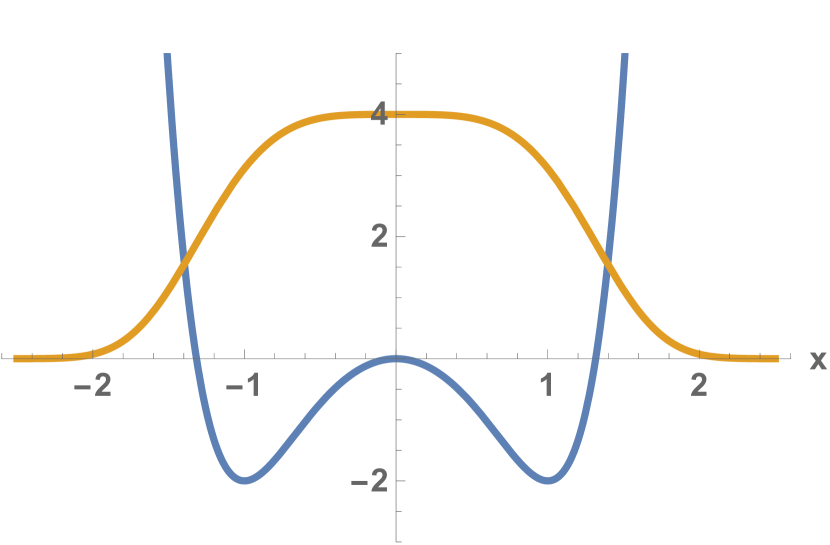
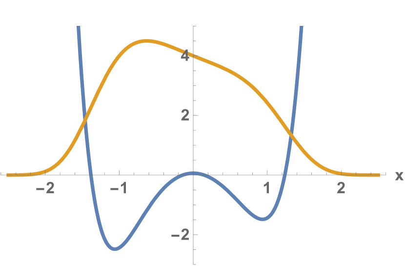
Figure 20: Minus partner potential (blue) and first ground state wave function (orange) for deformation parameter $\epsilon=0$ (left) and $\epsilon=.25$ (right).

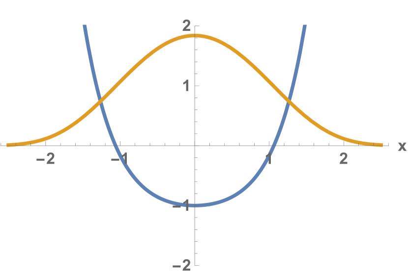
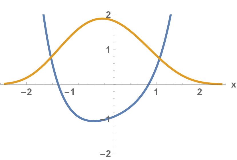
Figure 21: Minus partner potential (blue) and second ground state wave function (orange) for deformation parameter $\epsilon=0$ (left) and $\epsilon=.25$ (right).

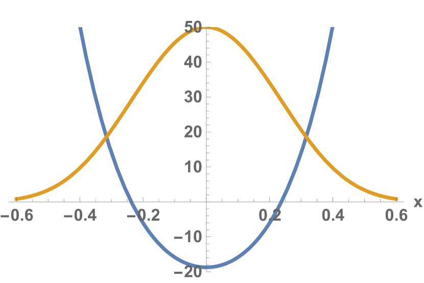
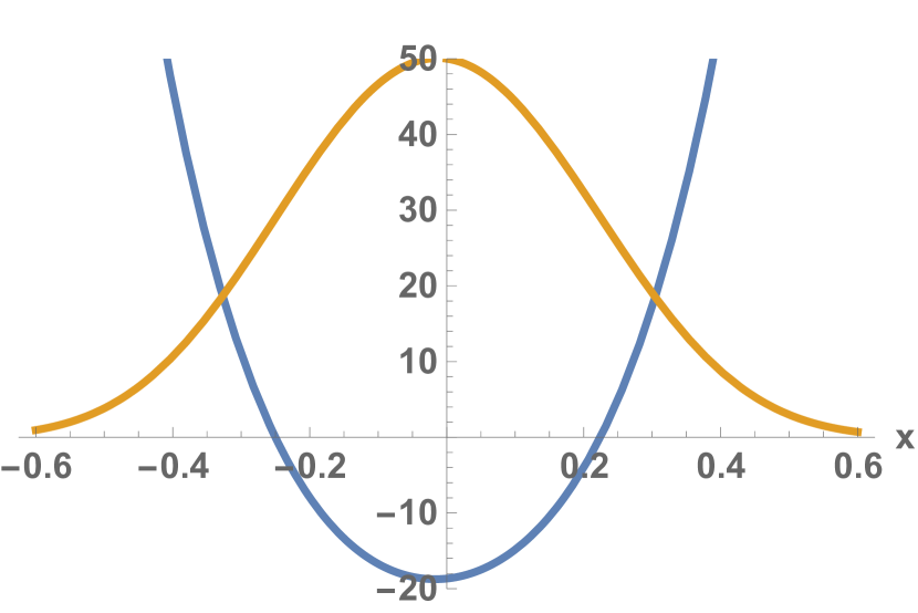
Figure 22: Minus partner potential (blue) and third ground state wave function (orange) for deformation parameter $\epsilon=0$ (left) and $\epsilon=.25$ (right).

5 Relation to Random Matrix Theory

Random matrix theory has interesting connections to the Riemann zeta function [31][32] [33]. For example the spacing of zeros on the critical line correspond to pair correlations of eigenvalues in a Gaussian Unitary Ensemble (GUE). In this section we study a connection of the type of functions in this paper to the scaling limit of a $(p,1)$ minimal Matrix model [34] [35] [36] [37] [38] [39] [40] [41] [42] where $p$ is an integer describing the order of the Matrix potential (not to be confused with $p$ used for momentum space above). The case we will study the first function is the (3,1) Minimal Matrix model but the other two functions can be considered using higher values of $p$ and deformations of the potential of the matrix model. The quantity of interest in relation to the zeros of the three functions is the expectation value of the characteristic potential of a hermitian matrix in the ensemble which is represented by a matrix integral as:

$$\left\langle{\det(y-B)}\right\rangle={Z_{p,1}}{(g)^{-1}}\int{dAdB{e^{-\frac{1}{g}Tr({V_{p}}(A+1)-AB)}}\det(y-B)}$$ (5.1)

where $g$ is the coupling constant of the matrix model, $N\times N$ is the size of the Hermitian Matrices $A$ and $B$ where

$${Z_{p,1}}(g)={\left({2\pi g}\right)^{{N^{2}}}}$$ (5.2)

and the matrix potential is

$${V_{p}}(a)=-\sum\limits_{k=1}^{p}{\left({\frac{{{a^{k}}}}{k}-\frac{1}{k}}\right)}$$ (5.3)

or alternatively

$${V_{p}}(a)=-\int_{1}^{a}{\sum\limits_{k=0}^{p-1}{a{{}^{\prime k}}}da^{\prime}}$$ (5.4)

The matrix model can be solved using orthogonal polynomials with orthonormal relations

$$\int{dadb{e^{-\frac{1}{g}({U_{p}}(a+1)-ab)}}{P_{m}}(a){Q_{n}}(b)={h_{m}}{\delta_{mn}}}$$ (5.5)

with $h_{m}$ a sequence that can be determined order by order. The solution yields the closed expression for the expectation value of the characteristic polynomial in terms of the $N$th orthogal polynomial.

$$\left\langle{\det(y-B)}\right\rangle={Q_{N}}(y)={\left({-g\frac{\partial}{{\partial z}}}\right)^{N}}{\left.{{e^{\frac{1}{g}\left({{U_{p}}(z+1)-yz}\right)}}}\right|_{z=0}}$$ (5.6)

To see the relation to our first function we specialize to the case $p=3$ so that:

$${V_{3}}(a+1)=-\frac{{{a^{3}}}}{3}-\frac{{3{a^{2}}}}{2}-3a$$ (5.7)

It is interesting that for large $N$ the zeros of the polynomials $Q_{N}(y)$ are real. We plot the zeros for $N=200$ and $N=400$ in figures 23. The relation to the generalized Airy function occurs through the scaling limit where one has:

$$g=\frac{1}{N}$$ (5.8)

and

$$y={\left({\frac{1}{N}}\right)^{\frac{p}{{p+1}}}}\tilde{y}={N^{-3/4}}\tilde{y}$$ (5.9)

the generalized Airy function is given by:

$$\psi({N^{3/4}}y)=\frac{1}{{\sqrt{2\pi N}}}{N^{1/4}}{e^{N}}{e^{-yN}}{Q_{N}}(y)$$ (5.10)

$$\psi(\tilde{y})=\frac{1}{{\sqrt{2\pi N}}}{N^{1/4}}{e^{N}}{e^{-\tilde{y}{N^{1/4}}}}{Q_{N}}({N^{-3/4}}\tilde{y})=\frac{1}{{\sqrt{2\pi N}}}{N^{1/4}}{e^{N}}{e^{-\tilde{y}{N^{1/4}}}}\left\langle{\det({N^{-3/4}}\tilde{y}-B)}\right\rangle$$

For large $N$ the expectation value of the characteristic polynomial is the characteristic polynomial of a particular matrix called the master matrix [43] [44] [45] [46] $B_{master}$ so that

$$\left\langle{\det(y-B)}\right\rangle=\det(y-{B_{master}^{(3,1)}})$$ (5.11)

If the master matrix is Hermitian then it’s eigenvalues are real and its characteristic polynomial will have real zeros. For the $(2,1)$ matrix model the master matrix is known and is Hermitian. It is given by:

$$B_{master}^{(2,1)}=\frac{1}{{\sqrt{2}}}\left({\begin{array}[]{*{20}{c}}0&{\sqrt{1}}&0&\ldots\\ {\sqrt{1}}&0&{\sqrt{2}}&0\\ 0&{\sqrt{2}}&0&\ddots\\ \vdots&\ddots&\ddots&\ddots\end{array}}\right)$$ (5.12)

For the $(p,1)$ matrix model the master matrix is unknown and it is not clear that if it exists it will be Hermitian and an element of the matrix ensemble or a matrix outside it. The answer depends on the infinite $N$ limit used to obtain the infinite dimensional master matrix. The Riemann hypothesis is equivalent to the statement that the master matrix exists and is Hermitian so that $\psi$ can be identified as it’s characteristic polynomial. It is interesting that the Hermitian matrix $B_{master}$ of the Hilbert-Polya conjecture is not interpreted as a Hamiltonian but rather a special element of a matrix ensemble where expectation values are represented by evaluation with the master matrix. The expectation value of the characteristic polynomial is represented in the matrix model from the integration of fermions. In string field theory one can also obtain the the expectation value of the inverse of the characteristic polynomial through the integration of bosons [47]:

$$\left\langle{\frac{1}{{\det(y-B)}}}\right\rangle=\frac{1}{{\det(y-{B_{master}})}}$$ (5.13)

In this case the Riemann zeros become poles and further insight may come from the interpretation in terms of scattering amplitudes of quantum fields or string theory [48] [49]. The advantage of applying quantum computing to the Random matrix model [50] [51] [52] [53] is that a fault tolerant quantum computer with a large number of qubits can examine much larger values of $N$ than a classical computer and may yield information on the large $N$ limit and the scaling behavior of the expectation value of the characteristic polynomial.

In the $(3,1)$ random two Matrix model the function $\psi(y)$ obeys the third order differential equation [34]

$$\frac{{{\partial^{3}}}}{{\partial{y^{3}}}}\psi(y)=64y\psi(y)$$ (5.14)

which we identify as the equation from the previous section on supersymmetric quantum mechanics. If we denote $y_{n}$ as the nth zero of $\psi(y)$ we can write this equation as

$$\frac{{{\partial^{3}}}}{{\partial{y^{3}}}}\psi(y-{y_{n}})=64\left({y-{y_{n}}}\right)\psi(y-{y_{n}})$$ (5.15)

or

$$-\frac{{{\partial^{3}}}}{{\partial{y^{3}}}}\psi(y-{y_{n}})+64y\psi(y-{y_{n}})=64{y_{n}}\psi(y-{y_{n}})$$ (5.16)

which we recognize as an eigenproblem for a linear potential [54] [55] with a cubic kinetic term. Returning to the momentum space representation from the previous section we write the equation as:

$$-\frac{1}{{64}}\frac{{{\partial^{3}}}}{{\partial{p^{3}}}}\psi_{0}^{(1)}(p-{p_{n}})+p\psi_{0}^{(1)}(p-{p_{n}})={p_{n}}\psi_{0}^{(1)}(p-{p_{n}})$$ (5.17)

We plot the first seven eigenfunctions of the eigenproblem whose eigenvalues are the first seven zeros of the generalized Airy function in figure 24. Finally we note that result we obtain for the zeros from the semiclassical phase integral for the linear potential eigensystem ${\left({\frac{1}{4}\left({\frac{4}{3}}\right)\left({n+\frac{3}{4}}\right)\pi}\right)^{3/4}}$ is not as accurate for the generalized Airy function as in the usual Airy function for ${\left({\left({\frac{3}{2}}\right)\left({n+\frac{3}{4}}\right)\pi}\right)^{2/3}}$ so it is important in the (3,1) Matrix model case or in the SUSY-QM treatment to use the exact expression instead of a semi-classical form.

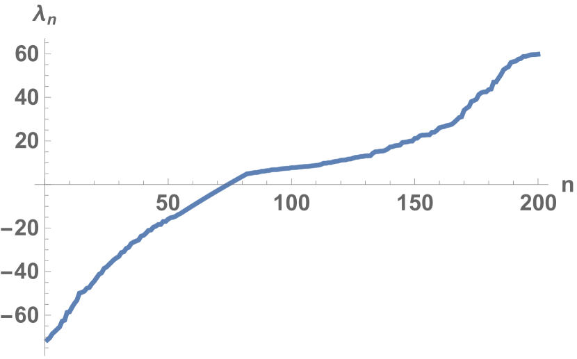
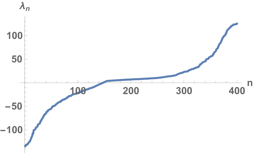
Figure 23: Zeros of the expectation value of the characteristic polynomial for the $(3,1)$ Matrix model for (left) $N=200$ and (right) $N=400$, ordered from most negative to most positive. Surprisingly these are all real..

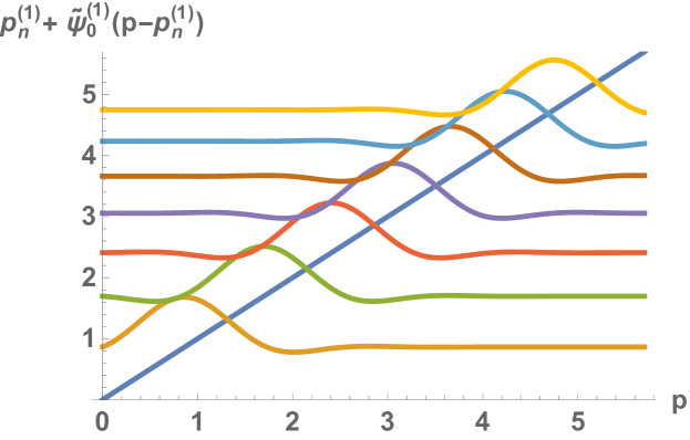
Figure 24: Solutions to the generalized Airy equation for the $(3,1)$ two matrix model and SUSY-QM with cubic superpotential transformed to momentum space and interpreted as a generalized linear potential eigensystem.

6 Conclusion

In this paper we examined the application of quantum computing to three functions with nontrivial zeros including the Riemann xi function. We found that the quantum Fourier transform algorithm can detect zeros of the three functions using a quantum circuit and supersymmetric quantum mechanics can give a representation of the functions as a ground state of a supersymmetric quantum mechanics Hamiltonian whose spectrum can be studied on a quantum computer. Finally the representation of these functions in terms of the $(p,1)$ matrix model was studied and quantum computing can be used to examine very large matrices which can approximate the master matrix of these matrix models for large values of $N$. The intersection of quantum computing, the Riemann hypothesis, supersymmetric quantum mechanics and matrix models is an exciting area of future research to explore.

References

- [1] W. van Dam, “Quantum Computing and Zeroes of Zeta Functions”, ¡i¿arXiv e-prints¡/i¿, 2004. doi:10.48550/arXiv.quant-ph/0405081.
- [2] J. I. Latorre and G. Sierra, “Quantum Computation of Prime Number Functions,” Quant. Inf. Comput. 14, 577-588 (2014) [arXiv:1302.6245 [quant-ph]].
- [3] G. Sierra, “The Riemann zeros as spectrum and the Riemann hypothesis,” Symmetry 11, no.4, 494 (2019) doi:10.3390/sym11040494 [arXiv:1601.01797 [math-ph]].
- [4] G. Sierra, “The Riemann zeros as energy levels of a Dirac fermion in a potential built from the prime numbers in Rindler spacetime,” J. Phys. A 47, no.32, 325204 (2014) doi:10.1088/1751-8113/47/32/325204 [arXiv:1404.4252 [math-ph]].
- [5] Finding zeros of the Riemann zeta function by periodic driving of cold atoms C. E. Creffield and G. Sierra Phys. Rev. A 91, 063608 – Published 8 June 2015
- [6] R. He, R. et al, “Riemann zeros from a periodically-driven trapped ion”, 2021. doi:10.48550/arXiv.2102.06936.
- [7] ”Identifying the Riemann zeros by periodically driving a single qubit” Ran He, Ming-Zhong Ai, Jin-Ming Cui, Yun-Feng Huang, Yong-Jian Han, Chuan-Feng Li, Tao Tu, C. E. Creffield, G. Sierra, and Guang-Can Guo Phys. Rev. A 101, 043402 – Published 9 April 2020
- [8] R. He et al ”Riemann zeros from Floquet engineering a trapped-ion qubit.”, npj Quantum Information 7. doi:10.1038/s41534-021-00446-7
- [9] https://gilkalai.wordpress.com/about/pages/conversation-with-the-ai-program-gpt3/
- [10] https://terrytao.wordpress.com/2014/12/15/254a-supplement-3-the-gamma-function-and-the-functional-equation-optional/
- [11] J. L. Lopez, J. L. and P. J. Pagola, “Analytic formulas for the evaluation of the Pearcey integral”, 2016. doi:10.48550/arXiv.1601.03615.
- [12] E. Espíndola-Ramos, “Classical characterization of quantum waves: comparison between the caustic and the zeros of the Madelung–Bohm potential”, Journal of the Optical Society of America A, vol. 38, no. 3, p. 303, 2021. doi:10.1364/JOSAA.411094.
- [13] Lopez, J. L. and Pagola, P., “The Pearcey integral in the highly oscillatory region”, 2015. doi:10.48550/arXiv.1511.05323.
- [14] L. Fidkowski, V. Hubeny, M. Kleban and S. Shenker, “The Black hole singularity in AdS / CFT,” JHEP 02, 014 (2004) doi:10.1088/1126-6708/2004/02/014 [arXiv:hep-th/0306170 [hep-th]].
-
[15]
B. Rogers, T. Tao,
”The De Bruijn-Newman constant is non-negative”,
arXiv:1801.05914 [math.NT] - [16] S. Zhang and A. Vourdas, “Analytic representation of finite quantum systems,” J. Phys. A 37, 8349-8363 (2004) doi:10.1088/0305-4470/37/34/011 [arXiv:quant-ph/0504014 [quant-ph]].
- [17] L. Susskind and A. Friedman, “Quantum Mechanics: The Theoretical Minimum,” Basic Books, 2014,
- [18] D. García-Martín and G. Sierra, “Five Experimental Tests on the 5-Qubit IBM Quantum Computer”, 2017. doi:10.48550/arXiv.1712.05642.
- [19] R. Acharya et al. (Google Quantum AI), “Suppressing quantum errors by scaling a surface code logical qubit,” Nature 614, no.7949, 676-681 (2023) doi:10.1038/s41586-022-05434-1 [arXiv:2207.06431 [quant-ph]].
- [20] A. Das and P. Kalauni, “Supersymmetry and the Riemann zeros on the critical line,” Phys. Lett. B 791, 265-269 (2019) doi:10.1016/j.physletb.2019.02.040 [arXiv:1810.02204 [math.GM]].
- [21] P. Kalauni and K. A. Milton, “Supersymmetric quantum mechanics and the Riemann hypothesis,” [arXiv:2211.04382 [hep-th]].
- [22] J. D. García-Muñoz, A. Raya and Y. Concha-S, “Second-Order SUSY-QM and zeroes of the Riemann zeta function,” [arXiv:2301.05360 [math-ph]].
- [23] M. McGuigan, “Riemann Hypothesis, Modified Morse Potential and Supersymmetric Quantum Mechanics,” [arXiv:2002.12825 [math-ph]].
- [24] A. Gangopadhyaya, J. V. Mallow and C. Rasinariu, “Supersymmetric Quantum Mechanics: An Introduction,” World Scientific, 2017, ISBN 978-981-4313-08-7, 978-981-322-103-1, 978-981-322-104-8 doi:10.1142/10475
- [25] C. Kane and M. McGuigan, ”Visualizing effective potentials and using the IBM-Q to study quantum field theory models in 0+1 dimensions”, New York Scientific Data Summit (NYSDS), pp. 16, Aug 2018.
- [26] R. Miceli, and M. McGuigan, “Quantum Computation and Visualization of Hamiltonians using Discrete Quantum Mechanics and IBM QISKit”, New York Scientific Data Summit (NYSDS), Aug 2018, doi:10.48550 [arXiv:1812.01044 [quant-ph]].
- [27] J. Apanavicius, Y. Feng, Y. Flores, M. Hassan and M. McGuigan, “Morse Potential on a Quantum Computer for Molecules and Supersymmetric Quantum Mechanics,” [arXiv:2102.05102 [quant-ph]].
- [28] Y. Feng, M. McGuigan and T. White, “Superconformal Quantum Mechanics on a Quantum Computer,” [arXiv:2201.00805 [quant-ph]].
- [29] C. Culver and D. Schaich, “Quantum Computing for the Wess–Zumino Model,” PoS LATTICE2022, 008 (2023) doi:10.22323/1.430.0008 [arXiv:2301.02230 [hep-lat]].
- [30] C. Culver and D. Schaich, “Quantum computing for lattice supersymmetry,” PoS LATTICE2021, 153 (2022) doi:10.22323/1.396.0153 [arXiv:2112.07651 [hep-lat]].
- [31] A.J.Izenman, ”Introduction to Random Matrix Theory and it’s Applications”, Statist. Sci. 36 (3) 421 - 442, August 2021. https://doi.org/10.1214/20-STS799
- [32] C. A. Tracy and H. Widom, “Introduction to random matrices,” Lect. Notes Phys. 424, 103 (1993) doi:10.1007/BFb0021444 [arXiv:hep-th/9210073 [hep-th]].
- [33] D. Anninos and B. Mühlmann, “Notes on matrix models (matrix musings),” J. Stat. Mech. 2008, 083109 (2020) doi:10.1088/1742-5468/aba499 [arXiv:2004.01171 [hep-th]].
- [34] A. Hashimoto, M. x. Huang, A. Klemm and D. Shih, “Open/closed string duality for topological gravity with matter,” JHEP 05, 007 (2005) doi:10.1088/1126-6708/2005/05/007 [arXiv:hep-th/0501141 [hep-th]].
- [35] R. Gopakumar and E. A. Mazenc, “Deriving the Simplest Gauge-String Duality - I: Open-Closed-Open Triality,” [arXiv:2212.05999 [hep-th]].
- [36] D. Gaiotto and L. Rastelli, “A Paradigm of open / closed duality: Liouville D-branes and the Kontsevich model,” JHEP 07, 053 (2005) doi:10.1088/1126-6708/2005/07/053 [arXiv:hep-th/0312196 [hep-th]].
- [37] M. Bertola, B. Eynard and J. P. Harnad, “Duality, biorthogonal polynomials and multimatrix models,” Commun. Math. Phys. 229, 73-120 (2002) doi:10.1007/s002200200663 [arXiv:nlin/0108049 [nlin.SI]].
- [38] S. K. Ashok and J. Troost, “Topological Open/Closed String Dualities: Matrix Models and Wave Functions,” JHEP 09, 064 (2019) doi:10.1007/JHEP09(2019)064 [arXiv:1907.02410 [hep-th]].
- [39] N. Seiberg and D. Shih, “Flux vacua and branes of the minimal superstring,” JHEP 01, 055 (2005) doi:10.1088/1126-6708/2005/01/055 [arXiv:hep-th/0412315 [hep-th]].
- [40] N. Seiberg and D. Shih, “Minimal string theory,” Comptes Rendus Physique 6, 165-174 (2005) doi:10.1016/j.crhy.2004.12.007 [arXiv:hep-th/0409306 [hep-th]].
- [41] J. M. Maldacena, G. W. Moore, N. Seiberg and D. Shih, “Exact vs. semiclassical target space of the minimal string,” JHEP 10, 020 (2004) doi:10.1088/1126-6708/2004/10/020 [arXiv:hep-th/0408039 [hep-th]].
- [42] P. Bleher and A. Its, “Double scaling limit in the random matrix model: The Riemann-Hilbert approach,” [arXiv:math-ph/0201003 [math-ph]].
- [43] F. R. Klinkhamer, “IIB matrix model, bosonic master field, and emergent spacetime,” PoS CORFU2021, 259 (2022) doi:10.22323/1.406.0259 [arXiv:2203.15779 [hep-th]].
- [44] R. Gopakumar and D. J. Gross, “Mastering the master field,” Nucl. Phys. B 451, 379-415 (1995) doi:10.1016/0550-3213(95)00340-X [arXiv:hep-th/9411021 [hep-th]].
- [45] E. Witten, The 1/N expansion in atomic and particle physics, in: G. ’t Hooft et. al (eds.), Recent Developments in Gauge Theories, Plenum Press, New York, USA, 1980, pp. 403–419
- [46] S. Coleman, 1/N, in: Aspects of Symmetry: Selected Erice Lectures, Cambridge University Press, Cambridge, UK, 1985, pp. 351–402
- [47] S. Zeze, “A Matrix model from string field theory,” Front. in Phys. 4, 39 (2016) doi:10.3389/fphy.2016.00039 [arXiv:1507.03164 [hep-th]].
- [48] G. N. Remmen, “Amplitudes and the Riemann Zeta Function,” Phys. Rev. Lett. 127, no.24, 241602 (2021) doi:10.1103/PhysRevLett.127.241602 [arXiv:2108.07820 [hep-th]].
- [49] N. N. Khuri, “Inverse scattering, the coupling constant spectrum, and the Riemann hypothesis,” Math. Phys. Anal. Geom. 5, 1-63 (2002) doi:10.1023/A:1015813727650 [arXiv:hep-th/0111067 [hep-th]].
- [50] R. Miceli and M. McGuigan, “Effective matrix model for nuclear physics on a quantum computer,” doi:10.1109/NYSDS.2019.8909693
- [51] E. Rinaldi, X. Han, M. Hassan, Y. Feng, F. Nori, M. McGuigan and M. Hanada, “Matrix-Model Simulations Using Quantum Computing, Deep Learning, and Lattice Monte Carlo,” PRX Quantum 3, no.1, 010324 (2022) doi:10.1103/PRXQuantum.3.010324 [arXiv:2108.02942 [quant-ph]].
- [52] V. Chandra, Y. Feng and M. McGuigan, “A Matrix Big Bang on a Quantum Computer,” [arXiv:2212.00260 [quant-ph]].
- [53] N. Butt, P. Draper and J. Shen, “Simulating the Femtouniverse on a Quantum Computer,” [arXiv:2211.10870 [hep-lat]].
- [54] J. Gea-Banacloche, (1999). A quantum bouncing ball. American Journal of Physics - AMER J PHYS. 67. 776-782. 10.1119/1.19124.
- [55] J. A. Anaya-Contreras, A. Zúñiga-Segundo and H. M. Moya-Cessa, “Airy eigenstates and their relation to coordinate eigenstates,” Results Phys. 31, 104904 (2021) doi:10.1016/j.rinp.2021.104904 [arXiv:2012.15689 [quant-ph]].