FCN+$\colon$ Global Receptive Convolution Makes FCN Great Again

Abstract

Fully convolutional network (FCN) is a seminal work for semantic segmentation. However, due to its limited receptive field, FCN cannot effectively capture global context information which is vital for semantic segmentation. As a result, it is beaten by state-of-the-art methods which leverage different filter sizes for larger receptive fields. However, such a strategy usually introduces more parameters and increases the computational cost. In this paper, we propose a novel global receptive convolution (GRC) to effectively increase the receptive field of FCN for context information extraction, which results in an improved FCN termed FCN+. The GRC provides global receptive field for convolution without introducing any extra learnable parameters. The motivation of GRC is that different channels of a convolutional filter can have different grid sampling locations across the whole input feature map. Specifically, the GRC first divides the channels of the filter into two groups. The grid sampling locations of the first group are shifted to different spatial coordinates across the whole feature map, according to their channel indexes. This can help the convolutional filter capture the global context information. The grid sampling location of the second group remains unchanged to keep the original location information. Convolving using these two groups, the GRC can integrate the global context into the original location information of each pixel for better dense prediction results. With the GRC built in, FCN+ can achieve comparable performance to state-of-the-art methods for semantic segmentation tasks, as verified on PASCAL VOC 2012, Cityscapes and ADE20K.

1 Introduction

Semantic segmentation is a dense prediction task which aims to assign each pixel a class label. It is a fundamental yet challenging task in computer vision, with a variety of applications in scene understanding  [33, 34], autonomous vehicles [29, 25] and medical image diagnostics [23, 37]. The challenges mainly lie in the large-scale variation of objects and stuff, as well as the similar appearance of different objects. Concretely, the challenge one is that: extremely large-scale objects may cause inconsistent segmentation results on the same object while extremely small-scale objects can be easily neglected. To alleviate this issue, multi-scale feature representations are heavily used to capture objects of different scales. The challenge two: similar visual appearance of different objects probably leads to confusion on their boundaries. To better segment these boundaries, it is necessary to integrate global context information to each pixel’s representation so that overall scene understanding can be employed for correctly classifying each pixel on the boundaries.

Fully convolutional network (FCN) [20] is a seminal work for semantic segmentation tasks. It leverages deep convolutional neural networks (CNNs) to extract features for objects and scenes, and further aggregates feature maps of different spatial resolutions from hierarchical layers as multi-scale representations. Owing to this, FCN is robust to objects’ scale variation to a certain extent. However, due to its limited receptive field, FCN can hardly capture global context information.

Some other methods try to address these challenges by introducing multiple pooling layers of different pooling grids, or convolutions of different dilation rates or different grid sampling locations [33, 4, 5, 6, 7, 10]. Nevertheless, pooling layers can lose finer spatial information [33], leading to poor representations for some pixels; large dilation rates may cause gridding artifacts [5, 6] and lose neighbor information; learning grid sampling locations increases the model parameters [10] and the learned locations can be inexact. More importantly, all of these methods assume that different channels of a filter share exactly the same grid sampling locations which are limited to fixed local spatial coordinates, such as the 3$\times$3 convolutions in Figure 1(a) and (b). In an extreme case, the grid sampling location of a 1$\times$1 dilated/deformable convolution is a fixed spatial point at the feature map—no matter how many channels are involved. This is infeasible because it can never enlarge the receptive field of 1$\times$1 convolution. All these limitations may hinder their efficacy or efficiency for integrating global context information to pixel-wise representations.

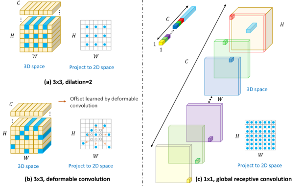
Figure 1: Comparison of global receptive convolution with the other convolutions. (a) 3$\times$3 dilated convolution with dilation=2. (b) 3$\times$3 deformable convolution. Deformable convolution learns offset for each spatial location to enlarge the receptive field. For both (a) and (b), different channels of their filters share exactly the same grid sampling location, thus having limited receptive field. (c) 1$\times$1 global receptive convolution (GRC). The GRC divides the 1$\times$1 kernel into two groups along the channel dimension, e.g., the cubes of light blue and the other colors in the top left. The group of light blue convolves the central pixel to keep the original location information. While the group of other colors is shifted to other spatial locations to capture the global context information. Note that 1$\times$1 GRC has a global receptive field, much larger than that of 3$\times$3 dilated convolution or deformable convolution.

To remedy the above limitations, we propose a global receptive convolution (GRC). The motivation is that different channels of a filter can have different grid sampling locations to enlarge the receptive field. Based on this simple idea, the GRC is designed to provide global receptive field for convolutional filters without introducing any extra learnable parameters. In Figure 1, we apply the GRC to 1$\times$1 convolution for illustration. The GRC first divides the channels of filters into two groups. Then it shifts the grid sampling locations of the first group to different coordinates (covering the whole input image) according to the channel index, so that the filter can capture the global context information. The grid sampling locations of the second group remain unchanged to keep the original location information. Therefore, the GRC can integrate the global context into the original location information for each pixel. This can effectively tackle the challenge two for better dense prediction results. The GRC is simple yet effective, and can be flexibly applied to any other filter sizes.

We then apply the GRC to the feature extractor of FCN by replacing the standard convolution with our GRC. This results in a new architecture which we term FCN+. Here, FCN is chosen for two reasons: 1) FCN is one of the most popular methods in semantic segmentation which is used as a baseline network for many state-of-the-art methods [1, 33, 2]. These methods use FCN-based encoder which is transferred from classification models pre-trained on large-scale datasets like ImageNet [24], but they also design complicated decoders, such as PPM (pyramid pooling module) [33] and ASPP (atrous spatial pyramid pooling) [5, 7], to better adapt the classification-based encoder models to semantic segmentation task. Complicated decoders are not efficient due to more parameters and FLOPs. Therefore, we provide another perspective to adapt the classification-based encoder model to the segmentation task, which is to introduce the global receptive convolution (GRC) to the FCN-based encoder, without touching the decoders of the original FCN. We will show that with the GRC-based encoder, FCN+ can be competitive with these complicated decoder-based methods in an efficient and effective way. 2) FCN has already provided multi-scale representations, so it can alleviate the challenge one. Benefiting from the GRC and FCN, FCN+ can not only provide multi-scale representations, but also incorporate global context information to simultaneously address the aforementioned two challenges for semantic segmentation.

Our contributions are summarized as follows. We propose a global receptive convolution (GRC) to provide global receptive field for convolutional filters without introducing any extra learnable parameters. Based on GRC and FCN, we build a novel semantic segmentation network, termed FCN+. FCN+ can achieve comparable performance to state-of-the-art methods for semantic segmentation task, as verified on PASCAL VOC 2012, Cityscapes, and ADE20K.

2 Related Work

Deep convolutional neural networks (CNNs) have achieved remarkable success in semantic segmentation [20, 33, 23, 5, 37]. These methods usually adopt multi-scale feature representations and global context information to deal with the aforementioned two challenges.

Multi-scale feature representations are usually more robust to objects with large-scale variation (the challenge one). To achieve this, fully convolutional network (FCN) [20] aggregates feature maps of different spatial resolutions from hierarchical layers as multi-scale representations. U-Net [23] and U-Net++ [37] fuse multiple low-level feature maps extracted from an encoder with high-level features from a decoder. PSP-Net [33] incorporates a pyramid pooling module, which exploits different pooling grids to aggregate multi-scale feature maps. Deeplab series [5, 7] adopts multiple convolution filters, each having different dilation rates, for multi-scale representations. Different from these artificially defined static networks, dynamic routing [18] is proposed to automatically generate computational routes according to the scale distribution of each image.

Global context information plays a vital role in addressing the challenge of boundaries. One of the simplest ways of obtaining global context is using the global average pooling, such as [19, 33]. However, this method cannot effectively integrate global context information into each pixel’s representation. To address this issue, attention is widely used. Self-attention is proven to be effective in capturing long-range dependencies [26, 30, 12, 31] for global context. It can also integrate the global context to pixel-wise representation by query-key-based matrix multiplication. Latest works [3, 35] further adopt attention-based transformer as backbone and favorably improve the segmentation results. But the matrix multiplication in self-attention considerably increases computational complexity.

Our proposed method differs from all the above methods in the following ways. Firstly, all the previous methods assume that the sampling locations are only dependent on spatial location regardless of channels. But in our GRC, they are conditioned on both spatial location and channel index. As a result, our GRC can even increase the receptive field for 1$\times$1 convolution, as in Figure 1(c), while previous methods cannot. Secondly, limited by the sampling locations, previous CNN-based methods cannot provide global context information by using a single filter size. While our GRC can provide global context information even using a single filter size. This can result in better performance. Lastly, the CNN-based or attention-based methods usually introduce more parameters or FLOPs. In contrast, our GRC does not introduce any extra parameters, thus more efficient.

3 Methodology

Our FCN+ is based on fully convolutional network (FCN) [20], with some standard convolutions of FCN replaced by the global receptive convolution (GRC). The GRC aims to integrate global context information to pixel-wise representation for better dense prediction results. The motivation for GRC is simple: different channels of a single filter can have different grid sampling locations. The channel-dependent sampling location can effectively enlarge the receptive field to the whole feature map without introducing any extra parameters, as depicted in Figure 1. Below we first revisit standard convolution, dilated convolution, and deformable convolution as preliminary, then introduce the GRC in detail, and finally present the FCN+.

3.1 Preliminary

The input of a convolution is a 3D feature map $F\in\mathbf{R}^{H\times W\times C}$, with $H,W,C$ representing height, width, and channel depth. The convolution uses convolutional filters $W\in\mathbf{R}^{C\times K\times K\times C^{\prime}}$, where $K$ is the filter size and $C^{\prime}$ is the output channel depth, to convolve the input feature map. Here, we only consider the case of a single filter, i.e., $C^{\prime}$=1, but it can be easily applied to multi-filters. Therefore, we will omit $C^{\prime}$ below for simplicity. The output of the convolution, i.e., $F^{\prime}\in\mathbf{R}^{H\times W\times C^{\prime}},C^{\prime}=1$, is formulated as

$$F^{\prime}(h_{0},w_{0})=\sum_{c=0}^{C-1}\sum_{(h,w)\in\mathcal{N}}W(c,h,w)*F(h_{0}+h,w_{0}+w,c),$$ (1)

where $F^{\prime}(h_{0},w_{0})$ is output feature map at the spatial location $(h_{0},w_{0})$. The operator $*$ denotes convolution. $h,w$ are the coordinates of grid sampling locations, which are both constrained in a local neighbor area $\mathcal{N}$ centered on $(h_{0},w_{0})$. The location of $(h_{0},w_{0})$ is termed as the central sampling location while the pixels at $(h_{0},w_{0})$ are called central pixels.

For standard convolution, $(h,w)$ enumerates all the spatial locations in $\mathcal{N}$, where

$$\mathcal{N}=\{(-r,-r),(-r,-r+1),...,(r-1,r),(r,r)\},$$ (2)

where $r=\lfloor\frac{K}{2}\rfloor$ is conditioned on the filter size $K$ while $K$ determines the receptive field. For dilated convolution [5, 6], $(h,w)$ are in

$$\mathcal{N}=\{(-r,-r),(-r,-r+d),...,(r-d,r),(r,r)\},$$ (3)

with $r=\lfloor\frac{d(K-1)+1}{2}\rfloor$ and $d$ as dilation rate. For deformable convolution [10], $(h,w)$ are learned from the input feature map $F$ by using a function $f_{\psi}$, with $\psi$ as learnable parameters. Figure 1(a) and (b) illustrate the dilated convolution and deformable convolution, respectively.

For all these convolutions, a single filter only has a limited receptive field. An intuitive way to enlarge the receptive field is to use multiple filters of varied sizes. However, this can either lose neighbor information or introduce more parameters, which further negatively affects their efficacy or efficiency for integrating global context information to pixel-wise representations. These convolutions have limited receptive fields mainly because their grid sampling locations are only conditioned on some local spatial locations regardless of channel index. Therefore, we try to enforce the grid sampling locations to condition on both spatial location and channel index for larger receptive field.

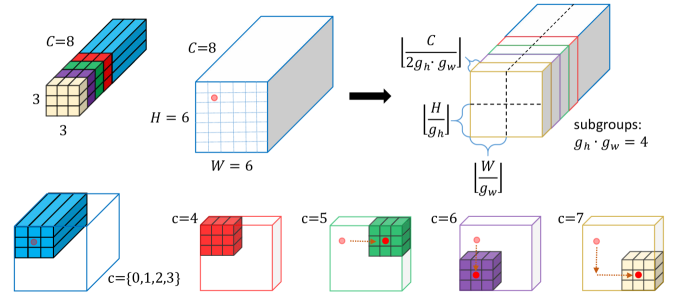
Figure 2: Illustration for 3$\times$3 global receptive convolution (GRC). This example shows how the GRC of 3$\times$3 filter size convolves a 6$\times$6$\times$8 input feature map, with the central pixel $(h_{0},w_{0})=(1,1)$ (shown as the light red dot in the top row). GRC divides the channel into two groups. For the group of $c=\{0,1,2,3\}$, standard convolution is applied, as in the blue cube at the bottom left. For the group of $c=\{4,5,6,7\}$, we further split it into $g_{h}\cdot g_{w}=4$ sub-group, with $g_{h}=g_{w}=2$. So each sub-group group has $\lfloor\frac{C}{2g_{h}\cdot g_{w}}\rfloor$=1 channel. Accordingly, the feature maps are divided into $g_{h}\cdot g_{w}=4$ sub-group, with spatial patch comprising $\frac{H}{g_{h}}\times\frac{W}{g_{w}}$ =3$\times$3 pixels. According to Eq. 6 or  7, $\hat{\mathcal{N}}=\{(0,0),(0,3),(3,0),(3,3)\}$. Given channel index like $c=5$, we can obtain $n=1$ via Eq. 8. Thus, for the 5th channel ($c=5$), the offset is $\hat{\mathcal{N}}_{1}=(0,3)$. This offset, shown as the dashed arrow in the bottom row, is then added to $(h_{0},w_{0})=(1,1)$ to shift the central sampling location. This leads to the new central sampling location of $(1,4)$. Centering on this new location, the convolution is applied in the 5th channel-wise sub-group, as shown in the green cube.

3.2 Global Receptive Convolution

We propose an effective and efficient convolution, dubbed global receptive convolution (GRC). The GRC provides global receptive field for convolutional filters without introducing any extra learnable parameters. The key to achieving this is to make different channels of a convolutional filter have different grid sampling locations across the whole input feature map. Specifically, we first divide the channels of the $W$ into two groups. Each group has equal channels by default, i.e., $\frac{C}{2}$. The equal channels are based on the assumption that the original location information and global context are equally important. We believe that this is a reasonable assumption when no prior knowledge of the dataset is available. For the group of $c=\{0,...,\frac{C}{2}-1\}$, we do standard convolution as in Eq. 1 and  2 to capture original location information. For the group of $c=\{\frac{C}{2},...,C-1\}$, we elaborately design its grid sampling locations, i.e., $\hat{\mathcal{N}}$, for global receptive field. $\hat{\mathcal{N}}$ will be introduced later. Then, the GRC is formulated as

$$F^{\prime}(h_{0},w_{0}) =\sum_{c=0}^{\frac{C}{2}-1}\sum_{(h,w)\in\mathcal{N}}W(c,h,w)*F(h_{0}+h,w_{0}+w,c)$$ (4)

$$+\sum_{c=\frac{C}{2}}^{C-1}\sum_{(\hat{h},\hat{w})\in\hat{\mathcal{N}}}\sum_{(h,w)\in\mathcal{N}}W(c,h,w)*$$

$$F(h_{0}+\hat{h}+h,w_{0}+\hat{w}+w,c),$$

where $\mathcal{N}$ is the same as Eq. 2. The first term is standard convolution as in Eq. 1 except that the summation over channel $c$ is from 0 to $\frac{C}{2}-1$. This term keeps the original location information for the pixel-wise representation (i.e., for the feature representation of the central pixels at $(h_{0},w_{0})$). In the second term, $\hat{\mathcal{N}}$ controls the central sampling location for GRC. The offsets $(\hat{h},\hat{w})$ in $\hat{\mathcal{N}}$ shift the central location from $(h_{0},w_{0})$ to other locations according to the channel index $c$. In this way, the offsets can enable different grid sampling locations for capturing global context information. The design of the offsets will be detailed in the next paragraph. Finally, the global context information is integrated into pixel-wise representations by summing these two terms. See Figure 2 for an illustration.

The offsets $\hat{h},\hat{w}$ control the shifted sampling locations. They are obtained by the following steps. We further split the group of $c=\{\frac{C}{2},...,C-1\}$ into $g_{h}\cdot g_{w}$ sub-groups. So, each sub-group has $\lfloor\frac{C}{2g_{h}\cdot g_{w}}\rfloor$ channels. Correspondingly, we split the feature map into $g_{h}\cdot g_{w}$ patches along the spatial dimension, with each patch containing $\lfloor\frac{H}{g_{h}}\rfloor\cdot\lfloor\frac{W}{g_{w}}\rfloor$ pixels. Then the offsets are defined as

$$\hat{h}=i\cdot\lfloor\frac{H}{g_{h}}\rfloor,\quad\hat{w}=j\cdot\lfloor\frac{W}{g_{w}}\rfloor,$$ (5)

where $i,j$ are patch indexes. They are integers that control the offsets, with $i\in[0,g_{h}-1],j\in[0,g_{w}-1]$. We will include the patch indexes $i,j$ to $\hat{h},\hat{w}$ for better clarity. This leads to $\hat{h}_{i},\hat{w}_{j}$. Now we can obtain $\hat{\mathcal{N}}$ by

$$\hat{\mathcal{N}}=\cup_{i,j}\{(\hat{h}_{i},\hat{w}_{j})\}.$$ (6)

More specifically, $\hat{\mathcal{N}}$ enumerates all the possible combinations of $i,j$, i.e.,

$$\hat{\mathcal{N}}= \left\{(0,0),\left(0,\lfloor\frac{W}{g_{w}}\rfloor\right),...,\right.$$ (7)

$$\left.\left((g_{h}-2)\cdot\lfloor\frac{H}{g_{h}}\rfloor,(g_{w}-1)\cdot\lfloor\frac{W}{g_{w}}\rfloor\right),\right.$$

$$\left.\left((g_{h}-1)\cdot\lfloor\frac{H}{g_{h}}\rfloor,(g_{w}-1)\cdot\lfloor\frac{W}{g_{w}}\rfloor\right)\right\}.$$

$\hat{\mathcal{N}}$ comprises $g_{h}\cdot g_{w}$ offset coordinates in total. It almost covers the whole input feature map, i.e., $H\times W$, thus providing a global receptive field for GRC. Recall that the key in GRC is to make different channels have different grid sampling locations. Hence, we choose different offset coordinates in $\hat{\mathcal{N}}$ according to the channel index $c$, or equivalently according to the channel-wise sub-group index $n$. Given $c$, $n$ can be formulated as

$$n=\begin{cases}0,\text{ if }\frac{C}{2}\leq c<\frac{C}{2}+\lfloor\frac{C}{2g_{h}\cdot g_{w}}\rfloor\\ 1,\text{ if }\frac{C}{2}+\lfloor\frac{C}{2g_{h}\cdot g_{w}}\rfloor\leq c<\frac{C}{2}+2\cdot\lfloor\frac{C}{2g_{h}\cdot g_{w}}\rfloor.\\ ...\\ (g_{h}\cdot g_{w}-1),\text{ if }\frac{C}{2}+(g_{h}\cdot g_{w}-1)\lfloor\frac{C}{2g_{h}\cdot g_{w}}\rfloor\leq c<C\end{cases}$$ (8)

The $n$-th sub-group of channels corresponds to the $n$-th offset coordinates of $\hat{\mathcal{N}}$, denoted as $\hat{\mathcal{N}}_{n}$. Therefore, different channel groups have different offset coordinates, resulting in different shifted sampling locations.

To sum up, the second term in Eq. 4 can be re-written as

$$\sum_{n=0}^{g_{h}\cdot g_{w}-1}\sum_{c=c_{n}}^{c_{n+1}}\sum_{(\hat{h},\hat{w})\in\hat{\mathcal{N}}_{n}}\sum_{(h,w)\in\mathcal{N}}W(c,h,w)*$$ (9)

$$F(h_{0}+\hat{h}+h,w_{0}+\hat{w}+w,c)$$

where $c_{n}=\frac{C}{2}+n\cdot\lfloor\frac{C}{2g_{h}\cdot g_{w}}\rfloor$.

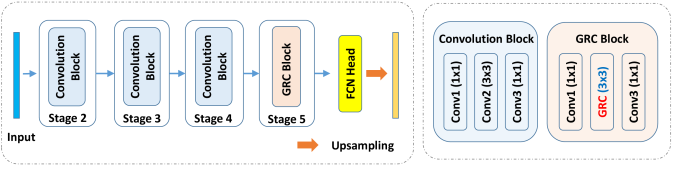
Figure 3: The architecture of FCN+. As in FCN [20], FCN+ combines coarse high-level information with fine low-level information. FCN+ adopts a ResNet backbone which has five residual stages (Stage 1 omitted for simplicity). The implementation of FCN head can refer to MMSegmentation [8]. The last stage of FCN+ is replaced with GRC-based residual blocks.

3.3 Improve GRC for Efficiency

We have elaborate on how to conduct GRC using a single filter, but note that the GRC contains $C^{\prime}$ filters ($C^{\prime}$ is omitted in Eq. 1). Shifting central sampling locations of all the $C^{\prime}$ filters one by one, with each shifting operation being channel-dependent, is memory expensive and inefficient for parallel computation. Therefore, we further simplify the implementation of GRC to improve its efficiency by assuming that the offsets for shifting are the same for these $C^{\prime}$ filters. That is, they are channel-dependent but filter-independent. Then, the simplification is based on the finding that shifting the central sampling locations of convolutional filters is equivalent to shifting the feature map because the motion is relative. Concretely, for each sub-group to be shifted, we keep the central sampling location the same as the standard convolution but shift the feature map of such sub-group according to the offsets. Formally, we can re-write the second term in Eq. 4 as

$$\sum_{c=\frac{C}{2}}^{C-1}\sum_{(h,w)\in\mathcal{N}}W(c,h,w)*\hat{F}(h_{0}+h,w_{0}+w,c),$$ (10)

$$\text{where}\quad\hat{F}(h_{0},w_{0},c)=F(h_{0}+h(c),w_{0}+w(c),c).$$ (11)

Eq. 10 is standard convolution but its feature map is transformed, denoted as $\hat{F}$. $\hat{F}$ groups and then shifts the $\frac{C}{2}\sim(C-1)$-th channels of original feature map $F$ according to Eq. 11, where $h(c),w(c)$ are channel-dependent shifting functions. $h(c)$ is defined as

$$h(c)=n\cdot\lfloor\frac{C}{2g_{h}\cdot g_{w}}\rfloor,$$ (12)

where $n$ is channel-dependent, defined in Eq. 8. Similarly, we can obtain $w(c)$.

To sum up, we can first shift half channels, i.e., the $\frac{C}{2}\sim(C-1)$-th channels, of the original feature maps according to Eq. 11 & 12. The feature shifting will be conducted $g_{h}\cdot g_{w}$ times, much less than shifting filters (this will be $g_{h}\cdot g_{w}\cdot C^{\prime}$ times). Then, we can simply apply standard convolution via Eq. 10 to facilitate parallel computation. Due to fewer shifting operations and parallel computation, feature map shifting is much more efficient. In practice, we implement our GRC by shifting the feature maps.

3.4 FCN+

Our GRC can be used to replace the standard convolution in popular semantic segmentation networks like fully convolutional network (FCN) [20]. With this modification, we turn FCN into FCN+, which favorably improves the segmentation performance over FCN. In this section, we will detail the FCN+.

As shown in Figure 3, FCN+ has the same architecture as FCN, which exploits deep convolutional neural networks (CNNs) to extract features for objects and scenes. To obtain multi-scale representations, FCN+ further aggregates feature maps of different spatial resolutions from hierarchical layers. The backbone feature extractor has four stages, each stage comprising several residual blocks [16]. We apply the GRC in the last stage (Stage 5) by replacing the 2nd convolution in a residual block with GRC, called a GRC block. The design choice of the GRC block will be evaluated in experiments.

4 Experiments

In this section, we conduct extensive experiments on PASCAL VOC 2012 [11], Cityscapes [9], and ADE20K [36] to justify the effectiveness of our GRC and FCN+.

4.1 Experimental Setting

Datasets and protocols. (1) PASCAL VOC 2012 [11] is a popular semantic segmentation dataset. It has 21 classes (including a background class), with 1,464 images for training, 1,449 for validation, and 1,456 for testing. Most previous works [5, 7, 32, 15, 14] adopt its augmented training set provided by [13] which comprises 10,582 training samples. Following these works, we use this augmented version as our training set. (2) Cityscapes [9] is a large-scale dataset for semantic understanding of urban street scenes. It consists of 5,000 fine annotated images and 20,000 annotated images from 30 classes. These images are captured in 50 different cities, covering different seasons and weather conditions. (3) ADE20K [36] is one of the most challenging datasets for semantic segmentation. It is challenging mainly due to its diverse and complex scenes as well as a large number of classes (i.e., 150 classes). There are 20K, 2K, and 3K images for training, validation and testing respectively.

Training details. At the training stage, we randomly flip and scale the input images as data augmentation, with a scale ratio in $[0.5,2]$. We then set the crop size to 512$\times$512 for PASCAL VOC 2012 and ADE20K, and 512$\times$1024 for Cityscapes. Each mini-batch contains 32 cropped images. Following  [20], we use ImageNet [24] pre-trained ResNet-101 [16] as our backbone model (unless otherwise stated). We remove stride and set dilation rates 2 and 4 for the last two stages. By default, we apply the GRC in the last stage of ResNet by replacing the 2nd convolution layer in a residual block with our GRC. The hyper-parameters for sub-group in GRC is $g_{h}=g_{w}$=4. To make the image size be divided evenly by the sub-group number, we use sliding windows empirically. Then, the whole model is optimized with momentum-based stochastic gradient descent (SGD). The momentum is 0.9 and the weight decay is 0.0001. The initial learning rate is 0.01 for all these datasets. The learning rate is then reduced according to different training iterations: $(1-\frac{iter}{total\_iter})^{power}$, where $power$ is 0.9. The whole training process takes 40K iterations for PASCAL VOC 2012, 80K iterations for Cityscapes, and 160K iterations for ADE20K dataset.

For inference, we adopt single-scale for testing, and crop testing images to the same size. The prediction is then interpolated in a bi-linear way to keep its size the same as the input images. Finally, the mean of class-wise intersection over union (mIoU) is adopted as the evaluation metric. Our experiments are conducted based on PyTorch [21, 22] and MMSegmentation [8].

4.2 Results on ADE20K

We first conduct comprehensive ablation studies on ADE20K to show the effectiveness of our FCN+ and global receptive convolution (GRC). Then we compare the FCN+ with other state-of-the-art methods.

GRC at different stages. By default, we apply the GRC to the last stage of ResNet. Since there are four stages in ResNet, we further investigate which stage is the best choice. The results are shown in Table 1. It is observed that the GRC at the last stage works best, probably because the last stage contains more high-level semantic information, thus can provide better global context.

Table 1: GRC vs. a variant of GRC at different stages of ResNet. The variant of GRC applies the offset-based convolution to all the channels. ‘S’ denotes the Stage in ResNet.

Stages	S5	S4-5	S3-5	S2-5
GRC	45.72	45.12	45.39	44.81
Variant of GRC	45.52	43.88	42.21	42.15

Table 2: Comparison of GRC with deformable convolution.

Methods	mIoU
GRC	45.72
Deformable	44.10

Table 3: GRC at different layers of a residual block.

Positions	mIoU
Conv1 (1$\times$1)	45.31
Conv2 (3$\times$3)	45.72
Conv3 (1$\times$1)	45.39

Table 4: Sensitivity of the number of sub-groups $g$.

Sub-groups $g$	4	8	16
mIoU	45.72	45.07	45.74

GRC at different layers. We then explore where to insert GRC in a residual block of Stage 5. A residual block of ResNet-50 or ResNet-101 has three layers, as shown in the right panel of Figure 3. We take turns replacing each layer with our GRC and show their performance in Table 3. The results demonstrate that the GRC at the 2nd convolutional layer works best. This can be explained by that the GRC benefits more from 3$\times$3 convolution than 1$\times$1.

The necessity of keeping one group for standard convolution in GRC. Recall that in Eq. (4), the first term is the standard convolution which aims to keep the local pixel-wise information. To justify its effectiveness, we remove the standard convolution in GRC and apply the offset-based convolution in Eq. (9) to all the channels. This modification decreases the performance under different stage settings, as shown in the last row of Table 1. The degradation implies that (1) only utilizing the global context information is still not sufficient for accurate segmentation results; (2) the local pixel-wise information is necessary for better pixel-wise representation, which is of immense importance for dense prediction tasks.

Table 5: Segmentation results of state-of-the-art methods on PASCAL VOC 2012, Cityscapes and ADE20K. All the results are obtained based on MMSegmentation [8].

Methods	PASCAL VOC	Cityscapes	ADE20K
FCN [20]	69.91	75.13	39.91
PSPNet [33]	78.52	79.76	44.39
PSANet [34]	77.73	79.31	43.74
UperNet [27]	77.43	79.40	43.82
APCNet [15]	-	79.64	45.41
Non-local [26]	78.27	78.93	44.63
DeepLabV3 [6]	77.92	80.20	45.00
DeepLabV3+ [7]	78.62	80.97	45.47
CCNet [17]	77.87	78.87	43.71
ANN [38]	76.70	77.14	42.94
DNLNet [30]	-	80.41	44.25
DEST [28]	-	75.28	-
FCN+ (Ours)	79.42	80.53	45.74

Table 6: Comparison of FCN+ with FCN on ADE20K.

Methods	Backbone	mIoU
FCN	ResNet-50	36.10
FCN+	ResNet-50	44.54
FCN	ResNet-101	39.91
FCN+	ResNet-101	45.74

Sensitivity of the number of sub-groups in GRC. In Eq. (5) and  (8), we have the two hyper-parameters for spatial-wises and channel-wise grouping, i.e., $g_{h},g_{w}$. They determine the total number of sub-groups for channels and spatial patches. In practice, the input images can sometimes be cropped to have the same height and width, leading to $H=W$. Thus, it is generally reasonable to set $g_{h}=g_{w}$ to reduce the number of hyper-parameters. Then we define $g=g_{h}=g_{w}$ and evaluate the sensitivity of $g$ in Table 4. We observe that the performance is stable. Though $g$ should be set according to channel depth and the size of feature maps, generally $g\in\{4,8,16\}$ is recommended.

GRC vs. deformable convolutions. In Table 2, we compare our GRC with deformable convolution (standard convolution has been compared in Table 6). For a fair comparison, we only replace the GRC with the deformable convolution while keeping all the other settings the same. We can see from Table 2 that our GRC is clearly better than this competitor. This suggests the superiority of our GRC in enlarging the receptive field.

FCN+ vs. FCN. We compare our FCN+ with the baseline method, i.e., FCN, in Table 6. We can see that replacing the standard convolution with our proposed GRC can increase the mIoU by 8.44% for ResNet-50, and 6.83% for ResNet-101. It is also noteworthy that our FCN+ does not introduce any extra parameters or FLOPs to FCN (though not shown in the table). This makes our FCN+ highly efficient. The performance improvement results from the global receptive field of GRC, which can exploit the global context for better pixel-wise representations. These comparisons verify the efficiency and efficacy of our FCN+.

Until now, we have investigated three cases of different channel numbers. They are A: FCN based on standard convolution with all channels having original sampling locations; B: FCN+ based on GRC with evenly separated channels; C: Variant of GRC with all channels having shifted sampling locations. Table 6 shows A vs. B, where B (FCN+) is clearly better than A (FCN). Besides, Table 1 shows the results of B (1st row, GRC) vs. C (2nd row) where B beats C. Thus, evenly separating channels is better than the other two design choices.

Comparison with the state of the art. Finally, we compare our FCN+ with other state-of-the-art methods in Table 5. We can see that our FCN+ surpasses these methods based on (1) standard convolution [20, 14], (2) the dilated convolution [7, 15], and (3) the attention [26, 17, 38]. Notably, our FCN+ outperforms the baseline method FCN [20] by a clear margin. In addition, Non-local [26] is another work that captures global context via complicated matrix multiplication, leading to more parameters and FLOPs. While GRC uses global sparse sampling without introducing any parameters or FLOPs but has better performance (45.74 vs. 44.63). Finally, our FCN+ is more efficient than these using multiple dilated convolutions or learning offsets for each sampling location. We owe the efficacy and efficiency of FCN+ to the global receptive field brought by GRC.

4.3 Results on Cityscapes

Table 5 also shows the comparison on Cityscapes. It is clear that our FCN+ improves the FCN by 5.40%, and achieves comparable or better performance than all the competitors. It is worth noting that our FCN+ beats the latest DEST [28], which adopts a strong transformer backbone (SMIT-B5), by 5.25. The superiority attributes to the GRC for capturing global context. Compared with DeepLabV3+ [7], our FCN+ achieves slightly worse performance, but FCN+ does not need complicated decoders as in DeepLabV3+, thus more efficient. This verifies that even without complicated decoders, the FCN+ can effectively deal with the challenges of objects’ scale variation and confusion boundaries.

4.4 Results on PASCAL VOC 2012

We further evaluate our FCN+ on PASCAL VOC 2012 and compare it with other state-of-the-art methods in Table 5. FCN+ increases the performance of FCN by 9.51%, which demonstrates the superiority of GRC to the standard convolution. Compared with other methods, the FCN+ also obtains comparable or even better performance. The superior performance of FCN+ illustrates that GRC can handle the challenge of complex scenes and diverse classes in PASCAL VOC 2012.

4.5 Limitations

Though our GRC is efficient and effective, it relies on artificial grouping and introduces a hyper-parameter $g(=g_{w}=g_{h})$. These groups can sometimes be sub-optimal, e.g., a specific large object can be spatially grouped into several sub-groups. This can be alleviated by designing content-dependent grouping— automatically grouping according to content can be more effective and save time for hyper-parameter tuning.

5 Conclusion

In this paper, we find that a size-fixed filter cannot capture global receptive field mainly because the grid sampling locations of such a filter are limited to a fixed local spatial coordinate. To address this issue, we argue that the grid sampling locations of convolution should be dependent on both spatial coordinates and different channels. Based on this, we propose a novel global receptive convolution (GRC) to provide global receptive field for convolution. More importantly, the GRC can integrate the global context into the original location information of each pixel for better dense prediction results. We further incorporate the GRC into FCN and propose FCN+. We show that FCN+ can outperform state-of-the-art methods on some popular semantic segmentation datasets, such as PASCAL VOC 2012, Cityscapes, and ADE20K.

References

- [1] Vijay Badrinarayanan, Alex Kendall, and Roberto Cipolla. Segnet: A deep convolutional encoder-decoder architecture for image segmentation. IEEE T-PAMI, 39(12):2481–2495, 2017.
- [2] Abhishek Chaurasia and Eugenio Culurciello. Linknet: Exploiting encoder representations for efficient semantic segmentation. In IEEE Visual Communications and Image Processing (VCIP), pages 1–4. IEEE, 2017.
- [3] Jieneng Chen, Yongyi Lu, Qihang Yu, Xiangde Luo, Ehsan Adeli, Yan Wang, Le Lu, Alan L Yuille, and Yuyin Zhou. Transunet: Transformers make strong encoders for medical image segmentation. arXiv preprint arXiv:2102.04306, 2021.
- [4] Liang-Chieh Chen, George Papandreou, Iasonas Kokkinos, Kevin Murphy, and Alan L Yuille. Semantic image segmentation with deep convolutional nets and fully connected crfs. arXiv preprint arXiv:1412.7062, 2014.
- [5] Liang-Chieh Chen, George Papandreou, Iasonas Kokkinos, Kevin Murphy, and Alan L Yuille. Deeplab: Semantic image segmentation with deep convolutional nets, atrous convolution, and fully connected crfs. IEEE T-PAMI, 40(4):834–848, 2017.
- [6] Liang-Chieh Chen, George Papandreou, Florian Schroff, and Hartwig Adam. Rethinking atrous convolution for semantic image segmentation. arXiv preprint arXiv:1706.05587, 2017.
- [7] Liang-Chieh Chen, Yukun Zhu, George Papandreou, Florian Schroff, and Hartwig Adam. Encoder-decoder with atrous separable convolution for semantic image segmentation. In ECCV, pages 801–818, 2018.
- [8] MMSegmentation Contributors. MMSegmentation: Openmmlab semantic segmentation toolbox and benchmark. https://github.com/open-mmlab/mmsegmentation, 2020.
- [9] Marius Cordts, Mohamed Omran, Sebastian Ramos, Timo Rehfeld, Markus Enzweiler, Rodrigo Benenson, Uwe Franke, Stefan Roth, and Bernt Schiele. The cityscapes dataset for semantic urban scene understanding. In CVPR, pages 3213–3223, 2016.
- [10] Jifeng Dai, Haozhi Qi, Yuwen Xiong, Yi Li, Guodong Zhang, Han Hu, and Yichen Wei. Deformable convolutional networks. In ICCV, pages 764–773, 2017.
- [11] Mark Everingham, Luc Van Gool, Christopher KI Williams, John Winn, and Andrew Zisserman. The pascal visual object classes (voc) challenge. IJCV, 88(2):303–338, 2010.
- [12] Jun Fu, Jing Liu, Haijie Tian, Yong Li, Yongjun Bao, Zhiwei Fang, and Hanqing Lu. Dual attention network for scene segmentation. In CVPR, pages 3146–3154, 2019.
- [13] Bharath Hariharan, Pablo Arbeláez, Ross Girshick, and Jitendra Malik. Hypercolumns for object segmentation and fine-grained localization. In CVPR, pages 447–456, 2015.
- [14] Junjun He, Zhongying Deng, and Yu Qiao. Dynamic multi-scale filters for semantic segmentation. In ICCV, pages 3562–3572, 2019.
- [15] Junjun He, Zhongying Deng, Lei Zhou, Yali Wang, and Yu Qiao. Adaptive pyramid context network for semantic segmentation. In CVPR, pages 7519–7528, 2019.
- [16] Kaiming He, Xiangyu Zhang, Shaoqing Ren, and Jian Sun. Deep residual learning for image recognition. In CVPR, pages 770–778, 2016.
- [17] Zilong Huang, Xinggang Wang, Lichao Huang, Chang Huang, Yunchao Wei, and Wenyu Liu. Ccnet: Criss-cross attention for semantic segmentation. In ICCV, pages 603–612, 2019.
- [18] Yanwei Li, Lin Song, Yukang Chen, Zeming Li, Xiangyu Zhang, Xingang Wang, and Jian Sun. Learning dynamic routing for semantic segmentation. In CVPR, pages 8553–8562, 2020.
- [19] Wei Liu, Andrew Rabinovich, and Alexander C Berg. Parsenet: Looking wider to see better. arXiv preprint arXiv:1506.04579, 2015.
- [20] Jonathan Long, Evan Shelhamer, and Trevor Darrell. Fully convolutional networks for semantic segmentation. In CVPR, pages 3431–3440, 2015.
- [21] Adam Paszke, Sam Gross, Soumith Chintala, Gregory Chanan, Edward Yang, Zachary DeVito, Zeming Lin, Alban Desmaison, Luca Antiga, and Adam Lerer. Automatic differentiation in pytorch. 2017.
- [22] Adam Paszke, Sam Gross, Francisco Massa, Adam Lerer, James Bradbury, Gregory Chanan, Trevor Killeen, Zeming Lin, Natalia Gimelshein, Luca Antiga, et al. Pytorch: An imperative style, high-performance deep learning library. NeurIPS, 32, 2019.
- [23] Olaf Ronneberger, Philipp Fischer, and Thomas Brox. U-net: Convolutional networks for biomedical image segmentation. In International Conference on Medical image computing and computer-assisted intervention, pages 234–241. Springer, 2015.
- [24] Olga Russakovsky, Jia Deng, Hao Su, Jonathan Krause, Sanjeev Satheesh, Sean Ma, Zhiheng Huang, Andrej Karpathy, Aditya Khosla, Michael Bernstein, et al. Imagenet large scale visual recognition challenge. IJCV, 115(3):211–252, 2015.
- [25] Panqu Wang, Pengfei Chen, Ye Yuan, Ding Liu, Zehua Huang, Xiaodi Hou, and Garrison Cottrell. Understanding convolution for semantic segmentation. In WACV, pages 1451–1460. Ieee, 2018.
- [26] Xiaolong Wang, Ross Girshick, Abhinav Gupta, and Kaiming He. Non-local neural networks. In CVPR, pages 7794–7803, 2018.
- [27] Tete Xiao, Yingcheng Liu, Bolei Zhou, Yuning Jiang, and Jian Sun. Unified perceptual parsing for scene understanding. In ECCV, pages 418–434, 2018.
- [28] John Yang, Le An, Anurag Dixit, Jinkyu Koo, and Su Inn Park. Depth estimation with simplified transformer. CVPR Workshop, 2022.
- [29] Maoke Yang, Kun Yu, Chi Zhang, Zhiwei Li, and Kuiyuan Yang. Denseaspp for semantic segmentation in street scenes. In CVPR, pages 3684–3692, 2018.
- [30] Minghao Yin, Zhuliang Yao, Yue Cao, Xiu Li, Zheng Zhang, Stephen Lin, and Han Hu. Disentangled non-local neural networks. In ECCV, pages 191–207. Springer, 2020.
- [31] Yuhui Yuan, Lang Huang, Jianyuan Guo, Chao Zhang, Xilin Chen, and Jingdong Wang. Ocnet: Object context network for scene parsing. arXiv preprint arXiv:1809.00916, 2018.
- [32] Hang Zhang, Kristin Dana, Jianping Shi, Zhongyue Zhang, Xiaogang Wang, Ambrish Tyagi, and Amit Agrawal. Context encoding for semantic segmentation. In CVPR, pages 7151–7160, 2018.
- [33] Hengshuang Zhao, Jianping Shi, Xiaojuan Qi, Xiaogang Wang, and Jiaya Jia. Pyramid scene parsing network. In CVPR, pages 2881–2890, 2017.
- [34] Hengshuang Zhao, Yi Zhang, Shu Liu, Jianping Shi, Chen Change Loy, Dahua Lin, and Jiaya Jia. Psanet: Point-wise spatial attention network for scene parsing. In ECCV, pages 267–283, 2018.
- [35] Sixiao Zheng, Jiachen Lu, Hengshuang Zhao, Xiatian Zhu, Zekun Luo, Yabiao Wang, Yanwei Fu, Jianfeng Feng, Tao Xiang, Philip HS Torr, et al. Rethinking semantic segmentation from a sequence-to-sequence perspective with transformers. In CVPR, pages 6881–6890, 2021.
- [36] Bolei Zhou, Hang Zhao, Xavier Puig, Sanja Fidler, Adela Barriuso, and Antonio Torralba. Scene parsing through ade20k dataset. In CVPR, pages 633–641, 2017.
- [37] Zongwei Zhou, Md Mahfuzur Rahman Siddiquee, Nima Tajbakhsh, and Jianming Liang. Unet++: A nested u-net architecture for medical image segmentation. In Deep learning in medical image analysis and multimodal learning for clinical decision support, pages 3–11. Springer, 2018.
- [38] Zhen Zhu, Mengde Xu, Song Bai, Tengteng Huang, and Xiang Bai. Asymmetric non-local neural networks for semantic segmentation. In ICCV, pages 593–602, 2019.