Complete positivity violation of the reduced dynamics in higher-order quantum adiabatic elimination

Abstract

This paper discusses quantum adiabatic elimination, which is a model reduction technique for a composite Lindblad system consisting of a fast decaying sub-system coupled to another sub-system with a much slower timescale. Such a system features an invariant manifold that is close to the slow sub-system. This invariant manifold is reached subsequent to the decay of the fast degrees of freedom, after which the slow dynamics follow on it. By parametrizing invariant manifold, the slow dynamics can be simulated via a reduced model. To find the evolution of the reduced state, we perform the asymptotic expansion with respect to the timescale separation. So far, the second-order expansion has mostly been considered. It has then been revealed that the second-order expansion of the reduced dynamics is generally given by a Lindblad equation, which ensures complete positivity of the time evolution. In this paper, we present two examples where complete positivity of the reduced dynamics is violated with higher-order contributions. In the first example, the violation is detected for the evolution of the partial trace without truncation of the asymptotic expansion. The partial trace is not the only way to parametrize the slow dynamics. Concerning this non-uniqueness, it was conjectured in [R. Azouit, F. Chittaro, A. Sarlette, and P. Rouchon, Quantum Sci. Technol. 2, 044011 (2017)] that there exists a parameter choice ensuring complete positivity. With the second example, however, we refute this conjecture by showing that complete positivity cannot be restored in any choice of parametrization. We discuss these results in terms of unavoidable correlations, in the initial states on the invariant slow manifold, between the fast and the slow degrees of freedom.

I Introduction

Any quantum system should be treated as an open system. One of the reasons is that perfect isolation of a quantum system is unrealistic experimentally and the influence of a surrounding environment needs to be taken into account. Besides, perfectly isolated systems cannot be used for the purpose of quantum control. In order to control or read out a quantum state, coupling to another system is unavoidable. A state of an open quantum system is represented by a density matrix. To describe its evolution, various approximation methods have been developed so far. One of the most widely used method is based on the Markov assumption. Starting from a system-environment Hamiltonian, the Born-Markov-Secular approximations lead to a Lindblad equation Breuer02 .

Lindblad equations can also be derived mathematically by imposing axiomatic conditions on the time evolution map. It is reasonable to assume that the time evolution preserves the properties of density matrices, namely they are Hermitian, unit-trace, and positive-semidefinite for the entire evolution. The condition of positivity is usually replaced by complete positivity NielsenChuang . The complete positivity requirement in physics stems from the fact that a density matrix of an open quantum system is a reduced one, and the total density matrix including an environment should also be positive semidefinite. One can show that the evolution of a density matrix is governed by a Lindblad equation if and only if the time evolution map is a one-parameter semigroup ($\{\Lambda_{t}\}_{t\geq 0}$ satisfying $\Lambda_{t}\circ\Lambda_{s}=\Lambda_{t+s}$ for all $t,s\geq 0$), the elements of which are trace preserving completely positive maps for all $t\geq 0$ GKS ; Lindblad ; Havel03 . Note that the semigroup property is associated with the Markov assumption Breuer02 .

In this paper, we consider a composite open quantum system where the total evolution is governed by a Lindblad equation. The composite system is assumed to consist of a fast decaying sub-system being weakly coupled to another system with a slower time scale. In this setting, the time evolution typically starts with decay of fast degrees of freedom followed by a slower evolution of the remaining slow degrees of freedom. In capturing the latter dynamics, thus, the fast degrees of freedom can be discarded. This model reduction technique is known in quantum physics as adiabatic elimination and goes back to singular perturbation theory (see, e.g., Kotovic-review ). Thanks to the linearity of Lindblad equations, there exists in fact an invariant linear subspace, associated with the slow eigenvalues of the overall system, on which this dynamics rigorously takes place.

Adiabatic elimination offers two noteworthy aspects when applied to quantum physics problems. Firstly, it provides a model reduction technique for composite Lindblad systems. By discarding the fast degrees of freedom, the slow dynamics can be described via a reduced model. This enables simulations of large-dimensional systems that are otherwise infeasible. Secondly, adiabatic elimination allows for reservoir engineering. By crafting the coupling between the two sub-systems, we can design the dissipative dynamics of the slow evolution after the decay. This aspect is important in recent developments of quantum technologies, because dissipation is not necessarily the enemy of quantum technology, but can be leveraged to control a quantum state. These aspects of adiabatic elimination can be seen in previous studies, such as Karabanov15 ; Antoine21 ; Wiseman93 ; Mazyar14 .

For general settings, adiabatic elimination was formulated using degenerate perturbation theory in Zanardi16 . Later, Azouit17 provided a geometric picture based on center manifold theory Fenichel79 . The system according to this theory does exactly feature an invariant manifold corresponding to slow dynamics, and hence we can view the model reduction to slow degrees of freedom as trying to approximate this manifold and the evolution once the system is initialized on it. To formulate the model reduction based on this picture, we parametrize the degrees of freedom on an invariant manifold. We then seek to find two maps; one describing the time evolution of the parameters and the other assigning the parametrization the solution of the Lindblad equation, that is, the density matrix of the total system. To calculate these maps approximately for general problems, the asymptotic expansion with respect to the timescale separation is performed. In this way, Azouit17 established a methodology to calculate higher-order contributions systematically. Recently, this approach was extended to a periodically driven system where the driving frequency is comparable to the fast timescale, while the amplitude is in the order of the slow timescale Michiel22 .

In the geometric approach, adiabatic elimination includes a gauge degree of freedom associated with the non-uniqueness of the parametrization. If the slow dynamics is parametrized via a density matrix, then one expects as a physical requirement that the two maps introduced above should preserve the quantum structure. This expectation is behind the conjecture made in Azouit17 ; the authors conjectured the existence of a gauge choice such that the reduced dynamics is governed by a Lindblad equation and the assignment is a trace preserving completely positive map (also called a Kraus map Choi75 ) up to any order of the asymptotic expansion. So far, this has been proved to be true for a general class of settings up to the second-order expansion; it was shown in Azouit17 that the evolution equation admits a Lindblad equation and in AzouitThesis that there always exists a gauge choice ensuring the Kraus map assignment. Studies of the higher order contributions have been limited so far. For a two qubit system, Alain20 reported an example supporting the conjecture at any order. Similar but different issues were discussed in Burgarth21 . The authors extended the Schrieffer-Wolff transformation to open quantum systems. They then found that the effective adiabatic generator, which has the the same block matrix structure as the unperturbed part and provides a first-order approximation of the total dynamics for all the time, cannot in general be put in the Lindblad form, even without truncation in the perturbation series, due to an unavoidable negative coefficient in front of one of the dissipators. We note that they investigated the effective generator for the total system, while the conjecture is about the generator for the reduced system. In our picture, it is clear that the total dynamics follows a Lindblad equation. The question is whether it can be split up into a Lindblad equation on a Hilbert space equivalent to the slow sub-system, and a Kraus mapping of this parameterization to the total system.

In this paper, we challenge this conjecture by taking into account higher-order contributions beyond second-order. We emphasize that recent advances of quantum technologies warrant accurate simulation of the slow dynamics. Thus, understanding of higher-order contributions is increasingly in need. We specifically consider two examples to investigate the conjecture. In the first example, which is a three-level system dispersively coupled to a strongly dissipative qubit, adiabatic elimination can be performed without any truncation of the expansion series. In such all-order analysis, we show that parameterization of the slow manifold via the partial trace of the total density matrix with respect to the fast sub-system yields a non-Lindblad equation violating even positivity, let alone complete positivity, of the time evolution. We stress that this is a result for the partial trace parametrization and, according to the conjecture, there might exist a different gauge choice in which the Lindblad form is restored. To explore the capacity of the gauge degree of freedom, we consider a qubit resonantly coupled to a strongly dissipative oscillator as the second example. In this example, we can rigorously prove that, with fourth-order contributions, complete positivity of the reduced dynamics cannot be attained, whatever the gauge choice is. Thus, this system serves as a counterexample to the conjecture. The proof utilizes a result in WPG10 which reveals a constraint on the spectrum of completely positive qubit maps. We discuss this complete positivity violation in terms of the correlation between the fast and slow degrees of freedom, which imposes a restriction on the initial state of the reduced system.

The paper is organized as follows. In Sec. II, the machinery of adiabatic elimination developed in Azouit17 is reviewed. To investigate role of the gauge degree of freedom, we derive how the time evolution and assignment maps are modified in different choices of gauge. In Sec. III, we consider a dispersively coupled system. For the partial trace, we show that complete positivity of the evolution is violated in the all-order analysis. Next in Sec. IV, we consider an oscillator-qubit system in which the dissipative oscillator system is eliminated. With this example, we prove the impossibility of restoring complete positivity by any gauge transformation. An interpretation of these findings are presented in Sec. V. Lastly, concluding remarks are made in Sec. VI.

II Adiabatic elimination

In this section, we review the machinery of adiabatic elimination developed in Azouit17 . We consider a system consisting of a fast decaying sub-system coupled to another sub-system with a slower timescale. Let $\mathscr{H}_{A}$ ($\mathscr{H}_{B}$) be the Hilbert space of the fast (slow) sub-system. The density matrix of the composite system, $\mathscr{H}_{A}\otimes\mathscr{H}_{B}$, denoted by $\rho$ follows a Lindblad equation,

$$\frac{d}{dt}\rho=\mathcal{L}_{A}\otimes\mathcal{I}_{B}(\rho)+\epsilon\mathcal{I}_{A}\otimes\mathcal{L}_{B}(\rho)+\epsilon\mathcal{L}_{\rm int}(\rho)\equiv\mathcal{L}_{\rm tot}(\rho).$$ (1)

For $\xi=A$ and $B$, $\mathcal{I}_{\xi}$ are the identity superoperators acting only to operators on $\mathscr{H}_{\xi}$. $\mathcal{L}_{A}$ is a Lindbladian acting only on $\mathscr{H}_{A}$ and generally reads

$$\mathcal{L}_{A}=-iH_{A}^{\times}+\sum_{k}\mathcal{D}[L_{A,k}],$$ (2)

with a Hamiltonian $H_{A}$ and jump operators $\{L_{A,k}\}$, all of which are operators on $\mathscr{H}_{A}$. We have also introduced the commutator superoperator $H^{\times}(\bullet)=H\bullet-\bullet H$ and the dissipator superoperator $\mathcal{D}[L](\bullet)=L\bullet L^{\dagger}-(L^{\dagger}L\bullet+\bullet L^{\dagger}L)/2$ for any operator $H$ and $L$. We assume that the evolution only with $\mathcal{L}_{A}$ exponentially converges to a unique steady state $\bar{\rho}_{A}$. In other words, among the spectrum of $\mathcal{L}_{A}$, the eigenvalue zero is simple and the other eigenvalues have strictly negative real part. $\mathcal{L}_{B}$ and $\mathcal{L}_{\rm int}$ are superoperators acting on $\mathscr{H}_{B}$ and $\mathscr{H}_{A}\otimes\mathscr{H}_{B}$, respectively, and are assumed to contain only Hamiltonian terms. Lastly, $\epsilon$ is a non-negative parameter representing the timescale separation. Physically, $\mathcal{L}_{A}$ and $\mathcal{L}_{B}$ describe the internal dynamics of $\mathscr{H}_{A}$ and $\mathscr{H}_{B}$, respectively, and $\mathcal{L}_{\rm int}$ determines how the two sub-systems interact.

As described in the Introduction section, the goal of adiabatic elimination is to find the slow dynamics on an invariant manifold. For linear equations such as a Lindblad equation, an invariant manifold is characterized by the (right) eigenoperators of the generator ($\mathcal{L}_{\rm tot}$ in Eq. (1)) whose eigenvalue has real part close to zero. Such a subspace is preserved by the operation of $\mathcal{L}_{\rm tot}$ and thus is invariant with respect to the time evolution map. We note that, when $\mathcal{L}_{\rm int}$ is nonzero, an invariant manifold does not exactly coincide with the slow sub-system $\mathscr{H}_{B}$ because of correlations building up between fast and slow sub-systems (see Sec. V for detailed discussions). To describe the slow dynamics, we parametrize the degrees of freedom on an invariant manifold. Following Azouit17 , we use a density matrix for the parametrization. As a mathematical model reduction technique, there is no preference in that choice. In applications to physics, on the other hand, it is convenient to employ a parametrization that facilitates interpretation of the slow dynamics. A suitable representation in this regard is a density matrix, since most studies of open quantum systems have been based on it. We note that the partial trace ${\rm tr}_{A}(\rho)$, with ${\rm tr}_{A}$ the trace over $\mathscr{H}_{A}$, has commonly been used to represent the reduced system Breuer02 ; NielsenChuang . This is a valid gauge choice, as far as the timescales are well separated (equivalently, $\epsilon\ll 1$). This choice plays a central role in the following discussions. For clear distinction, we denote the partial trace by $\rho_{B}={\rm tr}_{A}(\rho)$ and general parametrization by $\rho_{s}$.

Once the parametrization is fixed to $\rho_{s}$, we seek to find the following two maps. One, denoted by $\mathcal{L}_{s}$, describes the time evolution of $\rho_{s}$, namely $(d/dt)\rho_{s}=\mathcal{L}_{s}(\rho_{s})$. The other, denoted by $\mathcal{K}$, maps $\rho_{s}$ to the solution $\rho$ of the total Lindblad equation Eq. (1), $\rho=\mathcal{K}(\rho_{s})$. Throughout this paper, we assume that $\mathcal{K}$ and $\mathcal{L}_{s}$ are linear and time-independent (see below). Since $\rho$ satisfies Eq. (1), we obtain

$$\mathcal{K}(\mathcal{L}_{s}(\rho_{s}))=\mathcal{L}_{\rm tot}(\mathcal{K}(\rho_{s})),$$ (3)

from which we can determine $\mathcal{K}$ and $\mathcal{L}_{s}$ in principle. We call this relation the invariance condition in this paper.

Except special cases (see Sec. III), it is difficult to find $\mathcal{K}$ and $\mathcal{L}_{s}$ satisfying the invariance condition Eq. (3) exactly. To proceed, we assume $\epsilon\ll 1$ and perform the asymptotic expansions as

$$\mathcal{K}=\sum_{n=0}^{\infty}\epsilon^{n}\mathcal{K}_{n},\ \ \ \ \ \ \ \ \mathcal{L}_{s}=\sum_{n=0}^{\infty}\epsilon^{n}\mathcal{L}_{s,n}.$$ (4)

When $\epsilon=0$, the solution of Eq. (1) after the decay of the fast sub-system reads $\rho(t)=\bar{\rho}_{A}\otimes{\rm tr}_{A}(\rho(t=0))$ with the initial density matrix $\rho(t=0)$. Therefore, the zeroth elements are given by

$$\mathcal{K}_{0}(\rho_{s})=\bar{\rho}_{A}\otimes\rho_{s},\ \ \ \ \ \ \ \ \mathcal{L}_{s,0}(\rho_{s})=0.$$ (5)

The higher-order contributions can be obtained by substituting the expansions Eq. (4) into the invariance condition Eq. (3). The $n$-th order of $\epsilon$ reads

$$\bar{\rho}_{A}\otimes\mathcal{L}_{s,n}(\rho_{s})=\mathcal{L}_{A}\otimes\mathcal{I}_{B}(\mathcal{K}_{n}(\rho_{s})))+\mathcal{L}_{n}(\rho_{s}),$$ (6)

where we have introduced

$$\begin{gathered}\mathcal{L}_{n}(\rho_{s})=(\mathcal{I}_{A}\otimes\mathcal{L}_{B}+\mathcal{L}_{\rm int})(\mathcal{K}_{n-1}(\rho_{s}))\\ -\sum_{k=1}^{n-1}\mathcal{K}_{k}(\mathcal{L}_{s,n-k}(\rho_{s})).\end{gathered}$$

Since ${\rm tr}_{A}(\mathcal{L}_{A})=0$, the partial trace over $\mathscr{H}_{A}$ leads to $\mathcal{L}_{s,n}$ in the form

$$\mathcal{L}_{s,n}(\rho_{s})={\rm tr}_{A}(\mathcal{L}_{n}(\rho_{s})).$$ (7)

Eq. (6) can then be rearranged with known terms on the right hand side;

$$\mathcal{L}_{A}\otimes\mathcal{I}_{B}(\mathcal{K}_{n}(\rho_{s}))=\bar{\rho}_{A}\otimes\mathcal{L}_{s,n}(\rho_{s})-\mathcal{L}_{n}(\rho_{s}).$$ (8)

To solve this linear equation for $\mathcal{K}_{n}(\rho_{s})$, one needs to invert $\mathcal{L}_{A}$. Note that $\mathcal{L}_{A}$ is singular since one of the eigenvalues is zero. Thus, this linear equation is underdetermined. By identifying the Kernel of $\mathcal{L}_{A}\otimes\mathcal{I}_{B}$, $\mathcal{K}_{n}(\rho_{s})$ is determined only up to $\bar{\rho}_{A}\otimes{\rm tr}_{A}(\mathcal{K}_{n}(\rho_{s}))$ by solving (8). We introduce the undetermined part, $G_{n}={\rm tr}_{A}\circ\mathcal{K}_{n}$, which can be any superoperator on $\mathscr{H}_{B}$. This gauge degree of freedom is associated with the non-uniqueness of the parametrization. With $G_{n}(\rho_{s})$, $\mathcal{K}_{n}(\rho_{s})$ reads

$$\begin{gathered}\mathcal{K}_{n}(\rho_{s})=\mathcal{L}_{A}^{+}\otimes\mathcal{I}_{B}(\bar{\rho}_{A}\otimes\mathcal{L}_{s,n}(\rho_{s})-\mathcal{L}_{n}(\rho_{s}))\\ +\bar{\rho}_{A}\otimes G_{n}(\rho_{s}),\end{gathered}$$ (9)

where $\mathcal{L}_{A}^{+}$ is the Moore-Penrose inverse of $\mathcal{L}_{A}$. One way to calculate $\mathcal{L}_{A}^{+}$ by making use of the fact that the evolution only with $\mathcal{L}_{A}$ exponentially converges to a unique steady state was discussed in Azouit17 . We revisit their results using the vectorization method in Appendix A. Notice that the definition of the gauge superoperator is different from that in Azouit17 . In this paper, the choice $G_{n}=0\ (n=1,2,\dots)$ corresponds to the parametrization via the partial trace $\rho_{s}=\rho_{B}$.

From Eqs. (7) and (9), we can obtain $\mathcal{K}_{n}$ and $\mathcal{L}_{s,n}$ up to a desired order. From these equations, we see that $\mathcal{K}_{n}$ and $\mathcal{L}_{s,n+1}$ depend on $G_{1},\dots,G_{n}$. Therefore, $\mathcal{K}_{n}$ and $\mathcal{L}_{s,n+1}$ become, for instance, nonlinear functions of $\rho_{s}$ if so is even one of $G_{1},\dots,G_{n}$. To meet the conditions that $\mathcal{K}$ and $\mathcal{L}_{s}$ are linear and time-independent, we assume that $\{G_{n}\}$ have those properties.

From the definition of $G_{n}$, we find

$$\rho_{B}={\rm tr}_{A}(\rho)={\rm tr}_{A}(\mathcal{K}(\rho_{s}))=\rho_{s}+G(\rho_{s}),$$ (10)

with $G=\sum_{n=1}^{\infty}\epsilon^{n}G_{n}$. Throughout this paper, we assume that $(\mathcal{I}_{B}+G)$ is invertible, which is valid for $\epsilon\ll 1$ such that the truncation at a finite order is reasonable.

Let us next see how $\mathcal{K}$ and $\mathcal{L}_{s}$ for an arbitrary gauge choice are related to those for the partial trace. For the sake of clarity, we write the gauge dependence explicitly as $\mathcal{K}^{G}$ and $\mathcal{L}_{s}^{G}$. We note in advance that the following relations are results of general basis change and have nothing to do with the quantum structure. For $\mathcal{K}^{G}$, note $\rho=\mathcal{K}^{G}(\rho_{s})=\mathcal{K}^{G=0}(\rho_{B})$. Substituting Eq. (10) into the rightmost side gives

$$\mathcal{K}^{G}=\mathcal{K}^{G=0}\circ(\mathcal{I}_{B}+G).$$ (11)

For $\mathcal{L}_{s}^{G}$, the time evolution of the partial trace reads $\mathcal{L}_{s}^{G=0}(\rho_{B})=(d/dt)\rho_{B}=(d/dt)(\rho_{s}+G(\rho_{s}))=\mathcal{L}_{s}^{G}(\rho_{s})+G(\mathcal{L}_{s}^{G}(\rho_{s}))$. Comparing the leftmost and rightmost sides, we find $\mathcal{L}_{s}^{G=0}\circ(\mathcal{I}_{B}+G)=(\mathcal{I}_{B}+G)\circ\mathcal{L}_{s}^{G}$. From the existence of $(\mathcal{I}_{B}+G)^{-1}$, we obtain

$$\mathcal{L}_{s}^{G}=(\mathcal{I}_{B}+G)^{-1}\circ\mathcal{L}_{s}^{G=0}\circ(\mathcal{I}_{B}+G).$$ (12)

This indicates that the spectrum of $\mathcal{L}_{s}$ or the decay rate on an invariant manifold is independent of gauge choice. This is expected since the decay rate must not change depending on the way the slow dynamics is parametrized. Eqs. (11) and (12) are useful in analyzing possible transformations that the gauge degree of freedom can make (see Sec. IV).

As summarized in the Introduction section, the authors of Azouit17 conjectured the existence of a gauge choice leading to reduced dynamics described by a Lindbladian, $\sum_{j=0}^{n}\epsilon^{j}\mathcal{L}_{s,j}(\rho_{s})=-i[H_{s},\rho_{s}]+\sum_{k}\mathcal{D}[L_{s,k}](\rho_{s})$ with a Hamiltonian $H_{s}$ and jump operators $\{L_{s,k}\}$, and assignment described by a Kraus map, $\sum_{j=0}^{n}\epsilon^{j}\mathcal{K}_{j}(\rho_{s})=\sum_{k}M_{k}\rho_{s}M_{k}^{\dagger}$ with operators $M_{k}:\mathscr{H}_{B}\to\mathscr{H}_{A}\otimes\mathscr{H}_{B}$, up to $\epsilon^{n}$ for any positive integer $n$. For a general class of settings, this conjecture has been proved up to $n=2$ so far. In the following sections, we present examples where complete positivity of the reduced dynamics is violated with higher-order ($n>2$) terms.

III Complete positivity violation in all-order adiabatic elimination

III.1 Problem setting

In this section, we demonstrate complete positivity violation of the reduced dynamics. In order to stress that the violation is not due to the truncation of the perturbation series, we consider an exactly solvable system where $\mathcal{K}$ and $\mathcal{L}_{s}$ satisfying the invariance condition Eq. (3) can be obtained without the asymptotic expansion. The total system consists of a target qudit ($d$-dimensional) system being coupled to another dissipative system through a diagonal operator. To represent qudit operators, we introduce $\Pi_{m,n}\in\mathbb{R}^{d\times d}\ (m,n=1,\dots,d)$ as $[\Pi_{m,n}]_{i,j}=1\ (i=m\ {\rm and}\ j=n)$ and $0\ ({\rm else})$, and $\Pi_{m}=\Pi_{m,m}$. With these, we assume the following form of $\mathcal{L}_{B}$ and $\mathcal{L}_{\rm int}$ as in Alain20 ;

$$\epsilon\mathcal{L}_{B}=-i\sum_{m=1}^{d}\omega_{m}\Pi_{m}^{\times},$$

and

$$\epsilon\mathcal{L}_{\rm int}=i\sum_{m=1}^{d}\chi_{m}(V_{A}\otimes\Pi_{m})^{\times},$$ (13)

where $\{\omega_{m}\}$ are the transition frequencies of the qudit, $\{\chi_{m}\}$ are the coupling constants, and $V_{A}$ is an operator on $\mathscr{H}_{A}$. Regarding $\mathcal{L}_{A}$, we only assume the existence of a unique steady state and do not specify its form in computing analytic expressions of $\mathcal{K}$ and $\mathcal{L}_{s}$. When we discuss whether or not $\mathcal{L}_{s}$ is a Lindbladian later, we consider a driven-dissipative qubit system represented by

$$\mathcal{L}_{A}=-i\Big{(}\frac{\Omega}{2}\sigma_{x}+\frac{\Delta}{2}\sigma_{z}\Big{)}^{\times}+\kappa\mathcal{D}[\sigma_{-}],\ \ \ V_{A}=\sigma_{z},$$ (14)

with the drive amplitude $\Omega$, the drive detuning from the qubit frequency $\Delta$, and the Pauli matrices $\{\sigma_{i}\}_{i=x,y,z}$, and $\sigma_{\pm}=(\sigma_{x}\pm i\sigma_{y})/2$. Assuming the qudit to be a $d$-level approximation of an optical cavity, this Lindbladian describes a quantum non-demolition measurement of the photon number in the absence of dissipation Alain20 ; Antoine21 . Note that $\mathcal{L}_{B}$ and $\mathcal{L}_{\rm int}$ commute. In the rotating frame with respect to the target Hamiltonian $\sum_{m=1}^{d}\omega_{m}\Pi_{m}$, thus, the interaction Hamiltonian does not change, while the qudit internal dynamics becomes trivial as $\mathcal{L}_{B}=0$. In the following, we consider adiabatic elimination in this frame.

III.2 Adiabatic elimination at any order

As discussed in Alain20 , the invariance condition can be solved without resorting to the asymptotic expansion in the current system due to the following relation;

$$\mathcal{L}_{\rm tot}(A\otimes\Pi_{m,n})=\mathcal{L}_{A}^{(m,n)}(A)\otimes\Pi_{m,n},$$ (15)

with $A$ any operator on $\mathscr{H}_{A}$ and

$$\mathcal{L}_{A}^{(m,n)}(A)=\mathcal{L}_{A}(A)+i(\chi_{m}V_{A}A-\chi_{n}AV_{A}).$$

This indicates that the eigenvalue problem of $\mathcal{L}_{\rm tot}$ can be formally solved as

$$\mathcal{L}_{\rm tot}(Q_{m,n}^{(k)}\otimes\Pi_{m,n})=\lambda_{m,n}^{(k)}(Q_{m,n}^{(k)}\otimes\Pi_{m,n}),$$ (16)

for $m,n=1,\dots,d$ and $k=1,\dots,d_{A}^{2}$, where $\{Q_{m,n}^{(k)}\}$ satisfy

$$\mathcal{L}_{A}^{(m,n)}(Q_{m,n}^{(k)})=\lambda_{m,n}^{(k)}Q_{m,n}^{(k)}.$$ (17)

Note $(\lambda_{m,n}^{(k)})^{*}=\lambda_{n,m}^{(k)}$ and $(Q_{m,n}^{(k)})^{\dagger}=Q_{n,m}^{(k)}$. The stability condition reads ${\rm Re}(\lambda_{m,n}^{(k)})\leq 0$ with ${\rm Re}$ denoting real part. Given $(m,n)$, the eigenoperator contributing to the slow dynamics is the one with the smallest value of ${\rm Re}(-\lambda_{m,n}^{(k)})$. For each set $(m,n)$, we rearrange $\{k\}$ so that $k=1$ has this property and denote $\lambda_{m,n}=\lambda_{m,n}^{(1)}$ and $Q_{m,n}=Q_{m,n}^{(1)}$ in the following. In addition, we normalize $Q_{m,n}$ as ${\rm tr}_{A}(Q_{m,n})=1$. From Eq. (17), $Q_{m,m}$ is an eigenoperator of a Lindbladian. Since the eigenvalues of Lindbladians include $0$ due to the trace preserving property, we have $\lambda_{m,m}=0$ for $m=1,\dots,d$. To summarize, we have the following properties of the eigenvalues,

$$\lambda_{m,n}^{*}=\lambda_{n,m},\ \ \ \lambda_{m,m}=0,\ \ \ {\rm Re}(-\lambda_{m,n})\geq 0,$$ (18)

and of the eigenoperators,

$$Q_{m,n}^{\dagger}=Q_{n,m},\ \ \ {\rm tr}_{A}(Q_{m,n})=1.$$

When the inequality

$$\max_{m,n}{\rm Re}(-\lambda_{m,n})<\min_{k>1,m,n}{\rm Re}(-\lambda_{m,n}^{(k)}),$$ (19)

is satisfied, the modes with $k>1$ decay faster than those with $k=0$. In this case, the total density matrix after the decay of the modes with $k>1$ can be expressed as

$$\rho=\sum_{m,n=1}^{d}[\rho_{B}]_{m,n}\ Q_{m,n}\otimes\Pi_{m,n},$$

where $[\rho_{B}]_{m,n}$ is the $mn$-element of $\rho_{B}$ the evolution of which is given by

$$\frac{d}{dt}[\rho_{B}]_{m,n}=\lambda_{m,n}\ [\rho_{B}]_{m,n}.$$

Therefore, the maps $\mathcal{K}$ and $\mathcal{L}_{s}$ associated with the partial trace parametrization ($G=0$) read

$$\mathcal{K}^{G=0}(\rho_{B})=\sum_{m,n=1}^{d}Q_{m,n}\otimes\Pi_{m}\rho_{B}\Pi_{n},$$ (20)

and

$$\mathcal{L}_{s}^{G=0}(\rho_{B})=\sum_{m,n=1}^{d}\lambda_{m,n}\ \Pi_{m}\rho_{B}\Pi_{n}.$$ (21)

One can check that they satisfy the invariance condition Eq. (3) using Eq. (17).

In what follows, we investigate whether $\mathcal{L}_{s}^{G=0}$ is a Lindbladian or not. We first note

$$\begin{gathered}\mathcal{L}_{s}^{G=0}(\rho_{B})=\sum_{m,n=1}^{d}\lambda_{m,n}\Big{[}\Pi_{m}\rho_{B}\Pi_{n}\\ -\frac{1}{2}(\Pi_{n}\Pi_{m}\rho_{B}+\rho_{B}\Pi_{n}\Pi_{m})\Big{]},\end{gathered}$$ (22)

where we have used $\lambda_{m,m}=0\ (m=1,\dots,d)$. From this equation, one might be tempted to claim that $\mathcal{L}_{s}^{G=0}$ is a Lindbladian if the matrix $\lambda$ defined by $[\lambda]_{m,n}=\lambda_{m,n}$ is positive semidefinite (we denote it by $\lambda\geq 0$ in what follows). This argument, however, is false. As discussed in the proof of Corollary 1 in Appendix A, care should be taken when such a non-diagonal dissipator as Eq. (22) includes jump operators which are linearly dependent or have non-zero trace. In Eq. (22), $\{\Pi_{m}\}$ are linearly independent but have non-zero trace. Then, $\lambda\geq 0$ is only a sufficient condition for $\mathcal{L}_{s}^{G=0}$ to be a Lindbladian, but not necessary. In fact, since $\lambda_{m,m}=0\ (m=1,\dots,d)$, $\lambda$ is not positive semidefinite as can be shown by considering a $2\times 2$ principal submatrix.

To judge whether $\mathcal{L}_{s}^{G=0}$ is a Lindbladian or not, we represent it with linearly independent operators that are traceless. A possible set is $\{\tau_{k}\}_{k=1,\dots,d-1}$ defined by

$$\tau_{k}=\sum_{l=1}^{k}\Pi_{l}-k\Pi_{k+1},$$ (23)

which are, with normalization, commonly used as basis matrices of the $\mathfrak{su}(d)$ Lie algebras together with non-diagonal ones. With the $d$-dimensional identity matrix $I_{d}$, the transformation between $\{\Pi_{m}\}$ and $I_{d}\cup\{\tau_{k}\}$ bases read

$$\begin{pmatrix}\Pi_{1}\\ \Pi_{2}\\ \vdots\\ \Pi_{d-1}\\ \Pi_{d}\end{pmatrix}=\begin{pmatrix}\ \ \ \ \ \ \ \ \ \scalebox{1.5}{$S$}\ \ \ \ \ \ \ \ \ \begin{matrix}1\\ 1\\ \vdots\\ 1\\ 1\end{matrix}\end{pmatrix}\begin{pmatrix}\tau_{1}\\ \tau_{2}\\ \vdots\\ \tau_{d-1}\\ I_{d}/d\end{pmatrix},$$

where $S\in\mathbb{R}^{d\times(d-1)}$ is defined by

$$S=\begin{pmatrix}q(2)&q(3)&\dots&q(d-1)&q(d)\\ -1/2&q(3)&\dots&q(d-1)&q(d)\\ 0&-1/3&\dots&q(d-1)&q(d)\\ &&\vdots\\ 0&0&\dots&q(d-1)&q(d)\\ 0&0&\dots&-1/(d-1)&q(d)\\ 0&0&\dots&0&-1/d\\ \end{pmatrix},$$ (24)

with $q(k)=(k(k-1))^{-1}$. Therefore, we obtain

$$\begin{gathered}\mathcal{L}_{s}^{G=0}(\rho_{B})=\\ -\sum_{\begin{subarray}{c}m,n=1\\ (m<n)\end{subarray}}^{d}\sum_{k=1}^{d-1}\frac{\lambda_{m,n}-\lambda_{m,n}^{*}}{2d}\Big{[}(S_{m,k}-S_{n,k})\tau_{k},\rho_{B}\Big{]}\\ +\sum_{k,l=1}^{d-1}(S^{\top}\lambda S)_{k,l}\Big{[}\tau_{k}\rho_{B}\tau_{l}-\frac{1}{2}(\tau_{l}\tau_{k}\rho_{B}+\rho_{B}\tau_{l}\tau_{k})\Big{]},\end{gathered}$$ (25)

with the matrix transpose $\top$. From Corollary 1 in Appendix A, $\mathcal{L}_{s}^{G=0}$ is a Lindbladian if and only if $S^{\top}\lambda S\geq 0$.

As an example, let us see the case $d=2$. There is only one diagonal traceless matrix, namely $\tau_{1}=\sigma_{z}$ and we find $S^{\top}\lambda S={\rm Re}(-\lambda_{1,2})/2$. From the stability condition (see Eq. (18)), $S^{\top}\lambda S\geq 0$, and thus $\mathcal{L}_{s}^{G=0}$ always admits the Lindblad form. This was shown in Alain20 , where the authors further proved the existence of gauge choices such that $\mathcal{K}^{G}$ is completely positive and surjective.

III.3 Qutrit ($d=3$) case

When $d=3$, there are two basis matrices,

$$\tau_{1}=\begin{pmatrix}1&0&0\\ 0&-1&0\\ 0&0&0\end{pmatrix},\ \ \ \tau_{2}=\begin{pmatrix}1&0&0\\ 0&1&0\\ 0&0&-2\end{pmatrix}.$$ (26)

With these, we find

$$\begin{gathered}S^{\top}\lambda S=\\ \begin{pmatrix}\frac{{\rm Re}(-\lambda_{1,2})}{2}&\frac{i{\rm Im}(\lambda_{1,2})-\lambda_{1,3}+\lambda_{2,3}}{6}\\ \frac{-i{\rm Im}(\lambda_{1,2})-\lambda_{1,3}^{*}+\lambda_{2,3}^{*}}{6}&\frac{{\rm Re}(\lambda_{1,2}-2(\lambda_{1,3}+\lambda_{2,3}))}{18}\end{pmatrix},\end{gathered}$$ (27)

with ${\rm Im}$ denoting imaginary part. $\mathcal{L}_{s}^{G=0}$ is a Lindbladian if and only if this matrix is positive semidefinite. After sorting out, the condition reads $D\geq 0$ with $D$ defined by

$$\begin{gathered}D=|\lambda_{1,2}+\lambda_{1,3}+\lambda_{2,3}|^{2}\\ -2(|\lambda_{1,2}|^{2}+|\lambda_{1,3}|^{2}+|\lambda_{2,3}|^{2})-4{\rm Im}(\lambda_{1,2}){\rm Im}(\lambda_{2,3}).\end{gathered}$$ (28)

Unlike the case $d=2$, it is not clear if this is satisfied generally. To proceed, we numerically evaluate the sign of $D$ when the qutrit is coupled to a fast decaying qubit described by Eq. (14). In this evaluation, we assume $(\chi_{1},\chi_{2},\chi_{3})=(0,\chi,2\chi)$. The results are shown in Fig. 1. The left figure shows a weak coupling case where $\chi/\kappa=0.1$, whereas the right figure is the result with $\chi/\kappa=2$. We verified the inequality Eq. (19) across all parameters shown in Fig. 1. We can see the blue regions where $D$ is negative. In these regions, one of the dissipators constituting $\mathcal{L}_{s}^{G=0}$ has a negative coefficient. Therefore, unlike the case $d=2$, $\mathcal{L}_{s}^{G=0}$ is not a Lindbladian in general. We note that the non-Lindblad form of $\mathcal{L}_{s}^{G=0}$ is obtained even with infinitesimal coupling constants as discussed in Appendix B.

To be more precise, it is complete positivity of the time evolution that is violated. As discussed in the Introduction section, the generator is a Lindbladian if and only if the time evolution map satisfies the semigroup relation and is a Kraus map and at any time. In the current problem, the time evolution map, $\exp(\mathcal{L}_{s}^{G=0}t)$ with $t\in\mathbb{R}_{\geq 0}$, satisfies the semigroup relation and preserves the Hermitian property and trace. Thus, the non-Lindblad form of $\mathcal{L}_{s}^{G=0}$ detected by the negative sign of $D$ signifies the complete positivity violation of the time evolution map $\exp(\mathcal{L}_{s}^{G=0}t)$. In this qudit example, not only complete positivity, even positivity is violated. To see this, we note that the operation of the time evolution map $\exp(\mathcal{L}_{s}^{G=0}t)$ reads as

$$e^{\mathcal{L}_{s}^{G=0}t}(\rho_{B})=\sum_{m,n=1}^{d}e^{\lambda_{m,n}t}\Pi_{m}\rho_{B}\Pi_{n}.$$

From Lemma 1 in Appendix A, a superoperator of this form is positive if and only if it is completely positive. Thus, the violation of complete positivity is accompanied by that of positivity. We will present an interpretation of such a non-positive evolution in Sec. V.

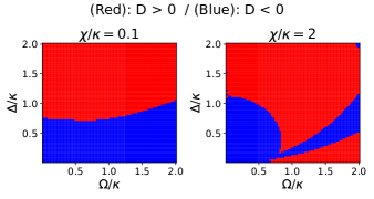
Figure 1: Parameter regions ensuring the Lindblad form of the time evolution generator $\mathcal{L}_{s}^{G=0}$ determined by the sign of $D$ (see Eq. (28)). The Lindblad form is attained in the red region $(D>0)$, while a dissipator comes with a negative cofficient in the blue region $(D<0)$. With the coupling strengths $(\chi_{1},\chi_{2},\chi_{3})=(0,\chi,2\chi)$, the left figure shows the result with $\chi/\kappa=0.1$ and the right figure with $\chi/\kappa=2$.

This example demonstrates that complete positivity (and positivity) of the partial trace evolution can be violated in adiabatic elimination, even without truncation in the expansion series. In this situation, the conjecture in Azouit17 states that the negative coefficient in front of a dissipator can be eliminated by a gauge transformation Eq. (12), and complete positivity of the reduced dynamics is restored in a different parametrization. In the current example, it is difficult to examine this conjecture for the following reason. Recall that the generator $\mathcal{L}_{s}^{G=0}$ given by Eq. (21) comprises of diagonal operators. Since there are only two linearly independent traceless operators when $d=3$ (see Eq. (26)), such a simple criterion as Eq. (28) can be obtained. However, the diagonal structure of the generator is lost when introducing a nontrivial gauge transformation. We then have eight linearly independent traceless operators, which preclude analytical studies of complete positivity.

IV Jaynes-Cummings model with damped oscillator

IV.1 Problem setting

To investigate roles of the gauge degree of freedom more closely, this section is dedicated to a slow qubit system being coupled to a strongly dissipative oscillator system. We assume that the Hamiltonian is given by the Jaynes-Cummings Hamiltonian and that the oscillator is coupled to a Markovian environment at finite temperature. The qubit is assumed to be non-dissipative for simplicity. In the frame rotating with the qubit frequency, we have

$$\mathcal{L}_{A}=-i\Delta_{A}(a^{\dagger}\!a)^{\times}+\gamma(1+n_{\rm th})\mathcal{D}[a]+\gamma n_{\rm th}\mathcal{D}[a^{\dagger}],$$ (29)

$$\epsilon\mathcal{L}_{\rm int}=-ig(a^{\dagger}\otimes\sigma_{-}+a\otimes\sigma_{+})^{\times},$$

and $\mathcal{L}_{B}=0$, with the oscillator detuning from the qubit frequency $\Delta_{A}$, the decay rate $\gamma$, the asymptotic oscillator quantum number in the absence of coupling $n_{\rm th}$ (see Eq. (57)), and the coupling constant $g$. $a$ and $a^{\dagger}$ are the annihilation and creation operators of the oscillator, respectively. This form of Lindbladian is used as a benchmark when analyzing oscillator-qubit interacting systems in cavity or superconducting circuit architecture.

The full spectrum and eigenoperators of $\mathcal{L}_{A}$ are provided in Appendix C. Result confirms, as long as $\gamma>0$, the existence of a unique steady state $\bar{\rho}_{A}$ given by Eq. (56).

IV.2 Fourth-order adiabatic elimination

To our knowledge, the invariance condition Eq. (3) for this system cannot be solved exactly. Thus, we perform the asymptotic expansion as discussed underneath Eq. (4). In this example, the timescale of the oscillator system is characterized by $\gamma^{-1}$, while that of the interaction is $|g|^{-1}$. Thus, the timescale separation parameter $\epsilon$ reads $\epsilon=|g|/\gamma$. Assuming $\epsilon\ll 1$, we calculate contributions up to the fourth-order.

As shown in Appendix C, $\mathcal{L}_{s}$ for the partial trace, $\mathcal{L}_{s}^{G=0}$, reads up to the fourth-order expansion

$$\begin{gathered}\mathcal{L}_{s}^{G=0}=-i\frac{\omega_{B}^{(4)}}{2}\sigma_{z}^{\times}\\ +\gamma_{-}^{(4)}\mathcal{D}[\sigma_{-}]+\gamma_{+}^{(4)}\mathcal{D}[\sigma_{+}]+\gamma_{\phi}^{(4)}\mathcal{D}[\sigma_{z}].\end{gathered}$$ (30)

The coefficients $\omega_{B}^{(4)}$, $\gamma_{\pm}^{(4)}$, and $\gamma_{\phi}^{(4)}$ are real numbers defined by

$$\omega_{B}^{(4)}={\rm Im}(b_{-}+b_{+}),\ \ \ \ \ \gamma_{\pm}^{(4)}=2{\rm Re}(b_{\pm}),$$

and

$$\gamma_{\phi}^{(4)}=-\frac{8g^{4}n_{+}n_{-}(3-6(2\Delta_{A}/\gamma)^{2}-(2\Delta_{A}/\gamma)^{4})}{\gamma^{3}(1+(2\Delta_{A}/\gamma)^{2})^{3}},$$

where $b_{\pm}$ are

$$b_{\pm}=\frac{2g^{2}n_{\pm}}{\bar{\gamma}}+\frac{8g^{4}n_{\pm}^{2}}{\bar{\gamma}^{3}}+\frac{8g^{4}n_{+}n_{-}(1+8i\gamma\Delta_{A}/|\bar{\gamma}|^{2})}{\bar{\gamma}^{*}|\bar{\gamma}|^{2}},$$

with $n_{+}=n_{\rm th}$, $n_{-}=1+n_{\rm th}$, and $\bar{\gamma}=\gamma+2i\Delta_{A}$.

The coefficient $\omega_{B}^{(4)}$ represents the qubit frequency shift due to the coupling with the oscillator. Up to the second-order, $\omega_{B}^{(2)}$, it reads $\omega_{B}^{(2)}=-4\Delta_{A}g^{2}(n_{-}+n_{+})/|\bar{\gamma}|^{2}$. The $\gamma_{\pm}^{(4)}$ and $\gamma_{\phi}^{(4)}$ terms describe the effective qubit decay induced by the coupling to the dissipative oscillator. On the one hand, when $|g|/\gamma\ll 1$, $\gamma_{\pm}^{(4)}$ are dominated by the second-order contributions given by $\gamma_{\pm}^{(2)}=4g^{2}\gamma n_{\pm}/|\bar{\gamma}|^{2}>0$, and thus $\gamma_{\pm}^{(4)}>0$. On the other hand, $\gamma_{\phi}^{(4)}$ involves only the fourth-order contribution and

$$\begin{gathered}\gamma_{\phi}^{(4)}<0\ \ \ {\rm when}\\ n_{\rm th}>0\ \ {\rm and}\ \ |\Delta_{A}|/\gamma<\sqrt{2\sqrt{3}-3}/2\simeq 0.34,\end{gathered}$$ (31)

even if the condition for the asymptotic expansion, $|g|/\gamma\ll 1$, holds.

The stability of the time evolution when $\gamma_{\phi}^{(4)}<0$ can be confirmed by calculating the eigenvalues of $\mathcal{L}_{s}^{G=0}$ as follows. With $I_{B}$ the identity matrix on $\mathscr{H}_{B}$ ($2$-dimensional identity matrix), the set $\{I_{B}/\sqrt{2},\sigma_{x}/\sqrt{2},\sigma_{y}/\sqrt{2},\sigma_{z}/\sqrt{2}\}$ is an orthonormal basis with the Hilbert-Schmidt inner product. Let $[\mathcal{L}_{s}^{G=0}]$ be the $4\times 4$ matrix representation of $\mathcal{L}_{s}^{G=0}$ in this basis. It reads

$$[\mathcal{L}_{s}^{G=0}]=\begin{pmatrix}0&0&0&0\\ 0&-1/T_{2}&-\omega_{B}^{(4)}&0\\ 0&\omega_{B}^{(4)}&-1/T_{2}&0\\ R_{z}/T_{1}&0&0&-1/T_{1}\end{pmatrix},$$

with $1/T_{1}=\gamma_{-}^{(4)}+\gamma_{+}^{(4)}$, $1/T_{2}=1/(2T_{1})+2\gamma_{\phi}^{(4)}$, and $R_{z}=-(\gamma_{-}^{(4)}-\gamma_{+}^{(4)})T_{1}$. From this, the spectrum of $\mathcal{L}_{s}^{G=0}$ is given by $\{0,-1/T_{2}+i\omega_{B}^{(4)},-1/T_{2}-i\omega_{B}^{(4)},-1/T_{1}\}$. By multiplying $t$ and then exponentiating them, we obtain the spectrum of the time evolution map $\exp(\mathcal{L}_{s}^{G=0}t)$,

$$\{1,e^{-t/T_{2}+i\omega_{B}^{(4)}t},e^{-t/T_{2}-i\omega_{B}^{(4)}t},e^{-t/T_{1}}\}.$$ (32)

Since $\gamma_{\pm}^{(4)}>0$ and $\gamma_{\pm}^{(4)}\gg|\gamma_{\phi}^{(4)}|$ when $|g|/\gamma$ is small, we have $T_{1}>0$ and $T_{2}>0$. Therefore, the time evolution is stable even when $\gamma_{\phi}^{(4)}$ is negative.

Note that $\sigma_{\pm}$ and $\sigma_{z}$ are linearly independent and traceless. When $\gamma_{\phi}^{(4)}$ is negative, thus, $\mathcal{L}_{s}^{G=0}$ is not a Lindbladian from Corollary 1 in Appendix A.

Unlike the example in the previous section, on the other hand, the time evolution map is positive even when $\gamma_{\phi}^{(4)}<0$. To see this, we introduce the Bloch vector $\bm{r}(t)=(r_{x}(t),r_{y}(t),r_{z}(t))^{\top}\in\mathbb{R}^{3}$, which is related to the partial trace as $\rho_{B}(t)=(I_{B}+\sum_{i=x,y,z}r_{i}(t)\sigma_{i})/2$. From Eq. (30), the evolution of the Bloch vector reads

$$\begin{gathered}\frac{d}{dt}r_{x}(t)=-\frac{r_{x}(t)}{T_{2}}-\omega_{B}^{(4)}r_{y}(t),\\ \frac{d}{dt}r_{y}(t)=-\frac{r_{y}(t)}{T_{2}}+\omega_{B}^{(4)}r_{x}(t),\\ \frac{d}{dt}r_{z}(t)=-\frac{1}{T_{1}}(r_{z}(t)-R_{z}).\end{gathered}$$

These equations mean that that $R_{z}$ is the asymptotic value of $r_{z}(t)$, $\lim_{t\to\infty}\bm{r}(t)=(0,0,R_{z})^{\top}$. They also lead to

$$\frac{d}{dt}\bm{r}^{2}(t)=-2\Big{(}\frac{\bm{r}^{2}(t)-r_{z}^{2}(t)}{T_{2}}+\frac{r_{z}(t)(r_{z}(t)-R_{z})}{T_{1}}\Big{)}.$$

The partial trace $\rho_{B}(t)$ is positive semidefinite if and only if $\bm{r}^{2}(t)\leq 1$. If we have $(d/dt)\bm{r}^{2}(t)<0$ under the constraint $\bm{r}^{2}(t)=1$ for any $t$, then $\bm{r}^{2}(t)$ does not exceed unity along the time evolution and thus positivity is preserved. Substituting $\bm{r}^{2}(t)=1$ into the above equation, we obtain

$$\begin{gathered}\frac{d}{dt}\bm{r}^{2}(t)=\\ -\frac{2}{\Delta T}\Big{[}\Big{(}r_{z}(t)-\frac{\Delta T}{2T_{1}}R_{z}\Big{)}^{2}+(\Delta T)^{2}(\gamma_{-}^{(4)}\gamma_{+}^{(4)}-4(\gamma_{\phi}^{(4)})^{2})\Big{]},\end{gathered}$$

with $1/\Delta T=1/T_{1}-1/T_{2}=(\gamma_{-}^{(4)}+\gamma_{+}^{(4)})/2-2\gamma_{\phi}^{(4)}$. When $|g|/\gamma\ll 1$, we have $\gamma_{\pm}^{(4)}\gg|\gamma_{\phi}^{(4)}|$. This leads to $\Delta T>0$ and $\gamma_{-}^{(4)}\gamma_{+}^{(4)}>4(\gamma_{\phi}^{(4)})^{2}$. Therefore, $(d/dt)\bm{r}^{2}(t)<0$ whenever $\bm{r}^{2}(t)=1$. This proves that the time evolution map is positive even with a negative value of $\gamma_{\phi}^{(4)}$.

This mechanism appears to be related to the well-known example of the transpose of a matrix, which is positive but not complete positivity. Indeed, that standard example essentially says that an evolution which contracts a single Bloch vector direction fast, but the two other directions slowly, is not completely positive. We here have this situation with $\gamma_{\phi}<0$ slowing down the contraction of $r_{x}$ and $r_{y}$.

IV.3 Gauge transformation

When $\gamma_{\phi}^{(4)}<0$, $\mathcal{L}_{s}^{G=0}$ is not a Lindbladian. To be more precise, the time evolution map with $\mathcal{L}_{s}^{G=0}$ is not completely positive. On the other hand, the Lindblad form might be recovered in another gauge choice, as conjectured in Azouit17 . In this subsection, however, we prove that this is impossible. As shown in Eq. (12), the gauge transformation induces similarity transformation. To our knowledge, similarity transformation of the time evolution generator has not been discussed extensively in the literature. To demonstrate its role, therefore, we first consider the following toy example. Suppose a time evolution equation $(d/dt)\rho=\mathcal{L}_{0}(\rho)$ with

$$\mathcal{L}_{0}=-i\frac{\omega_{0}}{2}\sigma_{z}^{\times}+\gamma_{0}\mathcal{D}[\sigma_{x}]-\gamma_{0}\mathcal{D}[\sigma_{y}],$$

where $\omega_{0}$ and $\gamma_{0}$ are real and positive parameters. To ensure the stability of the evolution, we assume $\omega_{0}>2\gamma_{0}$. Since $\sigma_{x}$ and $\sigma_{y}$ are linearly independent and traceless, the negative sign in front of $\mathcal{D}[\sigma_{y}]$ means that $\mathcal{L}_{0}$ is not a Lindbladian. This negativity can be removed by the similarity transformation

$$\mathcal{L}_{0}^{\prime}=e^{-q_{0}\mathcal{D}[\sigma_{x}+\sigma_{y}]}\circ\mathcal{L}_{0}\circ e^{q_{0}\mathcal{D}[\sigma_{x}+\sigma_{y}]},$$

with $q_{0}$ defined by $\tanh(4q_{0})=2\gamma_{0}/\omega_{0}$ because $\mathcal{L}_{0}^{\prime}$ reads

$$\mathcal{L}_{0}^{\prime}=-i\frac{\omega_{0}^{\prime}}{2}\sigma_{z}^{\times},$$

with $\omega_{0}^{\prime}=\sqrt{\omega_{0}^{2}-4\gamma_{0}^{2}}$. As a result, the above similarity transformation restores the Lindblad form.

Since $\mathcal{L}_{0}$ and $\mathcal{L}_{0}^{\prime}$ have the same spectrum, so do the time evolution maps $\exp(\mathcal{L}_{0}t)$ and $\exp(\mathcal{L}_{0}^{\prime}t)$. At infinitesimal $t$, $\exp(\mathcal{L}_{0}^{\prime}t)$ is a Kraus map, while $\exp(\mathcal{L}_{0}t)$ is not. Thus, this example shows that one cannot judge only from the spectrum whether the map is a Kraus map or not. On the other hand, in this example, one can anticipate the existence of a Kraus map which has the same spectrum as $\exp(\mathcal{L}_{0}t)$. Note that the spectrum of $\exp(\mathcal{L}_{0}t)$ is given by $\{1,1,\exp(i\omega_{0}^{\prime}t),\exp(-i\omega_{0}^{\prime}t)\}$. This implies that the time evolution merely induces a rotation of the Bloch vector without damping, which then implies that the evolution can be described by a unitary transformation or a Kraus map in a suitable basis. In fact, this argument can be generalized at least for qubit maps. That is, for a given set of four numbers, $\Lambda\in\mathbb{C}^{4}$, one can discuss the existence of a Kraus map whose spectrum is given by $\Lambda$. This is guaranteed by Theorem 1 of WPG10 which states the following;

Theorem (M. M. Wolf and D. Perez-Garcia).

Given $\Lambda\in\mathbb{C}^{4}$, the following statements are equivalent:

• There exists a Kraus map the spectrum of which is given by $\Lambda$.

• $\Lambda={1}\cup\lambda$ where $\lambda\in\mathbb{C}^{3}$ is closed under complex conjugation. Furthermore, if we define $s\in\mathbb{R}^{3}$ by $s_{i}=\lambda_{i}$ if $\lambda_{i}\in\mathbb{R}$ and $s_{i}=|\lambda_{i}|$ otherwise, then

  $$s\in\mathcal{T},$$ (33)

  where $\mathcal{T}\subset\mathbb{R}^{3}$ is the tetrahedron whose corners are $(1,1,1)$, $(1,-1,-1)$, $(-1,1,-1)$, and $(-1,-1,1)$.

With this theorem, we consider $\mathcal{L}_{s}^{G=0}$ in Eq. (30). Let $\Lambda$ be the spectrum of the time evolution map $\exp(\mathcal{L}_{s}^{G=0}t)$. From Eq. (32), we set

$$\Lambda=\{1,e^{-t/T_{2}+i\omega_{B}^{(4)}t},e^{-t/T_{2}-i\omega_{B}^{(4)}t},e^{-t/T_{1}}\}.$$

$\Lambda$ is closed under complex conjugation. From the definition, $\{s_{i}\}$ are now all positive. In this case, assuming $s_{1}\geq s_{2}\geq s_{3}$, the condition Eq. (33) reads $s_{1}\leq 1$ and $s_{1}+s_{2}\leq 1+s_{3}$ (see WPG10 ). When $\gamma_{\phi}^{(4)}<0$, we always have $1/T_{1}>1/T_{2}$, and $\exp(-t/T_{2})>\exp(-t/T_{1})$ for $t>0$. Thus, we set $s_{1}=s_{2}=\exp(-t/T_{2})$ and $s_{3}=\exp(-t/T_{1})$. Then, while the first condition $s_{1}\leq 1$ is satisfied, the second condition reads

$$2e^{-t/T_{2}}\leq 1+e^{-t/T_{1}}.$$ (34)

For an infinitesimal time $t$ such that $\exp(-t/T_{i})\simeq 1-t/T_{i}\ (i=1,2)$, this condition reads $\gamma_{\phi}^{(4)}\geq 0$ and is violated if $\gamma_{\phi}^{(4)}<0$. Therefore, there does not exist a Kraus map which has the same spectrum as $\exp(\mathcal{L}_{s}^{G=0}t)$ at least at infinitesimal times $t$. From Eq. (12), the gauge transformation induces similarity transformation of the time evolution map,

$$e^{\mathcal{L}_{s}^{G}t}=(\mathcal{I}_{B}+G)^{-1}\circ e^{\mathcal{L}_{s}^{G=0}t}\circ(\mathcal{I}_{B}+G).$$

This proves that $\exp(\mathcal{L}_{s}^{G}t)$ at infinitesimal times $t$ is not a Kraus map in any choice of gauge $G$.

In conclusion of this section, the oscillator-qubit system discussed here serves as a counterexample to the conjecture in Azouit17 .

V Discussion

In this section, we discuss interpretation of the results found so far. First, we focus our attention on the origin of the negative coefficient observed in the generator for the partial trace evolution. We then make several remarks on roles of the gauge degree of freedom. We have seen that it is the violation of complete positivity that causes a non-Lindblad form of the generator. In the formulation presented in Sec. II, this is generally the case for the partial trace $\mathcal{L}_{s}^{G=0}$ (and also for any gauge choice as long as the gauge superoperator $G$ preserves the Hermitian property and trace). The generator is given by a Lindbladian if and only if the time evolution map satisfies the semigroup relation and is a Kraus map. The semigroup relation is guaranteed because the slow dynamics is restricted on an invariant manifold exactly. The Hermitian and trace preservations are also satisfied generally. This can be seen from the definition of $\mathcal{L}_{s}^{G=0}$ (see Eq. (7)) together with the fact that $\mathcal{L}_{A}^{+}$ is a Hermitian and trace preserving map (see Eq. (47)). Complete positivity, however, is a nontrivial condition and it can be violated as we have seen in the previous sections. We recall that not only complete positivity but even positivity of the time evolution map can be violated as shown with the qudit-qubit example in Sec. III. In this case, the density matrix acquires a negative eigenvalue depending on the initial state, and thus the result cannot be interpreted physically.

In addition, we stress that the complete positivity violation is not an artifact caused by truncating the series expansion at a finite order. With the qubit-qutrit example presented in Sec. III, we have seen that the negative coefficient in front of a dissipator appears even in all-order analysis. For the oscillator-qubit example in Sec. IV, contributions higher than the fourth-order only correct the values of $1/T_{1}$ and $1/T_{2}$ in Eq. (34). Thus, for small enough $|g|/\gamma$, they cannot cure the violation of the inequality at the fourth-order.

In order to understand the origin of a non-Lindblad form, let us recall the reason why we expected a completely positive evolution in the first place. To this end, we write the time evolution of the partial trace via that of the total state. If we assume a separable initial state with $\bar{\rho}_{A}$, we have

$$\rho_{B}(t)={\rm tr}_{A}\circ e^{\mathcal{L}_{\rm tot}t}(\bar{\rho}_{A}\otimes\rho_{B}(t=0)).$$ (35)

Note that ${\rm tr}_{A}$, $\exp(\mathcal{L}_{\rm tot}t)$, and the map that sends $\rho_{B}(t=0)$ to $\bar{\rho}_{A}\otimes\rho_{B}(t=0)$ are all completely positive. Therefore, the time evolution map from an initial state $\rho_{B}(t=0)$ to $\rho_{B}(t)$ is completely positive.

Here, it should be recalled that, in adiabatic elimination, we initialize a state on an invariant manifold. When $\epsilon=0$, a set of density matrices on the invariant manifold is characterized by separable states as $\mathcal{K}_{0}^{G=0}(\rho_{B})=\bar{\rho}_{A}\otimes\rho_{B}$ (see Eq. (5)). In this case, Eq. (35) describes the slow dynamics on the invariant manifold, where $\bar{\rho}_{A}$ is fixed. When $\epsilon>0$, however, the slow manifold is not anymore of the form $\{\bar{\rho}_{A}\otimes\rho_{B}\}$ , so the initial state of Eq. (35) does not lie on the invariant manifold, and Eq. (35) includes the transient dynamics of the fast degrees of freedom. Long after decay time of the fast sub-system, say $t\geq t_{\rm inv}$, the total state $\rho(t)$ is approximately on an invariant manifold. In this situation, the time evolution map calculated in adiabatic elimination is the one that sends $\rho_{B}(t_{\rm inv})={\rm tr}_{A}(\rho(t_{\rm inv}))$ to $\rho_{B}(t)\ (t\geq t_{\rm inv})$. There is no guarantee that this map is completely positive, even though the map that sends $\rho_{B}(t=0)$ to $\rho_{B}(t)$ is completely positive. This situation is illustrated in Fig. 2.

Figure 2: Schematic illustration of the total state evolution with an initial separable state. On the grayish planes showing invariant manifolds with vanishing and a non-zero value of $\epsilon$, the reddish areas show a set of density matrices. As shown by the green arrow, the trajectory starting from a separable state is first attracted to the invariant manifold with $\epsilon>0$ (the darker grayish plane) and then is restricted on there for $t\geq t_{\rm inv}$ (the slow dynamics). While complete positivity is ensured for the partial trace evolution including the attracting phase ($\rho_{B}(t=0)\to\rho_{B}(t)$), it is not always the case for the slow dynamics ($\rho_{B}(t_{\rm inv})\to\rho_{B}(t)$).

In the transient regime, a master equation for the partial trace depends explicitly on time owing to the evolution of the fast degrees of freedom. After relaxation of them, we obtain a time-independent master equation, and that is what we calculate in adiabatic elimination. In this view, we note a similarity to non-positivity in the Redfield equation, which is derived by making the Born-Markov approximation to a system-environment Hamiltonian under the condition of an initial separable state Breuer02 . The Redfield equation with the asymptotic time-independent coefficient violates (complete) positivity. On the other hand, positivity is restored by taking into account time-dependence of the coefficient as shown in Whitney08 ; Hartmann20 . The same should hold true in the composite Lindblad systems discussed in this paper. In Appendix D, this expectation is confirmed for the qudit system in Sec. III by calculating the exact master equation for the partial trace with a separable initial state. While the analytic structure of the complete positivity violation is similar between higher-order adiabatic elimination and the Redfield equation, the geometric picture is not applicable to the latter. We will discuss below that it provides us with a clear interpretation of the non-positive evolution.

To account for the initialization on the invariant manifold, Eq. (35) should be rewritten as

$$\rho_{B}(t)={\rm tr}_{A}\circ e^{\mathcal{L}_{\rm tot}t}\circ\mathcal{K}^{G=0}(\rho_{B}(t=0)).$$ (36)

From this equation and complete positivity of ${\rm tr}_{A}$ and $e^{\mathcal{L}_{\rm tot}t}$, the complete positivity violation of the time evolution map stems from that of $\mathcal{K}^{G=0}$. In what follows, we investigate properties of $\mathcal{K}^{G=0}$. We first focus on the oscillator-qubit system and then generalize the obtained results.

For the oscillator-qubit system, let us assume $\Delta_{A}=0$ for simplicity. Then, the expansion up to the second-order of $g/\gamma$ reads (see Appendix E)

$$\begin{gathered}\mathcal{K}^{G=0}(\rho_{B})=W(\bar{\rho}_{A}\otimes\rho_{B})W^{\dagger}\\ -\Big{[}\frac{4g^{2}(1+n_{\rm th})}{\gamma^{2}}(I_{A}\otimes\sigma_{-})(\bar{\rho}_{A}\otimes\rho_{B})(I_{A}\otimes\sigma_{-})^{\dagger}\\ +\frac{4g^{2}n_{\rm th}}{\gamma^{2}}(I_{A}\otimes\sigma_{+})(\bar{\rho}_{A}\otimes\rho_{B})(I_{A}\otimes\sigma_{+})^{\dagger}\Big{]},\end{gathered}$$ (37)

with $I_{A}$ the identity operator on $\mathscr{H}_{A}$ and $W=I_{A}\otimes I_{B}-(2ig/\gamma)(a^{\dagger}\otimes\sigma_{-}+a\otimes\sigma_{+})-(2g^{2}/\gamma^{2})(a^{\dagger}\!a-n_{\rm th}I_{A})\otimes I_{B}$.

Because of the minus signs in the last two lines, the second-order expansion of $\mathcal{K}^{G=0}$ is not completely positive. From the construction, $\mathcal{L}^{G=0}_{s,n}$ with a positive integer $n$ depends on $\{\mathcal{K}^{G=0}_{k}\}_{k=0,1,\dots,n-1}$. For the oscillator-qubit system, we have $\mathcal{L}^{G=0}_{s,2n-1}=0$. Thus, complete positivity of the time evolution map can be violated from the fourth-order expansion. This consideration is consistent with the result in Sec. IV. It should be noted that the time evolution map can be completely positive even if $\mathcal{K}^{G=0}$ is not. If $n_{\rm th}=0$, for instance, $\gamma_{\phi}^{(4)}=0$ and the generator $\mathcal{L}_{s}^{G=0}$ is in the Lindblad form up to the fourth-order terms, despite that $\mathcal{K}^{G=0}$ still contains a negative term.

Strikingly, $\mathcal{K}^{G=0}$ in Eq. (37) is not even positive. To see this, let $\ket{0}\in\mathscr{H}_{A}$ be the vacuum state of the oscillator and $\ket{\psi}\in\mathscr{H}_{B}$ be a state. The matrix element of $\mathcal{K}^{G=0}$ with respect to $\ket{0,\psi}=\ket{0}\otimes\ket{\psi}$ reads

$$\begin{gathered}\braket{0,\psi}{\mathcal{K}^{G=0}(\rho_{B})}{0,\psi}=\braket{0}{\bar{\rho}_{A}}{0}\Big{[}\Big{(}1+\frac{4g^{2}n_{\rm th}}{\gamma^{2}}\Big{)}\braket{\psi}{\rho_{B}}{\psi}\\ -\frac{4g^{2}(1+n_{\rm th})}{\gamma^{2}}\,\braket{\psi_{+}}{\rho_{B}}{\psi_{+}}-\frac{4g^{2}n_{\rm th}^{2}}{\gamma^{2}(1+n_{\rm th})}\,\braket{\psi_{-}}{\rho_{B}}{\psi_{-}}\Big{]}.\end{gathered}$$

with $\ket{\psi_{\pm}}=\sigma_{\pm}\ket{\psi}$. If $\rho_{B}$ is a pure state, its kernel is not empty. Suppose $\ket{\psi}$ is in the kernel of $\rho_{B}$, that is, $\rho_{B}\ket{\psi}=0$. Since either $\braket{\psi_{+}}{\rho_{B}}{\psi_{+}}$ or $\braket{\psi_{-}}{\rho_{B}}{\psi_{-}}$ is non-zero, we obtain $\braket{0,\psi}{\mathcal{K}^{G=0}(\rho_{B})}{0,\psi}<0$. Consequently, $\mathcal{K}^{G=0}$ is not positive, let alone completely positive.

To clarify the situation, we introduce the following symbols for general settings; let $\mathscr{M}_{\rm inv}$ be a set of density matrices on an invariant manifold and $\mathscr{D}(\mathscr{H})$ be a set of density matrices on a Hilbert space $\mathscr{H}$. The assignment map is $\mathcal{K}^{G=0}:\mathscr{D}(\mathscr{H}_{B})\to\mathscr{M}_{\rm inv}$ and, conversely, the partial trace operation ${\rm tr}_{A}$ can be seen as a map ${\rm tr}_{A}:\mathscr{M}_{\rm inv}\to\mathscr{D}(\mathscr{H}_{B})$. We first note that, for every $\rho^{*}\in\mathscr{M}_{\rm inv}$, its partial trace is a density matrix, $\rho_{B}^{*}\equiv{\rm tr}_{A}(\rho^{*})\in\mathscr{D}(\mathscr{H}_{B})$, and we have $\rho^{*}=\mathcal{K}^{G=0}(\rho_{B}^{*})$ by the construction of $\mathcal{K}^{G=0}$. In addition to this, we have seen for the oscillator-qubit system that the second-order expansion of $\mathcal{K}^{G=0}$ is not positive. These imply $\mathscr{M}_{\rm inv}\subset\mathcal{K}^{G=0}(\mathscr{D}(\mathscr{H}_{B}))$. Similarly, while the partial trace map is injective from ${\rm tr}_{A}\circ\mathcal{K}^{G=0}=\mathcal{I}_{B}$ and the uniqueness of $\mathcal{K}^{G=0}$, it is not surjective because, for the oscillator-qubit system, any pure density matrix on $\mathscr{H}_{B}$ cannot be obtained by taking the partial trace of states in $\mathscr{M}_{\rm inv}$. In other words, we have ${\rm tr}_{A}(\mathscr{M}_{\rm inv})\subset\mathscr{D}(\mathscr{H}_{B})$. Therefore, the situation can be illustrated as in Fig. 3.

Figure 3: Schematic illustration of the non-surjective property of the partial trace map ${\rm tr}_{A}$ and the positivity violation of $\mathcal{K}^{G=0}$ for the oscillator-qubit system. Density matrices on the invariant manifold $\mathscr{M}_{\rm inv}$ shown by the reddish area are entangled states when $\epsilon>0$. As a result, the partial trace of that set ${\rm tr}_{A}(\mathscr{M}_{\rm inv})$ becomes a subset, shown by the reddish spheroid, of the Bloch sphere $\mathscr{D}(\mathscr{H}_{B})$. Conversely, assignment of the whole Bloch sphere $\mathcal{K}^{G=0}(\mathscr{D}(\mathscr{H}_{B}))$ results in a larger set, enclosed by the dashed line on the invariant manifold, than $\mathscr{M}_{\rm inv}$.

The positivity violation of $\mathcal{K}^{G=0}$ (the non-surjective property of the partial trace map) can be understood from the correlation between the two sub-systems as discussed for Hamiltonian systems in CPdebate . When $\epsilon=0$, states in $\mathscr{M}_{\rm inv}$ are characterized by $\bar{\rho}_{A}\otimes\rho_{B}$ as mentioned above. For these non-interacting separable states, any reduced state $\rho_{B}$ can be assigned to a valid total state. When $\epsilon>0$, on the other hand, states in $\mathscr{M}_{\rm inv}$ are no longer separable due to the interaction term. At the second-order of $\epsilon$, they include entangled states in general. Then, there exist pure reduced states that cannot be assigned to any valid total state.

The aforementioned picture holds true in a general class of settings, not only for the oscillator-qubit system. As shown in Theorem 6 of AzouitThesis (see Appendix E), while there always exist gauge choices such that $\mathcal{K}^{G}$ is completely positive up to the second-order expansion, in general $\mathcal{K}^{G=0}$ is not. Furthermore, we can show the positivity violation of $\mathcal{K}^{G=0}$ (the non-surjective property of the partial trace map) in the following way. We first note a theorem regarding assignment maps, which was first proved for qubit reduced systems in CPdebate and later generalized in Jordan04 . Let $\Phi:\mathscr{D}(\mathscr{H}_{B})\to\mathscr{D}(\mathscr{H}_{A}\otimes\mathscr{H}_{B})$ be a map assigning a reduced state in $\mathscr{H}_{B}$ a total state in $\mathscr{D}(\mathscr{H}_{A}\otimes\mathscr{H}_{B})$. Then, the following statements are equivalent;

• $\Phi$ is linear, consistent (${\rm tr}_{A}\circ\Phi=\mathcal{I}_{B}$), and positive ($\Phi(\rho_{B})\in\mathscr{D}(\mathscr{H}_{A}\otimes\mathscr{H}_{B})$ for every $\rho_{B}\in\mathscr{D}(\mathscr{H}_{B})$).

• For every $\rho_{B}\in\mathscr{D}(\mathscr{H}_{B})$, $\Phi(\rho_{B})=\rho_{A}\otimes\rho_{B}$ where $\rho_{A}\in\mathscr{D}(\mathscr{H}_{A})$ is independent of $\rho_{B}$.

We now apply this theorem to the assignment map in adiabatic elimination, $\mathcal{K}^{G=0}$. Since it is linear and consistent, $\mathcal{K}^{G=0}$ is positive if and only if $\mathscr{M}_{\rm inv}$ is characterized by separable states with a fixed state on $\mathscr{D}(\mathscr{H}_{A})$. Due to the interaction term, $\mathscr{M}_{\rm inv}$ at the second-order expansion includes entangled states in general. Therefore, the corresponding $\mathcal{K}^{G=0}$ is non-positive. One might argue that non-separable states should also be obtained in the first-order expansion of $\epsilon$. On this point, we note that the first-order expansion of $\mathcal{K}^{G=0}$ reads (see Eq. (66))

$$\begin{gathered}\mathcal{K}^{G=0}(\rho_{B})=\\ \bar{\rho}_{A}\otimes\rho_{B}-i\epsilon(M(\bar{\rho}_{A}\otimes\rho_{B})-(\bar{\rho}_{A}\otimes\rho_{B})M^{\dagger}),\end{gathered}$$ (38)

where $M$ satisfies ${\rm tr}_{A}(M\bar{\rho}_{A})=0$. In agreement with the above theorem, this is not positive. We here note that this can be rewritten as

$$\begin{gathered}\mathcal{K}^{G=0}(\rho_{B})=\\ (I_{A}\otimes I_{B}-i\epsilon M)(\bar{\rho}_{A}\otimes\rho_{B})(I_{A}\otimes I_{B}-i\epsilon M)^{\dagger}\\ -\epsilon^{2}M(\bar{\rho}_{A}\otimes\rho_{B})M^{\dagger}.\end{gathered}$$ (39)

Within the accuracy of the first-order expansion, we can neglect the third line and obtain a Kraus map form of $\mathcal{K}^{G=0}$. Since the neglect of the third line violates the consistency at order $\epsilon^{2}$, this result does not contradict with the above theorem either. In the second-order expansion, on the other hand, there is a negative term that cannot be eliminated within that accuracy. This results in the positivity violation of $\mathcal{K}^{G=0}$.

While the map $\mathcal{K}^{G=0}$ resulting from the first-order expansion, i.e. Eq. (38), is not completely positive, its rewriting with Eq. (39) shows that the non-positivity only yields a term of order $\epsilon^{2}$. This explains the reason why the Lindblad form must always be obtained including the second-order contribution, as shown in Azouit17 . The non-positivity of $\mathcal{K}^{G=0}$ at second-order indicates danger for the third-order expansion and higher. For the oscillator-qubit system, the third-order contribution $\mathcal{L}_{s,3}^{G=0}$ vanishes and the non-Lindblad form is obtained from the fourth-order expansion. Even when $\mathcal{L}_{s,3}^{G=0}$ does not vanish, it was shown in Theorem 9 of AzouitThesis that, if the interaction Hamiltonian is separable and the second-order contribution does not vanish, $\mathcal{L}_{s}^{G=0}$ admits the Lindblad form up to the third-order expansion. The extension of this result to a general interaction Hamiltonian is discussed in Appendix E. These result from the fact that the third-order contribution can be absorbed to the second-order contribution which is in the Lindblad form in general.

So far we have concentrated on the parametrization via the partial trace. Now let us consider how the gauge degree of freedom plays its role in the above discussion. While the second-order expansion of $\mathcal{K}^{G=0}$ is not completely positive, there always exist gauge choices $G$ such that $\mathcal{K}^{G}$ has that property. This was proved in Theorem 6 of AzouitThesis and the calculation is repeated in Appendix E. Note that this does not contradict with the theorem regarding assignment maps presented above Eq. (38), since, when $G\neq 0$, the map $\mathcal{K}^{G}$ is not consistent as ${\rm tr}_{A}\circ\mathcal{K}^{G}=\mathcal{I}_{B}+G$. The gauge choices restoring complete positivity of the assignment is obtained in Eq. (68). For the oscillator-qubit system, one choice (setting $z=1$ in Eq. (68)) reads

$$G(\rho_{s})=\frac{4g^{2}(1+n_{\rm th})}{\gamma^{2}}\mathcal{D}[\sigma_{-}](\rho_{s})+\frac{4g^{2}n_{\rm th}}{\gamma^{2}}\mathcal{D}[\sigma_{+}](\rho_{s}),$$

and $\mathcal{K}^{G}$ up to the second-order expansion is given by

$$\mathcal{K}^{G}(\rho_{s})=W(\bar{\rho}_{A}\otimes\rho_{s})W^{\dagger},$$

where $W$ was introduced in Eq. (37).

Even when $\mathcal{K}^{G}$ is completely positive, however, the Lindblad form of the generator $\mathcal{L}_{s}^{G}$ is not guaranteed. As in Eq. (36), we have

$$\rho_{B}(t)={\rm tr}_{A}\circ e^{\mathcal{L}_{\rm tot}t}\circ\mathcal{K}^{G}(\rho_{s}(0)).$$

Note that the map $\Upsilon_{t}^{G}={\rm tr}_{A}\circ e^{\mathcal{L}_{\rm tot}t}\circ\mathcal{K}^{G}$ is completely positive, but now its input is not $\rho_{B}(0)$ anymore. To recover a semi-group starting at identity of the form $\exp(\mathcal{L}_{s}^{G}t)$, we must either map $\rho_{s}(0)$ to $\rho_{B}(0)$, or map $\rho_{B}(t)$ to $\rho_{s}(t)$. The conclusions will be similar, so let us consider the evolution of $\rho_{s}$ by using $\rho_{s}(t)=(\mathcal{I}_{B}+G)^{-1}(\rho_{B}(t))$;

$$\rho_{s}(t)=(\mathcal{I}_{B}+G)^{-1}\circ\Upsilon_{t}^{G}(\rho_{s}(0)).$$ (40)

When $\mathcal{K}^{G}$ is completely positive, so is $(\mathcal{I}_{B}+G)$. Therefore, $(\mathcal{I}_{B}+G)^{-1}$ is not completely positive in general, neither is the time evolution map for $\rho_{s}$, i.e. $(\mathcal{I}_{B}+G)^{-1}\circ\Upsilon_{t}^{G}$. We have seen above that the complete positivity violation of the partial trace evolution is a natural consequence of quantum entanglement and Eq. (36). On the other hand, we cannot judge from Eq. (40) whether it is possible to restore complete positivity or not. This underlines the importance of the analysis in Sec. IV

In practical applications, care should be taken if the initial state is determined in the reduced system. For the partial trace parametrization, the domain of initial reduced states must be restricted to ${\rm tr}_{A}(\mathscr{M}_{\rm inv})$, which is a subset of $\mathscr{D}(\mathscr{H}_{B})$ in general. By linearity, extending the domain of $\mathcal{K}^{G=0}$ to $\mathscr{D}(\mathscr{H}_{B})$ (all density matrices) is possible. However, such extension leads to an initial total state that is not positive semidefinite and thus is unphysical. Recall that $\mathcal{K}^{G=0}$ is not positive at the second-order expansion in general. Therefore, the domain restriction is necessary once we consider contributions higher than the second-order, even when $\mathcal{L}_{s}^{G=0}$ admits the Lindblad form.

In order to simulate all the possible dynamics on $\mathscr{M}_{\rm inv}$ via the reduced model, the map $\mathcal{K}^{G}:\mathscr{D}(\mathscr{H}_{B})\to\mathscr{M}_{\rm inv}$ needs to be positive and surjective. If $G=G_{ps}$ has those properties, then the time evolution map with this gauge choice $\exp(\mathcal{L}_{s}^{G_{ps}}t)$ at least preserves positivity. Indeed, since $\mathcal{K}^{G_{ps}}$ maps $\mathscr{D}(\mathscr{H}_{B})$ onto all the positive states in the subspace spanned by $\mathscr{M}_{\rm inv}$, by injectivity a non-positive $\rho_{s}$ obtained with $\exp(\mathcal{L}_{s}^{G_{ps}}t)$ can also be mapped only onto a non-positive $\rho$ in the space spanned by $\mathscr{M}_{\rm inv}$.

Contrary to the conjecture in Azouit17 , we do not believe that such a $G_{ps}$ exists in general. To our knowledge, the existence of $G_{ps}$ has been confirmed only for a dispersively coupled two qubit system in Alain20 . The approach employed to prove this result is not applicable to the dispersive qubit-qutrit system, as discussed in Appendix F.

VI Concluding remarks

Higher-order adiabatic elimination (higher than the second-order) can lead to the slow evolution of the partial trace that is not completely positive. This is due to the fact that states on an invariant manifold include correlation between the fast and slow sub-systems, which imposes a restriction on the domain of proper reduced states. Although the existence of a gauge choice restoring complete positivity was conjectured, we have shown that it is not the case for the oscillator-qubit system discussed in Sec. IV.

On experimental side, the fact that higher-order reduced model (for the partial trace) can potentially lead to unphysical results such as negative population can be understood as follows. As we have emphasized throughout the paper, adiabatic elimination describes slow dynamics on an invariant manifold. It is unlikely that a prepared initial state in an experimental setting is exactly on an invariant manifold. As an easily imaginable setting, suppose that two sub-systems have been evolved independently and an interaction is switched on abruptly at $t=0$. The initial state is then given by $\rho(t=0)=\bar{\rho}_{A}\otimes\rho_{B}(t=0)$. In this case, as shown in Fig. 2, the evolution starts with the transient dynamics in which the trajectory is attracted to the invariant manifold. This short-time regime is neglected in adiabatic elimination, and complete positivity of the reduced dynamics is ensured by taking it into account. Hence, it is definitely not possible to observe unphysical results such as negative probability. To test the results in this paper, one way is to measure rates at which the slow dynamics decays, such as $T_{1}$ and $T_{2}$ relaxation times for a qubit reduced system. While those values are positive from the stability condition, we expect the violation of relations among them imposed by the complete positivity condition, such as $T_{1}\geq T_{2}/2$.

In closing, we discuss two further questions raised in this paper. First, the oscillator-qubit system discussed in Sec. IV is so far the only example where we can rigorously prove the impossibility of restoring complete positivity by the gauge transformation. It is not clear how general this conclusion is. As discussed underneath Eq. (40), we have not yet developed an intuitive understanding of such impossibility. Our proof utilizes the theorem in WPG10 , which is applicable only to qubit maps. Future work in this direction would provide us with a new insight into a constraint on the spectrum of quantum maps in general. Second question is whether it is possible to find a gauge choice leading to a positive and surjective assignment map $\mathcal{K}$. As a model reduction technique, the assignment should fully capture an invariant manifold, otherwise the reduced model fails to simulate a part of possible dynamics. Despite its importance, the existence of a such a gauge choice has so far been confirmed only for a dispersively coupled two qubit system Alain20 . To prove the surjectivity, we need to characterize density matrices in the total system. This problem is already complicated for 3-dimensional systems Kimura03 and a new approach is warranted.

Appendix A Vectorization

A.1 Introduction to vectorization

In this appendix, we introduce a vectorization of operators, which is a convenient representation in studies of open quantum systems. Let $A$ be an operator acting on a Hilbert space $\mathscr{H}$ with dimension $d$ and have a matrix representation as

$$A=\sum_{i,j=1}^{d}(A)_{ij}\mathinner{|{i}\rangle\!\langle{j}|},$$

with an orthonormal basis set $\{\ket{i}\}_{i=1,\dots,d}$ in $\mathscr{H}$. Following Havel03 , we map this operator to a vector as

$$\mathinner{|{A}\rangle\!\rangle}=\sum_{i,j=1}^{d}(A)_{ij}\ket{j}\otimes\ket{i}.$$

We also introduce the dual state as the Hermitian conjugation of $\mathinner{|{A}\rangle\!\rangle}$,

$$\mathinner{\langle\!\langle{A}|}=[\mathinner{|{A}\rangle\!\rangle}]^{\dagger}=\sum_{i,j=1}^{d}(A)_{ij}^{*}\bra{j}\otimes\bra{i}.$$

With $B$ and $C$ being operators acting on $\mathscr{H}$, we can show

$$\mathinner{\langle\!\langle{A}|{B}\rangle\!\rangle}={\rm tr}(A^{\dagger}B),$$

with ${\rm tr}$ the trace operation over $\mathscr{H}$, and

$$\mathinner{|{ABC}\rangle\!\rangle}=C^{\top}\otimes A\,\mathinner{|{B}\rangle\!\rangle},$$ (41)

where $\top$ denotes the matrix transpose.

A.2 Moore-Penrose inverse of a Lindbladian with a unique steady state

Next we consider superoperators in the vectorized form. As a vectorized operator is a $d^{2}$-dimensional vector, a superoperator is represented by a $d^{2}$-dimensional matrix. We denote such supermatrix (the name is taken from Havel03 ) by attaching the hat symbol $\hat{}$, that is, if $\mathcal{L}$ is a superoperator acting on $\mathscr{H}$, we denote

$$\mathcal{L}(A)\to\mathinner{|{\mathcal{L}(A)}\rangle\!\rangle}=\hat{\mathcal{L}}\mathinner{|{A}\rangle\!\rangle}.$$ (42)

For instance, if $\mathcal{L}(B)=ABC$, then $\hat{\mathcal{L}}=C^{\top}\otimes A$ as shown in Eq. (41). Suppose now that the eigenvalue problem of $\hat{\mathcal{L}}$ is solved as

$$\hat{\mathcal{L}}\mathinner{|{X_{\alpha}}\rangle\!\rangle}=\lambda_{\alpha}\mathinner{|{X_{\alpha}}\rangle\!\rangle},\ \ \ \mathinner{\langle\!\langle{\bar{X}_{\alpha}}|}\hat{\mathcal{L}}=\lambda_{\alpha}\mathinner{\langle\!\langle{\bar{X}_{\alpha}}|},$$ (43)

for $\alpha=0,1,\dots,d^{2}-1$. If $\{\mathinner{|{X_{\alpha}}\rangle\!\rangle}\}_{\alpha=0,1,\dots,d^{2}-1}$ are linearly independent and are normalized so that the orthonormality relations $\mathinner{\langle\!\langle{\bar{X}_{\alpha}}|{X_{\beta}}\rangle\!\rangle}=\delta_{\alpha,\beta}\ (\alpha,\beta=0,1,\dots,d^{2}-1)$ hold, we have the completeness relation

$$\sum_{\alpha=0}^{d^{2}-1}\mathinner{|{X_{\alpha}}\rangle\!\rangle\!\langle\!\langle{\bar{X}_{\alpha}}|}=I_{d}\otimes I_{d},$$ (44)

with the $d$-dimensional identity matrix $I_{d}$. The spectral decomposition of $\hat{\mathcal{L}}$ then reads

$$\hat{\mathcal{L}}=\sum_{\alpha=0}^{d^{2}-1}\lambda_{\alpha}\mathinner{|{X_{\alpha}}\rangle\!\rangle\!\langle\!\langle{\bar{X}_{\alpha}}|}.$$ (45)

Let us assume $\lambda_{0}=0$ and ${\rm Re}(\lambda_{\alpha})<0\ (\alpha=1,\dots,d^{2}-1)$, as we have assumed for $\mathcal{L}_{A}$ in Sec. II. In this case, the Moore-Penrose inverse of $\hat{\mathcal{L}}$, $\hat{\mathcal{L}}^{+}$, can be written as

$$\hat{\mathcal{L}}^{+}=\sum_{\alpha=1}^{d^{2}-1}\frac{1}{\lambda_{\alpha}}\mathinner{|{X_{\alpha}}\rangle\!\rangle\!\langle\!\langle{\bar{X}_{\alpha}}|}.$$ (46)

To derive another expression, let us use $1/\lambda_{\alpha}=-\int_{0}^{\infty}ds\,\exp(\lambda_{\alpha}s)$ for $\alpha=1,\dots,d^{2}-1$,

$$\begin{gathered}\hat{\mathcal{L}}^{+}=-\sum_{\alpha=1}^{d^{2}-1}\int_{0}^{\infty}ds\,e^{\lambda_{\alpha}s}\mathinner{|{X_{\alpha}}\rangle\!\rangle\!\langle\!\langle{\bar{X}_{\alpha}}|}\\ =-\int_{0}^{\infty}ds\,e^{\hat{\mathcal{L}}s}\sum_{\alpha=1}^{d^{2}-1}\mathinner{|{X_{\alpha}}\rangle\!\rangle\!\langle\!\langle{\bar{X}_{\alpha}}|}.\end{gathered}$$

Using the completeness relation Eq. (44), we obtain

$$\hat{\mathcal{L}}^{+}=-\int_{0}^{\infty}ds\,e^{\hat{\mathcal{L}}s}(I_{d}\otimes I_{d}-\mathinner{|{X_{0}}\rangle\!\rangle\!\langle\!\langle{\bar{X}_{0}}|}),$$

or its operation given by

$$\mathcal{L}^{+}(A)=-\int_{0}^{\infty}ds\,e^{\mathcal{L}s}(A-{\rm tr}(\bar{X}_{0}^{\dagger}A)X_{0}).$$ (47)

This expression was derived in Azouit17 .

A.3 Choi matrix

Given a superoperator $\mathcal{T}$, we introduce the Choi matrix as Havel03 ; Choi75

$$Choi(\hat{\mathcal{T}})=\mathcal{I}\otimes\mathcal{T}(\mathinner{|{\alpha}\rangle\!\langle{\alpha}|}),$$

with $\mathcal{I}$ being the identity superoperator on $\mathscr{H}$ and $\ket{\alpha}\in\mathscr{H}\otimes\mathscr{H}$ is the (non-normalized) maximally entangled state defined by $\ket{\alpha}=\sum_{i=1}^{d}\ket{i}\otimes\ket{i}$.

The Choi matrix provides a useful way to judge complete positivity of superoperators. To see this, suppose the operation of $\mathcal{T}$ is given by

$$\mathcal{T}(A)=\sum_{p,q=1}^{d^{2}}\tau_{p,q}T_{p}AT_{q}^{\dagger},$$ (48)

with an orthonormal operator basis $\{T_{p}\}$ satisfying $(T_{p}|T_{q})=\delta_{p,q}\ (p,q=1,2,\dots,d^{2})$ and a $d^{2}$-dimensional Hermitian matrix $\tau$. One then finds

$$\begin{gathered}Choi(\hat{\mathcal{T}})=\sum_{i,j=1}^{d}\mathinner{|{i}\rangle\!\langle{j}|}\otimes\mathcal{T}(\mathinner{|{i}\rangle\!\langle{j}|})\\ =\sum_{i,j,k,l=1}^{d}\sum_{p,q=1}^{d^{2}}\tau_{p,q}(T_{p})_{ki}(T_{q})_{lj}^{*}\mathinner{|{i}\rangle\!\langle{j}|}\otimes\mathinner{|{k}\rangle\!\langle{l}|}\\ =\sum_{p,q=1}^{d^{2}}\tau_{p,q}\mathinner{|{T_{p}}\rangle\!\rangle\!\langle\!\langle{T_{q}}|}.\end{gathered}$$ (49)

From Eq. (48) and the linear independence of $\{T_{p}\}$, $\mathcal{T}$ is a completely positive map if and only if $\tau\geq 0$. On the other hand, $\tau\geq 0$ is equivalent to $Choi(\hat{\mathcal{T}})\geq 0$. Combining these results, $\mathcal{T}$ is a completely positive map if and only if $Choi(\hat{\mathcal{T}})\geq 0$. Similarly, $\mathcal{T}$ preserves the Hermitian property if and only if $Choi(\hat{\mathcal{T}})^{\dagger}=Choi(\hat{\mathcal{T}})$.

While the complete positivity condition is stronger than the positivity one in general, we can prove the following;

Lemma 1.

Suppose that $\mathcal{T}$ takes the form of

$$\mathcal{T}(A)=\sum_{m,n=1}^{d}\mathfrak{p}_{m,n}\Pi_{m}A\Pi_{n},$$ (50)

with a $d$-dimensional Hermitian matrix $\mathfrak{p}$ and $\{\Pi_{m}\}$ the projectors introduced in Sec. III. Then, $\mathcal{T}$ is positive if and only if it is completely positive.

Proof.

From the linear independence of $\{\Pi_{m}\}$, $\mathfrak{p}\geq 0$ is equivalent to $\mathcal{T}$ being completely positive. We prove that $\mathfrak{p}\geq 0$ is also an equivalent condition to the positivity of $\mathcal{T}$. Since the sufficiency is evident, we need to prove only the necessity. Let $U\in\mathbb{C}^{d\times d}$ be a unitary matrix diagonalizing $\mathfrak{p}$ as $\mathfrak{p}_{m,n}=\sum_{l=1}^{d}\mathfrak{p}_{l}U_{m,l}U_{n,l}^{*}$ with $\{\mathfrak{p}_{l}\}$ the eigenvalues $\mathfrak{p}$. With those, the above equation reads

$$\mathcal{T}(A)=\sum_{l=1}^{d}\mathfrak{p}_{l}P_{l}AP_{l}^{\dagger},$$

with $P_{l}=\sum_{m=1}^{d}U_{m,l}\Pi_{m}$. Suppose that $\mathfrak{p}$ is not positive semidefinite. Then, at least one of the elements $\{\mathfrak{p}_{l}\}$ is negative. When $\mathfrak{p}_{n}<0$, for instance, we introduce $\ket{\psi_{n}}=[U_{1,n}^{*}\ U_{2,n}^{*}\ \dots\ U_{d,n}^{*}]^{\top}$ and $\ket{\varphi}=[1\ 1\ \dots 1]^{\top}$. We then find

$$\braket{\varphi}{P_{l}}{\psi_{n}}=(U^{\dagger}U)_{n,l}=\delta_{n,l},$$

from the definition of $\{\Pi_{m}\}$ and the unitarity of $U$. This yields

$$\braket{\varphi}{\mathcal{T}(\mathinner{|{\psi_{n}}\rangle\!\langle{\psi_{n}}|})}{\varphi}=\sum_{l=1}^{d}\mathfrak{p}_{l}|\braket{\varphi}{P_{l}}{\psi_{n}}|^{2}=\mathfrak{p}_{n}<0,$$

which implies that $\mathcal{T}$ is not positive. By contraposition, therefore, $\mathfrak{p}\geq 0$ is necessary for $\mathcal{T}$ being positive. ∎

A.4 Lindbladian

To judge if a given superoperator is a Lindbladian or not, the following lemma is convenient;

Lemma 2.

Suppose that $\mathcal{L}$ preserves the Hermitian property, $[\mathcal{L}(A)]^{\dagger}=\mathcal{L}(A^{\dagger})$, and have trace zero, ${\rm tr}\circ\mathcal{L}=0$. Then, $\mathcal{L}$ is a Lindbladian if and only if the supermatrix $\hat{\mathcal{P}}^{I}Choi(\hat{\mathcal{L}})\hat{\mathcal{P}}^{I}$, with $\hat{\mathcal{P}}^{I}=I_{d}\otimes I_{d}-\mathinner{|{I_{d}}\rangle\!\rangle\!\langle\!\langle{I_{d}}|}/d$, is positive semidefinite.

Proof.

The proof presented here is based on Havel03 . $\hat{\mathcal{P}}^{I}$ is an Hermitian supermatrix, $[\hat{\mathcal{P}}^{I}]^{2}=\hat{\mathcal{P}}^{I}$, and its operation reads $\mathcal{P}^{I}(A)=A-({\rm tr}(A)/d)I_{d}$. Thus, $\mathcal{P}^{I}$ is the orthogonal projector onto traceless operators, and the kernel of $\hat{\mathcal{P}}^{I}$ is ${\rm ker}(\hat{\mathcal{P}}^{I})=\{\mathinner{|{I_{d}}\rangle\!\rangle}\}$. We use these properties.

If $\mathcal{L}$ is a Lindbladian, it is generally given by

$$\mathcal{L}=-iH^{\times}+\sum_{\mu}\mathcal{D}[L_{\mu}],$$

with arbitrary matrices $L_{\mu}\in C^{d\times d}$ and a Hermitian matrix $H\in C^{d\times d}$. From the definition of the Choi matrix Eq. (49), we find

$$\begin{gathered}Choi(\hat{\mathcal{L}})=-i[\mathinner{|{H}\rangle\!\rangle\!\langle\!\langle{I_{d}}|}-\mathinner{|{I_{d}}\rangle\!\rangle\!\langle\!\langle{H}|}]\\ +\sum_{\mu}\Big{[}\mathinner{|{L_{\mu}}\rangle\!\rangle\!\langle\!\langle{L_{\mu}}|}-\frac{1}{2}[\mathinner{|{L_{\mu}^{\dagger}L_{\mu}}\rangle\!\rangle\!\langle\!\langle{I_{d}}|}+\mathinner{|{I_{d}}\rangle\!\rangle\!\langle\!\langle{L_{\mu}^{\dagger}L_{\mu}}|}]\Big{]}.\end{gathered}$$

By applying $\hat{\mathcal{P}}^{I}$ from the left and right sides, we can extract the dissipation part

$$\hat{\mathcal{P}}^{I}Choi(\hat{\mathcal{L}})\hat{\mathcal{P}}^{I}=\sum_{\mu}\mathinner{|{\mathcal{P}^{I}(L_{\mu})}\rangle\!\rangle\!\langle\!\langle{\mathcal{P}^{I}(L_{\mu})}|}.$$

Thus, $\hat{\mathcal{P}}^{I}Choi(\hat{\mathcal{L}})\hat{\mathcal{P}}^{I}\geq 0$.

If $\hat{\mathcal{P}}^{I}Choi(\hat{\mathcal{L}})\hat{\mathcal{P}}^{I}$ is positive semidefinite, on the other hand, there exist traceless operators $\{\overline{L}_{\mu}\}_{\mu=1,\dots,D}\ (D<d^{2})$ such that

$$\hat{\mathcal{P}}^{I}Choi(\hat{\mathcal{L}})\hat{\mathcal{P}}^{I}=\sum_{\mu=1}^{D}\mathinner{|{\overline{L}_{\mu}}\rangle\!\rangle\!\langle\!\langle{\overline{L}_{\mu}}|}.$$

Since ${\rm ker}(\hat{\mathcal{P}}^{I})=\{\mathinner{|{I_{d}}\rangle\!\rangle}\}$, $Choi(\hat{\mathcal{L}})$ generally reads

$$Choi(\hat{\mathcal{L}})=\mathinner{|{K}\rangle\!\rangle\!\langle\!\langle{I_{d}}|}+\mathinner{|{I_{d}}\rangle\!\rangle\!\langle\!\langle{K}|}+\sum_{\mu=1}^{D}\mathinner{|{\overline{L}_{\mu}}\rangle\!\rangle\!\langle\!\langle{\overline{L}_{\mu}}|},$$

where $K$ is a $d$-dimensional complex matrix and we have used $Choi(\hat{\mathcal{L}})^{\dagger}=Choi(\hat{\mathcal{L}})$ which is derived from the Hermitian preservation. Note that we have not imposed ${\rm tr}(\mathcal{L})=0$ yet. The operation of $\mathcal{L}$ reads

$$\mathcal{L}(A)=KA+AK^{\dagger}+\sum_{\mu=1}^{D}\overline{L}_{\mu}A\overline{L}_{\mu}^{\dagger}.$$

From the condition ${\rm tr}\mathcal{L}=0$ or, equivalently,

$${\rm tr}(\mathcal{L}(A))={\rm tr}\Big{(}\Big{[}K+K^{\dagger}+\sum_{\mu=1}^{D}\overline{L}_{\mu}^{\dagger}\overline{L}\Big{]}A\Big{)}=0,$$

for any $A$, we obtain $K+K^{\dagger}=-\sum_{\mu=1}^{D}\overline{L}_{\mu}^{\dagger}\overline{L}$. Thus,

$$\mathcal{L}(A)=-i\Big{[}\frac{i(K-K^{\dagger})}{2},A\Big{]}+\sum_{\mu=1}^{D}\mathcal{D}[\overline{L}_{\mu}](A),$$

and $\mathcal{L}$ is a Lindbladian. ∎

As an example, suppose that $\mathcal{L}$ is given by

$$\mathcal{L}(A)=-i[H,A]+\sum_{\alpha,\beta=1}^{D}\gamma_{\alpha,\beta}\Big{[}V_{\alpha}AV_{\beta}^{\dagger}-\frac{1}{2}\{V_{\beta}^{\dagger}V_{\alpha},A\}\Big{]},$$ (51)

with arbitrary matrices $V_{\mu}\in\mathbb{C}^{d\times d}$ and Hermitian matrices $H\in\mathbb{C}^{d\times d}$ and $\gamma\in\mathbb{C}^{D\times D}$. In view of Lemma 2, $\gamma\geq 0$ is a sufficient condition for $\mathcal{L}$ to be a Lindbladian, but not necessary in general. Note that

$$\hat{\mathcal{P}}^{I}Choi(\hat{\mathcal{L}})\hat{\mathcal{P}}^{I}=\sum_{\alpha,\beta=1}^{D}\gamma_{\alpha,\beta}\mathinner{|{\mathcal{P}^{I}(V_{\alpha})}\rangle\!\rangle\!\langle\!\langle{\mathcal{P}^{I}(V_{\beta})}|}.$$

When $\{\mathcal{P}^{I}(V_{\alpha})\}$ are linearly dependent, the right hand side can be positive semidefinite even if $\gamma$ is not. A trivial example is $D=2$, $\mathcal{P}^{I}(V_{1})=\mathcal{P}^{I}(V_{2})$, $\gamma_{1,2}=0$, $\gamma_{1,1}>0$, and $\gamma_{2,2}=-\gamma_{1,1}/2<0$. In this case, even though $\gamma$ is not positive semidefinite, $\hat{\mathcal{P}}^{I}Choi(\hat{\mathcal{L}})\hat{\mathcal{P}}^{I}=(\gamma_{1,1}/2)\mathinner{|{\mathcal{P}^{I}(V_{1})}\rangle\!\rangle\!\langle\!\langle{\mathcal{P}^{I}(V_{1})}|}\geq 0$. In fact, the operation of $\mathcal{L}$ is given by the following Lindblad form,

$$\begin{gathered}\mathcal{L}(A)=-i\Big{[}H-\frac{\gamma_{1,1}}{2id}({\rm tr}(V_{1})^{*}V_{1}-{\rm tr}(V_{1})V_{1}^{\dagger})\\ +\frac{\gamma_{1,1}}{4id}({\rm tr}(V_{2})^{*}V_{2}-{\rm tr}(V_{2})V_{2}^{\dagger}),A\Big{]}+\frac{\gamma_{1,1}}{2}\mathcal{D}[\mathcal{P}^{I}(V_{1})](A).\end{gathered}$$

When $\{\mathcal{P}^{I}(V_{\alpha})\}$ are linearly independent, $\mathcal{L}$ is a Lindbladian if and only if $\gamma\geq 0$. Note that $\{\mathcal{P}^{I}(V_{\alpha})\}$ might not be linearly independent even if $\{V_{\alpha}\}$ are. For instance, let us consider the projectors in Sec. III, $\{\Pi_{m}\}$. Although it is a linearly independent set, from $\sum_{m=1}^{d}\Pi_{m}=I_{d}$ and $\mathcal{P}^{I}(\Pi_{m})=\Pi_{m}-I_{d}/d$, we obtain $\sum_{m=1}^{d}\mathcal{P}^{I}(\Pi_{m})=0$. Thus, $\{\mathcal{P}^{I}(\Pi_{m})\}$ are not independent. If $\{V_{\alpha}\}$ are traceless, then $\mathcal{P}^{I}(V_{\alpha})=V_{\alpha}$. This leads to the following corollary;

Corollary 1.

In Eq. (51), suppose that $\{V_{\alpha}\}$ are traceless and linearly independent. Then, $\mathcal{L}$ is a Lindbladian if and only if $\gamma\geq 0$.

Appendix B Fourth-order adiabatic elimination of a dispersively coupled system

For the dispersively coupled qudit system discussed in Sec. III, the maps $\mathcal{K}$ and $\mathcal{L}_{s}$ satisfying the invariance condition Eq. (3) can be obtained without the perturbation expansion. Using this result, we found in Fig. 1 the presence of a parameter region where the generator $\mathcal{L}_{s}^{G=0}$ is not in the Lindblad form. This analysis, however, requires numerical computation of the eigenvalues $\{\lambda_{m,n}\}$. It is then unclear whether the non-Lindblad form is obtained even with infinitesimal coupling constants. To make clear the coupling constant dependence, we present the results of fourth-order adiabatic elimination in this appendix.

The setting considered here is presented in Sec. III. The interaction is assumed to be given by Eq. (13). To make the coupling constant dependence explicit, we rewrite it as

$$\epsilon\mathcal{L}_{\rm int}=i\chi(V_{A}\otimes B)^{\times},$$

with $B=\sum_{m=1}^{d}(\chi_{m}/\chi)\Pi_{m}$ and $\chi\in\mathbb{R}_{>0}$ the characteristic coupling strength such that $\chi_{m}/\chi\ (m=1,\dots,d)$ are in the order of unity. We consider adiabatic elimination in a frame where the qudit internal dynamics becomes trivial as $\mathcal{L}_{B}=0$. The sub-system $\mathscr{H}_{A}$ is assumed to be a qubit system described by Eq. (14). The timescale separation parameter $\epsilon$ then reads $\epsilon=\chi/\kappa$.

We assume that the eigenvalue problem for the generator $\mathcal{L}_{A}$ is solvable. Although it requires numerical computation for the current setting, we note that the results are independent of $\chi$ the coupling constant. In the vectorized form, we introduce the following notations (see Eq. (43))

$$\hat{\mathcal{L}}_{A}\mathinner{|{X_{\alpha}}\rangle\!\rangle}=\kappa\nu_{\alpha}\mathinner{|{X_{\alpha}}\rangle\!\rangle},\ \ \ \mathinner{\langle\!\langle{\bar{X}_{\alpha}}|}\hat{\mathcal{L}}_{A}=\kappa\nu_{\alpha}\mathinner{\langle\!\langle{\bar{X}_{\alpha}}|},$$

for $\alpha=0,1,2,3$. Since there exists a unique steady state, we set $\{\nu_{\alpha}\}$ such that $\nu_{0}=0$ and ${\rm Re}(\nu_{\alpha})<0\ (\alpha=1,2,3)$. Assuming the linear independence of $\{X_{\alpha}\}$, which is numerically confirmed in the parameter region in Fig. 1, we can obtain the Moore-Penrose inverse of $\hat{\mathcal{L}}_{A}$ as (see Eq. (46))

$$\hat{\mathcal{L}}_{A}^{+}=\sum_{\alpha=1}^{3}\frac{1}{\kappa\nu_{\alpha}}\mathinner{|{X_{\alpha}}\rangle\!\rangle\!\langle\!\langle{\bar{X}_{\alpha}}|}.$$

With the Moore-Penrose inverse, we can now calculate the higher-order contributions. For the partial trace parametrization, $\mathcal{L}_{s}^{G=0}$ up to the fourth-order expansion reads

$$\begin{gathered}\mathcal{L}_{s}^{G=0}(\rho_{B})=-i\epsilon x_{1}B\rho_{B}+\epsilon^{2}x_{2}[B\rho_{B},B]\\ +i\epsilon^{3}[x_{3}B\rho_{B}B+y_{3}\rho_{B}B^{2},B]\\ +\epsilon^{4}[x_{4}B^{2}\rho_{B}B-y_{4}B^{3}\rho_{B},B]\\ +(h.c.),\end{gathered}$$ (52)

where $(h.c.)$ means the Hermitian conjugate of all the terms prior. The coefficients $x_{k}\ (k=1,2,3,4)$ and $y_{k}\ (k=3,4)$, which are independent of $\chi$ the coupling constant, are defined by

$$x_{1}/\kappa=(V_{A})_{0},$$

$$\begin{gathered}x_{2}/\kappa=-\sum_{\alpha=1}^{3}(V_{A})_{0,\bar{\alpha}}^{*}(V_{A})_{\alpha}\frac{1}{\nu_{\alpha}^{*}},\end{gathered}$$

$$\begin{gathered}x_{3}/\kappa=-(V_{A})_{0}\sum_{\alpha=1}^{3}(V_{A})_{0,\bar{\alpha}}^{*}(V_{A})_{\alpha}\frac{1}{(\nu_{\alpha}^{2})^{*}}\\ +\sum_{\alpha,\beta=1}^{3}(V_{A})_{0,\bar{\alpha}}(V_{A})_{\alpha,\bar{\beta}}^{*}(V_{A})_{\beta}\frac{1}{\nu_{\alpha}\nu_{\beta}^{*}},\end{gathered}$$

$$\begin{gathered}y_{3}/\kappa=-(V_{A})_{0}\sum_{\alpha=1}^{3}(V_{A})_{\bar{\alpha},0}^{*}(V_{A})_{\alpha}\frac{1}{(\nu_{\alpha}^{2})^{*}}\\ +\sum_{\alpha,\beta=1}^{3}(V_{A})_{0,\bar{\alpha}}(V_{A})_{\bar{\beta},\alpha}^{*}(V_{A})_{\beta}\frac{1}{\nu_{\alpha}\nu_{\beta}^{*}},\end{gathered}$$

$$\begin{gathered}x_{4}/\kappa=\\ \sum_{\alpha=1}^{3}\Big{[}2{\rm Re}\Big{(}(V_{A})_{0,\bar{\alpha}}(V_{A})_{\alpha}^{*}\frac{x_{2}}{\nu_{\alpha}^{2}}\Big{)}+(V_{A})_{\bar{\alpha},0}(V_{A})_{\alpha}^{*}\frac{x_{2}}{\nu_{\alpha}^{2}}\Big{]}\\ -(V_{A})_{0}^{2}\sum_{\alpha=1}^{3}\Big{[}2(V_{A})_{0,\bar{\alpha}}^{*}(V_{A})_{\alpha}\frac{1}{(\nu_{\alpha}^{*})^{3}}+(V_{A})_{0,\bar{\alpha}}(V_{A})_{\alpha}^{*}\frac{1}{\nu_{\alpha}^{3}}\Big{]}\\ +\sum_{\alpha,\beta=1}^{3}\Big{\{}2{\rm Re}\Big{(}(V_{A})_{0}(V_{A})_{0,\bar{\alpha}}^{*}(V_{A})_{\alpha,\bar{\beta}}(V_{A})_{\beta}^{*}\frac{\nu_{\alpha}^{*}+\nu_{\beta}}{(\nu_{\alpha}^{*}\nu_{\beta})^{2}}\Big{)}\\ +(V_{A})_{0}(V_{A})_{0,\bar{\alpha}}^{*}(V_{A})_{\bar{\beta},\alpha}(V_{A})_{\beta}^{*}\frac{\nu_{\alpha}^{*}+\nu_{\beta}}{(\nu_{\alpha}^{*}\nu_{\beta})^{2}}\Big{\}}\\ -\sum_{\alpha,\beta,\gamma=1}^{3}\Big{\{}(V_{A})_{0,\bar{\alpha}}^{*}(V_{A})_{\gamma}\Big{[}(V_{A})_{\alpha,\bar{\beta}}(V_{A})_{\beta,\bar{\gamma}}^{*}+(V_{A})_{\bar{\beta},\alpha}(V_{A})_{\bar{\gamma},\beta}^{*}\Big{]}\\ \times\frac{1}{\nu_{\alpha}^{*}\nu_{\beta}\nu_{\gamma}^{*}}+\Big{[}(V_{A})_{0,\bar{\alpha}}^{*}(V_{A})_{\alpha,\bar{\beta}}(V_{A})_{\bar{\gamma},\beta}^{*}(V_{A})_{\gamma}\frac{1}{\nu_{\alpha}^{*}\nu_{\beta}\nu_{\gamma}^{*}}\Big{]}^{*}\Big{\}},\end{gathered}$$

$$\begin{gathered}y_{4}/\kappa=\sum_{\alpha=1}^{3}(V_{A})_{\bar{\alpha},0}(V_{A})_{\alpha}^{*}\frac{x_{2}}{\nu_{\alpha}^{2}}\\ -(V_{A})_{0}^{2}\sum_{\alpha=1}^{3}(V_{A})_{0,\bar{\alpha}}^{*}(V_{A})_{\alpha}\frac{1}{(\nu_{\alpha}^{*})^{3}}\\ +\sum_{\alpha,\beta=1}^{3}(V_{A})_{0}(V_{A})_{0,\bar{\alpha}}^{*}(V_{A})_{\bar{\beta},\alpha}(V_{A})_{\beta}^{*}\frac{\nu_{\alpha}^{*}+\nu_{\beta}}{(\nu_{\alpha}^{*}\nu_{\beta})^{2}}\\ -\sum_{\alpha,\beta,\gamma=1}^{3}(V_{A})_{0,\bar{\alpha}}^{*}(V_{A})_{\bar{\beta},\alpha}(V_{A})_{\beta,\bar{\gamma}}^{*}(V_{A})_{\gamma}\frac{1}{\nu_{\alpha}^{*}\nu_{\beta}\nu_{\gamma}^{*}},\end{gathered}$$

where we have introduce the notation,

$$(V_{A})_{\alpha,\bar{\beta},\gamma,\bar{\sigma}}=\mathinner{\langle\!\langle{X_{\alpha}\bar{X}_{\beta}X_{\gamma}\bar{X}_{\sigma}}|{V_{A}}\rangle\!\rangle},$$

for the matrix elements.

To investigate the structure of $\mathcal{L}_{s}^{G=0}$ given by Eq. (52), we rewrite it as follows, which is valid up to order $\epsilon^{4}$;

$$\mathcal{L}_{s}^{G=0}=-ih_{B}^{\times}+\Big{[}\epsilon^{2}\mathcal{D}[l_{B}]+\epsilon^{4}c_{B}\mathcal{D}[l_{B}^{2}]\Big{]}.$$ (53)

The first term includes the Hermitian operator $h_{B}$ defined by

$$\begin{gathered}h_{B}=\epsilon x_{1}B+\epsilon^{2}{\rm Im}(x_{2})B^{2}\\ -\epsilon^{3}{\rm Re}(y_{3})B^{3}-\epsilon^{4}{\rm Im}(y_{4})B^{4}.\end{gathered}$$

In the terms inside the square bracket, the operator $l_{B}$ is defined by

$$l_{B}=c_{1}B+\epsilon c_{2}B^{2}+\epsilon^{2}c_{3}B^{3},$$

with $|c_{1}|^{2}=2{\rm Re}(x_{2})$, $c_{2}=-i({y_{3}}^{*}+2{\rm Re}(x_{3}))/c_{1}^{*}$, and $c_{3}=-(x_{4}+y_{4})/c_{1}^{*}$. The assumption ${\rm Re}(x_{2})>0$ has been made, which is justified since the second-order expansion always admits the Lindblad form as shown in Azouit17 . With these $\{c_{k}\}$, we have introduced $c_{B}=|c_{1}|^{-4}(2{\rm Re}(x_{4})-|c_{2}|^{2})\in\mathbb{R}$. Now, we denote $l_{B}$ as $l_{B}=\sum_{m=1}^{d}l_{m}\Pi_{m}$ with $l_{m}=c_{1}(\chi_{m}/\chi)+\epsilon c_{2}(\chi_{m}/\chi)^{2}+\epsilon^{2}c_{3}(\chi_{m}/\chi)^{3}$. The terms inside the square bracket in Eq. (53) then reads as

$$\begin{gathered}\epsilon^{2}\mathcal{D}[l_{B}](\rho_{B})+\epsilon^{4}c_{B}\mathcal{D}[l_{B}^{2}](\rho_{B})\\ =\sum_{m,n=1}^{d}\beta_{m,n}\Big{[}\Pi_{m}\rho_{B}\Pi_{n}-\frac{1}{2}(\Pi_{n}\Pi_{m}\rho_{B}+\rho_{B}\Pi_{n}\Pi_{m})\Big{]},\end{gathered}$$

with $\beta_{m,n}=\epsilon^{2}l_{m}l_{n}^{*}(1+\epsilon^{2}c_{B}l_{m}l_{n}^{*})$. Since this has a similar form to Eq. (22), as discussed underneath Eq. (25), $\mathcal{L}_{s}^{G=0}$ is a Lindbladian if and only if $S^{\top}\beta S\geq 0$, where the matrix $S$ is defined in Eq. (24).

When $d=3$ and $\epsilon\ll 1$, the condition $S^{\top}\beta S\geq 0$ reads

$$\epsilon^{4}c_{B}|(l_{1}-l_{2})(l_{1}-l_{3})(l_{2}-l_{3})|^{2}\geq 0,$$

which is equivalent to $c_{B}\geq 0$. Since $c_{B}$ is independent of $\chi$ the coupling constant, we can now discuss the Lindblad structure of $\mathcal{L}_{s}^{G=0}$ with infinitesimal coupling constants. By numerically computing $c_{B}$ with the same settings in Fig. 1, we examined its sign in various parameter sets. The results closely resemble those depicted in the left panel of Fig. 1. Therefore, in a parameter region near the blue region of Fig. 1, $\mathcal{L}_{s}^{G=0}$ is not a Lindbladian, even with infinitesimal coupling constants.

Appendix C Adiabatic elimination of a damped oscillator system

Let $\mathscr{H}_{A}$ be a damped oscillator system with Eq. (29) being coupled to a slow sub-system $\mathscr{H}_{B}$ via

$$\epsilon\mathcal{L}_{\rm int}=-ig(a^{\dagger}\otimes B+a\otimes B^{\dagger})^{\times},$$

with $B$ an operator on $\mathscr{H}_{B}$. We do not specify the form of $\mathcal{L}_{B}$. In this appendix, we present an efficient way to perform adiabatic elimination in this setting.

We first solve the eigenvalue problem of $\mathcal{L}_{A}$. The eigenoperators of $\mathcal{L}_{A}$ can be represented in a compact form with the normal ordering and the generalized Laguerre polynomials Briegel93 . Here we present an alternative way to diagonalize $\mathcal{L}_{A}$, which can be derived from the ladder superoperator technique Prosen10 ; BZ21 . To this end, we introduce a Hermitian preserving map

$$\mathcal{W}_{A}(O_{A})=\sum_{p,q=0}^{\infty}\frac{(-n_{\rm th})^{p}}{p!\,q!}(a^{\dagger})^{p}a^{q}\,O_{A}\,(a^{\dagger})^{q}a^{p},$$

with $O_{A}$ an arbitrary operator on $\mathscr{H}_{A}$. In the supermatrix form (see Eq. (42)), it reads $\hat{\mathcal{W}}_{A}=\exp(-n_{\rm th}a^{\top}\!\otimes a^{\dagger})\exp(a^{*}\!\otimes a)$, from which the inverse reads $\hat{\mathcal{W}}_{A}^{-1}=\exp(-a^{*}\!\otimes a)\exp(n_{\rm th}a^{\top}\!\otimes a^{\dagger})$. The similarity transformation with $\mathcal{W}_{A}$ gives

$$\begin{split}\mathcal{W}_{A}(a\mathcal{W}_{A}^{-1}(O_{A}))&=a\,O_{A}+n_{\rm th}O_{A}a,\\ \mathcal{W}_{A}(\mathcal{W}_{A}^{-1}(O_{A})a^{\dagger})&=O_{A}\,a^{\dagger}+n_{\rm th}a^{\dagger}O_{A},\\ \mathcal{W}_{A}(a^{\dagger}\mathcal{W}_{A}^{-1}(O_{A}))&=(1+n_{\rm th})a^{\dagger}O_{A}+O_{A}\,a^{\dagger},\\ \mathcal{W}_{A}(\mathcal{W}_{A}^{-1}(O_{A})a)&=(1+n_{\rm th})\,O_{A}a+a\,O_{A}.\\ \end{split}$$ (54)

Using these relations, we find

$$\begin{gathered}\mathcal{M}_{A}(O_{A})\equiv\mathcal{W}_{A}\circ\mathcal{L}_{A}\circ\mathcal{W}_{A}^{-1}(O_{A})\\ =-\frac{1}{2}(\bar{\gamma}\,a^{\dagger}\!a\,O_{A}+\bar{\gamma}^{*}O_{A}\,a^{\dagger}\!a),\end{gathered}$$ (55)

with $\bar{\gamma}=\gamma+2i\Delta_{A}$. This is diagonal in the Fock basis of the oscillator which we denote by $\{\ket{n}\}_{n=0,1,2,\dots}$. Thus, the eigenvalue problem of $\mathcal{L}_{A}$ is solved in the vectorization representation (see Eq. (43)) as

$$\begin{gathered}\hat{\mathcal{L}}_{A}\mathinner{|{X_{m,n}}\rangle\!\rangle}=\lambda_{m,n}\mathinner{|{X_{m,n}}\rangle\!\rangle},\\ \mathinner{\langle\!\langle{\bar{X}_{m,n}}|}\hat{\mathcal{L}}_{A}=\lambda_{m,n}\mathinner{\langle\!\langle{\bar{X}_{m,n}}|},\end{gathered}$$

for $m,n=0,1,2,\dots$, with $\lambda_{m,n}=-(\bar{\gamma}m+\bar{\gamma}^{*}n)/2$, $\mathinner{|{X_{m,n}}\rangle\!\rangle}=\hat{\mathcal{W}}_{A}^{-1}\mathinner{|{\mathinner{|{m}\rangle\!\langle{n}|}}\rangle\!\rangle}$, and $\mathinner{\langle\!\langle{\bar{X}_{m,n}}|}=\mathinner{\langle\!\langle{\mathinner{|{m}\rangle\!\langle{n}|}}|}\hat{\mathcal{W}}_{A}$. The eigenvalues satisfy $\lambda_{0,0}=0$ and ${\rm Re}(\lambda_{m,n})<0\ (m+n>0)$. Therefore, the evolution only with $\mathcal{L}_{A}$ exponentially converges to a unique steady state $\bar{\rho}_{A}$ given by

$$\bar{\rho}_{A}=X_{0,0}=\Big{(}\frac{n_{\rm th}}{1+n_{\rm th}}\Big{)}^{a^{\dagger}\!a}/{\rm tr}_{A}\Big{[}\Big{(}\frac{n_{\rm th}}{1+n_{\rm th}}\Big{)}^{a^{\dagger}\!a}\Big{]}.$$ (56)

Note that $n_{\rm th}$ is the average oscillator quantum number with $\bar{\rho}_{A}$

$${\rm tr}_{A}(a^{\dagger}\!a\,\bar{\rho}_{A})=n_{\rm th}.$$ (57)

Adiabatic elimination is greatly simplified in the eigenbasis of $\mathcal{L}_{A}$. To implement this, we introduce $\xi=\mathcal{W}_{A}\otimes\mathcal{I}_{B}(\rho)$, which is Hermitian $\xi^{\dagger}=\xi$, and consider the master equation for $\xi$,

$$\frac{d}{dt}\xi=\mathcal{M}_{A}\otimes\mathcal{I}_{B}(\xi)+\epsilon\mathcal{M}_{\rm ad}(\xi)\equiv\mathcal{M}_{\rm tot}(\xi),$$ (58)

where $\mathcal{M}_{A}$ is defined in Eq. (55) and $\mathcal{M}_{\rm ad}=(\mathcal{W}_{A}\otimes\mathcal{I}_{B})\circ(\mathcal{I}_{A}\otimes\mathcal{L}_{B}+\mathcal{L}_{\rm int})\circ(\mathcal{W}_{A}^{-1}\otimes\mathcal{I}_{B})$. From Eq. (54), the operation of $\mathcal{M}_{\rm ad}$ reads

$$\begin{gathered}\mathcal{M}_{\rm ad}(\xi)=\mathcal{I}_{A}\otimes\mathcal{L}_{B}(\xi)\\ +(a\otimes I_{B})\mathcal{I}_{A}\otimes\mathcal{B}_{L}(\xi)+\mathcal{I}_{A}\otimes\mathcal{B}_{D}(\xi)(a^{\dagger}\otimes I_{B})\\ +(a^{\dagger}\otimes I_{B})\mathcal{I}_{A}\otimes\mathcal{B}_{R}(\xi)+\mathcal{I}_{A}\otimes\mathcal{B}_{U}(\xi)(a\otimes I_{B}),\end{gathered}$$

where $I_{B}$ the identity operator on $\mathscr{H}_{B}$ and $\{\mathcal{B}_{X}\}_{X=L,D,R,U}$ are suoperoperators on $\mathscr{H}_{B}$ defined by

$$\begin{split}\mathcal{B}_{L}(O_{B})&=i[O_{B},B^{\dagger}],\ \ \mathcal{B}_{D}(O_{B})=i[O_{B},B],\\ \mathcal{B}_{R}(O_{B})&=i(n_{\rm th}O_{B}B-(1+n_{\rm th})BO_{B}),\\ \mathcal{B}_{U}(O_{B})&=-i(n_{\rm th}B^{\dagger}O_{B}-(1+n_{\rm th})O_{B}B^{\dagger}),\\ \end{split}$$ (59)

with $O_{B}$ an arbitrary operator on $\mathscr{H}_{B}$. We can easily show $\mathcal{B}_{L}(O_{B})^{\dagger}=\mathcal{B}_{D}(O_{B}^{\dagger})$ and $\mathcal{B}_{R}(O_{B})^{\dagger}=\mathcal{B}_{U}(O_{B}^{\dagger})$ as expected from the Hermitian preserving property of $\mathcal{M}_{\rm ad}$.

Instead of Eq. (1), we perform adiabatic elimination for Eq. (58). We introduce $\xi=\mathcal{J}(\rho_{s})$, which is related to $\mathcal{K}$ in Sec. II as $\mathcal{K}=\mathcal{W}_{A}^{-1}\otimes\mathcal{I}_{B}\circ\mathcal{J}$. The invariance condition Eq. (3) now reads $\mathcal{J}(\mathcal{L}_{s}(\rho_{s}))=\mathcal{M}_{\rm tot}(\mathcal{J}(\rho_{s}))$. Since this equation cannot be solved exactly to our knowledge, as in Eq. (4), we expand $\mathcal{J}$ with respect to $\epsilon$, $\mathcal{J}=\sum_{n=0}^{\infty}\epsilon^{n}\mathcal{J}_{n}$. Then, similarly to the derivation of Eq. (5), we find the zeroth order $\mathcal{J}_{0}(\rho_{s})=\mathinner{|{0}\rangle\!\langle{0}|}\otimes\rho_{s}$. Substituting the asymptotic expansions into the invariance condition, the $n$-th order of $\epsilon$ reads

$$\mathinner{|{0}\rangle\!\langle{0}|}\otimes\mathcal{L}_{s,n}(\rho_{s})=\mathcal{M}_{A}\otimes\mathcal{I}_{B}(\mathcal{J}_{n}(\rho_{s}))+\mathcal{M}_{n}(\rho_{s}),$$

with

$$\mathcal{M}_{n}(\rho_{s})=\mathcal{M}_{\rm ad}(\mathcal{J}_{n-1}(\rho_{s}))-\sum_{k=1}^{n}\mathcal{J}_{k}(\mathcal{L}_{s,n-k}(\rho_{s})).$$

Note $\braket{0}{\mathcal{M}_{A}}{0}=0$, which can be shown directly from the definition Eq. (55). Thus, taking $\braket{0}{\bullet}{0}$, we find $\mathcal{L}_{s,n}$

$$\mathcal{L}_{s,n}(\rho_{s})=\braket{0}{\mathcal{M}_{n}(\rho_{s})}{0}.$$

Furthermore, we obtain

$$\begin{gathered}\mathcal{J}_{n}(\rho_{s})=\mathcal{M}_{A}^{+}\otimes\mathcal{I}_{B}(\mathinner{|{0}\rangle\!\langle{0}|}\otimes\mathcal{L}_{s,n}(\rho_{s})-\mathcal{M}_{n}(\rho_{s}))\\ +\mathinner{|{0}\rangle\!\langle{0}|}\otimes G_{n}(\rho_{s}),\end{gathered}$$

as in the derivation of Eq. (9). In this equation, $G_{n}=\braket{0}{\mathcal{J}_{n}}{0}$ is the gauge superoperator associated with the singularity of $\mathcal{M}_{A}$. This definition of $G_{n}$ is consistent with the one in Sec. II because of $\braket{0}{\mathcal{J}_{n}}{0}={\rm tr}_{A}\circ\mathcal{K}_{n}$, which can be shown from the identity $\braket{0}{\mathcal{W}_{A}(O_{A})}{0}={\rm tr}_{A}(O_{A})$. In what follows, we consider the partial trace parametrization or, equivalently, we set $G_{n}=0\ (n=1,2,\dots)$.

Before proceeding with the calculation, we list several convenient formulas. We introduce $O_{m,n}=\mathinner{|{m}\rangle\!\langle{n}|}\otimes O_{B}+(h.c.)$. To calculate $\mathcal{L}_{s,n}$, we use

$$\braket{0}{\mathcal{M}_{\rm ad}(\mathinner{|{0}\rangle\!\langle{0}|}\otimes O_{B})}{0}=\mathcal{L}_{B}(O_{B}),$$

and

$$\begin{gathered}\braket{0}{\mathcal{M}_{\rm ad}(O_{m,n})}{0}=\delta_{m,0}\delta_{n,0}\mathcal{L}_{B}(O_{B})\\ +\delta_{m,1}\delta_{n,0}\mathcal{B}_{L}(O_{B})+\delta_{m,0}\delta_{n,1}\mathcal{B}_{D}(O_{B})+(h.c.).\end{gathered}$$

To evaluate $\mathcal{J}_{n}$, we need to calculate $\mathcal{M}_{A}^{+}(\bullet)$ and $\mathinner{|{0}\rangle\!\langle{0}|}\otimes\braket{0}{\mathcal{M}_{\rm ad}(\bullet)}{0}-\mathcal{M}_{\rm ad}(\bullet)$. From Eq. (46), the operation of $\mathcal{M}_{A}^{+}$ reads

$$\begin{gathered}\mathcal{M}_{A}^{+}(\mathinner{|{m}\rangle\!\langle{n}|}+(h.c.))=-y_{m,n}\mathinner{|{m}\rangle\!\langle{n}|}+(h.c.),\\ (m+n>0),\end{gathered}$$

with $y_{m,n}=-1/\lambda_{m,n}=2/(\bar{\gamma}m+\bar{\gamma}^{*}n)$. To calculate the latter, we use

$$\begin{gathered}\mathinner{|{0}\rangle\!\langle{0}|}\otimes\braket{0}{\mathcal{M}_{\rm ad}(\mathinner{|{0}\rangle\!\langle{0}|}\otimes\rho_{B})}{0}-\mathcal{M}_{\rm ad}(\mathinner{|{0}\rangle\!\langle{0}|}\otimes\rho_{B})\\ =-\mathinner{|{1}\rangle\!\langle{0}|}\otimes\mathcal{B}_{R}(\rho_{B})+(h.c.),\end{gathered}$$

for $\rho_{B}$ any Hermitian operator on $\mathscr{H}_{B}$ and

$$\begin{gathered}\mathinner{|{0}\rangle\!\langle{0}|}\otimes\braket{0}{\mathcal{M}_{\rm ad}(O_{m,n})}{0}-\mathcal{M}_{\rm ad}(O_{m,n})\\ =-\sqrt{m+1}\mathinner{|{m+1}\rangle\!\langle{n}|}\otimes\mathcal{B}_{R}(O_{B})\\ -\sqrt{n+1}\mathinner{|{m}\rangle\!\langle{n+1}|}\otimes\mathcal{B}_{U}(O_{B})\\ -(1-\delta_{m,1}\delta_{n,0})\sqrt{m}\mathinner{|{m-1}\rangle\!\langle{n}|}\otimes\mathcal{B}_{L}(O_{B})\\ -(1-\delta_{m,0}\delta_{n,1})\sqrt{n}\mathinner{|{m}\rangle\!\langle{n-1}|}\otimes\mathcal{B}_{D}(O_{B})\\ -\mathinner{|{m}\rangle\!\langle{n}|}\otimes\mathcal{L}_{B}(O_{B})+(h.c.).\end{gathered}$$

With the aid of these formulas, we can calculate the higher-order contributions. For the partial trace parametrization, $\{\mathcal{L}_{s,n}\}_{n=1,2,3,4}$ and $\{\mathcal{J}_{n}\}_{n=1,2,3}$ read

$$\mathcal{L}_{s,1}(\rho_{B})=\mathcal{L}_{B}(\rho_{B}),$$

$$\mathcal{J}_{1}(\rho_{B})=y_{1,0}\mathinner{|{1}\rangle\!\langle{0}|}\otimes\mathcal{B}_{R}(\rho_{B})+(h.c.),$$

$$\mathcal{L}_{s,2}(\rho_{B})=y_{1,0}\mathcal{B}_{R}\circ\mathcal{B}_{L}(\rho_{B})+(h.c.),$$

$$\begin{gathered}\mathcal{J}_{2}(\rho_{B})=y_{1,0}^{2}\mathinner{|{1}\rangle\!\langle{0}|}\otimes[\mathcal{L}_{B},\mathcal{B}_{R}](\rho_{B})\\ +\sqrt{2}\,y_{1,0}y_{2,0}\mathinner{|{2}\rangle\!\langle{0}|}\otimes\mathcal{B}_{R}\circ\mathcal{B}_{R}(\rho_{B})\\ +y_{1,0}y_{1,1}\mathinner{|{1}\rangle\!\langle{1}|}\otimes\mathcal{B}_{U}\circ\mathcal{B}_{R}(\rho_{B})+(h.c.),\end{gathered}$$

$$\mathcal{L}_{s,3}(\rho_{B})=y_{1,0}^{2}\mathcal{B}_{L}\circ[\mathcal{L}_{B},\mathcal{B}_{R}](\rho_{B})+(h.c.),$$

$$\begin{gathered}\mathcal{J}_{3}(\rho_{B})=y_{1,0}^{3}\mathinner{|{1}\rangle\!\langle{0}|}\otimes[\mathcal{L}_{B},[\mathcal{L}_{B},\mathcal{B}_{R}]](\rho_{B})\\ +2\,y_{1,0}^{2}y_{2,0}\mathinner{|{1}\rangle\!\langle{0}|}\otimes\mathcal{B}_{L}\circ\mathcal{B}_{R}\circ\mathcal{B}_{R}(\rho_{B})\\ +|y_{1,0}|^{2}y_{1,1}\mathinner{|{0}\rangle\!\langle{1}|}\otimes\mathcal{B}_{L}\circ\mathcal{B}_{U}\circ\mathcal{B}_{R}(\rho_{B})\\ +y_{1,0}^{2}y_{1,1}\mathinner{|{1}\rangle\!\langle{0}|}\otimes\mathcal{B}_{D}\circ\mathcal{B}_{U}\circ\mathcal{B}_{R}(\rho_{B})\\ -y_{1,0}^{2}\mathinner{|{1}\rangle\!\langle{0}|}\otimes\mathcal{B}_{R}\circ\mathcal{L}_{s,2}(\rho_{B})\\ +\dots+(h.c.),\end{gathered}$$

$$\begin{gathered}\mathcal{L}_{s,4}(\rho_{B})=y_{1,0}^{3}\mathcal{B}_{L}\circ[\mathcal{L}_{B},[\mathcal{L}_{B},\mathcal{B}_{R}]](\rho_{B})\\ +2\,y_{1,0}^{2}y_{2,0}\mathcal{B}_{L}\circ\mathcal{B}_{L}\circ\mathcal{B}_{R}\circ\mathcal{B}_{R}(\rho_{B})\\ +|y_{1,0}|^{2}y_{1,1}\mathcal{B}_{D}\circ\mathcal{B}_{L}\circ\mathcal{B}_{U}\circ\mathcal{B}_{R}(\rho_{B})\\ +y_{1,0}^{2}y_{1,1}\mathcal{B}_{L}\circ\mathcal{B}_{D}\circ\mathcal{B}_{U}\circ\mathcal{B}_{R}(\rho_{B})\\ -y_{1,0}^{2}\mathcal{B}_{L}\circ\mathcal{B}_{R}\circ\mathcal{L}_{s,2}(\rho_{B})+(h.c.),\end{gathered}$$

where $\dots$ in $\mathcal{J}_{3}$ are the terms with $\mathinner{|{m}\rangle\!\langle{n}|}\ (m+n>1)$, which do not contribute to $\mathcal{L}_{s,4}$. With $B=\sigma_{-}$ and $\mathcal{L}_{B}=0$, we obtain Eq. (30).

Appendix D Exact master equation with a separable initial state and complete positivity

When the initial state is separable, the time evolution of the partial trace is in general completely positive as discussed following Eq. (35). The complete positivity violation found in this paper stems from the transient dynamics that is discarded in adiabatic elimination. We expect complete positivity to be restored by accounting for the short-time regime. In this appendix, we confirm this expectation. To this end, we consider the qudit system discussed in Sec. III and derive the exact master equation for the partial trace with an initially separable state.

In order to derive the master equation, we first calculate the time evolution of the partial trace. Using Eq. (15), the evolution of the total density matrix with a separable initial state $\rho(0)=\rho_{A}\otimes\rho_{B}(0)$, with $\rho_{A}$ a fixed initial state on $\mathscr{H}_{A}$, reads

$$\begin{gathered}\rho(t)=e^{\mathcal{L}_{\rm tot}t}(\rho_{A}\otimes\rho_{B}(0))\\ =\sum_{m,n=1}^{d}e^{\mathcal{L}_{A}^{(m,n)}t}(\rho_{A})\otimes\Pi_{m}\rho_{B}(0)\Pi_{n}.\end{gathered}$$

By taking ${\rm tr}_{A}$ of this equation, we obtain the evolution of the partial trace

$$\rho_{B}(t)=\sum_{m,n=1}^{d}[\mathcal{T}_{B,t}]_{m,n}\Pi_{m}\rho_{B}(0)\Pi_{n},$$ (60)

with $[\mathcal{T}_{B,t}]_{m,n}={\rm tr}_{A}\circ\exp(\mathcal{L}_{A}^{(m,n)}t)(\rho_{A})$. From $(\mathcal{L}_{A}^{(m,n)}(A))^{\dagger}=\mathcal{L}_{A}^{(n,m)}(A^{\dagger})$, which can be directly shown from the definition of $\mathcal{L}_{A}^{(m,n)}$, the coefficients satisfy $[\mathcal{T}_{B,t}]_{m,n}^{*}=[\mathcal{T}_{B,t}]_{n,m}$. This relation ensures the Hermitian property of $\rho_{B}(t)$. Furthermore, since $\mathcal{L}_{A}^{(m,m)}$ is a Lindbladian, the trace preservation leads to $[\mathcal{T}_{B,t}]_{m,m}={\rm tr}_{A}(\rho_{A})=1$. This ensures the trace preservation of the partial trace ${\rm tr}_{B}(\rho_{B}(t))=1$ with ${\rm tr}_{B}$ the trace over $\mathscr{H}_{B}$.

In what follows, we assume $[\mathcal{T}_{B,t}]_{m,n}\neq 0$ for any $m,n=1,\dots,d$ and $t\in\mathbb{R}_{\geq 0}$. Under this assumption, the master equation for the partial trace can be put into a compact form as

$$\frac{d}{dt}\rho_{B}(t)=\sum_{m,n=1}^{d}\lambda_{m,n}(t)\Pi_{m}\rho_{B}(t)\Pi_{n},$$ (61)

with $\lambda_{m,n}(t)=(d/dt)\ln([\mathcal{T}_{B,t}]_{m,n})$. Long after decay time of the fast sub-system, the time dependence of $[\mathcal{T}_{B,t}]_{m,n}$ is governed by the eigenmode of $\mathcal{L}_{A}^{(m,n)}$ whose real part is the closest to zero. In Sec. III, we have defined the mode $k=1$ to have this property. Therefore, the time dependence of $[\mathcal{T}_{B,t}]_{m,n}$ asymptotically reads $[\mathcal{T}_{B,t}]_{m,n}\propto\exp(\lambda_{m,n}t)$, from which we obtain

$$\lim_{t\to\infty}\lambda_{m,n}(t)=\lambda_{m,n}.$$ (62)

In other words, while the master equation Eq. (61) explicitly depends on time before the relaxation is completed, it asymptotically agrees with the evolution equation in adiabatic elimination Eq. (21).

From the properties of $[\mathcal{T}_{B,t}]_{m,n}$ derived above, we have $\lambda_{m,n}(t)^{*}=\lambda_{n,m}(t)$ and $\lambda_{m,m}(t)=0$. As in Eq. (25), thus, Eq. (61) can be rewritten as

$$\begin{gathered}\frac{d}{dt}\rho_{B}(t)=\\ -\sum_{\begin{subarray}{c}m,n=1\\ (m<n)\end{subarray}}^{d}\sum_{k=1}^{d-1}\frac{\lambda_{m,n}(t)-\lambda_{m,n}^{*}(t)}{2d}\Big{[}(S_{m,k}-S_{n,k})\tau_{k},\rho_{B}(t)\Big{]}\\ +\sum_{k,l=1}^{d-1}(S^{\top}\lambda(t)S)_{k,l}\Big{[}\tau_{k}\rho_{B}(t)\tau_{l}-\frac{1}{2}(\tau_{l}\tau_{k}\rho_{B}(t)+\rho_{B}(t)\tau_{l}\tau_{k})\Big{]},\end{gathered}$$ (63)

where the matrix $\lambda(t)$ is defined by $[\lambda(t)]_{m,n}=\lambda_{m,n}(t)$. Note that the eigenvalues of $S^{\top}\lambda(t)S$, which correspond to the decay rate, are now dependent on time.

As a concrete example, we consider a qutrit $(d=3)$ coupled to a dissipative qubit governed by Eq. (14). We are interested in a parameter set where (complete) positivity is violated in the slow dynamics. According to Fig. 1, the violation occurs, for instance, when $(\chi_{1},\chi_{2},\chi_{3})=(0,\chi,2\chi)$, $\chi/\kappa=0.1$, $\Omega/\kappa=0.5$, and $\Delta/\kappa=0.5$, and we use these values in our simulation. We assume that $\rho_{A}$ is the unique steady state of $\mathcal{L}_{A}$, that is, the initial states are on the invariant manifold without the coupling. In our simulation, we computed $\rho_{A}$ from the right eigenvector of $\mathcal{L}_{A}$ the eigenvalue of which is the closest to zero. With the steady state $\rho_{A}$, we computed $[\mathcal{T}_{B,t}]_{m,n}$ in the vectorized representation $[\mathcal{T}_{B,t}]_{m,n}=\mathinner{\langle\!\langle{I_{2}}|}\exp(\hat{\mathcal{L}}_{A}^{(m,n)}t)\mathinner{|{\rho_{A}}\rangle\!\rangle}$, where the matrix exponentiation $\exp(\hat{\mathcal{L}}_{A}^{(m,n)}t)$ was directly evaluated using a SciPy function. We confirmed that $[\mathcal{T}_{B,t}]_{m,n}\neq 0$ is satisfied for $m,n=1,2,3$ within the time range under study ($0\leq\kappa t\leq 20$). Lastly, we computed the coefficients $\{\lambda_{m,n}(t)\}$ in the discretized form $\lambda_{m,n}(t)=(\ln([\mathcal{T}_{B,t+\delta t}]_{m,n})-\ln([\mathcal{T}_{B,t}]_{m,n}))/\delta t$ with $\kappa\delta t=10^{-2}$.

Figure 4: Coefficients in the exact master equation and confirmation of complete positivity for the qubit-qutrit system with $(\chi_{1},\chi_{2},\chi_{3})=(0,\chi,2\chi)$, $\chi/\kappa=0.1$, $\Omega/\kappa=0.5$, and $\Delta/\kappa=0.5$. $(a)$ Time dependent coefficients in front of the dissipators in the exact master equation. From Eq. (63), we evaluated them from the eigenvalues of the $2$-dimensional matrix $S^{\top}\lambda(t)S$. The larger eigenvalue (the red curve) is positive all the time, whereas the smaller eigenvalue (the blue curve) is negative. $(b)$ Smallest eigenvalue of the matrix $\mathcal{T}_{B,t}$. The fact that this is non-negative indicates that the time evolution map is completely positive (see the main text).

Fig. 4 $(a)$ shows the two eigenvalues of the coefficient matrix $S^{\top}\lambda(t)S$ as a function of time. As expected, the eigenvalues become constant after $\kappa t\simeq 10$. We numerically checked the relation Eq. (62) in this long-time regime. One of the eigenvalues shown by the blue curve is always negative. This negativity asymptotically results in the (complete) positivity violation found in Sec. III. On the other hand, the time evolution map including the transient regime ($0\leq\kappa t\leq 10$ in the current setting) is completely positive. To see this numerically, we consider the Choi matrix of the time evolution map. From Eq. (60), it reads $\sum_{m,n=1}^{d}[\mathcal{T}_{B,t}]_{m,n}\,\mathinner{|{\Pi_{m}}\rangle\!\rangle\!\langle\!\langle{\Pi_{n}}|}$. As shown in Appendix A, the time evolution map is completely positive if and only if this matrix is positive semidefinite. Since $\{\mathinner{|{\Pi_{m}}\rangle\!\rangle}\}_{m=1,2,3}$ is an orthonormal set, we only need to consider the property of the matrix $\mathcal{T}_{B,t}\in\mathbb{C}^{3\times 3}$ the $mn$-elements of which are $[\mathcal{T}_{B,t}]_{m,n}\ (m,n=1,2,3)$. In Fig. 4 $(b)$, we show the smallest eigenvalue of $\mathcal{T}_{B,t}$ along the time evolution. It is non-negative as expected. Therefore, the time evolution map is completely positive including the transient regime.

Appendix E $\mathcal{K}$ and $\mathcal{L}_{s}$ for a general class of settings

In this appendix, we consider a general class of settings introduced in Sec. II ($\mathcal{L}_{B}$ and $\mathcal{L}_{\rm int}$ are assumed to contain only Hamiltonian terms) and calculate the second-order expansion of $\mathcal{K}$ and the third-order expansion of $\mathcal{L}_{s}$. These are for clarification and extension of results in AzouitThesis . As in AzouitThesis , we denote the interaction by $\mathcal{L}_{\rm int}(\rho)=-i[H_{\rm int},\rho]$ with $H_{\rm int}=\sum_{k}A_{k}^{\dagger}\otimes B_{k}=\sum_{k}A_{k}\otimes B_{k}^{\dagger}$.

E.1 Second-order expansion of $\mathcal{K}$

In Theorem 6 of AzouitThesis , the second-order expansion of $\mathcal{K}$ was calculated for a general class of settings. The theorem states that, there always exist gauge choices such that $\mathcal{K}$ is completely positive within the expansion order. Although not proved explicitly, the result also implies that $\mathcal{K}$ for the partial trace is always non-completely positive. Here, we repeat the calculation to clarify this point and to find a specific form of gauge superoperators leading to completely positive $\mathcal{K}$.

We first outline how we proceed the calculation. The right hand side of Eq. (8) is traceless and thus generally takes the form

$$\begin{gathered}\bar{\rho}_{A}\otimes\mathcal{L}_{s,n}(\rho_{s})-\mathcal{L}_{n}(\rho_{s})=\mathcal{S}(X_{1}\bar{\rho}_{A})\otimes\mathcal{B}_{1}(\rho_{s})\\ +\mathcal{S}(\bar{\rho}_{A}X_{2})\otimes\mathcal{B}_{2}(\rho_{s})+\mathcal{S}(X_{3}\bar{\rho}_{A}X_{4})\otimes\mathcal{B}_{3}(\rho_{s}),\end{gathered}$$

where the superoperator $\mathcal{S}$ is defined by $\mathcal{S}(X)=X-{\rm tr}_{A}(X)\bar{\rho}_{A}$, $\{X_{i}\}_{i=1,2,3,4}$ are operators on $\mathscr{H}_{A}$, and $\{\mathcal{B}_{j}\}_{j=1,2,3}$ are superoperators on $\mathscr{H}_{B}$. Then, Eq. (9) reads

$$\begin{gathered}\mathcal{K}_{n}^{G}(\rho_{s})=\mathcal{L}_{A}^{+}(\mathcal{S}(X_{1}\bar{\rho}_{A}))\otimes\mathcal{B}_{1}(\rho_{s})\\ +\mathcal{L}_{A}^{+}(\mathcal{S}(\bar{\rho}_{A}X_{2}))\otimes\mathcal{B}_{2}(\rho_{s})+\mathcal{L}_{A}^{+}(\mathcal{S}(X_{3}\bar{\rho}_{A}X_{4}))\otimes\mathcal{B}_{3}(\rho_{s})\\ +\bar{\rho}_{A}\otimes G_{n}(\rho_{s}).\end{gathered}$$

Regarding the first and second terms on the right hand side, it was shown in Lemma 4 of Azouit17 that there exist $\{Y_{i}\}_{i=1,2}$ such that $\mathcal{L}_{A}^{+}(\mathcal{S}(X_{1}\bar{\rho}_{A}))=Y_{1}\bar{\rho}_{A}$ and $\mathcal{L}_{A}^{+}(\mathcal{S}(\bar{\rho}_{A}X_{2}))=\bar{\rho}_{A}Y_{2}$, even when $\bar{\rho}_{A}$ is not full rank. These relations are essential in proving the Kraus map form as shown below. The fourth term on the right hand side represents the gauge degree of freedom. Here, we restrict our gauge choice to the following form which only modifies the other terms without generating independent ones;

$$G_{n}(\rho_{s})=g_{1}\mathcal{B}_{1}(\rho_{s})+g_{2}\mathcal{B}_{2}(\rho_{s})+g_{3}\mathcal{B}_{3}(\rho_{s}),$$

with $g_{i}\in\mathbb{C}\ (i=1,2,3)$. Redefining $Y_{i}$ so that the $g_{i}$ term is absorbed for $i=1,2$, we obtain

$$\begin{gathered}\mathcal{K}_{n}^{G}(\rho_{s})=Y_{1}\bar{\rho}_{A}\otimes\mathcal{B}_{1}(\rho_{s})+\bar{\rho}_{A}Y_{2}\otimes\mathcal{B}_{2}(\rho_{s})+Z\otimes\mathcal{B}_{3}(\rho_{s}),\end{gathered}$$

with

$$Y_{1}\bar{\rho}_{A}=\mathcal{L}_{A}^{+}(\mathcal{S}(X_{1}\bar{\rho}_{A}))+g_{1}\bar{\rho}_{A},$$

$$\bar{\rho}_{A}Y_{2}=\mathcal{L}_{A}^{+}(\mathcal{S}(\bar{\rho}_{A}X_{2}))+g_{2}\bar{\rho}_{A},$$

and

$$Z=\mathcal{L}_{A}^{+}(\mathcal{S}(X_{3}\bar{\rho}_{A}X_{4}))+g_{3}\bar{\rho}_{A}.$$

Using these formulas, we can calculate the first- and second-order contributions as follows;

$$\mathcal{K}_{1}^{G}(\rho_{s})=-i\sum_{k}(F_{k}\otimes B_{k}^{\dagger})(\bar{\rho}_{A}\otimes\rho_{s})+(h.c.),$$ (64)

and

$$\begin{gathered}\mathcal{K}_{2}^{G}(\rho_{s})=i\sum_{k}V_{k}\bar{\rho}_{A}\otimes(\mathcal{C}_{B}^{k}(\rho_{s})-\mathcal{L}_{B}(B_{k}^{\dagger})\rho_{s})\\ +i\sum_{k}(V_{k}\otimes\mathcal{L}_{B}(B_{k}^{\dagger}))(\bar{\rho}_{A}\otimes\rho_{s})\\ -\sum_{k,j}\braket{A_{k}^{\dagger}}(V_{j}\otimes B_{j}^{\dagger}B_{k})(\bar{\rho}_{A}\otimes\rho_{s})\\ +\sum_{k,j}(U_{k,j}\otimes B_{k}B_{j}^{\dagger})(\bar{\rho}_{A}\otimes\rho_{s})\\ -\sum_{k,j}Z_{k,j}\otimes B_{k}^{\dagger}\rho_{s}B_{j}+(h.c.).\end{gathered}$$ (65)

with $\mathcal{C}_{B}^{k}(\rho_{s})=\mathcal{L}_{B}(B_{k}^{\dagger}\rho_{s})-B_{k}^{\dagger}\mathcal{L}_{B}(\rho_{s})$. In these equations, we have introduced $\braket{A_{k}}={\rm tr}_{A}(A_{k}\bar{\rho}_{A})$. The inverse of $\mathcal{L}_{A}$ has led to

$$F_{k}\bar{\rho}_{A}=-\mathcal{L}_{A}^{+}(\mathcal{S}(A_{k}\bar{\rho}_{A}))+f_{k}\bar{\rho}_{A},$$

$$V_{k}\bar{\rho}_{A}=\mathcal{L}_{A}^{+}(\mathcal{S}(F_{k}\bar{\rho}_{A}))+v_{k}\bar{\rho}_{A},$$

$$U_{k,j}\bar{\rho}_{A}=\mathcal{L}_{A}^{+}(\mathcal{S}(A_{k}^{\dagger}F_{j}\bar{\rho}_{A}))+u_{k,j}\bar{\rho}_{A},$$

and

$$Z_{k,j}=\mathcal{L}_{A}^{+}(\mathcal{S}(F_{k}\bar{\rho}_{A}\bar{A}_{j}^{\dagger}))-z_{k,j}\bar{\rho}_{A},$$

where $\bar{A}_{j}=A_{j}-\braket{A_{j}}I_{A}$. The gauge superoperators have been set as

$$G_{1}(\rho_{s})=-i\sum_{k}f_{k}B_{k}^{\dagger}\rho_{s}+(h.c.),$$

and

$$\begin{gathered}G_{2}(\rho_{s})=i\sum_{k}v_{k}\mathcal{C}_{B}^{k}(\rho_{s})-\sum_{k,j}\braket{A_{k}^{\dagger}}v_{j}B_{j}^{\dagger}B_{k}\rho_{s}\\ +\sum_{k,j}u_{k,j}B_{k}B_{j}^{\dagger}\rho_{s}+\sum_{k,j}z_{k,j}B_{k}^{\dagger}\rho_{s}B_{j}+(h.c.).\end{gathered}$$

When $\mathcal{L}_{B}$ contains only Hamiltonian terms, $\mathcal{C}_{B}^{k}(\rho_{s})=\mathcal{L}_{B}(B_{k}^{\dagger})\rho_{s}$ and the first line on the right side of Eq. (65) vanishes. Thus, we neglect this term in the following.

Note

$$\begin{gathered}\sum_{k,j}Z_{k,j}\otimes B_{k}^{\dagger}\rho_{s}B_{j}+(h.c.)=\\ \sum_{k,j}(Z_{k,j}+Z_{j,k}^{\dagger})\otimes B_{k}^{\dagger}\rho_{s}B_{j},\end{gathered}$$

where

$$\begin{gathered}Z_{k,j}+Z_{j,k}^{\dagger}=\\ \mathcal{L}_{A}^{+}(\mathcal{S}(F_{k}\bar{\rho}_{A}\bar{A}_{j}^{\dagger}+\bar{A}_{k}\bar{\rho}_{A}F_{j}^{\dagger}))-(z_{k,j}+z_{j,k}^{*})\bar{\rho}_{A}.\end{gathered}$$

When $\mathcal{L}_{A}$ is given by Eq. (2), it was shown in AzouitThesis that the $\mathcal{L}_{A}^{+}$ part on the right hand side reads

$$\begin{gathered}\mathcal{L}_{A}^{+}(\mathcal{S}(F_{k}\bar{\rho}_{A}\bar{A}_{j}^{\dagger}+\bar{A}_{k}\bar{\rho}_{A}F_{j}^{\dagger}))=\\ \mathcal{S}(F_{k}\bar{\rho}_{A}F_{j}^{\dagger})-\mathcal{L}_{A}^{+}(\sum_{\mu}[L_{A,\mu},F_{k}]\bar{\rho}_{A}[L_{A,\mu},F_{j}]^{\dagger}).\end{gathered}$$

Combining all the terms together, we eventually obtain, up to the second-order of $\epsilon$,

$$\begin{gathered}\mathcal{K}^{G}(\rho_{s})=W(\bar{\rho}_{A}\otimes\rho_{s})W^{\dagger}\\ -\epsilon^{2}\mathcal{L}_{A}^{+}\Big{(}\sum_{\mu}P_{\mu}(\bar{\rho}_{A}\otimes\rho_{s})P_{\mu}^{\dagger}\Big{)}\\ +\epsilon^{2}\sum_{k,j}\mu_{k,j}(I_{A}\otimes B_{k}^{\dagger})(\bar{\rho}_{A}\otimes\rho_{s})(I_{A}\otimes B_{j}),\\ \end{gathered}$$ (66)

with $W=I_{A}\otimes I_{B}-i\epsilon M+\epsilon^{2}N$, $M=\sum_{k}F_{k}\otimes B_{k}^{\dagger}$, $N=\sum_{k,j}(U_{k,j}\otimes B_{k}B_{j}^{\dagger}-\braket{A_{k}^{\dagger}}V_{j}\otimes B_{j}^{\dagger}B_{k})+i\sum_{k}V_{k}\otimes\mathcal{L}_{B}(B_{k}^{\dagger})$, $P_{\mu}=\sum_{k}[L_{A,\mu},F_{k}]\otimes B_{k}^{\dagger}$, and $\mu_{k,j}=z_{k,j}+z_{j,k}^{*}-{\rm tr}_{A}(F_{k}\bar{\rho}_{A}F_{j}^{\dagger})$. The second line is completely positive because $-\mathcal{L}_{A}^{+}$ is a completely positive map from Lemma 1 of Azouit17 . Therefore, $\mathcal{K}^{G}$ is completely positive if and only if the matrix $\mu$, the elements of which are defined by $[\mu]_{k,j}=\mu_{k,j}$, is positive semidefinite.

The partial trace parametrization corresponds to $G_{1}=G_{2}=0$, and thus $z_{k,j}=0$. In this case, $\mu_{k,j}=-{\rm tr}_{A}(F_{k}^{\dagger}\bar{\rho}_{A}F_{j})$ and it is negative semidefinite. This consideration concludes that $\mathcal{K}^{G=0}$ is always a non-completely positive map. On the other hand, if one sets

$$z_{k,j}=\frac{z}{2}{\rm tr}_{A}(F_{k}\bar{\rho}_{A}F_{j}^{\dagger}),$$ (67)

with $z\in\mathbb{R}_{\geq 1}$, the matrix $\mu$ is positive semidefinite. Therefore, there always exist gauge choices ensuring complete positivity of $\mathcal{K}^{G}$.

Complete positivity of $\mathcal{K}^{G}$ is attained irrespective of the values of $f_{k}$, $v_{k}$, and $u_{k,j}$. If we set $f_{k}=v_{k}=u_{k,j}=0$, however, $G(\rho_{s})=\rho_{s}+\sum_{k,j}(z_{k,j}+z_{j,k}^{*})B_{k}^{\dagger}\rho_{s}B_{j}$ and $\mathcal{K}$ does not preserve the trace. The simplest gauge choice recovering the trace preservation is $f_{k}=v_{k}=0$ and $u_{k,j}=-z_{j,k}$. With Eq. (67), the gauge superoperator reads

$$G(\rho_{s})=\epsilon^{2}z\sum_{k,j}{\rm tr}_{A}(F_{k}\bar{\rho}_{A}F_{j}^{\dagger})(B_{k}^{\dagger}\rho_{s}B_{j}-\frac{1}{2}\{B_{j}B_{k}^{\dagger},\rho_{s}\}).$$ (68)

E.2 Third-order expansion of $\mathcal{L}_{s}$

In Theorem 9 of AzouitThesis , the third-order expansion of $\mathcal{L}_{s}^{G=0}$ was calculated for a separable interaction of the form $H_{\rm int}=A\otimes B$. It was proved that, $\mathcal{L}_{s}^{G=0}$ is a Lindbladian within the expansion order if the second-order contribution $\mathcal{L}_{s,2}^{G=0}$ is non-zero. Here, we consider the third-order expansion with a general interaction Hamiltonian $H_{\rm int}=\sum_{k}A_{k}^{\dagger}\otimes B_{k}=\sum_{k}A_{k}\otimes B_{k}^{\dagger}$.

Since ${\rm tr}_{A}\circ\mathcal{K}_{n}^{G=0}=0\ (n=1,2,\dots)$, from Eq. (7), $\mathcal{L}_{s,n}^{G=0}(\rho_{B})={\rm tr}_{A}\Big{(}(\mathcal{I}_{A}\otimes\mathcal{L}_{B}+\mathcal{L}_{\rm int})(\mathcal{K}_{n-1}^{G=0}(\rho_{B}))\Big{)}$. With Eqs. (5), (64), and (65), we obtain $\{\mathcal{L}_{s,n}^{G=0}\}_{n=1,2,3}$ as

$$\mathcal{L}_{s,1}^{G=0}(\rho_{B})=-i\sum_{k}\braket{A_{k}}B_{k}^{\dagger}\,\rho_{B}+(h.c.),$$

$$\mathcal{L}_{s,2}^{G=0}(\rho_{B})=\sum_{j,k}\braket{A_{j}^{\dagger}F_{k}}[B_{k}^{\dagger}\rho_{B},B_{j}]+(h.c.),$$

$$\begin{gathered}\mathcal{L}_{s,3}^{G=0}(\rho_{B})=-\sum_{j,k}\braket{A_{j}^{\dagger}V_{k}}[\mathcal{L}_{B}(B_{k}^{\dagger})\rho_{B},B_{j}]\\ -\sum_{i,j,k}i\braket{A_{i}^{\dagger}V_{j}}\braket{A_{k}^{\dagger}}[B_{j}^{\dagger}B_{k}\rho_{B},B_{i}]\\ +\sum_{i,j,k}i\braket{A_{i}^{\dagger}U_{k,j}}[B_{k}B_{j}^{\dagger}\rho_{B},B_{i}]\\ -\sum_{i,j,k}i{\rm tr}_{A}(A_{i}^{\dagger}Z_{k,j})[B_{k}^{\dagger}\rho_{B}B_{j},B_{i}]+(h.c.).\end{gathered}$$

Since $\mathcal{L}_{s}^{G=0}$ preserves the Hermitian property and have trace zero, we only need to focus on the dissipation part to see if $\mathcal{L}_{s}^{G=0}$ is a Lindbladian. The dissipation part of $\mathcal{L}_{s,2}^{G=0}$ reads $\sum_{j,k}\eta_{k,j}B_{k}^{\dagger}\rho_{B}B_{j}$ with $\eta_{k,j}=\braket{A_{j}^{\dagger}F_{k}}+\braket{A_{k}^{\dagger}F_{j}}^{*}$. As proved in Azouit17 , the matrix $\eta$ defined by $[\eta]_{k,j}=\eta_{k,j}$ is positive semidefinite in general. The dissipation part of $\mathcal{L}_{s,3}^{G=0}$ reads $\sum_{k}(Q_{k}^{\dagger}\rho_{B}B_{k}+B_{k}^{\dagger}\rho_{B}Q_{k})$ with $Q_{k}^{\dagger}=-\sum_{i}\braket{A_{k}^{\dagger}V_{i}}[\mathcal{L}_{B}(B_{i}^{\dagger})+i\sum_{j}\braket{A_{j}^{\dagger}}B_{i}^{\dagger}B_{j}]+i\sum_{i,j}[\braket{A_{k}^{\dagger}U_{i,j}}+{\rm tr}_{A}(A_{i}^{\dagger}(Z_{j,k}+Z_{k,j}^{\dagger}))]B_{i}B_{j}^{\dagger}$. If we assume that $\eta$ is invertible (or $\eta$ is positive definite), then the dissipation part of $\mathcal{L}_{s}^{G=0}$ reads, up to the third-order of $\epsilon$,

$$\sum_{j,k}\eta_{k,j}R_{k}^{\dagger}\rho_{B}R_{j},$$

with $R_{k}^{\dagger}=\epsilon B_{k}^{\dagger}+\epsilon^{2}\sum_{j}[\eta^{-1}]_{j,k}Q_{j}^{\dagger}$. Therefore, $\mathcal{L}_{s}^{G=0}$ admits the Lindblad form.

When $\eta$ is not invertible, the third-order contribution can generate a new dissipator that is independent of the second-order contribution. Studies on such cases are in progress. Note that, when $\mathcal{L}_{B}$ and $\mathcal{L}_{\rm int}$ contain only Hamiltonian terms, $\mathcal{L}_{\rm tot}$ is a Lindbladian irrespective of the sign of $\epsilon$. Thus, the structure of $\mathcal{L}_{s}^{G=0}$ is not affected by flipping the sign of $\epsilon$ as $\epsilon\to-\epsilon$. This implies that the new dissipator generated at the third-order should either always include a negative coefficient or vanish. To elaborate on it, let us consider an extreme case with $\eta=0$. In general, we can write $Q_{k}$ as $Q_{k}=q_{k}B_{k}+\bar{Q}_{k}$ with $q_{k}$ a complex number and $\bar{Q}_{k}$ an operator on $\mathscr{H}_{B}$ that is linearly independent of $B_{k}$. The dissipation part of $\mathcal{L}_{s}^{G=0}$ then reads $\epsilon^{3}\sum_{k}[(\mathcal{D}[\bar{Q}_{k}+B_{k}]-\mathcal{D}[\bar{Q}_{k}-B_{k}])/2+2{\rm Re}(q_{k})\mathcal{D}[B_{k}]]$ up to the third-order expansion. On the one hand, the first part with $\bar{Q}_{k}$ always includes a negative coefficient, and the structure of $\mathcal{L}_{s}^{G=0}$ is independent of the sign of $\epsilon$. On the other hand, the second part with ${\rm Re}(q_{k})$ flips its sign by the transformation $\epsilon\to-\epsilon$. According to the above discussion, we expect to have ${\rm Re}(q_{k})=0$ under the condition of $\eta=0$. However, we have not been able to prove it yet.

Appendix F On surjectivity of $\mathcal{K}$ for the qudit system

To capture all the dynamics on an invariant manifold, the assignment $\mathcal{K}$ needs to be surjective. In this appendix, we demonstrate how the gauge degree of freedom plays a role in constructing a surjective assignment $\mathcal{K}$ as well as the difficulties involved. Throughout this appendix, we consider the qudit system introduced in Sec. III and restrict ourselves to the following gauge choice;

$$(\mathcal{I}_{B}+G)(\rho_{s})=\sum_{m,n=1}^{d}c_{m,n}\Pi_{m}\rho_{s}\Pi_{n},$$ (69)

where the complex coefficients $c_{m,n}$ satisfy $c_{m,n}^{*}=c_{n,m}$ and $c_{m,m}=1$ for the Hermitian and trace preservation of $\mathcal{K}$, respectively. This is one of the simplest gauge choices because the corresponding supermatrix (see Appendix A) is diagonal as $\hat{\mathcal{I}}_{B}+\hat{G}=\sum_{m,n=1}^{d}c_{m,n}\Pi_{n}\otimes\Pi_{m}$. From this representation, it is clear that $(\mathcal{I}_{B}+G)^{-1}$ exists if and only if all the coefficients $\{c_{m,n}\}$ are nonzero. In that case, one can calculate $\mathcal{L}_{s}$ with different gauge choices using Eq. (12). In fact, within the form of Eq. (69), the generator $\mathcal{L}_{s}^{G}$ is gauge independent because $\mathcal{L}_{s}^{G=0}$ is diagonal (see Eq. (21)) and thus commutes with $(\mathcal{I}_{B}+G)$.

Figure 5: Maximial multiplying factor $u$, such that with $c_{m,n}=u\tilde{c}_{m,n}$, ensuring positivity of the composite qubit-qutrit state in the case of a three-state superposition, as a function of the coupling strength ($(\chi_{1},\chi_{2},\chi_{3})=(0,\chi,2\chi)$) in unit of the qubit damping rate. The figure is obtained by varying the value of $\chi$, while fixing $\Omega/\kappa=0.5$ and $\Delta/\kappa=-0.5$.

From Eqs. (11) and (20), $\mathcal{K}$ with Eq. (69) reads (we here omit the superscript $G$ which denotes the gauge dependence)

$$\mathcal{K}(\rho_{s})=\sum_{m,n=1}^{d}c_{m,n}Q_{m,n}\otimes\Pi_{m}\rho_{s}\Pi_{n}.$$

The absolute values of $\{c_{m,n}\}$ are bounded above by the necessity of $\mathcal{K}$ to be positive. On the other hand, taking too small values results in non-surjective $\mathcal{K}$. The problem is thus to find their optimal values ensuring both the surjectivity and positivity. We can use any qudit state, $\rho_{s}$, to obtain constraints on these coefficients and explore the space of the total state they allow to span. In particular, if we consider a qudit in a superposition of two levels between $m$ and $n$, we can use the results of Alain20 to show that there exists an optimal value $\tilde{c}_{m,n}$ that ensures both the surjectivity and positivity. As this is valid for any couple $(m,n)$, one might be tempted to choose the set $\{\tilde{c}_{m,n}\}$ as the optimal one. However, strikingly, this set is not admissible for $d>2$ as it does not ensure the positivity of $\mathcal{K}$. In other words, one needs to take smaller values of the coefficients than $\{\tilde{c}_{m,n}\}$ as $c_{m,n}=u\tilde{c}_{m,n}$ with $u\leq 1$ to obtain positive $\mathcal{K}$. For instance, for the qubit-qutrit system ($d=3$) with Eq. (14), we plot the maximum value of $u$ that ensures the positivity of $\mathcal{K}$ in Fig. 5. The necessity to take $u<1$ implies that not all the qutrit states can be captured in this gauge choice. In particular, some superpositions of only two levels require $u=1$. Thus, this counterexample allows us to conclude that, within the diagonal gauge given by Eq. (69), there exists no set $\{c_{m,n}\}$ leading to positive and surjective $\mathcal{K}$ when $d>2$. This result motivates us to consider non-diagonal gauge superoperators. Such an extension is currently under investigation.

References

- (1) H. -P. Breuer and F. Petruccione, The Theory of Open Quantum Systems, (Oxford University Press, 2002).
- (2) M. A. Nielsen and I. L. Chuang, Quantum Computation and Quantum Information, (Cambridge University Press, Cambridge, 2002).
- (3) V. Gorini, A. Kossakowski, and E. C. G. Sudarshan, Completely positive dynamical semigroups of N-level systems, J. Math. Phys. 17, 821 (1976).
- (4) G. Lindblad, On the Generators of Quantum Dynamical Semigroups, Commun. Math. Phys. 48, 119 (1976).
- (5) T. F. Havel, Robust procedures for converting among Lindblad, Kraus and matrix representations of quantum dynamical semigroups, J. Math. Phys. 44, 534 (2003).
- (6) P. V. Kotovic, Application of Singular Perturbation Techniques to Control Problems, SIAM Review 26, 501 (1984).
- (7) A. Karabanov, D. Wiśniewski, I. Lesanovsky, and W. Köckenberger, Dynamic Nuclear Polarization as Kinetically Constrained Diffusion, Phys. Rev. Lett. 115, 020404 (2015).
- (8) A. Essig, Q. Ficheux, T. Peronnin, N. Cottet, R. Lescanne, A. Sarlette, P. Rouchon, Z. Leghtas, and B. Huard, Multiplexed Photon Number Measurement, Phys. Rev. X 11, 031045 (2021).
- (9) H. M. Wiseman and G. J. Milburn, Quantum theory of field-quadrature measurements, Phys. Rev. A 47, 642 (1993).
- (10) M. Mirrahimi, Z. Leghtas, V. V. Albert, S. Touzard, R. J. Schoelkopf, L. Jiang, and M. H. Devoret, Dynamically protected cat-qubits: A new paradigm for universal quantum computation, New. J. Phys. 16, 045014 (2014).
- (11) P. Zanardi, J. Marshall, and L. Campos Venuti, Dissipative universal Lindbladian simulation, Phys. Rev. A 93, 022312 (2016).
- (12) R. Azouit, F. Chittaro, A. Sarlette, and P. Rouchon, Towards generic adiabatic elimination for bipartite open quantum systems, Quantum Sci. Technol. 2, 044011 (2017).
- (13) N. Fenichel. Geometric singular perturbation theory for ordinary differential equations, J. Di. Equations, 31:53-98, 1979.
- (14) M. Burgelman, P. Forni, and A. Sarlette, Quantum dynamical decoupling by shaking the close environment, arXiv:2201.09849 (2022).
- (15) M. D. Choi, Completely Positive Linear Maps on Complex Matrices, Linear Algebra and its Applications, 10, 285 (1975).
- (16) R. Azouit, Adiabatic elimination for open quantum systems, Doctoral thesis (2017).
- (17) A. Sarlette, P. Rouchon, A. Essig, Q. Ficheux and B. Huard, Quantum adiabatic elimination at arbitrary order for photon number measurement, IFACPapersOnLine 53, 250 (2020).
- (18) D. Burgarth, P. Facchi, H. Nakazato, S. Pascazio, and K. Yuasa, Eternal adiabaticity in quantum evolution, Phys. Rev. A 103, 032214 (2021).
- (19) M. M. Wolf and D. Perez-Garcia, The inverse eigenvalue problem for quantum channels, arXiv:quant-ph/1005.4545.
- (20) R. S. Whitney, Staying positive: going beyond Lindblad with perturbative master equations, J. Phys. A: Math. Theor. 41, 175304 (2008).
- (21) R. Hartmann and W. T. Strunz, Accuracy assessment of perturbative master equations: Embracing nonpositivity, Phys. Rev. A 101, 012103 (2020).
- (22) P. Pechukas, Reduced Dynamics Need Not Be Completely Positive, Phys. Rev. Lett. 73, 1060 (1994); R. Alicki, ibid. 75, 3020 (1995); P. Pechukas. ibid. 75, 3021 (1995).
- (23) T. F. Jordan, A. Shaji, and E. C. G. Sudarshan, Dynamics of initially entangled open quantum systems, Phys. Rev. A 70, 052110 (2004).
- (24) G. Kimura, The Bloch Vector for -Level Systems, Phys. Lett. A 314, 339 (2003).
- (25) H.-J. Briegel and B.-G. Englert, Quantum optical master equations: The use of damping bases, Phys. Rev. A 47, 3311 (1993).
- (26) T. Prosen and T. H. Seligman, Quantization over boson operator spaces, J. Phys. A: Math. Theor. 43, 392004 (2010).
- (27) T. Barthel and Y. Zhang, Solving quasi-free and quadratic Lindblad master equations for open fermionic and bosonic systems, J. Stat. Mech. 113101 (2022).