Magnushammer: A Transformer-based Approach to Premise Selection

Abstract

Premise selection is a fundamental problem of automated theorem proving. Previous works often use intricate symbolic methods, rely on domain knowledge, and require significant engineering effort to solve this task. In this work, we show that Magnushammer, a neural transformer-based approach, can outperform traditional symbolic systems by a large margin. Tested on the PISA benchmark, Magnushammer achieves $59.5\%$ proof rate compared to a $38.3\%$ proof rate of Sledgehammer, the most mature and popular symbolic-based solver. Furthermore, by combining Magnushammer with a neural formal prover based on a language model, we significantly improve the previous state-of-the-art proof rate from $57.0\%$ to $71.0\%$.

1 Introduction

Automating mathematical reasoning has been a central theme of artificial intelligence (De Bruijn, 1970; Robinson & Voronkov, 2001). More recently, machine learning has led to significant advancements in both informal  (Lewkowycz et al., 2022) and formal theorem proving (Kaliszyk & Urban, 2015b; Alemi et al., 2016; Polu & Sutskever, 2020; Wu et al., 2022a). The latter approach, which we adopt in this paper, allows automatic verification of proofs generated by machine learning models through their interaction with proof assistants (Paulson, 2000; de Moura et al., 2015).

Mathematics is hierarchical in that it builds upon itself and bootstraps from an already established body of knowledge. Consequently, proving a mathematical statement is considered a creative process that, among others, requires intuition, insights, and a good choice of strategies (Gowers, 2000; Tao, 2007). These abilities can help to determine appropriate facts that, when used at a given step, advance the proof and ultimately lead to the desired conclusion. In automated reasoning systems, this process is known as premise selection.

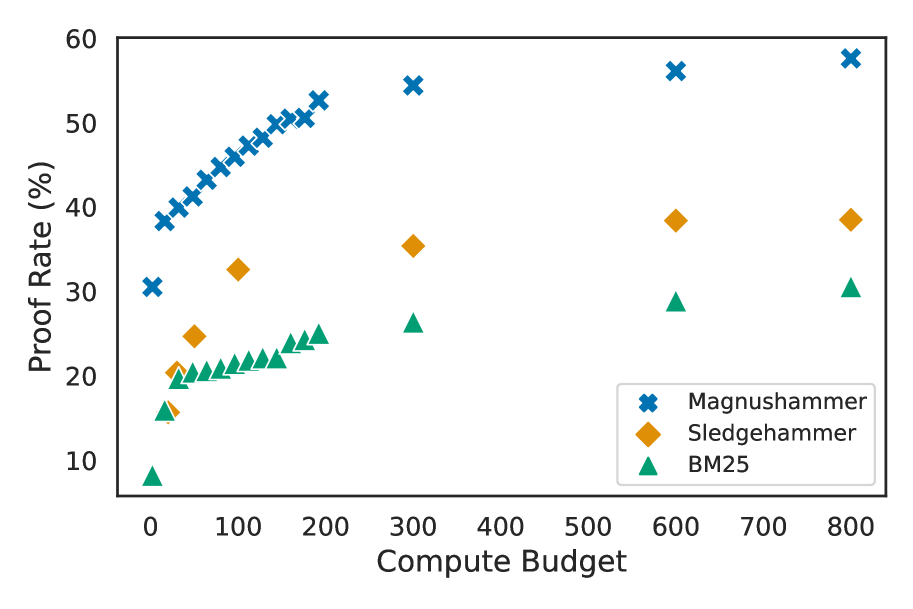
Figure 1: The proof success rate with varying computational budgets for Magnushammer, Sledgehammer, and BM25. Magnushammer shows remarkable scalability. Refer to Sections 5.1 for the definition of computational budget and Section 5.2.1 for configurations depicted in this figure.

Many tools have been developed to tackle premise selection (Alama et al., 2011; Kühlwein et al., 2012b; Kaliszyk et al., 2017; Bansal et al., 2019), including a broad class known as ”hammers”, which integrate Automated Theorem Provers (ATPs) into interactive proof assistants (Paulson & Blanchette, 2012; Gauthier & Kaliszyk, 2015; Kaliszyk & Urban, 2015a; Czajka & Kaliszyk, 2018). One such tool, known as Sledgehammer (SH) (Paulson & Blanchette, 2012), has gained prominence with Isabelle (Paulson, 2000), where it helped to create a significant portion of Isabelle’s proof corpus, the Archive of Formal Proofs. Although hammers have been integrated into other proof assistants (Gauthier & Kaliszyk, 2015; Czajka & Kaliszyk, 2018), they are not yet available in all proof assistants (Ebner, 2020): implementing hammers is a challenging task due to the varied structure of proof objects and the complex translation techniques required across different logics. Hence, there is a pressing need for an effective premise selection tool that can work seamlessly across all proof assistants with minimal adaptation requirements.

In this study, we provide a generic, data-driven transformer-based (Vaswani et al., 2017) premise selection tool, Magnushammer. We demonstrate that it can effectively handle premise selection while requiring little domain-specific knowledge. Magnushammer consists of two stages of retrieval, both trained using contrastive learning. Given a proof state, in the Select stage, we retrieve the most relevant $1024$ premises (measured by the cosine similarity of their embeddings) from hundreds of thousands of premises in the theorem (database up to 433K). In the second stage, Rerank, we re-rank the retrieved premises with more fine-grained but expensive processing: in a transformer architecture, we let the tokens from the proof state directly attend to the tokens of the retrieved premise, outputting a relevance score. An overview of Magnushammer is shown in Figure 3.

Magnushammer achieves a $59.5\%$ proof rate on the PISA benchmark (Jiang et al., 2021), a substantial improvement over Sledgehammer’s $38.3\%$ proof rate. We demonstrate that the proof rate of Magnushammer strongly dominates that of Sledgehammer given any compute budget, shown in Figure 1. Furthermore, we replace the Sledgehammer component in a neural-symbolic model Thor (Jiang et al., 2022a) with Magnushammer and improve the state-of-the-art proof rate from $57.0\%$ to $71.0\%$.

To achieve these results, we extracted a premise selection dataset from the Isabelle theorem prover and its human proof libraries. The dataset consists of $4.4$M examples of premise selection instances, with $433$K unique premises. To the best of our knowledge, this is the largest premise selection dataset of this kind.

Contributions

• We propose the use of transformers trained contrastively as a generic, data-driven approach for premise selection. Our method, Magnushammer, achieves a $59.5\%$ proof rate on the PISA benchmark, significantly improving the $38.3\%$ proof rate of Sledgehammer, the most popular symbolic premise selection tool.

• We extracted and released the largest, to the best of our knowledge, premise selection dataset. It consists of $4.4$M premise selection examples and $433$K unique premises. We hope this dataset can serve as an important tool for fostering future research in the area.

• We analyze how Magnushammer scales with the model size, dataset size, and the inference-time computational budget. Our evaluation indicates a promise for further improvements with more computing resources.

2 Background

2.1 Formal theorem proving

Interactive proof assistants such as Isabelle (Paulson, 2000) and Lean (de Moura et al., 2015) are software tools designed to assist the development of formal proofs. They provide expressive language for the formalization of mathematical statements and proofs while verifying them formally. In Isabelle, theorems are proved sequentially: an initial proof state is obtained after the theorem statement is defined, and the proof state changes when the user provides a valid proof step (see Appendix A.1 for an example theorem). Proof states contain information about the already established facts and the remaining goals to prove. Proof steps consist of tactics and (optionally) premises. Tactics are powerful theorem-proving decision procedures and can complete some proofs in one step provided with relevant premises (Alemi et al., 2016). However, finding these premises is difficult: one needs to select a handful of relevant facts from the current proof context. A typical proof context can contain tens of thousands of them.

2.2 Sledgehammer

Sledgehammer (Meng & Paulson, 2008; Paulson & Blanchette, 2012; Blanchette et al., 2013) is a powerful automated reasoning tool for Isabelle. Sledgehammer belongs to a broader class of tools known as “hammers”, which integrate Automated Theorem Provers (ATPs) into interactive proof assistants. The goal of these tools is to support the process of finding and applying proof methods. Sledgehammer has become an indispensable tool for Isabelle practitioners (Paulson & Blanchette, 2012). It allows for closing low-level gaps between subsequent high-level steps of proof without the need to memorize entire lemma libraries or perform a manual search.

Sledgehammer is designed to select relevant facts heuristically, translate them and the conjecture to first-order logic and try to solve the conjecture using ATPs. Examples of these ATPs are E (Schulz, 2004), SPASS (Weidenbach, 2001), Vampire (Riazanov & Voronkov, 2002), CVC5 (Barbosa et al., 2022), and Z3 (de Moura & Bjørner, 2008). If successful, these external provers generate complete proofs, but the proofs are not trusted by the Isabelle system. Instead, the facts used in the external proofs are extracted and used to reconstruct the proof using native Isabelle methods. This process is known as proof reconstruction (see Figure 2). This means that, in essence, Sledgehammer is a premise selection tool.

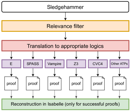
Figure 2: A call to Sledgehammer triggers the following sequence of steps: first, all available facts are filtered based on the symbolic similarity to the conjecture, then the conjecture, together with the selected facts (usually a few hundred of them), is translated to logics used by the external provers (E, SPASS etc.). Then they are fed into each ATP separately, and for each successful external proof, Isabelle tries to reconstruct it using its native methods.

2.2.1 Limitations of Sledgehammer

While immensely useful, Sledgehammer comes with several limitations. First, increasing computational power for Sledgehammer brings diminishing returns quickly (Böhme & Nipkow, 2010). Second, the necessary steps of logic projection and proof reconstruction for implementing a hammer are not straightforward for type systems other than higher-order logic (Czajka & Kaliszyk, 2018). Finally, Sledgehammer’s performance hinges on the relevance filtering scheme, a suite of methods based on handcrafted heuristics (Meng & Paulson, 2009) or classical machine learning (Kühlwein et al., 2013). Such approaches are unlikely to efficiently utilize the constantly growing body of proof data.

We argue that all these limitations can be overcome with deep-learning-based approaches. Neural networks have shown remarkable effectiveness in end-to-end problem solving with little or no feature engineering (Krizhevsky et al., 2012; Brown et al., 2020). Adopting textual representations with generic neural solutions removes the need for logic projection, ATP solving, and proof reconstruction. Moreover, Large Language Models have recently displayed impressive scaling properties with respect to both model size (Kaplan et al., 2020) and data (Hoffmann et al., 2022).

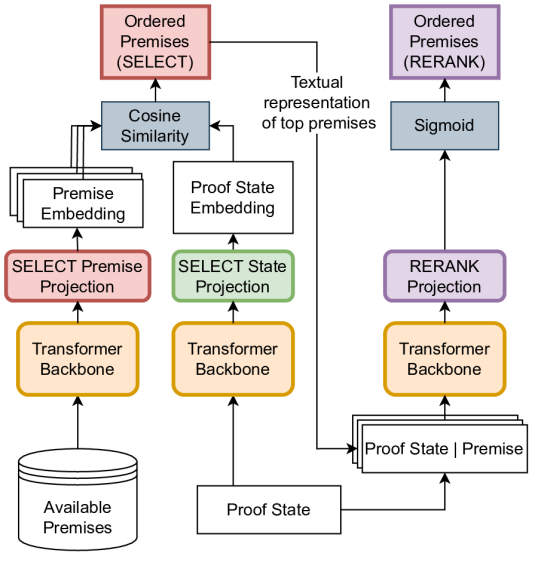
Figure 3: Overview of Magnushammer. Given a proof state, we first retrieve the most relevant premises according to the cosine similarity of their embeddings with the proof state embedding (Select). We then re-rank these with a model that encodes each proof state and premise pair, outputting a relevance score(Rerank). The bulk of the architecture is a shared transformer model, in orange.

3 Magnushammer

The goal of premise selection is to find relevant mathematical facts for a given proof state. We focus on selecting premises with a neural model informed by their textual representations instead of relying on proof object structures like Sledgehammer (Paulson & Blanchette, 2012) (see Section 2.2). The core idea of the Magnushammer method is to combine fast retrieval based on representational similarity (Select) with a more accurate re-ranking (Rerank), as outlined in Algorithm 1. Our method closely follows those of (Nogueira & Cho, 2019) and (Izacard et al., 2021). This hierarchical approach is scalable to large libraries, such as the tens of thousands of premises available in a typical proof context. Below we describe the two-stage Magnushammer method.

Select leverages representation similarity and is based on batch-contrastive learning similar to the methods of (Alemi et al., 2016; Bansal et al., 2019; Han et al., 2021; Radford et al., 2021). Select embeds premises and proof states into a common latent space and uses cosine similarity to determine their relevance. During inference, it requires only one pass of a neural network to compute the proof state embedding and dot product with cached premise embeddings. Select is hence fast and scalable to large sets of premises. In our experiments, there are between $30K$ and $50K$ premises in a typical proof state context, from which we select $K_{S}=1024$ most relevant ones.

Requires:

Algorithm 1 Magnushammer Premise Selection

$K_{S}$	# of premises to retrieve with Select
$K_{R}$	# of premises to retrieve with Rerank
$\mathtt{premises}$	database of premises

Input:
$\mathtt{proof\_state}$ to get premises for

  $\triangleright$ Select stage

  $\mathtt{state\_emb}\leftarrow\mathtt{get\_\textsc{Select}\_emb}(\mathtt{proof\_state})$

  $\mathtt{premise\_emb}\leftarrow\mathtt{get\_\textsc{Select}\_emb}(\mathtt{premises})$

  $\mathtt{Cache}(\mathtt{premise\_emb})$

  $\mathtt{sim\_scores}=\mathtt{state\_emb}\cdot\mathtt{premise\_emb}$

  $\mathtt{selected}=\mathtt{premises}[\mathtt{argsort(-sim\_scores)[:K_{S}]]}$

  $\triangleright$ Rerank stage

  $\mathtt{batch}=[]$

  for $\mathtt{premise}$ in $\mathtt{selected}$ do

     $\mathtt{batch}.append((\mathtt{proof\_state},\mathtt{premise}))$

  end for

  $\mathtt{scores}\leftarrow\mathtt{get\_}\textsc{Rerank}\mathtt{\_scores}(\mathtt{batch})$

  $\mathtt{top\_premises}=\mathtt{selected[argsort(-scores)[:K_{R}]]}$

  return $\mathtt{top\_premises}$

Rerank uses text similarity to score the relevance of premises to the current proof state by analyzing the full textual representation of $(\mathtt{proof\_state},\mathtt{premise})$ pairs. Rerank is trained to output the probability of the $\mathtt{premise}$ being relevant to the $\mathtt{proof\_state}$. The $K_{S}$ premises retrieved by Select are re-ranked with respect to these probabilities, and the final list comprises the top $K_{R}$ premises (we set $K_{R}=K_{S}$). Having both the premise and proof state in a single input allows Rerank to be more accurate, but, at the same time, it is much slower, as each pair must be scored individually.

Training

We train Magnushammer using two alternating tasks: Select trained with a modified InfoNCE loss (van den Oord et al., 2018), and Rerank with standard binary cross-entropy loss. The architecture of Magnushammer shares a transformer backbone with specialized linear projections on top (see Figure 3). The backbone is pre-trained with a language modeling task on the GitHub and arXiv subsets of The Pile dataset (Gao et al., 2021). For training, we use datasets consisting of $(\mathtt{proof\_state},\mathtt{premise})$ pairs extracted with a procedure described in Section 4.

During Select training, each batch consists of $N$ proof states, $N$ positive premises (one for each proof state), and additional $M$ negative premises sampled from available facts which are not ground truth premises for any of the selected proof states. This gives $N+M-1$ negatives per proof state. We typically use $M=3N$, which differs from standard batch-contrastive learning (Radford et al., 2021), in which $M=0$ and negatives are only the other $N-1$ premises in the batch (see Appendix B.3 for details). Rerank is trained using a binary classification objective. For each positive $(\mathtt{proof\_state},\mathtt{premise})$ pair in the dataset, we construct $15$ negatives from the most likely false positives returned by Select. Specifically, negative premises $\mathcal{M}$, which are facts that were never used as a premise for $\mathtt{proof\_state}$, are first chosen. Then, the top $1024$ of $\mathcal{M}$ according to Select are selected, and $15$ are sampled from them to construct negative pairs. The complete details of training and hyperparameter choices are in Appendix B.

Magnushammer evaluation in Isabelle

We outline how premises chosen by Magnushammer are used to prove theorems in Isabelle. Given a proof state, we retrieve the list of the $k$ most relevant premises $P$. We construct proof steps consisting of a tactic $t$ and a subset of premises $S\subset P$. Such proof steps are executed in parallel, with a timeout of $2$ seconds. The evaluation is successful if any of these proof steps completes the proof. For $S$, we pick the top $i$ of $P$, where $i$’s are consecutive powers of $2$ up to $2^{10}$ or $0$ for tactics that do not accept premises. The list of tactics used and the more detailed procedure description is presented in Appendix D. An example of a proof with tactics and premises is given in Appendix A.3.

Note that this procedure of trying different tactics and iterating over a subset of premises is very similar to the one implemented in Sledgehammer (Paulson & Blanchette, 2012). The rationale behind this is that the ATPs included in tactics perform combinatorial search, and providing them with fewer premises to restrict their search space is beneficial.

4 Datasets

We created and released a comprehensive dataset of textual representations for Isabelle’s proof states and premises. To the best of our knowledge, this is the first high-quality dataset of this kind for Isabelle. We used the two largest collections of Isabelle theories to create the dataset: the Archive of Formal Proofs and the Isabelle Standard library. See Appendix A.1 for a depiction of an example Isabelle proof.

For every proof step in the original proof, we collected the proof state and the premises used: a datapoint consists of a corresponding pair of $(\mathtt{proof\_state,premise})$. We call this the Human Proofs Library (HPL) dataset. In addition, we used Sledgehammer to generate proof steps that are different from human ones by using potentially alternative premises. We refer to this as the SH partition, and its union with HPL constitutes the Machine Augmented Proofs Library (MAPL) dataset. The number of datapoints, extracted proof states, and premises for both partitions are given in Table 1. MAPL grosses over $4$M datapoints.

Table 1: Statistics of both parts of the dataset: Human Proofs Library (coming from human-written proofs) and Sledgehammer (coming from generated proofs). Datapoints are $\mathtt{(proof\_state,premise)}$ pairs.

Dataset	HPL	SH	MAPL
Datapoints	1.1M	3.3M	4.4M
Unique proof states	570K	500K	570K
Unique premises	300K	306K	433K

We briefly describe how premises are extracted for each individual proof step. A proof in Isabelle is a sequence of tuples of the form $(\mathtt{proof\_state},\mathtt{proof\_step})$. The $\mathtt{proof\_state}$ has the state information, and $\mathtt{proof\_step}$ is a command that advances the proof. A $\mathtt{proof\_step}$ may use $\mathtt{premises}$: relevant theorems or lemmas established previously. Suppose a $\mathtt{proof\_step}$ contains $n$ premises $p_{1},p_{2},\ldots,p_{n}$, we then extract $n$ datapoints: $(\mathtt{proof\_state},p_{1})$, $(\mathtt{proof\_state},p_{2})$, $\cdots$, $(\mathtt{proof\_state},p_{n})$. Executing Sledgehammer on the $\mathtt{proof\_state}$ may result in multiple different synthetic $\mathtt{proof\_step}$s, and datapoints can be extracted from each in the same way (see Appendix A.2 for details). Mining the Human Proofs Library partition took $10$K CPU hours, and the SH partition took $150$K CPU hours (17 CPU years) on a distributed system.

Our datasets have $2$ distinguishing features:

1. Both $\mathtt{proof\_state}$s and $\mathtt{premise}$s are represented as text instead of richer structural representations, e.g., TPTP (Sutcliffe, 2017). This removes the need for feature engineering and allows cross-proof-assistant pre-training (Conneau & Lample, 2019).

2. We augment the human-written dataset by generating alternatives using Sledgehammer, which results in a significantly larger and more diverse dataset.

5 Experiments

We evaluate Magnushammer on the PISA and MiniF2F interactive theorem proving benchmarks using the proof success rate metric. Our main result is that Magnushammer outperforms Sledgehammer by a large margin and, combined with Thor (Jiang et al., 2022a), sets the new state of the art on the PISA benchmark ($71.0\%$ from $57.0\%$). Through ablations, we study the effectiveness of Magnushammer and the contribution of its training components. More experimental results and details can be found in Appendix E.

5.1 Experimental details

Benchmarks

In our experiments, we use two benchmarks: PISA (Jiang et al., 2021) and MiniF2F (Zheng et al., 2022). PISA contains problems randomly selected from the Archive of Formal Proofs; we use the same $1000$ problems as (Jiang et al., 2022a) for our evaluations. MiniF2F consists of $488$ high-school competition-level problems, split into a validation and test set, each with $244$ problems.

Metric and evaluation setups

In order to evaluate the performance, we measure proof success rate, which is the percentage of successful proofs. A proof generated by a given method is successful if it is formally verified by Isabelle. We distinguish single-step and multi-step settings. In the single-step setting, we check if the theorem can be proven in one step by applying premises retrieved by the evaluated premise selection method (e.g. Magnushammer). In the multi-step scenario, we perform proof search using a language model following Thor (Jiang et al., 2022a). Thor + Magnushammer uses Magnushammer instead of Sledgehammer as the premise selection component. A further explanation is given in Section 5.2.

In our experiments, we use the Portal-to-ISAbelle API (Jiang et al., 2021) to interact with Isabelle version 2021-1.

Evaluation protocol and computational budget

Algorithm 3 (Appendix D) details evaluation of Magnushammer in the single-step setting. It generates $|\mathcal{T}|\times|K|$ proof steps by combining a tactic $t\in\mathcal{T}$ with top $k\in K$ premises (provided by Magnushammer), where $\mathcal{T}$ is a prescribed set of tactics and $K$ is a list of integers. The proof is closed if any of the formulated proof steps are successful when executed in Isabelle. We define the computational budget for such evaluation as $C=|\mathcal{T}|\times|K|\times T$, where $T$ is a timeout expressed in seconds (we use $T=2$ as we observed little benefit from increasing it).

Estimating the computational budget for Sledgehammer is difficult due to its complex internal architecture. We approximate it by $C=S\times T$, where $S$ is the ‘number of CPU cores’ (corresponding to steps executed in parallel) and $T$ is the timeout. We use $S=10$ for our calculations. See also Appendix A.4 for more details.

Architecture and training details

For our main experiments, we pre-train standard decoder-only transformer models with $38$M and $86$M non-embedding parameters and fine-tune them for downstream tasks of premise selection or proof step generation. Full details are given in Appendix C.

5.2 Results on PISA and MiniF2F benchmarks

Our main empirical results, summarized in Table 2 and Table 3, were obtained with an $86$M non-embedding parameter model. Figure 1 and Section 5.2.1 deepen this study, showing that Magnushammer outperforms Sledgehammer across a broad spectrum of computational budgets.

Table 2: Proof rate on the PISA benchmark. On the single-step task, Magnushammer outperforms both Sledgehammer and BM25 by a wide margin. On the multi-step task, Magnushammer combined with Thor achieves the state-of-the-art proof rate of $71.0\%$.

	Method	Proof rate (%)
single	BM25	$30.6$
	Sledgehammer	$38.3$
	Magnushammer (Ours)	59.5
multi	LISA (Jiang et al., 2021)	$33.2$
	Thor (Jiang et al., 2022a)	$57.0$
	Thor + Magnushammer (Ours)	71.0

Table 3: Proof rate on the MiniF2F benchmark. On the single-step task, Magnushammer outperforms both Sledgehammer and its variant augmented with heuristics (Jiang et al., 2022b). On the multi-step task, Magnushammer combined with Thor obtains competitive results, in particular outperforming the original method. We emphasize that Magnushammer achieves comparable results using significantly smaller models. Thor + Magnushammer, Thor, and DSP use $2\times 86$M, $700$M, and $62$B parameters respectively.

	Method	valid (%)	test (%)
single	Sledgehammer	$9.9$	$10.4$
	Sledgehammer + heuristics	$18.0$	$20.9$
	Magnushammer (Ours)	33.6	34.0
multi	Thor (Jiang et al., 2022a)	$28.3$	$29.9$
	Thor + auto  (Wu et al., 2022a)	$37.3$	$35.2$
	Thor + Magnushammer (Ours)	$36.9$	$37.3$
	DSP (Jiang et al., 2022b)	43.9	39.3

Performance on the single-step task

In the single-step setting, Magnushammer outperforms Sledgehammer by a wide margin on both PISA ($59.5\%$ vs. $38.3\%$) and MiniF2F ($34.0\%$ vs. $20.9\%$). These findings indicate the potential for neural premise selection to replace traditional symbolic methods. Further, Magnushammer outperforms BM25 (when using the same evaluation protocol, see Algorithm 3), a text-based, non-trainable retrieval method (Robertson & Zaragoza, 2009) which is a strong baseline in common retrieval benchmarks (Thakur et al., 2021). This suggests that Magnushammer is able to learn more than just superficial text similarity. In these experiments, we use computational budget $1000$ as detailed in Appendix D.1.

Performance on the multi-step task

Neural theorem provers utilize language models to generate proof steps, following the approach proposed in (Polu & Sutskever, 2020). This allows for the creation of more complex, multi-step proofs. The proof generation involves sampling a proof step from the language model, verifying it, and repeating this process until the proof is closed or the computational budget is exceeded. A best-first search algorithm is often used to explore the most promising proof states.

Thor (Jiang et al., 2022a) augments neural theorem provers with premise-selection capabilities. To this end, Thor allows the model to generate proof steps using Sledgehammer, which we replace with Magnushammer (see Appendix D.2 for details). Thor+Magnushammer establishes a new state of the art on the PISA benchmark ($71.0\%$ vs. $57.0\%$). On MiniF2F, our method also significantly outperforms Thor and achieves results competitive with the current state of the art. In our experiments, we use a language model with $86$M non-embedding parameters. It is important to note that other theorem-proving approaches in the multi-step section of Table 3 require much larger language models (Thor: $700$M non-embedding parameters; DSP: $62$B parameters using Minerva (Lewkowycz et al., 2022)) and rely on ideas orthogonal to premise selection. Specifically, Thor + auto (Wu et al., 2022a) proposes a variation of Thor, involving expert iteration on auto-formalized data. Draft, Sketch and Prove (DSP) (Jiang et al., 2022b) involves creating a high-level outline of a proof and uses Sledgehammer to solve the low-level subproblems. We hypothesize that both methods would perform even better when combined with Magnushammer. In the multi-step experiments, we give Magnushammer a computational budget of $200$.

5.2.1 Scaling computational budget

In this section, we discuss how the quality of premise section methods varies with the computational budget available during evaluation. The results are in Figure 1 with a definition of the computational budget provided in Section 5.1. Notably, Magnushammer outperforms Sledgehammer even with very limited computational resources, and it scales well, particularly within the medium budget range.

For Magnushammer and BM25, we use Algorithm 3 (Appendix D) in various configurations (i.e., settings of $\mathcal{T}$ and $K$). We start with one tactic, $\mathcal{T}=\{\mathtt{smt}\}$, and $K=[2^{7}]$, which yields $C=2$ (recall that $T=2$). We then gradually add more tactics to $\mathcal{T}$ and more values to $K$. The final setup uses $|\mathcal{T}|=36$ and $K$ containing all powers of $2$, from $2^{0}$ up to $2^{10}$, which yields $C\approx 800$. Details are provided in Appendix D. For Sledgehammer, we scale the timeout parameter $T$ up to $80$.

5.3 Impact of training data

We study how the amount and type of data impact the proof rate by comparing Human Proofs Library (HPL) and Machine Augmented Proofs Library (MAPL) datasets. For this comparison, we used models with $38$M non-embedding parameters and a computational budget of $800$.

Dataset size

Our method is data-efficient; see Figure 4. We observe that Magnushammer fine-tuned on only $0.1\%$ of MAPL, equivalent to approximately $4$K samples, is already able to outperform Sledgehammer. This indicates that when starting from a pre-trained model, Magnushammer is a promising approach for addressing premise selection in theorem-proving environments with limited training data. The effect of pre-training diminishes as the amount of training data increases.

Dataset type

Fine-tuning on MAPL or HPL leads to subtle differences ($56.3\%$ vs. $54.0\%$ when the whole datasets are used). This outcome may be attributed to the impact of model pre-training and the fact that the HPL dataset is rich enough to obtain good performance on the PISA benchmark (as observed in the previous paragraph). We speculate that the bigger MAPL dataset might be essential for future harder benchmarks and scaling up the model size.

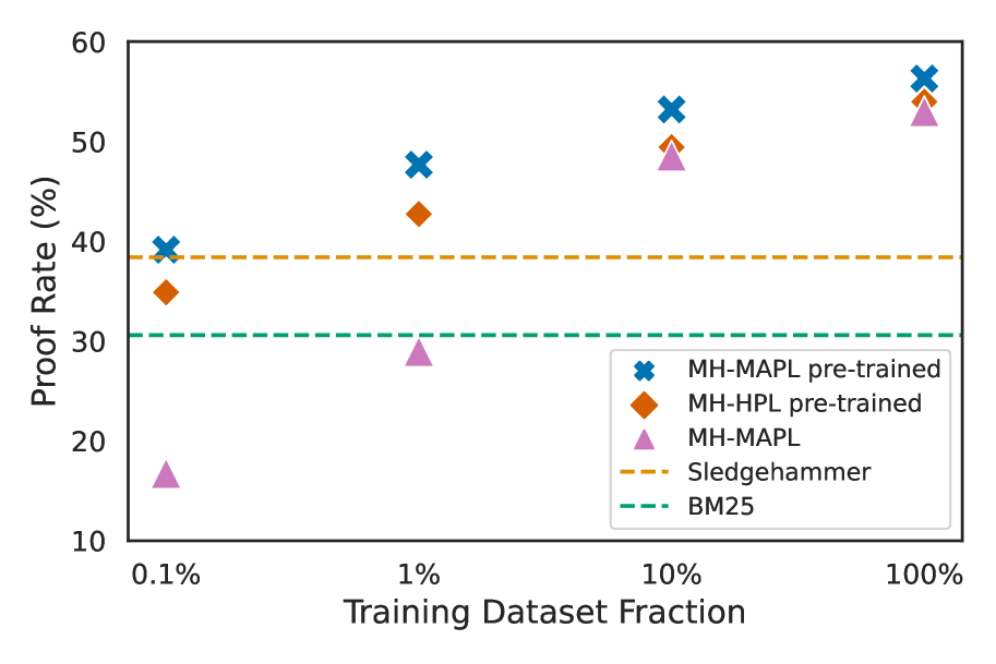
Figure 4: Impact of the training data on the proof rate. We randomly sample a fraction of MAPL or HPL datasets and use it for training the model. Just $0.1\%$ of the MAPL dataset allows Magnushammer to outperform the Sledgehammer. See Table 4 (Appendix E.1) for numerical data.

5.4 Ablations

In ablations, we use models trained on the MAPL dataset and evaluate them with the computational budget of $800$.

Model Size

To study how the performance of our method depends on the model size, we vary the number of layers $L$ and embedding dimension $D$ (see Appendix C.1 for architectural details). A positive correlation between the model size and the proof rate is shown in Figure 5. We observe that even a tiny model with $920$K parameters ($L=1,D=256$) outperforms Sledgehammer ($40.7\%$ vs. $38.3\%$). We also note the benefit of pre-training and that scaling the number of layers is more beneficial than scaling the embedding dimension. Details, including the configuration of each model, are in Appendix C.1.

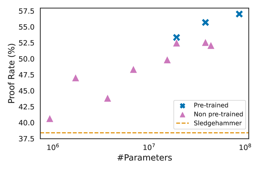
Figure 5: Dependence of the proof rate on the model size. Even with a tiny one-layer transformer Magnushammer outperforms the Sledgehammer, achieving $40.7\%$ proof rate compared to $38.3\%$. We observe consistent gains when increasing the model size and further benefit from using the pre-trained models. For numerical data refer to Table 5 (Appendix E.1).

Impact of Re-Ranking

We find that the Select-only method, i.e., Magnushammer without the Rerank phase, already significantly outperforms Sledgehammer. Tested on the $38$M model, it achieves a $54.2\%$ proof rate comparable to $56.3\%$ obtained by Magnushammer. Select-only is a computationally appealing alternative, as it only needs a single forward pass to embed the current proof state. Premise embeddings can be pre-computed and cached, allowing inference on the CPU without the need for GPU or TPU accelerators.

6 Related work

Existing works on premise selection use models based on classical ML like Bayesian methods (Kühlwein et al., 2012a), decision trees (Nagashima & He, 2018), and more recently, deep learning. Effective deep learning approaches typically leverage the structure of mathematical expressions using graph neural networks (Wang et al., 2017; Paliwal et al., 2020; Goertzel et al., 2022). Our work uses the transformer architecture (Vaswani et al., 2017), which is highly scalable and capable of producing powerful representations of text data. Unlike traditional hammers (Paulson & Blanchette, 2012; Kaliszyk & Urban, 2015a; Gauthier & Kaliszyk, 2015; Czajka & Kaliszyk, 2018; Goertzel et al., 2022), our method does not depend on external automated theorem provers and requires little domain-specific knowledge.

Pre-trained transformer language models have been applied to various aspects of theorem proving, including tactic prediction (Yang & Deng, 2019), proof step search (Polu & Sutskever, 2020; Lample et al., 2022), and autoformalization (Wu et al., 2022a; Jiang et al., 2022b). The application of generative language models to premise selection has been limited, as the length of the possible premises often greatly exceeds the context of several thousand tokens that the models are designed to handle. Jiang et al. (2022a) circumvents the difficulty of premise selection by invoking Sledgehammer. In contrast, Magnushammer retrieves rather than generates to overcome the context length limitation. Therefore it can be used in tandem with other models (we demonstrate its combination with Thor (Jiang et al., 2022a) in Section 5).

Batch-contrastive learning is widely used in speech (van den Oord et al., 2018), text (Izacard et al., 2021), image (Chen et al., 2020) and image-text representation learning (Radford et al., 2021). The Select phase of our premise selection model relies on in-batch negative examples to train the retrieval, similarly to Holist (Bansal et al., 2019) and Contriever (Izacard et al., 2021). Just like Holist, we sample additional negatives for each proof state, which we have found crucial for good performance. The Rerank stage closely resembles (Nogueira & Cho, 2019), but instead of using BM25 as the initial retrieval phase, we jointly train retrieval and re-ranking, utilizing premises retrieved by Select as hard negatives for Rerank training.

There are multiple lines of work considering datasets based on formal theorem proving, such as theorem proving benchmarks for Isabelle, Lean, and other environments (Zheng et al., 2022; Azerbayev et al., 2022). These datasets only focus on evaluation, not providing data for training the models. Another line of research focuses on benchmarking machine learning models’ reasoning capabilities while also providing training data (Bansal et al., 2019; Li et al., 2021; Han et al., 2022). Existing public datasets for premise selection include the ones introduced in (Piotrowski & Urban, 2020; Goertzel et al., 2022). In comparison to these works, we publish the data in textual format, as seen in Isabelle, instead of translated, structured formats such as Thousands of Problems for Theorem Provers (Sutcliffe, 2017). On top of that, we contribute additional proofs generated with Sledgehammer, which increase both the size and the diversity of the data.

7 Limitations and further work

Other proof assistants Magnushammer treats proof states and premises as text and makes no assumptions about their structure. As such, it can be applied to any theorem-proving environment, provided that a large enough dataset is available. We conjecture that, due to their textual format, our HPL and MAPL datasets can be used for pre-training models for proof assistants other than Isabelle, which we leave for future work.

Better proof and premise representations Magnushammer utilizes the textual representation of the proof state given by Isabelle. This representation, however, does not provide complete information about the referenced objects; including function definitions or object types in the proof state might further improve performance.

Language models for premise selection Combining language models with external premise selection tools significantly improves their theorem-proving performance, as demonstrated by (Jiang et al., 2022a) and our work. A natural step would be to further integrate premise selection with language models into a single model capable of generating proof steps containing relevant retrieved premises. A proof of concept of this idea was explored in (Tworkowski et al., 2022). We believe that recent advances in retrieval-augmented language models (Wu et al., 2022b; Borgeaud et al., 2022) could facilitate progress in this direction.

8 Conclusion

In this paper, we introduced Magnushammer, a neural premise selection method that is transferable across proof assistants. We evaluate it in the Isabelle environment, showing that it outperforms the popular tool Sledgehammer on two benchmarks: PISA and MiniF2F. Magnushammer can be plugged into automated reasoning systems as the premise selection component, as showcased with Thor. With its ease of adoption and high performance even with a low computational budget, Magnushammer paves the way for the firmer integration of deep-learning-powered tools into proof assistants.

Appendix

Appendix A Isabelle environment

This section contains visual examples of proofs in Isabelle and provides some configuration details of the environment.

A.1 Visualization of the Isabelle environment

The following is an example theorem, as presented in Isabelle’s most popular IDE, jEdit. The theorem comes from an AFP entry Fun With Functions (Nipkow, 2008) and states that any mapping $f$ from the set of natural numbers to itself that satisfies $f(f(n))<f(n+1)$ must be the identity function. The proof starts with a simple induction and then refines the result to arrive at the thesis. This problem was included in Terence Tao’s 2006 booklet Solving Mathematical Problems (Tao, 2010).

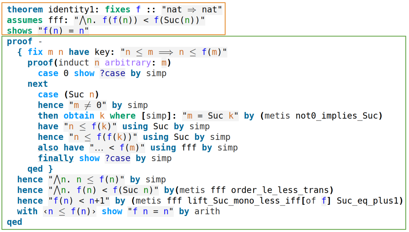
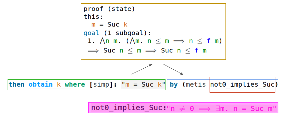
Figure A.1: An example theorem in Isabelle. The statement is highlighted in the orange frame and the body of the proof is in the green frame. In this proof, most of the lines contain two consecutive steps: the first formulates a new proposition, and the second proves it. See the analysis of steps from line 20 below.

Figure A.2: The line is broken down into two steps: the first one (green frame) includes the proposition (since $m$ is natural and positive, it must have a predecessor $k$) and the second (blue frame) proves it using the tactic metis with premise not0_implies_Suc, that states that a nonnegative natural number is a successor of some other natural number. The used premise is a fact which is already defined in the lemma library. The proof state resulting from the first step is in the yellow frame. The full premise statement is highlighted in pink.

A.2 Alternative proof step generation with Sledgehammer

This section describes how to generate alternative proof steps using Sledgehammer which we do to obtain datasets described in Section 4. First, we find all intermediate propositions within the proof (they can be nested) and try to replace the proof of the proposition with a Sledgehammer step. If successful, we record such a step in the dataset and proceed with both the original and the alternative proof. Figure A.3 provides a visual example of the aforementioned propositions.

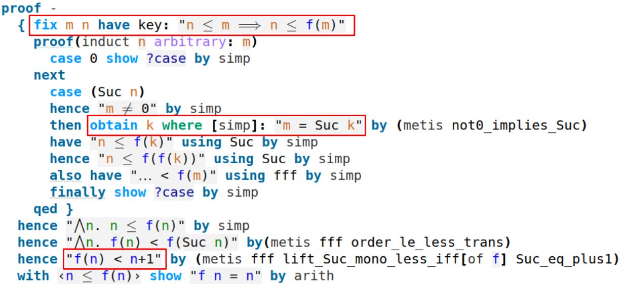
Figure A.3: Example intermediate propositions highlighted in red. Note: not all propositions were highlighted.

A.3 Example of a proof with tactics requiring premises

Figure A.4 contains a multi-step proof of the irrationality of $\sqrt{2}$ written in Isabelle. The proof contains multiple usages of tactics that require premises.

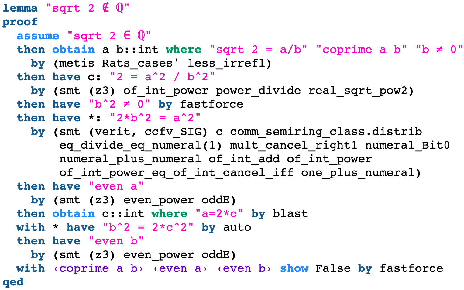
Figure A.4: A proof of $\sqrt{2}\notin\mathbb{Q}$ (Jiang et al., 2022a, Figure 1). The steps containing metis, smt, fastforce, blast, auto, fastforce are examples of steps using premises. For instance, one such proof step is by (metis Rats_cases’ less_irrefl). This step invokes metis and provides two premises as arguments, namely Rats_cases’ and less_irrefl.

A.4 Sledgehammer setup

We set up Sledgehammer in Isabelle 2021-1, following the configuration from (Jiang et al., 2022a). We run Sledgehammer using different sets of settings and calculate the total proof rate by taking the union of problems solved by each run. The Sledgehammer timeout is set to default $30$ seconds. We use only on-machine automated theorem provers (same as Isabelle environment), so external provers used by Sledgehammer are the following: Z3, SPASS, Vampire, CVC4, and E.

In our calculation of the Sledgehammer computation budget, see Section 5.1, we assume $S=10$ ’CPU cores’. We run our experiments on machines with $96$ CPU cores, making the assumption realistic. Moreover, we emphasize that the performance gap between Magnushammer and Sledgehammer is large enough that altering the value of $S$, e.g., to an unrealistic level $S=1$, would not qualitatively change conclusions.

Appendix B Details of Magnushammer

B.1 Select

Select stage is trained using the InfoNCE loss (van den Oord et al., 2018) defined as:

$$\mathcal{L}\left(q,k_{+}\right)=-\frac{\exp\left(s\left(q,k_{+}\right)/\tau\right)}{\exp\left(s\left(q,k_{+}\right)/\tau\right)+\sum_{i=1}^{K}\exp\left(s\left(q,k_{i}\right)/\tau\right)},$$

where $q$ is a query (a proof state), $k_{+}$ is a positive premise (a ground truth from the dataset), $k_{i}$ are negative premises. We define $s$ as cosine similarity between proof state and premise embeddings; $\tau>0$ is a non-trainable temperature parameter. We list our hyperparameter choices in section C.2.

B.2 Rerank

Premise retrieval task can be cast as binary classification, trying to determine if a given pair $(\mathtt{proof\_state},\mathtt{premise})$ is relevant. Applying classification to each pair is computationally infeasible, however, it could be used to re-rank a small set of premises retrieved by Select. Namely, we use the following cross-entropy loss:

$$\mathcal{L}=-\sum_{p\in\mathcal{P}}\log\mathtt{score}(p)-\sum_{p\notin\mathcal{N}}\log(1-\mathtt{score}(p)),$$

where $\mathtt{score}(p)$ is the output of the Rerank part of the model (see ”Sigmoid” in Figure 3) for a given $p=(\mathtt{proof\_state},\mathtt{premise})$ pair. Typically, we sample a batch of $16$ positive pairs $\mathcal{P}$ from the dataset. For each such pair $(\mathtt{proof\_state},\mathtt{premise})$ $15$ negatives are constructed from the most likely false positives returned by Select. Specifically, negative premises $\mathcal{\mathcal{M}}$, which are facts that were never used as a premise for $\mathtt{proof\_state}$, are first chosen. Then, the top $1024$ of $\mathcal{M}$ according to Select are selected, and $15$ are sampled from them to construct negative pairs, which are included in $\mathcal{N}$.

B.3 Magnushammer

We train Magnushammer as two separate tasks alternating update steps as presented in Algorithm 2. Note that the backbone of the architecture is shared between Select and Rerank, thus such multi-task training is potentially more effective than having two separate models. Calculation of the negative premises for Select is costly, thus for efficiency reasons we recalculate the top $1024$ premises, see Section B.2, every $T=1000$ steps in the $\mathtt{recompute\_negatives\_for\_rerank}$ function, as outlined in the Algorithm 2.

Algorithm 2 Magnushammer Training

Requires:	$\theta$	initial parameters
	$D$	premise dataset
	$T$	interval for updating rerank dataset

  $D\mathtt{{}_{rerank}}\leftarrow$ $\mathtt{recompute\_negatives\_for\_rerank}$$(\theta,D)$

  $\mathtt{step}=0$

  while $\mathtt{step}<\mathtt{num\_train\_steps}$ do

     $\mathtt{batch\_select}\leftarrow D\mathtt{.sample()}$

     $\mathtt{\theta}\leftarrow$ train_step$\mathtt{(\theta,batch\_select)}$

     $\mathtt{batch\_rerank}\leftarrow D\mathtt{{}_{rerank}.sample()}$

     $\mathtt{\theta}\leftarrow$ train_step$\mathtt{(\theta,batch\_rerank)}$

     $\mathtt{step}\leftarrow\mathtt{step}+1$

     if $\mathtt{step}\mod T=0$ then

        $D\mathtt{{}_{rerank}}\leftarrow$ $\mathtt{recompute\_negatives\_for\_rerank}$$(\theta,D)$

     end if

  end while

Appendix C Training details

C.1 Model architecture

We use a decoder-only transformer architecture, following the setup from (Wang & Komatsuzaki, 2021) and using rotary position embedding (Su et al., 2021), a variation of relative positional encoding. The feedforward dimension in the transformer block is set to $4\times D$ where $D$ denotes embedding dimension, and the number of attention heads is $H=D/64$. Our $38$M model has $L=12$ layers and an embedding dimension of $D=512$. The larger $86$M model consists of $L=12$ layers and has $D=768$. For all the models, we use the original GPT-2 tokenizer (Radford et al., 2019).

In Select, we append a specialized token at the end of the sequence to compute the embedding for a proof state and linearly project its embedding. Premises are embedded analogously. Similarly to (Radford et al., 2021) that trains separate projections for images and captions, we train separate proof state and premise projections and share the transformer backbone (see Figure 3). Analogously for Rerank, we compute the relevance score by taking the embedding of the last token and then projecting it to a scalar value.

C.2 Hyperparameter setup

We performed the following hyperparameter sweeps. We note that we have not observed significant differences between obtained results.

• Learning rate: $\{{1}\mathrm{e}{-4},{2}\mathrm{e}{-4},{3}\mathrm{e}{-4},{5}\mathrm{e}{-4}\}$, chosen: ${2}\mathrm{e}{-4}$

• Dropout: $\{0.0,0.05,0.1,0.2\}$, chosen: $0.1$

• Weight decay: $\{0.02,0.05,0.1\}$, chosen: $0.02$

• Batch size $N$ in Select: $\{128,256,512\}$, chosen: $256$

• Number of negatives $M$ in Select: $\{0,256,768,1536\}$, chosen: $768$

• Temperature for InfoNCE loss in Select: $\{0.05,0.07,0.2,1\}$, chosen: $0.07$

• Batch size for Rerank: $\{16,32,64\}$, chosen $64$

• Number of negatives per proof state $\mathcal{M}$ in Rerank: $\{7,15\}$, chosen: $15$.

C.3 Pre-training on language modeling

Pre-training has been shown to dramatically increase the capabilities and performance of decoder-only models on tasks other than language modeling (Howard & Ruder, 2018). Motivated by that, we pre-train our models on GitHub, and arXiv subsets of The Pile (Gao et al., 2021). The models are trained for $1$M steps, with a context length of $2048$. Global batch size is set to $32$ sequences giving a total number of $65536$ tokens per batch. Dropout is disabled, and weight decay is set to $0.02$. The learning rate increases linearly from $0$ to $0.0003$ for the first $10000$ steps, and then the cosine schedule is applied to decrease its value gradually.

C.4 Fine-tuning for downstream tasks

We train Magnushammer by taking a pre-trained language model, removing its language modeling head, and attaching three linear projections heads - one projection for proof state embedding, another one for premise embedding, and the last one for producing relevance score for Rerank, as depicted in Figure 3 and described in Section C.1. For the proof step generation task, we fine-tune our language models by applying the algorithm used to train Thor (Jiang et al., 2022a).

C.5 Hardware

We gratefully acknowledge that our research was supported with Cloud TPUs from Google’s TPU Research Cloud (TRC). We use TPU virtual machines from the Google Cloud Platform (GCP) for all stages: pre-training, fine-tuning, and evaluation. Each TPU virtual machine has 8 TPU v3 cores, 96 CPU cores, and over 300GB of RAM. TPU v3 cores have around 16GB of memory each. The Isabelle environment is set to have access to 32 CPU cores.

Appendix D Magnushammer evaluation

Below, in Algorithm 3 we outline our evaluation method described in Section 5.1. To generate proof steps, we use the following tactics: smt, metis, auto, simp, blast, meson, force, eval, presburger, linarith. Algorithm 3 is also used to evaluate BM25, where we select $\mathtt{top\_premises}$ with this retrieval method instead of Magnushammer.

D.1 Computational budget

For our main result (Section 5.2), we allocate the computational budget of $1000$ as follows: apart from the powers of two from $2^{0}$ to $2^{10}$, we also try the following $k$ values: $\left[48,96,192\right]$, which in total gives $14$ values. With each of these $k$ values, $36$ tactics are used with timeout $T=2$, yielding $C\approx 1000$.

For the ablation studies, we only use powers of two from $2^{0}$ to $2^{10}$, and the same set of $36$ tactics, which gives $C\approx 800$.

Requires:

Algorithm 3 Magnushammer Evaluation in ITP

Magnushammer	premise selection model
$K_{S}$	# of premises to retrieve with Select
$K_{R}$	# of premises to retrieve with Rerank
$\mathtt{premises}$	available premises
$\mathtt{top\_k\_premises\_to\_try}$	list with the number of top premises to generate steps with
$\mathtt{tactics\_to\_try}$	list of tactics to generate steps with
$\mathtt{env}$	interactive theorem proving environment (e.g. Isabelle)

Input:
$\mathtt{theorem}$ to prove

  $\triangleright$ INITIALIZE PROBLEM AND GET TOP PREMISES

  $\mathtt{proof\_state}\leftarrow$ init_problem$(\mathtt{env},\mathtt{theorem})$

  $\mathtt{top\_premises}\leftarrow$ Magnushammer $({\mathtt{proof\_state}},\mathtt{premises},K_{S},K_{R})$

  $\triangleright$ GENERATE PROOF STEPS CONSISTING OF TACTICS AND TOP K PREMISES

  $\mathtt{steps}$ = []

  for $\mathtt{k}$ in $\mathtt{top\_k\_premises\_to\_try}$ do

     $\triangleright$ SELECT BEST K PREMISES

     $\mathtt{top\_k\_premises}\leftarrow$ $\mathtt{top\_premises[:k]}$

     $\triangleright$ GENERATE ATPs STEPS WITH PREMISES

     $\mathtt{new\_steps}\leftarrow$generate_steps$(\mathtt{tactics\_to\_try},\mathtt{top\_k\_premises})$

     $\mathtt{steps}.append(\mathtt{new\_steps})$

  end for

  $\triangleright$ APPLY GENERATED PROOF STEPS IN THE ENVIRONMENT

  $\mathtt{solved}\leftarrow$ try_steps$({\mathtt{env,steps}})$

  return $\mathtt{solved}$

D.2 Thor + Margnushammer

To generate more complex proofs we combine Thor (Jiang et al., 2022a) with Magnushammer as introduced in multi-step setting in Section 5.2.

Firstly, we follow the procedure described in (Jiang et al., 2022a) to pre-process training data and fine-tune our pre-trained language model for the proof generation task (pre-training details can be found in Appendix C.3). To evaluate the combination Thor+Magnushammer we assume parallel execution of steps generated by Magnushammer. Namely, we assign a constant cost of $15$ seconds per application of steps generated by Magnushammer to emulate parallel verification of these steps.

We then assign the same computational budget as proposed in Thor, with the only difference being that each proof step has a timeout limit of $2$s (instead of $10$s), which we found to perform better in our setup. The search is terminated if and only if one of the following scenarios happens: (1) a valid proof has been found for the theorem; (2) the language model is queried 300 times; (3) a wall-time timeout of $500$s has been reached (assuming parallel execution of Magnushammer steps); (4) the queue is empty but the theorem is not proved. We keep the same maximum length of the queue equal to $32$.

Appendix E Additional experimental results

E.1 Supplemental details

We provide additional details for our main experiments and ablations.

Table 4: Relation between the training data and the proof rate discussed in Section 5.3 and Figure 4.

Dataset	Fraction	Pre-trained	Proof rate (%)
MAPL	$0.1\%$	Yes	$39.2$
HPL	$0.1\%$	Yes	$34.9$
MAPL	$0.1\%$	No	$16.8$
MAPL	$1\%$	Yes	$47.7$
HPL	$1\%$	Yes	$42.7$
MAPL	$1\%$	No	$29.0$
MAPL	$10\%$	Yes	$53.2$
HPL	$10\%$	Yes	$49.4$
MAPL	$10\%$	No	$48.5$
MAPL	$100\%$	Yes	$56.3$
HPL	$100\%$	Yes	$54.0$
MAPL	$100\%$	No	$53.0$

Table 5: Proof rate on PISA for different models discussed in Section 5.4 and Figure 5. We vary the number of layers $L$ and the embedding dimension $D$ of the Transformer model.

Transformer $(L,D)$	#Parameters	Pre-trained	Proof rate (%)
$(1,256)$	$920$K	No	$40.7$
$(1,512)$	$3.7$M	No	$43.9$
$(2,256)$	$1.7$M	No	$47.0$
$(2,512)$	$6.8$M	No	$48.4$
$(2,768)$	$15.4$M	No	$49.9$
$(6,512)$	$19.2$M	No	$52.5$
$(6,512)$	$19.2$M	Yes	$53.3$
$(6,768)$	$43.7$M	No	$52.1$
$(12,512)$	$38.3$M	No	$52.6$
$(12,512)$	$38.3$M	Yes	$56.3$
$(12,768)$	$86.2$M	Yes	$57.0$

E.2 Step tactic prompt

We observed that different tactics use different subsets of premises. This motivated us to extend the context given to our model with tactic prompt. Namely, provide the tactic name as an additional argument to the premise selection model, similarly to (Bansal et al., 2019). Prompting model with the tactic name does not yield significant improvements. However, it allows the model for a more accurate premise selection. Namely, as presented in Figure A.5 and Table 6, we observe that premises necessary to close the proof are ranked higher. This motivates an alternative performance metric presented in the next section.

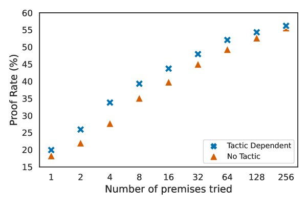
Figure A.5: We calculate accumulated proof rate in the following way: try 1 premise, count problems solved, then try 2 premises, count problems solved using 1 or 2 premises, then try 4 premises, count problems solved using 1, 2, or 4 premises etc. Following this, on the x-axis we have the number of premises used to generate steps in Algorithm 3. The y-axis presents the accumulative proof rate as we try more and more premises. The higher the proof rate for the smaller number of premises used the better. We observe that prompting the model with the tactic is not necessary to achieve the final high proof. However, it allows the model for a more accurate premise selection - all premises necessary to close the proof are ranked higher.

Table 6: Effect of the number of premises used for generating tactic steps on the proof rate. We fix a set of tactics and accumulate problems solved as we increase the number of premises used to generate steps in Algorithm 3. Namely, for each $k$, we count the number of problems solved using at most $k$ premises. The “Tactic” column indicates whether the model was given a tactic prompt.

Model	Tactic	Dataset	$k\leq 0$	$\leq 1$	$\leq 2$	$\leq 4$	$\leq 8$	$\leq 16$	$\leq 32$	$\leq 64$	$\leq 128$	$\leq 256$
BM25	No	N/A	9.63	13.56	15.62	16.7	18.47	20.73	23.38	25.44	28.0	30.55
MH-86M	No	HPL	9.63	19.25	22.99	28.68	34.58	39.88	44.5	47.84	51.47	52.95
MH-86M	Yes	HPL	9.63	20.24	25.44	31.53	36.15	40.67	44.7	48.53	51.87	54.22
MH-86M	No	MAPL	9.63	18.27	22.0	27.7	35.07	39.78	44.99	49.31	52.65	55.6
MH-86M	Yes	MAPL	9.63	19.94	25.93	33.79	39.29	43.71	47.94	52.06	54.32	56.19

E.3 Number of premises used as a performance metric for premise selection.

Consider the number of premises used to generate steps in Algorithm 3 (parameter $k$ in the for-loop). Intuitively, the fewer premises needed the better, since it means that all the premises necessary to close the proof are ranked higher (high recall), thus the model does a more accurate premise selection. In other words, a better retrieval model should be able to score all the necessary facts higher and push unnecessary facts down the list.

To compare different models we fix a set of tactics and accumulate problems solved as we increase the number of premises used to generate steps in Algorithm 3. This is presented in Table 6 and Figure A.5. Namely, for each $k$, we count the number of problems solved using at most $k$ premises. Effectively, each new value of $k$ adds one new step per tactic to try.

E.4 Single-step proof rate bound

It is non-trivial to estimate the lower bound on how many problems can be closed directly from the root state in a single proof step. To answer this question, we use different models in Algorithm 3 and take the union of problems solved by them. Namely, we ensemble the results of the Magnushammer variations introduced in previous sections: Magnushammer-86M, Magnushammer-38M, Magnushammer-Select, Sledgehammer, BM25, and the models presented in Section 5.4. Such a combination successfully closes $65.5\%$ of the proofs.

References

- Alama et al. (2011) Alama, J., Kühlwein, D., Tsivtsivadze, E., Urban, J., and Heskes, T. Premise selection for mathematics by corpus analysis and kernel methods. CoRR, abs/1108.3446, 2011. URL http://arxiv.org/abs/1108.3446.
- Alemi et al. (2016) Alemi, A. A., Chollet, F., Irving, G., Szegedy, C., and Urban, J. Deepmath - deep sequence models for premise selection. CoRR, abs/1606.04442, 2016. URL http://arxiv.org/abs/1606.04442.
- Azerbayev et al. (2022) Azerbayev, Z., Piotrowski, B., and Avigad, J. Proofnet: A benchmark for autoformalizing and formally proving undergraduate-level mathematics problems. In Advances in Neural Information Processing Systems 35, 2nd MATH-AI Workshop at NeurIPS’22, 2022. URL https://mathai2022.github.io/papers/20.pdf.
- Bansal et al. (2019) Bansal, K., Loos, S. M., Rabe, M. N., Szegedy, C., and Wilcox, S. Holist: An environment for machine learning of higher order logic theorem proving. In Chaudhuri, K. and Salakhutdinov, R. (eds.), Proceedings of the 36th International Conference on Machine Learning, ICML 2019, 9-15 June 2019, Long Beach, California, USA, volume 97 of Proceedings of Machine Learning Research, pp. 454–463. PMLR, 2019. URL http://proceedings.mlr.press/v97/bansal19a.html.
- Barbosa et al. (2022) Barbosa, H., Barrett, C. W., Brain, M., Kremer, G., Lachnitt, H., Mann, M., Mohamed, A., Mohamed, M., Niemetz, A., Nötzli, A., Ozdemir, A., Preiner, M., Reynolds, A., Sheng, Y., Tinelli, C., and Zohar, Y. cvc5: A versatile and industrial-strength SMT solver. In Fisman, D. and Rosu, G. (eds.), Tools and Algorithms for the Construction and Analysis of Systems - 28th International Conference, TACAS 2022, Held as Part of the European Joint Conferences on Theory and Practice of Software, ETAPS 2022, Munich, Germany, April 2-7, 2022, Proceedings, Part I, volume 13243 of Lecture Notes in Computer Science, pp. 415–442. Springer, 2022. doi: 10.1007/978-3-030-99524-9“˙24. URL https://doi.org/10.1007/978-3-030-99524-9_24.
- Blanchette et al. (2013) Blanchette, J. C., Böhme, S., and Paulson, L. C. Extending sledgehammer with SMT solvers. J. Autom. Reason., 51(1):109–128, 2013. doi: 10.1007/s10817-013-9278-5. URL https://doi.org/10.1007/s10817-013-9278-5.
- Böhme & Nipkow (2010) Böhme, S. and Nipkow, T. Sledgehammer: Judgement day. In Giesl, J. and Hähnle, R. (eds.), Automated Reasoning, pp. 107–121, Berlin, Heidelberg, 2010. Springer Berlin Heidelberg. ISBN 978-3-642-14203-1.
- Borgeaud et al. (2022) Borgeaud, S., Mensch, A., Hoffmann, J., Cai, T., Rutherford, E., Millican, K., van den Driessche, G., Lespiau, J., Damoc, B., Clark, A., de Las Casas, D., Guy, A., Menick, J., Ring, R., Hennigan, T., Huang, S., Maggiore, L., Jones, C., Cassirer, A., Brock, A., Paganini, M., Irving, G., Vinyals, O., Osindero, S., Simonyan, K., Rae, J. W., Elsen, E., and Sifre, L. Improving language models by retrieving from trillions of tokens. In Chaudhuri, K., Jegelka, S., Song, L., Szepesvári, C., Niu, G., and Sabato, S. (eds.), International Conference on Machine Learning, ICML 2022, 17-23 July 2022, Baltimore, Maryland, USA, volume 162 of Proceedings of Machine Learning Research, pp. 2206–2240. PMLR, 2022. URL https://proceedings.mlr.press/v162/borgeaud22a.html.
- Brown et al. (2020) Brown, T. B., Mann, B., Ryder, N., Subbiah, M., Kaplan, J., Dhariwal, P., Neelakantan, A., Shyam, P., Sastry, G., Askell, A., Agarwal, S., Herbert-Voss, A., Krueger, G., Henighan, T., Child, R., Ramesh, A., Ziegler, D. M., Wu, J., Winter, C., Hesse, C., Chen, M., Sigler, E., Litwin, M., Gray, S., Chess, B., Clark, J., Berner, C., McCandlish, S., Radford, A., Sutskever, I., and Amodei, D. Language models are few-shot learners, 2020. URL https://arxiv.org/abs/2005.14165.
- Chen et al. (2020) Chen, T., Kornblith, S., Norouzi, M., and Hinton, G. E. A simple framework for contrastive learning of visual representations. In Proceedings of the 37th International Conference on Machine Learning, ICML 2020, 13-18 July 2020, Virtual Event, volume 119 of Proceedings of Machine Learning Research, pp. 1597–1607. PMLR, 2020. URL http://proceedings.mlr.press/v119/chen20j.html.
- Conneau & Lample (2019) Conneau, A. and Lample, G. Cross-lingual language model pretraining. In Wallach, H., Larochelle, H., Beygelzimer, A., d'Alché-Buc, F., Fox, E., and Garnett, R. (eds.), Advances in Neural Information Processing Systems, volume 32. Curran Associates, Inc., 2019. URL https://proceedings.neurips.cc/paper/2019/file/c04c19c2c2474dbf5f7ac4372c5b9af1-Paper.pdf.
- Czajka & Kaliszyk (2018) Czajka, L. and Kaliszyk, C. Hammer for coq: Automation for dependent type theory. J. Autom. Reason., 61(1-4):423–453, 2018. doi: 10.1007/s10817-018-9458-4. URL https://doi.org/10.1007/s10817-018-9458-4.
- De Bruijn (1970) De Bruijn, N. G. The mathematical language automath, its usage, and some of its extensions. In Symposium on automatic demonstration, pp. 29–61. Springer, 1970.
- de Moura & Bjørner (2008) de Moura, L. and Bjørner, N. Z3: An efficient smt solver. In Ramakrishnan, C. R. and Rehof, J. (eds.), Tools and Algorithms for the Construction and Analysis of Systems, pp. 337–340, Berlin, Heidelberg, 2008. Springer Berlin Heidelberg. ISBN 978-3-540-78800-3.
- de Moura et al. (2015) de Moura, L. M., Kong, S., Avigad, J., van Doorn, F., and von Raumer, J. The lean theorem prover (system description). In Felty, A. P. and Middeldorp, A. (eds.), Automated Deduction - CADE-25 - 25th International Conference on Automated Deduction, Berlin, Germany, August 1-7, 2015, Proceedings, volume 9195 of Lecture Notes in Computer Science, pp. 378–388. Springer, 2015. doi: 10.1007/978-3-319-21401-6“˙26. URL https://doi.org/10.1007/978-3-319-21401-6_26.
- Ebner (2020) Ebner, G. Integration of general-purpose automated theorem provers in lean, 2020. https://www.andrew.cmu.edu/user/avigad/meetings/fomm2020/slides/fomm_ebner.pdf.
- Gao et al. (2021) Gao, L., Biderman, S., Black, S., Golding, L., Hoppe, T., Foster, C., Phang, J., He, H., Thite, A., Nabeshima, N., Presser, S., and Leahy, C. The Pile: An 800GB dataset of diverse text for language modeling. CoRR, abs/2101.00027, 2021. URL https://arxiv.org/abs/2101.00027.
- Gauthier & Kaliszyk (2015) Gauthier, T. and Kaliszyk, C. Premise selection and external provers for HOL4. In Leroy, X. and Tiu, A. (eds.), Proceedings of the 2015 Conference on Certified Programs and Proofs, CPP 2015, Mumbai, India, January 15-17, 2015, pp. 49–57. ACM, 2015. doi: 10.1145/2676724.2693173. URL https://doi.org/10.1145/2676724.2693173.
- Goertzel et al. (2022) Goertzel, Z. A., Jakubuv, J., Kaliszyk, C., Olsák, M., Piepenbrock, J., and Urban, J. The isabelle ENIGMA. In Andronick, J. and de Moura, L. (eds.), 13th International Conference on Interactive Theorem Proving, ITP 2022, August 7-10, 2022, Haifa, Israel, volume 237 of LIPIcs, pp. 16:1–16:21. Schloss Dagstuhl - Leibniz-Zentrum für Informatik, 2022. doi: 10.4230/LIPIcs.ITP.2022.16.
- Gowers (2000) Gowers, T. The importance of mathematics. Springer-Verlag, 2000.
- Han et al. (2021) Han, J., Xu, T., Polu, S., Neelakantan, A., and Radford, A. Contrastive finetuning of generative language models for informal premise selection. 6th Conference on Artificial Intelligence and Theorem Proving, 2021.
- Han et al. (2022) Han, J. M., Rute, J., Wu, Y., Ayers, E. W., and Polu, S. Proof artifact co-training for theorem proving with language models. In The Tenth International Conference on Learning Representations, ICLR 2022, Virtual Event, April 25-29, 2022. OpenReview.net, 2022. URL https://openreview.net/forum?id=rpxJc9j04U.
- Hoffmann et al. (2022) Hoffmann, J., Borgeaud, S., Mensch, A., Buchatskaya, E., Cai, T., Rutherford, E., Casas, D. d. L., Hendricks, L. A., Welbl, J., Clark, A., Hennigan, T., Noland, E., Millican, K., Driessche, G. v. d., Damoc, B., Guy, A., Osindero, S., Simonyan, K., Elsen, E., Rae, J. W., Vinyals, O., and Sifre, L. Training compute-optimal large language models, 2022. URL https://arxiv.org/abs/2203.15556.
- Howard & Ruder (2018) Howard, J. and Ruder, S. Universal language model fine-tuning for text classification. In Gurevych, I. and Miyao, Y. (eds.), Proceedings of the 56th Annual Meeting of the Association for Computational Linguistics, ACL 2018, Melbourne, Australia, July 15-20, 2018, Volume 1: Long Papers, pp. 328–339. Association for Computational Linguistics, 2018. doi: 10.18653/v1/P18-1031. URL https://aclanthology.org/P18-1031/.
- Izacard et al. (2021) Izacard, G., Caron, M., Hosseini, L., Riedel, S., Bojanowski, P., Joulin, A., and Grave, E. Towards unsupervised dense information retrieval with contrastive learning. CoRR, abs/2112.09118, 2021. URL https://arxiv.org/abs/2112.09118.
- Jiang et al. (2021) Jiang, A. Q., Li, W., Han, J. M., and Wu, Y. LISA: Language models of ISAbelle proofs. 6th Conference on Artificial Intelligence and Theorem Proving, 2021.
- Jiang et al. (2022a) Jiang, A. Q., Li, W., Tworkowski, S., Czechowski, K., Odrzygóźdź, T., Miłoś, P., Wu, Y., and Jamnik, M. Thor: Wielding hammers to integrate language models and automated theorem provers. In Oh, A. H., Agarwal, A., Belgrave, D., and Cho, K. (eds.), Advances in Neural Information Processing Systems, 2022a. URL https://openreview.net/forum?id=fUeOyt-2EOp.
- Jiang et al. (2022b) Jiang, A. Q., Welleck, S., Zhou, J. P., Li, W., Liu, J., Jamnik, M., Lacroix, T., Wu, Y., and Lample, G. Draft, sketch, and prove: Guiding formal theorem provers with informal proofs. CoRR, abs/2210.12283, 2022b. doi: 10.48550/arXiv.2210.12283.
- Kaliszyk & Urban (2015a) Kaliszyk, C. and Urban, J. Hol(y)hammer: Online ATP service for HOL light. Math. Comput. Sci., 9(1):5–22, 2015a. doi: 10.1007/s11786-014-0182-0. URL https://doi.org/10.1007/s11786-014-0182-0.
- Kaliszyk & Urban (2015b) Kaliszyk, C. and Urban, J. Mizar 40 for mizar 40. Journal of Automated Reasoning, 55(3):245–256, 2015b.
- Kaliszyk et al. (2017) Kaliszyk, C., Chollet, F., and Szegedy, C. HolStep: A machine learning dataset for higher-order logic theorem proving. CoRR, abs/1703.00426, 2017. URL http://arxiv.org/abs/1703.00426.
- Kaplan et al. (2020) Kaplan, J., McCandlish, S., Henighan, T., Brown, T. B., Chess, B., Child, R., Gray, S., Radford, A., Wu, J., and Amodei, D. Scaling laws for neural language models. CoRR, abs/2001.08361, 2020. URL https://arxiv.org/abs/2001.08361.
- Krizhevsky et al. (2012) Krizhevsky, A., Sutskever, I., and Hinton, G. E. Imagenet classification with deep convolutional neural networks. In Bartlett, P. L., Pereira, F. C. N., Burges, C. J. C., Bottou, L., and Weinberger, K. Q. (eds.), Advances in Neural Information Processing Systems 25: 26th Annual Conference on Neural Information Processing Systems 2012. Proceedings of a meeting held December 3-6, 2012, Lake Tahoe, Nevada, United States, pp. 1106–1114, 2012. URL https://proceedings.neurips.cc/paper/2012/hash/c399862d3b9d6b76c8436e924a68c45b-Abstract.html.
- Kühlwein et al. (2012a) Kühlwein, D., van Laarhoven, T., Tsivtsivadze, E., Urban, J., and Heskes, T. Overview and evaluation of premise selection techniques for large theory mathematics. In Gramlich, B., Miller, D., and Sattler, U. (eds.), Automated Reasoning - 6th International Joint Conference, IJCAR 2012, Manchester, UK, June 26-29, 2012. Proceedings, volume 7364 of Lecture Notes in Computer Science, pp. 378–392. Springer, 2012a. doi: 10.1007/978-3-642-31365-3“˙30. URL https://doi.org/10.1007/978-3-642-31365-3_30.
- Kühlwein et al. (2012b) Kühlwein, D., van Laarhoven, T., Tsivtsivadze, E., Urban, J., and Heskes, T. Overview and evaluation of premise selection techniques for large theory mathematics. In Gramlich, B., Miller, D., and Sattler, U. (eds.), Automated Reasoning - 6th International Joint Conference, IJCAR 2012, Manchester, UK, June 26-29, 2012. Proceedings, volume 7364 of Lecture Notes in Computer Science, pp. 378–392. Springer, 2012b. doi: 10.1007/978-3-642-31365-3“˙30. URL https://doi.org/10.1007/978-3-642-31365-3_30.
- Kühlwein et al. (2013) Kühlwein, D., Blanchette, J. C., Kaliszyk, C., and Urban, J. Mash: Machine learning for sledgehammer. In Blazy, S., Paulin-Mohring, C., and Pichardie, D. (eds.), Interactive Theorem Proving - 4th International Conference, ITP 2013, Rennes, France, July 22-26, 2013. Proceedings, volume 7998 of Lecture Notes in Computer Science, pp. 35–50. Springer, 2013. doi: 10.1007/978-3-642-39634-2“˙6. URL https://doi.org/10.1007/978-3-642-39634-2_6.
- Lample et al. (2022) Lample, G., Lacroix, T., Lachaux, M. A., Rodriguez, A., Hayat, A., Lavril, T., Ebner, G., and Martinet, X. HyperTree Proof Search for neural theorem proving. In Oh, A. H., Agarwal, A., Belgrave, D., and Cho, K. (eds.), Advances in Neural Information Processing Systems, 2022. URL https://openreview.net/forum?id=J4pX8Q8cxHH.
- Lewkowycz et al. (2022) Lewkowycz, A., Andreassen, A. J., Dohan, D., Dyer, E., Michalewski, H., Ramasesh, V. V., Slone, A., Anil, C., Schlag, I., Gutman-Solo, T., Wu, Y., Neyshabur, B., Gur-Ari, G., and Misra, V. Solving quantitative reasoning problems with language models. In Oh, A. H., Agarwal, A., Belgrave, D., and Cho, K. (eds.), Advances in Neural Information Processing Systems, 2022. URL https://openreview.net/forum?id=IFXTZERXdM7.
- Li et al. (2021) Li, W., Yu, L., Wu, Y., and Paulson, L. C. IsarStep: a benchmark for high-level mathematical reasoning. In International Conference on Learning Representations, 2021. URL https://openreview.net/forum?id=Pzj6fzU6wkj.
- Meng & Paulson (2008) Meng, J. and Paulson, L. C. Translating higher-order clauses to first-order clauses. J. Autom. Reason., 40(1):35–60, 2008. doi: 10.1007/s10817-007-9085-y. URL https://doi.org/10.1007/s10817-007-9085-y.
- Meng & Paulson (2009) Meng, J. and Paulson, L. C. Lightweight relevance filtering for machine-generated resolution problems. J. Appl. Log., 7(1):41–57, 2009. doi: 10.1016/j.jal.2007.07.004.
- Nagashima & He (2018) Nagashima, Y. and He, Y. PaMpeR: Proof Method Recommendation system for Isabelle/HOL, 2018. URL https://arxiv.org/abs/1806.07239.
- Nipkow (2008) Nipkow, T. Fun with functions. Archive of Formal Proofs, August 2008. ISSN 2150-914x. https://isa-afp.org/entries/FunWithFunctions.html, Formal proof development.
- Nogueira & Cho (2019) Nogueira, R. F. and Cho, K. Passage re-ranking with BERT. CoRR, abs/1901.04085, 2019. URL http://arxiv.org/abs/1901.04085.
- Paliwal et al. (2020) Paliwal, A., Loos, S. M., Rabe, M. N., Bansal, K., and Szegedy, C. Graph representations for higher-order logic and theorem proving. In The Thirty-Fourth AAAI Conference on Artificial Intelligence, AAAI 2020, The Thirty-Second Innovative Applications of Artificial Intelligence Conference, IAAI 2020, The Tenth AAAI Symposium on Educational Advances in Artificial Intelligence, EAAI 2020, New York, NY, USA, February 7-12, 2020, pp. 2967–2974. AAAI Press, 2020. URL https://ojs.aaai.org/index.php/AAAI/article/view/5689.
- Paulson (2000) Paulson, L. C. Isabelle: The next 700 theorem provers. published in P. Odifreddi (editor), Logic and Computer Science (Academic Press, 1990), 361-386, October 2000.
- Paulson & Blanchette (2012) Paulson, L. C. and Blanchette, J. C. Three years of experience with sledgehammer, a practical link between automatic and interactive theorem provers. In IWIL@LPAR, 2012.
- Piotrowski & Urban (2020) Piotrowski, B. and Urban, J. Stateful premise selection by recurrent neural networks. In Albert, E. and Kovács, L. (eds.), LPAR 2020: 23rd International Conference on Logic for Programming, Artificial Intelligence and Reasoning, Alicante, Spain, May 22-27, 2020, volume 73 of EPiC Series in Computing, pp. 409–422. EasyChair, 2020. doi: 10.29007/j5hd. URL https://doi.org/10.29007/j5hd.
- Polu & Sutskever (2020) Polu, S. and Sutskever, I. Generative language modeling for automated theorem proving. CoRR, abs/2009.03393, 2020. URL https://arxiv.org/abs/2009.03393.
- Radford et al. (2019) Radford, A., Wu, J., Child, R., Luan, D., Amodei, D., Sutskever, I., et al. Language models are unsupervised multitask learners. OpenAI blog, 1(8):9, 2019.
- Radford et al. (2021) Radford, A., Kim, J. W., Hallacy, C., Ramesh, A., Goh, G., Agarwal, S., Sastry, G., Askell, A., Mishkin, P., Clark, J., Krueger, G., and Sutskever, I. Learning transferable visual models from natural language supervision. CoRR, abs/2103.00020, 2021. URL https://arxiv.org/abs/2103.00020.
- Riazanov & Voronkov (2002) Riazanov, A. and Voronkov, A. The design and implementation of vampire. AI Commun., 15(2,3):91–110, aug 2002. ISSN 0921-7126.
- Robertson & Zaragoza (2009) Robertson, S. E. and Zaragoza, H. The probabilistic relevance framework: BM25 and beyond. Found. Trends Inf. Retr., 3(4):333–389, 2009. doi: 10.1561/1500000019.
- Robinson & Voronkov (2001) Robinson, J. and Voronkov, A. Handbook of Automated Reasoning: Volume 1. MIT Press, Cambridge, MA, USA, 2001. ISBN 0262182211.
- Schulz (2004) Schulz, S. System description: E 0.81. In Basin, D. and Rusinowitch, M. (eds.), Automated Reasoning, pp. 223–228, Berlin, Heidelberg, 2004. Springer Berlin Heidelberg. ISBN 978-3-540-25984-8.
- Su et al. (2021) Su, J., Lu, Y., Pan, S., Wen, B., and Liu, Y. Roformer: Enhanced transformer with rotary position embedding. CoRR, abs/2104.09864, 2021. URL https://arxiv.org/abs/2104.09864.
- Sutcliffe (2017) Sutcliffe, G. The TPTP Problem Library and Associated Infrastructure. From CNF to TH0, TPTP v6.4.0. Journal of Automated Reasoning, 59(4):483–502, 2017.
- Tao (2007) Tao, T. What is good mathematics? Bulletin of the American Mathematical Society, 44(4):623–634, 2007.
- Tao (2010) Tao, T. Solving mathematical problems: A personal perspective. Oxford University Press, 2010.
- Thakur et al. (2021) Thakur, N., Reimers, N., Rücklé, A., Srivastava, A., and Gurevych, I. BEIR: A heterogenous benchmark for zero-shot evaluation of information retrieval models. CoRR, abs/2104.08663, 2021. URL https://arxiv.org/abs/2104.08663.
- Tworkowski et al. (2022) Tworkowski, S., Mikuła, M., Odrzygóźdź, T., Czechowski, K., Antoniak, S., Jiang, A., Szegedy, C., Łukasz Kuciński, Miłoś, P., and Wu, Y. Formal premise selection with language models. AITP 2022, 2022. URL http://aitp-conference.org/2022/abstract/AITP_2022_paper_32.pdf.
- van den Oord et al. (2018) van den Oord, A., Li, Y., and Vinyals, O. Representation learning with contrastive predictive coding. CoRR, abs/1807.03748, 2018. URL http://arxiv.org/abs/1807.03748.
- Vaswani et al. (2017) Vaswani, A., Shazeer, N., Parmar, N., Uszkoreit, J., Jones, L., Gomez, A. N., Kaiser, L., and Polosukhin, I. Attention is all you need. CoRR, abs/1706.03762, 2017. URL http://arxiv.org/abs/1706.03762.
- Wang & Komatsuzaki (2021) Wang, B. and Komatsuzaki, A. GPT-J-6B: A 6 Billion Parameter Autoregressive Language Model. https://github.com/kingoflolz/mesh-transformer-jax, May 2021.
- Wang et al. (2017) Wang, M., Tang, Y., Wang, J., and Deng, J. Premise selection for theorem proving by deep graph embedding. CoRR, abs/1709.09994, 2017. URL http://arxiv.org/abs/1709.09994.
- Weidenbach (2001) Weidenbach, C. Combining Superposition, Sorts and Splitting, pp. 1965–2013. Elsevier Science Publishers B. V., NLD, 2001. ISBN 0444508120.
- Wu et al. (2022a) Wu, Y., Jiang, A. Q., Li, W., Rabe, M. N., Staats, C. E., Jamnik, M., and Szegedy, C. Autoformalization with large language models. In Oh, A. H., Agarwal, A., Belgrave, D., and Cho, K. (eds.), Advances in Neural Information Processing Systems, 2022a. URL https://openreview.net/forum?id=IUikebJ1Bf0.
- Wu et al. (2022b) Wu, Y., Rabe, M. N., Hutchins, D., and Szegedy, C. Memorizing transformers. In The Tenth International Conference on Learning Representations, ICLR 2022, Virtual Event, April 25-29, 2022. OpenReview.net, 2022b. URL https://openreview.net/forum?id=TrjbxzRcnf-.
- Yang & Deng (2019) Yang, K. and Deng, J. Learning to prove theorems via interacting with proof assistants. In Chaudhuri, K. and Salakhutdinov, R. (eds.), Proceedings of the 36th International Conference on Machine Learning, ICML 2019, 9-15 June 2019, Long Beach, California, USA, volume 97 of Proceedings of Machine Learning Research, pp. 6984–6994. PMLR, 2019. URL http://proceedings.mlr.press/v97/yang19a.html.
- Zheng et al. (2022) Zheng, K., Han, J. M., and Polu, S. miniF2F: a cross-system benchmark for formal olympiad-level mathematics. In The Tenth International Conference on Learning Representations, ICLR 2022, Virtual Event, April 25-29, 2022. OpenReview.net, 2022. URL https://openreview.net/forum?id=9ZPegFuFTFv.