Integrative Modeling and Analysis of the Interplay Between Epidemic and News Propagation Processes

Abstract

The COVID-19 pandemic has witnessed the role of online social networks (OSNs) in the spread of infectious diseases. The rise in severity of the epidemic augments the need for proper guidelines, but also promotes the propagation of fake news-items. The popularity of a news-item can reshape the public health behaviors and affect the epidemic processes. There is a clear inter-dependency between the epidemic process and the spreading of news-items. This work creates an integrative framework to understand the interplay. We first develop a population-dependent ‘saturated branching process’ to continually track the propagation of trending news-items on OSNs. A two-time scale dynamical system is obtained by integrating the news-propagation model with SIRS epidemic model, to analyze the holistic system. It is observed that a pattern of periodic infections emerges under a linear behavioral influence, which explains the waves of infection and reinfection that we have experienced in the pandemic. We use numerical experiments to corroborate the results and use Twitter and COVID-19 data-sets to recreate the historical infection curve using the integrative model.

I Introduction

Fake news becomes increasingly prevalent with the rise of online social networks (OSNs) [1, 2]. It is often generated for marketing or political purposes by social bots to manipulate public opinions and decisions. It’s impact has gone beyond the influence on opinions and affected the behaviors of the people. COVID-19 is an example of this outcome; for example during the pandemic, the fake news regarding vaccination has spread widely among social networks and caused an adverse effect on the prevention and mitigation of COVID-19 infection. Further, the deterioration of the pandemic has in turn accelerated the creation and propagation of fake news-items.

Thus the spreading of fake news and the epidemic processes are interdependent. There is a need to understand the interplay between the two processes. There are several works discussing the relationship between information and epidemic propagation, including [3, 4, 5, 6]. They have focused on the impact of decisions and awareness on the propagation of epidemic, assuming that individuals take the same preventive measures once they receive the disease-related information. Very few works have explicitly modeled the dynamics of news propagation to scrutinize its inter-dependency with the spreading of infectious diseases.

We propose an integrative model to capture and study the interplay between the propagation of trending news-items (fake as well as authentic) and the epidemic. We first develop population-dependent branching process with saturation, to model the propagation of news-items on OSN and their replacement by newer topics. This part is inspired by the latest work on total-population-size-dependent branching processes considered in [7, 8]. The epidemic-related posts on OSNs can either get viral (i.e., a large number of the copies are shared) or become extinct. A news-item stops trending when its propagation saturates (i.e., it is no longer forwarded), and then is replaced by another news-item on the similar topic. We use stochastic approximation based approach to capture the dynamic life cycles of news propagation.

Secondly, we use a Susceptible-Infectious-Recovered-Susceptible SIRS compartmental model to study the spreading of infectious diseases (e.g., [9]). The infection rate depends on the population behavior, which may be influenced by the circulating news-items. We consolidate the news propagation model into the SIRS model to create an integrative framework that captures their mutual influences. We create a two-timescale dynamic process in which news-items spreads faster than the epidemic; this is justified by the fact that the online news-items evolve at a much faster rate than physical human contacts. Furthermore, the slower process, in this case, depends on the evolution of the faster process over a window of time, which calls for a different type of two-time-scale process. The two-time-scale consolidated framework describes how news propagation can reinforce the spreading of epidemic (without interventions).

We analyze the dynamical system properties of the coupled system under different behavioral influences by the news content. In particular, we observe that a pattern of periodic infections emerge under a linear behavioral influence, arising from the existence of limit cycles of the dynamical system. It explains the waves of infection and reinfection that we have experienced in the pandemic. We use Twitter and COVID-19 datasets to validate the proposed model. We successfully recreate the historical infection curve by fitting and identifying the timing of news influences across the 2-year period of the COVID-19 infection.

Organization: In section II, we introduce the OSN content propagation model. SIRS model is considered in section III. In section IV, we discuss the interplay between the two and analyze the dynamical system under different behavioral patterns. Section V presents numerical results.

II News Propagation Model

Consider that there are $M$ epidemic-related tweets, posts, or news-items on the OSN. We are interested in tracking their influence, which can affect the ongoing epidemic. When a post is designed by a content provider, she shares it with an initial set of users called seed users. Each recipient shares it with all or a subset of their friends, depending on the interest generated by the post. Let $\eta_{m}$ be the attractiveness factor of $m$-th post, i.e., the probability that a typical recipient forwards the $m$-th post to each of her friends, independently of others. A friend of each recipient, upon reading the post, can again forward the post (with probability $\eta_{m}$). The post propagation continues in this manner.

At any instance of time, among the copies forwarded/shared by then, some recipients might not have read the post; we refer such copies as live copies, while the rest are referred to as dead copies. Once a user reads the news-item, it is unlikely that she would be interested in the same news-item again. Thus, only the users with the live copies are responsible for sharing the post and continuing the propagation. Let $\Psi_{m,k}$ be the number of live copies of the $m$-th news-item, immediately after the $k$-th user forwards the post. Further, let the total copies, including both live and dead ones, of the $m$-th news-item be represented by $\Theta_{m,k}$. Then, the propagation of the $m$-th news-item can be captured as follows: for every $m\leq M$,

$$\Psi_{m,k+1}=\Psi_{m,k}-1+\xi_{m,k+1}\mbox{ and }\Theta_{m,k+1}=\Theta_{m,k}+\xi_{m,k+1}.$$ (1)

In the above, each live copy is considered to be a parent, which can generate multiple additional copies $\xi_{m,k+1}$ of the same topic, analogous to a random number of offsprings in the branching process.

OSN users seldom read and forward the same news-item the second time. When a user forwards the news-item to her friends, some of them might have already received the post in the past. Thus the number of effective news forwards (i.e., the offsprings) depends on the number of people who have already received a copy of the same news-item, i.e., the total copies. Hence, we require a population-size dependent branching process to model the news-propagation processes accurately (as in [8, 7]). Furthermore, unlike the models considered in the literature, we require the branching processes whose offspring’s depend on the total population. Such branching processes have been considered recently in [8, 7] and we consider a simpler modification of the same.

We analyze the discrete-time dynamics corresponding to the embedded chain, the chain obtained by observing the system immediately after the transition epochs. To be precise, we study the ratios related to $\Psi_{m,k}\ \text{and}\ \Theta_{m,k}$ given in (1). We refer to these epochs as wake-up epochs, as these are the instances at which a user visits its timeline, reads and forwards the news-items. The influence of the top $M$ posts (that affect the ongoing epidemic) is captured by the following ratios: denote the ratio of the number of live copies to the number of times the news-items is being forwarded and that corresponding to the total copies respectively by:

$$\psi_{m,k}=\frac{\Psi_{m,k}}{k},\ \mbox{ and }\ \theta_{m,k}=\frac{\Theta_{m,k}}{k},\mbox{ for any }k\geq 1.$$

Recall that ${\xi}_{m,k+1}$ is the effective number of friends to whom the $m$-th news-item is forwarded by the $k$-th user. From (1), it is clear that the above quantities can be rewritten in the following iterative manner with $\epsilon_{k}:={1}/{k}$:

$$\psi_{m,k+1} =\psi_{m,k}+\epsilon_{k+1}\left(\xi_{m,k+1}-1-\psi_{m,k}\right)\mbox{ }$$ (2)

$$\theta_{m,k+1} =\theta_{m,k}+\epsilon_{k+1}\left(\xi_{m,k+1}-\theta_{m,k}\right).$$

It takes the form of a stochastic approximation-based iterative scheme ([10]). It is important to note here that we ignore the time scale of the news-propagation system and that the time scale does not play a role when analyzing (1) defined above.

We now construct an appropriate stochastic iterative scheme in the following, that captures the news-propagation dynamics accurately using (2)– it has to capture regular news propagation updates, replacement of a news-item by a newer one and continual tracking of the news-items.

There are two kinds of updates related to $\Psi_{m,k}$. The first kind of update arises from the regular news propagation, i.e., driven by user forwards. The second kind of update occurs when a news-item stops spreading and a fresh news-item (of the similar topic) emerges. It happens when the effective-forwards related to an old news-item diminish as the total-copies reach a saturation level; as the number of forwards $\{\xi_{m,k}\}$ diminish, the live-copies $\{\Psi_{m,k}\}$ reduce (see (1)), while the total copies $\{\Theta_{m,k}\}$ saturate; thus saturation is reached at $k$-th epoch if $\Psi_{m,k}\leq\delta_{\psi}$ and $\Theta_{m,k}\geq\delta_{\theta}$, for some appropriate $\delta_{\theta},\delta_{\psi}$. Hence the saturation point is captured by regime $\mathcal{E}^{2}_{m,k}$ given below. Here, $\mathcal{E}^{1}_{m,k}$ represents the first regular news-item-update regime.

$$\mathcal{E}^{j}_{m,k} = \{(\psi_{m,k},\theta_{m,k})\in\mathcal{R}^{j}\},\ \text{for}\ j=1,2,\text{ where}$$

$$\mathcal{R}^{2} = \{(\psi,\theta):0\leq\psi\leq\delta_{\psi}\text{ and }\theta\geq\delta_{\theta}\},\ \ \ \mathcal{R}^{1}=(\mathcal{R}^{2})^{c}.$$

We are interested in the tracking performance, and thus $\epsilon_{k}$ has to be replaced with a constant $\epsilon>0$ in (2) (e.g., [10]). Towards saturated news-item replacement, we introduce extra or fictitious iterates that replace the news-item with a new one; once an old news-item saturates (say $m$), i.e., ${1}_{{\mathcal{E}}^{2}_{m,k}}=1$, the additional iterates (using constant $-C$ in (II) given below) keep reducing the corresponding total population till it reaches close to zero (i.e., below $\delta_{\theta}$). Hence the overall update equation is given by (for each $m$):

$$\psi_{m,k+1}=\psi_{m,k}+\epsilon\left(\mathcal{J}_{m,k}\left(\xi_{m,k+1}-1-\psi_{m,k}\right)-\mathcal{J}^{{}^{\prime}}_{m,k}(\psi_{m,k})\right),$$

$$\theta_{m,k+1}=\theta_{m,k}+\epsilon\left(\mathcal{J}_{m,k}\left(\xi_{m,k+1}-\theta_{m,k}\right)-\mathcal{J}^{{}^{\prime}}_{m,k}(C\theta_{m,k})\right),$$ (3)

$$\mbox{\normalsize where }\mathcal{J}_{m,k}={1}_{{\mathcal{E}}^{1}_{m,k}}\mbox{\normalsize and }\mathcal{J}^{{}^{\prime}}_{m,k}={1}_{{\mathcal{E}}^{2}_{m,k}}.\hskip 19.91692pt$$

ODE approximation

The dynamics of news-items related to various channels/trending-topics is independent of each other. Hence, it is sufficient to analyze the propagation of each post independently of the others. Fix any $m$. Let ${\cal F}_{k}:=\sigma\left((\psi_{m,s},\theta_{m,s}):s\leq k\right)$ be the sigma algebra generated by the $m$-th post dynamics till epoch $k$. Observe that the corresponding conditional expectation is given by:

$$E_{k}\left[\mathcal{J}_{m,k}\left(\xi_{m,k+1}-1-\psi_{m,k}\right)+\mathcal{J}^{{}^{\prime}}_{m,k}(-\psi_{m,k})\right]$$ (4)

$$=\mathcal{J}_{m,k}\bigg{(}{\cal M}(\theta_{m,k})-1-{\psi}_{m,k}\bigg{)}+\mathcal{J}^{{}^{\prime}}_{m,k}(-{\psi}_{m,k}),$$ (5)

where $E_{k}[\xi_{m,k+1}]:=\mathcal{M}(\theta_{m,k}).$ We immediately have the following ODE approximation result applying the theory of stochastic approximation under the following assumptions:

1. For any $\lambda\in[0.5,1],$ there exists a constant $\varrho$ such that $|{\cal M}(\theta)-{\cal M}(\theta^{\prime})|\leq\varrho|\theta-\theta^{\prime}|^{\lambda}.$

2. $P(\xi_{k+1}\leq\rho|\theta_{k})=1$ for any $\theta_{k}$ and for some $\rho<\infty.$

Theorem 1

Assume A.1-A.2. Let $\phi^{(\epsilon)}_{m,k}:=(\psi_{m,k},\theta_{m,k})$ represent the news-propagation trajectory (II) at $\epsilon$ and let $\phi(\tau):=(\psi(\tau),\theta(\tau))$ be the solution of following ODEs:

$${\stackrel{{\scriptstyle\bullet}}{{\psi}}}_{m}(\tau) = \mathcal{J}_{m}(\phi)\bigg{(}{\cal M}(\theta_{m})-1-{\psi}_{m}(\tau)\bigg{)}+\mathcal{J}^{{}^{\prime}}_{m}(\phi)(-{\psi}_{m}(\tau)),$$

$${\stackrel{{\scriptstyle\bullet}}{{\theta}}}_{m}(\tau) = \mathcal{J}_{m}(\phi)\bigg{(}{\cal M}(\theta_{m})-{\theta}_{m}(\tau)\bigg{)}+\mathcal{J}^{{}^{\prime}}_{m}(\phi)(-C{\theta}_{m}(\tau)),$$

$$\mathcal{J}^{\prime}_{m}(\phi) = 1_{\{\theta>\delta_{\theta},\ \psi<\delta_{\psi}\}},\mbox{ and, }\ \mathcal{J}_{m}(\phi)=1-\mathcal{J}^{\prime}_{m}(\phi).$$ (6)

For any $m$, as $\epsilon\rightarrow 0$, trajectory (II) converges to the solution of above ODE in the following sense: for any finite time $T$,

$$P\left(\sup_{k\leq T/\epsilon}\left|\phi^{(\epsilon)}_{m,k}-\phi(\epsilon k)\right|>\delta\right)\to 0\mbox{ as }\epsilon\to 0,$$ (7)

when the initial conditions are equal, $\phi(0)=\phi^{(\epsilon)}_{0}.$

Proof is in Appendix. $\Box$

To capture the saturation effect because of re-forwards discussed earlier, we consider the following linear model:

$$\mathcal{M}(\theta)=\eta-a\eta\theta=\eta(1-a\theta),$$ (8)

where $(1-a\theta)$ represents the reduction in the expected number of effective forwards. The conversion factor $a$ is clearly specific to an OSN, and it is the same for all the posts.

ODE Solutions and the influence of a viral post

From (6), it is not difficult to show that $\psi_{m}(t)\rightarrow 0$; i.e., the post vanishes immediately, when ${\cal M}(0)=\eta<1$. The post explodes and gets viral (i.e., the number of copies grow significantly), only when ${\cal M}(0)>1$. We derive the solution of the ODE (6) in the following, to capture its possible influence on the epidemic. The RHS of the ODE (6) is piece-wise continuous (in two regimes), and hence the solution is in the extended sense (i.e., it satisfies the ODE for almost all $\tau$). We first derive the solutions in individual regimes, connect them together by appropriate initial conditions, and then derive the asymptotic behavior of the solution.

Suppose that regular update regime (while ${\cal J}(\phi)=1$) is concluded at $\tau_{1}$; this happens when $\psi$ goes below $\delta_{\psi}$. Thus the initial conditions for the next (replacement) regime are, $\psi(0)=\delta_{\psi}$ and $\theta(0)=\theta(\tau_{1})$. Now, $\dot{\psi}(\tau)=-{\psi}(\tau)$ and $\dot{\theta}(\tau)=-C{\theta}(\tau)$. Thus, the solution is, $\psi(\tau)=\delta_{\psi}e^{-\tau}$ and $\theta(\tau)=\theta(0)e^{-C\tau}.$

The next regime starts with $\theta(0)=\delta_{\theta}$ and $\psi(0)=\psi(\tau_{2})$, as the replacement regime is concluded when $\theta$ drops below $\delta_{\theta}$ (and say at $\tau_{2}$). From (6) and (8), $\dot{\psi}(\tau)=\eta-a\eta\theta(\tau)-1-{\psi}(\tau)$ and $\dot{\theta}(\tau)=\eta-a\eta\theta(\tau)-C{\theta}(\tau)$. By solving these equations,

$$\psi(\tau) = -\kappa_{1}e^{-(a\eta+1)\tau}+\kappa_{2}e^{-\tau}+\kappa_{3},\ \kappa_{1}=\eta-(a\eta+1)\delta_{\theta},$$

$$\kappa_{2} = \psi({0})+a\eta^{2}-(a\eta+1)\delta_{\theta}+1,\mbox{ and }\kappa_{3}=\eta-1-a\eta^{2},$$

$$\theta(\tau) = \left(\delta_{\theta}-\frac{\eta}{a\eta+1}\right)e^{-(a\eta+1)\tau}+\frac{\eta}{a\eta+1}.$$

This solution converges to a limit cycle alternating between two regimes (see Fig.3). By solving appropriate fixed-point equations, with initial conditions $(\delta_{\psi},\theta(0))$ for regime 1 and $(\psi(0),\delta_{\theta})$ for regime 2, we can obtain the limit cycle at the limit (see details in the Appendix).

We assume that the epidemic is influenced by news-propagation over a window of time, and we capture this influence via the maximum value attained by the total population fraction at limit cycle, which is given by equation (26) in the Appendix:

$$\hskip 14.22636pt{\theta}_{\infty}^{*}(\eta):=\lim_{k\to\infty}\max_{\tau^{\prime}\in L_{C_{k}}}\theta(\tau^{\prime})\approx\frac{\eta}{a\eta+1},$$ (9)

where $L_{C_{k}}$ is the $k$-th cycle.

III Epidemics Model: Disease propagation

We consider an epidemic population with three types of sub-populations, the infected (I), the recovered (R), and the susceptible (S). People who can be infected when in contact with any infected individual, are the susceptible sub-population, while people who recover from the infection and are immune to the disease are members of the recovered sub-population (remain recovered till they lose immunity).

We consider a SIRS compartmental model that captures the dynamics of the relevant sub-populations. Let $i(t)$, $s(t)$, and $r(t)$ be the normalized size of the infected, the susceptible and the recovered population, respectively, at time $t$. Note that $i(t)+s(t)+r(t)=1$, for all $t\geq 0$.

The infectious disease spreads at rate $\bar{\beta}$, while the infected get recovered at rate $\alpha$. In addition, we consider that a fraction $p_{r}$ of the recovered is immunized, while the recovered (and the immunized) sub-population can lose immunity at a rate $l_{i}$. Thus the dynamics are described as follows:

$$\frac{di}{dt}\ =\ i\big{(}\bar{\beta}(1-i-r)-\alpha\big{)},\ \ \ \ \frac{dr}{dt}\ =\ \left(i\alpha p_{r}-rl_{i}\right).$$ (10)

In the following, we obtain the asymptotic behavior of the above dynamics (proof is in Appendix) for any initial condition (i.c.) $(i_{0},r_{0})\in B^{(2)}:=\{(i,r)\in[0,1]^{2}:i+r\leq 1\}$.

Theorem 2

The sub-population sizes $(i(t),r(t))$ given by (10) converge to a unique limit for any i.c., in $B^{(2)}$:

1. When $\bar{\beta}<\alpha$, then the disease is eradicated eventually, i.e., $(i(t),r(t))\to(0,0)$ as $t\to\infty$;

2. When $\bar{\beta}>\alpha$, the disease is not eradicated, i.e., $(i(t),r(t))\to(i^{*},r^{*})$, where

   $$i^{*}=\frac{\bar{\beta}-\alpha}{\bar{\beta}c^{r}_{i}}\mbox{ and }r^{*}=\frac{\alpha p_{r}}{l_{i}}i^{*},\mbox{ where, }c^{r}_{i}:=1+\frac{\alpha p_{r}}{l_{i}}.\mbox{ {\hfill$\Box$}}\hskip 2.84526pt$$ (11)

Thus the sub-population sizes converge to a unique vector (disease-free if the limit is $(0,0)$) when the dynamics are driven only by the epidemic. However, this is not always the case under the influence of circulating news-items. We will see the existence of limit cycles, multiple limits, etc.

IV Integrative Two-Timescale System

The infection rate $\bar{\beta}$ in (10) represents the number of susceptible individuals who become infected by one infected individual per unit time (e.g., [11]). This rate is considered as a constant in classical SIRS models. In reality, this rate is time-varying and is strongly dependent on human activities. For example, it depends upon the frequency of contacts and the precautions taken by the individuals. Furthermore, $\beta(t)$ (rate at time $t$) heavily relies on the information available at time $t$. For example, the viral news-items that spread misinformation about the precautionary measures (e.g., social distancing, mask wearing, or the ones that downplay the severity of disease), can result in a higher $\beta(t)$ (as they promote reckless behaviors). Likewise, the health policies from the government agencies (e.g., recommendations to stay home) can make people more cautious and lower $\beta(t)$.

On the other hand, an increase in the infection level can breed panic in the population. As a result, people will seek more proactively for relevant news and information. Hence it is clear that the attractiveness factor $\eta$ of (8) can depend on $i(t)$, the size of the infected subpopulation or the infection level at time $t$. The main aim of this paper is to study these interactions and analyze the resultant asymptotic outcome.

The life cycle of news-items is often significantly shorter than that of an infectious disease. The epidemic is more aptly influenced by the behaviour of people who seek the news and information on OSN over a period of time. To model such interactions, we consider a different type of two-time-scale system by connecting the two dynamical processes using ODEs; the (slow) epidemic-ODE is influenced by limit cycles (9) of (fast) news-propagation ODE as explained below. Let $\tau$ be the time index for the fast timescale of news propagation and $t$ be the one for epidemic.

We assume that the influence on epidemic at any time instance depends upon the outcome of the just concluded trending topics (e.g., the viral news-items). As the news-items propagate at a faster time-scale, one can capture the above influence using the maximum of the total population fraction at limit cycle, ${\theta}_{\infty}^{*}(\eta)$ given in (9) of the latest trending topics. Note that we allow this fast time-limit to depend on the state of the epidemic at time $t$, via $\eta$.

Varied interest toward news-items can be captured by modelling that $\eta_{m}$, and hence, the expected effective forwards depend on $i$ (see (8)), ${\cal M}_{m}(\theta;i)=\eta_{m}(i)-a\eta_{m}(i)\theta.$

The response of the population clearly depends on the content of the news. In addition, it depends on the level of infection prevailing in the area. This aspect is captured via sensitivity parameters $\{w_{m}(i)\}$; in all, the infection rate is added with an amount, $w_{m}(i){\theta}_{\infty}^{*}(\eta(i))$, due to the propagation of $m$-th news-item. For a post that spreads mis-information, $w_{m}(i)$ is positive, it is negative for authentic content. The overall rate of infection at time $t$ is (see (9)):

$$\beta(t)=\beta(i(t)) = \bar{\beta}+\sum_{k=1}^{M}w_{m}(i(t)){\theta}_{\infty}^{*}(\eta(i(t))),$$ (12)

$$= \bar{\beta}+\sum_{m=1}^{M}w_{m}(i(t))\frac{\eta_{m}(i(t))}{a\eta_{m}(i(t))+1}.$$

As observed above, $\beta(t)$ is time dependent only via $i(t)$ and henceforth we refer it as $\beta(i)$. We assume that the news-item attraction factors are of two levels, i.e., $\eta_{m}\in\{\underline{\eta},{\bar{\eta}}\}$ for any $m$. Either a particular news-item generates a lot of interest and becomes viral (i.e., when $\eta_{m}={\bar{\eta}}$), or it gets extinct without making an impact (i.e., when $\eta_{m}=\underline{\eta}$). Thus the influence of a post is nonzero, is captured by (9), only when $\eta_{m}={\bar{\eta}}$. So,

$$\hskip 28.45274pt{\bar{w}}(t):=\sum_{m=1,\eta_{m}={\bar{\eta}}}^{M}w_{m}(i(t))={\bar{w}}(i(t)),$$ (13)

is the (infection-level-dependent) integrated influence of all the viral posts at a given instance of time. We assume that this factor is deterministic, and it depends only on $i$. It is possible that fake and authentic news-items can co-exist and co-propagate at the same instance of time, with the former adversely influencing the disease propagation, and ${\bar{w}}(i)$ in (13) is the overall influence.

By incorporating the above-mentioned factors into (10), we obtain a consolidated ODE that captures the interplay between the two processes:

$$\frac{di}{dt} = i\left(\beta(i)(1-i-r)-\alpha\right)$$ (14)

$$\frac{dr}{dt} = \left(i\alpha p_{r}-rl_{i}\right)\mbox{, with, }\beta(i)\ =\ \bar{\beta}+\bar{w}(i)\frac{\eta(i)}{a\eta(i)+1}.$$

This consolidated ODE is instrumental in analyzing a variety of scenarios. We present a number of important scenarios in the following. We begin with a case in which the population’s interest in news-items increases with infection level. Prior to this, we provide a few definitions.

Asymptotic behavior: We would analyze the consolidated ODE (14) to understand the time-limiting behavior using the results of two-dimensional ODEs. We observe different types of asymptotic behavior, when the dynamics start in ${B}^{(2)}$, i.e., for any initial condition (i.c.), $(i_{0},r_{0})\in{B}^{(2)}$:

Local attractor (LA): We refer a point $(i^{*},r^{*})$ as a local attractor, if there exists a neighbourhood $\mathcal{N}$ such that $(i(t),r(t))\to(i^{*},r^{*})$ for all i.c. $(i_{0},r_{0})\in\mathcal{N}$.

Global Point Attractors (GPA) In this regime, as $t\to\infty$, the solution of ODE $(i(t),r(t))$ converges to an equilibrium point in $B^{(2)}$, depending upon the i.c.; at maximum there are two equilibrium points, one of them is $(0,0)$.

Closed Orbits or Point limits (CoP) Here, $(i(t),r(t))$ converges to one of the two point limits (one of them is disease free and a saddle point; the other is an LA) or to a closed orbit (limit cycle), depending upon the i.c.

Predominantly Closed orbits (PCo): For some set of i.c.s, $(i(t),r(t))$ converges to disease-free state $(0,0)$, which is a saddle point. For the rest, the dynamics either converge to a closed orbit around an unstable equilibrium point, or to the unstable equilibrium point itself.

IV-A Increasing Interest in News (I3N)

Interest in reading and forwarding relevant news or information increases with an increase in infection level, $i$. In this case, $\eta(i)$ increases with $i$, and hence we let attractiveness factor take a linear form, i.e., $\eta(i)=\bar{\eta}(pi+q)$, with $p,q\geq 0$. We let the response to the news independent of $i$; i.e., ${\bar{w}}(i)\equiv{\bar{w}}$. The consolidated model (14) for this case is:

$$\frac{di}{dt}=i\left(\left(\bar{\beta}+{\bar{w}}\frac{\bar{\eta}(pi+q)}{a\bar{\eta}(pi+q)+1}\right)(1-i-r)-\alpha\right).$$ (15)

Let $\beta_{0}:=\beta(0)=\bar{\beta}+\bar{w}\bar{\eta}q/(a\bar{\eta}q+1)$ represent the infection rate at $i=0$. The asymptotic analysis of this scenario depends upon $\beta_{0}$ as given below (see the proof in the Appendix):

Theorem 3

Consider the I3N case given in (15).
(i) When $\beta_{0}<\alpha$, the disease-free state (0,0) is an LA. If in addition, either $\bar{w}<0$ or $\bar{\beta}a+{\bar{w}}-\alpha a<0$, the dynamics settle to disease-free GPA regime with $(0,0)$ as the only limit.
(ii) When $\beta_{0}>\alpha$, the dynamics settles to the CoP regime with $(0,0)$ and $(i^{*},r^{*})$ as the two possible limits, where

$$i^{*} = \frac{c_{b}+\sqrt{c_{b}^{2}-4c_{a}c_{c}}}{-2c_{a}},\ r^{*}=\frac{\alpha p_{r}}{l_{i}}i^{*}\mbox{ \normalsize with, }$$

$$c_{b}=(\bar{\beta}a+{\bar{w}}-{\alpha}a){\bar{\eta}}p-c^{r}_{i}(\bar{\beta}a+{\bar{w}}){\bar{\eta}}q-c^{r}_{i}\bar{\beta},$$

$$c_{a}=-c^{r}_{i}(\bar{\beta}a+{\bar{w}}){\bar{\eta}}p,\mbox{\normalsize and, }c_{c}=(\bar{\beta}a+{\bar{w}}-{\alpha}a){\bar{\eta}}q+\bar{\beta}-{\alpha}.\mbox{ {\hfill$\Box$}}$$

Remarks: When authentic posts get viral ($\bar{w}<0$), the disease can be curbed more easily: consider that $\beta_{0}<\alpha$, but that $\alpha<\bar{\beta}$; then by Theorem 2, the disease is not cured under SIRS dynamics; however, it is curbed in presence of authentic news as confirmed by part (i).

Similarly, with fake posts spreading misleading information, the diseases can prolong further (e.g., if $\beta_{0}>\alpha>\bar{\beta}$).

The limit infection levels are different with and without considering the influence of content.

In part (ii), the dynamics settle to the CoP regime, and here $(i^{*},r^{*})$ is an LA. Technically one can also converge to a limit-cycle or $(0,0)$ (which is a saddle point); however, we notice through several numerical examples (see Fig. 1) that the dynamics always converge to $(i^{*},r^{*})$. We do not observe periodic behaviors for the I3N scenario.

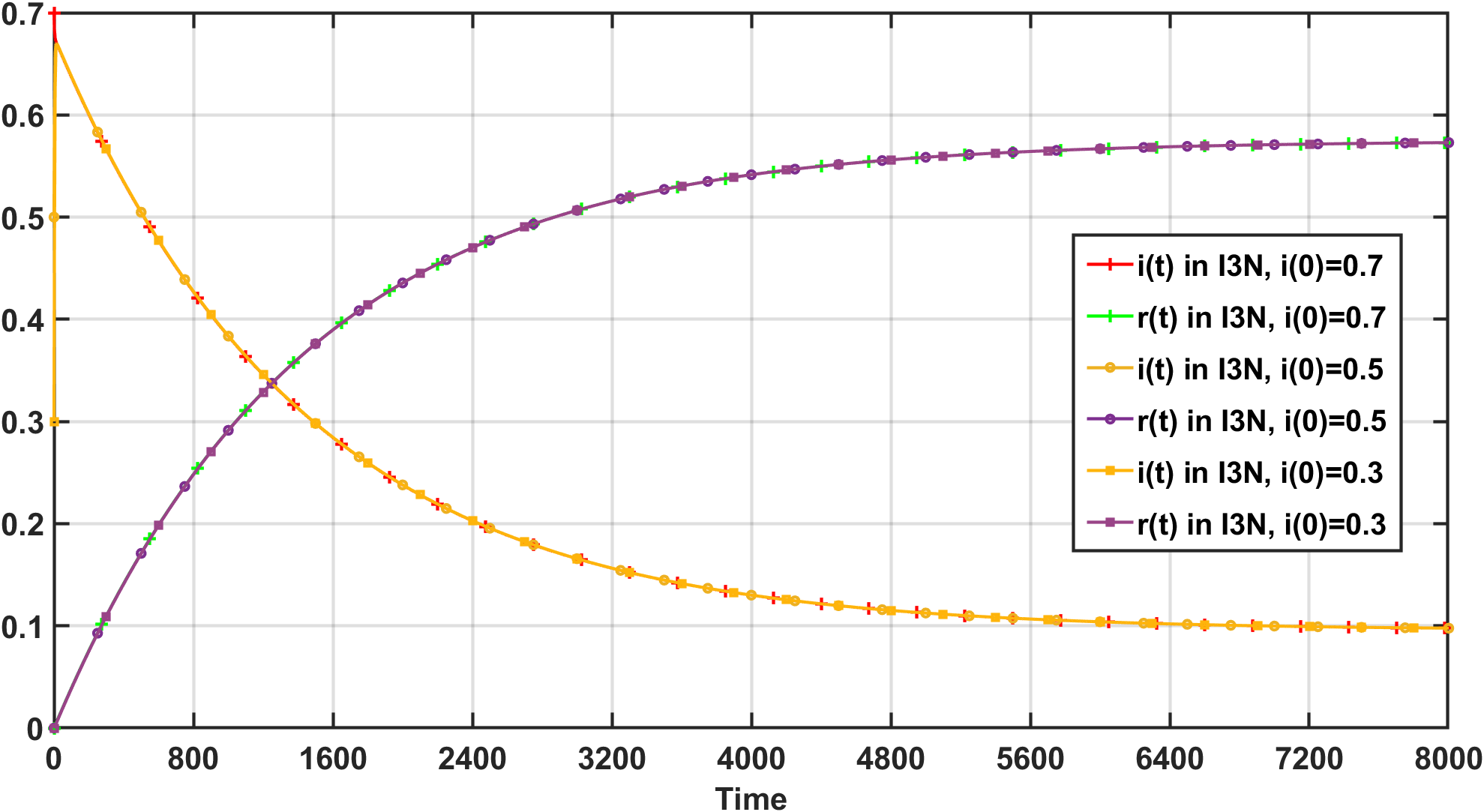
Figure 1: Trajectory settles to $(i^{*},r^{*})$

IV-B Increasing Behavioral Influence by News (IBIN)

When an individual reads news about the epidemic, the response can depend on the infection level. For example, posts that promote mask wearing can positively influence individuals by encouraging them to wear masks when the infection level $i(t)$ is high. The same individual may not follow the recommendation when the infection level is small. Similarly, the response to fake news can be different. Thus the behaviors of the individuals can depend on the infection level. Here, we consider a scenario, in which, the population’s interest in news-items is constant, but their behaviors are influenced by the news. Such scenarios can be captured by letting $\eta(i)\equiv 1$ (and $a=0$) and with $\bar{w}(i)=ui$ (linear influence). The constant $u$ is negative when the news-items are predominantly authentic; it is positive otherwise. The consolidated ODE (14) in this scenario is given by:

$$\frac{di}{dt}=i\big{(}\left(\bar{\beta}+ui\right)(1-i-r)-\alpha\big{)},\mbox{ and}\ \frac{dr}{dt}=\left(i\alpha p_{r}-rl_{i}\right).$$ (16)

We have the following result with proof in the Appendix.

Theorem 4

[Limit-Cycle and Reinfections] Consider the consolidated ODE (16) under the IBIN scenario.
(i) When $\bar{\beta}<\alpha$, $(0,0)$ is an LA. Further if $u<\alpha c_{i}^{r}$, we have the disease-free GPA regime with $(0,0)$ as the only limit.
(ii) When $\bar{\beta}>\alpha$, the disease need not be eradicated and,

1. If $u(1-i^{*}-c_{i}^{r}i^{*})\leq\bar{\beta}+l_{i}/{i^{*}}$, we have the CoP regime with possible limits from $\{(0,0),(i^{*},r^{*})\}$ where:

   $$i^{*}=\frac{(u-\bar{\beta}c^{r}_{i})+\sqrt{(\bar{\beta}c^{r}_{i}-u)^{2}+4uc^{r}_{i}(\bar{\beta}-\alpha)}}{2uc^{r}_{i}}\text{ and}\ \ r^{*}=\frac{i^{*}{\alpha}p_{r}}{l_{i}},$$

2. If $u(1-i^{*}-c_{i}^{r}i^{*})>\bar{\beta}+l_{i}/{i^{*}}$ we have the PCo regime, where $(i(t),r(t))$ eventually follows a periodic path or settles to $(0,0)$ or $(i^{*},r^{*})$. $\Box$

Remarks: In the CoP regime, using the well-known Bendixson’s criterion, one can prove the absence of the limit cycles when additionally $\max\{u/2,\alpha\}<{\bar{\beta}}<\alpha+l_{i}.$ In fact, as in I3N case, no limit cycles are observed, and the dynamics converge only to the LA $(i^{*},r^{*})$, in all our numerical studies .

The possibility to eradicate the disease remains the same when interest in the news does not change with infection levels (see Theorems 2 and 4). Disease free state $(0,0)$ is an LA iff $\bar{\beta}<\alpha$, irrespective of whether $u<0$ (i.e., authentic news is predominant) or $u>0$ (i.e., fake news is predominant).

However, if the disease survives, the limit cycles exist when the population-activities are significantly influenced by the news (see Theorem 4 with $u(1-i^{*}-c_{i}^{r}i^{*})>\bar{\beta}+l_{i}/{i^{*}}$). This result explains the waves of infections (see also Fig. 3): a) when people become reckless and if this reckless behavior increases with infection level under the influence of fake news-items $(u>0)$, the infection rises sharply to a high value and soon susceptible sub-population becomes negligible; b) then the infection starts to reduce and some recovered fraction also begins to lose immunity; however, c) once the susceptible sub-population reaches a reasonable level, the infection rises sharply, again due to people’s reckless activities induced by circulating fake news-items.

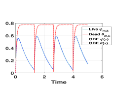
Figure 2: Limit Cycle: News propagation process

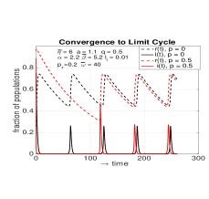
Figure 3: Limit Cycle: Consolidated process. IBIN and I3N&BIN with $u(1-i^{*}-c_{i}^{r}i^{*})>\bar{\beta}+l_{i}/{i^{*}}$

IV-C Increased Interest and Behavioral Influence (IBIN$\&$I3N)

We now consider a scenario in which the population seeks news more proactively and its behavior is also influenced by the news when the infection level increases. The consolidated ODE (14) for this case takes the following form:

$$\frac{di}{dt}=i\left(\left(\bar{\beta}+({\bar{w}}+{u}i)\frac{\bar{\eta}(pi+q)}{a\bar{\eta}(pi+q)+1}\right)(1-i-r)-\alpha\right).$$

One can have limit points as well as limit cycles as in the IBIN case. We consider one such example in Fig. 3, where we further illustrate the differences between IBIN ($p=0$) and IBIN$\&$I3N ($p=0.5$) scenarios, when $\bar{\eta}_{{}_{IBIN\&I3N}}=\bar{\eta}_{{}_{IBIN}}q=\bar{\eta}$ and when ${\bar{w}}_{{}_{IBIN\&I3N}}={\bar{w}}{\bar{\eta}}/(a{\bar{\eta}}+1)$. When the rest of the parameters are the same, both models converge to the same limit cycle. In other words, the asymptotic outcome is not dependent on whether people consume content with an increased interest or not, once the parameters are balanced appropriately.

V Numerical Experiments

In this section, we utilize the historical Twitter and infection datasets of COVID-19 to validate the relationships between the news and epidemic propagation. The real-life COVID-19 situation changes over time and is non-stationary. Building on the proposed framework, we first use the dynamics of the I3N scenario to mimic the trajectory of the COVID-19 infection level from Jan. 1, 2020 to March 15, 2022. We inject authentic or fake news-items with different influence factors at discrete times and obtain the trajectory of influence factors $\{\bar{w}\}$. Let $\bar{\eta}=10$, $p=0.7,q=0.2,a=1.2$, $\bar{\beta}=0.0002,\alpha=0.0001,i(0)=0.00001,p_{r}=0.2,l_{i}=0.01.$ Fig. 4(a) shows that we successfully imitate the historical infection levels. Fig. 4(b) illustrates the influence factors of the news injected at different times.

From Fig. 4(a), we observe that the COVID-19 epidemic propagates with a slow start from Jan. 15, 2020, to March 10, 2020. Then, COVID-19 bursts, and the infection level increases faster. It spawns a large amount of epidemic-related news. Due to the abrupt spreading of the epidemic and the nature of the panic-stricken population, many news-items are fake and produce a significant influence on the epidemic during the period from March 10, 2020, to May 1, 2020, in Fig. 4(b). Once the infection level increases to a notable level, public health agencies make efforts to spread authentic news, including advertising the precautionary measures and reporting the epidemic situation. Authentic news helps reduce the growth rate of the epidemic and produces a negative influence factor on the epidemic. The competition between fake and authentic news lasts for multiple cycles, shown in the time range from May 1, 2020, to Jan. 10, 2021, in Fig. 4(b). After the authentic news dominates for the period from Jan. 10, 2021, to Nov. 10, 2021, in Fig. 4(b), the public becomes accustomed to the epidemic and ignores the protective measures, rekindling the wide propagation of the epidemic and further producing more fake news in the following period from Nov. 10, 2021, to Jan. 1, 2022. The step-wise behavior of the influence depicted in Fig. 4(b) also implies a time-scale separation between the dynamics of the epidemics and the news spreading.

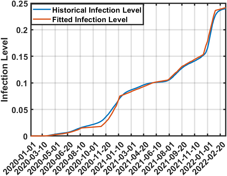
(a) Historical and fitted infection levels

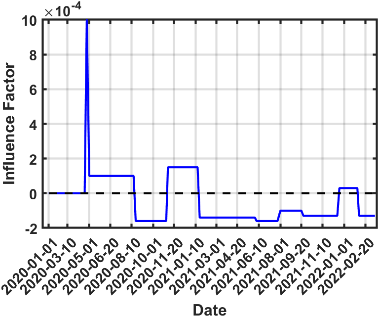
(b) Influence factors by fitting

Figure 4: Total cases versus time: Fitting the historical COVID datasets

We analyze the COVID-related Twitter datasets from Sept. 1, 2020, to Feb. 1, 2021, and obtain the percentage of fake news using a BERT-based approach to corroborate the results on the interplay between the epidemic and fake news. Fig. 5 shows that the percentage of fake news on Twitter is positively correlated with the historical infection rate. The red stars indicate the percentage of fake news on Twitter at discrete time points. The blue line shows the historical infection rate. When the epidemic becomes severer, it generates public panic and promotes the spreading of fake news. Hence, the percentage of fake news on Twitter increases. However, when the epidemic becomes less aggressive, the percentage of fake news decreases.

The understanding of the integrated dynamics enables a short-range prediction despite the non-stationarity in the long run.

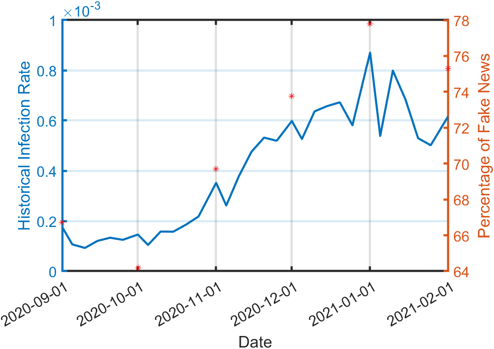
Figure 5: Relationship between the historical infection rate and the percentage of fake news on Twitter. Red stars indicate the percentage of fake news on Twitter and the blue line shows the historical infection rate.

VI Conclusions

In this work, we have presented a two-timescale integrative epidemic model that consolidates the propagation of online social network (OSN) news-items into the compartmental epidemic models; the aim is to study the impact of fake news on the spread of infectious disease. We have analyzed the equilibrium behavior of the coupled dynamic system under different behavioral responses to fake news. We found a periodic pattern of the epidemic when the behavioral response is linearly dependent on the infection level. Our model explains multiple waves of infection and reinfection as seen in the COVID-19 pandemic. We use Twitter and COVID-19 datasets to validate the proposed model. Posting appropriate authentic information can help eradicate the severe spreading of the disease. Misinformation can prolong the epidemic. The successful fitting of the proposed model with the historic COVID-19 dataset shows that the incorporation of human behaviors into the epidemic model provides a promising approach to predicting the trends of the epidemic processes and evaluating public health policies. Motivated by this observation, our future work would focus on the optimal design of intervention mechanisms and policies to mitigate the impact of the pandemic.

We have witnessed many pandemic diseases in the past (including COVID-19), and they exhibit natural period behavior due to the time-varying characteristics of the new mutants. However, the existence of OSNs which facilitate the rapid transfer of information across the globe in the current pandemic has a different impact and the goal of the paper is to capture this aspect. More precisely, the paper proves the existence of infections and reinfections even without the changes in the characteristics of the mutants, which are predominately influenced by the circulating information.

Appendix

Proof of Theorem 1: We consider the general system, (II), where assumptions A.1 and A.2 are satisfied. We show that the equations given by (II) can be approximated by the solution of the ODE (6). We prove this result using [10, Theorem 9, pp. 232].

Assumption required by [10, Theorem 9, pp. 232] To this end, we need to show that the relevant assumptions are satisfied, which are reproduced below as B.1-B.4, in our notations. Consider a stochastic iterative scheme of the type:

$$\phi_{k+1}=\phi_{k}+\epsilon H(\xi_{k+1},\phi_{k}).$$ (17)

If the above scheme satisfies B.1-B.4, then [10, Theorem 9, pp. 232] is applicable.

1. There exists a family ${P_{\phi}}$ of transition probabilities ${P_{\phi}(\xi,A)}$ such that, for any Borel subset $A$, we have

   $$P[\xi_{n+1}\in A\mid\mathcal{F}_{n}]=P_{\phi_{n}}(\xi_{n},A),$$ (18)

   where $\mathcal{F}_{n}=\sigma(\phi_{0},\xi_{0},\xi_{1},\dots,\xi_{n})$ is a sigma-algebra. This in turn implies that the tuple $(\xi_{k},\phi_{k})$ forms a Markov chain.
   

2. For any compact subset $Q$ of $D$, there exist constants $C_{1},q_{1}$ such that for all $\phi\in Q$ we have

   $$\|H(\xi,\phi)\|\leq C_{1}(1+|\xi|^{q_{1}}).$$ (19)

3. There exists a function $h_{1}$ on $D$, and for each $\phi\in D$ a function $\nu_{\phi}(\cdot)$ such that

   1. $h_{1}$ is locally Lipschitz on $D$.

   2. $(I-P_{\phi})\nu_{\phi}(\xi)=H(\xi,\phi)-h_{1}(\phi)$, where $I$ is the identity matrix of the same order as the one of $P_{\phi}$.

   3. For all compact subsets $Q$ of $D$, there exist constants $C_{2},C_{3},q_{2},q_{3}$ and $\lambda\in[0.5,1]$, such that for all $\phi,\phi^{\prime}\in Q$, following is true:

      1. $\|\nu_{\phi}(\xi)\|\leq C_{2}(1+|\xi|^{q_{2}})$,

      2. $\|P_{\phi}\nu_{\phi}(\xi)-P_{\phi}^{\prime}\nu_{\phi}^{\prime}(\xi)\|\leq C_{3}(1+|\xi|^{q_{3}})\|\phi-\phi^{\prime}\|^{\lambda}.$

4. For any compact set $Q$ in $D$ and for any $q>0$, there exists a $\mu_{q}(Q)<\infty$, such that for all n and $\xi,\phi\in R^{d}$, following is true:

   $$E_{\xi,\phi}\{I(\phi_{k},\xi_{k}\in Q,k\leq n)(1+\|\xi_{n+1}\|^{q})\}$$ (20)

   $$\leq\mu_{q}(Q)(1+\|\xi_{n}\|^{q}),$$

   where $E_{\xi,\phi}$ represents the expectation taken with initial conditions $(\xi_{0},\phi_{0})=(\xi,\phi)$.

Assumptions : We now prove that the above assumptions are satisfied by (II). First observe that (II) has the same form as in (17), with $\phi=[\psi,\theta]^{T}$ and,

$$H(\xi,\phi)=\begin{bmatrix}\mathcal{J}_{\phi}(\xi-\theta)+(1-\mathcal{J}_{\phi})(-C\theta)\\ \mathcal{J}_{\phi}(\xi-\psi-1)+(1-\mathcal{J}_{\phi})(-\psi)\end{bmatrix}.$$ (21)

We now prove the required assumptions one after the other.

1. The offsprings $\xi_{k+1}$ depend only upon the total population $\theta_{k}$ and hence assumption B.1 is satisfied with

   $$P_{\phi_{n}}(\xi_{n},A) = Q_{\theta_{n}}(A)\mbox{, where,}$$

   $$\ Q_{\theta_{n}}(A) := P(\xi_{n+1}\in A|\theta_{n}).$$

2. It is direct from (21) that for any compact $Q$

   $$\|H(\xi,\phi)\|\leq\sup_{\phi\in Q}\|\phi\|(1+|\xi|)$$ (22)

   B.2 is satisfied with $q_{1}=1$ and $C_{1}=\sup_{\phi\in Q}||\phi||$ .

3. We will show that assumption B.3 is satisfying by setting $\nu_{\phi}(\xi):=H(\xi,\phi)$ and

   $$h_{1}(\phi) := (P_{\phi})\nu_{\phi}(\xi)\mbox{, where }$$

   $$(P_{\phi})\nu_{\phi}(\xi) = \int H(y,\phi)(Q_{\phi})dy,$$

   Observe that under A.1-2, we have:

   $$h_{1}(\phi)=\begin{bmatrix}\mathcal{J}_{\phi}(\mathcal{M}(\theta)-\theta)+(1-\mathcal{J}_{\phi})(-C\theta)\\ \mathcal{J}_{\phi}(\mathcal{M}(\theta)-1-\psi)+(1-\mathcal{J}_{\phi})(-\psi)\end{bmatrix}.$$ (23)

   We will now prove all the sub-assumptions B.3.a-c in the following:

   1. From equation (23), under A.2, we have:

      $$|h_{1}(\phi)-h_{1}(\phi^{\prime})|$$

      $$\leq(C+1)|\theta-\theta^{\prime}|+2|\psi-\psi^{\prime}|+|\mathcal{M}(\theta)-\mathcal{M}(\theta^{\prime})|$$

      $$\stackrel{{\scriptstyle a}}{{\leq}}(C+1+2\rho)|\theta-\theta^{\prime}|+2|\psi-\psi^{\prime}|$$

      $$\leq D|\phi-\phi^{\prime}|,\mbox{ with }D:=\max\{C+1+2\rho,2\},$$

      where ‘a’ hold true as $\lambda\leq 1$. Thus, $h_{1}$ is locally Lipschitz.

   2. The definitions of $h_{1}(\phi)$ and $H(\xi,\phi)$ make this obvious.

   3. 1. This proved along with B.2, as

         $$\nu_{\phi}(\xi)=H(\xi,\phi).$$

      2. From (iiia) and definition of $h_{1}(\phi)$, this assumption is satisfied.

4. For proving B.4, consider any compact $Q$, then we can upper bound the LHS of (20) as below:

   $$E_{\xi,\phi}\{I(\phi_{k},\xi_{k}\in Q,k\leq n)(1+\|\xi_{n+1}\|^{q})\}$$

   $$\leq E_{\xi,\phi}\{I(\phi_{n},\xi_{n}\in Q)(1+\|\xi_{n+1}\|^{q})\}$$

   $$\leq\sup_{\phi\in Q}\int(1+y^{q})Q(\phi,dy)$$

   $$=\sup_{\phi\in Q}E[1+\xi_{n+1}^{q}|\theta_{n}=\theta]$$

   $$\stackrel{{\scriptstyle a}}{{\leq}}1+\rho^{q}$$

   $$\leq(1+\rho^{q})(1+||\xi_{n}||^{q})$$

   for any $q>0$, where equality ‘a’ follows from assumption A.2. Then, B.4 hold with $\mu_{q}(Q):=1+\rho^{q}$.

Now, using [10, Theorem 9, pp. 232], the result is proved. $\Box$

ODE Solution and the Derivation of (9): We consider the system (II) and the corresponding ODEs are given in (6).

Say, we start in regime $\mathcal{R}^{1}$, and say with $\psi(0)=\delta_{\psi}$ and some $\theta(0)>\delta_{\theta}$. Then, the solution is given by

$$\psi(\tau)=\delta_{\psi}e^{-\tau}\mbox{ \normalsize and }\theta(\tau)=\theta(0)e^{-C\tau}.$$

And then, there exists a time epoch (say $\tau_{1}=\nu_{1}$) such that

$$\theta(\nu_{1})=\delta_{\theta}\ \ (\mbox{\normalsize say }\theta_{01})\mbox{ \normalsize and let }\psi(\nu_{1}):=\psi_{01}.$$

Regime ${\cal R}^{2}$: Let $\Delta=a\eta+1$. The solution after time epoch $\tau_{1}$, with initial conditions $\phi(\tau_{1})=(\psi_{01},\delta_{\theta})$, is given by:

$$\psi(\tau+\tau_{1}) =\Delta\theta(\tau+\tau_{1})+(\psi_{01}-\delta_{\theta}\Delta+a\eta^{2}+1)e^{-\tau}-a\eta^{2}-1,$$

$$\theta(\tau+\tau_{1}) =\left(\delta_{\theta}-\frac{\eta}{\Delta}\right)e^{-\Delta\tau}+\frac{\eta}{\Delta}.$$

Then, there exists epoch $\tau_{2}=\nu_{2}+\tau_{1}$, with $\nu_{2}>0$, such that

$$\psi(\tau_{2}) = \delta_{\psi}=:\ \psi_{02}\mbox{ \normalsize and }$$

$$\theta(\tau_{2}) = \left(\delta_{\theta}-\frac{\eta}{\Delta}\right)e^{-\Delta\nu_{2}}+\frac{\eta}{\Delta}=:\theta_{02}.$$

This completes $1$-st cycle, i.e., $L_{C_{1}}$. Now it goes back to regime 1, with initial conditions $\phi(\tau_{2})=(\psi_{02},\theta_{02})$ and continues this pattern. We can construct series of time epochs $\tau_{i}$ with appropriate initial conditions, constructed from the terminal conditions of previous regimes.

This process continues and we arrive at a periodic asymptotic solution. This limit can be specified if the initial/terminal conditions can be identified by solving the following fixed-point equations (recall $\Delta=a\eta+1$):

$$\theta_{02}^{*}=\theta(\nu_{2}^{*}) = \left(\delta_{\theta}-\frac{\eta}{\Delta}\right)e^{-\Delta\nu_{2}^{*}}+\frac{\eta}{\Delta},$$

$$\psi_{01}^{*}=\psi(\nu_{1}^{*}) = \delta_{\psi}e^{-\nu_{1}^{*}}\mbox{, where, }\ \theta_{02}^{*}e^{-C\nu_{1}^{*}}\ =\ \delta_{\theta}\mbox{ and }$$

$$\Delta\theta_{02}^{*}+(\psi^{*}_{01}-\delta_{\theta}\Delta+a\eta^{2}+1)e^{-\nu_{2}^{*}}-a\eta^{2}-1=\delta_{\psi}.$$

At the limit and in Regime 2, we have for any $\tau\leq\nu_{2}^{*}$

$$\theta(\tau+\tau_{\infty}) = \left(\delta_{\theta}-\frac{\eta}{\Delta}\right)e^{-\Delta\tau}+\frac{\eta}{\Delta}.$$

When $\nu_{2}^{*}$ is sufficiently large, one can approximate $\theta_{02}^{*}\approx\eta/\Delta.$ Under this approximation, the fixed-point equations are solved by:

$$\theta_{02}^{*}\approx\frac{\eta}{\Delta},\ \ \ \nu_{1}^{*}=\frac{-1}{C}\ln\left(\frac{\Delta\delta_{\theta}}{\eta}\right),\ \psi_{01}^{*}=\delta_{\psi}e^{-\nu_{1}^{*}}\approx\delta_{\psi}\left(\frac{\Delta\delta_{\theta}}{\eta}\right)^{1/C}.$$

Thus, the limit in (9) equals

$${\theta}_{\infty}^{*}(\eta):=\lim_{k\to\infty}\max_{\tau^{\prime}\in L_{C_{k}}}\theta(\tau^{\prime})=\theta_{02}^{*}\approx\frac{\eta}{a\eta+1}.$$ (25)

Appendix: Proofs related to Epidemic-ODE

It is easy to verify that global unique solutions exist for all ODEs considered, as the Right-Hand Sides (RHS) are Lipschitz continuous. We first show that for any initial condition (i.c.) in $B^{(2)}$, the solution remains in ${B}^{(2)}$:

Lemma 1

Consider the two-dimensional ODE defined in (14). Consider any i.c. $(i_{0},r_{0})\in{B}^{(2)}$, then the unique solution $(i(t),r(t))\in B^{(2)}$ for all $t$.

Proof: We will show that the flow of the ODE on the boundary of $B^{(2)}$ is either inwards or on the boundary (see Fig. 6). This provides the required result by Nagumo’s theorem [13], which then says that any trajectory started inside region $B^{(2)}$ will remain in $B^{(2)}$.

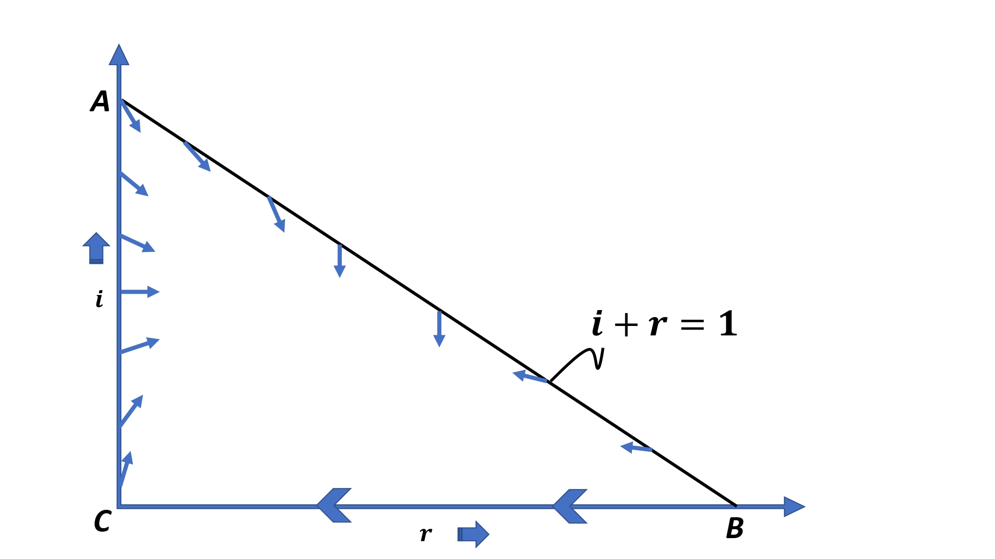
Figure 6: ODE Trajectory

Consider any $(r,i)\in\partial B^{(2)}$. When the boundary point is $(r,0)$ (i.e., on $r$-axis as shown in figure), then clearly from ODE (14), $di/dt=0$ while $dr/dt<0$, so the flow is directed towards $(0,0)$ and along the boundary line $BC$. Now, for any point $(0,i)$ on the boundary $AC$, again from ODE (14), $dr/dt>0$ and depending upon $\beta(i)$, the ODE flow is either upwards and towards right or downwards and towards right (as shown in figure 6); in either case the flow is into $B^{(2)}$. At the corner point $A$, the slope of flow is $\frac{di}{dr}=\frac{-\alpha i}{i\alpha p_{r}}=\frac{-1}{p_{r}},$ whose magnitude is greater than one (because $p_{r}$ is the fraction of recovered that get immunized, and hence $p_{r}<1$), which is hence ${di}/{dr}$ is smaller than the slope of $AB$ (as the slope of line $i+r=1$ is $-1$). So, flow at $A$ is also into $B^{(2)}$. Now consider any point $(r,i)$ on line $AB$; here $i+r=1$ and hence the slope of the flow, $\frac{di}{dr}=\frac{-\alpha i}{i(\alpha p_{r}+l_{i})-l_{i}},$ which is increasing with $i$ and hence ${di}/{dr}$ for any $(r,i)$ on $AB$ is less than that at $A$, i.e., ${di}/{dr}<-1/p_{r}$. Thus the flow is inward on $AB$ also. Proof follows by Nagumo’s theorem [13]. $\Box$

Proof of Theorem 2: For the ODE (10), (0,0) is an equilibrium point, we have another equilibrium point, $(i^{*},r^{*})$,

$$i^{*}=\frac{\bar{\beta}-\alpha}{\bar{\beta}(1+\frac{\alpha p_{r}}{l_{i}})}\ \mbox{ and }r^{*}\ =\ \frac{i^{*}\alpha p_{r}}{l_{i}}.$$ (26)

Furthermore, the Jacobian matrix at any $(i,r)$ is:

$$J(i,r)=\begin{bmatrix}\bar{\beta}(1-i-r)-\alpha-\bar{\beta}i&-i\bar{\beta}\\ \alpha p_{r}&-l_{i}\end{bmatrix}.$$

Matrix $J(0,0)$ is negative definite and (0,0) is LA iff $\bar{\beta}<\alpha$.

Case with $\bar{\beta}<\alpha$: For this case, from (26), $i^{*}<0$ for the non-zero equilibrium point. Thus there is only one equilibrium point in ${B}^{(2)}$, which is $(0,0)$. Further, there cannot be a limit cycle inside $B^{(2)}$, as it has to enclose $(0,0)$ (and not touch it), see [14], and, as any trajectory (with i.c., in $B^{(2)}$) is trapped inside $B^{(2)}$ by Lemma 1. Thus by Poincaré–Bendixson theorem (e.g., [14]), the limit set of any trajectory staring in $B^{(2)}$ is $\{(0,0)\}$, which implies that $(0,0)$ is a global attractor (as it is a local attractor).

Case $\bar{\beta}>\alpha$: The Jacobian matrix, $J(i^{*},r^{*})=\begin{bmatrix}-\bar{\beta}i^{*}&-\bar{\beta}i^{*}\\ \alpha p_{r}&-l_{i},\end{bmatrix},$ is negative definite (use minors). Thus $(i^{*},r^{*})$ is an LA.

In Lemma 3, we have constructed a bounded region (e.g., ABCD in left sub-figure, Fig. 7), call it ${\cal R}$, with flow inwards or on boundary. On applying Nagumo’s theorem [13], any trajectory started inside region ${\cal R}$ will remain in ${\cal R}$. Further, using the Bendixson criterion (e.g., [12]), there will be no limit cycle inside the region ${\cal R}$ because of (3) in Lemma 3.

Then, by Poincaré–Bendixson (PB) theorem (e.g., [14, Theorem 1.8]), the ODE trajectory starting in ${\cal R}$ has a unique limit point, and as the limit point is an LA, the trajectory converges to $(i^{*},r^{*})$. Now, by the critical point criterion ([14]), any closed orbit has a critical point (which is not a saddle point) in its interior. That means $B^{(2)}/{\cal R}$ does not contain any limit cycle, because any such limit cycle should intersect the region ${\cal R}$ as it has to enclose $(i^{*},r^{*})$, which contradicts the fact that all points on or inside ${\cal R}$ are attracted toward $(i^{*},r^{*})$. This completes the proof. $\Box$

Proof of Theorem 3: For ODE (15), again $(0,0)$ is an equilibrium point and the other equilibrium points are:

$$i^{*}=\frac{-c_{b}\pm\sqrt{(c_{b})^{2}-4c_{a}c_{c}}}{2c_{a}},\ r^{*}=\frac{\alpha p_{r}}{l_{i}}i^{*}.$$ (27)

We now identify the ones in $B^{(2)}$ (equivalently $i^{*}\in[0,1/c_{i}^{r}]$, for $c_{i}^{r}:=1+\alpha p_{r}/l_{i}$) and further identify if they are attractors. Consider the corresponding Jacobian matrices:

$$J(i^{*},r^{*})=\begin{bmatrix}i^{*}(2i^{*}c_{a}+c_{b})&-i^{*}\bar{\beta}\\ \alpha p_{r}&-l_{i}\end{bmatrix}\mbox{, }J(0,0)=\begin{bmatrix}\beta_{0}-{\alpha}&0\\ \alpha p_{r}&-l_{i}\end{bmatrix}.$$

Case I, when $\beta_{0}-{\alpha}<0$: Begin with sub-case ${\bar{w}}<0$ and define, $L(i)=\eta(pi+q)$. If ${\bar{\beta}}+{\bar{w}}\frac{L(i)}{aL(i)+1}<0$, then from ODE (15), we clearly have:

$$\frac{di}{dt}<-i\alpha<-i\min\{\alpha,\alpha-\beta_{0}\}.$$

On the other hand, when ${\bar{\beta}}+{\bar{w}}\frac{L(i)}{aL(i)+1}\geq 0$, we have

$$\frac{di}{dt} \leq i\left({\bar{\beta}}+{\bar{w}}\frac{L(i)}{aL(i)+1}-\alpha\right)$$

$$\stackrel{{\scriptstyle a}}{{\leq}} i(\beta_{0}-\alpha)\ \ <\ -i\min\{\alpha,\alpha-\beta_{0}\}.$$

and the inequality ‘$a$’ holds because the function $i\mapsto L(i)/(aL(i)+1)$ is increasing and $\bar{w}<0$. Thus in all, with ${\bar{w}}<0$, we have

$$\frac{di}{dt} \leq -i\min\{\alpha,\alpha-\beta_{0}\}.$$

By standard results in ODEs, we have that (also given as [7, Lemma 6]), $i(t)\leq i_{0}\exp\left({-\min\{\alpha,\alpha-\beta_{0}\}t}\right)\to 0$. Also $i(t)\geq 0$ by Lemma 1. Hence, $i(t)\to 0$ and it is simple to show that $(0,0)$ is a global attractor on $B^{(2)}$, when ${\bar{w}}<0$ (see r-ODE in (14)).

Now, consider the sub-case with $\beta_{0}<\alpha$, and ${\bar{w}}>0$, but $\beta a+{\bar{w}}-\alpha a<0$; then one can upper bound the $i$-ODE as:

$$\frac{di}{dt}\leq i\left(\beta+\frac{{\bar{w}}}{a}-\alpha\right)=\frac{i}{a}(\beta a+{\bar{w}}-\alpha a)<0,$$

and hence $(i(t),r(t))\to(0,0)$, as before, for any i.c.

Case II, with $\beta_{0}-{\alpha}>0$: Define the function

$$p_{1}(i)=c_{a}i^{2}+c_{b}i+c_{c},\mbox{ for }i\in[0,1/c_{i}^{r}].$$

Then, $p_{1}(0)=(\beta_{0}-{\alpha})(a\bar{\eta}q+1)>0$ and, $p_{1}(1/c_{i}^{r})=-\alpha<0$. Thus, by continuity, there exists a unique zero of $p_{1}(i)\in(0,1/c_{i}^{r}]$, and is one of the two values in (27).

The square root term will be $\sqrt{c_{b}^{2}-4c_{a}c_{c}}>\mbox{ or }<|c_{b}|$, when $c_{a}$ is positive or negative, respectively. In both cases, the negative sign of square root term leads to the required root, irrespective of $c_{b}>0$ or $c_{b}<0$. Thus,

$$i^{*}=\frac{-c_{b}-\sqrt{(c_{b})^{2}-4c_{a}c_{c}}}{2c_{a}},\ r^{*}=\frac{\alpha p_{r}}{l_{i}}i^{*}.$$

The corresponding Jacobian matrix $J(i^{*},r^{*})$ is negative definite, making $(i^{*},r^{*})$ an LA because

$$2i^{*}c_{a}+c_{b}=-\left(c_{b}+\sqrt{c_{b}^{2}-4c_{a}c_{c}}\right)+c_{b}=-\sqrt{c_{b}^{2}-4c_{a}c_{c}}<0.$$

The proof now follows by Lemma 1 and PB theorem. $\Box$

Proof of Theorem 4: For ODE (16) using Jacobian matrix, $(0,0)$ is an LA iff $\bar{\beta}<\alpha$. The possible nonzero equilibrium points are given by:

$$i^{*}=\frac{(u-\bar{\beta}c^{r}_{i})\pm\sqrt{(\bar{\beta}c^{r}_{i}-u)^{2}+4uc^{r}_{i}(\bar{\beta}-\alpha)}}{2uc^{r}_{i}},\ r^{*}=\frac{i^{*}\alpha p_{r}}{l_{i}}.$$ (28)

When ${\bar{\beta}}<\alpha$ and $u<\alpha c_{i}^{r}$, using simple algebra one can show that these non-zero equilibrium points will not lie in interval $[0,1/c^{r}_{i}]$. Thus, by PB theorem the limit set with respect to any i.c., inside $B^{2}$, is $\{(0,0)\}$. Further since $\{(0,0)\}$ is an LA, the limit point becomes the limit and hence the global attractor.

When $\bar{\beta}>\alpha$, Define the function

$$p_{2}(i)=\left(\bar{\beta}+ui\right)(1-c_{i}^{r}i)-\alpha,\mbox{ for }i\in[0,1/c_{i}^{r}].$$

$p_{2}(0)=(\bar{\beta}-{\alpha})>0$ and $p_{2}(1/c_{i}^{r})=-{\alpha}<0$. Thus by continuity, only one non-zero root given by (28) lies in $[0,1/c_{i}^{r}]$.

On following similar arguments as before, $\sqrt{(\bar{\beta}c^{r}_{i}-u)^{2}+4uc^{r}_{i}(\bar{\beta}-\alpha)}>\mbox{ or }<|u-\bar{\beta}c^{r}_{i}|$, if $u$ is positive or negative respectively. So the only root with positive sign of square root will work, irrespective of the sign of $(u-\bar{\beta}c^{r}_{i})$.

Hence, in both cases,

$$i^{*}=\frac{(u-\bar{\beta}c^{r}_{i})+\sqrt{(\bar{\beta}c^{r}_{i}-u)^{2}+4uc^{r}_{i}(\bar{\beta}-\alpha)}}{2uc^{r}_{i}},\ r^{*}=\frac{i^{*}\alpha p_{r}}{l_{i}}.$$

lies in $B^{(2)}$. Now, at $(i^{*},r^{*})$, the Jacobian matrix is:

$$J(i^{*},r^{*})=\begin{bmatrix}i^{*}(u(1-i^{*}-r^{*})-\bar{\beta}-ui^{*})&-i^{*}(\bar{\beta}+ui^{*})\\ \alpha p_{r}&-l_{i}\end{bmatrix}.$$ (29)

The product of eigenvalues of (29) is greater than zero by Lemma 2, and hence $(i^{*},r^{*})$ is either a source or sink. Thus it is a negative definite iff $u(1-c_{i}^{r}i^{*})\leq{\bar{\beta}}+ui^{*}+l_{i}/i^{*},$ otherwise, $(i^{*},r^{*})$ will be a source. Thus part (ii).a follows by PB theorem, as $(i^{*},r^{*})$ is now an LA.

For part (ii).b, $(i^{*},r^{*})$ is unstable. There cannot be a closed orbit (or limit cycle) that just encloses $(0,0)$ by the critical point criterion (e.g., [14]), as $(0,0)$ is a saddle point. Further, the trajectory starting from $(r,0)$ in $B^{(2)}$, will converge to $(0,0)$. We need to understand the remaining trajectories. The rest of the theorem follows from PB theorem, as $(i^{*},r^{*})$ is the only other equilibrium point, and it is not a saddle point; thus a trajectory in $B^{(2)}$ approaches a limit cycle enclosing $(i^{*},r^{*})$, or approaches one of the two equilibrium points. $\Box$

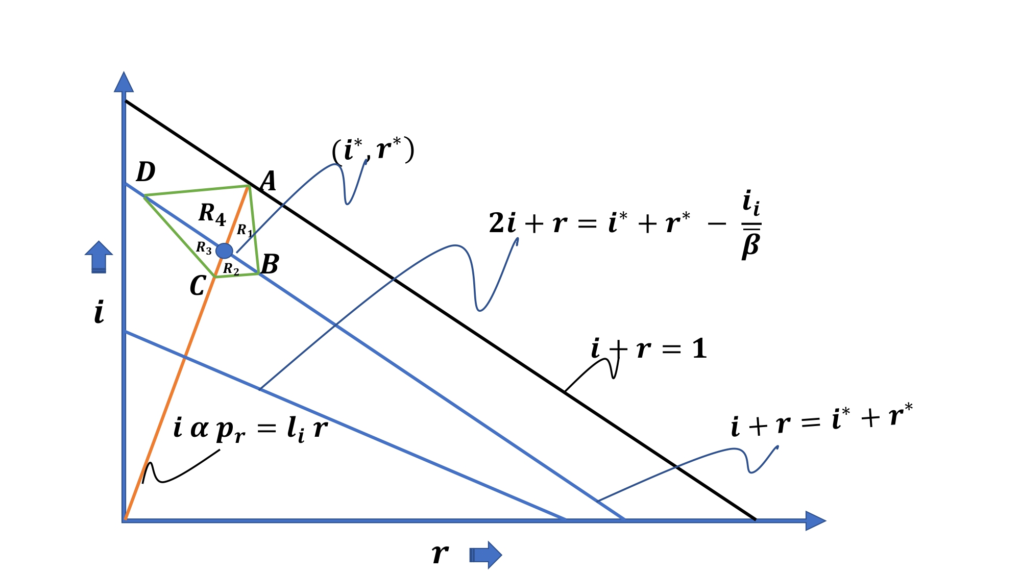
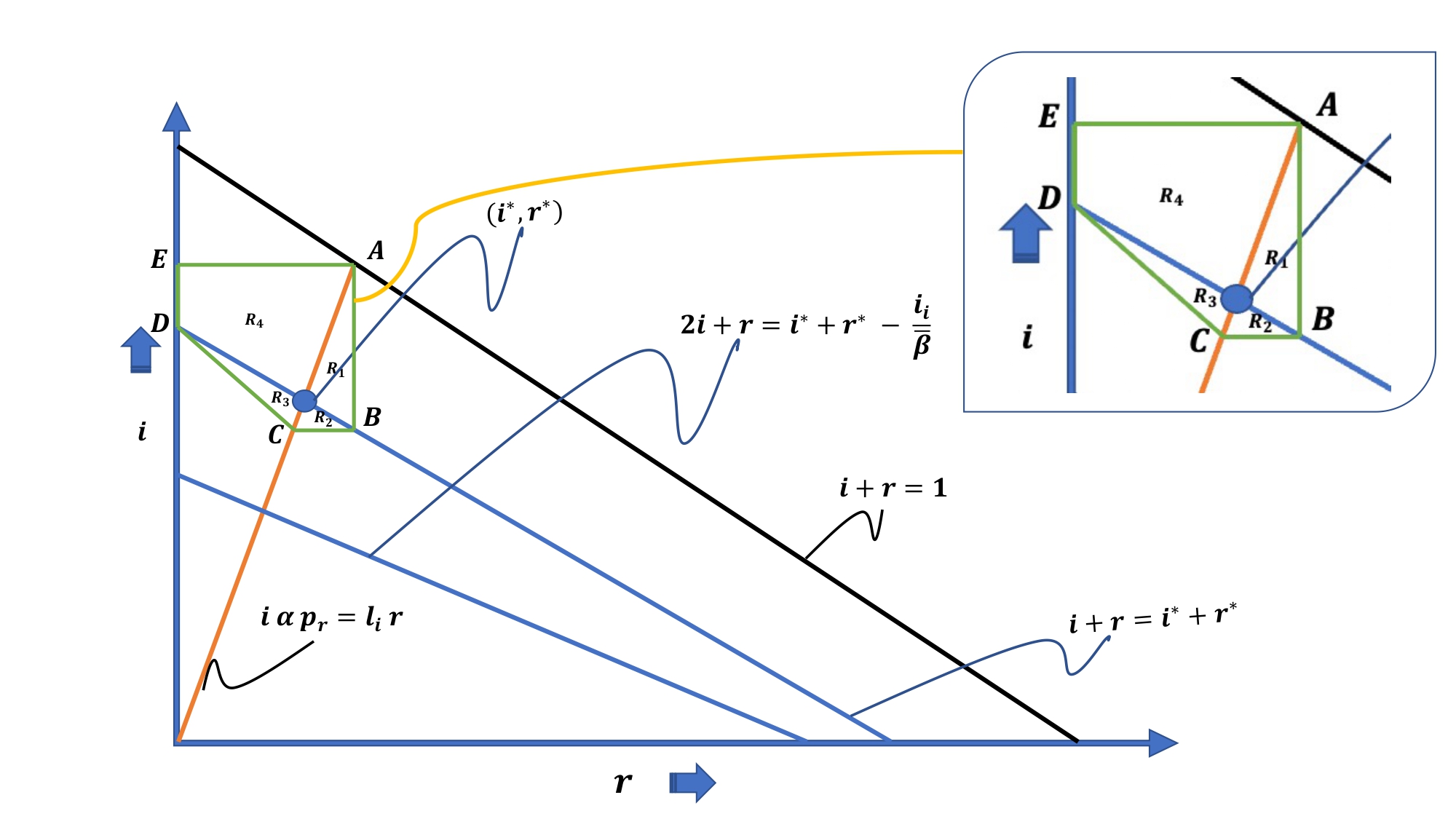
Figure 7: Left: $\alpha+l_{i}<\bar{\beta}$, $\bar{\beta}<1+\frac{l_{i}}{\alpha p_{r}}$,   Right: $\alpha+l_{i}<\bar{\beta}$, $\bar{\beta}>1+\frac{l_{i}}{\alpha p_{r}}$

Lemma 2

The product term of Jacobian matrix (29) is positive.

Proof: The product term is

$$i^{*}\left(-\left(\frac{u\alpha}{K}-K\right)l_{i}+K\alpha p_{r}\right)=\frac{i^{*}l_{i}}{K}\left(c_{i}^{r}K^{2}-{u\alpha}\right),$$

where $K:={\bar{\beta}+ui^{*}}$. Now, as $K=\frac{\alpha}{1-i^{*}-r^{*}}>0$, we check the sign of $\left(c_{i}^{r}K^{2}-{u\alpha}\right)$ term only. So, consider

$$4c_{i}^{r}(c_{i}^{r}K^{2}-{u\alpha})$$

$$=\left(2\bar{\beta}c_{i}^{r}+(u-\bar{\beta}c_{i}^{r})+\sqrt{(u+\bar{\beta}c_{i}^{r})^{2}-4\alpha uc_{i}^{r}}\right)^{2}-4\alpha uc_{i}^{r}$$

$$=2(u+\bar{\beta}c_{i}^{r})^{2}-8\alpha uc_{i}^{r}+2(u+\bar{\beta}c_{i}^{r})\sqrt{(u+\bar{\beta}c_{i}^{r})^{2}-4\alpha uc_{i}^{r}},$$

is positive as $(u+\bar{\beta}c_{i}^{r})^{2}>4\alpha uc_{i}^{r}$, because the square root term $(u+\bar{\beta}c_{i}^{r})^{2}-4\alpha uc_{i}^{r}>0$ used for $(i^{*},r^{*})$ definition. Now as $c_{i}^{r}$ is positive, the product term is positive. This completes the proof. $\Box$

Lemma 3

Under the assumptions of Theorem 2.(ii), one can construct a closed, bounded region ${\cal R}\subset B^{(2)}$, touching boundary $\{i+r=1\}\subset\partial(B^{(2)})$ at $A=(b_{*},1-b_{*})\in\partial{\cal R}$, where $b_{*}=l_{i}/(l_{i}+\alpha p_{r})$, such that

$$\pdv{f}{i}+\pdv{g}{r}=-(\bar{\beta}(2i+r-i^{*}-r^{*})+l_{i})\neq 0,\mbox{ where }$$

$$f(i,r)=i\left(\bar{\beta}(1-i-r)-\alpha\right),\mbox{ and, }g(i,r)=i\alpha p_{r}-l_{i}r,$$ (30)

and such that the field $(f,g)$ representing ODE (10) at the boundary $\partial{\cal R}$ is pointing inwards or onto the boundary $\partial{\cal R}$.

Proof of Lemma 3: Here, we will construct a bounded region, such that the field of the ODE on its boundary is either inwards or on the boundary of that bounded region. Then, similar arguments will follow as lemma 1. Further, the region can be constructed in such a way that the line given by

$$\bar{\beta}(2i+r-i^{*}-r^{*})+l_{i}=0,$$ (31)

is outside the region ${\cal R}$ (see Fig. 7). We will have three cases the following:

VI-A Consider the case when $\alpha+l_{i}<\bar{\beta}$ and $\bar{\beta}<1+\frac{l_{i}}{\alpha p_{r}}$

At the corner point $A=\left(\frac{\alpha p_{r}}{\alpha p_{r}+l_{i}},\frac{l_{i}}{\alpha p_{r}+l_{i}}\right)$, the flow is downwards (along line $AB$) as $dr/dt=0$ and $di/dt<0$. Similarly, at corner point $B$, flow is towards left (along line $BC$) as on line $i+r=i^{*}+r^{*}$, ${di}/{dt}=0$ and $dr/dt<0$ is decreasing (as $i\alpha p_{r}<rl_{i}$). Similar arguments will follow for corner points $C$ and $D$. Now, consider any point $(r,i)\mbox{ on }AB$, flow will be inwards as $di/dt<0$ and $dr/dt<0$ are decreasing (because $(r,i)\in\{(r,i);i+r>i^{*}+r^{*}\mbox{ and }i\alpha p_{r}<rl_{i}\}$). Similarly, for any point $(r,i)$ on boundary $BC$, have flow upwards as $i$ is increasing below line $(i+r=i^{*}+r^{*})$ and $r$ is decreasing below line $(i\alpha p_{r}=rl_{i})$. Similar arguments will follow for boundary lines $CD$ and $DA$.

Furthermore, observe that the above arguments only require that $AB$ is vertical ($A$ touching the lines $i+r=1$ and $\alpha p_{r}i=l_{i}r$), both $AD$ and $BC$ are horizontal and CD is then joining the points. Thus one can shift the line $BC$ upward if required to ensure, $C$ does not touch the line given in (31) (observe that $2i+l_{i}/\beta=i$ only when ${\bar{\beta}}<0$, which is not true here, thus there is a gap between lines $i+r=i^{*}+r^{*}$ and the line given in (31)).

VI-B Consider the case when $\alpha+l_{i}<\bar{\beta}$ and $\bar{\beta}>1+\frac{l_{i}}{\alpha p_{r}}$

On following the similar arguments as above, one can prove the trajectory will be confined in the $ABCDE$ region when started from anywhere inside the same region. Further again, the lines $2i+l_{i}/\beta+r=i^{*}+r^{*}$ and $i+r=i^{*}+r^{*}$ have a gap in between because $\beta>0.$

VI-C Consider the case when $\alpha+l_{i}>\bar{\beta}$

In this scenario, by the Bendixson criterion, we don’t have any limit cycle in the $B^{(2)}$ region. And further a bounded region as in previous cases can be constructed,

This completes the proof by applying Nagumo’s theorem [13]. $\Box$

References

- [1] Y. Benkler, R. Faris, and H. Roberts, Network propaganda: Manipulation, disinformation, and radicalization in American politics, 2018.
- [2] S. Kapsikar, I. Saha, K. Agarwal, V. Kavitha, and Q. Zhu, “Controlling fake news by collective tagging: A branching process analysis,” IEEE Control Systems Letters, vol. 5, no. 6, pp. 2108–2113, 2020.
- [3] C. Granell, S. Gómez, and A. Arenas, “Competing spreading processes on multiplex networks: awareness and epidemics,” Physical review E, vol. 90, no. 1, p. 012808, 2014.
- [4] S. Liu, Y. Zhao, and Q. Zhu, “Herd behaviors in epidemics: A dynamics-coupled evolutionary games approach,” Dynamic Games and Applications, pp. 1–31, 2022.
- [5] Y. Huang and Q. Zhu, “Game-theoretic frameworks for epidemic spreading and human decision-making: A review,” Dynamic Games and Applications, pp. 1–42, 2022.
- [6] Q. Zhu, E. Gubar, and E. Altman, “Preface to special issue on dynamic games for modeling and control of epidemics,” Dynamic Games and Applications, pp. 1–6, 2022.
- [7] K. Agarwal and V. Kavitha, “New results in branching processes using stochastic approximation,” arXiv preprint arXiv:2111.14527, 2021.
- [8] A. Khushboo and V. Kavitha, “Saturated total-population dependent branching process and viral markets,” CDC, 2022.
- [9] A. Lahrouz, L. Omari, and D. Kiouach, “Global analysis of a deterministic and stochastic nonlinear sirs epidemic model,” Nonlinear Analysis: Modelling and Control, vol. 16, no. 1, pp. 59–76, 2011.
- [10] A. Benveniste, M. Métivier, and P. Priouret, Adaptive algorithms and stochastic approximations. Springer Science & Business Media, 2012.
- [11] V. Singh, K. Agarwal, V. Kavitha et al., “Evolutionary vaccination games with premature vaccines to combat ongoing deadly pandemic,” in EAI International Conference on Performance Evaluation Methodologies and Tools. Springer, 2021, pp. 185–206.
- [12] F. Verhulst, Nonlinear differential equations and dynamical systems. Springer Science & Business Media, 2006.
- [13] K. Ghorbal and A. Sogokon, “Characterizing positively invariant sets: Inductive and topological methods,” Journal of Symbolic Computation.
- [14] J. J. Palis and W. De Melo, Geometric theory of dynamical systems: an introduction. Springer Science & Business Media, 2012.