Optimal approximation of spherical squares by tensor product quadratic Bézier patches

Abstract

In [1], the author considered the problem of the optimal approximation of symmetric surfaces by biquadratic Bézier patches. Unfortunately, the results therein are incorrect, which is shown in this paper by considering the optimal approximation of spherical squares. A detailed analysis and a numerical algorithm are given, providing the best approximant according to the (simplified) radial error, which differs from the one obtained in [1]. The sphere is then approximated by the continuous spline of two and six tensor product quadratic Bézier patches. It is further shown that the $G^{1}$ smooth spline of six patches approximating the sphere exists, but it is not a good approximation. The problem of an approximation of spherical rectangles is also addressed and numerical examples indicate that several optimal approximants might exist in some cases, making the problem extremely difficult to handle. Finally, numerical examples are provided that confirm theoretical results.

1 Introduction

One of the most important issues of computer-aided geometric design (CAGD) is the approximation of curves and surfaces by simple polynomial-based objects. It is well known that even fundamental geometric objects such as circular arcs or spherical patches do not possess exact polynomial representations. It is thus an interesting and practical issue to find their best polynomial approximants. Much work has been done on the optimal polynomial approximation of circular arcs (see, e.g., [4] and the references therein). However, much less is known about the optimal approximation of spherical patches. The main two classes of the polynomial (or spline) surfaces used in CAGD are triangular patches and tensor product patches. The optimal approximation of equilateral spherical triangles by triangular Bézier patches was studied recently in [5]. Approximation of rational tensor-product biquadratic Bézier surfaces (which also includes the sphere) by polynomial tensor product patches was proposed in [2]. An exact sphere representation by rational S-patches was considered recently in [3]. In [1], the author studied the problem of the best approximation of symmetric surfaces by biquadratic Bézier surfaces. However, we show in this paper that the obtained results are incorrect since the constructed approximants are not optimal even in the spherical case. Our primary purpose is to characterize the optimal polynomial approximant and provide an algorithm for its construction.

The paper is organized as follows. After the introduction in Section 1 some basic preliminaries are explained in Section 2. The detailed analysis of the construction of the best approximant together with a numerical algorithm are given in Section 3. The next section considers $G^{1}$ smooth optimal approximants of the sphere. In Section 5 some basic observations of the approximation of spherical rectangles are provided. Numerical examples are shown in Section 6, and some closing remarks are given in the last section.

2 Preliminaries

Let ${\mathcal{S}}$ be the unit sphere in $\mathbb{R}^{3}$ centered at $\boldsymbol{0}=(0,0,0)$ and let ${\mathcal{R}}$ be the spherical square for which the projection of its vertices along the vector $[0,0,1]^{T}$ are vertices of the square centered at $(0,0)$ with its side equal to $2a$, where $0<a\leq\tfrac{\sqrt{2}}{2}$. Let ${\mathcal{P}}$ be a tensor product quadratic Bézier patch parameterized as

$$\boldsymbol{p}(u,v)=\sum_{i=0}^{2}\sum_{j=0}^{2}B_{i}^{2}(u)B_{j}^{2}(v)\boldsymbol{b}_{ij},\quad u,v\in[-1,1],$$ (1)

where

$$B_{i}^{2}(u)=\sum_{i=0}^{2}\binom{2}{i}\left(\frac{1+u}{2}\right)^{i}\left(\frac{1-u}{2}\right)^{2-i},\quad i=0,1,2,$$

are quadratic Bernstein polynomials parametrized on $[-1,1]$ and $\boldsymbol{b}_{ij}\in\mathbb{R}^{3}$, $i,j=0,1,2$, are the corresponding control points. Our goal is to find the optimal approximation of ${\mathcal{R}}$ by ${\mathcal{P}}$ according to the radial error

$$\max_{(u,v)\in[-1,1]^{2}}\left|\|\boldsymbol{p}(u,v)\|_{2}-1\right|$$

or according to the simplified radial error

$$\max_{(u,v)\in[-1,1]^{2}}\left|f(u,v)\right|,\quad f(u,v)=\|\boldsymbol{p}(u,v)\|_{2}^{2}-1.$$ (2)

Note that the latter one is easier to handle since $f$ is a polynomial function of the coefficients of $\boldsymbol{p}$. Due to this reason, we will consider this error in the following. However, once the problem is solved for the simplified radial error, an identical approach with $f$ replaced by $g=\sqrt{f+1}-1$ can be used to find the best approximant according to the radial error.

In order to get an appropriate approximation of ${\mathcal{R}}$ it is natural to require that ${\mathcal{P}}$ interpolates ${\mathcal{R}}$ at least at its four vertices and that the control points of the boundary curves of ${\mathcal{P}}$ lie in the planes passing through corresponding two endpoints and the origin $\boldsymbol{0}$. Consequently, by symmetry we have

$$\boldsymbol{b}_{00} =(-a,-a,\sqrt{1-2a^{2}}),\quad\boldsymbol{b}_{20}=(a,-a,\sqrt{1-2a^{2}}),\quad\boldsymbol{b}_{02}=(-a,a,\sqrt{1-2a^{2}}),\quad\boldsymbol{b}_{22}=(a,a,\sqrt{1-2a^{2}}),$$

$$\boldsymbol{b}_{10} =\alpha(\boldsymbol{b}_{00}+\boldsymbol{b}_{20}),\quad\boldsymbol{b}_{01}=\alpha(\boldsymbol{b}_{00}+\boldsymbol{b}_{02}),\quad\boldsymbol{b}_{21}=\alpha(\boldsymbol{b}_{20}+\boldsymbol{b}_{22}),\quad\boldsymbol{b}_{12}=\alpha(\boldsymbol{b}_{02}+\boldsymbol{b}_{22}),$$ (3)

and $\boldsymbol{b}_{11}=\beta(0,0,1)$, for some unknown real parameters $\alpha,\beta$. It is quite clear that $\alpha,\beta>0$. Thus $\boldsymbol{p}=\boldsymbol{p}(\cdot,\cdot,\alpha,\beta)$ and consequently $f=f(\cdot,\cdot,\alpha,\beta)$ which implies that we are looking for a minimum of (2), i.e.,

$$\min_{\alpha,\beta>0}\max_{(u,v)\in[-1,1]^{2}}\left|f(u,v,\alpha,\beta)\right|.$$

Let $\angle=\{(u,v)\in[-1,1]^{2};u=v\text{ or }v=-1\}$ and define

$$f_{s}(u,\alpha)=f(u,-1,\alpha,\beta),\quad f_{d}(u,\alpha,\beta)=f(u,u,\alpha,\beta),\quad{\rm and\ }f_{s,d}=f|_{\angle}.$$

We shall first find parameters $\alpha^{*}$ and $\beta^{*}$ which minimize the maximum of $|f|$ over $\angle$ and finally show that they provide global minimization of $|f|$ over $[-1,1]^{2}$, i.e.,

$$(\alpha^{*},\beta^{*})={\rm{argmin}}_{\alpha,\beta>0}\max_{(u,v)\in[-1,1]^{2}}|f(u,v,\alpha,\beta)|.$$

Note that $f_{s}(\cdot,\alpha)$ and $f_{d}(\cdot,\alpha,\beta)$ are even functions on $[-1,1]$ and it is thus enough to analyse them only on $[0,1]$ if it is more convenient.

The author in [1] claims that for the best approximant $\boldsymbol{p}$ the error $f_{s}$ equioscillates. Although this looks reasonable, it is not true (neither for $f$ nor for $g$) and we shall show in the following that one can find a better approximant which does not possess this property (see Figure 1).

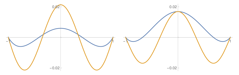
Figure 1: Graphs of $f_{s}$ (blue) and $f_{d}$ (orange) for “the optimal” approximant from [1] (left) and for the optimal approximant constructed in this paper (right). In all cases $a=1/\sqrt{3}$. It is clearly seen that the one on the right has a smaller error on $\angle$.

3 Main result

To prove that the optimal approximant $f_{s}$ can not equioscillate, let us start with the following important observation.

Lemma 3.1

For every $u\in[0,1)$ and $\alpha,\beta>0$ functions $f_{s}(u,\cdot)$, $f_{d}(u,\cdot,\beta)$, and $f_{d}(u,\alpha,\cdot)$ are strictly increasing.

Proof 1

The result of the lemma follows directly from the observations

$$\frac{\partial f_{s}}{\partial\alpha}(u,\alpha) =\left(1-a^{2}\right)\left(1-u^{2}\right)\left(1+u^{2}+2\alpha\left(1-u^{2}\right)\right),$$

$$\frac{\partial f_{d}}{\partial\alpha}(u,\alpha,\beta) =\frac{1}{2}\sqrt{1-2a^{2}}\beta\left(1-u^{4}\right)\left(1-u^{2}\right)^{2}+2\alpha\left(1-2a^{2}\right)\left(1-u^{4}\right)^{2}$$

$$+4a^{2}\alpha u^{2}\left(1-u^{2}\right)^{2}+\frac{1}{2}\left(1-2a^{2}\right)\left(1-u^{8}\right)+u^{2}\left(1-u^{4}\right),$$

$$\frac{\partial f_{d}}{\partial\beta}(u,\alpha,\beta) =\frac{1}{8}\left(1-u^{2}\right)^{2}\left(\beta\left(1-u^{2}\right)^{2}+\sqrt{1-2a^{2}}\left(1+u^{2}\right)^{2}+4\sqrt{1-2a^{2}}\alpha\left(1-u^{4}\right)\right).$$

Quite clearly this lemma implies that $f_{s,d}(\cdot,\alpha^{*},\beta^{*})$ must equioscillate. Moreover, we will show that $f_{d}(\cdot,\alpha^{*},\beta^{*})$ equioscillates and $f_{s}$ does not, which contradict the results in [1]. Let us prove a particular relation between $f_{d}$ and $f_{s}$ first.

Lemma 3.2

Let $\alpha\in\left[\tfrac{1}{2},\tfrac{1}{2-2a^{2}}\right]$ and let $f_{d}(0,\alpha,\beta)\leq f_{s}(0,\alpha)$. Then $f_{d}(u,\alpha,\beta)<f_{s}(u,\alpha)$ for all $u\in(0,1)$.

Proof 2

Let us assume first that $f_{d}(0,\alpha,\beta)=f_{s}(0,\alpha)$. Then

$$\beta=\beta(\alpha)=2(1+2\alpha)\sqrt{1-a^{2}}-(1+4\alpha)\sqrt{1-2a^{2}}.$$

If we define $\alpha(t)=\frac{a^{2}}{2\left(1-a^{2}\right)}t+\frac{1}{2}$, then for $t\in[0,1]$ we have $\alpha(t)\in\left[\tfrac{1}{2},\tfrac{1}{2-2a^{2}}\right]$ and it is eqnough to show that $h(t)=f_{s}(u,\alpha(t))-f_{d}(u,\alpha(t),\beta(\alpha(t)))>0$ for all $t\in[0,1]$ and $u\in(0,1)$. But this follows directly from

$$h(t) =u^{2}\left(1-u^{2}\right)\left(2\left(1-\sqrt{1-2a^{2}}\sqrt{1-a^{2}}-\frac{3a^{2}}{2}\right)\left(1-u^{2}\right)\left(2-u^{2}\right)+a^{2}\right)(1-t)$$

$$+\frac{u^{2}\left(1-u^{2}\right)^{2}}{1-a^{2}}\left(\left(1-\sqrt{1-2a^{2}}\sqrt{1-a^{2}}-\frac{3a^{2}}{2}\right)\left(4-2u^{2}-a^{2}u^{2}\right)+\frac{a^{4}u^{2}}{2}\right)t(1-t)$$

$$+\frac{u^{2}\left(1-u^{2}\right)^{2}}{4\left(1-a^{2}\right)^{2}}\left(\left(1-\sqrt{1-2a^{2}}\sqrt{1-a^{2}}-\frac{3a^{2}}{2}-\frac{a^{4}}{8}\right)\left(8-4a^{2}\right)\left(2-a^{2}-u^{2}\right)+\frac{1}{2}a^{6}\left(a^{2}+3u^{2}\right)\right)t^{2}.$$

If $f_{d}(0,\alpha,\beta)<f_{s}(0,\alpha)=f_{d}(0,\alpha,\beta(\alpha))$ then by Lemma 3.1 $\beta<\beta(\alpha)$ and we conclude that $f_{d}(u,\alpha,\beta)<f_{d}(u,\alpha,\beta(\alpha))\leq f_{s}(u,\alpha)$ for all $u\in(0,1)$.

Note that

$$f_{s}\left(u,\frac{1}{2}\right)=-a^{2}(1-u^{2})\leq 0\quad\text{and}\quad f_{s}\left(u,\frac{1}{2(1-a^{2})}\right)=\frac{a^{4}(1-u^{2})^{2}}{4(1-a^{2})}\geq 0,$$ (4)

thus the parameter $\alpha_{e}$ for which $f_{s}(\cdot,\alpha)$ equioscillates must be on the interval $I=\left[\tfrac{1}{2},\tfrac{1}{2(1-a^{2})}\right]$. But unfortunately, it may happen that $\alpha^{*}\not\in I$. Thus we define an enlarged interval $I_{0}=\left[\tfrac{1}{2},\tfrac{3}{2}\right]\supset I$ which will be used in further analysis.

Corollary 3.3

If $f_{s}(\cdot,\alpha_{e})$ equioscillates, then for every $\beta>0$

$$\max_{u\in[-1,1]}\left|f_{d}(u,\alpha_{e},\beta)\right|>\max_{u\in[-1,1]}\left|f_{s}(u,\alpha_{e})\right|.$$

Proof 3

Let us suppose that

$$\max_{u\in[-1,1]}\left|f_{d}(u,\alpha_{e},\beta)\right|\leq\max_{u\in[-1,1]}\left|f_{s}(u,\alpha_{e})\right|.$$

Since $\max_{u\in[-1,1]}\left|f_{s}(u,\alpha_{e})\right|=f_{s}(0,\alpha_{e})$, we have $f_{d}(0,\alpha_{e},\beta)\leq f_{s}(0,\alpha_{e})$ and by Lemma 3.2

$$f_{d}(u,\alpha_{e},\beta)<f_{s}(u,\alpha_{e}),\quad u\in(0,1).$$

Consequently $\min_{u\in[-1,1]}f_{d}(u,\alpha_{e},\beta)<\min_{u\in[-1,1]}f_{s}(u,\alpha_{e})$ which is a contradiction.

Lemma 3.4

If $(\alpha^{*},\beta^{*})$ is an optimal pair of parameters then

$$\min_{u\in[-1,1]}f_{s,d}(u,\alpha^{*},\beta^{*})=\min_{u\in[-1,1]}f_{d}(u,\alpha^{*},\beta^{*})\quad\text{and}\quad\max_{u\in[-1,1]}f_{s,d}(u,\alpha^{*},\beta^{*})=\max_{u\in[-1,1]}f_{d}(u,\alpha^{*},\beta^{*}).$$

Proof 4

Since minimum and maximum of $f_{s,d}$ is attained either by $f_{s}$ or $f_{d}$, four possibilities have to be considered.
If

$$\min_{u\in[-1,1]}f_{s}(u,\alpha^{*})<\min_{u\in[-1,1]}f_{d}(u,\alpha^{*},\beta^{*})\quad{\rm and}\quad\max_{u\in[-1,1]}f_{d}(u,\alpha^{*},\beta^{*})>\max_{u\in[-1,1]}f_{s}(u,\alpha^{*})$$

or

$$\min_{u\in[-1,1]}f_{d}(u,\alpha^{*},\beta^{*})<\min_{u\in[-1,1]}f_{s}(u,\alpha^{*})\quad{\rm and}\quad\max_{u\in[-1,1]}f_{s}(u,\alpha^{*})>\max_{u\in[-1,1]}f_{d}(u,\alpha^{*},\beta^{*})$$

then since $f_{s}$ does not depend on $\beta$ and $f_{d}$ is an increasing function of $\beta$, we can find $\beta^{**}<\beta^{*}$ or $\beta^{**}>\beta^{*}$ that $(\alpha^{*},\beta^{**})$ implies a better approximant, respectively.
If $\max_{u\in[-1,1]}f_{s}(u,\alpha^{*})>\max_{u\in[-1,1]}f_{d}(u,\alpha^{*},\beta^{*})$ then

$$\max_{u\in[-1,1]}f_{s}(u,\alpha^{*})=f_{s}(0,\alpha^{*})>\max_{u\in[-1,1]}f_{d}(u,\alpha^{*},\beta^{*})$$

and the case $\min_{u\in[-1,1]}f_{s}(u,\alpha^{*})<\min_{u\in[-1,1]}f_{d}(u,\alpha^{*},\beta^{*})$ is not possible due to the Lemma 3.2. This confirms the result of the lemma.

The previous lemma reveals that we are looking for an optimal error $f_{d}$, i.e., an equioscillating $f_{d}$. This is still a two-dimensional optimization problem. But we shall prove that for the optimal pair of parameters $\alpha^{*}$ and $\beta^{*}$ we must have $f_{s}(0,\alpha^{*})=f_{d}(0,\alpha^{*},\beta^{*})$ which leads to one-dimensional optimization. Namely, the quadratic function $\beta\mapsto f_{d}(0,\alpha,\beta)-f_{s}(0,\alpha)$ has positive leading coefficient and negative constant term, therefore it possesses the unique positive zero

$$\beta=\beta_{0}(\alpha)=2(1+2\alpha)\sqrt{1-a^{2}}-(1+4\alpha)\sqrt{1-2a^{2}}.$$

This leads to the following observation.

Lemma 3.5

If $f_{s}(0,\alpha)=f_{d}(0,\alpha,\beta)=0$, then $f_{s}(u,\alpha)\leq 0$ and $f_{d}(u,\alpha,\beta)\leq 0$ for all $u\in[-1,1]$.

Proof 5

The solution of the system $f_{s}(0,\alpha)=0$ and $f_{d}(0,\alpha,\beta)=0$ is

$$\alpha=\frac{1}{\sqrt{1-a^{2}}}-\frac{1}{2}\quad{\rm and}\quad\beta=\beta_{0}\left(\frac{1}{\sqrt{1-a^{2}}}-\frac{1}{2}\right)=4+\sqrt{1-2a^{2}}\left(1-\frac{4}{\sqrt{1-a^{2}}}\right).$$

Consequently

$$f_{s}(u,\alpha)=-\left(1-\sqrt{1-a^{2}}\right)^{2}u^{2}(1-u^{2})\leq 0$$

and

$$f_{d}(u,\alpha,\beta)=-\frac{2u^{2}\left(1-u^{2}\right)}{1-a^{2}}\left(2\left(1-\sqrt{1-a^{2}}-\frac{a^{2}}{2}\right)u^{2}\left(u^{2}\left(1-a^{2}\right)+a^{2}\left(1-u^{2}\right)\right)\right.\\ +\left.\left(1-u^{2}\right)^{2}\left(\sqrt{1-2a^{2}}-\sqrt{1-a^{2}}\right)^{2}+\left(1-\sqrt{1-2a^{2}}-a^{2}\right)u^{2}\left(1-u^{2}\right)\left(1-a^{2}\right)\right)\leq 0$$

for $u\in[-1,1]$.

If the assumption $f_{s}(0,\alpha)=f_{d}(0,\alpha,\beta)=0$ is extended to $f_{s}(0,\alpha)=f_{d}(0,\alpha,\beta)\geq 0$, the following result can be confirmed.

Lemma 3.6

Let $f_{d}(0,\alpha,\beta)=f_{s}(0,\alpha)\geq 0$. Then

$$\frac{df_{d}}{d\alpha}(0,\alpha,\beta_{0}(\alpha))\geq\frac{df_{d}}{d\alpha}(u,\alpha,\beta_{0}(\alpha))$$

for all $u\in[-1,1]$.

Proof 6

Recall that $\alpha\geq\frac{1}{2}$ and observe that

$$\frac{df_{d}}{d\alpha}(0,\alpha,\beta_{0}(\alpha))-\frac{df_{d}}{d\alpha}(u,\alpha,\beta_{0}(\alpha))=2u^{2}\left(k(\alpha-\tfrac{1}{2})+n\right),$$

where

$$k= \left(\sqrt{1-2a^{2}}-\sqrt{1-a^{2}}\right)^{2}\left(1-u^{2}\right)\left(2\left(1-u^{2}\right)^{2}+u^{2}+u^{4}\right)$$

$$+2\left(\sqrt{1-2a^{2}}\sqrt{1-a^{2}}\right)u^{2}\left(1-u^{4}\right)+u^{6}\left(1-a^{2}\right)+a^{2}u^{2}\left(1-u^{2}\right)\left(3-u^{2}\right)\geq 0,$$

$$n= 2\left(\sqrt{1-2a^{2}}-\sqrt{1-a^{2}}\right)^{2}\left(2-5u^{2}+5u^{4}-\frac{3u^{6}}{2}\right)$$

$$+\sqrt{1-2a^{2}}\sqrt{1-a^{2}}u^{2}+a^{2}\left(u^{2}-u^{4}+\frac{u^{6}}{2}\right)\geq 0.$$

Corollary 3.7

If $f_{s}(0,\alpha)=f_{d}(0,\alpha,\beta)\geq 0$ then $\max f_{s}(\cdot,\alpha)=\max f_{d}(\cdot,\alpha,\beta)=f_{s}(0,\alpha)$.

Proof 7

Since

$$f_{s}\left(u,\frac{1}{\sqrt{1-a^{2}}}-\frac{1}{2}\right)=-\left(1-\sqrt{1-a^{2}}\right)^{2}u^{2}\left(1-u^{2}\right)\leq 0$$

the inequality $f_{s}(0,\alpha)\geq 0$ implies $\alpha\geq\alpha_{0}=\frac{1}{\sqrt{1-a^{2}}}-\frac{1}{2}$. Since $\alpha_{0}\in[\frac{1}{2},\frac{1}{2-2a^{2}}]$, Lemma 3.2 implies $f_{d}(u,\alpha_{0},\beta_{0}(\alpha_{0}))\leq 0$ for all $u\in[-1,1]$. The result now follows from Lemma 3.6.

Lemma 3.8

Let $f_{d}(0,\alpha,\beta)>f_{s}(0,\alpha)\geq 0$. Let $\alpha^{\prime}$ and $\beta^{\prime}$ be such that $f_{s}(0,\alpha^{\prime})=f_{d}(0,\alpha,\beta)=f_{s}(0,\alpha^{\prime},\beta^{\prime})$. Then $f_{d}(u,\alpha,\beta)\leq f_{d}(u,\alpha^{\prime},\beta^{\prime})\leq f_{d}(0,\alpha,\beta)$ for all $u\in[-1,1]$.

Proof 8

For every $\mu\in[f_{s}(0,\alpha),f_{d}(0,\alpha,\beta)]$ let $\alpha(\mu)$ be the only positive solution of $f_{s}(0,\alpha(\mu))=\mu$, let $\beta(\mu)$ be the only positive solution of $f_{d}(0,\alpha(\mu),\beta(\mu))=\mu$, and $\beta_{\alpha}(\mu)$ be the only positive solution of $f_{d}(0,\alpha,\beta(\mu))=\mu$. Then

$$\alpha(\mu) =\frac{2\sqrt{1+\mu}\sqrt{1-a^{2}}-1+a^{2}}{2\left(1-a^{2}\right)},$$

$$\beta(\mu) =\frac{\left(\sqrt{1-2a^{2}}+4\sqrt{1+\mu}\right)\left(1-a^{2}\right)-4\sqrt{1+\mu}\sqrt{1-2a^{2}}\sqrt{1-a^{2}}}{1-a^{2}},$$

$$\beta_{\alpha}(\mu) =4\sqrt{1+\mu}-(1+4\alpha)\sqrt{1-2a^{2}}.$$

For $\mu_{0}=f_{s}(0,\alpha)$, we have $\alpha=\alpha(\mu_{0})$, hence $f_{d}(u,\alpha,\beta_{\alpha}(\mu_{0}))=f_{d}(u,\alpha(\mu_{0}),\beta(\mu_{0}))$ for all $u\in[-1,1]$. So it is enough to prove that $\tfrac{\partial f_{d}}{\partial\mu}(u,\alpha,\beta(\mu))\leq\tfrac{\partial f_{d}}{\partial\mu}(u,\alpha(\mu),\beta(\mu))$. Since

$$\tfrac{\partial f_{d}}{\partial\mu}(u,\alpha(\mu),\beta(\mu))-\tfrac{\partial f_{d}}{\partial\mu}(u,\alpha,\beta(\mu))=\frac{u^{2}\left(1-u^{2}\right)\left(A_{1}\left(\frac{3}{2}-\alpha\right)+A_{2}\left(\sqrt{1+\mu}-1\right)+A_{3}\right)}{\left(1-a^{2}\right)\sqrt{1+\mu}},$$

where

$$A_{1} =2\sqrt{1-2a^{2}}\left(1-a^{2}\right)\left(1-u^{2}\right)^{2}\geq 0,$$

$$A_{2} =2\left(1-u^{2}\right)\left(2\left(1-u^{2}\right)\sqrt{1-2a^{2}}\sqrt{1-a^{2}}+2u^{2}\left(1-2a^{2}\right)+a^{2}\right)\geq 0,$$

$$A_{3} =2\sqrt{1-2a^{2}}\sqrt{1-a^{2}}2\left(1-u^{2}\right)^{2}\left(1-\sqrt{1-a^{2}}\right)$$

$$+2\left(\sqrt{1-a^{2}}\left(u^{4}\left(1-2a^{2}\right)+a^{2}u^{2}\right)+\left(1-u^{2}\right)\left(\left(1-2a^{2}\right)2u^{2}+a^{2}\right)\right)\geq 0,$$

the lemma follows.

It is clear now that parameters $(\alpha^{*},\beta^{*})$ are such that $|f|$ restricted on $\angle$ has the smallest possible minimum. We will now prove that $f(\cdot,\cdot,\alpha^{*},\beta^{*})$ has local extrema only on the diagonals and on the sides of the square $[-1,1]^{2}$.

The function $f(\cdot,\cdot,\alpha,\beta)$ is a symmetric polynomial. Let us reparameterize it by $e_{1}=u^{2}+v^{2}$ and $e_{2}=u^{2}v^{2}$. The map $(u,v)\mapsto(u^{2}+v^{2},u^{2}v^{2})=(e_{1},e_{2})$ is a bijection between $T=\{(u,v)\in\mathbb{R}^{2};0<u<1,0<v<u\}$ and $S=\{(e_{1},e_{2})\in\mathbb{R}^{2};0<e_{1}<2,e_{1}-1<e_{2}<\tfrac{1}{4}e_{1}^{2},e_{2}>0\}$. If we write $h(e_{1},e_{2},\alpha)=f(u,v,\alpha,\beta_{0}(\alpha))$, the map $f(\cdot,\cdot,\alpha,\beta_{0}(\alpha))$ has local extrema on $T$ if and only if $h(\cdot,\cdot,\alpha)$ has local extrema on $S$. But $h(\cdot,\cdot,\alpha)$ as a function on $\mathbb{R}^{2}$ has only one local extreme point $(x,y)$, namely

$$x =\frac{4(1+2\alpha)\left(\alpha(1-2\alpha)\left(2-4\alpha+a^{2}(3+2\alpha)\right)+\left(1+7\alpha+8\alpha^{2}-20\alpha^{3}\right)\left(\sqrt{1-2a^{2}}-\sqrt{1-a^{2}}\right)^{2}\right)}{(1-2\alpha)^{2}(6\alpha+1)\left((14\alpha+5)a^{2}+4\left(\sqrt{1-2a^{2}}\sqrt{1-a^{2}}-1\right)(2\alpha+1)\right)},$$

$$y =\frac{(1+2\alpha)^{2}\left(a^{2}\left(1-4\alpha^{2}\right)+2\left(5+2\alpha-8\alpha^{2}\right)\left(\sqrt{1-2a^{2}}-\sqrt{1-a^{2}}\right)^{2}\right)}{(1-2\alpha)^{2}(1+6\alpha)\left(a^{2}(2\alpha-1)-2(1+2\alpha)\left(\sqrt{1-2a^{2}}-\sqrt{1-a^{2}}\right)^{2}\right)}.$$

We shall see that for $\alpha=\alpha^{*}$ we have $y>1$, which implies that $h(\cdot,\cdot,\alpha^{*})$ has no local extrema on $T$.

Let us first prove that $\tfrac{1-\tfrac{1}{5}a^{4}}{2(1-a^{2})}=:\alpha_{l}<\alpha^{*}<\tfrac{1+\tfrac{1}{5}a^{4}}{2(1-a^{2})}=:\alpha_{r}$. Since $f_{s}(0,\alpha_{l})=\frac{a^{4}\left(5+10a^{2}+a^{4}\right)}{100\left(1-a^{2}\right)}\geq 0$, the functions $f_{s}(\cdot,\cdot,\alpha)$ and $f_{d}(\cdot,\cdot,\alpha,\beta_{0}(\alpha))$ have the maximum at $u=0$ for all $\alpha\in[\alpha_{l},\alpha_{r}]$. We can write

$$f_{d}\left(\frac{3}{4},\alpha_{l},\beta_{0}(\alpha_{l})\right)+f_{d}\left(0,\alpha_{l},\beta_{0}(\alpha_{l})\right)=-\frac{\eta}{6553600(1-a^{2})^{2}(\zeta\sqrt{1-a^{2}}\sqrt{1-2a^{2}}+\xi)}\leq 0,$$

where

$$\eta=a^{4}\sum_{i=0}^{8}\eta_{i}a^{2i}(1-2a^{2})^{8-i},\quad\zeta=\sum_{i=0}^{4}\zeta_{i}a^{2i}(1-2a^{2})^{4-i},\quad\xi=\sum_{i=0}^{5}\xi_{i}a^{2i}(1-2a^{2})^{5-i},$$

such that $\eta_{i},\zeta_{i},\xi_{i}>0$ for all $i$. Hence the minimum of $\left|f_{d}\left(\cdot,\cdot,\alpha_{l},\beta_{0}(\alpha_{l})\right)\right|$ is larger then the maximum, therefore $\alpha^{*}>\alpha_{l}$. On the other hand, we can write

$$f_{d}\left(u,\alpha_{r},\beta_{0}(\alpha_{r})\right)+f_{d}\left(0,\alpha_{r},\beta_{0}(\alpha_{r})\right)=\frac{\zeta\sqrt{1-a^{2}}\sqrt{1-2a^{2}}+\xi}{100(1-a^{2})^{2}},$$

where $\zeta=4\left(10-5a^{2}+a^{4}\right)u^{2}\left(1-u^{2}\right)^{2}\left(5\left(2-a^{2}-u^{2}\right)+a^{4}\left(1-u^{2}\right)\right)\geq 0$. Since $\sqrt{1-a^{2}}\sqrt{1-2a^{2}}\geq 1-\tfrac{3}{2}a^{2}-a^{4}$ for all $a\in[0,\tfrac{\sqrt{2}}{2}]$, we have

$$f_{d}\left(u,\alpha_{r},\beta_{0}(\alpha_{r})\right)+f_{d}\left(0,\alpha_{r},\beta_{0}(\alpha_{r})\right)=\frac{\zeta\sqrt{1-a^{2}}\sqrt{1-2a^{2}}+\xi}{100(1-a^{2})^{2}}\geq\frac{\zeta(1-\tfrac{3}{2}a^{2}-a^{4})+\xi}{100(1-a^{2})^{2}}.$$

Since we can write

$$\zeta(1-\tfrac{3}{2}a^{2}-a^{4})+\xi=\sum_{i=0}^{4}\left(\sum_{j=0}^{9-i}k_{i,j}u^{2j}(1-u^{2})^{9-i-j}\right)a^{12-2i}(1-2a^{2})^{i},$$

where all coefficients $k_{i,j}>0$, we have $f_{d}\left(u,\alpha_{r},\beta_{0}(\alpha_{r})\right)+f_{d}\left(0,\alpha_{r},\beta_{0}(\alpha_{r})\right)\geq 0$ for all $u\in[-1,1]$. Hence the maximum of $\left|f_{d}\left(\cdot,\cdot,\alpha_{r},\beta_{0}(\alpha_{r})\right)\right|$ is larger then the minimum, therefore $\alpha^{*}<\alpha_{r}$.

Let us write $\alpha=(1-t)\alpha_{l}+t\alpha_{r}$ and prove that $y>1$ for all $t\in[0,1]$, in particular, $y>1$ for $\alpha=\alpha^{*}$. Let us write $y=\tfrac{y_{n}}{y_{d}}$. Let us first show that $y_{d}<0$. We can write

$$-\frac{5(1-2a^{2})}{(1-2\alpha)^{2}(1+6\alpha)}y_{d}=\xi+\zeta\sqrt{1-2a^{2}}\sqrt{1-a^{2}},$$

where $\xi=40(1-2a^{2})^{3}+160a^{2}(1-2a^{2})^{2}+181a^{4}(1-2a^{2})+49a^{6}+8a^{4}(1-2a^{2})t+2a^{6}t$ and $\zeta=4(a^{4}(1-2t)-5(2-a^{2})$. Since $\xi>0$ for all $t\in[0,1]$ it is enough to show that $\xi^{2}-\left(\zeta\sqrt{1-2a^{2}}\sqrt{1-a^{2}}\right)^{2}>0$. This follows from the equality

$$\xi^{2}-\left(\zeta\sqrt{1-2a^{2}}\sqrt{1-a^{2}}\right)^{2}=17a^{12}(1-2t)^{2}+480a^{6}(1-a^{2})(1-t)+320ta^{6}+12a^{10}t+\\ 25a^{8}(1-2a^{2})t+105a^{8}(1-2a^{2})(1-t)+232a^{10}(1-t)+32ta^{10}(1-t)>0.$$

Hence to prove $y>1$, we have to show that $y_{d}-y_{n}>0$. We can write

$$y_{d}-y_{n} =\xi\sqrt{1-a^{2}}\sqrt{1-2a^{2}}-\zeta=\frac{(\xi\sqrt{1-a^{2}}\sqrt{1-2a^{2}}+k)^{2}-(\zeta+k)^{2}}{\xi\sqrt{1-a^{2}}\sqrt{1-2a^{2}}+\zeta+2k}$$

$$\geq\frac{2k\xi\sqrt{1-a^{2}}\sqrt{1-2a^{2}}+\xi^{2}(1-a^{2})(1-2a^{2})-\zeta^{2}-2k\zeta}{\xi\sqrt{1-a^{2}}\sqrt{1-2a^{2}}+\zeta+2k}$$

$$\geq\frac{2k\xi(1-\frac{3}{2}a^{2}-\frac{1}{8}a^{4}-\frac{7}{4}a^{6})+\xi^{2}(1-a^{2})(1-2a^{2})-\zeta^{2}-2k\zeta}{\xi\sqrt{1-a^{2}}\sqrt{1-2a^{2}}+\zeta+2k},$$

where $k=\tfrac{103901}{256}$ and

$$\xi =\frac{1}{625(1-a^{2})^{4}}\left(\sum_{i=0}^{15}\sum_{j=0}^{3}\xi_{i,j}a^{2i}(1-2a^{2})^{15-i}t^{j}(1-t)+\sum_{i=0}^{15}\xi_{i,4}a^{2i}(1-2a^{2})^{15-i}t^{4}\right),$$

$$\zeta =\frac{1}{625(1-a^{2})^{4}}\left(\frac{1}{256}\left(\sum_{i=0}^{15}\sum_{j=0}^{3}\zeta_{i,j}a^{2i}(1-2a^{2})^{15-i}t^{j}(1-t)+\sum_{i=0}^{15}\zeta_{i,4}a^{2i}(1-2a^{2})^{15-i}t^{4}\right)+2k\right),$$

$$2k\xi (1-\frac{3}{2}a^{2}-\frac{1}{8}a^{4}-\frac{7}{4}a^{6})+\xi^{2}(1-a^{2})(1-2a^{2})-\zeta^{2}-2k\zeta$$

$$=\sum_{i=0}^{15}\sum_{j=0}^{8}\eta_{i,j}a^{2i+6}(1-2a^{2})^{15-i}t^{j}(1-t)+\sum_{i=0}^{15}\eta_{i,9}a^{2i+6}(1-2a^{2})^{15-i}t^{9},$$

and all coefficients $\xi_{i,j}$, $\zeta_{i,j}$ and $\eta_{i,j}$ are positive. Hence $y>1$ and the maximum and minimum of $f(\cdot,\alpha^{*},\beta^{*})$ are on the diagonals or on the sides of the square $[-1,1]^{2}$. Thus we have proved the following crucial theorem.

Theorem 3.9

The maximum and the minimum of $f(\cdot,\cdot,\alpha,\beta)$ are on the set $\angle$.

It is quite clear now how to find the best approximant. The procedure is identical for the simplified radial error and for the radial error by replacing $f$ by $g$ so we consider only the first one.

• Solve the equation $f_{d}(0,\alpha,\beta)=f_{s}(0,\alpha)$ on $\beta$ to get the admissible $\beta_{0}(\alpha):=\beta(\alpha)$.

• Solve the system of nonlinear equations

  $$\frac{\partial f_{d}}{\partial u}(u,\alpha,\beta_{0}(\alpha)) =0,$$

  $$f_{d}(0,\alpha,\beta_{0}(\alpha))+f_{d}(u,\alpha,\beta_{0}(\alpha)) =0$$

  on $u$ and $\alpha$ to get the admissible solution $u_{0}$ and $\alpha_{0}$.

• Return the best approximant $\boldsymbol{p}$ constructed by $\alpha_{0}$ and $\beta_{0}(\alpha_{0})$.

Note that the above algorithm must be performed numerically since the equation in b) can not be solved in a closed form in general. The Newton-Raphson method might be used or any other appropriate algorithm for solving the system of nonlinear equations.

4 Optimal $G^{1}$ approximation

A natural question arises whether the optimal approximant of the spherical square constructed in the previous section can be used as a $G^{1}$ tensor product quadratic Bézier spline approximant of the unit sphere. In this case, either two or six patches can be put together. We shall focus only on the spline of six patches since even in this case the obtained $G^{1}$ surface is not a good approximation of the sphere.
If six patches are put together we have $a=\tfrac{\sqrt{3}}{3}$. The $G^{1}$ condition implies that the tangent plane of each of the three patches meeting at the common corner point must coincide with the tangent plane of a sphere. Hence $\tfrac{\partial\boldsymbol{p}}{\partial u}(-1,-1)\times\tfrac{\partial\boldsymbol{p}}{\partial v}(-1,-1)=[\tfrac{2}{3}(1-2\alpha)\alpha,\tfrac{2}{3}(1-2\alpha)\alpha,\tfrac{4}{3}(1-\alpha)\alpha]^{T}$ must be parallel to the unit normal of $\boldsymbol{p}$ at $(-1,-1)$, i.e., parallel to $[-\tfrac{\sqrt{3}}{3},-\tfrac{\sqrt{3}}{3},\tfrac{\sqrt{3}}{3}]^{T}$. This implies $\alpha_{G}=\tfrac{3}{4}$. For every $v\in[0,1]$ the tangent plane at points $\boldsymbol{p}(1,v)$ and $R\boldsymbol{p}(0,v)$, where $R$ is the rotation matrix around $y$-axis for the angle $\tfrac{\pi}{2}$, must coincide. Due to the symmetry, the normal vector of the tangent plane must lie in the plane defined by $\boldsymbol{b}_{20}$, $\boldsymbol{b}_{22}$, and the origin. Therefore $\tfrac{\partial\boldsymbol{p}}{\partial u}(-1,v)\times\tfrac{\partial\boldsymbol{p}}{\partial v}(-1,v)$ must be perpendicular to $\boldsymbol{p}(1,-1)\times\boldsymbol{p}(1,1)$ which implies $\beta_{G}=\tfrac{7\sqrt{3}}{6}$. So the $G^{1}$ spline approximant is unique and its radial error is $\left|g(0,0,\alpha_{G},\beta_{G})\right|=\tfrac{5\sqrt{3}-8}{8}\approx 0.0825$ which is much bigger than the radial error of the corresponding $G^{0}$ spline of six optimal approximants constructed in the previous section (see Figure 4 and Figure 5).

5 Rectangular case

Another interesting issue is the optimal approximation of a spherical rectangle. Recall that in the case of the approximation of a spherical square, the minimum of the simplified radial error was never attained at the boundary of a patch. The situation is quite different in the case of the approximation of a spherical rectangle. The explanation will be supported by numerical evidence but no formal proof will be provided.
Let the projection of the vertices of a spherical rectangle along the vector $[0,0,1]^{T}$ be vertices of a planar rectangle with its larger edge $2a$ fixed and let $2b<2a$ be it shorter edge. Similarly, as in the case of a spherical square (1), we define a tensor product quadratic Bézier patch $\boldsymbol{p}_{r}$ as

$$\boldsymbol{p}_{r}(u,v,\alpha_{1},\alpha_{2},\beta)=\sum_{i=0}^{2}\sum_{j=0}^{2}B_{i}^{2}(u)B_{j}^{2}(v)\boldsymbol{c}_{ij},\quad u,v\in[-1,1],$$

where, analogously as in (3),

$$\boldsymbol{c}_{00}=(-a,-b,\sqrt{1-a^{2}-b^{2}}),\quad \boldsymbol{c}_{10}=\alpha_{1}(\boldsymbol{c}_{00}+\boldsymbol{c}_{20}),\quad \boldsymbol{c}_{20}=(a,-b,\sqrt{1-a^{2}-b^{2}}),\quad$$

$$\boldsymbol{c}_{01}=\alpha_{2}(\boldsymbol{c}_{00}+\boldsymbol{c}_{02}),\quad \boldsymbol{c}_{11}=\beta\,(0,0,1),\quad \boldsymbol{c}_{21}=\alpha_{2}(\boldsymbol{c}_{20}+\boldsymbol{c}_{22}),\quad$$ (5)

$$\boldsymbol{c}_{02}=(-a,b,\sqrt{1-a^{2}-b^{2}}),\quad \boldsymbol{c}_{12}=\alpha_{1}(\boldsymbol{c}_{02}+\boldsymbol{c}_{22}),\quad \boldsymbol{c}_{22}=(a,b,\sqrt{1-a^{2}-b^{2}}),$$

with some $\alpha_{1},\alpha_{2},\beta>0$. As in (2), we define $f_{r}(\cdot,\cdot,\alpha_{1},\alpha_{2},\beta)=\left\|\boldsymbol{p}_{r}(\cdot,\cdot,\alpha_{1},\alpha_{2},\beta)\right\|^{2}-1.$ We have seen in the analysis of the square case that the global minimum of $f$ can not appear on the boundary of the square $[-1,1]^{2}$. We shall see in the following that this can actually happen in the rectangular case for some particular ratio of sides $a$ and $b$. Once the global minimum is on the boundary, numerical examples confirm that several optimal approximants of the spherical rectangle might exist. This indicates that the rectangular case is a much more challenging problem.
Let us now try to find the condition on $b$, which implies that the global minimum and maximum of $f$ are on the boundary. If this is the case, we can assume that the restriction of $f_{r}$ on $(u,-1)$, $u\in[-1,1]$, equioscillate. This implies the parameter $\alpha_{1}$ and the point $u_{0}\in(-1,0)$ such that $\tfrac{\partial f_{r}}{\partial u}(u_{0},-1,\alpha_{1},\alpha_{2},\beta)=0$ and $f_{r}(u_{0},-1,\alpha_{1},\alpha_{2},\beta)$ is the global minimum of $f_{r}$ for any $\alpha_{2}$ and $\beta$. A necessary condition for $f_{r}(u_{0},-1,\alpha_{1},\alpha_{2},\beta)$ being the global minimum is $\tfrac{\partial f_{r}}{\partial v}(u_{0},-1,\alpha_{1},\alpha_{2},\beta)\geq 0$. Suppose that the triple $(b_{a},\alpha_{a},\beta_{a})$ is the solution of the system of nonlinear equations

$$\tfrac{\partial f_{r}}{\partial v}(u_{0},-1,\alpha_{1},\alpha_{2},\beta)=0,$$

$$f_{r}(0,-1,\alpha_{1},\alpha_{2},\beta)=f_{r}(0,0,\alpha_{1},\alpha_{2},\beta),$$

$$f(0,-1,\alpha_{1},\alpha_{2},\beta)=f(-1,0,\alpha_{1},\alpha_{2},\beta),$$

with respect to $b$, $\alpha_{2}$ and $\beta$. For every $b=b_{a}$, the candidate for the best approximant of the spherical rectangle related to $a$ and $b_{a}$ is determined by the parameters $(\alpha_{1},\alpha_{a},\beta_{a})$. If $b<b_{a}$ all pairs of parameters $(\alpha_{2},\beta)$ satisfying the inequalities

$$\tfrac{\partial f}{\partial v}(u_{0},-1,\alpha_{1},\alpha_{2},\beta) \geq 0,$$

$$f(0,-1,\alpha_{1},\alpha_{2},\beta) \geq f(0,0,\alpha_{1},\alpha_{2},\beta),$$ (6)

$$f(0,-1,\alpha_{1},\alpha_{2},\beta) \geq f(-1,0,\alpha_{1},\alpha_{2},\beta),$$

might induce the best approximant. Thus, in this case, we might have an uncountable number of optimal polynomial approximants of the spherical rectangle. Indeed, let $\boldsymbol{v}_{i}=(\alpha_{2,i},\beta_{i})$, $i=1,2,3$, be the intersections of two pairs of curves in (6) which are implicitly defined by taking equalities instead of inequalities. Numerical computations indicate that all pairs $(\alpha_{2},\beta)$ from the triangle defined by $\boldsymbol{v}_{i}$, $i=1,2,3$, imply an optimal approximant. Moreover, numerical computations also indicate that several optimal approximant might exist if a pair $(a,b)$ is taken from the grey region in Figure 2. On Figure 3, radial errors of three optimal approximants of the spherical rectangle with $a=0.75$ and $b=0.2$ are shown.

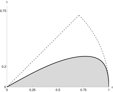
Figure 2: The domain (light grey) in $[0,1]^{2}$ for which pairs $(a,b)$ might imply several optimal approximants of the spherical rectangle. The grey dashed curve is the graph of the function $\min\{a,\sqrt{1-a^{2}}\}$ and together with the $a$-axis determine the admissible domain of pairs $(a,b).$

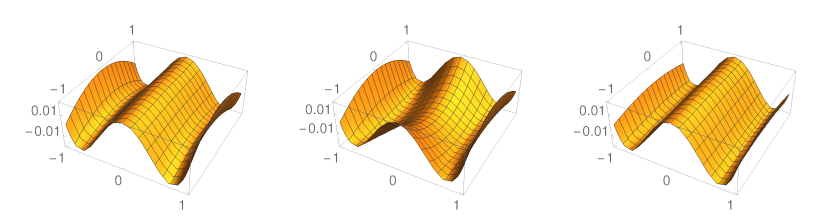
Figure 3: Graphs of $f$ for three optimal approximants of the spherical rectangle given by parameters $a=0.75$ and $b=0.2$. Here $\alpha_{1}=1.0277$ and the left graph corresponds to the pair $(\alpha_{2},\beta)=(0.5313,1.4456)$, the middle one to $(\alpha_{2},\beta)=(0.5313,1.3881)$, and the right one to $(\alpha_{2},\beta)=(0.5239,1.4550)$.

6 Numerical examples

Some numerical examples will be presented in this section, confirming proven theoretical results. As the first example, let us consider the optimal approximation of the unit sphere by the quadratic Bézier tensor product spline approximant. It is easy to see that only the spline of two patches, each approximating the hemisphere, and the spline of six patches, each approximating the one-sixth of the unit sphere, are possible. Their plots and graphs of radial errors are in Figure 4.

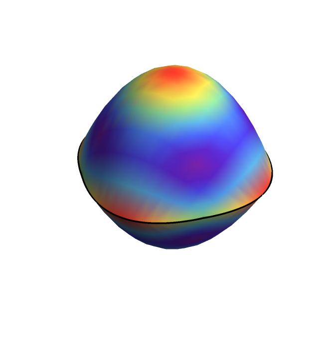
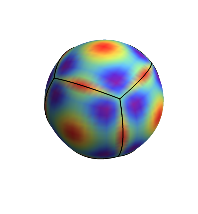
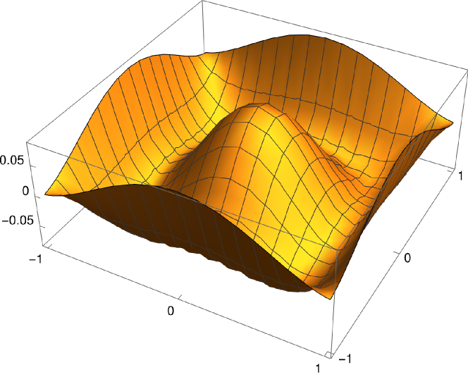
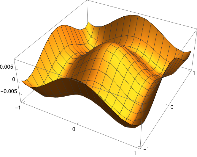
Figure 4: Optimal approximation of the unit sphere by the spline of two tensor product quadratic Bézier patches (upper left) and by the spline of six tensor product quadratic Bézier patches (upper right) together with the graphs of the corresponding radial errors for the single patch (bottom). The colours of the approximants indicate the distance from the sphere (red regions are out of the sphere).

In Table 1, optimal parameters according to the radial error, radial distances and the numerical convergence rates are collected for a set of chosen parameters $a$. The numerical rate of convergence is estimated as follows. Let $d_{1}$ and $d_{2}$ be two consecutive radial distances according to the parameters $a_{1}$ and $a_{2}$. Assuming that the radial distance is of the form $d={\rm const}\,a^{r}$, we can estimate $r\approx\log\left(d_{1}/d_{2}\right)/\log\left(a_{1}/a_{2}\right)$. It is clearly seen that the distance converges to zero as the square of the area of the spherical square.

$a$	$(\alpha_{r}^{*},\beta_{r}^{*})$	$|g|$	$r$
$a_{max}$	$(1.0306,4.3393)$	$8.2331\times 10^{-2}$	$-$
$a_{max}/2$	$(0.5698,1.1630)$	$6.9966\times 10^{-4}$	$6.87$
$a_{max}/4$	$(0.5160,1.0333)$	$3.7421\times 10^{-5}$	$4.23$
$a_{max}/8$	$(0.5039,1.0079)$	$2.2596\times 10^{-6}$	$4.05$
$a_{max}/16$	$(0.5010,1.0020)$	$1.4005\times 10^{-7}$	$4.01$
$a_{max}/32$	$(0.5002,1.0005)$	$8.7349\times 10^{-9}$	$4.00$
$a_{max}/64$	$(0.5001,1.0001)$	$5.4565\times 10^{-10}$	$4.00$

Table 1: Optimal parameters $\alpha_{r}^{*}$ and $\beta_{r}^{*}$ according to the radial error $g$, the corresponding radial distance $|g|$ and the numerical rate of convergence $r$ for several parameters $a=a_{max}/2^{i}$, $i=0,1,\dots,6$, with $a_{max}=1/\sqrt{2}$.

The approximation of the unit sphere by the $G^{1}$ spline of six tensor product quadratic Bézier patches constructed in Section 4 is given in Figure 5. It is clearly seen that its radial error is much bigger than the radial error of the optimal approximant in Figure 4. Moreover, the $G^{1}$ approximant is one-sided, i.e., the whole approximant is out of the sphere. This suggests that omitting the interpolation conditions at the vertices of the spherical square would imply better approximant by pulling it towards the origin.

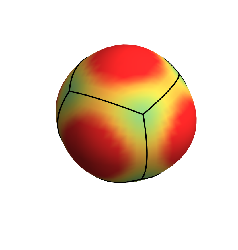
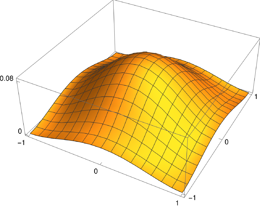
Figure 5: Approximation of the unit sphere by the $G^{1}$ spline of six tensor product quadratic Bézier patches (left) together with the graph of the radial error for the single patch (right). The colours of the spline approximant indicate its distance from the sphere. The red indicates a bigger distance.

7 Conclusion

Finding the optimal polynomial approximant of a given surface is a challenging nonlinear optimization problem. There are only a few references dealing with this problem available. In this paper, we have shown that the results obtained in [1] are not correct. As a counterexample, we found a better approximant of the spherical square and provided an efficient algorithm for its construction. It is natural to consider higher degree polynomial approximants of spherical squares or at least approximants providing smoother polynomial spline patches ($G^{k}$ continuous tensor product spline patches). Both problems might be considered future work, but they lead to much more complicated nonlinear optimisation issues. On the other hand, the approximation of spherical rectangles by tensor product quadratic patches might be of some interest. Preliminary results reveal that, in some cases, it leads to several (infinitely many) optimal solutions. Thus the square and the rectangular case deeply differ in their nature.

Acknowledgments. The first author was supported by the Slovenian Research Agency program P1-0292 and the grant J1-4031. The second author acknowledges financial support from the Slovenian Research Agency program grant P1-0288 and the grants N1-0137 and J1-3005.

References

Eisele [1994]
Eisele, E.F., 1994.
Best approximations of symmetric surfaces by
biquadratic Bézier surfaces.
Comput. Aided Geom. Design 11,
331–343.
Floater [1997]
Floater, M.S., 1997.
An Hermite approximation for conic
sections.
Comput. Aided Geom. Design 14,
135–151.
Grošelj and Šadl
Praprotnik [2022]
Grošelj, J., Šadl Praprotnik, A.,
2022.
Exact sphere representations over Platonic solids
based on rational multisided Bézier patches.
Comput. Aided Geom. Design 98,
Paper No. 102148, 17.
Vavpetič [2020]
Vavpetič, A., 2020.
Optimal parametric interpolants of circular arcs.
Comput. Aided Geom. Design 80,
Paper No. 101891, 9.
Vavpetič and
Žagar [2022]
Vavpetič, A., Žagar, E.,
2022.
Geometric approximation of the sphere by triangular
polynomial spline patches.
Comput. Aided Geom. Design 92,
Paper No. 102061, 12.