A Survey for High-redshift Gravitationally Lensed Quasars and Close Quasars Pairs.
I. the Discoveries of an Intermediately-lensed Quasar and a Kpc-scale Quasar Pair at $z\sim 5$

Abstract

We present the first results from a new survey for high-redshift $(z\gtrsim 5)$ gravitationally lensed quasars and close quasar pairs. We carry out candidate selection based on the colors and shapes of objects in public imaging surveys, then conduct follow-up observations to confirm the nature of high-priority candidates. In this paper, we report the discoveries of J0025–0145 ($z=5.07$) which we identify as an intermediately-lensed quasar, and J2329–0522 ($z=4.85$) which is a kpc-scale close quasar pair. The Hubble Space Telescope (HST) image of J0025–0145 shows a foreground lensing galaxy located $0\farcs 6$ away from the quasar. However, J0025–0145 does not exhibit multiple lensed images of the quasar, and we identify J0025–0145 as an intermediate lensing system (a lensing system that is not multiply imaged but has a significant magnification). The spectrum of J0025–0145 implies an extreme Eddington ratio if the quasar luminosity is intrinsic, which could be explained by a large lensing magnification. The HST image of J0025–0145 also indicates a tentative detection of the quasar host galaxy in rest-frame UV, illustrating the power of lensing magnification and distortion in studies of high-redshift quasar host galaxies. J2329–0522 consists of two resolved components with significantly different spectral properties, and a lack of lensing galaxy detection under sub-arcsecond seeing. We identify it as a close quasar pair, which is the highest confirmed kpc-scale quasar pair to date. We also report four lensed quasars and quasar pairs at $2<z<4$, and discuss possible improvements to our survey strategy.

1 Introduction

Gravitationally lensed quasars are rare and valuable objects that enable important studies in extragalactic astronomy and cosmology. Measuring the time lags between the lensed images of the background quasar gives independent constraints on key cosmological parameters like the Hubble constant (e.g., Wong et al., 2020; Shajib et al., 2020). Microlensing events caused by stars in the lensing galaxy have been used to probe the structure of quasar accretion disks (e.g., Kochanek, 2004; Cornachione et al., 2020). Analyzing the lensing model puts constraints on the properties of dark matter (e.g., Gilman et al., 2020). Measuring the absorption features in the spectra of the lensed quasar images probes the structure of the foreground galaxy’s circumgalactic medium (e.g., Cashman et al., 2021). With the help of lensing magnification, lensed quasars offer unique opportunities to measure the properties of quasars with enhanced sensitivity (e.g., Yang et al., 2019a, 2022) and investigate the small-scale structures in the quasar host galaxies (e.g., Bayliss et al., 2017; Paraficz et al., 2018; Yue et al., 2021b).

Physical pairs of quasars are another population of valuable objects that provide critical information about the evolution of supermassive black holes (SMBHs) and their host galaxies. Quasar pairs with separations of $\gtrsim 100$ kpc have been used to measure the clustering of quasars up to $z\sim 5$ (e.g., McGreer et al., 2016; Eftekharzadeh et al., 2017). Kpc-scale quasar pairs are likely the results of ongoing galaxy mergers, in which the SMBHs in both progenitor galaxies are ignited by the merging event (for a recent review, see De Rosa et al., 2019). Comparison between detailed observations of close quasar pairs (e.g., Green et al., 2010) and zoom-in hydrodynamical simulations of galaxy mergers (e.g., Capelo et al., 2017) helps us to understand how galaxy mergers trigger quasar activities. The statistics of quasar pairs (e.g., the fraction of close pairs among all quasars) encode information about the coevolution of SMBHs, their host galaxies, and their close environments (e.g., Steinborn et al., 2016; Volonteri et al., 2016; Shen et al., 2022).

Given the importance of these objects, there have been intensive efforts to search for gravitationally lensed quasars (e.g., Inada et al., 2012; More et al., 2016; Anguita et al., 2018; Treu et al., 2018; Lemon et al., 2018; Fan et al., 2019; Lemon et al., 2019, 2020) and quasar pairs (e.g., Hennawi et al., 2006, 2010; Silverman et al., 2020; Tang et al., 2021; Chen et al., 2022a). Most of these studies use public imaging surveys such as the Sloan Digital Sky Survey (SDSS; York et al., 2000) to select candidates that have colors and shapes consistent with lensed quasars or quasar pairs, then confirm the nature of the candidates with follow-up spectroscopy and/or high-resolution imaging. Interestingly, the observational features of arcsecond-scale quasar pairs are very similar to that of doubly-imaged lensed quasars with faint lensing galaxies (e.g., Shen et al., 2021). As a result, surveys for lensed quasars naturally lead to discoveries of close quasar pairs (e.g., Lemon et al., 2022) and vice versa (e.g., Chen, 2021).

In the past few years, the Gaia mission (Gaia Collaboration et al., 2016) has revolutionized the searches for lensed quasars and close (arcsecond-scale) quasar pairs. Gaia is an all-sky imaging and spectroscopic survey that primarily aims at mapping the stars in the Milky Way. Using a space-based telescope, Gaia delivers an effective angular resolution of $\sim 0\farcs 4$ in Data Release (DR) 2 (Gaia Collaboration et al., 2018). The astrometric properties measured by Gaia, especially the parallax and proper motions of objects, are useful in identifying lensed quasars and suppressing the contamination of galactic stars (e.g., Lemon et al., 2017). Lemon et al. (2022) show that the number of known of lensed quasars at redshift $z<1.5$ with separations $\Delta\theta>1^{\prime\prime}$ that are detected in the Gaia survey is consistent with model predictions, suggesting a high completeness for Gaia-based lens searches.

Despite the success of previous studies, to date it is still unclear how to efficiently find high-redshift lensed quasars and quasar pairs. Although some lensed quasars at $z\sim 4$ have been discovered using Gaia data (e.g., Desira et al., 2022), most $z\gtrsim 5$ quasars are too faint to be detected in the Gaia survey. In addition, the relatively poor physical resolution of most observations makes it challenging to find kpc-scale quasar pairs at high redshifts. So far, only one lensed quasar has been reported at $z>5$ (Fan et al., 2019) and only one kpc-scale quasar pair has been confirmed at $z>3$ (Tang et al., 2021). These numbers are much lower than predictions from simulations (e.g., Oguri & Marshall, 2010; De Rosa et al., 2019).

In order to draw a comprehensive picture of lensed quasars and quasar pairs, we need to investigate how to efficiently identify faint distant lensed quasars and quasar pairs from imaging surveys. This task is urgent given the upcoming wide-area sky surveys like the Vera C. Rubin Observatory Legacy Survey for Space and Time (LSST; Ivezić et al., 2019) and the Euclid survey (Scaramella et al., 2021). In particular, LSST will deliver imaging that is several magnitudes deeper than Gaia, meaning that Gaia-based survey methods will be less useful in the LSST era.

The above considerations motivate us to design and carry out a new survey for lensed quasars and close quasar pairs, with a focus on high-redshift ones $(z\gtrsim 5)$. We explore strategies that make the most use of current imaging surveys, which can also be applied to upcoming sky surveys like LSST. This paper reports the lensed quasars and close quasar pairs discovered in the initial stage of this survey.

The layout of this paper is as follows. We describe the data sets and the method we use for candidate selection in Section 2. We describe how we confirm the nature of candidates with follow-up observations in Section 3. We then present the discoveries of an intermediately-lensed quasar at $z=5.07$ (J0025–0145, Section 4) and a kpc-scale quasar pair at $z=4.85$ (J2329–0522, Section 5). We also report a few lensed quasars and close quasar pairs at lower redshifts in Section 6. We discuss future work to improve this survey in Section 7. We use a flat $\Lambda$CDM cosmology with $H_{0}=70\text{ km s}^{-1}\text{ Mpc}^{-1}$ and $\Omega_{M}=0.3$.

2 Building the Candidate Sample

This section briefly summarizes the public data sets and the candidate selection method used in our survey. Figure 1 presents a flowchart of the candidate selection pipeline.

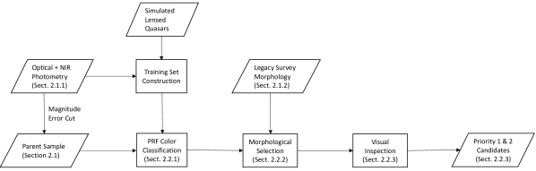
Figure 1: The flowchart of the candidate selection pipeline.

2.1 Data Sets

2.1.1 The Parent Sample and Multi-band Photometry

We construct our parent sample of candidates using a number of optical and infrared sky surveys. The public surveys we use in this work are summarized in Table 1. Specifically, we start with objects in the Dark Energy Survey DR2 (DES; DES Collaboration et al., 2021) and the Pan-STARRS1 survey DR2 (PS1; Chambers et al., 2016). DES covers $\sim 5,000$ deg² of high-galactic-latitude area in the Southern Galactic Cap, providing deep imaging in the $g,r,i,z$ and $Y-$bands. PS1 covers sky areas at $\delta>-30^{\circ}$ with $g,r,i,z$ and $y$-band imaging.

Table 1: Information of Public Surveys Used in the Candidate Selection

Survey	Filters	PSF size	Depth	Reference
		$(^{\prime\prime})$	(mag)
DES	$g,r,i,z,Y$	1.11, 0.95, 0.88, 0.83, 0.90	25.4, 25.1, 24.5, 23.8, 22.4	DES Collaboration et al. (2021)
PS1	$g,r,i,z,y$	1.31, 1.19, 1.11, 1.07, 1.02	23.3, 23.2, 23.1, 22.3, 21.3	Chambers et al. (2016)
VHS	$J,K_{s}$	0.99, 0.91	20.8, 20.0	McMahon et al. (2013)
UKIDSS	$J,H,K$	$<1.2$	19.9, 18.6, 18.2	Lawrence et al. (2007)
UHS	$J$	$<1.2$	19.9	Dye et al. (2018)
WISE	$W1,W2$	6, 6	18,17	Marocco et al. (2021)
Legacy	$g,r,z$	1.29, 1.18, 1.11	23.95, 23.54, 22.50	Dey et al. (2019)
Gaia	$G$	0.4	21	Gaia Collaboration et al. (2018)

Note. — We use the Legacy Survey to gather morphological information of objects, and use Gaia to obtain parallaxes and proper motions of objects. The other surveys are used to obtain the magnitudes of objects.

We obtain near-infrared (NIR) photometry from the Vista Hemisphere Survey (VHS; McMahon et al., 2013), the UKIRT Infrared Deep Sky Survey (UKIDSS; Lawrence et al., 2007), and the UKIRT Hemisphere Survey (UHS; Dye et al., 2018). VHS covers most parts of the southern hemisphere in $Y,J,H$, and $K_{s}$ bands. UKIDSS covers $7,000\text{ deg}^{2}$ in the northern hemisphere with the $Z,Y,J,H$ and $K-$bands, and UHS observes the area at $0^{\circ}<\delta<60^{\circ}$ in $J$ and $K-$bands that are not included in UKIDSS. When we start the candidate selection, UKIDSS finished all the observations, while UHS has only released the $J-$band photometry and VHS has only released the $J$ and $K_{s}-$band photometry for most sky areas. As a result, the exact photometry available for an object depends on its position on the sky. We further obtain the WISE W1 and W2 magnitudes from the CatWISE2020 catalog (Marocco et al., 2021), which is the deepest WISE data release available when the candidate selection was carried out.

Most lensed quasars and kpc-scale quasar pairs have separations of $\lesssim 3^{\prime\prime}$ (e.g., Collett, 2015). To include flux from all the components of these objects, we use aperture magnitudes with a diameter of $5^{\prime\prime}$ in our candidate selection, with the exception of WISE W1 and W2 bands that have PSF sizes of $\sim 6^{\prime\prime}$. We use a matching radius of $2^{\prime\prime}$ when cross-matching the survey catalogs.

We then construct the parent sample of objects by selecting objects at high galactic latitudes with good photometry. The exact criteria are

$$\begin{gathered}|b|>30^{\circ},\\ m_{z}<20,\sigma_{m_{i}}<0.2,\sigma_{m_{z}}<0.1,\\ \sigma_{m_{X}}<0.3,X\in[r,y(Y),J,H,K(K_{s}),W1,W2].\end{gathered}$$ (1)

Here, we do not have requirement on the $g-$band magnitude error, as quasars at $z\gtrsim 5$ have little or no flux at wavelengths bluer than the redshifted Ly$\alpha$ (e.g., Worseck et al., 2014). This parent sample goes into the candidate selection pipeline described in Section 2.2.

We divide the parent sample into point sources and extended sources. For objects in the DES field, we use $\texttt{spread\_model\_z}<0.005$ as the criterion of point sources (e.g., Sevilla-Noarbe et al., 2018); for objects in the PS1 field, the criterion is $\text{{zPSFMag}}-\text{{zApMag}}<0.1$, which is determined using the same approach as Farrow et al. (2014).

2.1.2 Morphological Information

The morphological information of objects is crucial in surveys of lensed quasars and quasar pairs (e.g., Oguri et al., 2006). In this work, we obtain morphological information from the DESI Legacy Imaging Survey (hereafter the Legacy Survey; Dey et al., 2019) DR8. The Legacy Survey provides $g,r$ and $z-$band imaging for $\sim 20,000\text{ deg}^{2}$ of sky areas at $|b|>18^{\circ}$, which is used in the target selection of the Dark Energy Spectroscopy Instrument (DESI; DESI Collaboration et al., 2016). The $z-$band imaging has the sharpest PSF among all the three bands, which has a full-width half maximum (FWHM) of $\sim 1\farcs 1$. Starting from DR8, the Legacy Survey also includes the DES $g,r$, and $z-$band images, reduced using the same Legacy Survey photometric pipeline.

The Legacy Survey measures the magnitudes and the best-fit flux profiles of objects using Tractor (Lang et al., 2016). Tractor is a python-based image fitting and photometry tool. Briefly speaking, Tractor fits the images of an object as a point source and a Sérsic profile, then picks up the best-fit model based on the reduced $\chi^{2}$. Tractor also generates residual images for the best-fit model. The source detection and fitting pipeline can be executed iteratively, i.e., new sources can be detected in the residual image of the previous iteration. In this way, the Legacy Survey can detect faint objects close to a bright object.

The best-fit image models and the residuals provided by Tractor is useful in identifying objects with close companions. Specifically, many lensed quasars and kpc-scale quasar pairs have separations of $\Delta\theta\lesssim 1^{\prime\prime}$ (e.g., Yue et al., 2022a; Shen et al., 2022) and are blended in ground-based images. When fitted as a PSF or a Sérsic profile, these objects will exhibit large image fitting residuals. We thus obtain the residual images of objects and the corresponding reduced $\chi^{2}$ from the Legacy Survey for candidate selection.

2.2 Candidate Selection

The candidate selection method in this work is based on the colors and shapes of objects. Specifically, we first identify objects with colors consistent with a lensed quasar or a quasar pair, then select candidates that have shapes suggestive of lensing structures or close companions.

2.2.1 Color Classification

For each object in the parent sample, we use a probabilistic random forest (PRF; Reis et al., 2019) to predict the probability of the object to be a lensed quasar, a normal galaxy, and a galactic star. Close quasar pairs have colors similar to lensed quasars with faint deflector galaxies and are thus covered by the class of lensed quasars. PRFs are variations of Random Forests (RFs), a class of supervised machine learning algorithm that is widely used in classification and regression. Unlike RFs where the features of data points have no errors, PRFs take the error of features into account by considering each data point as a probabilistic distribution. PRFs are thus the ideal choice for classifying and fitting noisy data.

We construct training sets for galactic stars and normal galaxies using point sources and extended sources from the parent sample. Specifically, we select objects with magnitude errors smaller than 0.1 in all bands as training set objects. We notice that these training sets might contain objects that are not galactic stars or normal galaxies, e.g., quasars and blended pairs of stars. Nevertheless, these objects have little impact on the color classification, as normal stars and galaxies dominate the training sets.

We generate training sets for lensed quasars using simulated quasars and galaxies. We do not use observed lensed quasars due to their limited numbers, especially at high redshifts. Specifically, we use SIMQSO (McGreer et al., 2013) to generate mock quasars at $z>4.5$ following the method in Yue et al. (2022a), and use simulated galaxies from the JAGUAR mock galaxy catalog (Williams et al., 2018) to model the foreground deflector galaxies. We estimate the velocity dispersion $\sigma$ of the simulated galaxies using their stellar mass and Sérsic parameters based on the relation in Bezanson et al. (2011). We then calculate the Einstein radius $\theta_{E}$ of all pairs of mock quasars and simulated galaxies by assuming a Singular Isothermal Sphere (SIS) lensing model,

$$\theta_{E}=4\pi\left(\frac{\sigma}{c}\right)^{2}\frac{D_{\text{ds}}}{D_{\text{s}}}$$ (2)

where $\sigma$ is the velocity dispersion of the galaxy, $D_{\text{s}}$ is the angular diameter distance from the observer to the source, and $D_{\text{ds}}$ is the angular diameter distance from the deflector to the source. In SIS lensing models, the strong lensing cross section of a deflector galaxy is $\pi\theta_{E}^{2}$. Accordingly, we generate mock lensed quasars by randomly drawing 1,000 simulated galaxies as deflectors for each mock quasar using a weight of $\theta_{E}^{2}$.

For the purpose of color classification, we only need the colors of the mock lensed quasars instead of the accurate lensing models. We thus randomly draw a magnification $\mu$ from the distribution $P(\mu)=8/\mu^{3}$ for each mock lensed quasar. This distribution corresponds to SIS deflectors and is a good approximation for galaxy-scale lensing systems (e.g., Yue et al., 2022b). We then calculate the synthetic magnitudes of the lensing system by summing the spectra of the deflector galaxy and the magnified spectra of the background quasar.

Because there are multiple optical and NIR imaging surveys used to construct the parent sample, it is necessary to train several PRFs to account for the differences in filter response curves between the imaging surveys. To be specific, we consider the following combinations of filters that cover all objects in the parent sample:

• PS1 $g,r,i,z,y$ + UHS $J$ + WISE W1, W2

• PS1 $g,r,i,z,y$ + UKIDSS $J,H,K$ + WISE W1, W2

• PS1 $g,r,i,z,y$ + VHS $J,K_{s}$ + WISE W1, W2

• DES $g,r,i,z,Y$ + VHS $J,K_{s}$ + WISE W1, W2

We then randomly draw $10^{6}$ objects from each training set to train the PRFs. We use flux ratios between other bands and the $z-$band as features of the PRFs. We use the PRFs to predict the probabilities for each parent sample object to be a star, a galaxy, or a lensed quasar, and select objects that satisfy

$$P(\text{star})<0.1\text{ and }P(\text{lensQSO})>0.3$$ (3)

This criterion selects non-stellar objects that have some chances to be a lensed quasar. We set a relatively low threshold in $P(\text{lensQSO})$ to include deflector-dominated lensed quasars that may have high $P(\text{galaxy})$ values. Objects selected by this criterion enter the morphological selection described in the following subsection.

2.2.2 Morphological Selection

The second step of the candidate selection is to identify objects that have shapes indicative of a possible lensing structure or close companions. In imaging surveys, lensed quasars and quasar pairs should either be resolved into multiple components, or appear to be one object that cannot be well-described by regular flux profiles (e.g., a PSF and a Sérsic profile). Accordingly, we match the objects that pass the color classification to the Legacy Survey DR8 Tractor catalog using a matching radius of $4^{\prime\prime}$, and select two samples of candidates:

(1) Resolved candidates. For objects that are resolved into multiple components in the Legacy Survey (i.e., with more than one match in the Tractor catalog), we measure the smallest separation between the resolved components $(\Delta\theta_{\text{min}})$ and select objects with $\Delta\theta_{\text{min}}<3^{\prime\prime}$ as candidates. This separation limit is set to reduce the contamination from projected pairs of objects, as most lensed quasars and kpc-scale quasar pairs have separations less than $3^{\prime\prime}$.

(2) Unresolved candidates. We select objects with large $z-$band image fitting reduced $\chi^{2}$ (rchisq_z) as candidates of small-separation (i.e., unresolved) lensed quasars and quasar pairs. Here we use the $z-$band image fitting residual because the $z-$band has a sharper PSF than the $g$ and the $r-$band. We note that the distribution of rchisq_z depends on the magnitudes of objects, as the imperfectness of flux models have higher statistical significance for brighter objects. In this work, we adopt a selection criterion of rchisq_z$>1.55+0.05\times|{\texttt{mag\_z}}-20.5|^{4.5}$, where mag_z is the $z-$band magnitude in the Legacy Survey. This criterion is tuned to include at least 90% of the known lensed quasars (Lemon et al., 2019) in the parent sample. We note that objects with close companions may also be selected into this candidate sample, which allows us to include large-separation lensed quasars that have one component poorly fitted by a single flux profile (e.g., when the lensing galaxy is blended with one of the lensed quasar images).

Table 2 lists the number of candidates that pass each step in the candidate selection. The columns represent different combinations of photometric surveys, as described in Section 2.2.1. About $0.1\%$ of the parent sample candidates pass the color selection and the morphological selection, and the selection efficiency depends on the depth and the seeing of imaging surveys. We visually inspect the selected candidates to identify high-priority ones (Section 2.2.3). We note that the current candidate selection criteria (especially the color selection) are designed to include as many candidates as possible while keeping visual inspection feasible. In the future, the color selection and morphological selection will be improved by adopting new data releases from sky surveys and updating the candidate selection methods, and the visual inspection can be replaced by machine-learning-based methods. More discussions about possible improvements to the candidate selection can be found in Section 7.

Table 2: Number of Candidates Selected in Each Step for Each Subset

	PS1+UKIDSS	PS1+UHS	PS1+VHS	DES+VHS
Parent Sample	12,240,526	22,613,325	27,100,453	29,417,942
Pass Color Selection	52,810	54,290	158,168	78,616
Pass Morphological Selection	17,492(r) + 8,837(u)	11,462(r) + 9,185(u)	19,993(r) + 7,610(u)	11,728(r) + 5,136(u)
Pass Visual Inspection	88 (Priority 1) + 136 (Priority 2)

Note. — Each column in this table correspond to a subset of candidates. The subsets are determined by the photometry used in color selection. For example, the subset “PS1+UKIDSS” contains objects that have photometry from the PS1 and the UKIDSS survey. See Section 2.2.1 for details. Also note that WISE photometry is available for all the candidates.

2.2.3 Visual Inspection

We visually inspect the images and spectral energy distributions (SEDs) of the candidates and subjectively classify the candidates into Priority 1 (likely), Priority 2 (unsure), and Priority 3 (not likely). For resolved candidates, we pay special attention to the fluxes and positions of the resolved components. Objects that contain multiple point sources with similar colors are assigned high priorities, where the point sources may be lensed images of the same quasar or two quasars at the same redshift. For unresolved candidates, if a candidate exhibits the typical features of a quasar, i.e., a power-law SED and bumps in the SED suggesting broad emission lines, it is assigned a high priority. As shown in Table 2, the majority of the visually-inspected candidates are low-priority candidates, which include irregular galaxies, galaxy mergers, pairs of galaxies, pairs of point sources with star-like colors, and pairs of a galaxy and a star-like point source.

We also match the candidate list to the Million Quasar Catalog (Flesch, 2021) to identify known quasars. We assign priority 1 to known quasars that exhibit a lens-like structure or have a companion with similar colors. We further use the parallax and the proper motion from the Gaia DR2 (Gaia Collaboration et al., 2018) to exclude galactic stars. Specifically, if an object has a non-zero parallax $\varpi$, defined as

$$\varpi>3\sigma_{\varpi}$$ (4)

or a non-zero proper motion $\mu$, defined as

$$\mu=\sqrt{\mu_{\alpha}^{2}+\mu_{\delta}^{2}}>3\sqrt{\sigma_{\mu_{\alpha}}^{2}+\sigma_{\mu_{\delta}}^{2}}$$ (5)

the object is rejected from the candidate list. We do not require a candidate to be detected in the Gaia survey.

Note that our candidate sample contains lensed quasars and quasar pairs at low redshifts $(z\lesssim 5)$, though the primary targets of this project are those at high redshifts. In this work, candidates that exhibit features of low-redshift lensed quasars and quasar pairs are also assigned high priorities.

The visual inspection returns 88 priority 1 candidates and 136 priority 2 candidates. We then carry out follow-up imaging and spectroscopy for these candidates to confirm their nature, as described in Section 3. Limited by the telescope resources, we do not observe priority 3 candidates in this project.

We end this Section by briefly discussing the survey completeness. The completeness of color selection is a function of the redshifts and the SEDs of the quasar and, for lensed quasars, the fluxes of the lensing galaxy and the lensing magnification. The morphological selection relies on the image reduction pipeline of the Legacy Survey and the Tractor algorithm, and quantifying their effects on the completeness function is beyond the scope of this paper. The visual inspection further complicates the completeness function. In addition, the completeness function will change as we improve the candidate selection method in the future (Section 7). We thus leave quantitative analyses of the completeness function to subsequent papers and only provide rough estimates here. Our morphology selection is similar to that of the SQLS, which has a completeness of $\sim 50\%$ $(\sim 90\%)$ for simulated lensed quasars with separation $\Delta\theta=0\farcs 8$ $(1^{\prime\prime})$ (Oguri et al., 2006). Previous quasar surveys have reported a high completeness for RF-based color selection ($\gtrsim 95\%$; e.g., Schindler et al., 2018; Khramtsov et al., 2019). We thus expect that the completeness of our color classification and morphological selection is $\gtrsim 80\%$ for marginally-resolved $(\theta\gtrsim 1^{\prime\prime})$ lensed quasars. The completeness of quasar pairs might be higher, as there is no flux contamination from foreground lensing galaxies.

3 Follow-up Observations

In semesters 2021A and 2021B, we successfully observed 66 priority 1 candidates and 10 priority 2 candidates. Generally speaking, we carry out imaging and spectroscopy for each candidate with sufficient spatial resolution, where the candidate is resolved into multiple components. The imaging gives the positions and fluxes of the resolved components, and the spectroscopy reveals if these components are quasars. Depending on the angular sizes of the candidates, the observations may be carried out using ground-based telescopes under good seeing conditions $(\lesssim 0\farcs 7)$, using ground-based telescopes with adaptive optics, or using the Hubble Space Telescope (HST).

We then classify all candidates into four categories based on their images and spectra as follows (also see the discussion in, e.g., Lemon et al., 2022; Chen, 2021):

1. Lensed Quasars: Quadruply-lensed quasars are confirmed if the lensing structure is clearly resolved in the images. For doubly-lensed quasars, we require that the two lensed images are resolved and have similar emission line profiles, and that the lensing galaxy is detected in the image.

2. Physical Quasar Pairs: Physical quasar pairs are confirmed if the two quasars are resolved, have a line-of-sight velocity difference of $\Delta v<2000\text{ km s}^{-1}$ (e.g., Hennawi et al., 2006), and show significant differences in their spectra. We further require that no lensing galaxy is detected in the field. We discuss the meaning of “significant difference” below with more details.

3. Nearly Identical Quasars (NIQs): If a candidate contains two quasar images at the same redshift, but does not meet the criteria for a lensed quasar or a physical quasar pair, the candidate is classified as an NIQ (e.g., Anguita et al., 2018). NIQs may be physical quasar pairs or doubly-lensed quasars with a faint deflector galaxy, and existing data cannot rule out either hypothesis. These objects are referred to as “lensless twins” in Schechter et al. (2017).

4. Contaminants: The main contaminants in this project are emission line galaxies (ELGs), projected pairs of galaxies and stars, and projected pairs of stars. Specifically, the narrow emission lines in ELGs generate features similar to the broad emission lines of quasars in broad-band photometry; late-type stars have long been recognized as the main contaminants in surveys of high-redshift quasars due to their red colors (e.g., Yang et al., 2019b). A few contaminants turn out to be projected pairs of a quasar and a star, or a single quasar without evidence of strong lensing.

To help understand why we adopt the above criteria, it is worth discussing the long-standing problem in distinguishing close quasar pairs and doubly-lensed quasars (e.g., Shen et al., 2021). If a candidate contains two quasar images at the same redshift and no lensing galaxy is detected, we cannot rule out the possibility that the system is a physical quasar pair, even if the two quasar images have nearly identical spectral profiles. Meanwhile, for lensed quasars, microlensing and differential reddening of the lensing galaxy can lead to small differences between the spectra of the lensed images of the same background quasar (e.g., Sluse et al., 2012). An apparent pair of quasars with subtle differences in spectral features might be a doubly-lensed quasar with an undetected deflector (e.g., a heavily obscured galaxy). More discussions can be found in Schechter et al. (2017), Shen et al. (2021) and Yue et al. (2021a).

As such, we require the detection of the deflector galaxy to confirm a doubly-lensed quasar. Low-redshift quasar pairs can be confirmed by detecting their merging host galaxies (e.g., Silverman et al., 2020; Chen et al., 2022b). At higher redshifts, it becomes difficult to detect the quasar host galaxies even with HST (e.g., Yue et al., 2021a). In this case, confirming a physical quasar pair requires significant differences in spectral shapes that cannot be explained by microlensing and differential reddening. Examples of such features include large velocity offsets between emission lines, different broad absorption line (BAL) features, and very different line widths and/or flux ratios. It is still unclear how to confirm a quasar pair if there are only subtle differences in the spectra of the two quasars. In this work, we consider the features of each object individually, which are presented in Section 4 to Section 6.

So far, we have discovered ten lensed quasars and quasar pairs in this survey. Among these objects, three lensed quasars (J0803+3908, J0918–0220, and J1408+0422) were independently reported in Lemon et al. (2022), and one NIQ was reported in our previous paper (J2037–4537 at $z=5.66$; Yue et al., 2021a). In this paper, we report the discoveries of an intermediately-lensed quasar at $z=5.07$ (J0025–0145, Section 4) and a kpc-scale quasar pair at $z=4.85$ (J2329–0522, Section 5). We also mention four lensed quasars and quasar pairs at $z<4$ found in our survey in Section 6. Table 3 summarizes the observations of the lensed quasars and close quasar pairs, and Table 4 lists the properties of these objects. The data are available upon request to the corresponding author. Unless further specified, all the spectra are reduced using PypeIt (Prochaska et al., 2020), and the PSF models of the images are generated using IRAF task psf based on isolated stars in the field.

Table 3: Summary of Observations

Object	Telescope	Instrument	Filter/Grating	$R$	Seeing	$t_{\text{exp}}$
Spectroscopy
J0025–0145	Magellan/Clay Magellan/Clay Magellan/Baade	LDSS3 LDSS3 FIRE	VPH-all VPHBlue Echelle	645 1425 6000	$0\farcs 7$ $0\farcs 7$ $1\farcs 0$	$1\times 600$s $4\times 900$s $1\times 900$s
J0402–4220	Magellan/Clay	LDSS3	VPH-all	645	$0\farcs 7$	$3\times 900$s
J0954–0022	Magellan/Clay	LDSS3	VPH-all	645	$0\farcs 7$	$1\times 600$s
J1051+0334	Magellan/Clay	LDSS3	VPH-all	645	$0\farcs 7$	$3\times 600$s
J1225+4831	LBT	LUCI1	HKSpec	645	$0\farcs 4$	$20\times 60$s
J2329–0522	Magellan/Clay Magellan/Baade	LDSS3 FIRE	VPH-Red Echelle	1357 6000	$0\farcs 7$ 0$\farcs$7	$3\times 1200$s $9\times 909$s
Imaging
J0025–0145	HST	ACS/WFC	F435W F606W	-	$0\farcs 08$ $0\farcs 08$	$4\times 516$s
J0402–4220	Magellan/Clay	LDSS3	$z$	-	$0\farcs 7$	$1\times 60$s
J0954–0022	Magellan/Clay	LDSS3	$z$	-	$0\farcs 7$	$1\times 60$s
J1051+0334	Magellan/Clay	LDSS3	$z$	-	$0\farcs 7$	$1\times 60$s
J1225+4831	LBT	LUCI1	$K$	-	$0\farcs 35$	$2\times 60$s
J2329–0522	Magellan/Clay	LDSS3	$z$	-	$0\farcs 7$	$1\times 30$s

Table 4: Properties of the Lensed Quasars and Quasar Pairs

Object	Redshift	$\Delta\theta$	$N_{gaia}$	Comment	Component	RA	Dec	Magnitude
J0025–0145	5.07	-	1	lensed quasar	Q	00:25:26.83	–01:45:32.48	$m_{\text{F606W}}=20.782\pm 0.001$
					G	00:25:26.79	–01:45:32.51	$m_{\text{F606W}}=21.34\pm 0.03$
J0402–4220	2.88	$1\farcs 27$	1	lensed quasar	Q1	04:02:22.16	–42:20:52.82	$m_{z}=18.948\pm 0.002$
					Q2	04:02:22.06	–42:20:53.44	$m_{z}=20.44\pm 0.02$
					G	04:02:22.08	–42:20:53.40	$m_{z}=20.60\pm 0.03$
J0954–0022	2.27	$1\farcs 21$	1	lensed quasar	Q1	09:54:06.97	–00:22:25.08	$m_{z}=19.92\pm 0.01$
					Q2	09:54:06.96	–00:22:26.28	$m_{z}=21.06\pm 0.04$
					G	-	-	-
J1051+0334	2.40	$0\farcs 99$	0	NIQ	Q1	10:51:32.43	+03:34:17.71	$m_{z}=19.76\pm 0.01$
					Q2	10:51:32.37	+03:34:17.59	$m_{z}=19.82\pm 0.01$
J1225+4831	3.09	$0\farcs 89$	2	NIQ	Q1	12:25:18.62	+48:31:16.15	$m_{K_{s}}=15.77\pm 0.01$
					Q2	12:25:18.63	+48:31:17.03	$m_{K_{s}}=16.88\pm 0.01$
J2329–0522	4.85	$1\farcs 55$	0	quasar pair	Q1	23:29:15.07	–05:22:35.88	$m_{z}=19.95\pm 0.02$
					Q2	23:29:15.18	–05:22:35.96	$m_{z}=20.80\pm 0.04$

Note. — Coordinates and magnitudes are from the best-fit $galfit$ model. The F606W and the $z-$band magnitudes are AB magnitudes, and the $K_{s}-$band magnitudes are Vega magnitudes. The information about the lensing galaxy in J0954-0022 is not included as the parameters do not converge when fitting. See text for details about image fitting.

4 J0025–0145: an Intermediately-Lensed Quasar at $z=5.07$

J0025–0145 was initially reported in Wang et al. (2016) as a luminous quasar with $M_{1450}=-28.63$. The upper panel of Figure 2 shows the images of J0025–0145. The object is modeled as a point source in the Legacy Survey DR8, and the residual image indicates a close companion next to the quasar. J0025–0145 was observed by HST Advanced Camera for Surveys Wide Field Camera (ACS/WFC) in the F435W and F606W bands (Proposal #16460, PI: Yue). In the F606W image, J0025–0145 is resolved into a point source (i.e., the quasar) and an extended source, separated by $0\farcs 60$. The F435W only detects the extended source.

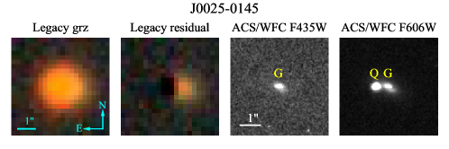
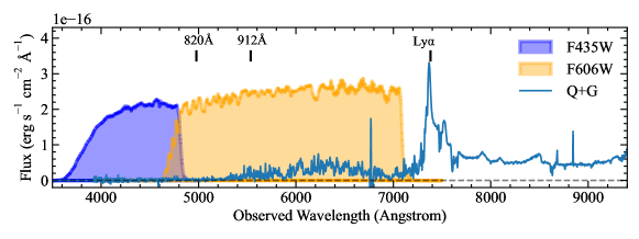
Figure 2: Top: the images of J0025–0145. From left to right: the Legacy Survey $grz$, the Legacy Survey residual, HST ACS/WFC F435W, HST ACS/WFC F606W. J0025–0145 is modeled as a point source in the Legacy Survey, while the residual image indicates a nearby companion. The HST images show the existence of a foreground galaxy. The separation between the quasar and the galaxy is $0\farcs 60$. Bottom: the LDSS3 spectra of J0025–0145. This spectrum is a combination of a VPH-Blue spectrum $(\lambda<5500\text{\AA})$ and a VPH-All spectrum $(\lambda>5500\text{\AA})$. We also plot the response curve of the HST filters and mark the rest-frame wavelengths. The background quasar has no flux at rest-frame $\lambda<820\text{\AA}$, and the F435W image only captures the flux from the foreground lensing galaxy. The F606W image shows both the quasar and the lensing galaxy.

Note that objects at $z>5$ have essentially no flux at rest-frame $\lambda<820\text{\AA}$ due to the absorption of the IGM (e.g., Worseck et al., 2014). The lower panel of Figure 2 shows the spectrum of J0025–0145 taken by the Low Dispersion Survey Spectrograph (LDSS3) on the Magellan/Clay telescope, where we also plot the response curves of the ACS/WFC filters. Since the extended source is detected in the F435W filter, the object must be a foreground galaxy. The small separation between the quasar and the foreground galaxy suggests that the background quasar must be magnified by the galaxy. Interestingly, there is only one point source in the F606W image, meaning that the background quasar is not multiply-imaged. We thus report J0025–0145 as an intermediate lensing system, i.e., lensing systems that do not have multiple images but have a significant magnification, in contrast with weak and strong lensing (e.g., Mason et al., 2015).

To further investigate the structure of J0025–0145, we fit the F606W image by a PSF plus a Sérsic profile using galfit (Peng et al., 2002). The result is presented in Figure 3. The foreground galaxy has a high ellipticity of $e=1-b/a=0.53$. Deflectors of such high ellipticities can generate large magnifications $(\mu\gg 2)$ without producing multiple images of the source (e.g., Keeton et al., 2005). Also note that the residual image shows irregular structures in the galaxy, suggesting a complex mass profile for the deflector galaxy.

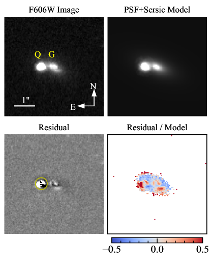
Figure 3: The galfit model of J0025–0145. Top left: the HST ACS/WFC F606W image; Top right: the model image (one PSF and one Sérsic profile); Bottom left: the residual image; Bottom right: the relative residual map. There is no evidence for a second lensed image of the background quasar. The deflector galaxy has a high ellipticity $(e=0.53)$ and exhibit irregular structures. The quasar shows positive flux in the residual image, which cannot be explained by PSF inaccuracies and thus indicates a detection of the quasar host galaxy (see text for details). The residual flux in the yellow aperture (diameter $0\farcs 6$) is $m_{\text{F606W}}=24.2$.

Another noticeable feature is the positive flux residual around the quasar. The lower right panel of Figure 3 shows the relative difference between the model and the real image. The relative difference reaches $\gtrsim 50\%$ for the regions with positive residual flux, which is much higher than the PSF variances in ACS/WFC images ($\lesssim 3\%$ for individual pixels; e.g., Bellini et al., 2018). Using an aperture of $0\farcs 6$ centered at the quasar’s position (marked by the solid yellow circle in Figure 3), we estimate the residual flux to be $m_{\text{F606W}}=24.2$, i.e., about 4.4% of the total quasar flux. In comparison, the $5-\sigma$ magnitude limit for this aperture is $m_{\text{F606W}}=25.8$.

The most plausible scenario is that the positive flux comes from the emission of the quasar host galaxy. Lensing magnification increases the angular size of the host galaxy, making it easier to get detected. Moreover, some regions in the galaxy might have large magnifications up to infinity. Detecting the rest-frame UV emission from quasar host galaxies at $z\gtrsim 5$ has never been successful with HST and is very difficult even with the James Webb Space Telescope (JWST) (e.g., Marshall et al., 2020; Ding et al., 2022). J0025–0145 illustrates the power of lensing magnification in the studies of high-redshift quasar host galaxies.

We note that naked-cusp lenses can generate multiply-imaged lensing systems with infinitely small lensing separation (e.g., Fujimoto et al., 2020). We thus consider the possibility that J0025–0145 is a naked-cusp lens with a tiny lensing separation. Specifically, we use a Singular Isothermal Ellipsoid (SIE) deflector plus an external shear to model the lensing potential, where we fix the ellipticity of the SIE to be $e=0.53$. Note that we are not able to fit the HST image due to the limited spatial resolution; instead, we tune the model parameters to test if we can reproduce systems that resemble the features of J0025–0145.

We find that, in order to generate compact lensing systems with lensing separations $\Delta\theta\lesssim 0\farcs 1$, we need a large external shear $(\gamma\gtrsim 0.1)$ and fine-tuning of the source position. In addition, such models always generate positive flux residuals at the north or south side of the quasar, which is inconsistent with the HST images where the flux residual lies on the east side (Figure 3). We thus conclude that the naked-cusp lensing model is disfavored by existing data.

With only one image of the background quasar, we are not able to build the lensing model and reconstruct the source plane emission for J0025–0145. Instead, we use the apparent Eddington ratio $(\lambda_{\text{Edd}})$ of J0025–0145 to estimate its lensing magnification. Specifically, the Eddington ratio follows the relation $\lambda_{\text{Edd}}\propto L_{\text{bol}}/M_{\text{BH}}$, where $L_{\text{bol}}$ is the bolometric luminosity of the quasar. The SMBH mass, $M_{\text{BH}}$, is usually measured using broad emission line widths and continuum luminosities (e.g., Vestergaard & Osmer, 2009):

$$M_{\text{BH}}=10^{\text{zp}}\left(\frac{\text{FWHM}}{1000\text{ km s}^{-1}}\right)^{2}\left(\frac{\lambda L_{\lambda}}{10^{44}\text{ erg s}^{-1}}\right)^{0.5}$$ (6)

The scaling factor, $10^{\text{zp}}$, depends on the exact line used in the measurement. For lensed quasars, lensing magnification changes the luminosities $(L_{\text{bol}}$ and $\lambda L_{\lambda})$ but does not influence the line width. Combining the above relations gives $\lambda_{\text{Edd}}\propto\mu^{0.5}$, i.e., the observed Eddington ratio is higher than the intrinsic value if the lensing magnification is not corrected.

We use the Mg ii emission line to measure the SMBH mass for J0025–0145. The left panel of Figure 4 shows the Mg ii line of J0025–0145 taken by the Folded-port InfraRed Echelle (FIRE) on the Magellan/Baade telescope. We fit the region around the Mg ii line using a power-law continuum plus a single Mg ii line and a series of Fe ii lines. We use the Fe ii line template from Tsuzuki et al. (2006) and use Gaussian functions to describe the profiles of emission lines. The best-fit model gives $\text{FWHM}_{\text{Mg\,{\sc ii}}}=1798\pm 37\text{ km s}^{-1}$ and $L_{3000}=1.56\times 10^{47}\text{ erg s}^{-1}$. Using the relation in Vestergaard & Osmer (2009), we estimate the black hole mass to be $M_{\text{BH}}=9.24\times 10^{8}M_{\odot}$ without correcting the magnification effect. The error of $M_{\text{BH}}$ is about 0.55 dex and is dominated by the scatters of the empirical relation (Equation 6). We estimate the bolometric luminosity using the bolometric correction suggested by Runnoe et al. (2012), which gives $L_{\text{bol}}=8.26\times 10^{47}\text{ erg s}^{-1}$.

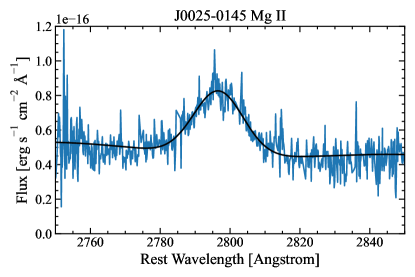
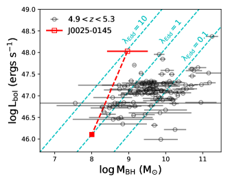
Figure 4: Left: the Mg ii line of J0025–0145, taken by the Magellan/Baade FIRE spectrograph. We fit the region around the Mg ii line as a power law plus a Gaussian profile and a series of Fe ii lines. The best-fit model gives $\text{FWHM}_{\text{Mg\,{\sc ii}}}=1798\pm 37\text{ km s}^{-1}$, using which we calculate the SMBH mass of J0025–0145 to be $M_{\text{BH}}=9.24\times 10^{8}M_{\odot}$ (before correcting for the magnification effect). See text for details. Right: the $M_{\text{BH}}-L_{\text{bol}}$ distribution of quasars. The red open square marks the apparent values (i.e., without correcting for the lensing magnification) of J0025–0145, and the gray circles represents SDSS DR16 quasars at $4.9<z<5.3$ from Wu & Shen (2022). Cyan dashed lines mark constant Eddington ratios. Most quasars have Eddington ratios smaller than or consistent with one, while J0025–0145 has a large apparent Eddington ratio of $\lambda_{\text{Edd}}=9$. The red dashed line illustrates how lensing magnification moves a quasar in this diagram. A magnification of $\mu=84$ is needed to move J0025–0145 onto the line of $\lambda_{\text{Edd}}=1$ (the filled red square).

The right panel of Figure 4 shows the distribution of SMBH masses and bolometric luminosities of quasars at $4.9<z<5.3$ from the SDSS DR16 quasar catalog (Wu & Shen, 2022). The median Eddington ratio of these quasars is 0.4, and most quasars have Eddington ratios consistent with or smaller than one. In contrast, J0025–0145 has a high apparent Eddington ratio of $\lambda_{\text{Edd}}=9$ before correcting for lensing magnification. Again, the error of $\lambda_{\text{Edd}}$ is 0.55 dex and is dominated by the scatters of Equation 6. Assuming that the quasar has an intrinsic Eddington ratio of $\lambda_{\text{Edd}}=1$ (i.e., Eddington-limit accretion), we need a magnification of $\mu=84$. Even if J0025–0145 is accreting at a super-Eddington rate of $\lambda_{\text{Edd}}\approx 3$, we still get a magnification of $\mu\approx 9$.

We notice that the estimation above is subject to several systematic uncertainties, in particular the errors in the SMBH mass measurement and in the bolometric correction. Nevertheless, the result indicates that J0025–0145 has a high magnification of $\mu\gg 1$. Future observations with the Atacama Large Millimeter/Submillimeter Array will characterize the lensed arc of the quasar host galaxy, enabling accurate lens modeling of this system. If the high magnification is confirmed by the lensing model, J0025–0145 will offer unique opportunities to investigate a distant quasar host galaxy with high spatial resolution.

5 J2329–0522: a Kpc-scale Quasar Pair at $z=4.85$

Figure 5 shows the images and spectra of J2329–0522. In the Legacy Survey DR8, J2329–0522 is modeled as a de Vaucouleurs profile, and the large image fitting residual suggests that the flux model is incorrect. J2329–0522 was observed using LDSS3 in both imaging mode and spectroscopy mode under a seeing of $\sim 0\farcs 7$. The LDSS3 $z-$band image is well-described by two point sources, showing no signs of a lensing galaxy in the field. The two point sources are separated by $1\farcs 55$. The lower panel of Figure 5 shows the spectra of the two point sources, both of which exhibit features of quasars at $z=4.85$. The NIR part $(\lambda>1\mu\text{m})$ of the spectra was taken with FIRE. The two components have different spectral shapes, with the fainter component (Q2) being redder. The broad emission line profiles of the two components also show significant differences. In particular, Q1 has a prominent C iii] line, which is nearly absent in the spectrum of Q2. The C iv profiles of the two components also look different.

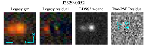
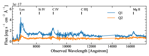
Figure 5: Top: the images of J2329–0522. From left to right: the Legacy Survey $grz$ image, the Legacy Survey residual, the LDSS3 $z-$band image, the two-PSF residual of the LDSS3 image. J2329–0522 is modeled as a de Vaucouleurs profile in the Legacy Survey DR8. The two-PSF residual of the LDSS3 image shows no evidence of a foreground lensing galaxy. Bottom: the spectra of J2329–0522. These spectra are combinations of LDSS3 VPH-Red spectra $(\lambda<1\mu\text{m})$ and FIRE Echelle spectra $(\lambda>1\mu\text{m})$. The emission line profiles of the two quasars show significant differences, and we classify this object as a physical quasar pair (see text for details).

To further investigate the possibility of J2329–0522 being a doubly-lensed quasar, we fit the Si iv, C iv, C iii] lines using a power-law continuum plus a Gaussian profile. We also fit the Mg ii lines using the method described in Section 4. Figure 6 presents the result, and Table 5 summarizes the best-fit parameters. The Mg ii and the Si iv redshifts of Q2 are higher than that of Q1, while Q2 has a lower C iv redshift than Q1. There is a $2.8\sigma$ difference between the FWHM of the C iv lines of the two components. The C iii] line of Q2 is only marginally detected, and the C iii] equivalent width (EW) of Q1 is about six times larger than that of Q2. Meanwhile, the EWs of the two C iv lines only differ by $\sim 50\%$. It is implausible that the FWHM and EW differences between the two quasars in J2329–0522 are results of microlensing. For instance, Sluse et al. (2012) report the microlensing effect of 17 lensed quasars, where the microlensing magnification of different broad emission lines are similar. Also, note that differential reddening has no impact on the FWHM and EW of emission lines.

We thus conclude that J2329–0522 is a physical quasar pair. The projected separation is 9.88 kpc at $z=4.85$, and J2329–0522 is the first quasar pair with projected separation $\Delta d<10$ kpc confirmed at $z>3.2$. The mass ratio of the two SMBHs is close to unity, which is similar to J2037–4537 (an NIQ at $z=5.66$) reported in Yue et al. (2021a) and is consistent with the prediction of hydrodynamical simulations (e.g., Capelo et al., 2017). The small separation between the two quasars suggests that the two quasar host galaxies are in the progress of merging. According to the analysis in Yue et al. (2021a), the clustering of quasars cannot explain the existence of kpc-scale quasar pairs at $z\sim 5$. As such, the two quasars in J2329–0522 are likely triggered by the ongoing galaxy merger.

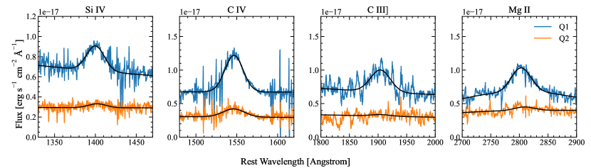
Figure 6: The Si iv, C iv, C iii], and Mg ii lines of J2329–0522. We fit the lines as a power-law continuum and a Gaussian profile emission line, except for the Mg ii line where we add a series of Fe ii lines. The best-fit models are demonstrated by the black lines, and the best-fit parameters are listed in Table 5. These emission lines show vastly different EW ratios between the two quasars, which is difficult to be explained by microlensing. In particular, the C iii] line is prominent in Q1 but is only marginally detected in Q2. In addition, the two quasars show a $2.8\sigma$ difference in the C iv FWHM. These features suggest that J2329–0522 is a physical pair of quasars instead of a doubly-lensed quasar.

Table 5: Emission Line Properties of J2329–0522

Component	Q1	Q2
Si iv line
Redshift	$4.8643\pm 0.0011$	$4.8725\pm 0.0062$
FWHM $(\text{km s}^{-1})$	$5506\pm 156$	$5421\pm 887$
EW (Å)	$60\pm 2$	$21\pm 4$
C iv line
Redshift	$4.8410\pm 0.0005$	$4.8396\pm 0.0023$
FWHM $(\text{km s}^{-1})$	$5099\pm 65$	$6034\pm 332$
EW (Å)	$132\pm 2$	$77\pm 6$
C iii] line
Redshift	$4.8363\pm 0.0030$	[4.8363]
FWHM $(\text{km s}^{-1})$	$6449\pm 416$	[6449]
EW (Å)	$123\pm 10$	$18\pm 4$
Mg ii line
Redshift	$4.857\pm 0.001$	$4.868\pm 0.005$
FWHM $(\text{km s}^{-1})$	$4549\pm 103$	$4586\pm 580$
EW (Å)	$246\pm 5$	$46\pm 6$
Other Properties
$\log(M_{\text{BH, MgII}}/M_{\odot})$	9.49	9.42
$M_{1450}$	-26.1	-25.1
$M_{3000}$	-27.5	-27.1

Note. — The fit does not converge for the C iii] line of Q2 if we keep all parameters free. We thus fix the FWHM and the central wavelength to the best-fit values of Q1 when fitting the C iii] line of Q2.

6 Low-redshift Lensed Quasars and Quasar Pairs

In this Section, we present the low-redshift $(z<4)$ lensed quasars and quasar pairs found in our survey.

6.1 J0402–4220: a lensed quasar at $z=2.88$

Figure 7 shows the images and spectra of J0402–4220. J0402–4220 is modeled as a point source in the Legacy Survey DR8, and the residual image indicates the existence of a close companion. J0402–4220 was observed using LDSS3 in both imaging and spectroscopic mode. Under a seeing of $\sim 0\farcs 7$, J0402–4220 is clearly resolved into two components separated by $1\farcs 27$. The two traces exhibit broad emission lines at the same redshift, $z=2.88$, and the line profiles are similar. This feature suggests that J0402–4220 is a doubly lensed quasar.

To test the strong-lensing scenario, we fit the LDSS3 $z-$band image as two PSFs. The residual image clearly shows a lensing galaxy lying between the two PSF components, which confirms J0402–4220 as a lensed quasar. We also fit the image as two PSFs plus a de Vaucouleurs profile, and the best-fit de Vaucouleurs profile has a half-light radius of $R_{e}=0\farcs 37$ and an axis ratio of $q=0.23$. The small radius and the extreme axis ratio indicate that the lensing galaxy is only marginally resolved in the image. Since the ellipticity of the deflector might be inaccurate, we do not carry out lens modeling for J0402–4220 in this paper. J0402–4220 was also reported by Lemon et al. (2020) as an inconclusive candidate, where this object was modeled as a quasar blended with a galaxy without decisive features of strong lensing.

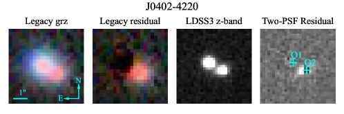
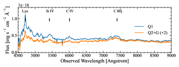
Figure 7: Top: the images of J0402–4220. From left to right: the Legacy Survey $grz$ image, the Legacy Survey residual image, the LDSS3 $z-$band image, the two-PSF residual of the LDSS3 image. J0402-4220 is modeled as a point source in the Legacy Survey DR8. The two-PSF residual of the LDSS3 image shows another source between the two point sources, i.e., the lensing galaxy. Bottom: the LDSS3 spectra of J0402-4220, clearly showing that the two components are two quasars at the same redshift, $z=2.88$. The spectrum of the fainter component (Q2+G) is scaled by a factor of two.

6.2 J0954–0022: a lensed quasar at $z=2.27$

J0954–0022 (Figure 8) was initially reported by Croom et al. (2001) as a luminous quasar. The Legacy Survey image indicates that J0954–0022 consists of two components with similar colors. J0954–0022 was observed using LDSS3 under a seeing of $\sim 0\farcs 7$. In the LDSS3 $z-$band image, J0954–0022 is resolved into two components with a separation of $1\farcs 21$. The broad emission line profiles of the two components are nearly identical.

We fit the LDSS3 image as two PSFs, and the fitting residual show a faint lensing galaxy lying between the two PSFs. We thus confirm J0954–0022 as a lensed quasar. We also try to add a de Vaucouleurs profile or an exponential profile to the model, but the fitting does not converge. We argue that the current image does not have sufficient spatial resolution and/or depth to characterize the foreground lensing galaxy, and we do not perform lens modeling for J0954–0022.

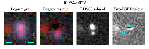
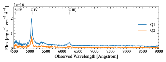
Figure 8: Same as Figure 7, but for J0954–0022. J0954-0022 is modeled as a single point source in the Legacy Survey DR8. The two-PSF residual of the Legacy Survey image shows the existence of a lensing galaxy, and the spectra of both components exhibit features of a quasar at $z=2.27$.

6.3 J1051+0334: a lensed quasar at $z=2.40$

Figure 9 shows the images and spectra of J1051+0334. J1051+0334 was observed using LDSS3 under a seeing of $\sim 0\farcs 6$. In the LDSS3 $z-$band image, J1051+0334 is resolved into two components with a separation of $0\farcs 99$. The spectroscopy shows that both components are heavily reddened BAL quasars at $z=2.40$. The emission line profiles and the BAL features of the two components are similar, while quasar Q1 shows stronger emission lines than quasar Q2.

The LDSS3 $z-$band image of J1051+0334 can be well-fitted by two PSFs, and no foreground lensing galaxy is detected. However, it is extremely unlikely to have a close pair of BAL quasars exhibiting spectra so similar to each other. The difference in the emission line strengths can be explained by microlensing effect on the broad line region. We thus classify this object as a lensed quasar. A similar case is reported in Hutsemékers et al. (2020).

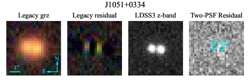
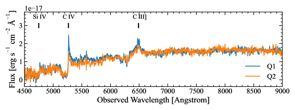
Figure 9: Same as Figure 7, but for J1051+0334. J1051+0334 is modeled as a Sérsic profile in the Legacy Survey DR8. The spectra of both components exhibit features of a BAL quasar at $z=2.40$. The emission line shapes of the two components are similar, while Q1 has larger emission line fluxes than Q2. Although we do not see clear evidence of a lensing galaxy in the two-PSF residual of the LDSS3 image, the nearly identical BAL features suggest that J1051+0334 must be a lensed quasar.

6.4 J1225+4831: an NIQ at $z=3.09$

J1225+4831 was initially reported in Schindler et al. (2018) as a luminous quasar and was selected as a grade A candidate of lensed quasars and quasar pairs in Dawes et al. (2022). J1225+4831 was observed using the Large Binocular Telescope (LBT) LUCI1 in both imaging and spectroscopic mode. We enabled the Enhance Seeing Mode (ESM) in the observing runs, which delivered a PSF size of $\sim 0\farcs 35$. The images and spectra are shown in Figure 10. In the LUCI1 $K-$band image, J1225+4831 is clearly resolved into two point sources separated by $0\farcs 89$. The LUCI1 spectra show that both components exhibit features of a quasar at $z=3.095$.

As a side effect of the ESM observation, the PSF of the LUCI1 image depends on the position on the image. Consequently, we cannot use field stars to construct the PSF model. To test if J1225+4831 can be well-described by two point sources, we fit the image as two Moffat profiles, where we force the two components to have the same profile. The residual is shown in Figure 10, which does not exhibit signs of a lensing galaxy.

We notice that the line profiles of the two components in J1225+4831 are different; specifically, the H$\beta$ peak of Q1 is higher than the [O iii] peak, while for Q2, the peaks of the two lines are close. This difference can be explained by microlensing effect on the broad line region. We thus classify this object as an NIQ.

J1225+4831 is an extremely luminous quasar with $m_{r}=17.9$ (PS1). We thus test the possibility that the high luminosity of J1225+4831 is a result of lensing magnification. Following the argument in Section 4, if J1225+4831 is a lensed quasar, the apparent Eddington ratio estimated using the total spectrum (i.e., the sum of components A and B) will be $\mu^{0.5}$ times the intrinsic Eddington ratio. We thus fit the total spectrum as a power law plus three Gaussian profiles, which represent the H$\beta$, the [O iii]4959Å, and the[O iii]5007Å line, respectively. We fix the flux ratio of the [O iii]5007Å line and the [O iii]4959Å line to be 3 and require the two lines to have the same redshift and FWHM. This fitting gives $\text{FWHM}_{\text{H}\beta}=7130\text{ km s}^{-1}$ and $L_{5100\text{\AA}}=4.56\times 10^{46}\text{ erg s}^{-1}$. Using the SMBH mass estimator given by Vestergaard & Peterson (2006) and the bolometric correction given by Runnoe et al. (2012), we estimate the apparent Eddington ratio of J1225+4831 to be 0.3. This apparent Eddington ratio is not indicative of a large lensing magnification.

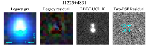
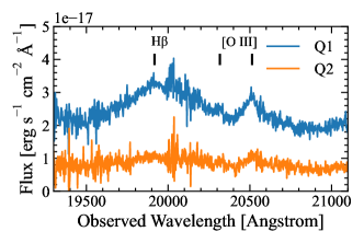
Figure 10: Top: the images of J1225+4831. From left to right: the Legacy Survey $grz$, the Legacy Survey residual, the LBT/LUCI1 $K-$band image, the two-PSF residual of the LUCI image. J1225+4831 is modeled as two PSFs in the Legacy Survey DR8. The $K-$band image has a PSF FWHM of $0\farcs 35$, and is well-fitted by two PSFs. Bottom: the LBT/LUCI1 HKspec spectrum of the two components, showing that both components are a quasar at $z=3.09$.

7 Discussions and Future Work

In this work, we present six lensed quasars and quasar pairs discovered in the initial stage of our survey. In addition to these objects, we have also independently found three lensed quasars that are reported earlier in Lemon et al. (2022) and one NIQ that is reported in Yue et al. (2021a). We thus estimate the current survey efficiency to be $10/76\approx 13\%$. All these objects are Priority 1 candidates; if we count Priority 1 candidates only, the efficiency is $10/66\approx 15\%$. Recent Gaia-based surveys for lensed quasar and close quasar pairs have efficiencies of $\sim 30\%$ (e.g., Lemon et al., 2020; Chen et al., 2022a). Since our survey includes faint candidates that are not detected in Gaia, a selection efficiency of $\sim 15\%$ is reasonable.

The candidate selection method of this work relies on the colors and shapes of objects, which is similar to the approach of the SQLS (e.g., Oguri et al., 2006; Inada et al., 2012). There are two major differences between the SQLS and this work. First, the parent sample of SQLS consists of spectroscopically confirmed SDSS quasars, while this work uses color-selected quasar candidates. By applying relatively loose color selection criteria, we can include lensed quasars with bright deflector galaxies. Second, the morphological selection in the SQLS identifies quasars that cannot be well-described by PSFs, while in this work, we select objects that can be well-fitted by neither PSFs nor Sérsic profiles. The more strict morphological selection of this work reduces the contamination from regular galaxies, resulting in a viable number of candidates for visual inspection.

Recent searches for lensed quasars and close quasar pairs heavily rely on the Gaia survey, which offers high spatial resolution $(0\farcs 4)$ and high-precision parallax and proper motion measurements. Techniques used in these studies include (1) searching for quasars that have multiple matches in the Gaia catalog (e.g., Agnello, 2017; Ducourant et al., 2018); (2) selecting quasars that have abnormal astrometry (e.g., Lemon et al., 2017; Chen et al., 2022a); (3) selecting quasars that show differences between Gaia photometry and ground-based photometry (e.g., Lemon et al., 2017).

Since the primary targets of our survey are quasar pairs and lensed quasars at $z\gtrsim 5$, in this work, we do not require candidates to be detected in Gaia. The reason is that Gaia mainly covers the optical wavelengths, while high-redshift quasars have little flux at the blue side of Ly$\alpha$ due to IGM absorption. Candidate selection methods based on object colors and morphology help us to find lensed quasars and quasar pairs beyond the flux limit of Gaia. Indeed, three quasar pairs and NIQs discovered in our survey (J1051+0334, J2329–0522, and J2037–4537) are not detected in Gaia DR3.

In the future, we will adopt new data releases from public surveys (e.g., the Legacy Survey DR9 and the Gaia survey DR3) and improve the candidate selection method. In particular, some candidates are resolved into multiple components in the Legacy Survey, though the survey catalog incorrectly describes the candidates as single-component objects. J2329–0522 (Figure 5), J0402–4220 (Figure 7), J0954–0022 (Figure 8), and J1051+0334 (Figure 9) are all examples of such cases. It is thus useful to reprocess the images of candidates using optimal source deblending algorithms, which will provide the flux of the resolved components. We note that one major source of contaminants is projected pairs of objects (e.g., galaxy+galaxy, galaxy+star, star+star, and quasar+star). Reprocessing the images from public surveys will help us to get accurate SEDs of the resolved components and to exclude projected pairs of objects in the color selection.

Another critical improvement to make is to develop automatic algorithms in place of visual inspection. For example, neural networks have been found useful in finding lensed galaxies (e.g., Lanusse et al., 2018) as well as quadruply-lensed quasars (e.g., Akhazhanov et al., 2022). However, the application of deep learning in searching for high-redshift lensed quasars and quasar pairs has been poorly explored. Developing these algorithms is necessary to handle the large candidate sample from the LSST and the Euclid survey, as well as to estimate the survey completeness and correctly analyze the statistics of lensed quasars and quasar pairs found in this survey.

8 Summary

We present the first results from a new survey for high-redshift lensed quasars and close quasar pairs. The candidate selection is based on broad-band photometry from a number of public imaging surveys and morphological information from the Legacy Survey DR8. We use PRF classifiers to identify objects that have colors consistent with a lensed quasar or a quasar pair. We further select objects that have close companions or have large image fitting residuals in the Legacy Survey as candidates. We visually inspect the candidates and carry out follow-up imaging and spectroscopy for high-priority ones.

In semesters 2021A and 2021B, we observed 66 priority 1 candidates and 10 priority 2 candidates, from which we independently discovered ten lensed quasars and close quasar pairs. Three out of ten objects discovered in this survey are not detected in Gaia. In this paper, we highlight J0025–0145 at $z=5.07$ (an intermediately-lensed quasar) and J2329–0522 at $z=4.85$ (the most distant close quasar pair reported so far). The HST images of J0025–0145 indicate a tentative detection of the quasar host galaxy, with the help of lensing magnification and distortion. We also mention four lensed quasars and NIQs at $z<4$ that are not reported by previous studies.

In the future, we will improve our survey by adopting new data releases from public sky surveys and updating the candidate selection method. We will also develop automatic tools (e.g., deep-learning-based algorithms) in place of the visual inspection. Upcoming wide-area sky surveys like LSST and Euclid will provide unprecedented depth and spatial resolution and probe compact lensing systems and sub-kpc quasar pairs, which are largely unexplored so far (e.g., Chen et al., 2022a). The methods used in this work can be adapted and applied in these future imaging surveys.

Appendix A Information of Candidates with Follow-Up Spectroscopy

Here we summarize all objects with follow-up spectroscopy. The spectral types of the objects are determined by visual inspection. Specifically, if an object exhibits multiple broad emission lines, we confirm the object as a quasar and determine its redshift. An object is reported as a galaxy if it appears to be extended in images and has a spectrum consistent with a galaxy. We determine the redshift of the galaxy only if there are prominent emission lines. Similarly, an object is reported as a star if it appears to be a point source in images and has a spectrum consistent with a star. We do not determine the specific spectral types of stars. If we cannot determine the type of the spectrum (usually due to insufficient S/N), we report the object as inconclusive. The spectra are available upon request to the corresponding author.

Table 6: Candidates with Follow-Up Spectroscopy

Name	RA	Dec	Priority	Spectral Type	Comment
J0025–0145	00:25:26.83	–01:45:32.51	1	Quasar	Intermediately lensed, $z=5.07$
J0032+0120	00:32:18.14	+01:20:36.30	1	Galaxy
J0054+0133	00:54:00.42	+01:33:52.46	1	Star	May be two stars blended
J0101+0034	01:01:31.34	+00:34:12.07	1	Star	May be a star and a galaxy blended
J0109–0524	01:09:13.82	–05:24:01.52	1	Inconclusive	No trace
J0118–1915	01:18:44.60	–19:15:02.57	1	Star	May be a star and a galaxy blended
J0124+0553	01:24:09.69	+05:53:43.06	1	Star + Galaxy
J0125+0142	01:25:21.41	+01:42:17.21	1	Star	May be two stars and a galaxy blended
J0127–0701	01:27:48.00	–07:01:07.84	1	Star
J0133–5804	01:33:07.19	–58:04:26.91	1	Quasar + Inconclusive	Quasar at $z=3.08$
J0134–2308	01:34:57.48	–23:08:54.57	1	Star
J0151–2242	01:51:41.26	–22:42:09.43	1	Star + Galaxy
J0154–0250	01:54:56.09	–02:50:54.87	1	EmGal	$z=0.39$
J0158+1541	01:58:03.99	+15:41:50.08	1	Star
J0205+0357	02:05:01.41	+03:57:07.02	1	Star + Galaxy
J0212–1548	02:12:34.63	–15:48:21.45	1	Quasar	$z=4.75$, no sign of lensing
J0223–4709	02:23:06.75	–47:09:02.72	1	Quasar	$z=5.0$, no sign of lensing
J0234–0652	02:34:15.83	–06:52:08.58	1	Star + Galaxy
J0240–0019	02:40:25.00	–00:19:36.52	1	Star	Two stars blended but unresolved in the spectrum
J0256–1817	02:56:29.09	–18:17:27.37	1	AGN + Star	AGN at $z=1.22$
J0307–0108	03:07:15.57	–10:18:28.47	1	Galaxy
J0311–2343	03:11:54.69	–23:43:24.18	1	Galaxy + Star
J0315–1710	03:15:33.62	–17:10:05.34	1	Quasar	$z=2.79$, no sign of lensing
J0348–0438	03:48:37.24	–04:38:14.26	1	Galaxy
J0352–2145	03:52:10.62	–21:45:45.03	1	Quasar	$z=5.1$, no sign of lensing
J0402–4220	04:02:22.13	–42:20:53.03	1	Quasar	Lensed, $z=2.88$
J0408–6442	04:08:49.69	–64:42:32.41	1	Star
J0449–3143	04:49:43.33	–31:43:04.13	1	Quasar + Inconclusive	Quasar at $z=2.07$, blended with a star-like point source
J0453–6059	04:53:33.73	–60:59:54.79	1	Star
J0504–3311	05:04:40.51	–33:11:05.75	1	Inconclusive	May be a FeLoBAL
J0527–2958	05:27:50.65	–29:58:52.23	1	Star
J0532–3005	05:32:20.43	–30:05:22.33	1	AGN	$z=0.36$
J0803+3908	08:03:57.75	+39:08:23.06	1	Quasar	Lensed $(z=2.98)$, also reported in Lemon et al. (2022)
J0841+2804	08:41:19.99	+28:04:01.82	1	Star
J0846+2752	08:46:00.51	+27:52:43.06	1	Star
J0848+2630	08:48:34.94	+26:30:42.77	1	Star
J0918–0220	09:18:43.37	–02:20:07.41	1	Quasar	Lensed $(z=0.8)$, also reported in Lemon et al. (2022)
J0927+0955	09:27:42.73	+09:55:24.07	1	Star
J0933–0752	09:33:50.65	–07:52:26.71	1	Galaxy
J0936–0837	09:36:43.21	–08:37:50.65	1	Star + Galaxy
J0954–0022	09:54:06.97	–00:22:25.39	1	Quasar	Lensed, $z=2.27$
J1003+0715	10:03:04.20	+07:15:03.95	1	Star
J1034–0821	10:34:14.90	–08:21:44.91	1	Galaxy
J1051+0334	10:51:32.40	+03:34:17.66	1	Quasar	Lensed, $z=2.40$
J1102+0109	11:02:41.96	+01:09:40.79	1	Star + Star
J1225+4831	12:25:18.67	+48:31:16.14	1	Quasar	NIQ, $z=3.08$
J1240+2249	12:40:20.56	+22:49:01.81	1	Inconclusive	Unrecognized spectral features
J1250+2827	12:50:43.45	+28:27:14.82	1	Inconclusive	Unrecognized spectral features
J1302–0849	13:02:48.24	–08:49:42.81	1	EmGal	$z=0.75$
J1304+1156	13:04:56.94	+11:56:24.59	1	Inconclusive	Very faint trace
J1305+2017	13:05:18.95	+20:17:28.92	1	Star	May be two stars blended
J1402+2052	14:02:52.54	+20:52:01.24	1	EmGal	$z=0.36$
J1408+0422	14:08:33.76	+04:22:28.04	1	Quasar	Lensed $(z=3.005)$, also reported in Lemon et al. (2022)
J1415–0852	14:15:15.44	–08:52:53.23	1	Quasar + Star	Quasar at $z=4.5$
J1432–0717	14:32:22.30	–07:17:49.87	1	EmGal + Galaxy	EmGal at $z=0.83$
J1442+1540	14:42:08.59	+15:40:42.63	1	EmGal + Galaxy	EmGal at $z=0.45$
J1507–0248	15:07:25.36	–02:48:54.96	1	Star + Star	Two M stars
J1619+0033	16:19:39.62	+00:33:54.35	1	Star
J1633+1802	16:33:11.08	+18:02:38.51	1	Star
J1634+1405	16:34:26.71	+14:05:10.44	1	Star
J1658+2507	16:58:46.87	+25:07:21.76	1	Star
J2037–4537	20:37:21.27	–45:37:48.46	1	Quasar	NIQ $(z=5.66)$, reported in Yue et al. (2021a)
J2045–0033	20:45:59.26	–00:33:24.58	1	Star
J2046–0822	20:46:35.96	–08:22:30.11	1	Star
J2051–1228	20:51:39.46	–12:28:41.38	1	Star
J2329–0522	23:29:15.10	–05:22:35.92	1	Quasar	Pair $(z=4.85)$
J0044–2353	00:44:48.04	–23:53:01.40	2	Quasar	$z=4.8$, no sign of lensing
J0504–2426	05:04:30.92	–24:26:33.10	2	Star
J0838+2644	08:38:27.29	+26:44:08.09	2	Inconclusive	Very faint trace
J0848+1119	08:48:33.79	+11:19:29.38	2	EmGal + EmGal	Both at $z=0.29$
J0921–0027	09:21:17.02	–00:27:43.69	2	Star	May be two stars
J0958–0337	09:58:03.63	–03:37:56.24	2	EmGal	$z=0.36$
J1002–0630	10:02:44.87	–06:30:40.08	2	Star
J1005–0627	10:05:56.69	–06:27:42.33	2	Galaxy
J1009–0314	10:09:11.23	–03:14:44.08	2	Star
J1534–0147	15:34:17.85	–01:47:15.12	2	EmGal + EmGal	Both at $z=0.33$

References

- Agnello (2017) Agnello, A. 2017, MNRAS, 471, 2013, doi: 10.1093/mnras/stx1650
- Akhazhanov et al. (2022) Akhazhanov, A., More, A., Amini, A., et al. 2022, MNRAS, 513, 2407, doi: 10.1093/mnras/stac925
- Anguita et al. (2018) Anguita, T., Schechter, P. L., Kuropatkin, N., et al. 2018, MNRAS, 480, 5017, doi: 10.1093/mnras/sty2172
- Astropy Collaboration et al. (2013) Astropy Collaboration, Robitaille, T. P., Tollerud, E. J., et al. 2013, A&A, 558, A33, doi: 10.1051/0004-6361/201322068
- Astropy Collaboration et al. (2018) Astropy Collaboration, Price-Whelan, A. M., Sipőcz, B. M., et al. 2018, AJ, 156, 123, doi: 10.3847/1538-3881/aabc4f
- Bayliss et al. (2017) Bayliss, M. B., Sharon, K., Acharyya, A., et al. 2017, ApJ, 845, L14, doi: 10.3847/2041-8213/aa831a
- Bellini et al. (2018) Bellini, A., Anderson, J., & Grogin, N. A. 2018, Focus-diverse, empirical PSF models for the ACS/WFC, Instrument Science Report ACS 2018-8
- Bezanson et al. (2011) Bezanson, R., van Dokkum, P. G., Franx, M., et al. 2011, ApJ, 737, L31, doi: 10.1088/2041-8205/737/2/L31
- Capelo et al. (2017) Capelo, P. R., Dotti, M., Volonteri, M., et al. 2017, MNRAS, 469, 4437, doi: 10.1093/mnras/stx1067
- Cashman et al. (2021) Cashman, F. H., Kulkarni, V. P., & Lopez, S. 2021, AJ, 161, 90, doi: 10.3847/1538-3881/abd2b0
- Chambers et al. (2016) Chambers, K. C., Magnier, E. A., Metcalfe, N., et al. 2016, arXiv e-prints, arXiv:1612.05560. https://arxiv.org/abs/1612.05560
- Chen (2021) Chen, Y.-C. 2021, arXiv e-prints, arXiv:2109.06881. https://arxiv.org/abs/2109.06881
- Chen et al. (2022a) Chen, Y.-C., Hwang, H.-C., Shen, Y., et al. 2022a, ApJ, 925, 162, doi: 10.3847/1538-4357/ac401b
- Chen et al. (2022b) Chen, Y.-C., Liu, X., Foord, A., et al. 2022b, arXiv e-prints, arXiv:2209.11249. https://arxiv.org/abs/2209.11249
- Collett (2015) Collett, T. E. 2015, ApJ, 811, 20, doi: 10.1088/0004-637X/811/1/20
- Cornachione et al. (2020) Cornachione, M. A., Morgan, C. W., Millon, M., et al. 2020, ApJ, 895, 125, doi: 10.3847/1538-4357/ab557a
- Croom et al. (2001) Croom, S. M., Smith, R. J., Boyle, B. J., et al. 2001, MNRAS, 322, L29, doi: 10.1046/j.1365-8711.2001.04474.x
- Dawes et al. (2022) Dawes, C., Storfer, C., Huang, X., et al. 2022, arXiv e-prints, arXiv:2208.06356. https://arxiv.org/abs/2208.06356
- De Rosa et al. (2019) De Rosa, A., Vignali, C., Bogdanović, T., et al. 2019, New A Rev., 86, 101525, doi: 10.1016/j.newar.2020.101525
- DES Collaboration et al. (2021) DES Collaboration, Abbott, T. M. C., Adamow, M., et al. 2021, arXiv e-prints, arXiv:2101.05765. https://arxiv.org/abs/2101.05765
- DESI Collaboration et al. (2016) DESI Collaboration, Aghamousa, A., Aguilar, J., et al. 2016, arXiv e-prints, arXiv:1611.00036. https://arxiv.org/abs/1611.00036
- Desira et al. (2022) Desira, C., Shu, Y., Auger, M. W., et al. 2022, MNRAS, 509, 738, doi: 10.1093/mnras/stab2960
- Dey et al. (2019) Dey, A., Schlegel, D. J., Lang, D., et al. 2019, AJ, 157, 168, doi: 10.3847/1538-3881/ab089d
- Ding et al. (2022) Ding, X., Silverman, J. D., & Onoue, M. 2022, arXiv e-prints, arXiv:2209.03359. https://arxiv.org/abs/2209.03359
- Ducourant et al. (2018) Ducourant, C., Wertz, O., Krone-Martins, A., et al. 2018, A&A, 618, A56, doi: 10.1051/0004-6361/201833480
- Dye et al. (2018) Dye, S., Lawrence, A., Read, M. A., et al. 2018, MNRAS, 473, 5113, doi: 10.1093/mnras/stx2622
- Eftekharzadeh et al. (2017) Eftekharzadeh, S., Myers, A. D., Hennawi, J. F., et al. 2017, MNRAS, 468, 77, doi: 10.1093/mnras/stx412
- Fan et al. (2019) Fan, X., Wang, F., Yang, J., et al. 2019, ApJ, 870, L11, doi: 10.3847/2041-8213/aaeffe
- Farrow et al. (2014) Farrow, D. J., Cole, S., Metcalfe, N., et al. 2014, MNRAS, 437, 748, doi: 10.1093/mnras/stt1933
- Flesch (2021) Flesch, E. W. 2021, arXiv e-prints, arXiv:2105.12985. https://arxiv.org/abs/2105.12985
- Fujimoto et al. (2020) Fujimoto, S., Oguri, M., Nagao, T., Izumi, T., & Ouchi, M. 2020, ApJ, 891, 64, doi: 10.3847/1538-4357/ab718c
- Gaia Collaboration et al. (2016) Gaia Collaboration, Prusti, T., de Bruijne, J. H. J., et al. 2016, A&A, 595, A1, doi: 10.1051/0004-6361/201629272
- Gaia Collaboration et al. (2018) Gaia Collaboration, Brown, A. G. A., Vallenari, A., et al. 2018, A&A, 616, A1, doi: 10.1051/0004-6361/201833051
- Gilman et al. (2020) Gilman, D., Birrer, S., Nierenberg, A., et al. 2020, MNRAS, 491, 6077, doi: 10.1093/mnras/stz3480
- Green et al. (2010) Green, P. J., Myers, A. D., Barkhouse, W. A., et al. 2010, ApJ, 710, 1578, doi: 10.1088/0004-637X/710/2/1578
- Harris et al. (2020) Harris, C. R., Millman, K. J., van der Walt, S. J., et al. 2020, Nature, 585, 357, doi: 10.1038/s41586-020-2649-2
- Hennawi et al. (2006) Hennawi, J. F., Strauss, M. A., Oguri, M., et al. 2006, AJ, 131, 1, doi: 10.1086/498235
- Hennawi et al. (2010) Hennawi, J. F., Myers, A. D., Shen, Y., et al. 2010, ApJ, 719, 1672, doi: 10.1088/0004-637X/719/2/1672
- Hutsemékers et al. (2020) Hutsemékers, D., Sluse, D., & Kumar, P. 2020, A&A, 633, A101, doi: 10.1051/0004-6361/201936973
- Inada et al. (2012) Inada, N., Oguri, M., Shin, M.-S., et al. 2012, AJ, 143, 119, doi: 10.1088/0004-6256/143/5/119
- Ivezić et al. (2019) Ivezić, Ž., Kahn, S. M., Tyson, J. A., et al. 2019, ApJ, 873, 111, doi: 10.3847/1538-4357/ab042c
- Keeton et al. (2005) Keeton, C. R., Kuhlen, M., & Haiman, Z. 2005, ApJ, 621, 559, doi: 10.1086/427722
- Khramtsov et al. (2019) Khramtsov, V., Sergeyev, A., Spiniello, C., et al. 2019, A&A, 632, A56, doi: 10.1051/0004-6361/201936006
- Kochanek (2004) Kochanek, C. S. 2004, ApJ, 605, 58, doi: 10.1086/382180
- Lang et al. (2016) Lang, D., Hogg, D. W., & Mykytyn, D. 2016, The Tractor: Probabilistic astronomical source detection and measurement, Astrophysics Source Code Library, record ascl:1604.008. http://ascl.net/1604.008
- Lanusse et al. (2018) Lanusse, F., Ma, Q., Li, N., et al. 2018, MNRAS, 473, 3895, doi: 10.1093/mnras/stx1665
- Lawrence et al. (2007) Lawrence, A., Warren, S. J., Almaini, O., et al. 2007, MNRAS, 379, 1599, doi: 10.1111/j.1365-2966.2007.12040.x
- Lemon et al. (2020) Lemon, C., Auger, M. W., McMahon, R., et al. 2020, MNRAS, 494, 3491, doi: 10.1093/mnras/staa652
- Lemon et al. (2022) Lemon, C., Anguita, T., Auger, M., et al. 2022, arXiv e-prints, arXiv:2206.07714. https://arxiv.org/abs/2206.07714
- Lemon et al. (2019) Lemon, C. A., Auger, M. W., & McMahon, R. G. 2019, MNRAS, 483, 4242, doi: 10.1093/mnras/sty3366
- Lemon et al. (2017) Lemon, C. A., Auger, M. W., McMahon, R. G., & Koposov, S. E. 2017, MNRAS, 472, 5023, doi: 10.1093/mnras/stx2094
- Lemon et al. (2018) Lemon, C. A., Auger, M. W., McMahon, R. G., & Ostrovski, F. 2018, MNRAS, 479, 5060, doi: 10.1093/mnras/sty911
- Marocco et al. (2021) Marocco, F., Eisenhardt, P. R. M., Fowler, J. W., et al. 2021, ApJS, 253, 8, doi: 10.3847/1538-4365/abd805
- Marshall et al. (2020) Marshall, M. A., Mechtley, M., Windhorst, R. A., et al. 2020, ApJ, 900, 21, doi: 10.3847/1538-4357/abaa4c
- Mason et al. (2015) Mason, C. A., Treu, T., Schmidt, K. B., et al. 2015, ApJ, 805, 79, doi: 10.1088/0004-637X/805/1/79
- McGreer et al. (2016) McGreer, I. D., Eftekharzadeh, S., Myers, A. D., & Fan, X. 2016, AJ, 151, 61, doi: 10.3847/0004-6256/151/3/61
- McGreer et al. (2013) McGreer, I. D., Jiang, L., Fan, X., et al. 2013, ApJ, 768, 105, doi: 10.1088/0004-637X/768/2/105
- McMahon et al. (2013) McMahon, R. G., Banerji, M., Gonzalez, E., et al. 2013, The Messenger, 154, 35
- More et al. (2016) More, A., Oguri, M., Kayo, I., et al. 2016, MNRAS, 456, 1595, doi: 10.1093/mnras/stv2813
- Oguri & Marshall (2010) Oguri, M., & Marshall, P. J. 2010, MNRAS, 405, 2579, doi: 10.1111/j.1365-2966.2010.16639.x
- Oguri et al. (2006) Oguri, M., Inada, N., Pindor, B., et al. 2006, AJ, 132, 999, doi: 10.1086/506019
- Paraficz et al. (2018) Paraficz, D., Rybak, M., McKean, J. P., et al. 2018, A&A, 613, A34, doi: 10.1051/0004-6361/201731250
- Peng et al. (2002) Peng, C. Y., Ho, L. C., Impey, C. D., & Rix, H.-W. 2002, AJ, 124, 266, doi: 10.1086/340952
- Prochaska et al. (2020) Prochaska, J. X., Hennawi, J. F., Westfall, K. B., et al. 2020, Journal of Open Source Software, 5, 2308, doi: 10.21105/joss.02308
- Reis et al. (2019) Reis, I., Baron, D., & Shahaf, S. 2019, AJ, 157, 16, doi: 10.3847/1538-3881/aaf101
- Runnoe et al. (2012) Runnoe, J. C., Brotherton, M. S., & Shang, Z. 2012, MNRAS, 422, 478, doi: 10.1111/j.1365-2966.2012.20620.x
- Scaramella et al. (2021) Scaramella, R., Amiaux, J., Mellier, Y., et al. 2021, arXiv e-prints, arXiv:2108.01201. https://arxiv.org/abs/2108.01201
- Schechter et al. (2017) Schechter, P. L., Morgan, N. D., Chehade, B., et al. 2017, AJ, 153, 219, doi: 10.3847/1538-3881/aa6899
- Schindler et al. (2018) Schindler, J.-T., Fan, X., McGreer, I. D., et al. 2018, ApJ, 863, 144, doi: 10.3847/1538-4357/aad2dd
- Sevilla-Noarbe et al. (2018) Sevilla-Noarbe, I., Hoyle, B., Marchã, M. J., et al. 2018, MNRAS, 481, 5451, doi: 10.1093/mnras/sty2579
- Shajib et al. (2020) Shajib, A. J., Birrer, S., Treu, T., et al. 2020, MNRAS, 494, 6072, doi: 10.1093/mnras/staa828
- Shen et al. (2021) Shen, Y., Chen, Y.-C., Hwang, H.-C., et al. 2021, Nature Astronomy, 5, 569, doi: 10.1038/s41550-021-01323-1
- Shen et al. (2022) Shen, Y., Hwang, H.-C., Oguri, M., et al. 2022, arXiv e-prints, arXiv:2208.04979. https://arxiv.org/abs/2208.04979
- Silverman et al. (2020) Silverman, J. D., Tang, S., Lee, K.-G., et al. 2020, ApJ, 899, 154, doi: 10.3847/1538-4357/aba4a3
- Sluse et al. (2012) Sluse, D., Hutsemékers, D., Courbin, F., Meylan, G., & Wambsganss, J. 2012, A&A, 544, A62, doi: 10.1051/0004-6361/201219125
- Steinborn et al. (2016) Steinborn, L. K., Dolag, K., Comerford, J. M., et al. 2016, MNRAS, 458, 1013, doi: 10.1093/mnras/stw316
- Tang et al. (2021) Tang, S., Silverman, J. D., Ding, X., et al. 2021, ApJ, 922, 83, doi: 10.3847/1538-4357/ac1ff0
- Treu et al. (2018) Treu, T., Agnello, A., Baumer, M. A., et al. 2018, MNRAS, 481, 1041, doi: 10.1093/mnras/sty2329
- Tsuzuki et al. (2006) Tsuzuki, Y., Kawara, K., Yoshii, Y., et al. 2006, ApJ, 650, 57, doi: 10.1086/506376
- van der Walt et al. (2011) van der Walt, S., Colbert, S. C., & Varoquaux, G. 2011, Computing in Science and Engineering, 13, 22, doi: 10.1109/MCSE.2011.37
- Vestergaard & Osmer (2009) Vestergaard, M., & Osmer, P. S. 2009, ApJ, 699, 800, doi: 10.1088/0004-637X/699/1/800
- Vestergaard & Peterson (2006) Vestergaard, M., & Peterson, B. M. 2006, ApJ, 641, 689, doi: 10.1086/500572
- Volonteri et al. (2016) Volonteri, M., Dubois, Y., Pichon, C., & Devriendt, J. 2016, MNRAS, 460, 2979, doi: 10.1093/mnras/stw1123
- Wang et al. (2016) Wang, F., Wu, X.-B., Fan, X., et al. 2016, ApJ, 819, 24, doi: 10.3847/0004-637X/819/1/24
- Williams et al. (2018) Williams, C. C., Curtis-Lake, E., Hainline, K. N., et al. 2018, ApJS, 236, 33, doi: 10.3847/1538-4365/aabcbb
- Wong et al. (2020) Wong, K. C., Suyu, S. H., Chen, G. C. F., et al. 2020, MNRAS, 498, 1420, doi: 10.1093/mnras/stz3094
- Worseck et al. (2014) Worseck, G., Prochaska, J. X., O’Meara, J. M., et al. 2014, MNRAS, 445, 1745, doi: 10.1093/mnras/stu1827
- Wu & Shen (2022) Wu, Q., & Shen, Y. 2022, arXiv e-prints, arXiv:2209.03987. https://arxiv.org/abs/2209.03987
- Yang et al. (2019a) Yang, J., Venemans, B., Wang, F., et al. 2019a, ApJ, 880, 153, doi: 10.3847/1538-4357/ab2a02
- Yang et al. (2019b) Yang, J., Wang, F., Fan, X., et al. 2019b, ApJ, 871, 199, doi: 10.3847/1538-4357/aaf858
- Yang et al. (2022) Yang, J., Fan, X., Wang, F., et al. 2022, ApJ, 924, L25, doi: 10.3847/2041-8213/ac45f2
- York et al. (2000) York, D. G., Adelman, J., Anderson, John E., J., et al. 2000, AJ, 120, 1579, doi: 10.1086/301513
- Yue et al. (2021a) Yue, M., Fan, X., Yang, J., & Wang, F. 2021a, ApJ, 921, L27, doi: 10.3847/2041-8213/ac31a9
- Yue et al. (2022a) —. 2022a, AJ, 163, 139, doi: 10.3847/1538-3881/ac4cb0
- Yue et al. (2022b) —. 2022b, ApJ, 925, 169, doi: 10.3847/1538-4357/ac409b
- Yue et al. (2021b) Yue, M., Yang, J., Fan, X., et al. 2021b, ApJ, 917, 99, doi: 10.3847/1538-4357/ac0af4