Federated Learning via Variational Bayesian Inference: Personalization, Sparsity and Clustering

Abstract

Federated learning (FL) is a promising framework that models distributed machine learning while protecting the privacy of clients. However, FL suffers performance degradation from heterogeneous and limited data. To alleviate the degradation, we present a novel personalized Bayesian FL approach named pFedBayes. By using the trained global distribution from the server as the prior distribution of each client, each client adjusts its own distribution by minimizing the sum of the reconstruction error over its personalized data and the KL divergence with the downloaded global distribution. Then, we propose a sparse personalized Bayesian FL approach named sFedBayes. To overcome the extreme heterogeneity in non-i.i.d. data, we propose a clustered Bayesian FL model named cFedbayes by learning different prior distributions for different clients. Theoretical analysis gives the generalization error bound of three approaches and shows that the generalization error convergence rates of the proposed approaches achieve minimax optimality up to a logarithmic factor. Moreover, the analysis presents that cFedbayes has a tighter generalization error rate than pFedBayes. Numerous experiments are provided to demonstrate that the proposed approaches have better performance than other advanced personalized methods on private models in the presence of heterogeneous and limited data.

1 Introduction

Federated Learning (FL) is a promising distributed machine learning model that can achieve data security and privacy protection[1, 2]. Since each user’s data does not leave its local client during model training, FL has been widely used in various applications such as medical diagnostics, autonomous driving, e-commerce, voice assistants and input prediction. The vanilla FL assumes that data from different clients are independent and identically distributed (i.i.d.) and are sufficient to train a well-performing model. However, data from practical applications are not perfect, but rather heterogeneous (non-i.i.d.) and limited: the heterogeneity of private data is due to the differences in users’ habits, locations and preferences and the shortage of data is due to the high cost of data collection in practice.

To address the problems caused by heterogeneous data, researchers have proposed various Personalized Federated Learning (PFL) models [3, 4, 5, 4, 6], which exploit the correlation between the server’s global parameters and the clients’ local parameters to design customizations for each client. To further overcome the problems caused by extremely heterogeneous data, clustered federated learning (CFL) models are proposed [7, 8, 9], where clients are assumed to belong to different clusters. Although these PFL and CFL models have gained performance improvements in heterogeneous data, these models perform poorly in the absence of sufficient data due to the overfitting. To mitigate the model overfitting of vanilla FL, a Bayesian Neural Network (BNN) is combined with FL to represent the network parameters of the server through probability distributions [10, 11]. However, these Bayesian Federated Learning (BFL) models perform poorly in the presence of heterogeneous datasets from different clients. A natural question is how to simultaneously address the challenges of heterogeneous and limited data.

In this paper, we propose a two-level optimization framework to incorporate BNN into PFL and CFL via variational Bayesian inference. Different from traditional BNNs, no prior distribution is assumed for each parameter on the end devices and the trained global distribution serves as the prior distribution. In this way, we avoid the shortcomings that the assumed prior distribution usually is not compatible with the true distribution. Furthermore, the introduction of BNNs enables our models to measure the output’s uncertainty, which is useful in a range of robustness-critical applications such as visual security, medical diagnosis, internet of vehicles, and e-commerce [12].

1.1 Main Contributions

This paper presents three novel two-level personalized BFL algorithms via variational inference, i.e., pFedBayes, sFedBayes and cFedBayes. Among these algorithms, BNNs are used for clients’ and server’s neural networks in these algorithms. In general, for the three proposed algorithms, the server aims to update the global distribution by aggregating the uploaded local distributions while the clients desire to minimize the sum of the reconstruction error over their own data and the KL divergence with the updated global distribution.

We first propose a federated Bayesian learning method named pFedBayes to achieve personalization in the presence of limited data. All the parameters of the neural network are assumed to follow Gaussian distribution. Theoretical guarantee states that the average generalization error convergence rate achieves minimax optimality up to a logarithmic term.

Then, we consider a variant named sFedBayes to sparsify the initialization of BNNs by assuming all the parameters follow the Bernoulli-Gaussian distribution, which also achieves minimax optimal convergence rate of the average generalization error in the sparse case.

Next, we present a clustered Bayesian federated learning algorithm named cFedBayes to address the extreme statistical diversity among clients. Different from pFedBayes, which updates only one global distribution, the server in cFedBayes updates several global distributions and each client chooses the best distribution that matches its private data from the global distributions in each round. Theoretical analysis indicates that cFedBayes has a tighter generalization error rate than pFedBayes.

Finally, we provide the corresponding stochastic gradient algorithms for the three proposed methods by updating the clients’ distributions and the global distribution alternatively. Then we make the performance comparisons with other advanced approaches under heterogeneous datasets with different sizes. Extensive experiments demonstrate that the proposed methods perform better than current advanced algorithms in the presence of heterogeneous and limited data. In addition, simulations show that sparsification can improve test accuracy.

This paper is an extension of our previous conference version [13], and there are three major improvements over the preliminary one: 1. A sparse personalized Bayesian federated learning model named sFedBayes has been proposed to simplify the network structure and the corresponding generalization bound has been given; 2. A clustered Bayesian federated learning model named cFedBayes has been proposed to overcome the extreme statistical diversity among clients and the generalization error bound is proven to be tighter than pFedBayes; 3. Extensive experiments have been added to demonstrate the superior performance of the proposed models when compared to current SOTA models.

1.2 Related Works

The proposed Bayesian federated learning models are a hybrid of personalized/clustered federated learning and Bayesian neural networks, which is highly related to federated learning, personalized federated learning, and clustered federated learning.

Federated learning was first proposed by the Google group in 2017, where Federated Averaging (FedAvg) was provided to ensure data security in distributed systems [1]. Then Stich et al. [14] proved the convergence of FedAvg for i.i.d. data. FedAvg started a new era for privacy-preserving machine learning. To meet diverse requirements from various circumstances, multiple alternative versions of FedAvg were provided. Researchers proposed many communication-efficient methods, including approximate Newton’s algorithm [15], primal-dual algorithm [16] and one-shot averaging algorithm [17]. To decrease the burden of storage and communication simultaneously, sparse methods [18, 19] and quantized methods [20, 21] are integrated into federated learning. Since these methods aim to learn a global model for all clients, they have a subpar performance in the absence of i.i.d. data.

To cross the barrier posed by non-i.i.d. data, a great many personalized federated learning are put forth, which include personal tailor (PT) methods [3, 22, 5, 4, 6], federated multi-task learning (FMTL) methods [23, 24] and federated meta-learning (FML) method [25, 26]. PT methods create a personal model for each client. As an illustration, Li et al. introduced a proximal term to the objective function and proposed an algorithm called Fedprox [3]; Huang et al. put forth FedAMP and HeurFedAMP by creating an attentive message passing system to encourage cooperation among comparable clients[9]; Arivazhagan et al. combined the cloud model and personalized layer to capture the personalization for each client [22]; Hanzely and Richtárik proposed a mixture model by jointly minimizing the global loss and local loss [5]. As a special type of PT method, the bilevel modeling approach achieves personalization by solving a bilevel optimization problem, which is made of the global subproblem and local subproblems. For instance, pFedMe used the Moreau envelope as a regularization term in the client-level subproblem to decouple the clients’ parameter from the server’s parameter [4]. Smith incorporated multi-task learning into FL and put forth a corresponding algorithm [23]. In terms of the FML methods, Fallah et al. proposed the per-FedAvg approach by jointly creating a common model and then customizing it for all clients [26]. Despite their improvement on non-i.i.d. data, the above algorithms might overfit for insufficient data.

To further overcome the challenge of data heterogeneity, researchers proposed several clustered federated learning approaches[7, 8, 27, 28, 29], where the clients are assumed to be in different clusters. Ghosh et al. proposed an iterative federated clustering algorithm (IFCA) by alternating between identifying the cluster membership of each client and optimizing the cluster models [7]. Xie et al. proposed a multi-center FL algorithm named federated SEM (FeSEM) by solving a joint optimization and assigning the center for each client [8]. Sattler et al. proposed a federated multitask model named FedCFL by using the geometric properties of the loss function to separate the clients [27]. Xing et al. provided a bilevel optimization enhanced graph-aided federated learning (BiG-Fed) approach, where the graph structure is incorporated to collaboratively train heterogeneous models [28]. Like PFL algorithms, CFL algorithms also cannot address the overfitting problem caused by limited data.

To suppress the overfitting caused by insufficient data, several federated Bayesian learning algorithms were proposed. The Bayesian nonparametric federated learning (BNFed) using neural parameter matching was suggested [30]. A new aggregation approach via Bayesian ensemble on the server’s side was introduced [10]. A variant of FedAvg was proposed by incorporating Gaussian distribution to each parameter and aggregating the mean and variance of the local models [11]. The models above, however, perform poorly for heterogeneous data. FedPA is an approximate posterior inference approach that infers the server’s posterior via the average of the clients’ posteriors [31], but it is not suitable for PFL. Achituve et al. proposed a PFL called pFedGP that jointly learns a common kernel function via deep learning and customizes the Gaussian process classifier using the private data from each client [32]. Due to the fact that the same kernel function is used by all clients, performance may suffer when data volatility is considerable. A BFL model called FOLA uses the Gaussian approximate posterior distribution of the server as the local prior distribution. Compared with our methods, our approaches are based on a Bayesian bilevel optimization while FOLA is based on maximum a posteriori estimation. Moreover, whereas our approaches provide theoretical analysis, FOLA is short of theoretical analysis.

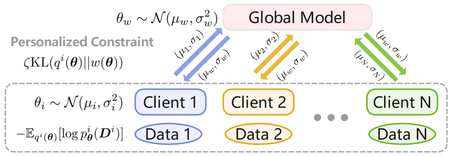
Figure 1: System diagram of the personalized Bayesian federated learning model under Gaussian assumptions.

2 Problem Formulation

In this section, we provide the problem formulation for Bayesian Federated Learning. Consider a distributed system in Fig. 1. There are $N$ clients and one server, where each client owns its personalized BNN. In each round, each client updates its personal distribution based on its data and the global distribution received from the server and then sends them to the server. The server aggregates the received local distribution parameters and then sends them to the clients. The $i$-th client has a dataset $\bm{D}^{i}=(\bm{D}_{1}^{i},\ldots,\bm{D}_{n}^{i})$ with $\bm{D}_{j}^{i}=(\bm{x}_{j}^{i},\bm{y}_{j}^{i}),i=1,\ldots,N$. The data follow the model

$$\bm{y}_{j}^{i}=f^{i}(\bm{x}_{j}^{i})+\varepsilon_{j}^{i},\,j=1,\ldots,n,\,\varepsilon_{j}^{i}\sim\mathcal{N}(0,\sigma_{\varepsilon}^{2}),$$ (1)

where $\bm{x}_{j}^{i}\in\mathbb{R}^{r_{0}}$, $\bm{y}_{j}^{i}\in\mathbb{R}^{r_{L+1}}$ for $j=1,\ldots,n$, $i=1,\ldots,N$, $f^{i}(\cdot):\mathbb{R}^{r_{0}}\to\mathbb{R}^{r_{L+1}}$ represents an unknown nonlinear function to be approximated, $n$ represents the number of samples, and $\sigma_{\varepsilon}$ represents the variance of noise. Our purpose is to propose a PFL model to approximate the unknown functions $\{f_{i}\}_{i=1}^{N}$ in the presence of heterogeneous and limited data.

Motivated by the universal approximation theorem [33], we use the fully-connected deep neural network (DNN) to approximate the unknown functions $\{f_{i}\}_{i=1}^{N}$ and represent the DNN model for the $i$-th client with $f_{\bm{\theta}}^{i}$. For the ease of aggregation of the server, we assume that all clients and the server share the same DNN structure but have different network parameters. Let the common neural network have $L$ hidden layers and the number of neurons for each layer be $r_{j},j=1,\ldots,L$, respectively. The DNN model is presented as

$$f_{\bm{\theta}}(\bm{x})=\bm{W}_{L+1}\sigma(\bm{W}_{L}\sigma(\ldots\sigma(\bm{W}_{1}\bm{x}+\bm{b}_{1}))+\bm{b}_{L})+\bm{b}_{L+1},$$ (2)

where $\sigma(\cdot)$ represents the activation function, $\bm{x}\in\mathbb{R}^{r_{0}}$, $\bm{W}_{j}\in\mathbb{R}^{r_{j-1}\times r_{j}}$ and $\bm{b}_{j}\in\mathbb{R}^{r_{j}}$. In this case, $\bm{\theta}\in\mathbb{R}^{T}$ represents the vector that stacks all weights $\{\bm{W}_{j}\}_{j=1}^{L+1}$ and biases $\{\bm{b}_{j}\}_{j=1}^{L+1}$. The length of $\bm{\theta}$ is denoted by $T=|\bm{\theta}|$. Define $\bm{r}=\{r_{1},\ldots,r_{L}\}$. Suppose that all the entries in $\bm{\theta}$ are bounded, i.e., $\left\lVert\bm{\theta}\right\rVert_{\infty}\leq B$, where $B>0$ stands for an absolute constant.

Next, we establish a bilevel optimization problem to estimate the distribution of the network parameters $\{\bm{\theta}_{i}\}_{i=1}^{N}$. To have a better understanding of the proposed model, we review the standard Bayesian variational inference in a single system [34, 35]. Let $\pi(\bm{\theta}|\bm{D})$ be the posterior distribution over data $\bm{D}$ and $q(\bm{\theta})\in\mathcal{Q}$ be the probability distribution to be learned. Variational inference (VI) seeks to learn the optimal distribution $q(\bm{\theta})$ that is closest to the posterior distribution $\pi(\bm{\theta}|\bm{D})$ in terms of KL divergence

$$\min_{q(\bm{\theta})\in\mathcal{Q}}\mbox{KL}\big{(}q(\bm{\theta})||\pi(\bm{\theta}|\bm{D})\big{)}.$$ (3)

By applying Bayes theorem $\pi(\bm{\theta}|\bm{D})\propto\pi(\bm{\theta})p_{\bm{\theta}}(\bm{D})$, the optimization problem (3) is reformulated to

$$\min_{q(\bm{\theta})\in\mathcal{Q}}-\mathbb{E}_{q(\bm{\theta})}[\log p_{\bm{\theta}}(\bm{D})]+\mbox{KL}(q(\bm{\theta})||\pi(\bm{\theta})),$$ (4)

where $\pi(\bm{\theta})$ stands for the prior distribution and $p_{\bm{\theta}}(\bm{D})$ stands for the likelihood. Here, the former term $-\mathbb{E}_{q(\bm{\theta})}[\log p_{\bm{\theta}}(\bm{D})]$ represents the reconstruction error over the data $\bm{D}$ while the latter term serves as a regularization term with the prior distribution. One disadvantage of vanilla VI is that it is difficult to characterize a good prior distribution of the dataset, but the performance of VI is dependent on a good choice of the prior distribution.

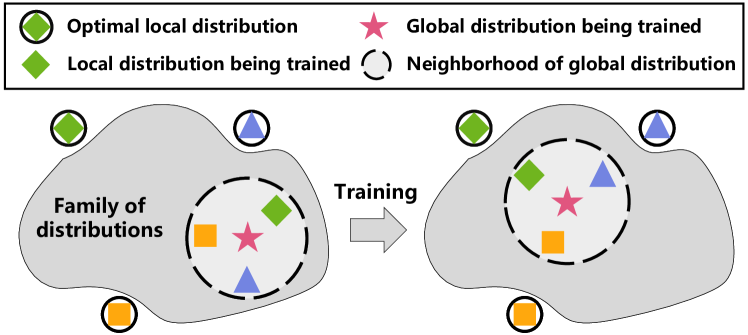
Figure 2: Distribution training of the personalized Bayesian federated learning model.

To avoid the disadvantage in the centralized setting, we use the global distribution from the server as a surrogate of the prior distribution in the distributed setting. Let $w(\bm{\theta})\in\mathcal{Q}_{w}$ be the probability distribution of the server’s network parameters and $q^{i}(\bm{\theta})\in\mathcal{Q}^{i}$ be the probability distribution of the $i$-th client’s network parameters, where $\mathcal{Q}_{w}$ and $\mathcal{Q}^{i}$ represent the family of distributions for the server and the $i$-th client, respectively. Based on the vanilla VI (4), we propose a new personalized Bayesian federated learning model by solving the following bilevel optimization problem

Server: $$~{}\min_{w(\bm{\theta})\in\mathcal{Q}_{w}}\left\{F(w)\triangleq\frac{1}{N}\sum_{i=1}^{N}F_{i}(w)\right\},$$ (5)

$$\text{Clients:}~{}F_{i}(w)\triangleq\min_{q^{i}(\bm{\theta})\in\mathcal{Q}^{i}}\Big{\{} -\mathbb{E}_{q^{i}(\bm{\theta})}[\log p^{i}_{\bm{\theta}}(\bm{D}^{i})]$$

$$+\zeta\,\mbox{KL}(q^{i}(\bm{\theta})||w(\bm{\theta}))\Big{\}}.$$ (6)

where $p^{i}_{\bm{\theta}}(\bm{D}^{i})$ represents the likelihood for the $i$-th client and $\zeta\geq 1$ is a constant that balances the personalization and global aggregation. The distribution training of the proposed model is shown in Fig. 2, which presents the change of the local and global distributions in probability space after training. The server aims to minimize its KL divergence with all the clients’ distributions, whereas each client seeks to strike a balance between minimizing the reconstruction error and minimizing the KL divergence with the global distribution.

3 Personalized Bayesian Federated Learning with Gaussian Distribution

In this section, we study the theory and algorithm of personalized Bayesian federated learning under Gaussian distribution. All elements of the network parameters are assumed to be independent and identically distributed (i.i.d.) Gaussian variables, which is a common assumption in the literature [36, 10, 11]. Specifically, we suppose that each entry of the server’s parameter vector $\bm{\theta}_{w}$ satisfies

$$\theta_{w,m}\sim\mathcal{N}(\mu_{w,m},\sigma^{2}_{w,m}),~{}m=1,\ldots,T,$$ (7)

where $\mu_{w,m}$ represents the mean and $\sigma_{w,m}$ represents the standard deviation of the $m$-th entry of the server. And suppose that each entry of the $i$-th client’s parameter vector $\bm{\theta}_{i}$ follows

$$\theta_{i,m}\sim\mathcal{N}(\mu_{i,m},\sigma^{2}_{i,m}),~{}m=1,\ldots,T,$$ (8)

where $\mu_{i,m}$ represents the mean and $\sigma_{i,m}$ represents the standard deviation of the $m$-th entry of the $i$-th client.

Based on the above assumptions, we can give a closed-form result for the KL divergences of $q^{i}(\bm{\theta})$ and $w(\bm{\theta})$, which is very useful in the following analysis and algorithm

$$~{}\mbox{KL}(q^{i}(\bm{\theta})||w(\bm{\theta}))$$

$$= ~{}\mbox{KL}\left(\prod^{T}_{m=1}\mathcal{N}(\mu_{i,m},\sigma^{2}_{i,m})\Bigl{|}\Bigr{|}\prod^{T}_{m=1}\mathcal{N}(\mu_{w,m},\sigma^{2}_{w,m})\right)$$

$$= ~{}\sum_{m=1}^{T}\mbox{KL}(\mathcal{N}(\mu_{i,m},\sigma^{2}_{i,m})||\mathcal{N}(\mu_{w,m},\sigma^{2}_{w,m}))$$ (9)

$$= ~{}\frac{1}{2}\sum_{m=1}^{T}\left[\log\left(\frac{\sigma_{w,m}^{2}}{\sigma_{i,m}^{2}}\right)+\frac{\sigma_{i,m}^{2}+(\mu_{i,m}-\mu_{w,m})^{2}}{\sigma_{w,m}^{2}}-1\right].$$

3.1 Theoretical Analysis

This subsection gives the theoretical guarantee for pFedBayes by analyzing the average generalization error bound, which presents that pFedBayes achieves the minimax error rate. The related proofs are delayed in the Appendices.

First of all, we provide some useful assumptions. The widths of all layers in BNNs are set to be the same [37, 38] and the activation function of each layer is set to be $1$-Lipschitz continuous.

Assumption 1.

The widths of all layers in BNNs are equal, i.e., $r_{i}=M,~{}i=1,\ldots,L$.

Assumption 2.

The activation function in BNNs is $1$-Lipschitz continuous, i.e., $\left\lVert\sigma(x)-\sigma(y)\right\rVert_{2}\leq\left\lVert x-y\right\rVert_{2}$.

Since each element in $\{\bm{\theta_{i}}\}_{i=1}^{N}$ is upper bounded by $B$, its variance is upper bounded by $B^{2}$, which is used in the proof of Lemma 2.

Assumption 3.

The parameters $r_{0},n,M,L$ are chosen suitably large such that

$$\sigma^{2}_{n}=\frac{T}{8n}A\leq B^{2},$$ (10)

where $H=BM$ and

$$A=\log^{-1}(3r_{0}M)\cdot(2H)^{-2(L+1)}$$

$$\left[\left(r_{0}+1+\frac{1}{H-1}\right)^{2}+\frac{1}{(2H)^{2}-1}+\frac{2}{(2H-1)^{2}}\right]^{-1}.$$ (11)

Next, we define the Hellinger distance

$$d^{2}(P_{\bm{\theta}}^{i},P^{i})=\mathbb{E}_{X}\Bigl{(}1-\exp\{-[f_{\bm{\theta}}^{i}(X)-f^{i}(X)]^{2}/(8\sigma^{2}_{\epsilon})\}\Bigr{)}$$ (12)

and

$$\chi_{n} =((L+1)T/n)\log M+(T/n)\log(r_{0}\sqrt{n/T}),$$ (13)

$$\xi^{i}_{n} =\inf_{\bm{\theta}\in{\Theta}(L,\bm{r}),\|\bm{\theta}\|_{\infty}\leq B}||f_{\bm{\theta}}^{i}-f^{i}||^{2}_{\infty},$$ (14)

$$\varepsilon_{n} =n^{-\frac{1}{2}}\sqrt{(L+1)T\log M+T\log(r_{0}\sqrt{n/T})}\log^{\delta}(n),$$ (15)

where $\delta>1$.

In order to give an upper bound of the average generalization error, we incorporate a constant in the bilevel optimization problem and the problem of the clients is reformulated as

$$\text{Clients:}~{}F_{i}(w)\triangleq\min_{q^{i}(\bm{\theta})\in\mathcal{Q}^{i}} \Big{\{}\int_{\Theta}l_{n}(P^{i},P^{i}_{\bm{\theta}})q^{i}(\bm{\theta})d\bm{\theta}$$

$$+\zeta\,\mbox{KL}(q^{i}(\bm{\theta})||w(\bm{\theta}))\Big{\}},$$ (16)

where $l_{n}(P^{i},P^{i}_{\bm{\theta}})$ is the log-likelihood ratio of $P^{i}$ and $P^{i}_{\bm{\theta}}$

$$l_{n}(P^{i},P^{i}_{\bm{\theta}})=\log\frac{p^{i}(\bm{D}^{i})}{p^{i}_{\bm{\theta}}(\bm{D}^{i})}.$$ (17)

Define $w^{\star}(\bm{\theta})$ as the solution of the server’s problem (5) and $\hat{q}^{i}(\bm{\theta})$ as the solution for the $i$-th client’s problem

$$w^{\star}(\bm{\theta})=\arg\min_{w(\bm{\theta})\in\mathcal{Q}_{w}}\left\{F(w)\triangleq\frac{1}{N}\sum_{i=1}^{N}F_{i}(w)\right\},$$ (18)

$$\hat{q}^{i}(\bm{\theta})=\arg\min_{q^{i}(\bm{\theta})\in\mathcal{Q}^{i}}\Big{\{} \int_{\Theta}l_{n}(P^{i},P^{i}_{\bm{\theta}})q^{i}(\bm{\theta})d\bm{\theta}$$

$$+\zeta\,\mbox{KL}(q^{i}(\bm{\theta})||w^{\star}(\bm{\theta}))\Big{\}}.$$ (19)

Next, we will provide an upper bound for the average generalization error

$$\frac{1}{N}\sum_{i=1}^{N}\int_{\Theta}d^{2}(P_{\bm{\theta}}^{i},P^{i})\hat{q}^{i}(\bm{\theta})d\bm{\theta}.$$ (20)

with the defined parameters $\chi_{n}$, $\xi^{i}_{n}$ and $\varepsilon_{n}$. The analysis is divided into two steps: we first give the bound with the average of (3.1) in Lemma 1 and then provide the upper bound of the average of (3.1) by using the optimality of $\hat{q}^{i}(\bm{\theta})$ in Lemma 2.

Lemma 1.

If Assumptions 1 and 2 hold, then the following inequality is satisfied with dominating probability

$$\frac{1}{N} \sum_{i=1}^{N}\int_{\Theta}d^{2}(P_{\bm{\theta}}^{i},P^{i})\hat{q}^{i}(\bm{\theta})d\bm{\theta}\leq$$

$$\frac{1}{n}\Bigg{\{}\frac{1}{N}\sum_{i=1}^{N}\Bigg{[}\frac{1}{\zeta}\int_{\Theta}l_{n}(P^{i},P^{i}_{\bm{\theta}})\hat{q}^{i}(\bm{\theta})d\bm{\theta}$$

$$\qquad\qquad\quad+\mbox{\rm KL}(\hat{q}^{i}(\bm{\theta})||w^{\star}(\bm{\theta}))\Bigg{]}\Bigg{\}}+C\varepsilon^{2}_{n},$$ (21)

where $\zeta\geq 1$ is a balance parameter and $C>0$ is a constant.

Lemma 2.

If Assumptions 1-3 hold, then the following inequality is satisfied with dominating probability

$$\frac{1}{N}\sum_{i=1}^{N}\left[\int_{\Theta}l_{n}(P^{i},P^{i}_{\bm{\theta}})\hat{q}^{i}(\bm{\theta})d\bm{\theta}+\zeta\,\mbox{\rm KL}(\hat{q}^{i}(\bm{\theta})||w^{\star}(\bm{\theta}))\right]\\ \leq n\left(C^{\prime}\zeta\chi_{n}+\frac{C^{\prime\prime}}{N}\sum_{i=1}^{N}\xi^{i}_{n}\right),$$ (22)

where $\zeta\geq 1$ is a balance parameter and $C^{\prime},C^{\prime\prime}$ are arbitrary diverging sequences.

By combining Lemmas 1 and 2, we obtain the generalization error bound as follows.

Theorem 1.

If Assumptions 1-3 hold, then the following generalization error upper bound is satisfied with dominating probability

$$\frac{1}{N}\sum_{i=1}^{N}\int_{\Theta}d^{2}(P_{\bm{\theta}}^{i},P^{i})\hat{q}^{i}(\bm{\theta})d\bm{\theta}\\ \leq C\varepsilon^{2}_{n}+C^{\prime}\chi_{n}+\frac{C^{\prime\prime}}{N\zeta}\sum_{i=1}^{N}\xi^{i}_{n},$$ (23)

where $\zeta\geq 1$ is a balance parameter, $C>0$ is a constant and $C^{\prime},C^{\prime\prime}$ are arbitrary diverging sequences.

Remark 1.

From (23), we see that the upper bound and the approximation error decrease as $\zeta$ increases. However, the degree of customisation decreases as $\zeta$ increases, which is not what we want. Therefore, we should choose a suitable parameter $\zeta$ such that the degree of customisation and the average generalization error bound can be balanced.

As for Theorem 1, the upper bound is divided into two kinds of error: the sum of the first two terms is the estimation error and the third term is the approximation error. According to the definitions of $\chi_{n}$ and $\varepsilon_{n}$, we obtain that the error bound gets smaller as the sample size $n$ increases and gets bigger as $T$ increases. However, the approximation error decreases with the increase of $T$ (or the width and depth). In order to balance the upper bound, we should choose a suitable $T$ as a function of the number of samples $n$.

Next, we discuss how to choose $T$ for $\beta$-Hölder-smooth functions $\{f^{i}\}$. Let the intrinsic dimension of data be $d$. From [39, Corollary 6], the approximation error $\{\xi^{i}_{n}\}_{i=1}^{N}$ is upper bounded

$$\xi^{i}_{n}\leq C_{0}T^{-2\beta/d},i=1,\ldots,N,$$ (24)

where $C_{0}>0$ represents a constant related to $r_{0}$, $\beta$ and $d$. By choosing $T=C_{1}n^{d/(2\beta+d)}$ in Theorem 1, the generalization bound is given by

$$\frac{1}{N}\sum_{i=1}^{N}\int_{\Theta}d^{2}(P_{\bm{\theta}}^{i},P^{i})\hat{q}^{i}(\bm{\theta})d\bm{\theta}\leq C_{2}n^{-\frac{2\beta}{2\beta+d}}\log^{2\delta^{\prime}}(n),$$ (25)

where $C_{1},C_{2}>0$ are constants related to $r_{0}$, $\beta$, $d$, $L$, $M$, $\zeta$ and $n$ and $\delta^{\prime}>\delta>1$.

In the end, we demonstrate that the proposed pFedBayes achieves minimax optimality of the generalization error rate. Like [38, Theorem 1.1], we can restate the upper bound using $L^{2}$ norm. Since the function $[1-\exp(-x^{2})]/{x^{2}}$ is monotonically decreasing for $x>0$, for bounded functions $\left\lVert f^{i}\right\rVert_{\infty}\leq F$, $i=1,\ldots,N$, the following inequality holds

$$\frac{d^{2}(P_{\bm{\theta}}^{i},P^{i})}{\left\lVert f_{\bm{\theta}}^{i}(X)-f^{i}(X)\right\rVert_{L^{2}}^{2}}\geq\frac{1-\exp(-\frac{4F^{2}}{8\sigma_{\epsilon}^{2}})}{4F^{2}}\triangleq C_{F}.$$ (26)

Combining with (25), we provide the upper bound of the generalization error using $L^{2}$ norm

$$\frac{C_{F}}{N}\sum_{i=1}^{N}\int_{\Theta}\left\lVert f_{\bm{\theta}}^{i}(X^{i})-f^{i}(X^{i})\right\rVert_{L^{2}}^{2}\hat{q}^{i}(\bm{\theta})d\bm{\theta}\\ \leq\frac{1}{N}\sum_{i=1}^{N}\int_{\Theta}d^{2}(P_{\bm{\theta}}^{i},P^{i})\hat{q}^{i}(\bm{\theta})d\bm{\theta}\\ \leq C_{2}n^{-\frac{2\beta}{2\beta+d}}\log^{2\delta^{\prime}}(n).$$ (27)

Together with the minimax lower bound using $L^{2}$ norm in [39, Theorem 8], we have

$$\inf_{\{\left\lVert f_{\bm{\theta}}^{i}\right\rVert\leq F\}_{i=1}^{N}}\sup_{\{\left\lVert f^{i}\right\rVert_{\infty}\leq F\}_{i=1}^{N}}\frac{C_{F}}{N}\sum_{i=1}^{N}\\ \int_{\Theta}\left\lVert f_{\bm{\theta}}^{i}(X^{i})-f^{i}(X^{i})\right\rVert_{L^{2}}^{2}\hat{q}^{i}(\bm{\theta})d\bm{\theta}\geq C_{3}n^{-\frac{2\beta}{2\beta+d}},$$ (28)

where $C_{3}>0$ is a constant.

Since the minimax lower bound (28) matches the upper bound (27), we come to a conclusion that the convergence rate of the average generalization error of pFedBayes is minimax optimal up to a logarithmic term for bounded functions $\{f^{i}\}_{i=1}^{N}$ and $\{f^{i}_{\bm{\theta}}\}_{i=1}^{N}$.

Algorithm 1 pFedBayes: Personalized Bayesian Federated Learning Algorithm

Server executes:

Input $T,R,S,\beta,a,b,\bm{v}^{0}=(\bm{\mu}^{0},\bm{\rho}^{0})$

for $t=0,1,...,T-1$ do

for $i=1,2,...,N$ in parallel do

$\bm{v}_{i}^{t+1}\leftarrow\text{ClientUpdate}(i,\bm{v}^{t})$

$\mathbb{S}^{t}\leftarrow\text{Random index sets of $S$ clients}$

$\bm{v}^{t+1}=(1-\beta)\bm{v}^{t}+\frac{\beta}{S}\sum_{i\in\mathbb{S}^{t}}{\bm{v}_{i}^{t+1}}$

$\textbf{ClientUpdate}(i,\bm{v}^{t})\textbf{:}$

$\bm{v}_{w,0}^{t}=\bm{v}^{t}$

for $r=0,1,...,R-1$ do

$\bm{D}^{i}_{\Lambda}$ $\leftarrow$ Minibatch sampling with size $b$ from $\bm{D}^{i}$

$\bm{g}_{i,r}$ $\leftarrow$ Random sampling with size $a$ from $\mathcal{N}(0,1)$

$\Omega^{i}(\bm{v}_{r}^{t})$ $\leftarrow$ Apply (30) with $\bm{g}_{i,r}$, $\bm{D}^{i}_{\Lambda}$ and $\bm{v}_{r}^{t}$

$\bm{v}_{r}^{t}$ $\leftarrow$ Update with $\nabla\Omega(\bm{v}_{r}^{t})$ via GD algorithms

$\bm{v}_{w,r+1}^{t}$ $\leftarrow$ Update with $\nabla\Omega(\bm{v}_{w,r}^{t})$ via GD algorithms

return $\bm{v}_{w,R}^{t}$ to the server

3.2 Algorithm

This subsection presents the implementation of pFedBayes using the stochastic gradient descent (SGD) algorithms, which is shown in Algorithm 1. In order to represent the distribution of the network parameter $\bm{\theta}$, we introduce two new parameters $\bm{\mu}$ and $\bm{\rho}$, where $\mu_{m}$ represents the mean and $\sigma_{m}=\log(1+\exp(\rho_{m}))$ represents the standard deviation of the random variable ${\theta}_{m}$. The reason we use $\rho_{m}$ instead of $\sigma_{m}$ is to make $\sigma_{m}$ non-negative. Define the parameter tuple $\bm{v}=(\bm{\mu},\bm{\rho})$. We can reformulate the vector $\bm{\theta}$ as $\bm{\theta}=h({\bm{v}},\bm{g})$, where

$$\theta_{m}=h({v_{m}},g_{m})=\mu_{m}+\log(1+\exp(\rho_{m}))\cdot g_{m},~{}~{}g_{m}\sim\mathcal{N}(0,1).$$ (29)

Then we rewrite the distribution of $\bm{\theta}$ as $q_{\bm{v}}(\bm{\theta})$, where $q_{\bm{v}}(\theta_{m})=\mathcal{N}\big{(}\mu_{m},\log^{2}(1+\exp(\rho_{m}))\big{)},m=1,\ldots,T$.

To reduce the cost of communication, we update a localized global model and the local model for $R$ rounds alternatively on the clients’ side and then aggregate the localized global models in the server. We start with approximating the objective function of local clients in (2). Under Gaussian assumptions, the KL divergence term can be calculated by using (3). But we cannot obtain a closed-form result for the first term in (2). Instead, Monte Carlo approximation is applied to estimation the first term. To accelerate the convergence, we utilize a minibatch of the samples in the approximation. Particularly, the objective function for the $i$-th client is represented as

$$\Omega^{i}(\bm{v})\approx-\frac{n}{b}\frac{1}{a}\sum_{j=1}^{b}\sum_{k=1}^{a}\log p^{i}_{h({\bm{v}},\bm{g}_{k})}(\bm{D}^{i}_{j})\\ +\zeta\,\mbox{KL}(q^{i}_{\bm{v}}(\bm{\theta})||w_{\bm{v}}(\bm{\theta})),$$ (30)

where $b$ and $a$ are minibatch size and Monte Carlo sample size, respectively. The corresponding objective function of the $i$-th localized global model is given by

$$\Omega^{i}_{w}(\bm{v})=\mbox{KL}(q^{i}_{\bm{v}}(\bm{\theta})||w_{\bm{v}}(\bm{\theta})).$$ (31)

The clients make $R$ iterations and send the updated localized global models to the server. At each iteration of the clients, the algorithm updates the personalized models with $\nabla_{\bm{v}}\Omega^{i}(\bm{v})$ and the localized global models with $\nabla_{\bm{v}}\Omega^{i}_{w}(\bm{v})$ alternatively. Considering the silence of some clients in practice, we assume that only a random subset of the clients upload their parameters. The subset is defined as $\mathbb{S}^{t}\in\{1,\ldots,N\}$ and its size is $S$. After receiving the parameters of the clients in $\mathbb{S}^{t}$, the server takes the mean of the clients and makes an extrapolation step to speed up the algorithm. The parameter for the extrapolation step is defined as $\beta$.

4 Sparse Personalized Federated Learning with Bernoulli-Gaussian distribution

In this section, we consider the algorithm of sparse personalized federated learning. To promote a sparse DNN structure, we use a spike-and-slab prior on each component of $\bm{\theta}$ [40, 38]. In particular, we use Bernoulli-Gaussian distribution as the prior distribution.

Suppose that each entry of the $i$-th client $\mathcal{Q}^{i}$ follows

$$\theta_{i,m}|\gamma_{i,m}\sim\gamma_{i,m}\mathcal{N}(\mu_{i,m},\sigma^{2}_{i,m})+(1-\gamma_{i,m})\delta_{0},\\ \gamma_{i,m}\sim\mbox{Bern}(\lambda_{i,m}),\,m=1,\ldots,T,$$ (32)

where $\lambda_{i,m}$ represents the inclusion probability, $\mu_{i,m}$ represents the mean and $\sigma^{2}_{i,m}$ represents the variance of a Gaussian distribution for $m$-th entry of the $i$-th client and $\delta_{0}$ represents the Dirac at $0$. Suppose that each entry of the server satisfies

$$\theta_{w,m}|\gamma_{w,m}\sim\gamma_{w,m}\mathcal{N}(\mu_{w,m},\sigma^{2}_{w,m})+(1-\gamma_{w,m})\delta_{0},\\ \gamma_{w,m}\sim\mbox{Bern}(\lambda_{w,m}),\,m=1,\ldots,T,$$ (33)

where $\lambda_{w,m}$ represents the inclusion probability, $\mu_{w,m}$ represents the mean and $\sigma^{2}_{w,m}$ represents the variance of a Gaussian distribution for $m$-th entry of the server.

Under the above distribution assumptions (32) and (33), we can give the upper bound of KL divergence for the two Bernoulli-Gaussian distributions

$$\mbox{KL}(q^{i}(\theta)||w(\theta)))$$

$$\leq\sum_{m=1}^{T}\mbox{KL}(q^{i}(\gamma_{m})||w(\gamma_{m}))$$

$$+\sum_{m=1}^{T}q^{i}(\gamma_{m}=1)\mbox{KL}(\mathcal{N}(\mu_{i,m},\sigma^{2}_{i,m})||\mathcal{N}(\mu_{w,m},\sigma^{2}_{w,m}))$$

$$=\sum_{m=1}^{T}\left[\lambda_{i,m}\log\left(\frac{\lambda_{i,m}}{\lambda_{w,m}}\right)+(1-\lambda_{i,m})\log\left(\frac{1-\lambda_{i,m}}{1-\lambda_{w,m}}\right)\right]$$

$$+\sum_{m=1}^{T}\frac{\lambda_{i,m}}{2}\left[\log\left(\frac{\sigma_{w,m}^{2}}{\sigma_{i,m}^{2}}\right)+\frac{\sigma_{i,m}^{2}+(\mu_{i,m}-\mu_{w,m})^{2}}{\sigma_{w,m}^{2}}-1\right],$$ (34)

where $q^{i}(\gamma_{m})=\lambda_{i,m}^{\gamma_{m}}(1-\lambda_{i,m})^{(1-\gamma_{m})}$, and $w(\gamma_{m})=\lambda_{w,m}^{\gamma_{m}}(1-\lambda_{w,m})^{(1-\gamma_{m})}$.

4.1 Theretical analysis

The generalization error bound for the sparse case can be obtained by simply replacing the total number of parameters $T$ with an optimal sparsity $s^{\star}_{i}$ of each neural network [40], which is omitted for brevity.

Before giving the results, we define some parameters and give some assumptions. Let $B>0$ be an absolute constant such that $|\theta_{i,m}|,|\theta_{w,m}|\leq B$, and define

$$\bar{\chi}^{i}_{n}\triangleq\big{(}(L+1)s^{\star}_{i}/{n}\big{)}\log M+({s^{\star}_{i}}/{n})\log\big{(}r_{0}\sqrt{{n}/{s^{\star}_{i}}}\big{)},$$ (35)

$$\bar{\xi}^{i}_{n}\triangleq\inf_{\bm{\theta}\in\Theta(L,\bm{r},s^{\star}),\|\bm{\theta}\|_{\infty}\leq B}||f_{\theta}^{i}-f^{i}||^{2}_{\infty},$$ (36)

$$\bar{\varepsilon}^{i}_{n}\triangleq\sqrt{\bar{\chi}^{i}_{n}}\log^{\delta}(n).$$ (37)

Assumption 4.

For the $i$-th cilent, the hyperparameter $\sigma_{i}^{2}>0$ is an absolute constant, and $\lambda_{i}$ satisfies $\log(1/\lambda_{i})=O\{(L+1)\log M+\log(r_{0}\sqrt{n/s^{\star}_{i}})\}$ and $\log(1/(1-\lambda_{i}))=O((s^{\star}_{i}/T)\{(L+1)\log M+\log(r_{0}\sqrt{n/s^{\star}_{i}})\})$.

Assumption 5.

The parameters $r_{0},n,M,L$ is large enough such that

$$\sigma_{i,n}^{2}=\frac{s^{\star}_{i}}{8n}A\leq B^{2}.$$ (38)

where $A$ is defined in Eq. (3).

Theorem 2.

If Assumptions 1,2, 4 and 5 are true, then the following generalization error upper bound is satisfied with dominating probability

$$\frac{1}{N}\sum_{i=1}^{N}\int_{\Theta}d^{2}(P_{\bm{\theta}}^{i},P^{i})\hat{q}^{i}(\bm{\theta})d\bm{\theta}\\ \leq\frac{1}{N}\sum_{i=1}^{N}\Big{[}C[\bar{\varepsilon}^{i}_{n}]^{2}+C^{\prime}\bar{\chi}_{n}^{i}+\frac{C^{\prime\prime}}{\zeta}\bar{\xi}^{i}_{n}\Big{]},$$ (39)

where $\zeta\geq 1$ is a balance parameter, $C>0$ is a constants and $C^{\prime},C^{\prime\prime}$ are arbitrary diverging sequences.

A well-chosen sparsity can strike a balance between estimation error and approximation error. Combining with approximation error from [41], it can be shown that the upper bound is minimax rate optimal up to a logarithmic term for the sparse personalized federated learning model.

4.2 Algorithm

In order to implement the proposed model, we reparameterize $\bm{\theta}$ with a tuple $\bm{v}=(\bm{\mu},\bm{\rho},\bm{\lambda})$. After reparameterization, we obtain $\bm{\theta}=\phi(\bm{v},\bm{\gamma},\bm{g})$, where

$$\theta_{m}=\phi(v_{m},\gamma_{m},g_{m})=\gamma_{m}[\mu_{m}+\log(1+\exp(\rho_{m}))\cdot g_{m}],\\ ~{}~{}\gamma_{m}\sim\mbox{Bern}(\lambda_{m}),~{}g_{m}\sim\mathcal{N}(0,1).$$ (40)

Since the discrete distribution of Bernoulli makes it difficult to backpropagate the gradient with respect to $\gamma$, we only use the Bernoulli variable in the forward pass and approximate it by a continuous function in the backward pass. Motivated by the work [38], we use the Gumbel-softmax approximation here. Particularly, we use $\tilde{\gamma}\sim\mbox{Gumbel-softmax}(\lambda,\tau)$ to approach $\gamma\sim\mbox{Bern}(\lambda)$, where

$$\widetilde{\gamma}=(1+\exp(-\eta/\tau))^{-1},\\ \eta=\log\frac{\lambda}{1-\lambda}+\log\frac{u}{1-u},\quad u\sim\mathcal{U}(0,1).$$ (41)

Define the localized global model of the $i$-th client

$$\Omega^{i}_{w}(\bm{v})=$$

$$\sum_{m=1}^{T}\left[\lambda_{i,m}\log\left(\frac{\lambda_{i,m}}{\lambda_{w,m}}\right)+(1-\lambda_{i,m})\log\left(\frac{1-\lambda_{i,m}}{1-\lambda_{w,m}}\right)\right]$$

$$+\sum_{m=1}^{T}\frac{\lambda_{i,m}}{2}\left[\log\left(\frac{\sigma_{w,m}^{2}}{\sigma_{i,m}^{2}}\right)+\frac{\sigma_{i,m}^{2}+(\mu_{i,m}-\mu_{w,m})^{2}}{\sigma_{w,m}^{2}}-1\right].$$ (42)

For the local model of the $i$-th client, we use the Monte Carlo estimation to approximate the local loss. In particular, the stochastic estimator for the $i$-th client is given by

$$\Omega^{i}(\bm{v})\approx-\frac{n}{b}\frac{1}{a}\sum_{j=1}^{b}\sum_{k=1}^{a}\log p^{i}_{\phi(\bm{v},{\bm{\gamma}}_{k},{\bm{g}}_{k})}(D^{i}_{j})+\zeta\,\Omega^{i}_{w}(\bm{v}),$$ (43)

where $b$ and $a$ are minibatch size and Monte Carlo sample size, respectively. So we can give the algorithm in Algorithm 2.

Algorithm 2 sFedBayes: Sparse Personalized Bayesian Federated Learning Algorithm

Server executes:

Input $T,R,S,\tau,\eta,a,b,\beta,\bm{v}^{0}=(\bm{\mu}^{0},\bm{\rho}^{0},\bm{\lambda}^{0})$

for $t=0,1,...,T-1$ do

for $i=1,2,...,N$ in parallel do

$\bm{v}_{i}^{t+1}\leftarrow\text{ClientUpdate}(i,\bm{v}^{t})$

$\mathbb{S}^{t}\leftarrow\text{Random index sets of $S$ clients}$

$\bm{v}^{t+1}=(1-\beta)\bm{v}^{t}+\frac{\beta}{S}\sum_{i\in\mathbb{S}^{t}}{\bm{v}_{i}^{t+1}}$

$\textbf{ClientUpdate}(i,\bm{v}^{t})\textbf{:}$

$\bm{v}_{w,0}^{t}=\bm{v}_{0}^{t}=\bm{v}^{t}$

for $r=0,1,...,R-1$ do

$\mathcal{D}^{i}_{\Lambda}$ $\leftarrow$ Minibatch sampling with size $b$ from $\mathcal{D}^{i}$

$\epsilon_{i,r},u_{i,r}$ $\leftarrow$ Random sampling with size $a$ from $\mathcal{N}(0,1)$

and $\mathcal{U}(0,1)$

$\Omega^{i}(\bm{v}_{r}^{t})$ $\leftarrow$ Apply (43) with $\mathcal{D}^{i}_{\Lambda}$, $\epsilon_{i,r},u_{i,r}$ and $v_{r}^{t}$

$\bm{v}_{r}^{t}$ $\leftarrow$ Update with $\nabla\Omega(\bm{v}_{r}^{t})$ via GD algorithms

$\bm{v}_{w,r+1}^{t}$ $\leftarrow$ Update with $\nabla\Omega(\bm{v}_{w,r}^{t})$ via GD algorithms

return $\bm{\bm{v}}_{w,R}^{t}$ to the server

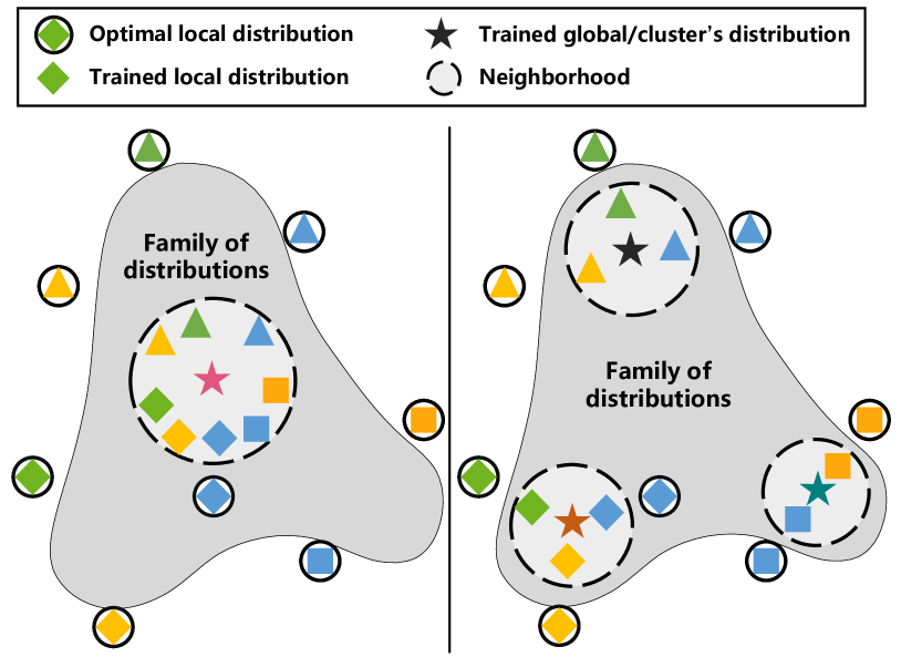
Figure 3: Comparisons for personalized Bayesian federated learning model and clustered Bayesian federated learning model. Left: Personalized Bayesian federated learning model; Right: Clustered Bayesian federated learning model. The clients with the same shape belong to the same cluster.

5 Clustered Federated Learning via Bayesian Inference

We propose a clustered Bayesian federated learning model in this section. When the data among clients are quite different, the global distribution obtained by pFedBayes cannot serve as the good prior distribution. To overcome the extreme heterogeneity from non-i.i.d. data, we consider learning multiple prior distributions to improve the personalization performance. As shown in Fig. 3, the prior distributions generated by clustered FL for different clusters are much better than that generated by vanilla personalized FL, implying that clustered FL can achieve better personalization than vanilla personalized FL.

Let $N$ be the number of clients, and $K$ be the number of clusters with $K<N$. We propose the following bilevel optimization method named cFedBayes to achieve clustered federated learning via Bayesian inference

$$\text{Server:}\min_{\{w^{k}(\bm{\theta})\}_{k=1}^{K}}\left\{\frac{1}{N}\sum_{i=1}^{N}F_{i}\big{(}\{w^{k}\}_{k=1}^{K}\big{)}\right\},$$ (44)

$$\text{Clients:}~{}\\ F_{i}\big{(}\{w^{k}\}_{k=1}^{K}\big{)}\triangleq\min_{q^{i}(\bm{\theta})\in\mathcal{Q}^{i},\tilde{k}^{i}}\Big{\{}-\mathbb{E}_{q^{i}(\bm{\theta})}[\log p^{i}(\bm{D}^{i}|{\bm{\theta}})]\\ +\zeta\mbox{KL}(q^{i}(\bm{\theta})||w^{\tilde{k}^{i}}(\bm{\theta}))\mid\tilde{k}^{i}=\arg\max_{k}\mathbb{E}_{w^{k}(\bm{\theta})}[\log p^{i}(\bm{D}^{i}|\bm{\theta})]\Big{\}},$$ (45)

where $w^{k}(\bm{\theta})$ is the parameter to be optimized for the $k$-th cluster, $q^{i}(\bm{\theta})$ is the parameter to be optimized for the $i$-th client and $\tilde{k}^{i}$ represents the the cluster of $i$-th client. Different from pFedBayes, the incorporation of clusters makes cFedBayes applicable for extreme heterogeneity from non-i.i.d. data.

5.1 Theoretical analysis

In order to give an upper bound of the average generalization error, we incorporate a constant in the bilevel optimization problem and the problem of the clients is reformulated as

$$F_{i}\big{(}\{w^{k}\}_{k=1}^{K}\big{)}=\min_{q^{i}(\bm{\theta})\in\mathcal{Q}^{i},\tilde{k}^{i}}\bigg{\{}\int_{\Theta}l_{n}(P^{i},P^{i}_{\bm{\theta}})q^{i}(\bm{\theta})d\bm{\theta}$$

$$+\zeta\mbox{KL}(q^{i}(\bm{\theta})||w^{\tilde{k}^{i}}(\bm{\theta}))\mid\tilde{k}^{i}=\underset{k}{\mbox{argmin}}\int_{\Theta}l_{n}(P^{i},P^{i}_{\bm{\theta}})w^{k}(\bm{\theta})d\bm{\theta}\bigg{\}},$$ (46)

where $l_{n}(P^{i},P^{i}_{\bm{\theta}})$ is defined in (17).

Let $\{\hat{w}^{k}(\bm{\theta})\}_{k=1}^{K}$ be solution of the problem (44) and $\hat{q}^{i}(\bm{\theta})$ and $\hat{k}^{i}$ be its corresponding solution for the $i$-th client’s subproblem

$$(\hat{q}^{i}(\bm{\theta}),\hat{k}^{i})=\arg\min_{q^{i}(\bm{\theta})\in\mathcal{Q}^{i},\tilde{k}^{i}}\bigg{\{}\int_{\Theta}l_{n}(P^{i},P^{i}_{\bm{\theta}})q^{i}(\bm{\theta})d\bm{\theta}$$

$$+\zeta\mbox{KL}(q^{i}(\bm{\theta})||\hat{w}^{\tilde{k}^{i}}(\bm{\theta}))\mid\tilde{k}^{i}=\underset{k}{\mbox{argmin}}\int_{\Theta}l_{n}(P^{i},P^{i}_{\bm{\theta}})\hat{w}^{k}(\bm{\theta})d\bm{\theta}\bigg{\}}.$$ (47)

Here, we suppose that only one cluster minimizes $\int_{\Theta}l_{n}(P^{i},P^{i}_{\bm{\theta}})\hat{w}^{k}(\bm{\theta})d\bm{\theta}$; otherwise, we can choose one index randomly that minimizes $\int_{\Theta}l_{n}(P^{i},P^{i}_{\bm{\theta}})\hat{w}^{k}(\bm{\theta})d\bm{\theta}$.

Let $\mathbb{S}_{k}=\{i|\hat{k}^{i}=k\}$ denote the index set of all clients that belong to the $k$-th cluster. Our goal is to give an upper bound for each cluster

$$\frac{1}{|\mathbb{S}_{k}|}\sum_{i\in\mathbb{S}_{k}}\int_{\Theta}d^{2}(P_{\bm{\theta}}^{i},P^{i})\hat{q}^{i}(\bm{\theta})d\bm{\theta},~{}k=1,\ldots,K.$$ (48)

with parameters $\chi_{n}$, $\xi^{i}_{n}$ and $\varepsilon_{n}$.

We first give the upper bound of $\int_{\Theta}d^{2}(P_{\bm{\theta}}^{i},P^{i})\hat{q}^{i}(\bm{\theta})d\bm{\theta}$ in Lemma 3 and then give the upper bound of the right-hand side of Lemma 3 in Lemma 4.

Lemma 3.

If Assumptions 1 and 2 hold, then the following inequality is satisfied with dominating probability

$$\int_{\Theta}d^{2}(P_{\bm{\theta}}^{i},P^{i})\hat{q}^{i}(\bm{\theta})d\bm{\theta}\leq\frac{1}{n}\Bigg{\{}\frac{1}{\zeta}\int_{\Theta}l_{n}(P^{i},P^{i}_{\bm{\theta}})\hat{q}^{i}(\bm{\theta})d\bm{\theta}\\ +\mbox{\rm KL}(\hat{q}^{i}(\bm{\theta})||\hat{w}^{\hat{k}^{i}}(\bm{\theta}))\Bigg{\}}+C\varepsilon^{2}_{n},$$ (49)

where $\zeta\geq 1$ is a balance parameter and $C>0$ is a constant.

Lemma 4.

If Assumptions 1-3 hold, then the following inequality is satisfied with dominating probability

$$\frac{1}{|\mathbb{S}_{k}|}\sum_{i\in\mathbb{S}_{k}}\Bigg{[}\int_{\Theta}l_{n}(P^{i},P^{i}_{\bm{\theta}})\hat{q}^{i}(\bm{\theta})d\bm{\theta}+\zeta\,\mbox{\rm KL}(\hat{q}^{i}(\bm{\theta})||\hat{w}^{\hat{k}^{i}}(\bm{\theta}))\Bigg{]}\\ \leq n\left(C^{\prime}\zeta\chi_{n}+\frac{C^{\prime\prime}}{|\mathbb{S}_{k}|}\sum_{i\in\mathbb{S}_{k}}\xi^{i}_{n}\right),$$ (50)

where $\zeta\geq 1$ is a balance parameter and $C^{\prime},C^{\prime\prime}$ are arbitrary diverging sequences.

By combining Lemmas 3 and 4, we obtain the generalization error bound for cFedBayes as follows.

Theorem 3.

If Assumptions 1-3 hold, then the following generalization error upper bound is satisfied with dominating probability

$$\frac{1}{|\mathbb{S}_{k}|}\sum_{i\in\mathbb{S}_{k}}\int_{\Theta}d^{2}(P_{\bm{\theta}}^{i},P^{i})\hat{q}^{i}(\bm{\theta})d\bm{\theta}\\ \leq C\varepsilon^{2}_{n}+C^{\prime}\chi_{n}+\frac{C^{\prime\prime}}{|\mathbb{S}_{k}|\zeta}\sum_{i\in\mathbb{S}_{k}}\xi^{i}_{n},$$ (51)

where $\zeta\geq 1$ is a balance parameter, $C>0$ is an constant and $C^{\prime},C^{\prime\prime}$ are arbitrary diverging sequences.

Suppose that the unknown functions $\{f^{i}\}_{i\in\mathbb{S}_{k}}$ are $\beta_{k}$-Hölder-smooth and all data has $d$ intrinsic dimension. In this case, the order of the generalization error rate for pFedBayes appears as

$$\frac{1}{N}\sum_{i=1}^{N}\int_{\Theta}d^{2}(P_{\bm{\theta}}^{i},P^{i})\hat{q}^{i}(\bm{\theta})d\bm{\theta}\\ =\mathcal{O}\left(\frac{1}{N}\sum_{k=1}^{K}|\mathbb{S}_{k}|n^{-\frac{2\beta_{k}}{2\beta_{k}+d}}\log^{2\delta^{\prime}}(n)\right)\\ =\mathcal{O}\left(n^{-\frac{2\beta}{2\beta+d}}\log^{2\delta^{\prime}}(n)\right),$$ (52)

where $\beta=\min\{\beta_{1},\ldots,\beta_{K}\}$. Following the discussions from the minimax optimality of pFedBayes, we conclude that the convergence rate of the generalization error of cFedBayes is minimax optimal up to a logarithmic term for bounded $\{f^{i}\}_{i\in\mathbb{S}_{k}}$ and $\{f^{i}_{\bm{\theta}}\}_{i\in\mathbb{S}_{k}}$. And the order of the generalization error rate for cFedBayes is

$$\frac{1}{|\mathbb{S}_{k}|}\sum_{i\in\mathbb{S}_{k}}\int_{\Theta}d^{2}(P_{\bm{\theta}}^{i},P^{i})\hat{q}^{i}(\bm{\theta})d\bm{\theta}=\mathcal{O}\left(n^{-\frac{2\beta_{k}}{2\beta_{k}+d}}\log^{2\delta^{\prime}}(n)\right)$$ (53)

for $k=1,\ldots,K$. Since $\beta_{k}\geq\beta$, comparing (53) with (52) implies that clustered federated learning has a tighter generalization error rate than personalized federated learning, which means that cFedBayes has better performance than pFedBayes.

5.2 Algorithm

This section describes how to integrate cFedBayes in a federated learning system. To reduce the communication cost, the global parameters are updated for a few rounds on the clients’ side and then aggregated on the server’s side.

Define $\bm{v}=(\bm{\mu},\bm{\rho})$. Then $\bm{\theta}$ can be reparameterized as $\bm{\theta}=h({\bm{v}},\bm{g})$, where

$$\theta_{m}=h({v_{m}},g_{m})=\mu_{m}+\log(1+\rho_{m})\cdot g_{m},~{}~{}g_{m}\sim\mathcal{N}(0,1).$$ (54)

For any $q\sim\{\mathcal{Q}^{i}\}_{i=1}^{N}\cup\mathcal{Q}^{w}$, the distribution of the random vector $\bm{\theta}$ is rewritten as $q_{\bm{v}}(\bm{\theta})$, where $q_{\bm{v}}(\theta_{m})=\mathcal{N}(\mu_{m},\rho_{m}^{2}),m=1,\ldots,T$.

The cost function for the $i$-th client is shown as

$$\Omega^{i}(\bm{v})\approx-\frac{n}{b}\frac{1}{a}\sum_{j=1}^{b}\sum_{l=1}^{a}\log p^{i}_{h({\bm{v}},\bm{g}_{l})}(\bm{D}^{i}_{j})\\ +\zeta\,\mbox{KL}(q^{i}_{\bm{v}}(\bm{\theta})||w^{\tilde{k}^{i}}_{\bm{v}}(\bm{\theta})),\bm{\theta}\sim q^{i}_{\bm{v}}$$ (55)

where

$$\tilde{k}^{i}=\underset{k}{\mbox{arg max}}\,\frac{n}{b}\frac{1}{a}\sum_{j=1}^{b}\sum_{l=1}^{a}\log p^{i}_{h({\bm{v}},\bm{g}_{l})}(\bm{D}^{i}_{j}),\bm{\theta}\sim w^{k}_{\bm{v}},$$ (56)

and $n$, $b$ and $a$ are sample size, minibatch size, and Monte Carlo sample size, respectively.

The objective function of the $i$-th localized global model is represented by

$$\Omega^{i}_{w}(\bm{v})=\mbox{KL}(q^{i}_{\bm{v}}(\bm{\theta})||w^{\tilde{k}^{i}}_{\bm{v}}(\bm{\theta})).$$ (57)

On the clients’ side, the clients first update the cluster identity and then make some local iterations to update its parameters and localized global parameters. Then the clients upload their cluster identity and localized global parameters to the server. Based on the uploaded information, the server updates the parameters for all clusters.

Algorithm 3 cFedBayes: Clustered Bayesian Federated Learning Algorithm

Server executes:

Input $T,R,S,\beta,a,b,\bm{v}^{0}=(\bm{\mu}^{0},\bm{\rho}^{0})$

for $t=0,1,...,T-1$ do

for $i=1,2,...,N$ in parallel do

$\bm{\tilde{}}{k}_{i}^{t+1},\bm{v}_{w,i}^{t+1}\leftarrow\text{ClientUpdate}(i,\{\bm{u}^{t}_{k}\}_{k=1}^{K})$

$\mathbb{S}_{k}^{t+1}\leftarrow\text{Random index set of clients for cluster~{}}k$

for $k=1,2,...,K$ in parallel do

$\bm{u}^{t+1}_{k}=(1-\beta)\bm{u}^{t}_{k}+\frac{\beta}{|\mathbb{S}_{k}^{t+1}|}\underset{i\in\mathbb{S}_{k}^{t+1}}{\sum}\mathbf{1}(\tilde{k}_{i}^{t+1}=k){\bm{v}_{w,i}^{t+1}}$

ClientUpdate$(i,\{\bm{u}^{t}_{k}\}_{k=1}^{K})\textbf{:}$

$\tilde{k}^{t}_{i}$ $\leftarrow$ Use (56) with $\{\bm{u}^{t}_{k}\}_{k=1}^{K}$

$\bm{v}_{w,0}^{t}=\bm{u}^{t}_{\tilde{k}_{i}^{t}}$

for $r=0,1,...,R-1$ do

$\bm{D}^{i}_{\Lambda}$ $\leftarrow$ Minibatch sampling with size $b$ from $\bm{D}^{i}$

$\bm{g}_{i,r}$ $\leftarrow$ Random sampling with size $a$ from $\mathcal{N}(0,1)$

$\Omega^{i}(\bm{v}_{r}^{t})$ $\leftarrow$ Apply (55) with $\bm{g}_{i,r}$, $\bm{D}^{i}_{\Lambda}$ and $\bm{v}_{r}^{t}$

$\bm{v}_{r}^{t}$ $\leftarrow$ Update with $\nabla_{\bm{v}}\Omega^{i}(\bm{v}_{r}^{t})$ via GD algorithms

$\bm{v}_{w,r+1}^{t}$ $\leftarrow$ Update with $\nabla\Omega^{i}_{w}(\bm{v}_{w,r}^{t})$ via GD algorithms

return $(\tilde{k}_{i}^{t},\bm{v}_{w,R}^{t})$ to the server

TABLE I: Personalization Results on MNIST, FMNIST and CIFAR-10. Best results are bolded.

Dataset	Method	Small (Acc. ($\%$))		Medium (Acc. ($\%$))		Large (Acc. ($\%$))
		PM	GM	PM	GM	PM	GM
MNIST	FedAvg [1]	-	87.38±0.27	-	90.60±0.19	-	92.39±0.24
	Fedprox [3]	-	87.65±0.30	-	90.66±0.17	-	92.42±0.23
	BNFed [30]	-	78.70±0.69	-	80.02±0.60	-	82.95±0.22
	FedPA [31]	-	89.83±0.91	-	92.31±0.37	-	94.08±0.35
	Per-FedAvg [26]	89.29±0.59	-	95.19±0.33	-	98.27±0.08	-
	pFedMe [4]	92.88±0.04	87.35±0.08	95.31±0.17	90.60±0.19	96.42±0.08	91.25±0.14
	HeurFedAMP [9]	90.89±0.17	-	94.74±0.07	-	96.90±0.12	-
	pFedGP [32]	85.96±2.30	-	91.96±0.97	-	95.66±0.43	-
	Ours	94.13±0.27	90.44±0.45	97.09±0.13	92.33±0.76	98.79±0.13	94.39±0.32
FMNIST	FedAvg [1]	-	81.51±0.19	-	83.90±0.13	-	85.42±0.14
	Fedprox [3]	-	81.53±0.08	-	83.92±0.21	-	85.32±0.14
	BNFed [30]	-	66.54±0.64	-	69.68±0.39	-	70.10±0.24
	FedPA [31]	-	81.06±0.18	-	83.71±0.43	-	84.60±0.29
	Per-FedAvg [26]	79.79±0.83	-	84.90±0.47	-	88.51±0.28	-
	pFedMe [4]	88.63±0.07	81.06±0.14	91.32±0.08	83.45±0.21	92.02±0.07	84.41±0.08
	HeurFedAMP [9]	86.38±0.24	-	89.82±0.16	-	92.17±0.12	-
	pFedGP [32]	86.99±0.41	-	90.53±0.35	-	92.22±0.13	-
	Ours	89.05±0.17	80.17±0.19	91.95±0.02	82.33±0.37	93.01±0.10	83.30±0.28
CIFAR10	FedAvg [1]	-	44.24±3.01	-	56.73±1.81	-	79.05±0.44
	Fedprox [3]	-	43.70±1.38	-	57.35±3.11	-	77.65±1.62
	BNFed [30]	-	34.00±0.16	-	39.52±0.56	-	44.37±0.19
	FedPA [31]	-	45.99±0.97	-	58.26±1.53	-	68.27±1.40
	Per-FedAvg [26]	33.96±1.12	-	52.98±1.21	-	69.61±1.21	-
	pFedMe [4]	49.66±1.53	43.67±2.14	66.75±1.84	51.18±2.57	77.13±1.06	70.86±1.04
	HeurFedAMP [9]	46.72±0.39	-	59.94±1.42	-	73.24±0.80	-
	pFedGP [32]	43.66±0.32	-	58.54±0.40	-	72.45±0.19	-
	Ours	61.37±1.40	47.71±1.19	73.94±0.97	60.84±1.26	83.46±0.13	64.40±1.22

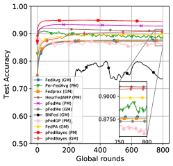
(a)

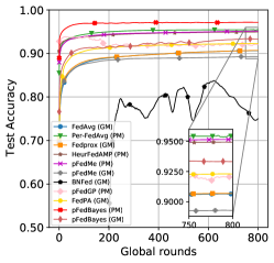
(b)

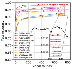
(c)

Figure 4: The convergence curve of the personalization algorithms on the MNIST dataset. Left: Small dataset. Middle: Medium dataset. Right: Large dataset.

Comparison results of the convergence rate of different algorithms on the MNIST dataset.

6 Experiments

6.1 Experimental Setting

We validate the proposed pFedBayes with FedAvg [1], Fedprox [3], BNFed [30], FedPA [31], Per-FedAvg [26], pFedMe [4], HeurFedAMP [9] and pFedGP [32] based on non-i.i.d. and clustering datasets. And the proposed cFedBayes is compared with FedSEM [8], FedCFL [7], IFCA [7]. Three public benchmark datasets, MNIST [42, 43], FMNIST (Fashion-MNIST)[44] and CIFAR-10 [45] are used to generate the non-i.i.d. and clustering datasets. For the MNIST/FMNIST dataset, we used a total of 10 clients, while for the CIFAR-10 dataset, we set up 20 clients. To modify the dataset to be non-i.i.d., a relatively simple approach is to have each client only have a subset of all labels. Here we let each client have only 5 of 10 labels. For clustering datasets, we construct four types, namely MNIST-MNIST^⟂, FMNIST-FMNIST^⟂, MNIST-FMNIST, and CIFAR10-CIFAR10^⟂. MNIST-MNIST^⟂ indicates that this dataset has two cluster categories, the first cluster (corresponding to the first half of clients) is MNIST, and the second cluster (corresponding to the second half of clients) is MNIST^⟂, where $(\cdot)^{\perp}$ represents that the dataset has been reversed operate. The other three clustering datasets are defined similarly. Additionally, we set $S=10$ (random subset of clients) for all experiments. We stop the algorithm at 800 rounds and select the highest accuracy in the last 100 rounds to evaluate the performance of all algorithms.

In addition, in order to verify the performance of the algorithm under different sample sizes, we set three settings of small, medium and large for all datasets. In particular, for MNIST and FMNIST, there are 50 training samples and 950 testing samples per class in the small dataset, 200 training samples and 800 testing samples per class in the medium setting, and 900 training samples and 300 testing samples per class in the large dataset. In contrast, for each class in the CIFAR-10 dataset, we set 25, 100, and 450 training samples and 475, 400, and 150 testing samples for the small, medium, and large settings, respectively.

The computing device we use has two Intel(R) Xeon(R) Gold 6152 CPUs (each with 22 cores, @ 2.10GHz), and two NVIDIA Tesla P100 GPUs with 16GB of memory. The settings of the federated learning environment and the DNN and VGG models are the same as in [4]. Specifically, for the MNIST and FMNIST datasets, we use a DNN model with a hidden layer size of 100. The activation function is ReLU and the network finally passes through the softmax layer. The VGG model [46] is used for the CIFAR-10 dataset with “[16, ‘M’, 32, ‘M’, 64, ‘M’, 128, ‘M’, 128, ‘ M’] ” cfg settings. All experiments are implemented based on PyTorch [47].

6.2 Experimental Hyperparameter Settings

We first study the influence of hyperparameters, and after obtaining the optimal hyperparameters of each algorithm, these algorithms can be compared more fairly. Details of parameter tuning can be found in Appendix B. In general, we conduct parameter tuning studies on the medium MNIST dataset, and perform parameter tuning around the optimal parameters recommended in the original papers of these algorithms. For example, we tune the learning rate from 0.0005 to 0.1, because the optimal learning rate recommended by many algorithms (such as pFedMe) is 0.005. For those non-universal hyperparameters, we directly adopt the optimal values recommended in their papers.

TABLE II: Results of sFedBayes on MNIST, FMNIST and CIFAR-10. Results better than Ours in Table 1 are bolded.

Dataset	Size	Initialized $\lambda$	Estimated $\lambda$	Sparsity ($\%$)	PM (Acc. ($\%$))	GM (Acc. ($\%$))
MNIST	Small	0.50	0.50$\pm$0.00	50.25$\pm$0.21	92.62$\pm$0.14	87.03$\pm$0.59
		0.99	0.98$\pm$0.00	98.32$\pm$0.05	93.28$\pm$0.08	93.28$\pm$0.07
	Medium	0.50	0.50$\pm$0.00	50.16$\pm$0.18	94.70$\pm$0.10	86.97$\pm$0.54
		0.99	0.98$\pm$0.00	98.36$\pm$0.04	97.15$\pm$0.05	95.77$\pm$0.15
	Large	0.50	0.50$\pm$0.00	50.19$\pm$0.20	95.50$\pm$0.13	87.30$\pm$0.45
		0.99	0.98$\pm$0.00	98.37$\pm$0.02	98.63$\pm$0.03	96.37$\pm$0.21
FMNIST	Small	0.50	0.50$\pm$0.00	50.13$\pm$0.18	87.02$\pm$0.02	83.69$\pm$1.15
		0.99	0.88$\pm$0.00	87.56$\pm$0.08	87.64$\pm$0.11	83.62$\pm$0.28
	Medium	0.50	0.50$\pm$0.00	50.18$\pm$0.07	89.21$\pm$0.23	84.58$\pm$0.75
		0.99	0.99$\pm$0.00	98.37$\pm$0.03	91.60$\pm$0.04	86.14$\pm$0.44
	Large	0.50	0.50$\pm$0.00	50.08$\pm$0.17	90.15$\pm$0.05	84.80$\pm$0.73
		0.99	0.99$\pm$0.00	98.39$\pm$0.04	93.07$\pm$0.05	87.96$\pm$0.38
CIFAR-10	Small	0.50	1.01$\pm$0.00	100.00$\pm$0.00	57.84$\pm$0.97	55.23$\pm$1.04
		0.99	1.01$\pm$0.00	100.00$\pm$0.00	56.87$\pm$0.72	54.06$\pm$0.59
	Medium	0.50	1.01$\pm$0.00	100.00$\pm$0.00	77.47$\pm$0.11	76.31$\pm$0.37
		0.99	1.01$\pm$0.00	100.00$\pm$0.00	78.05$\pm$0.19	77.15$\pm$0.30
	Large	0.50	1.01$\pm$0.00	100.00$\pm$0.00	85.43$\pm$0.11	77.02$\pm$1.76
		0.99	1.01$\pm$0.00	100.00$\pm$0.00	85.52$\pm$0.07	79.15$\pm$1.56

According to the tuning results, the learning rates of FedAvg, Per-FedAvg, Fedprox, BNFed, pFedGP and HeurFedAMP as set as 0.01, 0.01, 0.01, 0.5, 0.05 and 0.01, respectively. The personalization and global learning rates are both set to 0.01 for both pFedMe and FedPA. The personalization and global learning rates of pFedBayes, sFedBayes, and cFedBayes are all set to 0.001. The personalization regularization weights for Fedprox, pFedMe, and HeurFedAMP are set to 0.001, 15, and $\alpha=5$, respectively. The personalization regularization weights for pFedBayes, sFedBayes and cFedBayes are all set to $\zeta=10$. The variance of their weights is initialized to $\rho=-2.5$.

6.3 pFedBayes Performance Comparison Results

Table  I shows the detailed performance comparison results of our pFedBayes algorithm and other personalization algorithms. We can see that the personalized model of the proposed pFedBayes has significantly improved performance compared to other algorithms, especially on small datasets. From the third column of Table I, we can see that the personalized model of pFedBayes has improved by 1.69%, 0.7%, and 12.43% compared with other SOTA algorithms on the small MNIST, FMNIST, and CIFAR-10 datasets, respectively. This is because the Bayesian algorithm is more advantageous in small sample conditions, so our pFedBayes converges faster in small datasets. Correspondingly, Figure 4 shows convergence curve of the personalization algorithms on the MNIST dataset. The convergence speed of our pFedBayes is significantly ahead of other algorithms, basically the performance becomes stable after 50 iterations. The experimental results are also consistent with the theory proposed in this paper. Our pFedBayes is an algorithm that achieves the nature of minimax optimality, hence the convergence speed is optimal.

In addition, compared with other algorithms, pFedBayes’ global model has also achieved a leading position in most settings. This shows that our proposed method can aggregate the distribution of the model very well, which is a capability that previous algorithms did not have. Most of the previous algorithms can only aggregate the weight of the model. Some algorithms that try to aggregate the distribution of the model, such as BNFed, do not perform well.

Furthermore, we can also see that the performance improvement of the proposed algorithm on the FMNIST dataset is relatively small, mainly because the FMNIST dataset is simple and the distribution between different labels is relatively close, the performance of the personalization algorithm has no advantage. A simple and robust algorithm like FedAvg will perform better. In contrast, for the complex non-IID CIFAR-10 dataset, the performance improvement of our pFedBayes is significant. Note that on large datasets, our global model does not have much performance advantage. Since for large datasets, BNN usually requires some tricks to achieve the same performance as non-Bayesian algorithms [48]. For fair comparison, we did not add special tricks for large datasets to better compare the most essential performance differences between Bayesian federated learning and other algorithms.

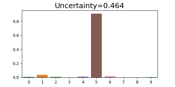
(a)

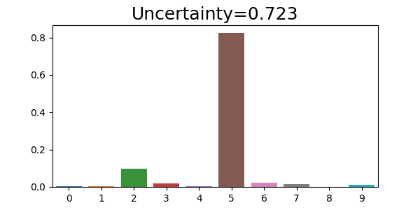
(b)

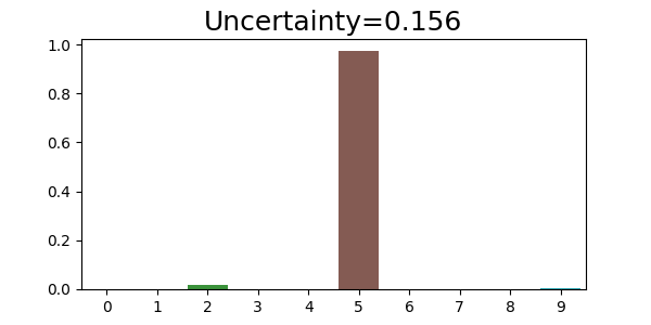
(c)

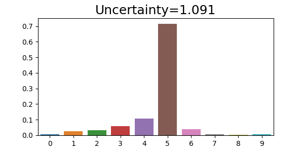
(d)

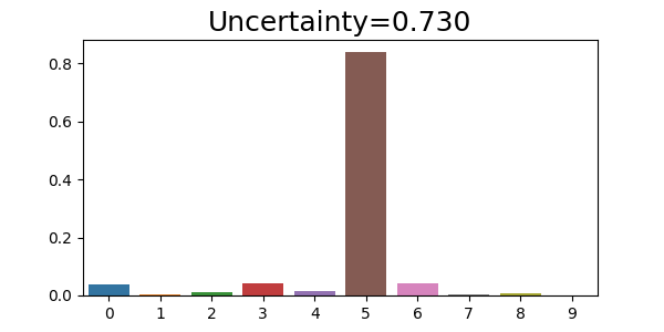
(e)

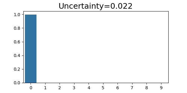
(f)

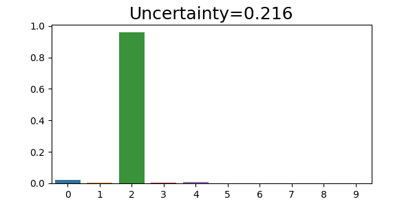
(g)

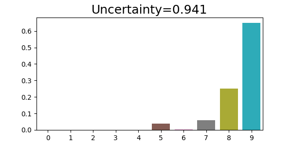
(h)

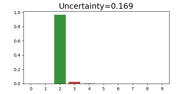
(i)

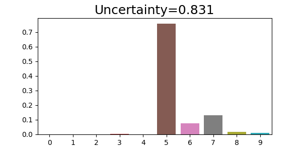
(j)

(k)

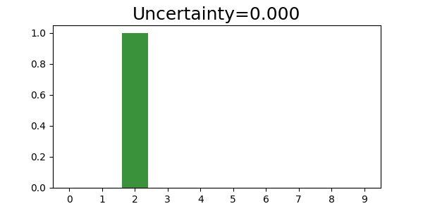
(l)

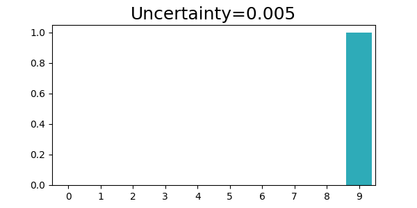
(m)

(n)

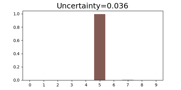
(o)

Figure 5: Prediction uncertainty results for the pFedBayes algorithm. We picked five different clients, and the results of training epochs 0, 1, and 10 are given in rows 1, 2, and 3, respectively.

Finally, our pFedBayes can provide results with uncertainty estimates for each client’s model, which can help federated learning global models choose which models to aggregate. Specifically, when aggregating models, if we know the uncertainty of all models, we also know the quality of the model, that is, we can decide whether to aggregate the model according to the demand. Figure 5 shows the results of the estimation of prediction uncertainty. For randomly initialized models, each client’s uncertainty behaves essentially the same. But as training progresses, each client becomes more confident in its own data classification results. If some models are not confident in their own classification results, we can consider excluding this model during aggregation. Of course, for the sake of fairness, the experiments in this paper did not do so.

6.4 sFedBayes Performance Comparison Results

Table II shows the performance of sFedBayes on small, medium and large datasets of MNIST, FMNIST and CIFAR-10. We can see that after initializing the $\lambda$, we can control the sparsity of the model. On the MNIST and FMNIST datasets, the value of $\lambda$ corresponds to the sparsity at the end of training. This is because the MNIST and FMNIST datasets are relatively simple, and the sparse model can also learn good results, so the algorithm allows the model to become very sparse. In contrast, on the CIFAR-10 dataset, the sparse model is not enough to learn good results, so as the training progresses, the model will become less and less sparse, and the final learned results are not sparse.

In addition, the accuracy of the model can be improved after the model is sparse. The results in Table II that are better than our non-sparse model in Table I are all bolded. We can see that most of the global models, especially, have improved accuracy, and the personalized model and the global model are improved by up to 4.11% (CIFAR-10 Medium) and 14.75% (CIFAR-10 Large), respectively. We speculate that this is because sparse models at the beginning can speed up convergence, and sparse models are more resistant to overfitting.

Another benefit of sparsification is that it can reduce the amount of communication between the cloud and clients. For example, we can set a threshold tol, and when an neural with $\lambda<\text{tol}$, its parameters will not be transmitted, so that many transmission parameters can be reduced.

TABLE III: Clustering Results on MNIST, FMNIST and CIFAR-10. Best results are bolded.

Dataset	Method	Small (Acc. ($\%$))		Medium (Acc. ($\%$))		Large (Acc. ($\%$))
		PM	GM	PM	GM	PM	GM
MNIST-MNIST⟂	FeSEM [8]	-	77.67$\pm$1.73	-	85.67$\pm$2.08	-	90.68$\pm$2.01
	FedCFL [7]	-	68.41$\pm$3.76	-	79.54$\pm$3.76	-	72.63$\pm$8.06
	IFCA [7]	-	53.70$\pm$0.00	-	19.80$\pm$0.00	-	58.40$\pm$0.00
	Ours	91.19$\pm$0.10	78.88$\pm$0.74	95.51$\pm$0.10	83.23$\pm$1.44	97.94$\pm$0.05	83.39$\pm$2.10
FMNIST-FMNIST⟂	FeSEM [8]	-	79.14$\pm$0.90	-	81.13$\pm$1.49	-	85.56$\pm$1.88
	FedCFL [7]	-	36.82$\pm$5.63	-	48.65$\pm$8.55	-	48.91$\pm$5.06
	IFCA [7]	-	59.40$\pm$0.00	-	59.10$\pm$0.00	-	60.80$\pm$0.00
	Ours	85.99$\pm$0.05	79.28$\pm$2.40	89.82$\pm$0.27	81.20$\pm$1.10	91.70$\pm$0.09	82.55$\pm$2.68
MNIST-FMNIST	FeSEM [8]	-	81.72$\pm$1.89	-	83.47$\pm$2.61	-	85.47$\pm$2.58
	FedCFL [7]	-	64.86$\pm$5.47	-	72.36$\pm$4.91	-	72.74$\pm$4.33
	IFCA [7]	-	54.80$\pm$0.00	-	35.20$\pm$0.00	-	54.40$\pm$0.00
	Ours	89.31$\pm$0.09	82.46$\pm$1.12	93.06$\pm$0.08	86.47$\pm$1.41	95.41$\pm$0.04	87.20$\pm$2.25
CIFAR10-CIFAR10⟂	FeSEM [8]	-	42.63$\pm$2.13	-	52.98$\pm$0.88	-	62.63$\pm$0.59
	FedCFL [7]	-	38.53$\pm$0.84	-	52.39$\pm$2.03	-	68.09$\pm$1.24
	IFCA [7]	-	48.60$\pm$0.00	-	51.00$\pm$0.50	-	51.70$\pm$0.00
	Ours	55.67$\pm$1.28	43.34$\pm$2.78	70.29$\pm$0.17	50.82$\pm$2.87	77.81$\pm$0.24	58.03$\pm$4.18

6.5 cFedBayes Performance Comparison Results

Table III shows the performance comparison results of cFedBayes on small, medium and large clustering datasets. For other comparison algorithms, they don’t have dedicated personalization models. We use the only model as the global model and calculate the average accuracy across all clusters. We can see that the accuracy of the personalized model obtained by our cFedBayes is far ahead of the accuracy of other algorithms, and it is also far ahead of the accuracy of our global model. The model accuracy can be improved up to 17.31% (CIFAR10-CIFAR10^⟂ Medium). Moreover, the accuracy of our global model leads other clustering algorithms in most cases, which also shows the power of the proposed cFedBayes algorithm.

7 Conclusions

This paper proposes three novel personalized Bayesian federated learning models via variational inference when the data is limited. We first propose pFedBayes to achieve personalization under Gaussian distributions. Then we propose sFedBayes to simplify the network structure. Finally, we propose cFedBayes to address the extreme statistical diversity among clients. The average generalization error bounds are provided for the three approaches, which demonstrates that the proposed methods achieve the minimax optimal convergence rate. Numerical results illustrate that the proposed methods outperform existing advanced personalized methods under non-i.i.d. limited data.

There are several interesting directions for future work. One is to provide the convergence analysis for the proposed methods. One is to study the clustered federated learning model with an unknown number of clusters. The other is to extend the proposed methods to decentralized settings where only local communications are allowed.

Appendix A Proof of Lemmas

A.1 Proof of Lemma 1

Before giving the proof of Lemma 1, we present the following useful lemma for KL divergence [49].

Lemma A.1.

Given arbitrary probability measure $\mu$ and arbitrary measurable function $h$ with $e^{h}\in L_{1}(\mu)$, we have

$$\log\int e^{h(\eta)}\mu(d\eta)=\sup_{\rho}\left[\int h(\eta)\rho(d\eta)-\mbox{\rm KL}(\rho||\mu)\right].$$

We start to prove Lemma 1. Choosing $\log\eta(P^{i}_{\bm{\theta}},P^{i})=l_{n}(P^{i}_{\bm{\theta}},P^{i})/\zeta+n\,d^{2}(P^{i}_{\bm{\theta}},P^{i})$ with $\zeta\geq 1$, then we have

$$\mathbb{E}_{P^{i}}\exp(l_{n}(P^{i}_{\bm{\theta}},P^{i})/\zeta) =\mathbb{E}_{P^{i}}\left(\frac{p^{i}_{\bm{\theta}}(\bm{D}^{i})}{p^{i}(\bm{D}^{i})}\right)^{\frac{1}{\zeta}}$$

$$\leq\left(\mathbb{E}_{P^{i}}\frac{p^{i}_{\bm{\theta}}(\bm{D}^{i})}{p^{i}(\bm{D}^{i})}\right)^{\frac{1}{\zeta}}=1,$$ (A.1)

where the inequality follows Jensen’s inequality and the concavity of $(\cdot)^{1/\zeta}$.

Combining with the proof from the Theorem 3.1 of [50], the following inequality holds with high probability

$$\int_{\Theta}\eta(P^{i}_{\bm{\theta}},P^{i})w^{\star}(\bm{\theta})d\bm{\theta}\leq e^{Cn\varepsilon^{2}_{n}},$$ (A.2)

where $C>0$ is a large enough constant.

Choosing $h(\eta)=\log\eta(P^{i}_{\bm{\theta}},P^{i})$, $\mu=w^{\star}(\bm{\theta})$ and $\rho=\hat{q}^{i}(\bm{\theta})$ in Lemma A.1, we have

$$\int_{\Theta}d^{2}(P_{\bm{\theta}}^{i},P^{i})\hat{q}^{i}(\bm{\theta})d\bm{\theta}$$

$$\leq \frac{1}{n}\bigg{[}\frac{1}{\zeta}\int_{\Theta}l_{n}(P^{i},P^{i}_{\bm{\theta}})\hat{q}^{i}(\bm{\theta})d\bm{\theta}+\mbox{KL}(\hat{q}^{i}(\bm{\theta})||w^{\star}(\bm{\theta}))$$

$$\quad+\log\int_{\Theta}\eta(P^{i}_{\bm{\theta}},P^{i})w^{\star}(\bm{\theta})d\bm{\theta}\bigg{]}$$

$$\leq \frac{1}{n}\left[\frac{1}{\zeta}\int_{\Theta}l_{n}(P^{i},P^{i}_{\bm{\theta}})\hat{q}^{i}(\bm{\theta})d\bm{\theta}+\mbox{KL}(\hat{q}^{i}(\bm{\theta})||w^{\star}(\bm{\theta}))\right]+C\varepsilon^{2}_{n}.$$ (A.3)

By taking the average of all $N$ clients, we finish the proof:

$$\frac{1}{N}\sum_{i=1}^{N}\int_{\Theta}d^{2}(P_{\bm{\theta}}^{i},P^{i})\hat{q}^{i}(\bm{\theta})d\bm{\theta}\\ \leq\frac{1}{n}\bigg{\{}\frac{1}{N}\sum_{i=1}^{N}\Big{[}\frac{1}{\zeta}\int_{\Theta}l_{n}(P^{i},P^{i}_{\bm{\theta}})\hat{q}^{i}(\bm{\theta})d\bm{\theta}\\ +\mbox{KL}(\hat{q}^{i}(\bm{\theta})||w^{\star}(\bm{\theta}))\Big{]}\bigg{\}}+C\varepsilon^{2}_{n}.$$ (A.4)

A.2 Proof of Lemma 2

We begin the proof of Lemma 2 by giving Lemma A.2, which shows the relationship of the optimal global distribution $w(\bm{\theta})$ and the distributions of all clients $\{q^{i}(\bm{\theta})\}_{i=1}^{N}$. The proof of Lemma A.2 is delayed in Section A.5.

Lemma A.2.

Let $w(\bm{\theta})$ be the solution of the following problem

$$\min_{w(\bm{\theta})}\left\{F(w)=\frac{1}{N}\sum_{i=1}^{N}\mbox{\rm KL}(q^{i}(\bm{\theta})||w(\bm{\theta})))\right\}.$$ (A.5)

Then the following equations hold

$$\mu_{w,m} =\frac{1}{N}\sum_{i=1}^{N}\mu_{i,m},$$ (A.6)

$$\sigma_{w,m}^{2} =\frac{1}{N}\sum_{i=1}^{N}\left[\sigma_{i,m}^{2}+\left(\mu_{i,m}-\mu_{w,m}\right)^{2}\right].$$ (A.7)

Next, we present the proof of Lemma 2. Let $\bm{\theta}^{\star}_{i}$ be the minimizer of $\left\lVert f^{i}_{\bm{\theta}}-f^{i}\right\rVert^{2}_{\infty}$ subject to $\left\lVert\bm{\theta}\right\rVert_{\infty}\leq B$ and define the local distribution $\tilde{q}^{i}(\bm{\theta})$ of the $i$-th client:

$$\begin{split}&\theta_{i,m}\sim\mathcal{N}(\theta_{i,m}^{\star},\sigma^{2}_{n}),m=1,\dots,T\end{split}$$ (A.8)

where $\sigma_{n}^{2}$ follows Assumption 3, i.e., $\sigma_{n}^{2}=\frac{T}{8n}A$ and

$$A=\log^{-1}(3r_{0}M)\cdot(2BM)^{-2(L+1)}\bigg{[}\Big{(}r_{0}+1+\frac{1}{BM-1}\Big{)}^{2}\\ +\frac{1}{(2BM)^{2}-1}+\frac{2}{(2BM-1)^{2}}\bigg{]}^{-1}.$$ (A.9)

Let $\tilde{w}(\bm{\theta})$ represent the solution of

$$\min_{w(\bm{\theta})\in\mathcal{Q}}\frac{1}{N}\sum_{i=1}^{N}\mbox{KL}(\tilde{q}^{i}(\bm{\theta})||w(\bm{\theta}))).$$ (A.10)

Lemma A.2 presents that the distribution $\tilde{w}(\bm{\theta})$ appears as

$$\theta_{\tilde{w},m}\sim\mathcal{N}(\mu_{\tilde{w},m},\sigma^{2}_{\tilde{w},m}),m=1,\ldots,T,$$ (A.11)

where

$$\mu_{\tilde{w},m} =\frac{1}{N}\sum_{i=1}^{N}\theta_{i,m}^{\star},$$ (A.12)

$$\sigma_{\tilde{w},m}^{2} =\frac{1}{N}\sum_{i=1}^{N}\left[\sigma_{n}^{2}+\left(\theta_{i,m}^{\star}-\mu_{\tilde{w},m}\right)^{2}\right].$$ (A.13)

Using the optimality of $w^{\star}(\bm{\theta})$ and $\hat{q}(\bm{\theta})$ implies

$$\frac{1}{N}\sum_{i=1}^{N}\left[\int_{\Theta}l_{n}(P^{i},P^{i}_{\bm{\theta}})\hat{q}^{i}(\bm{\theta})d\bm{\theta}+\zeta\,\mbox{KL}(\hat{q}^{i}(\bm{\theta})||w^{\star}(\bm{\theta}))\right]\\ \leq\frac{1}{N}\sum_{i=1}^{N}\left[\int_{\Theta}l_{n}(P^{i},P^{i}_{\bm{\theta}})\tilde{q}^{i}(\bm{\theta})d\bm{\theta}+\zeta\,\mbox{KL}(\tilde{q}^{i}(\bm{\theta})||\tilde{w}(\bm{\theta}))\right].$$ (A.14)

Then we give the upper bound of the right-hand side. Under the assumptions of mean-field decomposition, we have

$$\tilde{q}^{i}(\bm{\theta}) =\prod^{T}_{m=1}\mathcal{N}(\theta^{\star}_{i,m},\sigma^{2}_{n}),$$ (A.15)

$$\tilde{w}(\bm{\theta}) =\prod^{T}_{m=1}\mathcal{N}(\mu_{\tilde{w},m},\sigma^{2}_{\tilde{w},m}).$$ (A.16)

Therefore,

$$\mbox{KL}(\tilde{q}^{i}(\bm{\theta})||\tilde{w}(\bm{\theta}))$$

$$= \mbox{KL}\left(\prod^{T}_{m=1}\mathcal{N}(\theta^{\star}_{i,m},\sigma^{2}_{n})\Bigl{|}\Bigr{|}\prod^{T}_{m=1}\mathcal{N}(\mu_{\tilde{w},m},\sigma^{2}_{\tilde{w},m})\right)$$

$$= \sum^{T}_{m=1}\mbox{KL}\left(\mathcal{N}(\theta^{\star}_{i,m},\sigma^{2}_{n})||\mathcal{N}(\mu_{\tilde{w},m},\sigma^{2}_{\tilde{w},m})\right)$$

$$= \frac{1}{2}\sum^{T}_{m=1}\left[\log\Bigl{(}\frac{\sigma^{2}_{\tilde{w},m}}{\sigma^{2}_{n}}\Bigr{)}+\frac{\sigma^{2}_{n}+(\theta^{\star}_{i,m}-\mu_{\tilde{w},m})^{2}}{\sigma^{2}_{\tilde{w},m}}-1\right]$$

$$= \frac{1}{2}\sum^{T}_{m=1}\left[\log\Bigl{(}\frac{\sigma^{2}_{\tilde{w},m}}{\sigma^{2}_{n}}\Bigr{)}-1\right]+\frac{1}{2}\sum^{T}_{m=1}\frac{\sigma^{2}_{n}+(\theta^{\star}_{i,m}-\mu_{\tilde{w},m})^{2}}{\sigma^{2}_{\tilde{w},m}}$$

$$\leq \frac{T}{2}\left[\log\left(\frac{\sigma^{2}_{n}+B^{2}}{\sigma^{2}_{n}}\right)-1\right]+\frac{1}{2}\sum^{T}_{m=1}\frac{\sigma^{2}_{n}+(\theta^{\star}_{i,m}-\mu_{\tilde{w},m})^{2}}{\sigma^{2}_{\tilde{w},m}},$$ (A.17)

where the last inequality follows

$$\sigma_{\tilde{w},m}^{2}=\sigma_{n}^{2}-\mu_{\tilde{w},m}^{2}+\frac{1}{N}\sum_{i=1}^{N}\theta_{i,m}^{\star 2}\leq\sigma^{2}_{n}+B^{2}.$$

By summing over all clients, we obtain

$$\frac{1}{N}\sum_{i=1}^{N}\mbox{KL}(\tilde{q}^{i}(\bm{\theta})||\tilde{w}(\bm{\theta}))\leq \frac{1}{N}\sum_{i=1}^{N}\bigg{\{}\frac{T}{2}\left[\log\left(\frac{\sigma^{2}_{n}+B^{2}}{\sigma^{2}_{n}}\right)-1\right]$$

$$+\frac{1}{2}\sum^{T}_{m=1}\frac{\sigma^{2}_{n}+(\theta^{\star}_{i,m}-\mu_{\tilde{w},m})^{2}}{\sigma^{2}_{\tilde{w},m}}\bigg{\}}$$

$$\leq \frac{T}{2}\log\left(\frac{\sigma^{2}_{n}+B^{2}}{\sigma^{2}_{n}}\right),$$

where the last inequality follows (A.13), i.e.,

$$\frac{1}{N}\sum_{i=1}^{N}\frac{\sigma^{2}_{n}+(\theta^{\star}_{i,m}-\mu_{\tilde{w},m})^{2}}{\sigma^{2}_{\tilde{w},m}}=1.$$

Using Assumption 3 yields

$$\frac{1}{N}\sum_{i=1}^{N}\mbox{KL}(\tilde{q}^{i}(\bm{\theta})||\tilde{w}(\bm{\theta}))\leq\frac{T}{2}\log\left(\frac{2B^{2}}{\sigma^{2}_{n}}\right).$$ (A.18)

According to the definition of $\sigma_{n}$ (10), we have

$$\frac{T}{2}\log\left(\frac{2B^{2}}{\sigma^{2}_{n}}\right)\leq T(L+1)\log(2BM)+\frac{T}{2}\log\log(3r_{0}M)\\ +T\log\left(4r_{0}\sqrt{\frac{n}{T}}\right)+\frac{T}{2}\log(2B^{2})\leq C^{\prime}n\chi_{n}.$$ (A.19)

Combining Eqs. (A.18) and (A.19) gets

$$\frac{1}{N}\sum_{i=1}^{N}\mbox{KL}(\tilde{q}^{i}(\bm{\theta})||\tilde{w}(\bm{\theta}))\leq C^{\prime}n\chi_{n}.$$ (A.20)

Using the technique from the Supplementary of [38], we obtain

$$\int_{\Theta}l_{n}(P^{i},P^{i}_{\bm{\theta}})\tilde{q}^{i}(\bm{\theta})d\bm{\theta}\leq C^{\prime\prime}(n\chi_{n}+n\xi^{i}_{n}).$$ (A.21)

Since $\zeta\geq 1$, we get the final upper bound

$$\frac{1}{N}\sum_{i=1}^{N}\left[\int_{\Theta}l_{n}(P^{i},P^{i}_{\bm{\theta}})\hat{q}^{i}(\bm{\theta})d\bm{\theta}+\zeta\,\mbox{KL}(\hat{q}^{i}(\bm{\theta})||w^{\star}(\bm{\theta}))\right]\\ \leq n\left(C^{\prime}\zeta\chi_{n}+\frac{C^{\prime\prime}}{N}\sum_{i=1}^{N}\xi^{i}_{n}\right).$$ (A.22)

A.3 Proof of Lemma 3

Choosing $\log\eta(P^{i}_{\bm{\theta}},P^{i})=l_{n}(P^{i}_{\bm{\theta}}P^{i})/\zeta+n\,d^{2}(P^{i}_{\bm{\theta}},P^{i})$ with $\zeta\geq 1$ and Using (A.1) gives

$$\mathbb{E}_{P^{i}}\exp(l_{n}(P^{i}_{\bm{\theta}},P^{i})/\zeta)\leq 1.$$ (A.23)

Combining with the proof from the Theorem 3.1 of [50], we have

$$\int_{\Theta}\eta(P^{i}_{\bm{\theta}},P^{i})\hat{w}^{k}(\bm{\theta})d\bm{\theta}\leq e^{Cn\varepsilon^{2}_{n}},\,\mbox{w.h.p.,}$$ (A.24)

where $C>0$ is a large number.

By choosing $h(\eta)=\log\eta(P^{i}_{\bm{\theta}},P^{i})$, $\mu=\hat{w}^{k}(\bm{\theta})$ and $\rho=\hat{q}^{i}(\bm{\theta})$ in Lemma A.1, for any $k=1,\ldots,K$, we obtain

$$\int_{\Theta}d^{2}(P_{\bm{\theta}}^{i},P^{i})\hat{q}^{i}(\bm{\theta})d\bm{\theta}$$

$$\leq \frac{1}{n}\bigg{[}\frac{1}{\zeta}\int_{\Theta}l_{n}(P^{i},P^{i}_{\bm{\theta}})\hat{q}^{i}(\bm{\theta})d\bm{\theta}+\mbox{KL}(\hat{q}^{i}(\bm{\theta})||\hat{w}^{k}(\bm{\theta}))$$

$$\quad+\log\int_{\Theta}\eta(P^{i}_{\bm{\theta}},P^{i})\hat{w}^{k}(\bm{\theta})d\bm{\theta}\bigg{]}$$

$$\leq \frac{1}{n}\left[\frac{1}{\zeta}\int_{\Theta}l_{n}(P^{i},P^{i}_{\bm{\theta}})\hat{q}^{i}(\bm{\theta})d\bm{\theta}+\mbox{KL}(\hat{q}^{i}(\bm{\theta})||\hat{w}^{k}(\bm{\theta}))\right]+C\varepsilon^{2}_{n}.$$ (A.25)

To give a tight upper bound, $k=\hat{k}^{i}$ is the one that minimizes the KL divergence $\mbox{KL}(\hat{q}^{i}(\bm{\theta})||\hat{w}^{k}(\bm{\theta}))$. Therefore,

$$\int_{\Theta}d^{2}(P_{\bm{\theta}}^{i},P^{i})\hat{q}^{i}(\bm{\theta})d\bm{\theta}$$

$$\leq \frac{1}{n}\Bigg{\{}\frac{1}{\zeta}\int_{\Theta}l_{n}(P^{i},P^{i}_{\bm{\theta}})\hat{q}^{i}(\bm{\theta})d\bm{\theta}+\mbox{\rm KL}(\hat{q}^{i}(\bm{\theta})||\hat{w}^{\hat{k}^{i}}(\bm{\theta}))\Bigg{\}}+C\varepsilon^{2}_{n}.$$ (A.26)

A.4 Proof of Lemma 4

Before proving Lemma 4, we present a corollary of Lemma A.2 to the optimal parameters of the distribution $w^{k}(\bm{\theta})$ for fixed distributions of all clients $\{q^{i}(\bm{\theta})\}_{i\in\mathbb{T}_{k}}$ in the $k$-th cluster.

Lemma A.3.

Let $\mathbb{T}_{k}$ be the index set of clients that belong to the $k$-th cluster. Let $w^{k}(\bm{\theta})$ be the solution of the following problem

$$\min_{w^{k}(\bm{\theta})}\left\{F(w^{k})=\frac{1}{\mathbb{T}_{k}}\sum_{i\in\mathbb{T}_{k}}\mbox{\rm KL}(q^{i}(\bm{\theta})||w^{k}(\bm{\theta})))\right\}.$$ (A.27)

Then we have

$$\mu_{w^{k},m} =\frac{1}{\mathbb{T}_{k}}\sum_{i\in\mathbb{T}_{k}}\mu_{i,m},$$ (A.28)

$$\sigma_{w,m}^{2} =\frac{1}{\mathbb{T}_{k}}\sum_{i\in\mathbb{T}_{k}}\left[\sigma_{i,m}^{2}+\mu_{i,m}^{2}-\mu_{w^{k},m}^{2}\right].$$ (A.29)

Due to the definition of $\mathbb{S}_{k}$, we have

$${\hat{k}^{i}}=k,i\in\mathbb{S}_{k}.$$ (A.30)

So the left-hand term in (50) is equivalent to

$$\frac{1}{|\mathbb{S}_{k}|}\sum_{i\in\mathbb{S}_{k}}\Bigg{[}\int_{\Theta}l_{n}(P^{i},P^{i}_{\bm{\theta}})\hat{q}^{i}(\bm{\theta})d\bm{\theta}+\zeta\,\mbox{\rm KL}(\hat{q}^{i}(\bm{\theta})||\hat{w}^{k}(\bm{\theta}))\Bigg{]}$$ (A.31)

Then by following the techniques from the proof of Lemma 2, it’s straightforward to get Lemma 4.

A.5 Proof of Lemma A.2

The optimality of $w(\bm{\theta})$ in Eq. (A.27) implies that the one-order partial derivatives of $F(w)$ w.r.t. $\mu_{w,m}$ and $\sigma_{w,m}$ are zero

$$\frac{1}{N}\sum_{i=1}^{N}\frac{\partial\,\mbox{KL}(q^{i}(\bm{\theta})||w(\bm{\theta}))}{\partial\,\mu_{w,m}} =0,$$ (A.32)

$$\frac{1}{N}\sum_{i=1}^{N}\frac{\partial\,\mbox{KL}(q^{i}(\bm{\theta})||w(\bm{\theta}))}{\partial\,\sigma_{w,m}} =0.$$ (A.33)

Using Eq. (3) yields

$$\frac{1}{N}\sum_{i=1}^{N}\frac{\partial\,\mbox{KL}(q^{i}(\bm{\theta})||w(\bm{\theta}))}{\partial\,\mu_{w,m}}=\frac{1}{N}\sum_{i=1}^{N}\frac{-2(\mu_{i,m}-\mu_{w,m})}{\sigma_{w,m}^{2}},$$ (A.34)

and

$$\frac{1}{N}\sum_{i=1}^{N}\frac{\partial\,\mbox{KL}(q^{i}(\bm{\theta})||w(\bm{\theta}))}{\partial\,\sigma_{w,m}}\\ =\frac{1}{N}\sum_{i=1}^{N}\left[\frac{2}{\sigma_{w,m}}-\frac{2\left[\sigma_{i,m}^{2}+\left(\mu_{i,m}-\mu_{w,m}\right)^{2}\right]}{\sigma_{w,m}^{3}}\right].$$ (A.35)

Therefore, we obtain

$$\mu_{w,m} =\frac{1}{N}\sum_{i=1}^{N}\mu_{i,m},$$ (A.36)

$$\sigma_{w,m}^{2} =\frac{1}{N}\sum_{i=1}^{N}\left[\sigma_{i,m}^{2}+\left(\mu_{i,m}-\mu_{w,m}\right)^{2}\right]$$ (A.37)

TABLE IV: Results of pFedBayes on Medium dataset (MNIST).

$\rho$	$\zeta$	$\eta_{1}$	$\eta_{2}$	PM Acc.($\%$)	GM Acc.($\%$)
-1	10	0.001	0.001	97.38	91.61
-1	10	0.001	0.005	97.12	90.32
-1	10	0.005	0.001	96.73	91.34
-1	10	0.005	0.005	96.78	91.10
-2	10	0.001	0.001	97.45	92.40
-2	10	0.001	0.005	97.42	91.35
-2	10	0.005	0.001	97.36	91.27
-2	10	0.005	0.005	97.28	90.01
-3	10	0.001	0.001	97.08	92.16
-3	10	0.001	0.005	96.35	90.47
-3	10	0.005	0.001	96.64	87.34
-3	10	0.005	0.005	97.28	90.22
-1.5	10	0.001	0.001	97.38	92.31
-2.0	10	0.001	0.001	97.45	92.40
-2.5	10	0.001	0.001	97.18	93.22
-2.5	0.5	0.001	0.001	97.13	89.88
-2.5	1	0.001	0.001	97.41	91.24
-2.5	5	0.001	0.001	97.38	93.03
-2.5	10	0.001	0.001	97.18	93.22
-2.5	20	0.001	0.001	97.04	92.77

TABLE V: Results of sFedBayes on Medium dataset (MNIST).

$\rho$	$\zeta$	$\lambda$	Sparsity	PM Acc.($\%$)	GM Acc.($\%$)
-2.5	10	0.10	0.0994	55.23	39.84
-2.5	10	0.30	0.3023	87.81	71.00
-2.5	10	0.50	0.5027	93.86	82.75
-2.5	10	0.75	0.6725	95.85	87.64
-2.5	10	0.80	0.7986	96.68	91.08
-2.5	10	0.90	0.9855	97.23	95.15
-2.5	10	0.99	0.9829	97.34	95.12

Appendix B Experimental Results on MNIST Dataset

B.1 Effect of Hyperparameters

We validate pFedBayes and sFedBayes in a basic DNN model with 3 full connection layers [784, 100, 10] on the MNIST Medium dataset, the results are listed in Table IV and Table V, respectively. Effects of $\eta_{1}$ and $\eta_{2}$: In the pFedBayes algorithm, $\eta_{1}$ and $\eta_{2}$ represent the learning rates of the personalized model and the global model, respectively. We tune the learning rate in the range $[0.001,0.005]$ while fixing other parameters. Table IV shows that $\eta_{1}=\eta_{2}=0.001$ is the best learning rate setting. Effects of $\zeta$: In the pFedBayes algorithm, $\zeta$ can adjust the degree of personalization. Therefore, increasing $\zeta$ can improve the performance of the global model, but weaken the performance of the personalized model. Based on the optimal learning rate, we tune $\zeta\in\{0.5,1,5,10,20\}$. From Table IV we can see that $\zeta=10$ is the best setting. As a result, $\zeta=10$ is used for the remaining experiments. Effects of $\rho$: Note that the initialization of weight parameters can affect the results of the model. Therefore, we also tune $\rho\in\{-1,-1.5,-2,-2.5,-3\}$. From Table IV we can see that $\rho=-2.5$ is the optimal setting. We set $\rho=-2.5$ for the remaining experiments. Effects of $\lambda$: The value of $\lambda$ represents the initialized sparsity of the model. By controlling $\lambda$, the sparsity of the model can be controlled. However, as the training progresses, the sparsity of the model may change to a certain extent. As can be seen from Table V, a certain degree of sparsity can speed up model convergence and avoid problems such as overfitting. But when the model is too sparse, the performance will regress.

TABLE VI: Results of FedAvg, Fedprox, and BNFed on Medium dataset (MNIST). $\eta_{1}$ and $\eta_{2}$ are the personalized model and global model learning rate, respectively.

Algorithm	$\eta_{1}$	$\eta_{2}$	$\lambda$	PM Acc.($\%$)	GM Acc.($\%$)
FedAvg	-	0.0005	-	-	87.65
FedAvg	-	0.001	-	-	89.19
FedAvg	-	0.005	-	-	90.08
FedAvg	-	0.01	-	-	90.66
FedAvg	-	0.1	-	-	90.34
Fedprox	-	0.001	0.001	-	89.26
Fedprox	-	0.001	0.01 -	-	89.24
Fedprox	-	0.001	0.1	-	87.79
Fedprox	-	0.001	1	-	76.79
Fedprox	-	0.0005	0.001	-	87.64
Fedprox	-	0.001	0.001	-	89.26
Fedprox	-	0.005	0.001	-	89.84
Fedprox	-	0.01	0.001	-	90.70
Fedprox	-	0.1	0.001	-	21.31
BNFed	-	0.0005	-	-	9.90
BNFed	-	0.001	-	-	9.90
BNFed	-	0.005	-	-	9.90
BNFed	-	0.01	-	-	9.94
BNFed	-	0.1	-	-	55.98
BNFed	-	0.2	-	-	74.47
BNFed	-	0.5	-	-	80.31

TABLE VII: Results of pFedMe, FedPA on Medium dataset (MNIST). $\eta_{1}$ and $\eta_{2}$ are the personalized model and global model learning rate of the algorithm, respectively.

Algorithm	$\eta_{1}$	$\eta_{2}$	$\lambda$	PM Acc.($\%$)	GM Acc.($\%$)
pFedMe	0.0005	0.001	15	83.22	80.86
pFedMe	0.001	0.001	15	89.35	86.86
pFedMe	0.005	0.005	15	94.35	89.17
pFedMe	0.01	0.01	15	95.16	89.31
pFedMe	0.1	0.1	15	19.73	9.9
FedPA	0.0005	0.001	-	-	81.45
FedPA	0.001	0.001	-	-	81.89
FedPA	0.005	0.005	-	-	90.21
FedPA	0.01	0.01	-	-	92.44
FedPA	0.1	0.1	-	-	44.71

TABLE VIII: Results of HeurFedAMP, Per-FedAvg and pFedGP on Medium dataset (MNIST). $\eta_{1}$ and $\eta_{2}$ are the personalized model and global model learning rate, respectively.

Algorithm	$\eta_{1}$	$\eta_{2}$	$\alpha$	PM Acc.($\%$)	GM Acc.($\%$)
HeurFedAMP	0.0005	-	0.1	89.73	-
HeurFedAMP	0.001	-	0.1	89.91	-
HeurFedAMP	0.005	-	0.1	89.41	-
HeurFedAMP	0.01	-	0.1	88.68	-
HeurFedAMP	0.1	-	0.1	87.51	-
HeurFedAMP	0.0005	-	0.5	93.32	-
HeurFedAMP	0.001	-	0.5	94.04	-
HeurFedAMP	0.005	-	0.5	94.90	-
HeurFedAMP	0.01	-	0.5	94.95	-
HeurFedAMP	0.1	-	0.5	94.86	-
Per-FedAvg	0.0005	-	-	94.71	-
Per-FedAvg	0.001	-	-	94.95	-
Per-FedAvg	0.005	-	-	95.31	-
Per-FedAvg	0.01	-	-	95.35	-
Per-FedAvg	0.1	-	-	19.94	-
pFedGP	0.01	-	-	90.52	-
pFedGP	0.05	-	-	92.14	-
pFedGP	0.1	-	-	91.23	-

The results of FedAvg, Fedprox, BNFed, pFedMe, FedPA, HeurFedAMP, Per-FedAvg and pFedGP are listed in Tables VI-VIII. For a fair comparison with these algorithms, we perform the following hyperparameter tuning. According to [4], $\lambda=15$ achieves the best performance of the pFedMe algorithm, hence we directly use it in our experiments. For Fedprox, we tune $\lambda\in\{0.001,0.01,0.1,1\}$ the same as the setting in [3]. As for HeurFedAMP, $0.5$ is the recommended setting in [9], and we tune $\alpha\in[0.1,0.5]$. Note that $\alpha$ represents the proportion of the client model that does not interact with the global model. Higher values result in less interaction with the global model. For a fair comparison with other algorithms, $\alpha$ should be set to 0.1 since there are 10 client models interacting with the global model. Apparently 0.5 provides better personalization model performance, although the setting of 0.5 is not a fair comparison. We still use the parameter setting 0.5 recommended in the original paper. As for pFedGP, the recommended learning rate in the paper [32] is 0.05, so we tune $\eta\in[0.01,0.05,0.1]$. The result shows that $\eta=0.05$ achieves the best performance. For other hyperparameters in pFedGP, we set them the same as in [32]. As for the learning rate, it is noteworthy that it cannot be set too large. For most federated learning algorithms, an excessively large learning rate will cause the model to diverge, resulting in a serious loss of model aggregation performance.

References

- [1] B. McMahan, E. Moore, D. Ramage, S. Hampson, and B. A. y Arcas, “Communication-efficient learning of deep networks from decentralized data,” in Artificial Intelligence and Statistics. PMLR, 2017, pp. 1273–1282.
- [2] T. Li, A. K. Sahu, A. Talwalkar, and V. Smith, “Federated learning: Challenges, methods, and future directions,” IEEE Signal Processing Magazine, vol. 37, no. 3, pp. 50–60, 2020.
- [3] T. Li, A. K. Sahu, M. Zaheer, M. Sanjabi, A. Talwalkar, and V. Smith, “Federated optimization in heterogeneous networks,” arXiv preprint arXiv:1812.06127, 2018.
- [4] C. T Dinh, N. Tran, and T. D. Nguyen, “Personalized federated learning with moreau envelopes,” Advances in Neural Information Processing Systems, vol. 33, 2020.
- [5] F. Hanzely and P. Richtárik, “Federated learning of a mixture of global and local models,” arXiv preprint arXiv:2002.05516, 2020.
- [6] Y. Li, X. Liu, X. Zhang, Y. Shao, Q. Wang, and Y. Geng, “Personalized federated learning via maximizing correlation with sparse and hierarchical extensions,” arXiv preprint arXiv:2107.05330, 2021.
- [7] A. Ghosh, J. Chung, D. Yin, and K. Ramchandran, “An efficient framework for clustered federated learning,” Advances in Neural Information Processing Systems, vol. 33, pp. 19 586–19 597, 2020.
- [8] M. Xie, G. Long, T. Shen, T. Zhou, X. Wang, J. Jiang, and C. Zhang, “Multi-center federated learning,” arXiv preprint arXiv:2005.01026, 2020.
- [9] Y. Huang, L. Chu, Z. Zhou, L. Wang, J. Liu, J. Pei, and Y. Zhang, “Personalized cross-silo federated learning on non-iid data,” in Proceedings of the AAAI Conference on Artificial Intelligence, vol. 35, no. 9, 2021, pp. 7865–7873.
- [10] H.-Y. Chen and W.-L. Chao, “FedBE: Making Bayesian model ensemble applicable to federated learning,” in International Conference on Learning Representations, 2021.
- [11] A. T. Thorgeirsson and F. Gauterin, “Probabilistic predictions with federated learning,” Entropy, vol. 23, no. 1, p. 41, 2021.
- [12] L. V. Jospin, W. Buntine, F. Boussaid, H. Laga, and M. Bennamoun, “Hands-on bayesian neural networks-a tutorial for deep learning users,” ACM Comput. Surv, vol. 1, no. 1, 2020.
- [13] X. Zhang, Y. Li, W. Li, K. Guo, and Y. Shao, “Personalized federated learning via variational bayesian inference,” in International Conference on Machine Learning. PMLR, 2022, pp. 26 293–26 310.
- [14] S. U. Stich, “Local SGD converges fast and communicates little,” in International Conference on Learning Representations, 2018.
- [15] T. Li, A. K. Sahu, M. Zaheer, M. Sanjabi, A. Talwalkar, and V. Smithy, “Feddane: A federated newton-type method,” in 2019 53rd Asilomar Conference on Signals, Systems, and Computers. IEEE, 2019, pp. 1227–1231.
- [16] X. Zhang, M. Hong, S. Dhople, W. Yin, and Y. Liu, “Fedpd: A federated learning framework with optimal rates and adaptivity to non-iid data,” arXiv preprint arXiv:2005.11418, 2020.
- [17] N. Guha, A. Talwalkar, and V. Smith, “One-shot federated learning,” arXiv preprint arXiv:1902.11175, 2019.
- [18] F. Sattler, S. Wiedemann, K.-R. Müller, and W. Samek, “Robust and communication-efficient federated learning from non-iid data,” IEEE transactions on neural networks and learning systems, vol. 31, no. 9, pp. 3400–3413, 2019.
- [19] D. Rothchild, A. Panda, E. Ullah, N. Ivkin, I. Stoica, V. Braverman, J. Gonzalez, and R. Arora, “Fetchsgd: Communication-efficient federated learning with sketching,” in International Conference on Machine Learning. PMLR, 2020, pp. 8253–8265.
- [20] X. Dai, X. Yan, K. Zhou, H. Yang, K. K. Ng, J. Cheng, and Y. Fan, “Hyper-sphere quantization: Communication-efficient sgd for federated learning,” arXiv preprint arXiv:1911.04655, 2019.
- [21] A. Reisizadeh, A. Mokhtari, H. Hassani, A. Jadbabaie, and R. Pedarsani, “Fedpaq: A communication-efficient federated learning method with periodic averaging and quantization,” in International Conference on Artificial Intelligence and Statistics. PMLR, 2020, pp. 2021–2031.
- [22] M. G. Arivazhagan, V. Aggarwal, A. K. Singh, and S. Choudhary, “Federated learning with personalization layers,” arXiv preprint arXiv:1912.00818, 2019.
- [23] V. Smith, C.-K. Chiang, M. Sanjabi, and A. S. Talwalkar, “Federated multi-task learning,” in Advances in neural information processing systems, 2017, pp. 4424–4434.
- [24] F. Sattler, K.-R. Müller, and W. Samek, “Clustered federated learning: Model-agnostic distributed multitask optimization under privacy constraints,” IEEE Transactions on Neural Networks and Learning Systems, vol. 32, no. 8, pp. 3710–3722, 2021.
- [25] F. Chen, M. Luo, Z. Dong, Z. Li, and X. He, “Federated meta-learning with fast convergence and efficient communication,” arXiv preprint arXiv:1802.07876, 2018.
- [26] A. Fallah, A. Mokhtari, and A. Ozdaglar, “Personalized federated learning with theoretical guarantees: A model-agnostic meta-learning approach,” Advances in Neural Information Processing Systems, vol. 33, pp. 3557–3568, 2020.
- [27] F. Sattler, K.-R. Müller, and W. Samek, “Clustered federated learning: Model-agnostic distributed multitask optimization under privacy constraints,” IEEE transactions on neural networks and learning systems, vol. 32, no. 8, pp. 3710–3722, 2020.
- [28] P. Xing, S. Lu, L. Wu, and H. Yu, “Big-fed: Bilevel optimization enhanced graph-aided federated learning,” IEEE Transactions on Big Data, 2022.
- [29] J. Ma, G. Long, T. Zhou, J. Jiang, and C. Zhang, “On the convergence of clustered federated learning,” arXiv preprint arXiv:2202.06187, 2022.
- [30] M. Yurochkin, M. Agarwal, S. Ghosh, K. Greenewald, N. Hoang, and Y. Khazaeni, “Bayesian nonparametric federated learning of neural networks,” in International Conference on Machine Learning. PMLR, 2019, pp. 7252–7261.
- [31] M. Al-Shedivat, J. Gillenwater, E. Xing, and A. Rostamizadeh, “Federated learning via posterior averaging: A new perspective and practical algorithms,” in International Conference on Learning Representations, 2021.
- [32] I. Achituve, A. Shamsian, A. Navon, G. Chechik, and E. Fetaya, “Personalized federated learning with gaussian processes,” in Thirty-Fifth Conference on Neural Information Processing Systems, 2021.
- [33] G. Cybenko, “Approximation by superpositions of a sigmoidal function,” Mathematics of control, signals and systems, vol. 2, no. 4, pp. 303–314, 1989.
- [34] M. I. Jordan, Z. Ghahramani, T. S. Jaakkola, and L. K. Saul, “An introduction to variational methods for graphical models,” Machine Learning, vol. 37, pp. 183–233, 1999.
- [35] D. M. Blei, A. Kucukelbir, and J. D. McAuliffe, “Variational inference: A review for statisticians,” Journal of the American Statistical Association, vol. 112, no. 518, pp. 859–877, 2017.
- [36] C. Blundell, J. Cornebise, K. Kavukcuoglu, and D. Wierstra, “Weight uncertainty in neural networks,” in Proceedings of the 32Nd International Conference on International Conference on Machine Learning - Volume 37, ser. ICML’15. JMLR.org, 2015, pp. 1613–1622.
- [37] N. G. Polson and V. Ročková, “Posterior concentration for sparse deep learning,” in Proceedings of the 32nd International Conference on Neural Information Processing Systems, 2018, pp. 938–949.
- [38] J. Bai, Q. Song, and G. Cheng, “Efficient variational inference for sparse deep learning with theoretical guarantee,” Advances in Neural Information Processing Systems, vol. 33, 2020.
- [39] R. Nakada and M. Imaizumi, “Adaptive approximation and generalization of deep neural network with intrinsic dimensionality,” Journal of Machine Learning Research, vol. 21, no. 174, pp. 1–38, 2020.
- [40] B.-E. Chérief-Abdellatif, “Convergence rates of variational inference in sparse deep learning,” in International Conference on Machine Learning. PMLR, 2020, pp. 1831–1842.
- [41] J. Schmidt-Hieber, “Nonparametric regression using deep neural networks with relu activation function,” The Annals of Statistics, vol. 48, no. 4, pp. 1875–1897, 2020.
- [42] Y. LeCun, C. Cortes, and C. Burges, “Mnist handwritten digit database,” ATT Labs [Online]. Available: http://yann.lecun.com/exdb/mnist, vol. 2, 2010.
- [43] Y. LeCun, L. Bottou, Y. Bengio, and P. Haffner, “Gradient-based learning applied to document recognition,” Proceedings of the IEEE, vol. 86, no. 11, pp. 2278–2324, 1998.
- [44] H. Xiao, K. Rasul, and R. Vollgraf, “Fashion-mnist: a novel image dataset for benchmarking machine learning algorithms,” arXiv preprint arXiv:1708.07747, 2017.
- [45] A. Krizhevsky, “Learning multiple layers of features from tiny images,” Master’s thesis, University of Tront, 2009.
- [46] K. Simonyan and A. Zisserman, “Very deep convolutional networks for large-scale image recognition,” arXiv preprint arXiv:1409.1556, 2014.
- [47] A. Paszke, S. Gross, F. Massa, A. Lerer, J. Bradbury, G. Chanan, T. Killeen, Z. Lin, N. Gimelshein, L. Antiga, A. Desmaison, A. Kopf, E. Yang, Z. DeVito, M. Raison, A. Tejani, S. Chilamkurthy, B. Steiner, L. Fang, J. Bai, and S. Chintala, “Pytorch: An imperative style, high-performance deep learning library,” in Advances in Neural Information Processing Systems, H. Wallach, H. Larochelle, A. Beygelzimer, F. d'Alché-Buc, E. Fox, and R. Garnett, Eds., vol. 32. Curran Associates, Inc., 2019.
- [48] K. Osawa, S. Swaroop, M. E. E. Khan, A. Jain, R. Eschenhagen, R. E. Turner, and R. Yokota, “Practical deep learning with bayesian principles,” Advances in neural information processing systems, vol. 32, 2019.
- [49] S. Boucheron, G. Lugosi, and P. Massart, Concentration inequalities: A nonasymptotic theory of independence. Oxford university press, 2013.
- [50] D. Pati, A. Bhattacharya, and Y. Yang, “On statistical optimality of variational bayes,” in International Conference on Artificial Intelligence and Statistics. PMLR, 2018, pp. 1579–1588.