Privacy-preserving and Uncertainty-aware Federated Trajectory Prediction for Connected Autonomous Vehicles

Abstract

Deep learning is the method of choice for trajectory prediction for autonomous vehicles. Unfortunately, its data-hungry nature implicitly requires the availability of sufficiently rich and high-quality centralized datasets, which easily leads to privacy leakage. Besides, uncertainty-awareness becomes increasingly important for safety-crucial cyber physical systems whose prediction module heavily relies on machine learning tools. In this paper, we relax the data collection requirement and enhance uncertainty-awareness by using Federated Learning on Connected Autonomous Vehicles with an uncertainty-aware global objective. We name our algorithm as FLTP. We further introduce ALFLTP which boosts FLTP via using active learning techniques in adaptatively selecting participating clients. We consider two different metrics negative log-likelihood (NLL) and aleatoric uncertainty (AU) for client selection. Experiments on Argoverse dataset show that FLTP significantly outperforms the model trained on local data. In addition, ALFLTP-AU converges faster in training regression loss and performs better in terms of NLL, minADE and MR than FLTP in most rounds, and has more stable round-wise performance than ALFLTP-NLL.

1 Introduction

Accurate trajectory prediction of surrounding objects is crucial for autonomous driving. For example, it is important to predict the lane merging or overtaking actions of neighboring vehicles in order to avoid collision. Recently, deep learning has been the method of choice for trajectory prediction [1, 2, 3, 4, 5, 6]. To the best of our knowledge, due to the data-hungry nature of deep learning, most of existing methods implicitly assume the availability of sufficiently rich and high-quality centralized datasets [6, 4, 7, 8, 9, 10, 11, 12]. This requirement easily leads to privacy leakage because raw trajectory data contains sensitive information such as personal information (home and company addresses, and driving logs) and vehicle information (vehicle types, brands, and appearances) [13]. The privacy threat quickly deteriorates as the need to acquire useful information across cities and/or countries [14] increases.

Uncertainty-awareness becomes increasingly important for safety-crucial cyber physical systems like autonomous vehicles whose prediction module heavily relies on machine learning tools [15, 16, 17, 3, 18, 19, 20]. In general, there are two principal types of uncertainties. Data uncertainty (aleatoric) describes the intrinsically irreducible data variability. Model uncertainty (epistemic) refers to the shortcoming of the observational models that can be used to learn the underlying true mechanisms. In trajectory prediction literature, aleatoric uncertainty is often approximated by the variance estimate contained in the model output [21, 3, 6, 18], while epistemic uncertainty is often modeled by Monte Carlo (MC) dropout [22, 3] and ensembles [23, 20]. Nevertheless, the potential of utilizing the intermediate uncertainty quantification in further improving trajectory prediction training is largely overlooked.

Federated Learning (FL) is a rapidly developing privacy-preserving decentralized learning framework in which a parameter server (PS) and a collection of clients collaboratively train a common model [24, 25]. In FL, instead of uploading data to the PS, the clients perform updates based on their own local data and periodically report their local updates to the PS. The PS then effectively aggregates those updates to obtain a fine-grained model and broadcasts the fine-grained model to the clients for further model updates. Contextualize FL in the connected autonomous vehicles (CAVs) applications, each autonomous vehicle is a client which collects local data of their driving scenarios and the parameter server can be viewed as a computing center.

Our contributions can be summarized as follows:
(1) We relax the raw data collection requirement by tailoring FL to connected autonomous vehicles to collaboratively train HiVT [6] – a light-weight transformer; we name the resulting algorithm as Federated Learning based Trajectory Prediction (FLTP). To incorporate uncertainty quantification, following the literature, we adopt the popular negative log-likelihood (NLL) of Laplace mixture distribution as the regression loss with location and scale parameters, respectively, decode the predicted trajectories and the corresponding aleatoric uncertainty. To the best of our knowledge, we are the first to apply FL on CAVs for collaborative trajectory prediction.
(2) It is widely observed that [24, 25] (also validated in our preliminary experimental results) that partial client participation can speed up the convergence and improve the accuracy. To further boost the performance of FLTP, we introduce ALFLTP which uses novel active learning techniques to carefully select the participating clients per iteration. We respectively consider the negative log-likelihood (NLL) and aleatoric uncertainty (AU) as client selection metrics. To the best of our knowledge, we are the first to consider using aleatoric uncertainty as a metric for client selection.
(3) Experiments on Argoverse dataset show that FLTP significantly outperforms the model trained on local data. In addition, compared with FLTP, ALFLTP-AU converges faster in training regression loss and performs better in terms of NLL, minADE and MR in most rounds. It also has more stable round-wise performance than ALFLTP-NLL.

2 Related Work

Trajectory Prediction for Autonomous Vehicles. The pipeline of trajectory prediction typically consists of three sub-tasks: input representation, context aggregation, and output representation. Input representation is often created through either rasterization [1, 2, 3] or vectorization [4, 5, 6]. Context aggregation modules are used to capture object interactions in traffic such as vehicle-to-vehicle, vehicle-to-lane, and vehicle-to-pedestrian interactions; popular techniques include social pooling [21, 26], attention mechanism [7, 27, 9, 6] or Graph Neural Network (GNN) [28, 4, 29]. To make multi-modal prediction for future trajectories, output representation often relies on approaches such as regression based approaches [21, 4, 6] and proposal based approaches [30, 31, 32, 9].

Federated Learning for Trajectory Prediction. FedAvg is the first and the most widely implemented FL algorithm [24, 25]. Despite FL has broad prospects in distributed information processing, only a few existing works adopt FL to tasks that are relevant to trajectory prediction for autonomous vehicles. Flow-FL [33] studies trajectory prediction for connected robot teams. ATPFL [34] combines automated machine learning and FL to automatically design human trajectory prediction models. To the best of our knowledge, applying FL on CAVs for trajectory prediction is not yet explored.

Active Client Selection in Federated Learning. The idea behind active learning is to identify data samples that are more informative for model training. Inspired by active learning, a handful existing works design active client selection strategy and demonstrate the power of such biased client selection [35, 36, 37] with faster convergence. Specifically, [35, 36] take local loss as the active learning metric and give clients with a higher active learning metric the priority to be selected. [37] adopts Bayesian active learning and takes model uncertainty as the metric. However, no existing client selection strategies use aleatoric uncertainty as a metric.

3 Methods

3.1 Problem Formulation

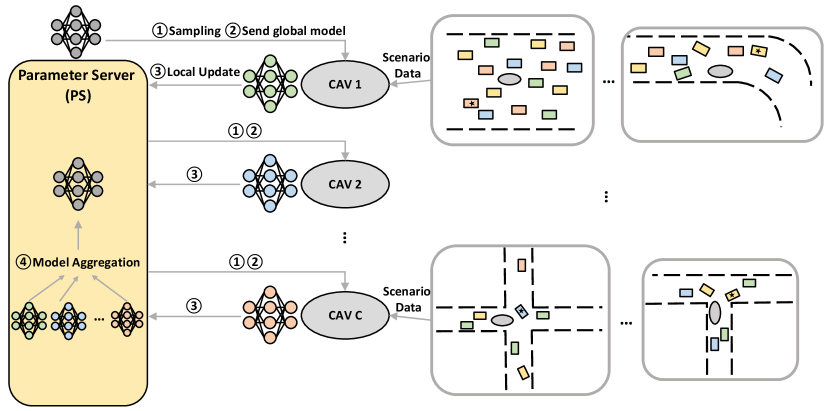
(a) The Framework of FLTP

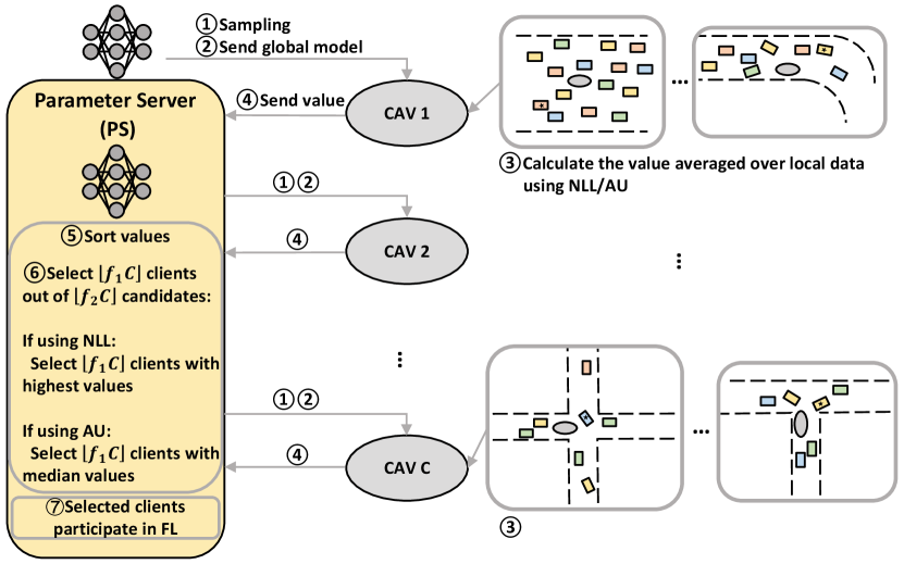
(b) The Framework of ALFLTP

Figure 1: Frameworks of FLTP and ALFLTP. Each gray oval represents a client (i.e., an ego vehicle) in FL. Each client collects its local driving scenario data using its sensors and cameras, does local updates, and communicates model weights with the central server. For each scenario, the ego vehicle aims to predict the future trajectory of the target vehicle (starred) based on past trajectories of agents in the scenario and map information. In ALFLTP, clients are actively selected for computation of each round based on values of candidate clients measured by NLL or AU. Specifically, if we use NLL as the metric, clients with $m$ highest values are selected, while for using AU as the metric, clients with $m$ median values are selected.

As shown in Fig.1(a), a driving scenario data (i.e. a data sample) can be described by a triple $S=(X,Y,\mathcal{M})$, where $X$ and $Y$ are the collections of observed and future trajectories of the involved agents (an agent can be a vehicle or a pedestrian), and $\mathcal{M}$ is the map information. Let $m$ denote the number of agents in the scenario, then $X$ and $Y$ can be expressed as $X=\{x_{1},...,x_{m}$} and $Y=\{y_{1},...,y_{m}$}, where $x_{i}\in\mathbb{R}^{2\times T_{obs}}$ and $y_{i}\in\mathbb{R}^{2\times T_{pre}}$ are the two-dimensional observed and future trajectory coordinates of agent $i$, with lengths $T_{obs}$ and $T_{pre}$, respectively. In particular, for any given scenario $S$, there is one target agent, denoted by $i^{*}$, among the $m$ agents which the ego vehicle is most interested in. In each scenario, the ego vehicle aims to predict the future trajectory of the target vehicle using $X$ and $\mathcal{M}$.

The system contains a server and $C$ autonomous vehicles, each of which can collect its driving scenario data using Lidar sensors and cameras to record the trajectories of all neighboring vehicles. We refer to each autonomous vehicle as one ego vehicle, which serves as one client in our FL framework. Each client $c\in\mathcal{C}\triangleq\{1,\cdots,C\}$ has a local dataset of size $K_{c}$, denoted as $\mathcal{D}_{c}=\{S^{1},S^{2},...,S^{K_{c}}\}$. Let $m_{c}^{k}$ be the number of agents in the $k$-th sample of client $c$. Let $K=\sum\limits_{c=1}^{C}K_{c}$ denote the total number of samples.

3.2 HiVT: Hierarchical Vector Transformer

Hierarchical Vector Transformer (HiVT) is a centralized, lightweight, and graph-based motion prediction model [6]. Towards scalability in the number of agents in the scene, HiVT decomposes the problem into local context extraction and global interaction modeling. HiVT achieves the state-of-the-art performance on the Argoverse motion forecasting benchmark. In this paper, we focus on training HiVT but under the FL framework. Different from the centralized HiVT, the local model updates at each client is done with respect to its local objective only.

Loss Function: As HiVT makes prediction for all agents in a scenario in one single forward pass, prediction results of all agents will be used in the training loss. Nevertheless, in the inference stage only the prediction result of the target agent is evaluated. Similarly, in Section 3.4, we do value calculation on the target agent only per driving scenario.

HiVT uses the Laplace mixture probability density function as part of its loss function with $\hat{\mu}_{i,t,f}\in\mathbb{R}^{2}$ and $\hat{b}_{i,t,f}\in\mathbb{R}^{2}$, respectively, denoting the estimated location and scale parameters for each agent $i\in\{1,...,m\}$ and each mixture component $f\in\{1,...,F\}$ at each prediction time step $t\in\{1,...,T_{pre}\}$. For any fixed $i$ and $t$, the two estimates $\hat{\mu}_{i,t,f}$ and $\hat{b}_{i,t,f}$ are interpreted as trajectory prediction and corresponding uncertainty, respectively, of the $f$-th predicted trajectory. The HiVT decoder also outputs predicted coefficients of the mixture model $\hat{P}_{i,f}\in\left[0,1\right]$ for each agent $i\in\{1,...,m\}$ and each mixture component $f\in\{1,...,F\}$.

HiVT only optimizes the best mode of $F$ trajectories. Specifically, the best trajectory for the $i$th agent is determined by the following equation:

$$f_{best_{i}}=\underset{f\in\{1,...,F\}}{\arg\min}\sum\limits_{t=1}^{T_{pre}}\|y_{i,t}-\hat{\mu}_{i,t,f}\|_{2}.$$ (1)

The regression loss is the negative log-likelihood (NLL) of the Laplace distribution, which is shown as follows:

$$L_{reg}=\frac{1}{m}\frac{1}{T_{pre}}\sum\limits_{i=1}^{m}\sum\limits_{t=1}^{T_{pre}}\left[\log(2\hat{b}_{i,t,f_{best_{i}}})+\frac{{\|y_{i,t}-\hat{\mu}_{i,t,f_{best_{i}}}\|}_{1}}{\hat{b}_{i,t,f_{best_{i}}}}\right]$$ (2)

The classification loss $L_{cls}$ is the cross entropy loss for optimizing mixture coefficients, which is shown as follows:

$$L_{cls}=\frac{1}{m}\sum\limits_{i=1}^{m}\sum\limits_{f=1}^{F}-P_{i,f}\log\hat{P}_{i,f}$$ (3)

with

$$P_{i,f}=\frac{\exp(-\sum\limits_{t=1}^{T_{pre}}\|\hat{\mu}_{i,t,f}-y_{i,t}\|_{2})}{\sum\limits_{j=1}^{F}{\exp(-\sum\limits_{t=1}^{T_{pre}}\|\hat{\mu}_{i,t,j}-y_{i,t}\|_{2})}}$$

Then the final loss for scenario $S$ with model weight $w$ is:

$$L(S,w)=L_{reg}+L_{cls}.$$ (4)

3.3 Federated Learning Based Trajectory Prediction (FLTP)

The loss function in Section 3.2 is defined for one driving scenario data. In FL, as client can only get access to its local data, then the local objective is defined as:

$$F_{c}(\mathcal{D}_{c},w)=\frac{1}{K_{c}}\sum\limits_{S\in\mathcal{D}_{c}}L(S,w)$$ (5)

We formally describe our FLTP in Algorithm 1. It follows the general server-client interaction of FedAvg [24]. Departing from the standard FedAvg, instead of stochastic gradient descent, we use AdamW as the local optimizer.

Specifically, in each global iteration:

• The parameter server first randomly chooses $\lfloor f_{1}C\rfloor$ clients according to the probability vector $[K_{1}/K,\cdots,K_{C}/K]$ without replacement, where $f_{1}\in(0,1]$ is the client sampling rate given as algorithm input. For example, let $C=3$, $f_{1}=\frac{2}{3}$, $K_{1}=1,K_{2}=2$, and $K_{3}=7$. The probability that client $1$ is chosen is $0.1+0.2\times\frac{0.1}{0.8}+0.7\times\frac{0.1}{0.3}$.

• Then the parameter server sends the current model $w_{r}$ to each of the chosen client $\mathcal{L}_{r}$ to get further improvement on their local data.

• In parallel, each of the chosen client run AdamW with respect to Eq.(5) with the specified minibatch size $B$ for $E$ epochs on local dataset. Concretely, in the ClientUpdate function, $\theta$ and $\Sigma$ are the weighted cumulative first and second moments, respectively, of the mini-batch gradients observed so far with $\beta_{1},\beta_{2}\in(0,1)$ as the momentum parameters. Depending on the minibatch size $B$, for the first few iterations in the inner for-loop, the smallest eigenvalues of $\hat{\Sigma}$ could be either zero or extermely small – resulting in significant fluctuation of $w$. Hence, $\epsilon>0$ is used to smooth the updates.

• Finally, upon reception of the local updates $w_{r+1}^{c}$, the parameter servers aggregates those models accordingly to their relative local data volume to obtain $w_{r+1}$.

It is worth noting that the algorithm can be improved via using global stepsize. We leave this direction to future work.

Algorithm 1 FLTP

0:  initial model $w_{0}$, number of clients $C$, client sampling rate $f_{1}\in(0,1]$, local data volume $\{K_{1},\cdots,K_{C}\}$, stepsize $\eta$, batch size $B$, number of epoch $E$, weight decay $\lambda$, momentum parameters $\beta_{1},\beta_{2}\in(0,1)$, smooth parameter $\epsilon$;

0:  $w_{R}$;

1:  Initialization: $w\leftarrow w_{0}$;

2:  for each round $r=1$ to $R$ do

3:     Randomly sample $\lfloor f_{1}C\rfloor$ clients according to the probability vector $[K_{1}/K,\cdots,K_{C}/K]$ without replacement. Let $\mathcal{L}_{r}$ denote the resulting set of clients;

4:     Send $w_{r-1}$ to each of the chosen client in $\mathcal{L}_{r}$;

5:     for each client $c\in\mathcal{L}_{r}$ in parallel do

6:        $w_{r}^{c}\leftarrow$ ClientUpdate$(w_{r},\eta,B,E,\beta_{1},\beta_{2},\epsilon)$;

7:     end for

8:     $w_{r}\leftarrow\sum\limits_{c\in\mathcal{L}_{r}}\frac{K_{c}}{\tilde{K}_{r}}w_{r}^{c}$, where $\tilde{K}_{r}\triangleq\sum\limits_{c\in\mathcal{L}_{r}}K_{c}$;

9:  end for

10:  return  $w_{R}$;

11:  ClientUpdate$(w,\eta,B,E,\beta_{1},\beta_{2},\epsilon)$

12:  Initialization: first moment $\theta\leftarrow 0$, second moment $\Sigma\leftarrow 0$, counter $t\leftarrow 0$;

13:  for each local epoch $i=1,\cdots,E$ do

14:     $\mathcal{B}_{c}\leftarrow$ divide $\mathcal{D}_{c}$ into batches with batch size $B$

15:     for each batch $b\in\mathcal{B}_{c}$ do

16:        $t\leftarrow t+1$

17:        $g=\nabla F_{c}(b,w)$

18:        $w\leftarrow w-\eta\lambda g$

19:        $\theta\leftarrow\beta_{1}\theta+(1-\beta_{1})g$, $\Sigma\leftarrow\beta_{2}\Sigma+(1-\beta_{2})gg^{\top}$

20:        $\hat{\theta}\leftarrow\frac{\theta}{1-\beta_{1}^{t}}$, $\hat{\Sigma}\leftarrow\frac{\Sigma}{1-\beta_{2}^{t}}$

21:        $w\leftarrow w-\eta\left(\hat{\Sigma}^{1/2}+\epsilon I\right)^{-1}\hat{\theta}$

22:     end for

23:  end for

24:  return  $w$

3.4 Active Learning-boosted FLTP (ALFLTP)

We use active learning to carefully select the clients to participate in each iteration. Departing from existing literature [36], instead of directly using the whole loss function as the metric, we consider two types of uncertainty-aware client selection metrics: negative log-likelihood (NLL) and aleatoric uncertainty (AU).

In our Algorithm 2, each client has a value variable $v_{i}$. In each round $r$ (where $r>2$), the parameter server samples the clients twice. It first randomly chooses $\lfloor f_{2}C\rfloor$ clients as it does in Algorithm 1. Each of the chosen clients in $\mathcal{Q}_{r}$ updates its local value $v$ according to

$$G_{c}(\mathcal{D}_{c},w)=\frac{1}{K_{c}}\sum\limits_{S\in\mathcal{D}_{c}}G(S,w)$$

where

$$G(S,w)=\begin{cases}\frac{1}{T_{pre}}\sum\limits_{t=1}^{T_{pre}}&\left[\log(2\hat{b}_{i^{*},t,f_{best_{i^{*}}}})+\frac{{\|y_{i,t}-\hat{\mu}_{i^{*},t,f_{best_{i^{*}}}}\|}_{1}}{\hat{b}_{i^{*},t,f_{best_{i^{*}}}}}\right]\qquad\qquad\text{if }NLL\\ \frac{1}{T_{pre}}\sum\limits_{t=1}^{T_{pre}}&\hat{b}_{i^{*},t,f_{best_{i^{*}}}}\qquad\qquad\text{if }AU\\ \end{cases}$$

where $\hat{\mu}_{i^{*},t,f_{best_{i^{*}}}}$ denotes prediction location of the target agent at time step $t$ from the best mode of $F$ trajectories and $\hat{b}_{i^{*},t,f_{best_{i^{*}}}}$ denotes the corresponding aleatoric uncertainty. All clients that are not contained in $\mathcal{Q}_{r}$ reset their values $v_{i}=0$. If NLL is used as the selection metric, then the parameter server chooses the set $\mathcal{L}_{r}$ to be the $\lfloor f_{1}C\rfloor$ clients with highest $v_{i}$; If AU is used as the metric, then the parameter server chooses $\mathcal{L}_{r}$ to contains the $\lfloor f_{1}C\rfloor$ whose values $v_{i}$ are closest to their median. When $r=1$ (i.e., lines 2-6 in Algorithm 2), as there is no global model from the last round for value calculation, client selection method is similar to that in FLTP.

Algorithm 2 ALFLTP

0:  initial model $w_{0}$, stepsize $\eta$, number of epoch $E$, client sampling rate $f_{1}\in(0,1]$, candidate sampling rate $f_{2}\in(0,1]$, local data volume $\{K_{1},\cdots,K_{C}\}$, weight decay $\lambda$, momentum parameters $\beta_{1},\beta_{2}\in(0,1)$, smooth parameter $\epsilon$;

0:  $w_{R}$

1:  Initialization $w\leftarrow w_{0}$

2:  The PS randomly samples $\lfloor f_{1}C\rfloor$ clients according to the probability vector $[K_{1}/K,\cdots,K_{C}/K]$ without replacement. Let $\mathcal{L}_{r}$ denote the resulting set of clients;

3:  for each client $c\in{\mathcal{L}}_{1}$ in parallel do

4:     $w_{1}^{c}\leftarrow$ ClientUpdate$(w,\eta,B,E,\beta_{1},\beta_{2},\epsilon)$

5:  end for

6:  $w_{1}\leftarrow\sum\limits_{c\in\mathcal{L}_{1}}\frac{K_{c}}{\tilde{K}_{1}}w_{1}^{c}$, where $\tilde{K}_{1}\triangleq\sum\limits_{c\in\mathcal{L}_{1}}K_{c}$

7:  for each round $r=2$ to $R$ do

8:     The PS selects $\lfloor f_{2}C\rfloor$ clients randomly as in line 2. Let $\mathcal{Q}_{r}$ denote the resulting client set;

9:     The PS broadcasts $w_{r-1}$ to each client in $\mathcal{Q}_{r}$;

10:     for each client $c$ in parallel do

11:        if $c\in\mathcal{Q}_{r}$ then

12:           $v_{c}\leftarrow G_{c}({\mathcal{D}_{c}},w_{r-1})$;

13:        else

14:           $v_{c}\leftarrow 0$

15:        end ifReports $v_{c}$ to the PS;

16:     end for

17:     The PS sorts $\{v_{c}\}_{c\in\mathcal{C}}$ 

18:     if u = NLL then

19:        The PS selects $\lfloor f_{1}C\rfloor$ clients with highest values $v_{i}$, denoting the resulting set as $\mathcal{L}_{r}$;

20:     else

21:        The PS selects $\lfloor f_{1}C\rfloor$ clients with values that closest to the median values $v_{i}$, denoting the resulting set as $\mathcal{L}_{r}$;

22:     end if

23:     for each client $c\in{\mathcal{L}}_{r}$ in parallel do

24:        $w_{r}^{c}\leftarrow$ ClientUpdate$(w,\eta,B,E,\beta_{1},\beta_{2},\epsilon)$

25:     end for

26:     $w_{r}\leftarrow\sum\limits_{c\in\mathcal{L}_{r}}\frac{K_{c}}{\tilde{K}_{r}}w_{r-1}^{c}$, where $\tilde{K}_{r}\triangleq\sum\limits_{c\in\mathcal{L}_{r}}K_{c}$.

27:  end for

NLL as a selection metric

We choose NLL as one selction metric for the following two reasons: Since NLL is incorporated as part of the loss function, a client has a higher NLL if the global model is not sufficiently trained with respect to its local data. As the local data is non-iid covering different driving scenarios, by selecting clients with higher NLL, the global model in FL is encouraged to do more local training on clients with more difficult data.

AU as a selection metric

This metric is inspired by [38], where incremental active learning is adopted for human trajectory prediction to evaluate candidate data samples and then select more valuable samples. Specifically, both noisy and redundant trajectory candidate data samples are removed and the model trained on filtered data samples achieves better performance. In our ALFLTP, we exploit aleatoric uncertainty to measure the degree of data noise. High aleatoric uncertainty means data are very noisy, while low aleatoric uncertainty means data are easy and the model is certain about them. As a result, we prefer clients with median aleatoric uncertainty, as data on these clients are both representative and less noisy.

Relaxing full client participation in updating $v$. For ease of exposition, in lines 10-15 of Algorithm 2, we let every client participate in updating $v_{c}$. In practice, it suffices to have the clients in $\mathcal{Q}_{r}$ do the value updates only. Since the value update does not rely on any previous value of $v_{c}$, the updated values are only used in the sorting at the PS, and the PS knows the $\mathcal{Q}_{r}$, the PS can treat $v_{c}=0$ for all $c\notin\mathcal{Q}_{r}$.

4 Experiments

4.1 Experimental Setup

Dataset: We use Argoverse Motion Forecasting v1.1 dataset for training and evaluation. In order to simulate distributed trajectory data for federated learning, we distribute the training set to 100 clients based on the city label of each data sample (driving scenario), where 95521 samples are from Pittsburgh and 110421 samples are from Miami. More specifically, the samples from the two cites, are evenly distributed to 50 clients, with each client denoting an autonomous vehicle that can collect and process traffic data in its area. The validation set contains 39472 samples. All training and validation scenarios consist of trajectories of 5 seconds sampled at 10 Hz and map information. The Argoverse Motion Forecasting challenge is to predict future trajectories of 3 seconds of focal agents with past trajectories of 2 seconds as inputs.

Model and Training Parameters: We use HiVT [6] with 64 hidden dimensions as our trajectory prediction model, which is a light-weight transformer based model. We use similar parameter settings for local HiVT models in FLTP and ALFLTP as the centralized HiVT. Specifically, for each local model in FLTP, learning rate $\eta$, weight decay, dropout rate, local batchsize $B$, local epochs $E$ and local optimizer are set to be $5\times 10^{-4}$, $1\times 10^{-4}$, $0.1$, $32$, $4$ and AdamW. We train FLTP and ALFLTP for 250 rounds. Fraction of clients selected for communication in each round $f_{1}$ is set to be 0.1.

Evaluation Metrics: We use NLL, Minimum Average Displacement Error (minADE), Minimum Final Displacement Error (minFDE) and Miss Rate (MR) to evaluate model performance quantitatively. minADE measures the average L2 distance between the best predicted trajectory (the trajectory with the minimum error at the endpoint) and the ground truth. minFDE measures the endpoint L2 distance between the best predicted trajectory and the ground truth. MR measures the fraction of the number of scenarios where endpoint errors of all predicted trajectories are larger than 2 meters.

4.2 FLTP v.s. training on local data

We quantitatively compare the global model of FLTP and the local model of an arbitrarily chosen client when it does not participate in communication and only updates using its local data. Here we have chosen the client 0; selecting any other client would yield the same result. As is shown in Fig. 2 and Table 1, FLTP significantly outperforms the client without FL, demonstrating the effectiveness of FLTP exploiting multi-source traffic data though it does not explicitly access raw local data. Specifically, after about 50 rounds, the local model of client 0 begins to exhibit worse performance as the number of training rounds increases, indicating the local model without FL has poor generalization.

Figure 2: Round-wise comparison between FLTP and the local model of client 0 without FL. Fraction of clients selected for communication in each round $f_{1}$ is set to be 0.1.

Figure 3: Round-wise comparison between FLTP and ALFLTP-NLL

Figure 4: Round-wise comparison between FLTP and ALFLTP-AU

Model	Round	NLL($\downarrow$)	minADE($\downarrow$)	minFDE($\downarrow$)	MR($\downarrow$)
Centralized HiVT [6]	-	0.467	0.685	1.028	0.104
Client 0 w/o FL	50	0.897	0.992	1.732	0.207
FLTP	50	0.629	0.818	1.318	0.140
ALFLTP-NLL($f_{2}$=0.15)	50	0.634	0.821	1.318	0.138
ALFLTP-NLL($f_{2}$=0.30)	50	0.636	0.816	1.319	0.141
ALFLTP-AU($f_{2}$=0.15)	50	0.629	0.819	1.325	0.139
ALFLTP-AU($f_{2}$=0.30)	50	0.625	0.813	1.318	0.141
Client 0 w/o FL	150	1.098	1.026	1.822	0.229
FLTP	150	0.551	0.751	1.170	0.123
ALFLTP-NLL($f_{2}$=0.15)	150	0.552	0.750	1.179	0.122
ALFLTP-NLL($f_{2}$=0.30)	150	0.564	0.753	1.170	0.120
ALFLTP-AU($f_{2}$=0.15)	150	0.555	0.753	1.177	0.119
ALFLTP-AU($f_{2}$=0.30)	150	0.554	0.752	1.170	0.119
Client 0 w/o FL	250	1.259	1.059	1.896	0.245
FLTP	250	0.527	0.730	1.122	0.114
ALFLTP-NLL($f_{2}$=0.15)	250	0.532	0.732	1.139	0.116
ALFLTP-NLL($f_{2}$=0.30)	250	0.536	0.733	1.126	0.114
ALFLTP-AU($f_{2}$=0.15)	250	0.531	0.731	1.131	0.115
ALFLTP-AU($f_{2}$=0.30)	250	0.526	0.729	1.126	0.114

Table 1: Performance on Argoverse Validation Set. Fraction of clients selected for communication in each round $f_{1}$ is set to be 0.1.

4.3 Comparison between FLTP and ALFLTP

In this section, ALFLTP frameworks using two active client selection metrics together with different degrees of bias are compared with FLTP. From Fig. 3 and Fig. 4 we can see that:

• Convergence speed of training loss: Regression loss of both ALFLTP-NLL and ALFLTP-AU with $f_{2}=0.30$ converge faster than with $f_{2}=0.15$ and FLTP.

• Round-wise validation performance: ALFLTP-NLL and ALFLTP-AU with both $f_{2}=0.15$ and $f_{2}=0.30$ perform better than FLTP in terms of MR. As MR measures the fraction of scenarios with endpoint errors larger than 2 meters, lower MR demonstrates that ALFLTP-NLL and ALFLTP-AU are more robust to various traffic scenarios in the inference stage.

• Impact of biased selection-NLL: After around 100 rounds, FLTP surpasses the performance of ALFLTP-NLL with both $f_{2}=0.15$ and $f_{2}=0.30$ in terms of minADE and minFDE due to biased selection. Notably, ALFLTP-NLL with $f_{2}=0.30$ performs worse than it with $f_{2}=0.15$, because the former introduces more bias.

• Impact of biased selection-AU: Compared to ALFLTP-NLL with $f_{2}=0.15$ and $f_{2}=0.30$ and ALFLTP-AU with $f_{2}=0.15$, ALFLTP-AU with $f_{2}=0.30$ achieves comparable minADE and minFDE to FLTP while does better in terms of MR in most rounds, indicating that a larger $f_{2}$ helps ALFLTP-AU to find clients with more representative data.

Table 1 shows detailed global model performance of specific rounds, where we can see that:

• In the 50th round, ALFLTP-AU with $f_{2}=0.30$ outperforms other frameworks in NLL, minADE and minFDE.

• In the 150th round, ALFLTP-AU with $f_{2}=0.15$ and $f_{2}=0.30$ outperform other frameworks in terms of minADE.

• In the 250th round, where global models finish training, ALFLTP-AU with $f_{2}=0.30$ outperforms other frameworks in terms of NLL, minADE and MR.

• Although FLTP based HiVT models in the 250th round perform slightly worse than the centralized HiVT, it protects the privacy of the human-driven vehicles by avoiding the data exchange with the server.

In a word, ALFLTP-AU converges faster in regression loss and has better performance in terms of NLL, minADE and MR than FLTP in most rounds. Moreover, ALFLTP-AU shows better and more stable round-wise performance than ALFLTP-NLL.

5 Conclusion

In this paper, we propose a privacy-preserving and uncertainty-aware trajectory prediction framework for connected autonomous vehicles using federated learning with a uncertainty-aware global objective. We term this framework as FLTP, where we relax the requirement of collecting raw data of driving scenarios to form a large centralized dataset and let CAVs collect local traffic data and collaboratively train trajectory prediction models without explicit data exchange, thus preserving privacy of traffic participants. We further introduce Active Learning-boosted FLTP (ALFLTP) for client selection in FLTP, where we adopt two uncertainty-aware metrics, negative log-likelihood (NLL) and aleatoric uncertainty (AU) to actively select clients for partial client participation in FLTP. Experiments on Argoverse dataset demonstrate that FLTP significantly outperforms the model trained on local data. In addition, ALFLTP-AU has a faster convergence speed in training regression loss and performs better in terms of NLL, minADE and MR than FLTP in most rounds, and has more stable round-wise performance than ALFLTP-NLL.

References

- [1] Mayank Bansal, Alex Krizhevsky, and Abhijit Ogale. Chauffeurnet: Learning to drive by imitating the best and synthesizing the worst. arXiv preprint arXiv:1812.03079, 2018.
- [2] Henggang Cui, Vladan Radosavljevic, Fang-Chieh Chou, Tsung-Han Lin, Thi Nguyen, Tzu-Kuo Huang, Jeff Schneider, and Nemanja Djuric. Multimodal trajectory predictions for autonomous driving using deep convolutional networks. In 2019 International Conference on Robotics and Automation (ICRA), pages 2090–2096. IEEE, 2019.
- [3] Nemanja Djuric, Vladan Radosavljevic, Henggang Cui, Thi Nguyen, Fang-Chieh Chou, Tsung-Han Lin, Nitin Singh, and Jeff Schneider. Uncertainty-aware short-term motion prediction of traffic actors for autonomous driving. In Proceedings of the IEEE/CVF Winter Conference on Applications of Computer Vision, pages 2095–2104, 2020.
- [4] Ming Liang, Bin Yang, Rui Hu, Yun Chen, Renjie Liao, Song Feng, and Raquel Urtasun. Learning lane graph representations for motion forecasting. In Computer Vision–ECCV 2020: 16th European Conference, Glasgow, UK, August 23–28, 2020, Proceedings, Part II 16, pages 541–556. Springer, 2020.
- [5] Jiyang Gao, Chen Sun, Hang Zhao, Yi Shen, Dragomir Anguelov, Congcong Li, and Cordelia Schmid. Vectornet: Encoding hd maps and agent dynamics from vectorized representation. In Proceedings of the IEEE/CVF Conference on Computer Vision and Pattern Recognition, pages 11525–11533, 2020.
- [6] Zikang Zhou, Luyao Ye, Jianping Wang, Kui Wu, and Kejie Lu. Hivt: Hierarchical vector transformer for multi-agent motion prediction. In Proceedings of the IEEE/CVF Conference on Computer Vision and Pattern Recognition, pages 8823–8833, 2022.
- [7] Jiquan Ngiam, Benjamin Caine, Vijay Vasudevan, Zhengdong Zhang, Hao-Tien Lewis Chiang, Jeffrey Ling, Rebecca Roelofs, Alex Bewley, Chenxi Liu, Ashish Venugopal, et al. Scene transformer: A unified architecture for predicting multiple agent trajectories. arXiv preprint arXiv:2106.08417, 2021.
- [8] Junru Gu, Chen Sun, and Hang Zhao. Densetnt: End-to-end trajectory prediction from dense goal sets. In Proceedings of the IEEE/CVF International Conference on Computer Vision, pages 15303–15312, 2021.
- [9] Yicheng Liu, Jinghuai Zhang, Liangji Fang, Qinhong Jiang, and Bolei Zhou. Multimodal motion prediction with stacked transformers. In Proceedings of the IEEE/CVF Conference on Computer Vision and Pattern Recognition, pages 7577–7586, 2021.
- [10] Xinshuo Weng, Boris Ivanovic, Kris Kitani, and Marco Pavone. Whose track is it anyway? improving robustness to tracking errors with affinity-based trajectory prediction. In Proceedings of the IEEE/CVF Conference on Computer Vision and Pattern Recognition, pages 6573–6582, 2022.
- [11] Qingzhao Zhang, Shengtuo Hu, Jiachen Sun, Qi Alfred Chen, and Z Morley Mao. On adversarial robustness of trajectory prediction for autonomous vehicles. In Proceedings of the IEEE/CVF Conference on Computer Vision and Pattern Recognition, pages 15159–15168, 2022.
- [12] Mohammadhossein Bahari, Saeed Saadatnejad, Ahmad Rahimi, Mohammad Shaverdikondori, Amir Hossein Shahidzadeh, Seyed-Mohsen Moosavi-Dezfooli, and Alexandre Alahi. Vehicle trajectory prediction works, but not everywhere. In Proceedings of the IEEE/CVF Conference on Computer Vision and Pattern Recognition, pages 17123–17133, 2022.
- [13] Dorothy J Glancy. Privacy in autonomous vehicles. Santa Clara L. Rev., 52:1171, 2012.
- [14] Arendse Huld. How did didi run afoul of china’s cybersecurity regulators? understanding the us $1.2 billion fine, 2022.
- [15] Man Zhang, Bran Selic, Shaukat Ali, Tao Yue, Oscar Okariz, and Roland Norgren. Understanding uncertainty in cyber-physical systems: a conceptual model. In Modelling Foundations and Applications: 12th European Conference, ECMFA 2016, Held as Part of STAF 2016, Vienna, Austria, July 6-7, 2016, Proceedings 12, pages 247–264. Springer, 2016.
- [16] Hsu-kuang Chiu, Jie Li, Rareş Ambruş, and Jeannette Bohg. Probabilistic 3d multi-modal, multi-object tracking for autonomous driving. In 2021 IEEE International Conference on Robotics and Automation (ICRA), pages 14227–14233. IEEE, 2021.
- [17] Sanbao Su, Yiming Li, Sihong He, Songyang Han, Chen Feng, Caiwen Ding, and Fei Miao. Uncertainty quantification of collaborative detection for self-driving. arXiv preprint arXiv:2209.08162, 2022.
- [18] Bohan Tang, Yiqi Zhong, Ulrich Neumann, Gang Wang, Siheng Chen, and Ya Zhang. Collaborative uncertainty in multi-agent trajectory forecasting. Advances in Neural Information Processing Systems, 34:6328–6340, 2021.
- [19] Guopeng Li, Zirui LI, Victor Knoop, and Hans van Lint. Uqnet: Quantifying uncertainty in trajectory prediction by a non-parametric and generalizable approach. Available at SSRN 4241523, 2022.
- [20] Xiaolin Tang, Kai Yang, Hong Wang, Jiahang Wu, Yechen Qin, Wenhao Yu, and Dongpu Cao. Prediction-uncertainty-aware decision-making for autonomous vehicles. IEEE Transactions on Intelligent Vehicles, 7(4):849–862, 2022.
- [21] Nachiket Deo and Mohan M Trivedi. Convolutional social pooling for vehicle trajectory prediction. In Proceedings of the IEEE conference on computer vision and pattern recognition workshops, pages 1468–1476, 2018.
- [22] Yarin Gal and Zoubin Ghahramani. Dropout as a bayesian approximation: Representing model uncertainty in deep learning. In international conference on machine learning, pages 1050–1059. PMLR, 2016.
- [23] Balaji Lakshminarayanan, Alexander Pritzel, and Charles Blundell. Simple and scalable predictive uncertainty estimation using deep ensembles. Advances in neural information processing systems, 30, 2017.
- [24] Brendan McMahan, Eider Moore, Daniel Ramage, Seth Hampson, and Blaise Aguera y Arcas. Communication-efficient learning of deep networks from decentralized data. In Artificial intelligence and statistics, pages 1273–1282. PMLR, 2017.
- [25] Peter Kairouz, H Brendan McMahan, Brendan Avent, Aurélien Bellet, Mehdi Bennis, Arjun Nitin Bhagoji, Kallista Bonawitz, Zachary Charles, Graham Cormode, Rachel Cummings, et al. Advances and open problems in federated learning. Foundations and Trends® in Machine Learning, 14(1–2):1–210, 2021.
- [26] Haoran Song, Wenchao Ding, Yuxuan Chen, Shaojie Shen, Michael Yu Wang, and Qifeng Chen. Pip: Planning-informed trajectory prediction for autonomous driving. In Computer Vision–ECCV 2020: 16th European Conference, Glasgow, UK, August 23–28, 2020, Proceedings, Part XXI 16, pages 598–614. Springer, 2020.
- [27] Ye Yuan, Xinshuo Weng, Yanglan Ou, and Kris M Kitani. Agentformer: Agent-aware transformers for socio-temporal multi-agent forecasting. In Proceedings of the IEEE/CVF International Conference on Computer Vision, pages 9813–9823, 2021.
- [28] Xin Li, Xiaowen Ying, and Mooi Choo Chuah. Grip: Graph-based interaction-aware trajectory prediction. In 2019 IEEE Intelligent Transportation Systems Conference (ITSC), pages 3960–3966. IEEE, 2019.
- [29] Hyeongseok Jeon, Junwon Choi, and Dongsuk Kum. Scale-net: Scalable vehicle trajectory prediction network under random number of interacting vehicles via edge-enhanced graph convolutional neural network. In 2020 IEEE/RSJ International Conference on Intelligent Robots and Systems (IROS), pages 2095–2102. IEEE, 2020.
- [30] Yuning Chai, Benjamin Sapp, Mayank Bansal, and Dragomir Anguelov. Multipath: Multiple probabilistic anchor trajectory hypotheses for behavior prediction. arXiv preprint arXiv:1910.05449, 2019.
- [31] Tung Phan-Minh, Elena Corina Grigore, Freddy A Boulton, Oscar Beijbom, and Eric M Wolff. Covernet: Multimodal behavior prediction using trajectory sets. In Proceedings of the IEEE/CVF Conference on Computer Vision and Pattern Recognition, pages 14074–14083, 2020.
- [32] Hang Zhao, Jiyang Gao, Tian Lan, Chen Sun, Ben Sapp, Balakrishnan Varadarajan, Yue Shen, Yi Shen, Yuning Chai, Cordelia Schmid, et al. Tnt: Target-driven trajectory prediction. In Conference on Robot Learning, pages 895–904. PMLR, 2021.
- [33] Nathalie Majcherczyk, Nishan Srishankar, and Carlo Pinciroli. Flow-fl: Data-driven federated learning for spatio-temporal predictions in multi-robot systems. In 2021 IEEE International Conference on Robotics and Automation (ICRA), pages 8836–8842. IEEE, 2021.
- [34] Chunnan Wang, Xiang Chen, Junzhe Wang, and Hongzhi Wang. Atpfl: Automatic trajectory prediction model design under federated learning framework. In Proceedings of the IEEE/CVF Conference on Computer Vision and Pattern Recognition, pages 6563–6572, 2022.
- [35] Jack Goetz, Kshitiz Malik, Duc Bui, Seungwhan Moon, Honglei Liu, and Anuj Kumar. Active federated learning. arXiv preprint arXiv:1909.12641, 2019.
- [36] Yae Jee Cho, Jianyu Wang, and Gauri Joshi. Client selection in federated learning: Convergence analysis and power-of-choice selection strategies. arXiv preprint arXiv:2010.01243, 2020.
- [37] Pengfei Li, Yunfeng Zhao, Liandong Chen, Kai Cheng, Chuyue Xie, Xiaofei Wang, and Qinghua Hu. Uncertainty measured active client selection for federated learning in smart grid. In 2022 IEEE International Conference on Smart Internet of Things (SmartIoT), pages 148–153. IEEE, 2022.
- [38] Yi Xi, Dongchun Ren, Mingxia Li, Yuehai Chen, Mingyu Fan, and Huaxia Xia. Robust trajectory prediction of multiple interacting pedestrians via incremental active learning. In Neural Information Processing: 28th International Conference, ICONIP 2021, Sanur, Bali, Indonesia, December 8–12, 2021, Proceedings, Part V 28, pages 141–150. Springer, 2021.