QuickSRNet: Plain Single-Image Super-Resolution Architecture
for Faster Inference on Mobile Platforms

Abstract

In this work, we present QuickSRNet, an efficient super-resolution architecture for real-time applications on mobile platforms. Super-resolution clarifies, sharpens, and upscales an image to higher resolution. Applications such as gaming and video playback along with the ever-improving display capabilities of TVs, smartphones, and VR headsets are driving the need for efficient upscaling solutions. While existing deep learning-based super-resolution approaches achieve impressive results in terms of visual quality, enabling real-time DL-based super-resolution on mobile devices with compute, thermal, and power constraints is challenging. To address these challenges, we propose QuickSRNet, a simple yet effective architecture that provides better accuracy-to-latency trade-offs than existing neural architectures for single-image super-resolution. We present training tricks to speed up existing residual-based super-resolution architectures while maintaining robustness to quantization. Our proposed architecture produces 1080p outputs via 2$\times$ upscaling in 2.2 ms on a modern smartphone, making it ideal for high-fps real-time applications.

1 Introduction

Single-image super-resolution (SR) refers to a family of techniques that recover a high-resolution (HR) image $I_{HR}$ from its low-resolution (LR) counterpart $I_{LR}$. In recent years, deep learning (DL) based approaches have become increasingly popular in the field [10, 11, 35, 20, 28, 24, 27, 6, 34], producing impressive results compared to interpolation-based techniques and hand-engineered heuristics (see Fig. 2). However, most existing DL-based super-resolution solutions are computationally intensive and not suitable for real-time applications requiring interactive frame rates, such as mobile gaming. While DL-based super-resolution has been successfully applied to gaming on high-end GPU desktops [26, 7], neural approaches are still impractical for mobile gaming due to their high latency and computational costs. For example, a DL-based architecture such as EDSR [24] takes $75$ ms to upscale a $540$p image to $1080$p on a state-of-the-art mobile AI accelerator. This has driven the need for efficient DL-based super-resolution solutions [2, 13, 5, 38, 12] that can be used in real-time applications such as video gaming, where responsiveness and higher frame rates are essential.

Figure 1: Accuracy-to-latency trade-offs of QuickSRNet (ours) against existing SISR architectures. We report accuracy after 8-bit quantization and measure latency on a state-of-the-art mobile AI accelerator.

(a) LR

(b) Interpolation

(c) Algorithmic approach

(d) ML-based approach

Figure 2: Side-by-side comparison of various upscaling approaches: (a) Low-resolution, (b) Bicubic interpolation, (c) Non-ML baseline: FSR1.0 [14], (d) ML baseline: EDSR [24].

In this work, rather than trying to achieve the state-of-the-art PSNR or SSIM scores on standard super-resolution benchmarks, we aim to develop efficient architectures that are suitable for high-fps real-time applications on mobile devices. To this end, we propose QuickSRNet, a simple single-image super-resolution neural network that obtains better accuracy-to-latency trade-offs than existing efficient SR architectures. In particular, we make the following key contributions:

• We streamline the network architecture, reduce the impact of residual connection removal, and ultimately demonstrate the effectiveness of simpler designs in achieving high levels of accuracy and on-device performance.

• We compare a wide variety of architectures in terms of on-device latency, measured on a device with Snapdragon^® 8 Gen 1 Mobile Platform, instead of FLOPS count, which is not a reliable indicator of on-device performance [18].

• We measure accuracy after 8-bit quantization, a necessary step for better efficiency on mobile platforms, and describe architectural tricks that improve robustness to quantization.

• We apply our proposed architecture to a real-world use-case (video gaming) and compare its visual quality against that of a well-known industrial non-ML based approach (AMD’s FidelityFX Super Resolution (FSR1.0) algorithm [14]).

• We describe an approach to perform $1.5\times$ upscaling, a setting that is occasionally used in gaming and XR use-cases but not trivially supported by SR architectures whose upscaling step is based on a sub-pixel convolution [35].

Figure 3: QuickSRNet architecture. We use the convention QuickSRNet-f$X$-m$Y$ to refer to the architecture variant that has $Y$ intermediate conv layers and $X$ feature channels. We use dotted lines to illustrate that the conv layers are initialized using an identity initialization scheme. In practice, these skip connections are incorporated into the weights of the corresponding conv module. $p$ and $ri$ stand for “partial” and “repeat-interleaving” respectively (see Sec. 3.2 for more details).

2 Related work

Several efficient SR architectures have been proposed recently. Overall, these architectures share many characteristics with the earlier work by [11] and [35] on FSRCNN and ESPCN respectively: they are usually fully convolutional, use a relatively small number of layers and channels, all layers run at the input resolution and the final output is mapped to higher resolution using a subpixel convolution. Compared to these baselines, more recent approaches have incorporated the following changes:

XLSR

[2] uses grouped convolutions to reduce the computational footprint of the architecture and “clipped” ReLU activations to improve robustness to quantization.

ABPN

[13] employs a VGG-like convnet [37] (i.e. consisting of only $3\times 3$ Conv-ReLU blocks) with an “anchor-based” input-to-output residual connection. This “anchor-based” connection adds a channel-wise nearest-neighbor upscaled version of the input to the output before the final depth-to-space operation. We confirmed that this channel-wise implementation runs faster on our profiling device than the more common approach of adding the spatially-upsampled input directly to the output. Thus, we follow the same strategy to implement input-to-output residual connections in all our experiments.

SESR

[5] leverages linear over-parameterized residual modules which are collapsed into regular convolutions during inference for improved on-device performance. Other modifications include the use of long residual connections.

RepSR

[38] investigates training VGG-like super-resolution architectures. Like ABPN, their convnet is equipped with a nearest-neighbor upsampling-based input-to-output connection. Similar to SESR, they find that using over-parameterized networks during training can boost accuracy. They propose a training scheme for using Batch Normalization (BN) layers [22] without introducing artifacts in flat regions of the image, a typical side effect of BN when employed for super-resolution. At test time, the over-parameterized, BN-equipped network is collapsed into a simpler, more efficient network.

Residual learning for super-resolution

Many SR architectures utilize a long skip connection which adds an upscaled version of the input $U(I_{LR})$ directly to the output. Efficient architectures (like [13, 38]) will often implement $U$ as nearest-neighbour interpolation. During training, SR architectures equipped with this technique are implicitly optimized to produce a residual $R=I_{HR}-U(I_{LR})$. One benefit is that the network produces reasonable outputs right after initialization which stabilizes training. Additionally, the input-to-output connection makes the architecture significantly more robust to quantization, as discussed in the next section.

3 Methodology

This section contains a detailed description of QuickSRNet as well as implementation details. The process for developing our proposed SR architecture began with preliminary experiments, which we present in the next paragraph.

3.1 On the impact of removing the input-to-output residual connection

Architecture	PSNR (dB)		Latency (ms)
	FP16	INT8
ABPN	31.84 (baseline)	31.80 (baseline)	2.17 (baseline)
Res.-free ABPN	31.75 ($-$0.09)	31.50 ($-$0.30)	1.42 ($-$35%)
QSRNet-Med	31.82 ($-$0.02)	31.77 ($-$0.03)	1.42 ($-$35%)

Table 1: On the accuracy and latency impacts of removing the input-to-output residual connection from the ABPN architecture. We report PSNR numbers obtained on BSD100 via $2\times$ upscaling. Latency numbers were obtained on a device with Snapdragon 8 Gen 1 using an input resolution of $512\times 512$.

VGG-style architectures such as ABPN [13] or RepSR [38] are already well-optimized, so it is unclear how much faster they can be made on mobile AI accelerators. Instinctively, reducing the number of layers and channels, or replacing $3\times 3$ kernels with $1\times 1$ kernels, can improve speed at the cost of accuracy. Instead, our experiments investigate how to effectively remove the input-to-output residual connection without affecting accuracy.

As observed by [2, 13], long residual connections can have a large impact on the efficiency of super-resolution architectures, particularly on memory-limited platforms such as smartphones or VR headsets. To confirm this, we trained and profiled a residual-free ABPN variant and found that removing the input-to-output residual connection improves latency by $35\%$. However, this modification resulted in a marginally lower accuracy and more importantly, reduced robustness to quantization, as can be seen in Tab. 1. A similar trend is evident in the results of the Mobile AI 2022 Challenge [21], where the fastest approaches do not use input-to-output residual connections at the cost of accuracy. To address this, we propose QuickSRNet, a residual-free architecture which is robust to quantization.

3.2 QuickSRNet

HR

SESR-M7

ABPN

EDSR

Bicubic
empty

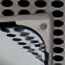
Ours-Small
(1.5$\times$ faster)

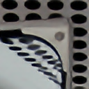
Ours-Medium
(1.3$\times$ faster)

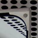
Ours-Large
(1.8$\times$ faster)

Figure 4: Visualization of 4× super-resolved images from Urban100 produced by our models and existing baselines. Our models match the quality of existing architectures while being significantly faster.

Our architecture, QuickSRNet, follows a VGG-like structure with no input-to-output residual connection (see Fig. 3). This architecture is denoted by $m$, the number of intermediate convolutional blocks, and $f$, the number of feature channels in those intermediate layers. To increase robustness to quantization, we use a residual learning-motivated initialization scheme along with clipped ReLU activations:

Identity initialization

We utilize an intuitive initialization technique where each intermediate convolutional layer simulates a localized skip connection:

$$y=W\circledast x+x$$ (1)

where $\circledast$ is the discrete convolution operator and $W$ refers to the kernel weights. In practice, we collapse the skip connection into the conv module: $y=(W+I)\circledast x=\hat{W}\circledast x$, where $\hat{W}$ are the modified weights after collapse and $I$ is the identity of discrete convolution operators. In this case, collapsing amounts to adding a diagonal of ones to the randomly initialized kernel sliced at the spatial center: $\forall i,W[i,i,c_{x},c_{y}]\mathrel{+}=1$ (with $c_{x}=c_{y}=1$ assuming a $3\times 3$ kernel). This approach is akin to identity initialization [16, 41, 3, 42] and related to the over-parameterized networks used in [39, 9, 5, 38], except we collapse before training, during initialization.

Equation 1 only works if $x$ and $y$ have the same dimensions and is therefore not directly applicable to the first and last layer of the architecture, as these layers respectively change the number of channels from $3$ to $f$ and $f$ to $3\times S^{2}$, where $S$ is the scaling factor. For these layers, we modify the initialization scheme as follows:

• Partial identity initialization: the $3$-channel input to the first convolutional module are added to the first $3$ output channels and the other $f-3$ output channels are left unchanged.

  $$y_{i}=\begin{cases}(W\circledast x)_{i}+x_{i},&\text{if }0\leq i<3\\ (W\circledast x)_{i},&\text{otherwise}\end{cases}$$ (2)

• Repeat-interleaving identity initialization: the first $3$ input channels to the final convolutional module are repeat-interleaved $S^{2}$ times and added to the output.

  $$y_{i}=(W\circledast x)_{i}+x_{round\left(\frac{i}{s^{2}}\right)}$$ (3)

Similar to Eq. 1, the skip connections described in Eqs. 2 and 3 are incorporated into the corresponding convolutional module by adding ones to the kernel weights at the appropriate location. Intuitively, this initialization technique makes the input image propagate well throughout the entire network. The repeat-interleaving scheme used to initialize the final layer mimics the nearest-neighbour upscaling typically performed in the input-to-output connection of existing residual architectures.

ReLU1

In addition to identity initialization, we found that clipping ReLU activations between $0$ and $1$ improves robustness to quantization. Compared to XLSR [2], we use ReLU1s throughout the entire network as opposed to just the final layer. Note that for this approach to work well with our id-initialized architecture, it is important to scale input pixels between $0$ and $1$ (centering around $0$ would cause roughly half the pixels propagated by the first id-initialized conv to be zeroed out).

Our experimental results (Sec. 4) show that combining identity initialization and ReLU1 activations significantly improve robustness to quantization.

FP16

FP16

FP16

FP16

INT8

INT8

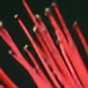
INT8

INT8

Figure 5: Visual comparison of 4$\times$ super-resolved images from DIV2K produced by QuickSRNet-Medium before and after quantization.

3.3 Implementation details

Baselines

We compare QuickSRNet against the following architectures: FSRCNN [11], ESPCN [35], XLSR [2], SESR [5], ABPN [13], ERFDN [27] and EDSR [24]. Note that, rather than reporting PSNR and SSIM scores from the original papers, we re-implemented, trained and quantized all existing baselines from scratch. As a result, all models shared most hyper-parameters (batch-size, losses, optimizer, etc.), including the data loading/augmentation pipeline. We did however tweak the learning rate for each architecture independently. In some cases, our re-implementation deviates slightly from the original architecture when it includes operations that are not supported on the device used for profiling. For example, we replaced the parametric ReLUs [17] used in SESR and FSRCNN to regular ReLUs. Despite these minor modifications, we were usually able to reproduce PSNR and SSIM scores reported in the original papers.

Training details

For most experiments, we train the models on the $800$ training images from the DIV2K dataset [1] and evaluate them on standard SR testsets: Set5 [4], Set14 [40], BSD100 [29], and Urban100 [19]. We preprocess input and target images by scaling RGB values between $0$ and $1$. For data augmentation, we use random cropping, flipping and rotation. The models are trained for 1 million iterations with a batch size of $32$. We use an L1 loss and the Adam optimizer [23] with hyper-parameters $\epsilon=10^{-8}$ and $\beta=(0.9,0.999)$. For the learning rate, we found that using an initial value of $5\times 10^{-4}$ and decaying it by a factor of $0.5$ every $200$K iterations is a strategy that works well for most architectures.

8-bit quantization

We use the AIMET library [36] to perform model quantization [32] and compute post-quantization accuracy metrics. Both weights and activations are quantized to 8-bit integers (W8A8 setup). We experimented with both Post-Training Quantization (PTQ) techniques and Quantization Aware Training (QAT). When we use QAT, we re-initialize the optimizer with a very small learning rate (usually $4\times 10^{-6}$).

On-device profiling

We profile the models on the Hexagon Processor of a device with Snapdragon 8 Gen 1 and report the average latency obtained on $100$ inputs of spatial resolution $512\times 512$. Before profiling, the model is converted from PyTorch [33] to ONNX. Please see the appendix for more details about the model conversion steps.

QuickSRNet specs	$\bm{2\times}$		$\bm{3\times}$		$\bm{4\times}$		Latency
	FP16	INT8	FP16	INT8	FP16	INT8	Measurements (ms)
f32 - m1	31.43	31.38	28.41	28.38	26.94	26.91	0.99 ($-$22%)
f32 - m2 (small)	31.61	31.58	28.57	28.55	27.07	27.06	1.14 ($-$35%)
f32 - m3	31.72	31.63	28.67	28.63	27.16	27.12	1.21 ($-$34%)
f32 - m5 (medium)	31.82	31.77	28.75	28.72	27.24	27.21	1.42 ($-$35%)
f32 - m7	31.88	31.81	28.81	28.76	27.30	27.27	1.74 ($-$30%)
f32 - m11	31.95	31.80	28.86	28.80	27.35	27.29	2.38 ($-$22%)
f64 - m11 (large)	32.08	31.97	28.98	28.93	27.47	27.43	7.63 (  $-$7%)

Table 2: PSNRs (dB) and latencies (ms) of various QuickSRNet configurations ($f$ : number of feature channels, $m$ : number of convolutional blocks in the network). We report PSNR numbers obtained before and after quantization. We also report latency measurements on a $512\times 512$ input, obtained on a device with Snapdragon 8 Gen 1, and gains introduced by not using an input-to-output residual connection.

Existing Models	$\bm{2\times}$		$\bm{3\times}$		$\bm{4\times}$		Latency
	FP16	INT8	FP16	INT8	FP16	INT8	Measurements (ms)
XLSR	31.62	31.32	28.59	28.31	27.09	26.82	1.59
ESPCN	31.37	30.19	28.35	27.86	26.87	26.44	1.83
SESR-M3	31.57	31.40	28.52	28.47	27.02	26.97	2.02
ABPN	31.80	31.74	28.73	28.70	27.22	27.20	2.09
SESR-M5	31.68	31.53	28.63	28.56	27.11	27.05	2.23
SESR-M7	31.76	31.67	28.68	28.61	27.16	27.07	2.33
SESR-M11	31.84	31.74	28.77	28.60	27.25	27.18	3.06
FSRCNN	31.50	31.22	28.49	28.32	26.99	26.89	3.45
SESR-XL	32.02	31.94	28.91	28.85	27.39	27.35	3.75
ERFDN	32.20	32.06	29.08	28.98	27.57	27.48	19.50
EDSR	32.21	32.08	29.04	28.89	27.61	27.53	37.95

Table 3: PSNRs (dB) and latencies (ms) of existing SISR solutions on BSD100. Please note that we re-implemented, trained, and quantized all architectures from scratch. Latency numbers were measured on a device with Snapdragon 8 Gen 1, using a $512\times 512$ input.

ABPN

QSRNet-Medium

Figure 6: Visual artifacts by ABPN vs QuickSRNet-Medium on $4\times$-upscaled images from Urban100. More examples can be found in the supplementary material.

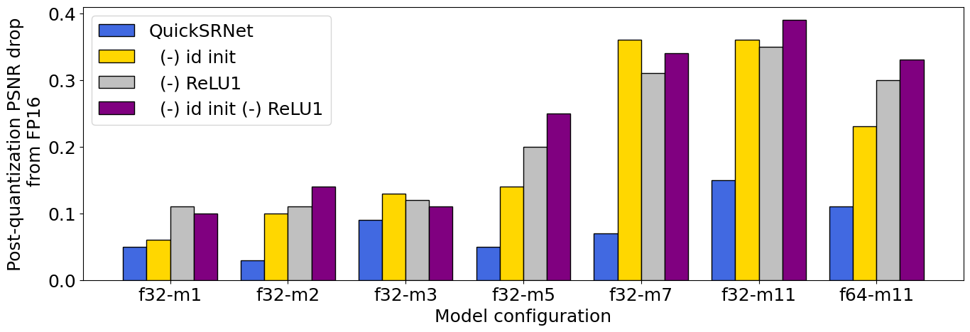
Figure 7: Ablation study comparing the post-quantization PSNR drop from FP16 when removing identity initialization and/or ReLU1 activations from the architecture design.

Specification	Post-training	No optimizations	QAT	Per-channel QAT	Per-channel Adaround
	FP16	INT8	INT8	INT8	INT8
QuickSRNet-Small	31.61	30.81 ($-$0.80)	31.34 ($-$0.27)	31.57 ($-$0.04)	31.56 ($-$0.05)
QuickSRNet-Medium	31.82	30.74 ($-$1.08)	31.61 ($-$0.21)	31.75 ($-$0.07)	31.77 ($-$0.05)
QuickSRNet-Large	32.07	31.37 ($-$0.70)	31.90 ($-$0.10)	31.97 ($-$0.10)	31.99 ($-$0.08)

Table 4: Impact of various quantization techniques on accuracy. Activations are always quantized to 8-bit integers using per-tensor quantization. For weights, we tried both per-tensor and per-channel quantization and found the latter to work significantly better.

(a) LR

(b) Bicubic

(c) FSR1.0

(d) QuickSRNet-Small

Figure 8: SISR ($2\times$) for Gaming: (a) Low-resolution, (b) Bicubic interpolation, (c) FSR1.0 [14], and (d) QuickSRNet-Small (ours)

Method	PSNR	SSIM
Bicubic	28.88	0.8683
FSR1.0	29.01	0.8707
QuickSRNet-Small	29.71	0.8806

Table 5: PSNR/SSIM scores for different $2\times$ single-image super-resolution solutions for gaming.

4 Experimental results

In this section, we compare QuickSRNet against existing SR architectures in terms of accuracy-to-latency trade-offs and demonstrate the effectiveness of our training tricks to improve robustness to quantization through ablation studies.

Scaling laws of QuickSRNet

We experimented with several architecture specifications, varying the number of conv modules $m$ and the number of feature channels $f$. PSNR and SSIM scores on the BSD100 dataset obtained with each specification and a scaling factor of $2$ can be found in Tab. 2. As expected, larger/wider networks obtain higher PSNR/SSIM scores. The measured latency for each specification is reported on the last column and we indicate for each architecture the latency improvement introduced by removing the input-to-output connection. In the rest of the paper, we only use a subset of these model configurations: QuickSRNet-small (a.k.a. QuickSRNet-f32-m2), QuickSRNet-medium (a.k.a. QuickSRNet-f32-m5), and QuickSRNet-large (a.k.a. QuickSRNet-f64-m11). As can be seen in Fig. 1 and Tabs. 2 and 3, these $3$ variants obtain similar accuracy scores in contrast to SESR-M7, ABPN and EDSR respectively while being significantly faster. Please refer to Fig. 4 for a comparison of QuickSRNet-{small, medium, large} versus SESR-M7, ABPN and EDSR in terms of image quality and latency improvement. More quantitative results and side-by-side comparisons for $2\times$, $3\times$ and $4\times$ upscaling are available in the supplementary materials.

W8A8 quantization

For all our experiments, we quantize both, model weights and activations, to 8-bit integers. Without any optimizations, we observe a significant drop after quantization (see Tab. 4). While finetuning the per-tensor quantized weights via QAT can recover some of this drop, we found per-channel weight quantization to be important.

Furthermore, we experimented with several post-training quantization methods, including: cross-layer equalization (CLE) [31], bias correction (BC) [31], and adaptive rounding (AdaRound) [30], and found AdaRound to obtain comparable performance to per-channel QAT, outperforming the other PTQ approaches. CLE did not work well in our experiments, most likely because it skews the activation values outside the ReLU1 range. In an attempt to further improve post-quantization accuracy, we tried finetuning the per-channel Adarounded weights using QAT but this did not improve post-quantization accuracy.

Robustness to quantization

Overall, QuickSRNet quantizes well to W8A8. As can be seen in Fig. 5, images produced by the quantized model are indistinguishable from their full-precision counterparts. In Fig. 7, we visualize the drop in PSNR post quantization and show the benefits of combining identity initialization and ReLU1 activations. Regardless of the model size, removing one or both of these ingredients from the model design results in a significantly worse accuracy after quantization.

Less prone to block artifacts

Our experiments show that architectures with a nearest-neighbour upsampling skip connection tend to produce outputs with block-like artifacts of size $S\times S$. Interestingly, our residual-free architecture seems less prone to this issue and produces more perceptually pleasing results. A visual comparison of such artifacts can be seen in Fig. 6.

Target resolution	540p	720p	1080p	1440p	2160p
Latency (ms)	0.69	0.95	2.24	4.25	8.15

Table 6: QuickSRNet-Small latency (ms) running at different target resolutions on a device with Snapdragon 8 Gen 1.

(a) Naïve baseline

(b) Proposed approach

Figure 9: Two different architecture modifications to implement $1.5\times$ upscaling: (a) Naïve approach, where we repurpose a $3\times$ architecture by adding an average pooling layer on top, (b) Our approach, where we halve the resolution inside the network and map to target resolution using a $3\times$ subpixel conv.

5 DL-based SISR for mobile gaming

A real-world application of efficient super-resolution is video gaming. While DL-based super-resolution (or supersampling) has already been commericalized on high-end gaming desktops [26, 7], these solutions are not supported on mobile platforms yet. One specificity of gaming content is that synthetically rendered images are significantly more aliased than natural images. Nevertheless, we find QuickSRNet-Small to work well on this domain, with no changes needed apart from re-training it on gaming data. Figure 8 shows some results obtained by QuickSRNet-Small when applied to gaming content. We compare our results against non-ML based single-frame upscaling approaches, including an FSR1.0 baseline [14] which was specifically designed for this use case. Overall, we find that QuickSRNet-Small produces better-looking images compared to the other baselines. The visual benefits also translate into PSNR and SSIM gains, as can be seen in Tab. 5. In terms of latency, Tab. 6 shows QuickSRNet-Small latency measurements at various target resolutions, from $540$p to $4$k. In the future, we would like to extend our architecture to the multi-frame case which has become the de facto standard for video gaming (e.g. FSR 2.0, [15], DLSS 2.0 [25], XeSS [8]).

QuickSRNet	Bicubic	Naïve	Proposed
Specification		Baseline	Approach
Small	32.47	34.71	34.89
Medium		34.87	35.13
Large		35.18	35.47

Table 7: PSNRs (dB) evaluated after quantization on BSD100 dataset via $1.5\times$ upscaling.

5.1 QuickSRNet $\bm{1.5\times}$

Standard super-resolution datasets are usually limited to $2\times$, $3\times$ or $4\times$ upscaling and non-integer scaling factors are rarely explored. On the other hand, $1.5\times$ upscaling is often proposed in VR and gaming applications. In this section, we describe an approach to perform $1.5\times$ upscaling, a setting that is not trivially supported by most efficient SR architectures as non-integer scaling factors are not compatible with the final sub-pixel convolution.

$\bm{3\times}$ upscaling followed by $\bm{2\times}$ downscaling baseline

A naïve approach to $1.5\times$ upscaling consists in downscaling by a factor $2$ the output of a $3\times$ SR model. This can be achieved by adding a $2\times 2$ average pooling layer at the end of the architecture.

Proposed $\bm{1.5\times}$ upscaling approach

Instead, we propose to halve the resolution inside the network using a space-to-depth operation with a block-size of $2$ which we then map to target resolution using a $3\times$ subpixel convolution. To compensate for the $4\times$ increase of channels due to the space-to-depth operation, we implement the subpixel convolution using a $1\times 1$ kernel.

Figure 9 shows the two considered $1.5\times$ architecture heads. As can be seen in Tab. 7, the proposed approach significantly outperforms the naïve $3\times$ upscaling followed by $2\times$ downscaling baseline.

6 Conclusion

In this study, we propose QuickSRNet, an efficient super-resolution architecture for mobile platforms. We have thoroughly analyzed the performance of our models and existing ones, systematically checking accuracy after quantization and profiling latency on a mobile device. Our experiments have shown that QuickSRNet is well suited for real-time applications on mobile devices due to its high speed and good accuracy. We have also demonstrated the effectiveness of our solution on a real world use case (mobile gaming) and believe that our training tricks to improve robustness to quantization are applicable to other works. We have released the implementation and pretrained weights (including quantized weights) of QuickSRNet models as part of the AIMET model zoo. We believe that QuickSRNet provides a practical solution for applications that require real-time super-resolution capabilities.

Supplementary Material

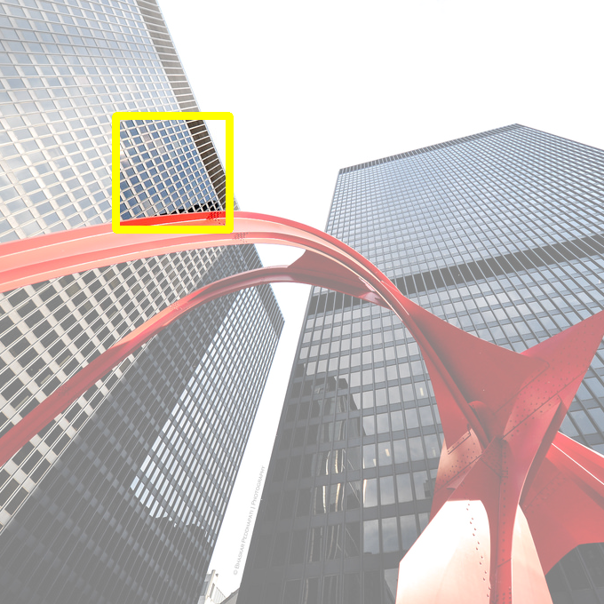
HR

SESR-M7

ABPN

EDSR

Bicubic

Ours-Small

Ours-Medium

Ours-Large

Figure 10: Visual comparison of $2\times$ super-resolution results by QuickSRNet and existing solutions on Urban100 images.

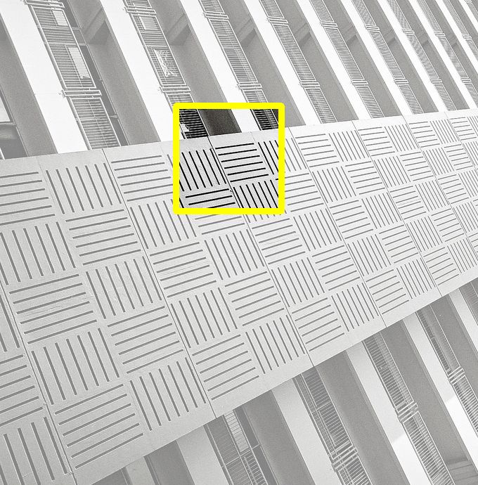
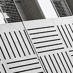
HR

SESR-M7

ABPN

EDSR

Bicubic

Ours-Small

Ours-Medium

Ours-Large

Figure 11: Visual comparison of $3\times$ super-resolution results by QuickSRNet and existing solutions on Urban100 images.

HR

SESR-M7

ABPN

EDSR

Bicubic

Ours-Small

Ours-Medium

Ours-Large

Figure 12: Visual comparison of $4\times$ super-resolution results by QuickSRNet and existing solutions on DIV2K images.

ABPN

QuickSRNet-Medium

ABPN

QuickSRNet-Medium

Figure 13: More examples of visual artifacts by ABPN vs QuickSRNet-Medium ($4\times$) on Urban 100 images.

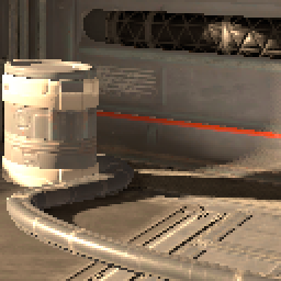
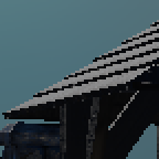
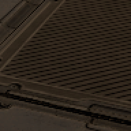
(a) LR

(b) Bicubic

(c) FSR1.0

(d) QuickSRNet-Small

Figure 14: SISR ($2\times$) for Gaming: (a) Low-resolution, (b) Bicubic interpolation, (c) FSR1.0, and (d) QuickSRNet-Small (ours).

Scaling	QuickSRNet Specification	Set5		Set14		BSD100		Urban100
Factor		FP16	INT8	FP16	INT8	FP16	INT8	FP16	INT8
2$\times$	f32 - m1	36.83	36.67	32.35	32.28	31.43	31.38	29.66	29.61
	f32 - m2 (small)	37.12	36.97	32.57	32.53	31.61	31.58	30.15	30.10
	f32 - m3	37.30	37.06	32.72	32.57	31.72	31.63	30.43	30.30
	f32 - m5 (medium)	37.39	37.22	32.82	32.75	31.82	31.77	30.75	30.66
	f32 - m7	37.51	37.27	32.95	32.84	31.88	31.81	30.93	30.84
	f32 - m11	37.59	37.19	33.00	32.86	31.95	31.80	31.14	30.91
	f64 - m11 (large)	37.87	37.61	33.29	33.18	32.12	32.04	31.74	31.64
3$\times$	f32 - m1	32.75	32.69	29.08	29.05	28.41	28.38	26.19	26.16
	f32 - m2 (small)	33.10	33.03	29.29	29.25	28.57	28.55	26.53	26.51
	f32 - m3	33.33	33.25	29.39	29.35	28.67	28.63	26.77	26.72
	f32 - m5 (medium)	33.58	33.49	29.49	29.46	28.75	28.72	27.02	26.99
	f32 - m7	33.69	33.53	29.60	29.52	28.81	28.76	27.16	27.10
	f32 - m11	33.81	33.63	29.68	29.60	28.86	28.80	27.35	27.27
	f64 - m11 (large)	34.14	34.01	29.88	29.82	29.02	28.98	27.81	27.76
4$\times$	f32 - m1	30.48	30.42	27.31	27.27	26.94	26.91	24.47	24.45
	f32 - m2 (small)	30.84	30.82	27.55	27.54	27.07	27.06	24.74	24.74
	f32 - m3	31.04	30.95	27.65	27.58	27.16	27.12	24.90	24.86
	f32 - m5 (medium)	31.27	31.21	27.79	27.76	27.24	27.21	25.08	25.06
	f32 - m7	31.39	31.29	27.83	27.80	27.30	27.27	25.22	25.18
	f32 - m11	31.50	31.36	27.93	27.85	27.35	27.29	25.32	25.27
	f64 - m11 (large)	31.77	31.73	28.15	28.12	27.50	27.48	25.74	25.72

Table 8: QuickSRNet PSNRs (dB) evaluated for different scaling factors ($2\times$, $3\times$, and $4\times$) on benchmark SISR datasets before and after quantization

Scaling	QuickSRNet Specification	Set5	Set14	BSD100	Urban100
Factor		PSNR / SSIM	PSNR / SSIM	PSNR / SSIM	PSNR / SSIM
2$\times$	f32 - m1	36.83 / 0.9563	32.35 / 0.9085	31.43 / 0.8900	29.66 / 0.8999
	f32 - m2 (small)	37.12 / 0.9575	32.57 / 0.9107	31.61 / 0.8925	30.15 / 0.9067
	f32 - m3	37.30 / 0.9583	32.72 / 0.9117	31.72 / 0.8942	30.43 / 0.9104
	f32 - m5 (medium)	37.39 / 0.9586	32.82 / 0.9130	31.82 / 0.8955	30.75 / 0.9142
	f32 - m7	37.51 / 0.9593	32.95 / 0.9136	31.88 / 0.8964	30.93 / 0.9164
	f32 - m11	37.59 / 0.9594	33.00 / 0.9142	31.95 / 0.8973	31.14 / 0.9186
	f64 - m11 (large)	37.87 / 0.9603	33.29 / 0.9166	32.12 / 0.8992	31.74 / 0.9248
3$\times$	f32 - m1	32.75 / 0.9112	29.08 / 0.8234	28.41 / 0.7880	26.19 / 0.8026
	f32 - m2 (small)	33.10 / 0.9157	29.29 / 0.8282	28.57 / 0.7919	26.53 / 0.8128
	f32 - m3	33.33 / 0.9180	29.39 / 0.8298	28.67 / 0.7947	26.77 / 0.8195
	f32 - m5 (medium)	33.58 / 0.9206	29.49 / 0.8327	28.75 / 0.7971	27.02 / 0.8266
	f32 - m7	33.69 / 0.9216	29.60 / 0.8335	28.81 / 0.7986	27.16 / 0.8303
	f32 - m11	33.81 / 0.9226	29.68 / 0.8346	28.86 / 0.8000	27.35 / 0.8347
	f64 - m11 (large)	34.14 / 0.9258	29.88 / 0.8397	29.02 / 0.8038	27.81 / 0.8459
4$\times$	f32 - m1	30.48 / 0.8659	27.31 / 0.7559	26.94 / 0.7147	24.47 / 0.7262
	f32 - m2 (small)	30.84 / 0.8741	27.55 / 0.7635	27.07 / 0.7196	24.74 / 0.7382
	f32 - m3	31.04 / 0.8773	27.65 / 0.7656	27.16 / 0.7226	24.90 / 0.7447
	f32 - m5 (medium)	31.27 / 0.8821	27.79 / 0.7699	27.24 / 0.7253	25.08 / 0.7517
	f32 - m7	31.39 / 0.8838	27.83 / 0.7709	27.30 / 0.7275	25.22 / 0.7573
	f32 - m11	31.50 / 0.8856	27.93 / 0.7729	27.35 / 0.7289	25.32 / 0.7619
	f64 - m11 (large)	31.77 / 0.8908	28.15 / 0.7797	27.50 / 0.7344	25.74 / 0.7761

Table 9: QuickSRNet PSNRs (dB) and SSIM numbers evaluated for different scaling factors ($2\times$, $3\times$, and $4\times$) on benchmark SISR datasets before quantization

Exporting QuickSRNet to ONNX for on-device profiling

Before running the model on device, we shuffle the weights of some of the convolutional layers, before depth-to-space and after space-to-depth (for $1.5\times$ model) operations. This is necessary because the data layout of PyTorch’s depth-to-space operation (CRD) is not optimized on our target device (Hexagon Processor of a mobile device with Snapdragon 8 Gen 1). For better on-device performance, the data layout needs to be changed to DCR. The appropriate method of creating a QuickSRNet model instance with the shuffled weights (in DCR format) can be done with the following steps. Below are a bunch of prerequisites to accomplish this task:

• The PyTorch implementation of QuickSRNet can be found https://github.com/quic/aimet-model-zoo/blob/torch_transformer_quicksrnet/zoo_torch/examples/superres/utils/models.py#L332-L365

• Pre-trained weights (including AIMET-quantized weights and encodings) are available https://github.com/quic/aimet-model-zoo/releases/tag/quicksrnet-checkpoint-pytorch

• A Jupyter Notebook that shows how to load and use QuickSRNet is also available https://github.com/quic/aimet-model-zoo/blob/torch_transformer_quicksrnet/zoo_torch/examples/superres/notebooks/superres_quanteval.ipynb

Step 1

Load the quantized QuickSRNet model from the checkpointed weights and encodings. With the PyTorch implementation of QuickSRNet, the model can be instantiated with the appropriately shuffled weights as follows:

⬇

import torch

\par# Use one of QuickSRNetSmall, QuickSRNetMedium or QuickSRNetLarge with the desired scaling factor.

scaling_factor = 2

model = QuickSRNetSmall(scaling_factor=scaling_factor)

\parstate_dict = torch.load(model_checkpoint_path, map_location=’cpu’)[’state_dict’]

model.load_state_dict(state_dict)

model.to(device) # ‘device‘ is one of ’cuda’ or ’cpu’

\par# Re-arrange the weights of the appropriate conv layer(s)

model.to_dcr()

\par

Step 2 (optional)

To use QuickSRNet quantized using AIMET, use the following steps:

⬇

dummy_input_shape = (1, 3, 256, 256) # Expected input shape for the model (1 x C x H x W)

dummy_input = torch.randn(dummy_input_shape)

\parsim = QuantizationSimModel(model=model,

dummy_input=dummy_input,

quant_scheme=QuantScheme.post_training_tf_enhanced,

default_output_bw=8,

default_param_bw=8)

sim.set_and_freeze_param_encodings(encoding_path=encoding_path)

sim.compute_encodings(forward_pass_callback=pass_calibration_data,

forward_pass_callback_args=(calibration_data,

scaling_factor,

use_cuda))

\par

Step 3

Export the model to ONNX:

⬇

import os

import torch

from aimet_torch.onnx_utils import OnnxExportApiArgs

\parfilename = ”<onnx_filename>”

output_dir = ”<output_dir>”

model_save_path = ”<output_dir>/<filename>.onnx”

\par# PixelUnshuffle does not map to space-to-depth without the code below

import torch.onnx.symbolic_helper as sym_help

import torch.onnx.symbolic_opset11 as opset11

from torch.onnx.symbolic_helper import parse_args, _unimplemented

\par@parse_args(’v’, ’i’)

def pixel_unshuffle(g, self, downscale_factor):

rank = sym_help._get_tensor_rank(self)

if rank is not None and rank != 4:

return _unimplemented(”pixel_unshuffle”, ”only support 4d input”)

return g.op(”SpaceToDepth”, self, blocksize_i=downscale_factor)

opset11.pixel_unshuffle = pixel_unshuffle

\par# Set ‘use_quantized‘ to ‘True‘ if exporting the quantized model, else ‘False‘

if use_quantized:

sim.export(output_dir,

filename,

dummy_input,

onnx_export_args=OnnxExportApiArgs(opset_version=11))

else:

torch.onnx.export(model, dummy_input, model_save_path, export_params=True, opset_version=11)

\par

Step 4

Convert the ONNX space-to-depth and/or depth-to-space operations to DCR:

⬇

import onnx

from onnx.helper import make_attribute

\pardef overwrite_onnx_d2s_mode_to_dcr(onnx_path):

”””Manual override of the depth-to-space mode to DCR.”””

\paronnx_model = onnx.load(onnx_path)

graph = onnx_model.graph

for node in graph.node:

if node.op_type == ’DepthToSpace’:

depth_to_space_attribute = node.attribute

\parfound = False

for idx, attr in enumerate(node.attribute):

if attr.name == ’mode’:

found = True

break

if found:

node.attribute.pop(idx)

\parnew_attr = make_attribute(’s’, ’DCR’)

new_attr.name = ’mode’

\pardepth_to_space_attribute.extend([new_attr])

onnx.save(onnx_model, onnx_path)

\paronnx_path = ”<output_dir>/<filename>.onnx” # Path to the exported ONNX file

overwrite_onnx_d2s_mode_to_dcr(onnx_path)

\par

Step 5

Re-order per-channel encodings for the quantized model to DCR:

⬇

import json

\pardef reorder_per_channel_encodings_to_dcr(encodings_path, layer_names):

”””

Used to re-arrange the per-channel encodings of the conv layer(s) preceding the final depth-to-space operation.

\parThis is necessary because the data layout of PyTorch’s depth-to-space operation (CRD) is

not optimized on device. For better on-device performance, the data layout needs to be changed

to DCR.

\parNote: in the case of per-layer quantization, this function does not do anything.

”””

\parwith open(encodings_path) as f:

encodings = json.load(f)

\parnew_encodings = encodings.copy()

to_shuffle = [key for layer_name in layer_names for key in encodings[’param_encodings’] if layer_name in key]

for key in to_shuffle:

per_channel_enc = encodings[’param_encodings’][key]

if len(per_channel_enc) > 1:

scaling_factor = int((len(per_channel_enc) / 3) ** 0.5)

new_encodings[’param_encodings’][key] = [per_channel_enc[i + k * (scaling_factor ** 2)]

for i in range(scaling_factor ** 2) for k in range(3)]

else:

# per-layer quantization: do nothing

pass

\parwith open(encodings_path, ’w’) as f:

json.dump(new_encodings, f, sort_keys=True, indent=4)

\parreorder_per_channel_encodings_to_dcr(encodings_path, [’anchor’, ’conv_last’])

\par

References

- [1] Eirikur Agustsson and Radu Timofte. Ntire 2017 challenge on single image super-resolution: Dataset and study. In Proceedings of the IEEE conference on computer vision and pattern recognition workshops, pages 126–135, 2017.
- [2] Mustafa Ayazoglu. Extremely lightweight quantization robust real-time single-image super resolution for mobile devices. In Proceedings of the IEEE/CVF Conference on Computer Vision and Pattern Recognition, pages 2472–2479, 2021.
- [3] Thomas Bachlechner, Bodhisattwa Prasad Majumder, Henry Mao, Gary Cottrell, and Julian McAuley. Rezero is all you need: Fast convergence at large depth. In Uncertainty in Artificial Intelligence, pages 1352–1361. PMLR, 2021.
- [4] Marco Bevilacqua, Aline Roumy, Christine Guillemot, and Marie Line Alberi-Morel. Low-complexity single-image super-resolution based on nonnegative neighbor embedding. 2012.
- [5] Kartikeya Bhardwaj, Milos Milosavljevic, Liam O’Neil, Dibakar Gope, Ramon Matas, Alex Chalfin, Naveen Suda, Lingchuan Meng, and Danny Loh. Collapsible linear blocks for super-efficient super resolution. Proceedings of Machine Learning and Systems, 4:529–547, 2022.
- [6] X Chen, X Wang, J Zhou, and C Dong. Activating more pixels in image super-resolution transformer. arxiv 2022. arXiv preprint arXiv:2205.04437.
- [7] Hisham Chowdhury, Rense Robert Kawiak, Gabriel Ferreira de Boer, and Lucas Xavier. Intel xess-an ai based super sampling solution for real-time rendering.(2022). In Game Developers Conference, 2022.
- [8] Hisham Chowdhury, Rense Robert Kawiak, Gabriel Ferreira de Boer, and Lucas Xavier. Intel xess-an ai based super sampling solution for real-time rendering.(2022). In Game Developers Conference, 2022.
- [9] Xiaohan Ding, Xiangyu Zhang, Ningning Ma, Jungong Han, Guiguang Ding, and Jian Sun. Repvgg: Making vgg-style convnets great again. In Proceedings of the IEEE/CVF conference on computer vision and pattern recognition, pages 13733–13742, 2021.
- [10] Chao Dong, Chen Change Loy, Kaiming He, and Xiaoou Tang. Image super-resolution using deep convolutional networks. IEEE transactions on pattern analysis and machine intelligence, 38(2):295–307, 2015.
- [11] Chao Dong, Chen Change Loy, and Xiaoou Tang. Accelerating the super-resolution convolutional neural network. In Computer Vision–ECCV 2016: 14th European Conference, Amsterdam, The Netherlands, October 11-14, 2016, Proceedings, Part II 14, pages 391–407. Springer, 2016.
- [12] Tingxing Tim Dong, Hao Yan, Mayank Parasar, and Raun Krisch. Rendersr: A lightweight super-resolution model for mobile gaming upscaling. In Proceedings of the IEEE/CVF Conference on Computer Vision and Pattern Recognition, pages 3087–3095, 2022.
- [13] Zongcai Du, Jie Liu, Jie Tang, and Gangshan Wu. Anchor-based plain net for mobile image super-resolution. In Proceedings of the IEEE/CVF Conference on Computer Vision and Pattern Recognition, pages 2494–2502, 2021.
- [14] GPUOpen-Effects. Fidelityfx-fsr2/readme.md at master · gpuopen-effects/fidelityfx-fsr2, Oct 2022.
- [15] GPUOpen-Effects. Fidelityfx-fsr2/readme.md at master · gpuopen-effects/fidelityfx-fsr2, Oct 2022.
- [16] Moritz Hardt and Tengyu Ma. Identity matters in deep learning. arXiv preprint arXiv:1611.04231, 2016.
- [17] Kaiming He, Xiangyu Zhang, Shaoqing Ren, and Jian Sun. Delving deep into rectifiers: Surpassing human-level performance on imagenet classification. In Proceedings of the IEEE international conference on computer vision, pages 1026–1034, 2015.
- [18] Lennart Heim, Andreas Biri, Zhongnan Qu, and Lothar Thiele. Measuring what really matters: Optimizing neural networks for tinyml. arXiv preprint arXiv:2104.10645, 2021.
- [19] Jia-Bin Huang, Abhishek Singh, and Narendra Ahuja. Single image super-resolution from transformed self-exemplars. In Proceedings of the IEEE conference on computer vision and pattern recognition, pages 5197–5206, 2015.
- [20] Zheng Hui, Xinbo Gao, Yunchu Yang, and Xiumei Wang. Lightweight image super-resolution with information multi-distillation network. In Proceedings of the 27th acm international conference on multimedia, pages 2024–2032, 2019.
- [21] Andrey Ignatov, Radu Timofte, Maurizio Denna, Abdel Younes, Ganzorig Gankhuyag, Jingang Huh, Myeong Kyun Kim, Kihwan Yoon, Hyeon-Cheol Moon, Seungho Lee, et al. Efficient and accurate quantized image super-resolution on mobile npus, mobile ai & aim 2022 challenge: report. In Computer Vision–ECCV 2022 Workshops: Tel Aviv, Israel, October 23–27, 2022, Proceedings, Part III, pages 92–129. Springer, 2023.
- [22] Sergey Ioffe and Christian Szegedy. Batch normalization: Accelerating deep network training by reducing internal covariate shift. In International conference on machine learning, pages 448–456. pmlr, 2015.
- [23] Diederik P Kingma and Jimmy Ba. Adam: A method for stochastic optimization. arXiv preprint arXiv:1412.6980, 2014.
- [24] Bee Lim, Sanghyun Son, Heewon Kim, Seungjun Nah, and Kyoung Mu Lee. Enhanced deep residual networks for single image super-resolution. In Proceedings of the IEEE conference on computer vision and pattern recognition workshops, pages 136–144, 2017.
- [25] Edward Liu. Dlss 2.0-image reconstruction for real-time rendering with deep learning. In GPU Technology Conference (GTC), 2020.
- [26] Edward (Shiqiu) Liu, Robert Pottorff, Guilin Liu, Karan Sapra, Jon Barker, David Tarjan, Lei Yang, Kevin Shih, Marco Salvi, Andrew Tao, and Bryan Catanzaro. Dlss 2.0 – image reconstruction for real-time rendering with deep learning. In Game Developers Conference 2020, GPU Technology Conference 2020, 2020.
- [27] Jie Liu, Jie Tang, and Gangshan Wu. Residual feature distillation network for lightweight image super-resolution. In Computer Vision–ECCV 2020 Workshops: Glasgow, UK, August 23–28, 2020, Proceedings, Part III 16, pages 41–55. Springer, 2020.
- [28] Zhi-Song Liu, Li-Wen Wang, Chu-Tak Li, and Wan-Chi Siu. Hierarchical back projection network for image super-resolution. In Proceedings of the IEEE/CVF conference on computer vision and pattern recognition workshops, pages 0–0, 2019.
- [29] David Martin, Charless Fowlkes, Doron Tal, and Jitendra Malik. A database of human segmented natural images and its application to evaluating segmentation algorithms and measuring ecological statistics. In Proceedings Eighth IEEE International Conference on Computer Vision. ICCV 2001, volume 2, pages 416–423. IEEE, 2001.
- [30] Markus Nagel, Rana Ali Amjad, Mart Van Baalen, Christos Louizos, and Tijmen Blankevoort. Up or down? adaptive rounding for post-training quantization. In International Conference on Machine Learning, pages 7197–7206. PMLR, 2020.
- [31] Markus Nagel, Mart van Baalen, Tijmen Blankevoort, and Max Welling. Data-free quantization through weight equalization and bias correction. In Proceedings of the IEEE/CVF International Conference on Computer Vision, pages 1325–1334, 2019.
- [32] Markus Nagel, Marios Fournarakis, Rana Ali Amjad, Yelysei Bondarenko, Mart Van Baalen, and Tijmen Blankevoort. A white paper on neural network quantization. arXiv preprint arXiv:2106.08295, 2021.
- [33] Adam Paszke, Sam Gross, Francisco Massa, Adam Lerer, James Bradbury, Gregory Chanan, Trevor Killeen, Zeming Lin, Natalia Gimelshein, Luca Antiga, et al. Pytorch: An imperative style, high-performance deep learning library. Advances in neural information processing systems, 32, 2019.
- [34] Chitwan Saharia, Jonathan Ho, William Chan, Tim Salimans, David J Fleet, and Mohammad Norouzi. Image super-resolution via iterative refinement. arXiv:2104.07636, 2021.
- [35] Wenzhe Shi, Jose Caballero, Ferenc Huszár, Johannes Totz, Andrew P Aitken, Rob Bishop, Daniel Rueckert, and Zehan Wang. Real-time single image and video super-resolution using an efficient sub-pixel convolutional neural network. In Proceedings of the IEEE conference on computer vision and pattern recognition, pages 1874–1883, 2016.
- [36] Sangeetha Siddegowda, Marios Fournarakis, Markus Nagel, Tijmen Blankevoort, Chirag Patel, and Abhijit Khobare. Neural network quantization with ai model efficiency toolkit (aimet). arXiv preprint arXiv:2201.08442, 2022.
- [37] Karen Simonyan and Andrew Zisserman. Very deep convolutional networks for large-scale image recognition. arXiv preprint arXiv:1409.1556, 2014.
- [38] Xintao Wang, Chao Dong, and Ying Shan. Repsr: Training efficient vgg-style super-resolution networks with structural re-parameterization and batch normalization. In Proceedings of the 30th ACM International Conference on Multimedia, pages 2556–2564, 2022.
- [39] Sergey Zagoruyko and Nikos Komodakis. Diracnets: Training very deep neural networks without skip-connections. arXiv preprint arXiv:1706.00388, 2017.
- [40] Roman Zeyde, Michael Elad, and Matan Protter. On single image scale-up using sparse-representations. In Curves and Surfaces: 7th International Conference, Avignon, France, June 24-30, 2010, Revised Selected Papers 7, pages 711–730. Springer, 2012.
- [41] Hongyi Zhang, Yann N Dauphin, and Tengyu Ma. Fixup initialization: Residual learning without normalization. arXiv preprint arXiv:1901.09321, 2019.
- [42] Jiawei Zhao, Florian Schäfer, and Anima Anandkumar. Zero initialization: Initializing neural networks with only zeros and ones. arXiv preprint arXiv:2110.12661, 2021.