Feeling Optimistic? Ambiguity Attitudes for Online Decision Making

Abstract

As autonomous agents enter complex environments, it becomes more difficult to adequately model the interactions between the two. Agents must therefore cope with greater ambiguity (e.g., unknown environments, underdefined models, and vague problem definitions). Despite the consequences of ignoring ambiguity, tools for decision making under ambiguity are understudied. The general approach has been to avoid ambiguity (exploit known information) using robust methods. This work contributes ambiguity attitude graph search (AAGS), generalizing robust methods with ambiguity attitudes—the ability to trade-off between seeking and avoiding ambiguity in the problem. AAGS solves online decision making problems with limited budget to learn about their environment. To evaluate this approach AAGS is tasked with path planning in static and dynamic environments. Results demonstrate that appropriate ambiguity attitudes are dependent on the quality of information from the environment. In relatively certain environments, AAGS can readily exploit information with robust policies. Conversely, model complexity reduces the information conveyed by individual samples; this allows the risks taken by optimistic policies to achieve better performance.

I Introduction

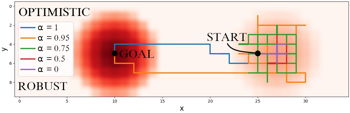
Ambiguity is a growing problem as robots are increasingly used in real-world environments. Robots face ambiguities in the form of incomplete information such as unknown terrain, conflicting sensory information, as well as vague definitions of problems and concepts. Failure to consider ambiguities in the context of decision making under uncertainty leaves robots oblivious to potential fault conditions. Despite a rich theoretical body of literature, tools for decision making under ambiguity are notably understudied [1]. Among existing solutions, robust planners are designed to recognize information gaps and ensure safe handling of worst case scenarios [2, 3]. Such a problem description aims to avoid ambiguity and will act conservatively. Robust behavior may be desirable for low uncertainty systems and safety critical systems, however, conservatism limits use of such tools in many other applications. The work here focuses on giving robots the option to trade-off between robust policies and more exploratory or optimistic policies when faced with ambiguity (Fig. 1).

Figure 1: In the tunnel world environment above, the agent is given a relatively small planning horizon, leaving the the world largely ambiguous. The agent starts near a region with small reward, but is expected to reach a region with better reward beyond its horizon. Robust policies avoid the unknown areas of the map and become stuck in the local minima. To overcome this, ambiguity attitude graph search (AAGS) employs ambiguity attitudes (specified by the tuning parameter $\alpha$) to generalize how robots consider model ambiguities. Using optimistic attitudes ($\alpha=1$), agents can actively explore and achieve a higher reward than robust attitudes ($\alpha=0$).

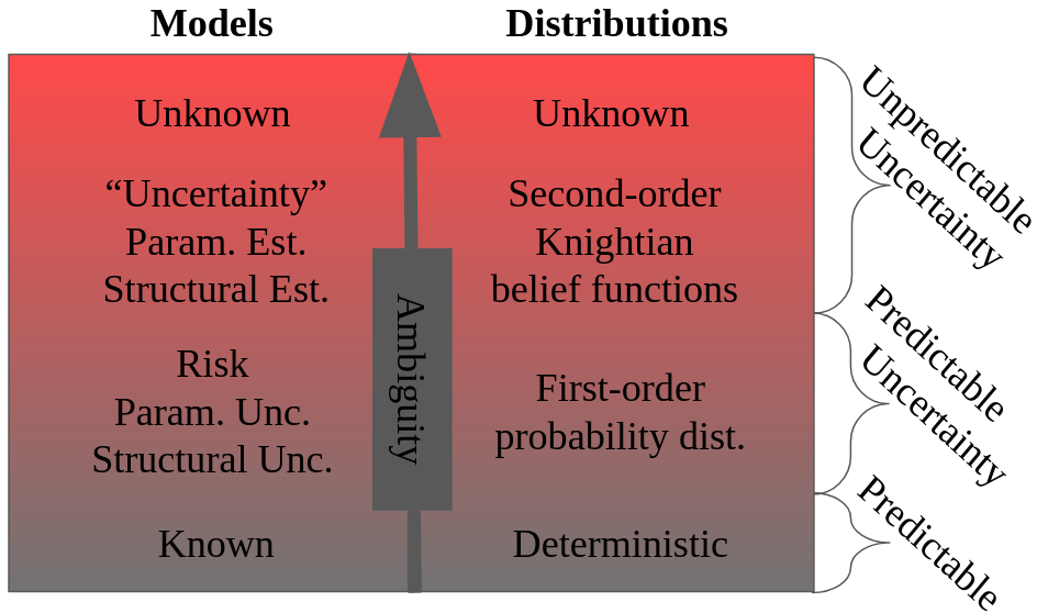
The definitions surrounding ambiguity in literature are unfortunately used loosely and are often times conflicting. We do not aim to precisely define these terms here, rather to contextualize them and better communicate the motivation of our problem. Our focus will center on two discussions: the first being the relationship between uncertainty and ambiguity in probability distributions and the second on ambiguity in the definition of models (Fig. 2).

Cuzzolin argues uncertainty is of two kinds: predictable and unpredictable [4]. Predictable uncertainty (sometimes called first-order uncertainty) is likely most familiar to us. When sampling a given probability distribution, it is expected that each outcome occurs in proportion to their likelihood function as the number of samples tends to infinity. Unpredictable uncertainties (sometimes called second-order or Knightian uncertainty [4]) are ambiguous and represent gaps in knowledge about a first-order distribution (e.g. a coin with an unknown probability of getting heads). Here the unpredictability arises when the likelihood of distinct outcomes cannot be distinguished. Such a scenario has a set of probability distributions, but we cannot define which is more “correct” due to the lack of information. It is the authors’ opinion to avoid use of the term second-order uncertainty as this is often obfuscated with parameter uncertainty. In this case, the ambiguity is implicit in the parameter estimation process [5], not the randomness of the underlying parameter distribution. In practice, this distinction may be irrelevant, but the implication is that if the parameter distribution is known, then there is no ambiguity, hence no information gap implied by the use of second-order uncertainty. Some economists brand unpredictable uncertainty and ambiguity simply as uncertainty and first-order uncertainty as risk [6, 7]. However, the robotics community tends to overload uncertainty to mean both concepts. Compare the concept of optimism in the face of uncertainty [8] with decision making under uncertainty [9]. In the prior, ambiguous distributions must be uncovered. In the latter, there is a sequential decision making problem which may have a known stochastic model. Both types of uncertainty have the concept of entropy to measure how uncertain a quantity is; in the case of unpredictable uncertainties, entropy measures ambiguity. This generalization quantifies not only how much mass is distributed to each outcome, but also to what extent mass could be distributed [4]. This is of interest in estimation processes because relatively few samples from a low entropy source are more likely to reflect the underlying distribution that a high entropy one.

Model uncertainty arises when an agent must decide from a set of possibly unknown models to describe a problem [7]. The concept of model uncertainty goes further than unpredictable uncertainties in probability distributions; it also questions the very structure and assumptions of the problem. For the purpose of this work, we restrict ourselves to the ambiguity present from estimating Markov decision process (MDP) transition probabilities with sampled data. Without loss of generality we refer to our corresponding ambiguous mass functions as models as is commonly done in literature [10, 11]. Lastly, we stress that model uncertainty is not necessarily ambiguous if the models are drawn from a known generator. While this may not appear in many problems, it is of conceptual importance as we aim to better understand the challenges in our field.

Figure 2: Ambiguity can be expressed as a continuum. An unambiguous concept is known or deterministic. In the case of randomness or stochastic processes, events may be unknown beforehand, but they occur with some known frequency. As gaps in knowledge grow, a model or distribution becomes more ambiguous or may be completely unknown. Estimation processes are attempts (often indirectly) to fill such gaps. This work focuses on estimating probability distributions representing state transition models in MDP’s. These models are represented as the belief functions described in Sec. II.

General purpose decision making tools are usually ambiguity neutral. Upper confidence trees (UCT) [12] is a good example. While its search process attempts to offset ambiguities using the number of samples, UCT arrives at its policy with the expected value of each action (an expression for which ambiguity is undefined). As mentioned above, the selection of tools which explicitly consider ambiguity are relatively limited. Among the most powerful tools for decision making under ambiguity are robust solvers such as the graph-based optimistic planning (GBOP) algorithm [8]. While robust planning offers a deeper look into the structure of ambiguity, their conservatism imposes a limit on the scope of problems they are intended to solve. This motivates the need for ambiguity attitudes, wherein an agent’s behavior can be designed to exist in the space between actively seeking out ambiguity (optimistic policies) and avoiding it (robust policies) [10, 13]. The work here extends online planning techniques to leverage ambiguous distributions and integrates ambiguity attitudes to solve a broader class of problems (Fig. 1).

This paper contributes the following:

• Ambiguity attitudes are introduced to online decision making through the novel ambiguity attitude graph search (AAGS) algorithm. This is demonstrated to generalize robust decision making and incorporates exploratory behaviors directly into an agent’s decision making process.

• A technique for evaluating sets of transition models from confidence intervals is developed. This technique maps confidence intervals to ambiguous probability mass functions known as belief functions.

Additionally, all code for environments is open source at the Interactive Robotics Laboratory gym (https://github.com/wvu-irl/irl-gym) and algorithms can be found in our decision making toolbox (https://github.com/wvu-irl/decision-making).

The remainder of the paper is as follows. Section II contains details regarding decision making under ambiguity: defining ambiguous MDP’s and belief functions. Section III describes the approach used to generate belief functions, as well as the AAGS algorithm. Section IV discusses results and identifies limitations of the proposed approach. Lastly, in Section V, the reader will find conclusions and future work.

II Ambiguity MDP

MDP’s have broad use for formulating decision problems [9, 14]. As such, they have a substantial base of literature from which to build tools. Here we extend MDP’s to ambiguous Markov decision processes (AMDP) and define belief functions from the theory of evidence. Unlike the “belief” in POMDP literature, these do not capture uncertainty in a standard mass function. Rather they generalize the concept of a mass function to support multiple outcomes [4].

While ambiguous MDP’s have been defined before [10, 11], we suggest a competing formulation. Existing frameworks are best suited to solutions with parametric distributions and problems which can be defined analytically. Conversely, the proposed AMDP formulation better supports advances from sampling based decision making tools. Define the AMDP as $\mathcal{M}\coloneqq\langle\mathcal{S},\mathcal{A},\mathcal{T},R,\gamma\rangle$. Let $s\in\mathcal{S}$ be a state in the set of states and $a\in\mathcal{A}$ be an action in the action space. The reward $R(s,a,s^{\prime})$ is a function of a given state transition. The temporal discount factor is $\gamma$. Lastly, $\mathcal{T}(s^{\prime}|s,a)$ is the set the transition models, represented here as belief functions.

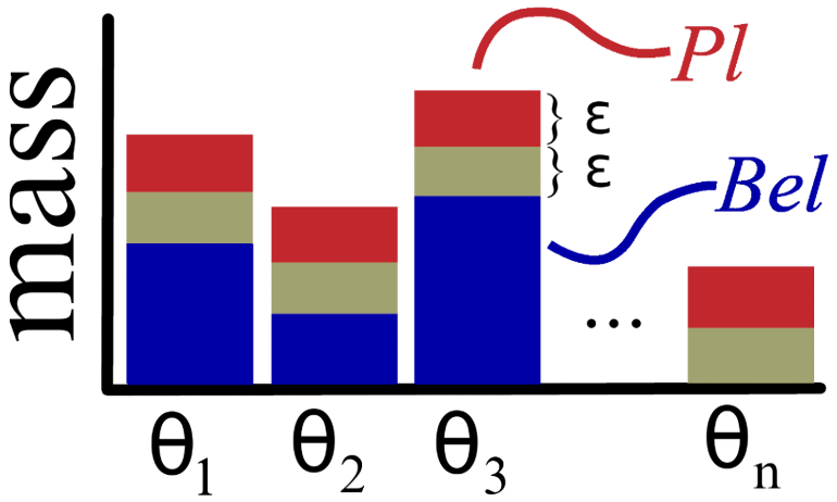
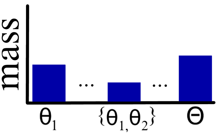
To define a model with a belief function, let $\mathcal{S}^{\prime}\subseteq\mathcal{S}$ be the space of outcomes from some state-action pair $(s,a)$. Then distribute mass to the power set of outcomes $2^{\mathcal{S}^{\prime}}$, such that the mass of some proposition $m(s^{\prime}):2^{\mathcal{S}^{\prime}}\rightarrow[0,1]$ and $\sum_{s^{\prime}}m(s^{\prime})=1$, given $s^{\prime}\in\mathcal{S}^{\prime}$ [4]. As an example let our belief function over $\mathcal{S}^{\prime}=\{s_{1},s_{2}\}$ be such that $m(\{s_{1},s_{2}\})=0.6$, $m(\{s_{1}\})=0.1$, and $m(\{s_{2}\})=0.3$. For the latter two, mass acts as is typical of a standard probability. For $m(\{s_{1},s_{2}\})$, this posits that, given our limited knowledge, 60% of the time we would be unable to predict the outcome. These belief functions are typically mapped to lower and upper probabilities rather than using the undistributed mass directly. Let there be two sets $\mathcal{B},\mathcal{C}\in\mathcal{S}^{\prime}$ The lower probability or belief represents the minimum mass supporting a set of outcomes

$$Bel(\mathcal{B})=\sum_{\mathcal{C}\subseteq\mathcal{B}}m(\mathcal{C}),$$ (1)

while the upper probability or plausibility represents corresponding maximum

$$Pl(\mathcal{B})=\sum_{\mathcal{B}\cap\mathcal{C}\neq\emptyset}m(\mathcal{C}).$$ (2)

These bounds on probability are demonstrated in Figure 3 (a) where each mass is known to $\pm\epsilon$. Figure 3 (b) captures the distribution as a belief function where mass can now support multiple hypotheses.

With a set of transition models, it is no longer possible to use Bellman’s equation and the expected value to solve the AMDP. The $\alpha$-Hurwicz function is a common choice as it allows for models with varying ambiguity attitudes [13]. More recent work sought to integrate expectation value, risk, and Knightian uncertainty into a single metric termed the additive model [6]. The added generality is unnecessary for the work here, and $\alpha$-Hurwicz has some the desirable properties explored at greater length in Sec. III-A. According to $\alpha$-Hurwicz, the value is defined as follows

$$V(s)=\max_{a}[(1-\alpha)\underline{\mathbb{E}}(s,a)+\alpha\overline{\mathbb{E}}(s,a)].$$ (3)

Here $\alpha\in[0,1]$ is a tuning parameter representing the ambiguity attitude. The lower expectation is

$$\underline{\mathbb{E}}(s,a)=min_{T\in\mathcal{T}}\sum_{s^{\prime}}T(s^{\prime}|s,a)[(r(s,a,s^{\prime})+\gamma\underline{\mathbb{E}}(s^{\prime},a^{*})].$$ (4)

The upper expectation similarly follows suit, with the $max$ function. Note that $a^{*}$ indicates the optimal action for $s^{\prime}$.

III Methods

The goal of this work is to generalize robust decision making to include ambiguity attitudes. The AAGS algorithm used to do so approximates a decision making problem as a set of models using samples from a blackbox simulator. As with several other sampling based methods [8, 9, 12, 14], agents supply an $(s,a)$-pair and the model returns observations in the form of a state transition and reward $\omega\coloneqq(s^{\prime},r)$. It is further assumed that the underlying model is an MDP with discrete state and actions spaces. AAGS is a graph-based solver, thus building up transition models for each $(s,a)$-pair. Whereas prior methods, such as GBOP, assume ambiguity is adequately described by confidence intervals, we contribute a novel way to generate belief functions from these intervals to more accurately represent the distribution of mass. Based on our mass functions upper and lower expectations are computed over the models. The online decision making algorithm AAGS then uses the specified ambiguity attitude to select the best action.

III-A Computing Belief Functions

Approximate decision making algorithms are often evaluated in part by the accuracy of estimated models. Here we concern ourselves with fixed confidence methods [15]. Such algorithms specify a confidence interval parameterized by accuracy $\epsilon$ and confidence $\delta$. The idea is that a relevant quantity $z$ is approximated with $\hat{z}$ such that $P(|z-\hat{z}|<\epsilon)\geq 1-\delta$. Whereas these bounds are generally applied to the reward or value estimates, AAGS directly bounds the mass terms instead, similar to the “knows what it knows” framework [16, 17]. In doing so, AAGS adopts a distributional perspective (shown to be more expressive than value based ones [18]). Treating the accuracy bounds as constraints, we evaluate the belief function as a linear optimization. Subsequent discounting of the model against the solution space allows us to distribute previously unused mass in the confidence term, improving the precision of our model.

(a)

(b)

Figure 3: Our approach accepts multinomial distributions estimated by collecting samples from a blackbox simulator. (a) Using confidence intervals of size $\epsilon$ for each mass term, we constrain the model. This yields upper $Pl$ and lower $Bel$ estimates on the mass of each outcome. (b) Using these bounds, we distribute the mass to a belief function. Such a formulation assigns mass to multiple hypotheses when information is ambiguous.

Begin by assuming we have a multinomial model, specified to some accuracy and confidence $(\epsilon,\delta)$. Our approach is agnostic to how these are obtained (implementation details in Appendix). We wish to redistribute the $\epsilon$ mass from each outcome to second-order mass terms, generating a set of transition models. Define $\Theta$ as the set of outcomes $(s^{\prime},r)$ from our state transition, and let $2^{\Theta}$ be the power set of all such outcomes. Let each proposition of size one be $\omega_{i}\in\Theta$ and propositions of size two or more be $\theta_{j}\in\{2^{\Theta}\setminus\Theta\}$. Given the accuracy is a confidence interval, let it constrain our belief functions such that the lower and upper bounds are, respectively, $Bel(\omega)=p_{\omega}-\epsilon$ and $Pl(\omega)=p_{\omega}+\epsilon$, $\forall\omega\in\Theta$. Let 0 and 1 bound these values, as necessary.

Using these constraints, the problem is structured as a linear optimization $Ax=B$. Note, for each proposition $\omega$,

$$Pl(\omega)-Bel(\omega)=\sum_{\omega\in\theta}m(\theta).$$ (5)

Let the columns $j$ of $A$ correspond to each $\theta_{j}$ and each row $i$ to the singleton outcomes $\omega_{i}$. Then compose the $A$ matrix using the indicator function $\mathds{1}(\omega_{i})\coloneqq\omega_{i}\in\theta_{j}$. From Eq. 5, each row of $B$ is equal to $Pl(\omega_{i})-Bel(\omega_{i})$. Next append a row of ones to the end of $A$ and $1-\sum Bel(\omega)$ to $B$ to constrain the total mass by that available. The variable $x$ is a column of all $\theta_{j}$, as these are the elements we wish to assign our mass. This optimization problem is as follows:

$$\begin{bmatrix}\lx@intercol\hfil\mathds{1}(\omega_{i})\hfil\lx@intercol\\ 1&1&...&1\end{bmatrix}\begin{bmatrix}2^{\Theta}\setminus\Theta\\ \end{bmatrix}=\begin{bmatrix}Pl(\omega_{i})-Bel(\omega_{i})\\ 1-\sum Bel(\omega_{i})\end{bmatrix}.$$ (6)

Solving for $2^{\Theta}\setminus\Theta$ yields the distribution of mass to the ambiguous terms. In practice the number of terms in $2^{\Theta}$ can become intractable. We overcome this by limiting $|\Theta|\leq 12$ and precomputing $A^{-1}$. This offered a reasonable balance between accuracy and computational constraints: storing power sets is memory intensive and online matrix inversions incur compute expenses. Outcomes were binned when the number exceeded this limit.

Next, we discount our model by the confidence to account for the chance that the true model is not within the accuracy specification. Selection of the $\alpha$-Hurwicz decision criterion has benefits here. Theory of evidence requires us to know the entire outcome space, while in our scenario, we are provided only sampled outcomes and bounds. The upper and lower expectations used in $\alpha$-Hurwicz criterion permit us to neglect these terms.

Lemma 1

Let $U\cup L\cup\Theta$ be the entire outcome space of the decision, where $U$ is the upper bound of the outcome space and $L$ the lower bound. For a given belief function $b$ over $U\cup L\cup\Theta$, inclusion of any other element $v:L\leq v\leq U$ does not change the upper $\overline{\mathbb{E}}(b)$ or lower $\underline{\mathbb{E}}(b)$ expectations.

Proof. We begin by looking at the upper expectation; the lower expectation follows trivially. By definition of the upper expectation, the mass goes to the element in each set having the greatest magnitude. All $v$ less than $U$ result in all mass allocated to $U$. If $v=U$, the terms are the same and we are left with the original set $\{U\cup L\cup\Theta\}$ of outcomes. $\square$

Let $m_{b}$ be the mass of elements in our belief function. The discounted distribution is then evaluated using the approach of [19] with the confidence as the discount parameter. Thus, the original model to $(\epsilon,\delta)$ accuracy/confidence is equivalent to the following mass function $m(\theta)=(1-\delta)m_{b}(\theta)$ for $\theta\in 2^{\Theta}$, $m(\{U\cup L\cup\Theta\})=\delta$. For simplicity, let $\theta$ now include elements of size one. This is reflected in the Algorithm 1; here $P$ is our sampled distribution. Notice in line two the accuracy is computed from the model confidence and number of samples used to make the distribution $P.N$. This is used to generate our constraints $Bel,Pl$ on the model. Notice also, that in the for loop, we are not omitting all elements in the set of outcomes $P.\Theta$, rather the proposition $\{P.\Theta\}$ itself.

$b\leftarrow\{\}$, $n=size(P)$

$Bel,Pl\leftarrow f(\delta,P.N)$

$b\leftarrow b\cup(1-\delta)Bel$

$m=A^{-1}B$

for $\theta\in\{2^{P.\Theta}\setminus\{P.\Theta\}\}$ do

       $b\leftarrow b\cup(\theta,(1-\delta)m(\theta))$

return $b\cup(\{U\cup L\cup P.\Theta\},\delta)$

Algorithm 1 dist2belief($P$,$\delta$,$U$,$L$)

III-B Ambiguity Attitude Graph Search

Our algorithm ambiguity attitude graph search (Alg. 2), generalizes robust planners to permit ambiguity attitudes. These attitudes are specified by $\alpha\in[0,1]$, where $\alpha=0$ is a conservative or a robust policy. Conversely, $\alpha=1$ is an optimistic or ambiguity seeking policy. We assume the user knows the reward bounds $R_{min}$, $R_{max}$. For an infinite horizon MDP, the bounds on the value follow as $R_{max}/(1-\gamma)$ and $R_{min}/(1-\gamma)$ [8]. Users also specify accuracy and confidence requirements $\epsilon$, $\delta$.

AAGS is a graph based planner, thus using samples more efficiently than tree methods. Assuming the simulator is much more expensive than the algorithm itself, the cost of any added computation are far outweighed by the reduced sample complexity. We allow for cyclic graphs with no constraints on connectivity. In discrete static environments, users may wish to reuse the graph, as nodes are more likely to connect to existing neighbors. Multiple independent subgraphs may occur in dynamic environments, making it preferable to throw out the graph after each iteration if reconnection is unlikely.

AAGS begins from state $s_{0}$ with an empty graph $\mathcal{G}$ and searches the solution space with $N$ trajectories up to horizon $D$. For each time step, the action having the greatest upper expectation is selected (in line with the optimism in the face of uncertainty paradigm [8]). Both the upper and lower expectations compute the belief functions from Alg. 1 internally. If a state has not been sampled enough to be considered known (i.e., satisfying the constraints $\epsilon$, $\delta$ for all actions), the generative model $G$ is sampled. Otherwise, we borrow from the “knows what it knows” framework [16] and sample the transition estimated model $T$ to reduce computational overhead. New outcomes are added to the graph and the current state is added to the list of parents. Next, our bounds are backpropagated following the approach of Leurent, et al. [8]. Therein, upper and lower bounds are updated through an approximate value iteration over the set of parents. Parents are appended to the list for those states, whose bounds have changed by more than $\beta=\dfrac{1-\gamma}{\gamma}\Delta$. Here $\Delta$ is the regret or difference in value between the second best and optimal actions for our model at a state. The key difference with respect to Leurent, et al. being we compute our upper $s.U$ and lower $s.L$ value bounds at a state through belief functions rather than confidence intervals. To conclude, the ambiguity attitude $\alpha$ and the expectations are fed into Eq. 3 to select the best action.

input: $\alpha,R_{max},R_{min},\epsilon,\delta,N,D$

initialize: $\mathcal{G}\leftarrow\{\}$

Procedure search($s_{0}$)

       if $s_{0}\not\in\mathcal{G}$ then

             $\mathcal{G}\leftarrow\mathcal{G}\cup s_{0}$,

      $n\leftarrow 0$

      while $n<N$ do

             $s\leftarrow s_{0}$

            $parents\leftarrow s$

            while $s\neq terminal$ and $depth<D$ do

                  

                  $a\leftarrow\arg\max_{b}\overline{\mathbb{E}}(s_{0},b)$

                  if $t(s,a)<t(\epsilon,\delta)$ then

                         $s^{\prime},r\sim G(s,a)$

                  else

                         $s^{\prime},r\sim T(s,a)$

                  

                  $\mathcal{G}(s,a).update(s^{\prime},r)$

                  $parents\leftarrow parents\cup s^{\prime}$, $s\leftarrow s^{\prime}$

            

            $backpropagate(parents)$

      

      $return\arg\max_{a}\alpha\underline{\mathbb{E}}(s_{0},a)+(1-\alpha)\overline{\mathbb{E}}(s_{0},a)$

Procedure backpropagate($P$)

       for $s\in parents$ do

             $parents.pop(s)$

            $L\leftarrow s.L$, $U\leftarrow s.U$

            $s.L\leftarrow\underline{\mathbb{E}}(s)$, $s.U\leftarrow\hat{\mathbb{E}}(s)$

            if $s.L-L>\beta$ or $U-s.U>\beta$ then

                   $parents\leftarrow parents\cup s.parents$

            

      

Algorithm 2 Ambiguity Attitude Graph Search

IV Results

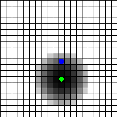
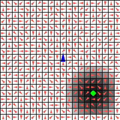
Three environments were used to evaluate AAGS. Path planning was conducted in a grid world (Fig. 4 (a)), sailing world (Fig. 4 (b)), and tunnel world (Fig. 1). These scenarios are selected to highlight interactions of ambiguity attitudes with the complexity of the environment. By analyzing grid world and sailing world, we can control the entropy of the random models to illustrate how optimistic and robust policies can both mislead agents. Tunnel world focuses on ambiguity beyond the planning horizon and illustrates how robust policies can limit an agent’s potential. Environment parameters can be found from the default parameters of the gyms at https://github.com/wvu-irl/irl-gym.

UCT [12] is used to validate the performance of AAGS. UCT was to tuned to have a rollout horizon of 25 and its exploration parameter $c$ was set to 0.5 and 8 for grid world and sailing, respectively. We draw attention to the fact that UCT is ambiguity neutral so this exploration parameter affects its search, not the final policy. In a similar way, AAGS and GBOP use optimism in the face of uncertainty to select actions during search. When it is time to select an action, however, GBOP selects a robust policy and AAGS selects one in line with its ambiguity attitude.

Because GBOP [8] is a robust planner, it is considering ambiguity to some extent. However, this does not provide a suitable foundation to compare the implications of ambiguity attitudes. To illustrate the differences of structuring ambiguity in the value estimate rather than the transition models, we extended GBOP to include ambiguity attitudes. Such an extension was trivial; vanilla GBOP provides upper and lower bounds on the value estimate so these were used with Equation 3. The new algorithm GBOP+ has vanilla GBOP as the limiting case with $\alpha=0$.

All algorithms presented here were allocated 500 samples per times step. We collected data for other values, however they were omitted due to similarity of their results. Each environment limited the number of time steps to 100. Grid world and sailing world had 325 sampled state-goal pairs for each trial considered here.

(a)

(b)

Figure 4: Example environments for (a) grid world and (b) sailing world. In grid world, the agent (blue circle) aims to reach the goal in green and is increasingly rewarded (darker regions) as it gets closer to the final goal. In sailing, the agent (blue triangle) is similarly rewarded. Though now it must try to avoid boundaries and balance following the wind (red triangles) with moving towards the goal.

IV-A For Robustness

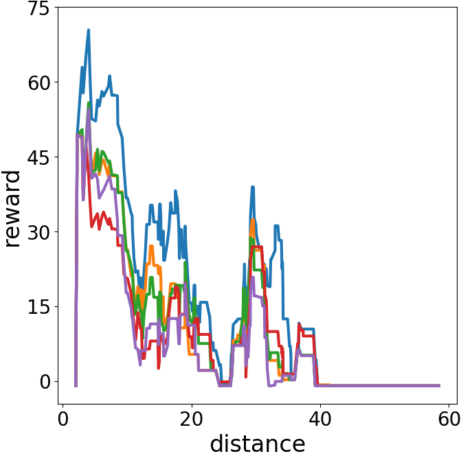
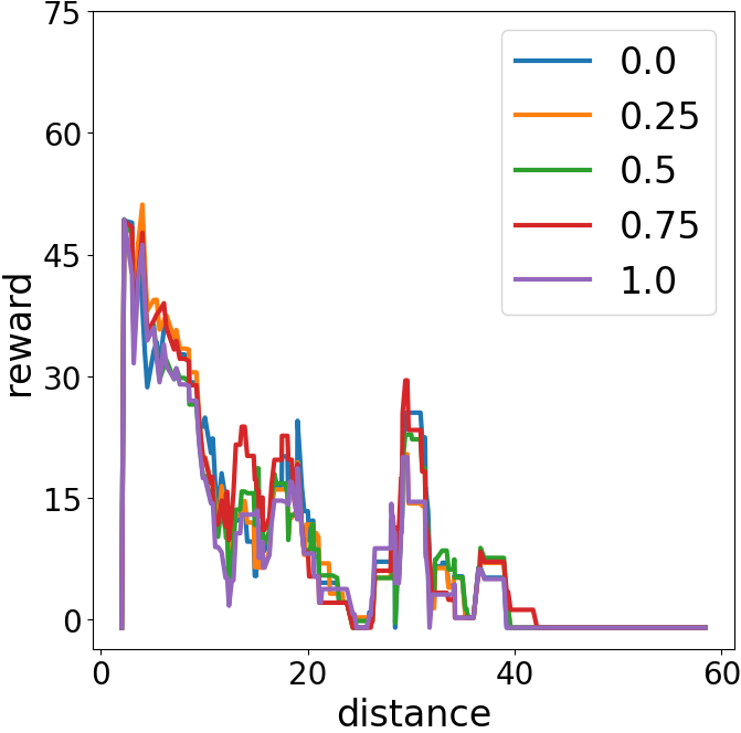
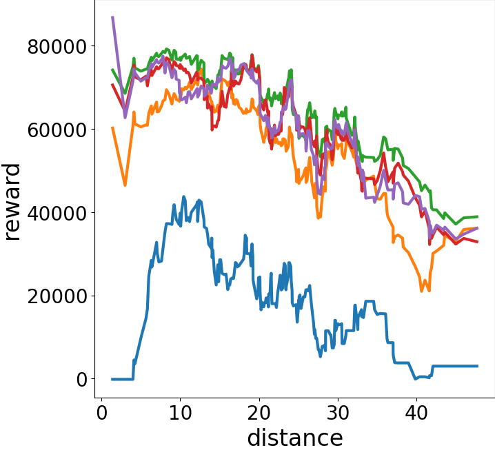
Robust policies attempt to improve the lower bound of potential outcomes [2, 3]. As a consequence, they emphasize exploiting knowledge. Exploitation can be beneficial in relatively low entropy environments, as results are likely to occur again. The grid world environment is a prime example. We take as example a 50 x 50 grid world with stochastic transitions. The robot can move to each of its four cardinal neighbors with a 10% chance of remaining in place.

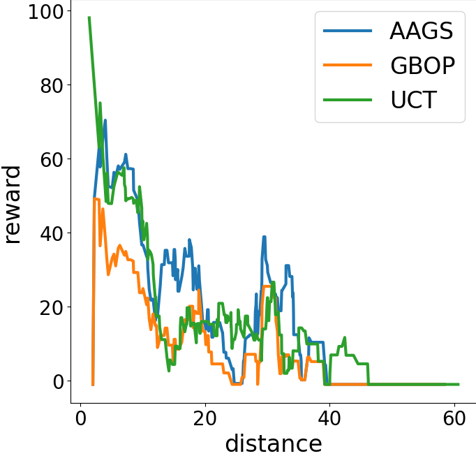
Figure 5 compares the three algorithms’ expected reward as a function of the initial distance. Conservative AAGS ($\alpha=0$) and UCT perform comparably, yielding better rewards than both GBOP+ attitudes and optimistic AAGS ($\alpha=1$). Paired with Figure 6, offers a better idea of what is happening. First, we see that the reward achieved by AAGS decreases roughly in proportion with an increase in optimism. Meanwhile, GBOP+ is largely unaffected by changes in the ambiguity attitude.

Both results are a byproduct of the relative lack of complexity in this environment. Every time the algorithms sample their environment, there is a significant possibility that result will be replicated in the actual environment. Robust policies are more inclined to follow this information, leading directly to the goal. On the other hand, optimistic policies attempt to explore the environment to ensure there is no better outcome. this leads to extra efforts despite clear signals from the environment where to go. GBOP+ has much tighter bounds than AAGS; thus it can readily detect the simplicity of the environment and converge quickly to a solution. This leaves the ambiguity attitudes with little room to change the policy.

(a)

(b)

Figure 5: Comparison of the reward achieved by each algorithm with respect to distance in grid world. In (a), AAGS and GBOP+ have conservative policies ($\alpha=0$), whereas in (b), they are optimistic ($\alpha=1$). Conservative AAGS and UCT achieve the highest rewards over the greatest distances. Both GBOP+ policies and the optimistic AAGS policy perform worse. Optimism is penalized here by unnecessary exploration because the relatively simple environment provides clear signals to the goal.

(a)

(b)

Figure 6: Comparison of the effect $\alpha$ on the reward earned by (a) AAGS and (b) GBOP+ with respect to starting distance from the goal in grid world. Due to the relative tightness of its bounds and static nature of this environment, GBOP+ converged rather quickly. Robust AAGS policies, however, were rewarded for their exploitation of the simple model behavior.

IV-B For Optimism

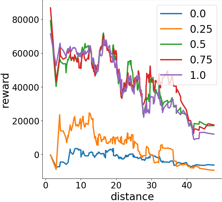
As we look to use optimistic attitudes, our study leads to more complex environments. Sailing world offers complexity on two fronts. First, inclusion of the wind directions in the state, leads to a large state space. Second, the high entropy associated with transitions in these large state spaces means the likelihood of experiencing a sampled state transition again is nearly 0. As such, the exploitation of robust policies can leave an agent chasing down fruitless outcomes. A 40 x 40 sailing world is considered, where wind is dynamic with a 10% chance of direction change. In sailing world, the agent can move forward or change direction by $\pm 45^{\circ}$; the agent is rewarded for moving towards the goal and penalized for moving against the wind or near the map borders.

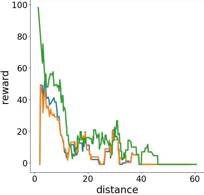
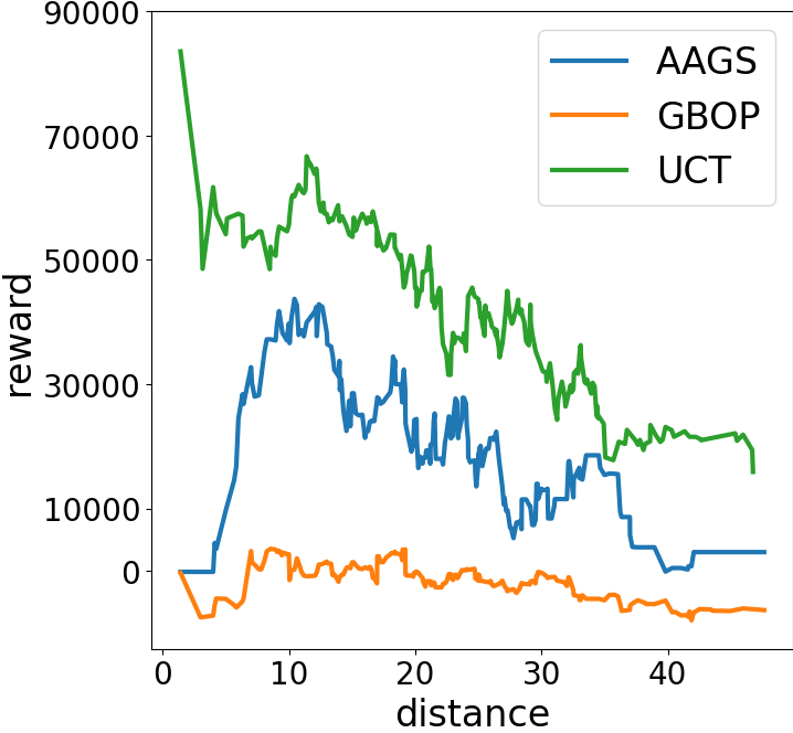
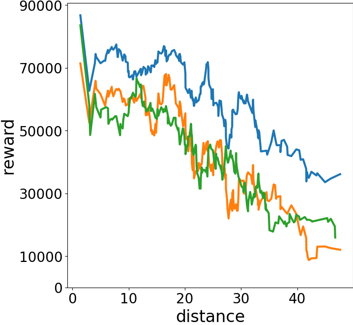
Again we begin by comparing all three algorithms (Fig. 7). In this scenario, the optimistic AAGS policies achieve the highest rewards over the greatest distances. UCT and optimistic GBOP+ policies perform well following closely behind, though they suffer greater losses as distance increases. All taper off roughly linearly with the distance. At the middle of the pack is the conservative AAGS policy. The conservative GBOP+ policy mostly avoids penalties, but does not achieve much in the way of reaching the goal. These trends are reflected in Figure 8. For both AAGS and GBOP+ conservative policies becomes mired, while even moderately optimstic policies are able to reach the goal reliably.

These results can be traced back to the increased complexity of the environment. Due to the high entropy of a large state space and dynamic transitions, states are rarely visited. Robust policies quite literally “go where the winds take them”, as the saying goes. The constant fluctuations of the wind give them conflicting signals. This leaves the agent with a noisy lower bound causing it to get lost. Conversely, optimistic policies can capture the consistent positive reward of moving toward the goal reflected in the upper bound.

(a)

(b)

Figure 7: Comparison of the reward achieved by each algorithm with respect to distance in the sailing world. In (a), AAGS and GBOP+ have conservative policies ($\alpha=0$), whereas in (b), they are optimistic ($\alpha=1$). In the optimistic scenario, AAGS has the highest and most consistent rewards. UCT and the optimistic GBOP+ follow, achieving similar results to each other. Conservative AAGS policies are met with moderate success, while conservative GBOP+ policies can do little other than avoid penalties. This demonstrates how optimistic policies can capture the consistent positive signals, but conservative policies become lost in conflicting perturbations from small penalties.

(a)

(b)

Figure 8: Comparison of the effect $\alpha$ on the reward earned by (a) AAGS and (b) GBOP+ with respect to starting distance from the goal in the sailing world. Even moderately optimistic policies are able to reach the goal consistently. Meanwhile, conservative policies are dominated by the small negative fluctuations of the wind. They are left following the wind to avoid penalties.

IV-C Optimism for Exploration

Lastly, we turn to optimism as a means of exploration. Often information will be beyond the horizon of a planner. Some works are dedicated solely to information gathering [20], but what happens when we wish to do so and perform other objectives? Optimistic ambiguity attitudes naturally induce exploratory behavior, offering a simple way to integrate exploration with other mission objectives.

For this scenario, we introduce the tunnel world (Fig. 1). In tunnel world, the agent is situated in a narrow passage near a reward that is locally substantial but globally undesirable. Some distance away there is a larger reward that is the true goal. The horizons of AAGS and GBOP+ are set to 10 steps so the world is largely unknown and the optimal goal can not be seen by the agents Given the small scale of this problem, UCT is not included as its dynamic horizon would find the goal for the number of samples given; in a future work this is a feature we would like to include with AAGS. As this is illustrative we only conduct 25 trials for each ambiguity attitude and distance (to the large reward) pair.

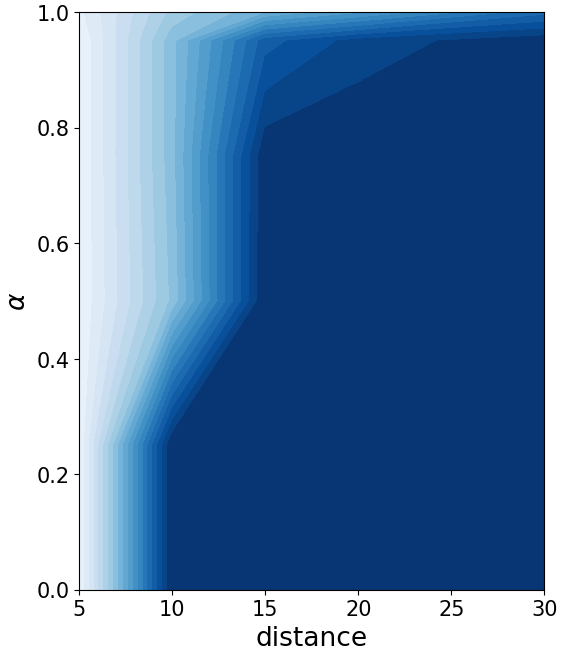
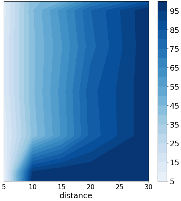
Figure 1 demonstrates AAGS attempting to reach the large goal. The search area progressively increases as ambiguity attitudes become more optimistic, until the agent can efficiently search and find the ultimate goal. Figure 9 represents this behavior as a function of the number of steps it takes to reach the final goal. With AAGS, the level of optimism need to reach the goal in a short time increases relatively quickly. GBOP+, on the other hand, has a more gradual response to the increase in distance, giving a user finer control over the exploration.

(a)

(b)

Figure 9: Controlling the distance and ambiguity attitudes of (a) AAGS and (b) GBOP+, the average number of steps required to reach the high reward goal are shown. Notice that AAGS responds rather abruptly to increases in distance. GBOP+, conversely has a more gradual response offering more control over the amount of exploration.

IV-D General Discussion

As demonstrated in the results, AAGS can solve path planning tasks with comparable performance to UCT with respect to accumulated reward and distance. More importantly, these results show the impact ambiguity attitudes can have on performance. Given that robust methods are already in use it is important to understand their limitations. Similarly, the generalization of robustness to ambiguity attitudes, motivates a need to understand optimistic behaviors as well. This is accomplished by contextualizing the result with respect to the complexity of environments and their reward structure.

IV-E Limitations

There are a few limitations the reader should be aware of. First, whereas recent approaches have sought to tie accuracy to estimates of the value and the structure of the algorithm, we have here implemented a generic mapping to estimate accuracy of a probability mass function (Appendix). Thus, the bounds on distributions in AAGS converge relatively slowly, leaving greater ambiguity in the model. AAGS, however, is designed to more precisely distribute ambiguity in the models and factors confidence into the models. While it requires more thorough study, this helps compensate for the slower convergence. This also introduces the question of whether methods can be designed to reduce ambiguity by better understanding how information gaps are distributed.

We performed analysis in discrete environments. Connectivity of graphs can be tricky in continuous domains, so this planner would behave more like a tree search without a method to abstract states. Sailing world approximates this with its large state space, however this does not appear to have negatively impacted performance. Lastly, as noted before, we artificially limit the number of outcomes to compute our bounds. This is due to storage reasons as the the $A$ matrix scales with complexity $\mathcal{O}(2^{\Theta})$. In the future, we would like to develop an error constrained method for distributing the mass.

V Conclusions

The increasing complexity of tasks we assign to robots entails increasing ambiguity. Robustness is already a consideration when developing autonomous systems. However, as demonstrated here, it is not always the best avenue when ambiguity is present. This work supports a more complete conceptualization of ambiguities in the decision making process through the introduction of ambiguity attitudes. Whereas robust attitudes avoid ambiguity and exploit their knowledge, optimistic attitudes seek ambiguity and are naturally exploratory. In simple domains with clear signals or safety critical applications, robust methods can be used to safely and efficiently reach an objective. However, as signals become more muddied (e.g., in the sailing world), taking risks can have a significant payout. Ambiguity attitudes demonstrates the flexibility to make this trade-off. The results for this work were supported by the ambiguity attitude graph search (AAGS) algorithm developed here. AAGS was shown to perform comparably to existing techniques in both general decision making under uncertainty (via UCT) and in robust decision making (via GBOP).

Looking to the future there are a few key directions this work should be taken. Among the most important are extensions to continuous domains and with partially observable MDP’s. Some work has begun in this direction [21], though they do not consider the implications of ambiguity attitudes. Furthermore, as ambiguity increases, the model assumptions come into questions, not just their probability distributions [5, 7]. Lastly, as a more exploratory measure, we consider the option of making ambiguity attitudes a function of the state. Agents could then assess for themselves the danger or payoff associated with a more or less optimistic attitude.

APPENDIX

In this paper we use confidence intervals in a few different ways. First, we wish to compute the accuracy given a confidence and the number of samples. We also use the accuracy and confidence requirements to specify a stopping rule for resampling the model. As such, it is convenient to have a relation that affords this flexibility. To arrive at one, we performed Monte Carlo trials to sample multinomial distributions and estimate the likelihood a model would meet a given accuracy. Following, we arrived at this relation

$$t(\epsilon,\delta)=\dfrac{ln\dfrac{1}{1.25(1-\delta)-1/6}}{\epsilon(-ln\dfrac{1}{1.5(1-\epsilon)+1/3})^{2}}.$$ (7)

As intuition would suggest, the following constraints are also satisfied. First, $\delta(\epsilon=1,t)=0$: no requirement on accuracy implies it is met trivially. Next, $\epsilon(\delta=0,t)=0$: no confidence in a model implies it is known to perfect precision. We found this approximation performed well and better matched the distribution than existing (algorithm agnostic) bounds [16, 17], while keeping $\epsilon,\delta\in[0,1]$. It is an open question to better approximate the relation between these values. Furthermore, algorithm specific relations may improve performance by exploiting structural components of their solution. Given the nonlinearity in $\epsilon$, we used gradient descent to find the solution.

References

- [1] A. J. Keith and D. K. Ahner, “A survey of decision making and optimization under uncertainty,” Annals of Operations Research, vol. 300, no. 2, pp. 319–353, 2021.
- [2] G. N. Iyengar, “Robust dynamic programming,” Mathematics of Operations Research, vol. 30, no. 2, pp. 257–280, 2005.
- [3] W. Wiesemann, D. Kuhn, and B. Rustem, “Robust markov decision processes,” Mathematics of Operations Research, vol. 38, no. 1, pp. 153–183, 2013.
- [4] F. Cuzzolin, The Geometry of Uncertainty: The Geometry of Imprecise Probabilities. Springer Nature, 2020.
- [5] A. H. Briggs, M. C. Weinstein, E. A. Fenwick, J. Karnon, M. J. Sculpher, and A. D. Paltiel, “Model parameter estimation and uncertainty analysis: a report of the ispor-smdm modeling good research practices task force working group–6,” Medical decision making, vol. 32, no. 5, pp. 722–732, 2012.
- [6] Y. He, J. S. Dyer, J. C. Butler, and J. Jia, “An additive model of decision making under risk and ambiguity,” Journal of Mathematical Economics, vol. 85, pp. 78–92, 2019.
- [7] M. Marinacci, “Model uncertainty,” Journal of the European Economic Association, vol. 13, no. 6, pp. 1022–1100, 2015.
- [8] E. Leurent and O.-A. Maillard, “Monte-carlo graph search: the value of merging similar states,” in Asian Conference on Machine Learning. PMLR, 2020, pp. 577–592.
- [9] M. J. Kochenderfer, Decision making under uncertainty: theory and application. MIT press, 2015.
- [10] S. Saghafian, “Ambiguous partially observable markov decision processes: Structural results and applications,” Journal of Economic Theory, vol. 178, pp. 1–35, 2018.
- [11] N. Bäuerle and U. Rieder, “Markov decision processes under ambiguity,” arXiv preprint arXiv:1907.02347, 2019.
- [12] L. Kocsis and C. Szepesvári, “Bandit based monte-carlo planning,” in European conference on machine learning. Springer, 2006, pp. 282–293.
- [13] K. J. Arrow and L. Hurwicz, “An optimality criterion for decision-making under ignorance,” Uncertainty and expectations in economics, vol. 1, 1972.
- [14] R. S. Sutton and A. G. Barto, Reinforcement learning: An introduction. MIT press, 2018.
- [15] A. Jonsson, E. Kaufmann, P. Ménard, O. Darwiche Domingues, E. Leurent, and M. Valko, “Planning in markov decision processes with gap-dependent sample complexity,” Advances in Neural Information Processing Systems, vol. 33, pp. 1253–1263, 2020.
- [16] L. Li, M. L. Littman, T. J. Walsh, and A. L. Strehl, “Knows what it knows: a framework for self-aware learning,” Machine learning, vol. 82, no. 3, pp. 399–443, 2011.
- [17] S. M. Kakade, On the sample complexity of reinforcement learning. University of London, University College London (United Kingdom), 2003.
- [18] M. G. Bellemare, W. Dabney, and R. Munos, “A distributional perspective on reinforcement learning,” in International Conference on Machine Learning. PMLR, 2017, pp. 449–458.
- [19] G. Shafer, A mathematical theory of evidence. Princeton university press, 1976, vol. 42.
- [20] J. J. Beard, Environment Search Planning Subject to High Robot Localization Uncertainty. West Virginia University, 2020.
- [21] S. Ross, B. Chaib-draa, and J. Pineau, “Bayes-adaptive pomdps,” Advances in neural information processing systems, vol. 20, 2007.