PRIMO: Private Regression in Multiple Outcomes

Abstract

We introduce a new differentially private regression setting we call Private Regression in Multiple Outcomes (PRIMO), inspired the common situation where a data analyst wants to perform a set of $l$ regressions while preserving privacy, where the covariates $X$ are shared across all $l$ regressions, and each regression $i\in[l]$ has a different vector of outcomes $y_{i}$. While naively applying private linear regression techniques $l$ times leads to a $\sqrt{l}$ multiplicative increase in error over the standard linear regression setting, in Subsection 4.1 we modify techniques based on sufficient statistics perturbation (SSP) to yield greatly improved dependence on $l$. In Subsection 4.2 we prove an equivalence to the problem of privately releasing the answers to a special class of low-sensitivity queries we call inner product queries. Via this equivalence, we adapt the geometric projection-based methods of [1] to the PRIMO setting. Under the assumption the labels $Y$ are public, the projection gives improved results over the Gaussian mechanism when $n<l\sqrt{d}$, with no asymptotic dependence on $l$ in the error. In Subsection 4.3 we study the complexity of our projection algorithm, and analyze a faster sub-sampling based variant in Subsection 4.4. Finally in Section 5 we apply our algorithms to the task of private genomic risk prediction for multiple phenotypes using data from the 1000 Genomes project. We find that for moderately large values of $l$ our techniques drastically improve the accuracy relative to both the naive baseline that uses existing private regression methods and our modified SSP algorithm that doesn’t use the projection.

1 Introduction

Linear regression is one of the most fundamental statistical tools used across the applied sciences, for both inference and prediction. In genetics, polygenic risk scores [2, 3] are computed by regressing phenotype (e.g. disease status) onto individual genomic data (SNPs) in order to identify genetic risk factors. In the social sciences, we might regress observed societal outcomes like income or marital status on a fixed set of covariates [4]. In many of these cases where the data records correspond to individuals, there are two aspects of the problem setting that co-occur:

• The individuals may have a legal or moral right to privacy that has the potential to be compromised by their participation in a study.

• Multiple regressions will be ran using the same set of individual characteristics across each regression with different outcomes, either within the same study or across many different studies.

Aspect $1$ has been established as a legitimate concern through both theoretical and applied work. The seminal paper of [5] showed that the presence of an individual in a genomic dataset could be identified given simple summary statistics about the dataset, leading to widespread concern over the sharing of the results of genomic analyses. In the machine learning setting, where what is being released is a model $w$ trained on the underlying data, there is a long line of research into “Membership Inference Attacks" [6, 7], which given access to $w$ are able to identify which points are in the training set. Over the last decade, differential privacy [8] has emerged as a rigorous solution to the privacy risk posed by Aspect $1.$ In the particular case of linear regression the problem of how to privately compute the optimal regressor has been studied in great detail, which we summarise in Subsection 3.

Aspect $2$ has been studied extensively from the orthogonal perspective of multiple hypothesis testing, but until now has not been considered in the context of privacy. The problem of overfitting or “p-hacking” in the social and natural sciences has been referred to as the “statistical crisis in science" [9], and developing methods that quantify and mitigate the effects of overfitting has been the subject of much attention in the statistics and computer science communities [10, 11, 12]. Given the ubiquity of Aspects $1$ and $2$, this raises an important question:

When computing $i=1\ldots l$ distinct regressions with a common set of $X$’s and distinct $y_{i}$’s, what is the optimal accuracy-privacy tradeoff?

Interestingly, at a technical level, the problem of multiple hypothesis testing is related to differential privacy. It has been shown that if each query (in this case regression which is a special class of query called an optimization query [13]) is computed subject to differential privacy, then we can obtain a provable tradeoff between the number of noisy query answers we provide about a dataset and the extent of overfitting that is possible [10]. This gives a second motivation beyond privacy for our setting: even when the underlying data is not sensitive, our method can be viewed as a way to provably prevent overfitting when running multiple linear regressions with shared covariates.

1.1 Results

The primary contribution of this work is to introduce the novel PRIMO problem, and to provide a class of algorithms that trade off accuracy, privacy, and computation (Subsections 4.1, 4.2). In addition to introducing the PRIMO problem, to our knowledge we are the first to apply private query release methods to linear regression (Subsection 4.2). In Subsection 4.3 we analyze the computational complexity our method, and include an analysis of sub-sampled private linear regression (Subsection 4.4). We also provide a compelling practical application of our algorithms to the problem of genomic risk prediction with multiple phenotypes using data from the 1000 Genomes project [14].

Our Algorithm 2 crucially leverages the assumption that we are in the public label setting, where $Y$ is considered public and $X$ is considered private. In genomics a person’s genome $X$ is capable of revealing an as yet untold number of sensitive insights about their health, whereas the phenotypes (outcomes) $y$ might be observable characteristics like height or eye color that are not private. We also remark that Algorithm 2 can just as easily be applied in the private label setting where $X$ is considered public and $Y$ is private, where the projection is into $C(X)$ rather than $C(Y)$ in Line $5$. This setting is known as label differential privacy, and has been the subject of increasing interest [15, 16, 17]. Since the results from the public label setting encompass the results under label DP, with the added complexity of having to add noise to the covariance matrix $X^{T}X$, we state our results for the public label setting.

We will show that in a range of common parameter settings, our methods can obtain PRIMO at minimal cost. [18] shows that for private linear regression (PRIMO with $l=1$), we have the following lower bound on the error $f(w_{private})-f(w_{opt})\geq$

$$\min\{||\mathcal{Y}||^{2},\frac{\sqrt{d}(||\mathcal{X}||^{2}||\mathcal{W}||^{2}+||\mathcal{X}||||\mathcal{W}||||\mathcal{Y}||}{n\epsilon}\}$$ (1)

Since this lower bound holds for the case when $l=1$, it of course holds for the PRIMO setting where $l>1$. Throughout the paper this lower bound will serve as a benchmark for the cost to accuracy of taking $l>1$, and in settings in which the bounds for PRIMO match this lower bound we will say we have “PRIMO for Free.”

Theorems 4.1, 4.3 imply that if $\alpha$ is the difference between mean squared error of the private estimator output by Algorithm 1 with $\mathcal{M}=\texttt{{GaussMech}}$ and $\mathcal{M}=$ Algorithm 2 respectively and the non-private OLS estimator, then with high probability:

$$\begin{split}\alpha^{2}=\tilde{O}(\frac{d||\mathcal{X}||^{4}||\hat{w}||^{4}}{n^{2}}+\min(\frac{||\hat{w}||^{2}\sqrt{d}|\mathcal{Y}|^{2}||\mathcal{X}||^{2}}{n},\frac{||\hat{w}||^{2}ld|\mathcal{Y}|^{2}||\mathcal{X}||^{2}}{n^{2}}))\end{split}$$ (2)

Guarantees of ReuseCov
$\#$ $l$ of regressions	$\alpha$	$\text{cost}(l)$	$\mathcal{M}$	Privacy
$l>\frac{n}{\sqrt{d}},n<\frac{\sqrt{d}||\mathcal{X}||^{2}||\mathcal{W}||^{2}}{|\mathcal{Y}|^{2}}$	$\tilde{O}\left(\frac{\sqrt{d}||\mathcal{X}||^{2}||\hat{w}||^{2}}{n}\right)$	1	Proj	Public $Y$
$l>\frac{n}{\sqrt{d}},n>\frac{\sqrt{d}||\mathcal{X}||^{2}||\mathcal{W}||^{2}}{|\mathcal{Y}|^{2}}$	$\tilde{O}\left(\frac{||\hat{w}||{d}^{1/4}|\mathcal{Y}|||\mathcal{X}||}{\sqrt{n}}\right)$	$\frac{n}{d^{1/4}}$	Proj	Public $Y$
$l<\min(\frac{n}{\sqrt{d}},\frac{||\mathcal{X}||^{2}||\mathcal{W}||^{2}}{|\mathcal{Y}|^{2}})$	$\tilde{O}\left(\frac{\sqrt{d}||\mathcal{X}||^{2}||\hat{w}||^{2}}{n}\right)$	1	Gauss	Private $X,Y$
$l\in(\frac{||\mathcal{X}||^{2}||\mathcal{W}||^{2}}{|\mathcal{Y}|^{2}},\frac{n}{\sqrt{d}})$	$\tilde{O}\left(\frac{||\hat{w}||\sqrt{ld}|\mathcal{Y}|||\mathcal{X}||}{n}\right)$	$\sqrt{l}$	Gauss	Private $X,Y$

Figure 1: Here $\text{cost}(l)$ is the ratio of the error for PRIMO given by Equation 2 to the lower bound in Equation 1, and $\mathcal{M}$ denotes the mechanism used to compute $X^{T}Y$.

In Figure 1 we summarize the accuracy guarantees implied by Equation 2. When $\text{cost}(l)=1$ this corresponds to “PRIMO for Free", and when $\text{cost}(l)=\sqrt{l}$ our upper bound matches that of the naive private baseline (Equation 6).

In Section 4.1 we adapt the previously proposed sufficient statistics perturbation (SSP) algorithm of [19, 20] to the PRIMO setting. Methods based on SSP rely on perturbing $X^{T}{X}\approx\Sigma$ and $X^{T}y\approx\Sigma_{Xy}$ separately, and then use these noisy estimates to compute the least squares estimator:

$$\tilde{w}_{i*}=\underbrace{(X^{T}X+E_{1})^{-1}}_{\text{noisy covariance term }\tilde{\Sigma}}\;\;\;\times\underbrace{(X^{T}Y_{i}+E_{2i})}_{\text{noisy association term }\tilde{\Sigma}_{Xy}}$$ (3)

Via a novel accuracy analysis of SSP for the case when the privacy levels for $E_{1},E_{2i}$ differ (Theorem 4.1), we show that since the noisy covariance matrix is reused across the regressions (as it only depends on $X$), by allocating the majority of our privacy budget to computing this term, we are able to obtain PRIMO for Free when $l<\min(\frac{n}{\sqrt{d}},\frac{||\mathcal{X}||^{2}||\mathcal{W}||^{2}}{|\mathcal{Y}|^{2}})$. When $l$ is sufficiently small, we obtain PRIMO for Free because the error term is dominated by the error in computing the noisy covariance matrix, which does not depend on $l$, rather than the error from computing the noisy association term.

Given that our PRIMO for Free result in Subsection 4.1 relies on taking $l$ small enough that the error is dominated by the covariance error term, it is natural to ask if, under parameter regimes where the error from the association term dominates, if we can obtain improved dependence of $\alpha$ on $l$ over the $\sqrt{l}$ given by the Gaussian Mechanism. This is the focus of Subsection 4.2, where we start by showing that when we assume the labels $Y$ are public, privately computing $\frac{1}{n}X^{T}Y$ is equivalent to releasing $dl$ “low sensitivity” queries [11] we call inner product queries (Definition 2.3). Our Algorithm 2 for privately answering these queries with low $l_{2}^{2}$ error is similar to the relaxed projection mechanism of [21], with a few key differences we elaborate on in Section 3. Via a refined analysis of this mechanism that exploits the geometric structure of our queries we obtain the surprising result that it is possible to completely remove the dependence of the error in computing the noisy association term on $l$ and improve the dependence on $d$ by a factor of $d^{1/4}$ – albeit at the cost of a factor of $\sqrt{n}$ (Theorem 4.2).

Theorem 4.3 states the error for PRIMO of the variant of Algorithm 1 that uses this projection mechanism as a subroutine. Inspecting the accuracy bound, we see that when $l>\frac{n}{\sqrt{d}}$ but $\frac{n}{\sqrt{d}}<\frac{||\mathcal{X}||^{2}||\mathcal{W}||^{2}}{|\mathcal{Y}|^{2}}$ we also obtain PRIMO for Free. This is in contrast to when we obtained PRIMO for Free for small $l$ in Subsection 4.1. In this case it is because (i) $l$ is sufficiently large such that the error of the noisy association term when computed via Algorithm 2 is lower than when using the Gaussian Mechanism (Lemma 1) and (ii) $n$ is sufficiently small such that the noisy covariance term dominates the error of the projection mechanism.

In Subsections 4.3, 4.4 we consider the computational complexity of our methods. In Subsection 4.3 we show that given the QR decomposition of the noisy covariance matrix and the SVD of the label matrix $Y$, standard techniques give a simple way to compute the private estimators for all $l$. When $n>d>l$ the cost of SSP variants like our ReuseCov algorithm, are dominated by the cost of forming the covariance matrix, which is $O(nd^{2})$ – prohibitively large for large $n,d$. To address this shortcoming, in Section 4.4 we develop a sub-sampling based version of ReuseCov which estimates the covariance matrix using a random sample of $s$ points – reducing the computational cost to $O(sd^{2})$.

2 Preliminaries

We start by defining the standard linear regression problem. Given $X\in\mathcal{X}^{n}\subset\mathbb{R}^{n\times d},y_{i}\in\mathcal{Y}^{n}$, and parameter space $\mathcal{W}$, for $w\in\mathcal{W}$ let $f(w)\vcentcolon=\frac{1}{n}\sum_{k=1}^{n}(w\cdot x_{k}-y_{ik})^{2}$ be the linear regression objective, and denote by $w_{i*}=\operatorname*{arg\,min}_{w}f(w)=(X^{T}X)^{-1}X^{T}y_{i}$ the ordinary least squares estimator (OLS). Let $f_{\lambda}(w)=\frac{1}{n}\sum_{k=1}^{n}(w\cdot x_{k}-y_{ik})^{2}+\lambda||w||_{2}^{2}$ the ridge regression objective, and let $w_{i*}^{\lambda}=\operatorname*{arg\,min}_{w}f_{\lambda}(w)=(\frac{1}{n}X^{T}X+\lambda I_{d})^{-1}\frac{1}{n}X^{T}y_{i}$.

The definition of data privacy we use throughout is the popular $(\varepsilon,\delta)$-differential privacy introduced in [22]. We refer the reader the to [8] for an overview of the basic properties of $(\varepsilon,\delta)-DP$ including closure under post-processing and advanced composition.

Definition 2.1.

Let $\mathcal{M}:(\mathcal{X}\times\mathcal{Y})^{n}\to\mathcal{O}$ a randomized algorithm taking as input a dataset of $n$ records. We say that $(X,Y)\sim(X^{\prime},Y^{\prime})\in(\mathcal{X}\times\mathcal{Y})^{n}$ if $\exists x,yx^{\prime},y^{\prime}$ such that $(X,Y)\cup\{x^{\prime},y^{\prime}\}/\{x,y\}=(X^{\prime},Y^{\prime})$. Then we say that $\mathcal{M}$ is $(\varepsilon,\delta)$-DP if $\forall(X,Y)\sim(X^{\prime},Y^{\prime}),o\subset\mathcal{O}$:

$$\Pr[\mathcal{M}(X,Y)\in o]\leq e^{\varepsilon}\Pr[\mathcal{M}(X^{\prime},Y^{\prime})\in o]+\delta$$ (4)

In the less restrictive case where Equation 4 holds only over adjacent $X\sim X^{\prime}$ with the same fixed $Y$, we say that we have differential privacy in the public label setting, which we consider in Section 4.2.

We now formalize the Private Regression In Multiple Outcomes (PRIMO) problem.

Definition 2.2.

PRIMO. Let $x_{i}\in\mathcal{X}\subset\mathbb{R}^{d},y_{ij}\in\mathcal{Y},$ for $i=1\ldots n,j=1\ldots l$. Let $X_{n\times d}$ the matrix with $i^{th}$ row $x_{i}$, and let $Y_{n\times l}$ the matrix with $j^{th}$ column $y_{j}=(y_{1j},\ldots y_{nj})$. The optimal solution $W^{*}$ to the PRIMO problem is

$$W^{*}=\inf_{W\in\mathcal{W}^{l}\subset\mathbb{R}^{d\times l}}||XW-Y||_{F}^{2}$$

Given a randomized algorithm $\mathcal{M}:(\mathcal{X}\times\mathcal{Y}^{l})^{n}\to\mathcal{W}^{l}$, we say that $\mathcal{M}$ is an $(\alpha,\beta,\varepsilon,\delta)$ solution to the PRIMO problem if (i) $\mathcal{M}$ is $(\varepsilon,\delta)$-DP with respect to $(X,Y)$ (or just $X$ in the public label setting), and (ii) with probability $1-\beta$ over $\tilde{W}\sim\mathcal{M}$:

$$l^{2}_{W}(X,Y)=\frac{1}{nl}||X\tilde{W}-Y||_{F}^{2}-\frac{1}{nl}||XW^{*}-Y||_{F}^{2}<\alpha$$

We will use $y_{j}$ to denote the vector of $n$ outcomes for the $j^{th}$ outcome, and $y^{i}$ for the vector of $l$ outcomes corresponding to individual $i\in[n]$.

The $(\epsilon,\delta)-DP$ algorithm we will use most throughout is the Gaussian Mechanism. Note that we state a version of the Gaussian mechanism with constant $c(\epsilon,\delta)$ that is valid for all $\epsilon>0$ (including $\epsilon>1$), which follows from analyzing the mechanism using Renyi DP [23] and converting back to $(\epsilon,\delta)$-DP.

Lemma 1.

GaussMech$(\varepsilon,\delta,\Delta)$ [8] Let $f:\mathcal{X}^{n}\to\mathbb{R}^{d}$ an arbitrary $d$-dimensional function, and define it’s sensitivity $\Delta_{2}(f)=\sup_{X\sim X^{\prime}}||f(X)-f(X^{\prime})||_{2}$, where $X\sim X^{\prime}$ are datasets that differ in exactly one element. Then the Gaussian mechanism releases $f(X)+\mathcal{N}(0,\sigma^{2}$), and is $(\varepsilon,\delta)$-differentially private for $\sigma\geq c(\varepsilon,\delta)\Delta_{2}(f)$, where $c(\varepsilon,\delta)=\sqrt{2(\frac{1}{\epsilon}+\frac{\log\frac{1}{\delta}}{\varepsilon^{2}}})$.

Lastly, we define a new class of “low-sensitivity” queries [11] we call “inner product" queries that we will make heavy use of in Subsection 4.2.

Definition 2.3.

Inner Product Query. Let $\mathcal{X}\subset\mathbb{R}^{d}$ and $X\in\mathcal{X}^{n}\subset\mathbb{R}^{d\times n}$ a dataset with column $j$ corresponding to $x_{j}\in\mathcal{X}$. Let $y\in\mathbb{R}^{n}$, and $i\in[d]$. Then the pair $(i,y)$ defines an inner product query $q_{(i,y)}:\mathcal{X}^{n}\to\mathbb{R}$,

$$q_{(i,y)}(X)\vcentcolon=\frac{1}{n}\sum_{j=1}^{n}X_{ij}y_{j}=\frac{1}{n}e_{i}^{T}Xy,$$

where $e_{i}$ is the $i^{th}$ basis vector in $\mathbb{R}^{d}$.

The $l_{2}$ sensitivity $\Delta_{2}(q_{(i,y)})$ is $\frac{||\mathcal{X}||_{\infty}|\mathcal{Y}|}{n}$, since changing one row of $i$ of $X$ changes at most one entry $\frac{1}{n}x_{ki}y_{ji}$ of $x_{k}^{t}y_{j}\leq\frac{||\mathcal{X}||_{\infty}|\mathcal{Y}|}{n}$.

Throughout the paper given a vector $v$ and matrix $A$, $||v||,||A||$ denote the $l_{2}$ and the spectral norm respectively, $||A||_{F}$ is the Frobenius norm, $||\mathcal{X}||=\sup_{x\in\mathcal{X}}||x||_{2}$, and $||\mathcal{W}||=\sup_{w\in\mathcal{W}}||w||_{2}$.

3 Related Work

Private Linear Regression.

Private linear regression is well-studied under a variety of different assumptions on the data generating distributions and parameter regimes. Typically analysis of private linear regression is done either under the fully agnostic setting where only parameter bounds $||\mathcal{X}||,|\mathcal{Y}|,||\mathcal{W}||$ are assumed, under the assumption of a fixed design matrix and $y$ generated by a linear Gaussian model (the so-called realizable case), or under the assumption of a random design matrix [24]. In this paper we focus on the first fully agnostic setting, because in our intended applications within the social and biomedical sciences in general we neither have realizability or Gaussian covariates. In the fully agnostic setting [25] provides a comprehensive survey of existing private regression approaches and bounds, including proposing a new adaptive technique.

Broadly speaking, techniques for private linear regression fall into $4$ classes, sufficient statistics perturbation (SSP) [19, 20], Objective Perturbation (ObjPert) [26], Posterior sampling [27], and privatized (stochastic) gradient descent (NoisySGD) [28]. The methods in this paper are a sub-class of SSP-based methods, which correspond to Algorithm 1 where $l=1$.

In the fully agnostic case, there are two regimes for private linear regression, each with upper bounds on empirical risk achieved by the algorithms above, and corresponding lower bounds stated below. The regimes depend on how well-conditioned the covariance matrix $X^{T}X$ is. Letting $\alpha^{*}$ be the inverse condition number we have the following lower bounds from [18]:

• When $\alpha^{*}\geq\frac{d^{1}.5(||\mathcal{X}||||\mathcal{W}||_{|}\mathcal{Y}|}{n||\mathcal{X}||||\mathcal{W}||\varepsilon}$, then:

  $$f(\hat{w})-f(w^{*})\geq\min\{|\mathcal{Y}|^{2},\frac{d^{2}(||\mathcal{X}||||\mathcal{W}||+|\mathcal{Y}|)^{2}}{n^{2}\alpha^{*}\varepsilon^{2}}\}$$

• We always have (even when $X^{T}X$ is ill-conditioned), $f(\hat{w})-f(w^{*})\geq$

  $$\min\{|\mathcal{Y}|^{2},\frac{\sqrt{d}(||\mathcal{X}||^{2}||\mathcal{W}||^{2}+||\mathcal{X}||||\mathcal{W}|||\mathcal{Y}|}{n\varepsilon}\}$$ (5)

Two techniques, NoisySGD and ObjPert both achieve the minimax lower bounds in both settings, although in order to achieve the minimax rates their hyperparameters depend on the unknown $||\mathcal{W}||$ and $\alpha^{*}$, and so [25] proposes two adaptive methods that are based on Sufficient Statistics Perturbation, and are able to achieve optimal bounds in both settings. In Subsections 4.1,4.4 we state our theoretical results under the ill-conditioned setting as it is the most general, although analogous results hold in the well-conditioned setting as well.

Now given any $(\varepsilon,\delta)$-DP algorithm for computing $w_{j}$ privately, we can use it as a sub-routine to solve PRIMO by simply running it $l$ times to compute each row of $W$. Hence by running any of the optimal algorithms $l$ times with parameters $\varepsilon^{\prime}\approx\varepsilon/\sqrt{l},\delta^{\prime}\approx\delta/l$, by advanced composition for differential privacy [8] we can achieve, subject to $(\varepsilon,\delta)$-DP:

$$\alpha=\tilde{O}(\frac{\sqrt{ld}(||\mathcal{X}||^{2}||\mathcal{W}||^{2}+||\mathcal{X}||||\mathcal{W}|||\mathcal{Y}|}{n\varepsilon})$$ (6)

So for a fixed privacy budget $\varepsilon$, this naive baseline is a factor of $\sqrt{l}$ worse than in the standard private regression setting where $l=1$.

Query Release.

In Subsection 4.2 we show that privately computing the association term $\frac{1}{n}X^{T}Y$ is equivalent to the problem of differentially privately releasing a set of $l\cdot d$ low-sensitivity queries [11]. While less is known about the optimal $l_{2}$ error for arbitrary low-sensitivity queries, it is clear that geometric techniques based on factorization and projection do not (at least obviously) apply, since there is no corresponding notion of the query matrix $A_{\mathcal{Q}}$ [29]. In the case where $X,Y$ are both private, this corresponds to releasing a subset of $l\cdot d$ $2$-way marginal queries over $d+l$ dimensions, which is well-studied [30, 31, 32]. In the related work section of the Appendix we discuss why applying existing algorithms for private release of marginals seems unlikely be able to both improve over the Gaussian Mechanism and achieve non-trivial error. However, in the less restrictive but still practically relevant setting where the labels $Y$ are public, computing the association term $\frac{1}{n}X^{T}Y$ is equivalent to the problem of differentially privately releasing a special class of $dl$ “low-sensitivity" queries we term “inner product queries" (Definition 2.3). For this special class of queries we can adapt the projected Gaussian Mechanism of [21] that is optimal for linear queries under $l_{2}$ error in the sparse regime. We are able to obtain greatly improved results over the naive Gaussian Mechanism in the regime where $l>\frac{n}{\sqrt{d}}$, as summarised in Figure 1 and presented in Subsection 4.2. This is a key regime of interest, particularly for genomic data, where $d$ the number of SNPs could be in the hundreds of millions, $n$ the population size in the hundreds of thousands ($\sim 400K$ for UK Biobank [33] one of the most popular databases), and $l$ the number of recorded phenotypes could be in the thousands.

Projection mechanisms and Algorithm 2.

Since we make heavy use of projection mechanisms in Subsection 4.2 in the public label setting, we elaborate on the difference between the existing methods and our Algorithm 2. The most technically related work to our Algorithm 2 is [21], which is itself a variant of the projection mechanism of [1]. There are several key differences in our analysis and application.The projection in [1] is designed for linear queries over a discrete domain, and runs in time polynomial in the domain size. Algorithm 2 allows continuous $\mathcal{X},\mathcal{Y}$ and runs in time polynomial in $n,d,l$. Like the relaxed projection mechanism [21], when our data is discrete we relax our data domain to be continuous in order to compute the projection more efficiently. Unlike in their setting which attempts to handle general linear queries, due to the linear structure of inner product queries our projection can be computed in polynomial time via linear regression over the $l_{2}$ ball, as opposed to solving a possibly non-convex optimization problem. Moreover, due to this special structure we can use the same geometric techniques as in [1] to obtain theoretical accuracy guarantees (Theorem 4.2).

[1] bound the accuracy of their mechanism with respect to the expected mean squared error. Due to the necessity of analyzing the error of private regression with a high probability bound, rather than expected error, we prove a high probability error bound for the accuracy of the projection mechanism (Theorem 4.2). This requires application of the Hanson-Wright Inequality for anisotropic sub-Gaussian variables [34].

Further background on private query release for linear and low-sensitivity queries under $l_{\infty}$ and $l_{2}$ error is included in the Appendix. We also include further background on sub-sampled linear regression (Subsection 4.4) in the Appendix.

4 Methods

In Subsection 4.1 we develop our SSP-variant ReuseCov as a solution to the PRIMO problem. We give an error analysis of SSP for private linear regression where the noise levels for the covariance and association terms differ, and use this to examine when the asymptotic error of PRIMO matches the error of private linear regression ("PRIMO for Free"). In Subsection 4.2 we focus on the noisy association term, and give a reduction to the problem of private release of low-sensitivity queries. We show that for sufficiently large $l$, computing the association term via projection Algorithm 2 gives a polynomial improvement in error over the Gaussian mechanism when $l$ is sufficiently large. In Subsection 4.3 we address the computational complexity of Algorithm 3. Finally, in Subsection 4.4 we address the high computational cost of computing the full covariance matrix $X^{T}X$ in $O(nd^{2})$, and show how sub-sampling the covariance matrix allows us to trade-off computation with accuracy.

4.1 ReuseCov

$\lambda-\texttt{{ReuseCov}}$

Algorithm 1 Input: $s,\lambda,\mathcal{X}\in\mathcal{X}^{n}\subset\mathbb{R}^{d\times n}$, $Y=[y_{1},\ldots y_{l}]\in\mathcal{Y}^{l\times n},$ privacy params: $\epsilon,\delta$

1:  Draw $E_{1}\sim N_{d(d+1)/2}(0,\sigma_{1}^{2}),$ where $\sigma_{1}=\frac{1}{s}c(\epsilon,\delta)||\mathcal{X}||^{2}/\epsilon$

2:  Compute $\hat{I}=(\frac{1}{n}X^{T}X+E_{1}+\lambda I)^{-1}$

3:  Draw $\hat{v}=[\hat{v}_{1},\ldots\hat{v}_{l}]\sim\mathcal{M}(\epsilon/2,\delta/2,X,Y)$

4:  for $i=1\ldots l$ 

5:     Set $\hat{w_{i}}=\hat{I}\hat{v}_{i}$

6:  end for

7:  Return $\hat{W}=[\hat{w_{1}},\ldots\hat{w_{l}}]$

In the analysis of the ridge regression variant of SSP, which corresponds to Algorithm 1 with $l=1$, Equation $13$ in [25] shows w.p. $1-\rho:$

$$\begin{split}f(\tilde{w}_{\lambda})-f(w_{i*})=\tilde{O}\left(\underbrace{\frac{d}{(\lambda+\lambda_{\min})\epsilon^{2}}||\mathcal{X}||^{2}|\mathcal{Y}|^{2}}_{\text{association error term}}+\underbrace{\frac{d}{(\lambda+\lambda_{\min})\epsilon^{2}}||\mathcal{X}||^{4}||\mathcal{W}||^{2}}_{\text{covariance error term}}\right)+\underbrace{\lambda||\mathcal{W}||^{2}}_{\text{error due to ridge penalty}}\end{split}$$ (7)

Inspecting these terms, we see that when $||\mathcal{X}||||\mathcal{W}||\gg||\mathcal{Y}||$ the error is dominated by the cost of privately computing $X^{T}X$, rather than privately computing $X^{T}y$. We now turn back to our PRIMO setting, and imagine independently applying SSP to solve each of our $l$ regression problems. By the lower bounds in [18], given a fixed privacy budget this incurs at least a $\sqrt{l}$ multiplicative blow up in error. However, we notice that when our private linear regression subroutine is an SSP variant, this naive scheme, of running $l$ independent copies of SSP is grossly wasteful. Since the $X$ matrix is shared across the different regression, we can simply compute our noisy estimate of $X^{T}X$ once, and then share that noisy covariance matrix across all of our regressions. Combining these two observations, we present Algorithm 1, where $\mathcal{M}$ can be any $(\epsilon/2,\delta/2)$-DP algorithm for estimating $X^{T}Y$.

In line $2$ we take $\epsilon_{1}=\epsilon/2$, and $\epsilon_{2}=\tilde{O}(\frac{\epsilon}{\sqrt{l}})$, allocating most of our privacy budget for the “harder" one-shot task of computing $X^{T}X$, and thus necessarily adding more noise to the association term. By advanced composition [8] this ensures $(\epsilon,\delta)$ privacy overall, and propagating these noise terms into Equation 7 gives:

Theorem 4.1.

With $\mathcal{M}=\texttt{{GaussMech}}(\epsilon/2,\delta/2,\Delta=\frac{1}{n}\sqrt{l}||\mathcal{X}|||\mathcal{Y}|)$, Algorithm 1 is an $(\alpha,\rho,\epsilon,\delta)$ solution to the PRIMO problem with

$$\alpha=\tilde{O}\left(||\hat{w}||\sqrt{\frac{d||\mathcal{X}||^{4}||\hat{w}||^{2}}{n^{2}}+\frac{ld|\mathcal{Y}|^{2}||\mathcal{X}||^{2}}{n^{2}}}\right),$$ (8)

where $||\hat{w}||^{2}=\frac{1}{l}||W^{*}||_{F}^{2}$, and $\tilde{O}$ omits terms polynomial in $\frac{1}{\epsilon},\log(1/\delta),\log(1/\rho)$.

While we defer the formal proof to the Appendix, the proof follows the analysis in [25] that uses Lemma 8 (essentially the Woodbury matrix inversion formula) to expand the difference $||\tilde{w}_{i*}-w_{i*}||_{X^{T}X}$ into the form in Equation 23 in the Appendix:

$$\begin{split}O\left(\underbrace{||E_{1}w_{i*}||_{(X^{T}X+\lambda I)^{-1}}^{2}}_{\text{covariance error}}+\underbrace{\lambda^{2}||w_{i*}||_{(X^{T}X+\lambda I)^{-1}}^{2}}_{\text{regularization error}}\right)+\tilde{O}\left(\underbrace{||E_{2}||^{2}_{(X^{T}X+\lambda I)^{-1}}}_{\text{association error}}\right)\end{split}$$ (9)

The bound follows from using a Johnson-Lindenstrauss type lemma (Lemma 11) to bound the $||E_{1}||,||E_{2}||$ terms, substituting in the noise levels in Algorithm 1, and optimizing over $\lambda$.

Inspecting Theorem 4.1, we see that when $l<\min(\frac{n}{\sqrt{d}},\frac{||\mathcal{X}||^{2}||\mathcal{W}||^{2}}{|\mathcal{Y}|^{2}})$, Algorithm 1 with $\mathcal{M}$ the Gaussian mechanism achieves error $\tilde{O}\left(\frac{\sqrt{d}||\mathcal{X}||^{2}||\hat{w}||^{2}}{n}\right)$. Since this matches the lower bound in Equation 1 for a single private regression in this case we say that we have achieved "PRIMO for Free."

4.2 Private Query Release

The improvement of Algorithm 1 over the naive PRIMO baseline in the previous sections make heavy use of the fact that the asymptotic error is dominated by the covariance error term. In the case when $\mathcal{M}$ is the Gaussian mechanism, if we are in the regime where the association term dominates, ReuseCov still incurs a $\sqrt{l}$ multiplicative factor in the error term, which does not improve over the baseline. In this section we show that via a reduction from computing the association term to private query release of inner product queries, under the weaker public label setting we can obtain improved bounds for PRIMO over the naive baseline and ReuseCov with $\mathcal{M}=\texttt{{GaussMech}}$ when $l>\frac{n}{\sqrt{d}}$.

Let us reconsider the problem of privately computing the association term $\frac{1}{n}X^{T}Y$ where $Y\in\mathcal{Y}^{n\times l}$, and $X\in\mathcal{X}^{n}\subset\mathbb{R}^{d\times n}$, and $Y$ is considered public, so our data release needs only be DP in $X$. Consider entry $(k,j)$ of $\frac{1}{n}X^{T}Y$ for $k\in[d],j\in[l]$, $a_{kj}=(\frac{1}{n}X^{T}Y)_{kj}=e_{k}\frac{1}{n}X^{T}y_{j}=q_{(k,y_{j})}(X)$, $q_{(k,y_{j})}$ is the inner product query of Definition 2.3. Thus privately computing $\frac{1}{n}X^{T}Y$, is equivalent to privately releasing answers to $dl$ inner product queries $\{q_{(k,y_{j})}(X)\}_{k\in[d],j\in[l]}$.

It will be convenient for us to write $q_{(k,y_{j})}(X)$ as a single inner product. Let $\text{vec}(X)=(x_{11},\ldots,x_{1n},x_{21},\ldots x_{d1},\ldots x_{dn})\in\mathbb{R}^{nd}$, and given $y=\text{vec}(X)$, let $\text{mat}(y)=X$. Denote by $c_{kj}\in\mathbb{R}^{nd}$ the vector that has all zeros except in positions $(k-1)n+1,\ldots kn$ it contains $\frac{1}{n}y_{1j},\ldots\frac{1}{n}y_{nj}$. Then it is clear that $q_{(k,y_{j})}(X)=c_{kj}^{T}\text{vec}(X)$, so if we let $C\in\{0,1\}^{dl\times dn}$ be the matrix with row $kj\in[dl]$ equal to $c_{kj}$, then $\frac{1}{n}X^{T}Y=C\cdot\text{vec}(X)$.

We now present our projection-based subroutine for privately computing $X^{T}Y$.

Inner Product Projection Mechanism .

Algorithm 2 Input: $X\in\mathcal{X}^{n}\subset(\mathbb{R}^{d})^{n}$, $Y=[y_{1},\ldots y_{l}]\in\mathcal{Y}^{l\times n},$ privacy params: $\epsilon,\delta$,

1:  Formulate $C=C(Y)\in[0,1]^{dl\times dn},\text{vec}(X)$.

2:  Let $r=\frac{c(\epsilon,\delta)\sup_{i\in[l]}||y^{i}||_{2}\cdot||\mathcal{X}||_{2}}{n}$

3:  Sample $w\sim N(0,1)^{dl}$

4:  Let $\tilde{g}=C\text{vec}(X)+rw$

5:  Let $\hat{g}=\text{argmin}_{g\in K}||g-\tilde{g}||_{2}^{2}$, where $K=C(n||\mathcal{X}||^{2}B_{1})$.

Outputting $\tilde{g}$ in Line $4$ corresponds to the Gaussian Mechanism, and has mean squared error $r^{2}=O(\frac{l|\mathcal{Y}|||\mathcal{X}||^{2}}{n^{2}})$. Theorem 4.2 shows that the projection in Line $5$ reduces error by a multiplicative factor of $\frac{n}{l\sqrt{d}}$.

Theorem 4.2.

Let $\mathcal{M}$ denote Algorithm 2. $\mathcal{M}$ is $(\epsilon,\delta)$ differentially private, and if $\hat{g}\sim\mathcal{M}$, then with probability $1-\rho:$

$$\frac{1}{dl}||g-\tilde{g}||_{2}^{2}=O\left(c(\epsilon,\delta)\sqrt{\log(2/\rho)}\frac{|\mathcal{Y}|^{2}||\mathcal{X}||^{2}}{n\sqrt{d}}\right)$$

Proof.

$\mathcal{M}$ is $(\epsilon,\delta)$ differentially private by the Gaussian Mechanism and post-processing [8]. So we focus on the high probability accuracy bound. The crux of the proof is Lemma 2 which quantifies the reduction of error achieved by the projection step, and is the main workhorse behind the results in [1], but has been folklore in the statistics community since at least [35].

Lemma 2 ([35]).

Let $K\subset\mathbb{R}^{d}$ be a symmetric convex body, let $g\in K$, and $\tilde{g}=g+w$ for some $w\in\mathbb{R}^{d}$. Then if $\hat{g}=\text{argmin}_{g^{\prime}\in K}||\tilde{g}-g^{\prime}||_{2}^{2}$, then

$$||\hat{g}-g||_{2}^{2}\leq\min\{4||w||_{2}^{2},4||w||_{K^{\circ}}\}$$

By Lemma 2 have that:

$$||\hat{g}-g||_{2}^{2}\leq 4||rw||_{K^{\circ}}=r\sup_{x\in K}x\cdot w$$ (10)

Since $K\subset(n||\mathcal{X}||^{2})CB_{1}$, and using the fact that the $l_{2}$ norm is self-dual, we have:

$$||\hat{g}-g||_{2}^{2}\leq 4r||w||_{K^{\circ}}\leq 4r||\mathcal{X}||\sqrt{n}\sup_{z\in B_{1}}(Cz)\cdot w=4r||\mathcal{X}||\sqrt{n}||C^{T}w||_{2}$$ (11)

So in order to bound $||\hat{g}-g||_{2}^{2}$ with high probability it suffices to bound $||C^{T}w||_{2}$ with high probability. This is the content of the Hanson-Wright Inequality for anisotropic random variables which we now state.

Lemma 3 (Hanson-Wright Inequality [34]).

Let $C^{T}$ an $m\times n$ matrix, and $z\sim\mathcal{N}(0,I_{n})\in\mathbb{R}^{n}$. Then for a fixed constant $c>0$:

$$\mathbb{P}[\;|\;||C^{T}z||_{2}-||C||_{F}\;|>t]\leq 2e^{\frac{-ct^{2}}{||C||_{F}}}$$

Lemma 3 shows that $||C^{T}w||_{2}=O(||C||_{F}\sqrt{\log(2/\rho)})$ with probability $1-\rho$. Given $x_{kj}\in X$, let $m=(k-1)n+j$ be the corresponding column of $C$, and let $c^{m}$ denote this column. Then $||c^{m}||_{2}=\frac{1}{n}||(y_{1j},\ldots y_{lj})||_{2}=\frac{1}{n}||y^{j}||_{2}\leq\frac{\sqrt{l}}{n}$. Hence $||C||_{F}=\frac{\sqrt{d\sum_{i=1}^{n}||y^{i}||^{2}}}{n}$.

Plugging in the value of $r$ gives, with probability $1-\rho$:

$$\frac{1}{dl}\mathbb{E}[||\hat{g}-g||_{2}^{2}] =O\left(\frac{1}{dl}\cdot\sqrt{n}||\mathcal{X}||\frac{\sqrt{d\sum_{i=1}^{n}||y^{i}||^{2}}}{n}\sqrt{\log(2/\rho)}\cdot\frac{c(\epsilon,\delta)||\mathcal{X}||\sup_{i}||y^{i}||_{2}}{n}\right)$$ (12)

$$=O\left(\frac{c(\epsilon,\delta)\sqrt{\log(2/\rho)}\sqrt{\frac{1}{n}\sum_{i=1}^{n}||y^{i}||^{2}}\sup_{i}||y^{i}||_{2}||\mathcal{X}||^{2}}{nl\sqrt{d}}\right),$$ (13)

Since both terms involving $Y$ in the numerator are $\leq\sqrt{l}|\mathcal{Y}|$ the bound follows. We note that since $Y$ is public, in practice we can compute these terms rather than using $|\mathcal{Y}|$, the worst case bound. ∎

We note that the mean squared error of the Gaussian mechanism without the projection is $O({r^{2}})=O(\frac{l||\mathcal{X}||^{2}|\mathcal{Y}|^{2}}{n^{2}})$, which for $l\sqrt{d}\gg n$ is strictly larger than the error of the projection mechanism. We also note that the bound in Theorem 4.3 is strictly better than the error given by applying the Median Mechanism algorithm of [36] for low-sensitivity queries, which is tailored for $l_{\infty}$ error, and which also requires discrete $\mathcal{X}$. For example, when $\mathcal{Y}=\{0,1\},\mathcal{X}=\{0,1\}^{d}$, then $|\mathcal{Y}|=1,||\mathcal{X}||=\sqrt{d}$, and so Theorem 4.2 gives a bound of $\tilde{O}(\frac{\sqrt{d}}{n})$, whereas the Median Mechanism gives $\tilde{O}(\frac{d^{2/3}\log(dl)^{2}}{n^{2/3}})$ for the mean squared error.

We now state the accuracy guarantees of Algorithm 1 with $\mathcal{M}$ given by Algorithm 2.

Theorem 4.3.

Let $\mathcal{A}$ denote the label-private variant of Algorithm 1, where $\mathcal{M}$ is Algorithm 2 with privacy parameters $(\epsilon/2,\delta/2)$. Then $\mathcal{A}$ is an $(\alpha,\rho,\epsilon,\delta)$ solution to the PRIMO problem with

$$\alpha=\tilde{O}\left(||\hat{w}||\sqrt{\frac{d||\hat{w}||^{2}(||\mathcal{X}||^{4})}{n^{2}}+\frac{\sqrt{d}|\mathcal{Y}|^{2}||\mathcal{X}||^{2}}{n}}\right),$$

where $||\hat{w}||^{2}=\frac{1}{l}||W^{*}||_{F}^{2}$, and $\tilde{O}$ omits terms polynomial in $\frac{1}{\epsilon},\log(1/\delta),\log(1/\rho)$.

Inspecting Theorem 4.3 in the regime where the projection improves the error over the Gaussian Mechanim $l>\frac{n}{\sqrt{d}}$, when $n<\frac{\sqrt{d}||\mathcal{X}||^{2}||\mathcal{W}||^{2}}{|\mathcal{Y}|^{2}}$ is not too large, the dominant term in the error is $\tilde{O}\left(\frac{\sqrt{d}||\mathcal{X}||^{2}||\hat{w}||^{2}}{n}\right)$, and so we achieve PRIMO for Free. When $n$ is sufficiently large the dominant error term is $\tilde{O}\left(\frac{||\hat{w}||{d}^{1/4}|\mathcal{Y}|||\mathcal{X}||}{\sqrt{n}}\right)$ which is a factor of $\frac{n}{d^{1/4}}$ worse than the lower bound.

4.3 Computational Complexity

The computational complexity of Algorithm 1 can be broken down into $3$ components:

• Step $1$: Forming $X^{T}X,$ $\left(nd^{2}\text{ or much faster}\right)$

• Step $2$: the cost of computing $\hat{I}^{-1}\hat{v}_{i}=(X^{T}X+\lambda I+E_{1})^{-1}\hat{v}_{i}\;\forall i\in[l],$ $\left(d^{3}+ld^{2}\right)$

• Step 3: In the case where $\mathcal{M}$ is the projection algorithm, computing the projection $\text{argmin}_{v\in C(\mathcal{X}^{n})}||v-\hat{v}_{i}||_{2}^{2},\;\left(nl\min(n,l)+nd+nld\text{ via diagonalization}\right)$

Forming the covariance matrix $X^{T}X$ is a matrix multiplication of two $d\times n$ matrices, which can be done via the naive matrix multiplication in time $O(nd^{2})$, and via a long-line of “fast” matrix multiplication algorithms in time $O(d^{2+\alpha(n)})$; For example if $n<d^{.3}$ it can be done in time that is essentially $O(d^{2})$ [37]. Step $2$ can be completed by solving the equation $\hat{I}\hat{w}_{i}=\hat{v}_{i},i=1\ldots l$ via the conjugate gradient method, which takes time $O(\gamma(\hat{I})d^{2}\log(1/\epsilon))$ to compute an $\epsilon$-approximate solution [38] where $\gamma(\hat{I})$ is the condition number. We note that this has to be done separately for each $i=1\ldots l$ giving total time $O(l\cdot\gamma(\hat{I})d^{2}\log(1/\epsilon))$. Alternatively, an exact solution $\hat{I}^{-1}\hat{v}_{i}$ can be computed directly using the QR decomposition of the matrix $\hat{I}$. The decomposition $\hat{I}=QR$ can be computed in time $O(d^{3})$ [38] and does not depend on the $\hat{v}_{i}$, after which using $R\hat{w}_{i}=Q^{T}\tilde{v}_{i}$, $\hat{w}_{i}$ can be computed in time $O(d^{2})$ via backward substitution. This gives a total time complexity of $O(d^{3}+ld^{2})$. So if $d$ and $\frac{1}{\gamma(\hat{I})}$ are sufficiently small relative to $l$, e.g. if $l=\tilde{\Omega}(d/(\gamma(\hat{I})))$, it will be faster to use the $QR$ decomposition based method. The projection in Line $5$ corresponds to minimizing a quadratic over a sphere. Setting $A=C^{T}C\in\mathbb{R}^{dn\times dn},b=2C^{T}\tilde{g}\in\mathbb{R}^{dl}$, then $\hat{v}=(Cn||\mathcal{X}||^{2})x$, where $x\in\mathbb{R}^{nd}$ is the minimizer of:

$$\min_{x\in B_{1}}x^{t}Ax-b^{t}x$$ (14)

$$\text{ s.t. }||x||_{2}\leq\sqrt{n}||\mathcal{X}||$$ (15)

Now, given the spectral decomposition of $A=U\Lambda U^{T}$, and the coordinates of $b$ in the eigenbasis $U^{T}b$, Lemma $2.2$ in [39] gives a simple closed form for $x$ that computes each coordinate in constant time. Since there are $nd$ coordinates of $x$, this incurs an additional additive factor of $O(nd)$ in the complexity, which is dominated by the cost of diagonalizing $A$. So the complexity of this step is the complexity of diagonalizing $A=C^{T}C$, or equivalently finding the right singular vectors of $C$, plus the complexity of computing $U^{T}b$. This is seemingly bad news, as $C\in\mathbb{R}^{dn\times dl}$ is a very high-dimensional matrix, and the complexity for computing the SVD of $C$ without any assumptions about its structure is $O(d^{3}ln\min(l,n))$ [40]. However, it is evident from the construction of $C$ in Subsection 4.2 that

$$C=I_{d}\otimes\frac{1}{n}Y^{T},$$

where $\otimes$ is the Kronecker product. Then if $L\Lambda V^{T}$ is the SVD of $Y^{T}$, standard properties of the Kronecker product imply that the spectral decomposition of $C^{T}C$ is:

$$C =\frac{1}{n}\cdot(I_{d}\otimes L)(I_{d}\otimes\Lambda)(I_{d}\otimes V^{T})\implies$$ (16)

$$C^{T}C =(I_{d}\otimes V)(I_{d}\otimes\Lambda^{2})(I_{d}\otimes V^{T})$$ (17)

Hence we can compute $\text{SPEC}(C)$ in the time it takes to compute $\text{SVD}(Y)$, or $O(nl\min(n,l))$. Similarly, to efficiently compute the $U^{T}b$ term required for Lemma 2.2 [39] we can again take advantage of properties of the Kronecker product, $U^{T}b=$

$$(I_{d}\otimes V)^{T}2C^{T}\tilde{g} =2(I_{d}\otimes V^{T})(I_{d}\otimes\frac{1}{n}Y)\tilde{g}=$$

$$2(I_{d}\otimes\frac{1}{n}V^{T}y)\tilde{g} =\text{vec}(\frac{2}{n}V^{T}Y\text{mat}(\tilde{g})),$$

where $\text{mat}(\tilde{g})$ is the $l\times d$ matrix with row $i$ given by elements $(l(i-1)+1,\ldots,l(i-1)+l$ of $\tilde{g}$, and the last equality follows properties of the Kronecker product. Now $V^{T}Y=\Lambda U^{T}$ which can be computed in $O(ln)$ since $\Lambda$ is diagonal. Multiplying by $\text{mat}(\tilde{g})$ can be done in another $O(nld)$, for total complexity of $O(nl\max(\min(n,l),d)).$

Putting the complexity of these steps together we get:

Theorem.

The complexity of Algorithm 3 is $O(\max(\min(nl^{2},n^{2}l),nld,nd^{2},ld^{2},d^{3}))$.

$\lambda-\texttt{{ReuseCov}}$

Algorithm 3 Input: $\lambda,\mathcal{X}\in\mathcal{X}^{n}\subset\mathbb{R}^{d\times n}$, $Y=[y_{1},\ldots y_{l}]\in\mathcal{Y}^{l\times n},$ privacy params: $\epsilon,\delta$. We denote by $\mathcal{B}$ the Algorithm in Lemma 2.2 [39]

1:  Draw $E_{1}\sim N_{d(d+1)/2}(0,\sigma_{1}^{2}),$ where $\sigma_{1}=\frac{1}{n}2\sqrt{2\log(2.5/\delta)}||\mathcal{X}||^{2}/\epsilon$

2:  Compute $\hat{I}=(\frac{1}{n}X^{T}X+E_{1}+\lambda I)$

3:  Compute the QR decomposition $\hat{I}=QR$

4:  Draw $\hat{v}=[\hat{v}_{1},\ldots\hat{v}_{l}]\sim\texttt{{GaussMech}}(\epsilon/2,\delta/2,\Delta=\frac{1}{n}\sqrt{l}||\mathcal{X}|||\mathcal{Y}|)$

5:  Compute $\text{SVD}(Y^{T})=U\Lambda V^{T}$

6:  Compute $\Pi_{C(Y)}\hat{v}=\mathcal{B}(V,\Lambda,\hat{v})$

7:  for $i=1\ldots l$ 

8:     Solve $R\hat{w_{i}}=Q^{T}\hat{v}_{i}$ by back substitution.

9:  end for

10:  Return $\hat{W}=[\hat{w_{1}},\ldots\hat{w_{l}}]$

4.4 Sub-sampling based ReuseCov

The discussion in the previous section shows that when $n>d>l$, the complexity of Algorithm 3 is $O(nd^{2})$ or the cost of forming the covariance matrix. In this section we show how sub-sampling $s<n$ points can improve this to $O(sd^{2})$ by giving an analysis of sub-sampled SSP. The key ingredient is marrying the convergence of the sub-sampled covariance matrix to $X^{T}X$ with the accuracy analysis of SSP we saw in Section 4.1.

$\lambda-\texttt{{SubSampReuseCov}}$

Algorithm 4 Input: $s,\lambda,\mathcal{X}\in\mathcal{X}^{n}\subset\mathbb{R}^{d\times n}$, $Y=[y_{1},\ldots y_{l}]\in\mathcal{Y}^{l\times n},$ privacy params: $\epsilon,\delta$

1:  Sub-sample $s$ points without replacement from $\mathcal{X}$, we denote the sub-sampled design matrix by $X_{S}$.

2:  Let $(\epsilon_{1},\delta_{1})=(\frac{n}{s}\epsilon/2,\delta/2)$

3:  Draw $E_{1}\sim N_{d(d+1)/2}(0,\sigma_{1}^{2}),$ where $\sigma_{1}=\frac{1}{n}2\sqrt{2\log(2.5/\delta)}||\mathcal{X}||^{2}/\epsilon_{1}$

4:  Compute $\hat{I_{s}}=(\frac{1}{s}X_{S}^{T}X_{S}+E_{1}+\lambda I)$

5:  Draw $\hat{v}=[\hat{v}_{1},\ldots\hat{v}_{l}]\sim\texttt{{GaussMech}}(\epsilon/2,\delta/2,\Delta=\frac{1}{n}\sqrt{l}||\mathcal{X}|||\mathcal{Y}|)$

6:  for $i=1\ldots l$ 

7:     Set $\hat{w_{i}}=\hat{I_{s}}^{-1}\hat{v}_{i}$

8:  end for

9:  Return $\hat{W}=[\hat{w_{1}},\ldots\hat{w_{l}}]$

Our algorithm is based on the observation that if we sub-sample $S\subset[n],|S|=s$ points without replacement then:

• The cost of computing the covariance matrix $\Sigma_{S}=\sum_{k\in S}x_{k}x_{k}^{T}$ is $O(sd^{2})$

• By the “secrecy of the sub-sample" principle [8], our privacy cost for estimating $\Sigma_{S}$ is scaled down by a factor of $s/n$

• With high probability for sufficiently large $s$, $\Sigma_{S}\to\Sigma$ by a matrix-Chernoff bound for sampling without replacement [41]

Theorem.

With $\mathcal{M}=\texttt{{GaussMech}}(\epsilon/2,\delta/2,\Delta=\frac{1}{n}\sqrt{l}||\mathcal{X}|||\mathcal{Y}|)$, Algorithm 4 is an $(\alpha,\rho,O(\epsilon),\delta)$ solution to the PRIMO problem with $\alpha^{2}=$

$$\begin{split}O(||\hat{w}||^{2}||\mathcal{X}||^{2}|\mathcal{Y}|^{2}(\frac{\log(2d/\rho)}{s})+\frac{d}{\lambda}(1+\frac{\log(2d/\rho)}{s})\cdot\\ (\frac{||X||^{4}n^{2}}{s^{4}\epsilon^{2}}||\mathcal{W}||^{2}+\frac{l||\mathcal{X}||^{2}||\mathcal{Y}||^{2}}{n^{2}\epsilon^{2}}))\end{split}$$ (18)

Proof Sketch.

Our analysis will hinge on the case where $l=1$ e.g. that of standard private linear regression, which we will extend to the PRIMO case by our choice of $\epsilon$ as in the proof of Theorem 4.1. Now let:

• $w_{i*}=(X^{T}X)^{-1}X^{T}Y$ the least squares estimator as before

• $w_{i*}^{\lambda}=(\frac{1}{n}X^{T}X+\lambda I)^{-1}\frac{1}{n}X^{T}Y$ the ridge regression estimator

• $w_{s}=(\frac{1}{s}X_{S}^{T}X_{S}+\lambda I)^{-1}(\frac{1}{n}X^{T}Y)$ the sub-sampled least squares estimator

• $\tilde{w}_{s}=(\frac{1}{s}X_{S}^{T}X_{S}+E_{1}+\lambda I)^{-1}(\frac{1}{n}X^{T}Y+E_{2})$ our differentially private estimate of $w_{s}$

We note that $0\leq f(w_{i*}^{\lambda})-f(w_{i*})\leq\lambda\left(||w_{i*}||^{2}-||w_{i*}^{\lambda}||^{2}\right)\leq\lambda||\mathcal{W}||^{2}$. Then by the Lemma  9 and Cauchy-Schwartz with respect to the norm $||\cdot||_{\frac{X^{T}X}{n}}$:

$$|f(\tilde{w}_{s})-f(w_{i*})|=||\tilde{w}_{s}-w_{i*}||_{\frac{X^{T}X}{n}}^{2}\leq\\ 3||w_{i*}-w_{i*}^{\lambda}||_{\frac{X^{T}X}{n}}^{2}+3||w_{i*}^{\lambda}-w_{s}||_{\frac{X^{T}X}{n}}^{2}+3||w_{s}-\tilde{w}_{s}||_{\frac{X^{T}X}{n}}^{2}\leq\\ 3\lambda||\mathcal{W}||^{2}+\underbrace{3||w_{s}-w_{i*}^{\lambda}||_{\frac{X^{T}X}{n}}^{2}}_{\text{Matrix Chernoff}}+\underbrace{3||\tilde{w}_{s}-w_{s}||_{\frac{X^{T}X}{n}}^{2}}_{\text{SSP analysis}+\text{Matrix Chernoff}}$$ (19)

So it suffices to bound each term with high probability. The second term, $||\tilde{w}_{s}-w_{s}||_{X^{T}X+\lambda I}$ can be bounded using the same arguments as in Theorem 4.1, with small differences due to scaling. Crucially though, as we need to bound this in the norm induced by $X^{T}X$ rather than $X_{S}^{T}X_{S}$, we will need to utilize the convergence of $X_{S}^{T}X_{S}\to X^{T}X$ via Matrix-Chernoff bounds.

Lemma 4.

Under the assumption $||\mathcal{X}||=O(n\lambda)$, then w.p. $1-\rho/2$:

$$||w_{s}-\tilde{w}_{s}||_{\frac{X^{T}X}{n}}=O(\frac{||X||^{4}}{n^{2}\epsilon^{2}}||\mathcal{W}||^{2}\cdot\frac{d}{\lambda}\frac{\log(2d/\rho)}{s}+\frac{l||\mathcal{X}||^{2}||\mathcal{Y}||^{2}}{n^{2}\epsilon^{2}}\cdot\frac{d}{\lambda}\frac{\log(2d/\rho)}{s})$$ (20)

Bounding the first term can be reduced to bounding $||I-(\frac{1}{n}X^{T}X)^{-1/2}(\frac{1}{s}X_{S}^{T}X_{S})(\frac{1}{n}X^{T}X)^{-1/2}||_{2}$ which follows more directly via the Matrix-Chernoff bound for sub-sampling without replacement:

Lemma 5.

Under the assumption $||\mathcal{X}||=O(n\lambda)$, then w.p. $1-\rho/2$:

$$||w_{i*}^{\lambda}-w_{s}||_{\frac{X^{T}X}{n}}=O\left(\frac{||\mathcal{X}|||\mathcal{Y}|\log(2d/\rho}{\lambda s}\right)$$

Substituting into Equation 20 and minimizing over $\lambda$ gives the desired result.

5 Experiments

We implement Algorithm 1 with $\mathcal{M}=\texttt{{GaussMech}}$, and $\mathcal{M}=\texttt{{ProjMech}}$ (Algorithm 2), which we call ReuseCovGauss and ReuseCovProj respectively. We compare the two methods with each other and with SSP [19] across a range of parameters $(d,l)$ covering each of the rows in Figure 1. Unsurprisingly, for even moderately large $l$, both variants of Algorithm 1 outperform naive SSP, whose accuracy degrades with $\sqrt{l}$. The more interesting question is fixing $d$, how large must we take $l$ in practice such that ReuseCovGauss is outperformed by ReuseCovProj?

5.1 Genomic Data

Harkening back to our initial motivation to compute large numbers of polygenic risk scores with respect to a fixed genomic database, we perform our experiments using genotype data from the 1000 Genomes project [14]. The dataset contains $5008$ haplotypes at $78961$ SNPs. Throughout this section all experiments use all $5008$ individuals. Whenever experiments are run with a fixed value of $d<78961$, we have randomly sub-sampled $d$ SNPs without replacement. In order to vary the number of phenotypes $l$ we generate synthetic phenotype data using our haplotype dataset. After centering our haplotype matrix $X$ by subtracting off the row means we generate synthetic haplotypes for $i=1\ldots l$ by generating a random $\theta_{i}\sim\mathcal{N}(0,\frac{I_{d}}{\sqrt{d}}),y_{ij}\sim\theta_{i}\cdot x_{j}+\mathcal{N}(0,1).$

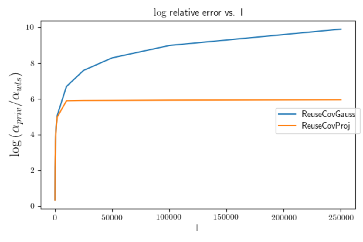
(a) $d=1000,n=5008,(\epsilon,\delta)=(5,\frac{1}{n^{2}}),\lambda=.23$

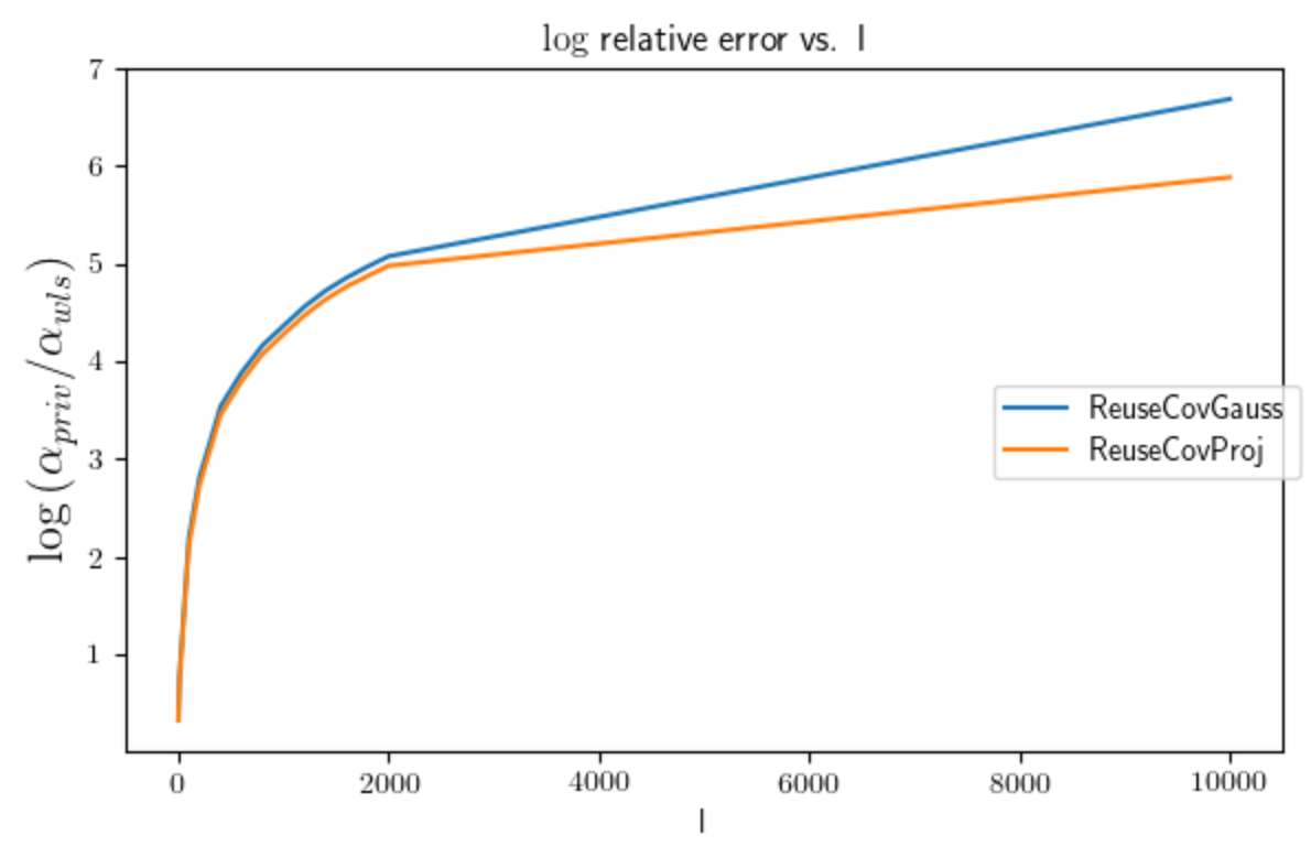
(b) Zoomed in to $l<10000$

Figure 2: Comparing the log of the ratio of the squared loss of the private estimator to the square loss of the OLS estimator, across a range of $l$.

5.2 Results

Setting $(\epsilon,\delta)=(5,\frac{1}{n^{2}})$ with $n=5008$, in Figure 2 we set $d=1000$ and vary $l=(1,11,101,201,401,$ $601,801,1001,1201,1401,1601,1801,2000,10000,$ $25000,50000,100000,250000)$. Each value is averaged over $10$ iterations for each value of $l$. For large $l$, our results our well-supported by the theory; we observe that for $l>2000$ ReuseCovProj begins to noticeably outperform $\texttt{{ReuseCovGauss}},$ and for very large $l$ improves upon ReuseCovGauss by several orders of magnitude. In accordance with Theorem 4.3 for sufficiently large values of $l$ the error of ReuseCovProj has no observable asymptotic dependence on $l$. Interestingly, by zooming into Figure 2(b) we see that the projection still performs as well as ReuseCovGauss even at small values of $l<\frac{n}{\sqrt{d}}$, whereas the analysis would suggest the projection could actually increase error relative to the Gaussian Mechanism in this parameter regime. One practical consequence of these experiments is that it appears the projection does not decrease accuracy even for small values of $l$, and at large values of $l$ achieves a drastic improvement.

6 Appendix

6.1 Additional Related Work

Private release of $2$-way marginals

Consider the problem of privately releasing all $2$-way marginals over $n$ points in $\{0,1\}^{d+l}$. Theorem 5.7 in [30] gives a polynomial time algorithm based on relaxed projections that achieves mean squared error $\tilde{O}(n\sqrt{d+l})$, which matches the best known information theoretic upper bound [30], although there is a small gap to the existing lower bound $\min(n,(d+l)^{2})$. This relaxed projection algorithm outperforms the Gaussian Mechanism when $n\sqrt{d+l}<ld\implies n<\frac{dl}{\sqrt{d+l}}\implies d\sqrt{d+l}>n$. Since the mean squared error of Algorithm 1 that used this projection as a subroutine is at least $\frac{d\sqrt{d+l}}{n}$, this means that in the regime where the projection outperforms the Gaussian Mechanism, we do not achieve mean squared error $<1$ in our regression.

This suggests that, at least using the existing error analysis of SSP from [25], it seems unlikely that by applying specialized algorithms for private release of $2$-way marginals to compute the $\frac{1}{n}X^{T}Y$ term subject to differential privacy in $(X,Y)$, e.g. the label private setting, we can both improve over the Gaussian Mechanism and achieve non-trivial error.

Linear Queries under $l_{\infty}$-loss.

Beyond $2$-way marginals, the problem of privately releasing large numbers of linear queries (Definition 6.1) has been studied extensively. It is known that the worst case error is bounded by $\min(\frac{\sqrt{\log(|\mathcal{Q}|)}(\log|\mathcal{X}|\log(1/\delta))^{1/4}}{\sqrt{n\epsilon}},\frac{\sqrt{|\mathcal{Q}|\log(1/\delta)}}{\epsilon n})$. The first term, which dominates in the so-called low-accuracy or “sparse” ([1]) regime, is achieved by the PrivateMultiplicativeWeights algorithm of [42], which is optimal over worst case workloads [43]. However, this algorithm has running time exponential in the data dimension, which is unavoidable [44] over worst case $\mathcal{Q}$. The second term, which dominates for $n\gg\frac{|\mathcal{Q}|}{\log|\mathcal{Q}|\log|\mathcal{X}|^{1/4}}$, the “high accuracy” regime, is achieved by the simple and efficient Gaussian Mechanism [8], which is also optimal over worst-case sets of queries $\mathcal{Q}$ [43].

Linear Queries under $l_{2}$-loss.

For the $l_{2}$ error, in the high accuracy $n\gg|\mathcal{Q}|$ regime the factorization mechanism achieves error that is exactly tight for any workload of linear queries $\mathcal{Q}$ up to a factor of $\log(1/\delta)$, although it is not efficient (Theorem  [29]). In the low-accuracy regime, the algorithm of [1] that couples careful addition of correlated Gaussian noise (akin to the factorization mechanism) with an $l_{1}$-ball projection step achieves error within log factors of what is (a slight variant) of a quantity known as the hereditary discrepancy $\text{opt}_{\epsilon,\delta}(A,n)$ (Theorem [1]). This quantity is a known lower bound on the error of any $(\epsilon,\delta)$ mechanism for answering linear queries [45], and so the upper bound is tight up to log factors in $|\mathcal{Q}|,|\mathcal{X}|$. Theorem $21$ in [1] analyzes the simple projection mechanism that adds independent Gaussian noise and projects rather than first performing the decomposition step that utilizes correlated Gaussian noise, achieving error $O(nd\log(1/\delta)\sqrt{\log|X|}/\epsilon)$, which matches the best known (worst case over $\mathcal{Q}$) upper bound for the sparse $n<d$ case [46]. In our Theorem 4.2 we give such a universal upper bound, rather than one that depends on the hereditary discrepancy of the matrix $Y$. While the bound can of course be improved for a specific set of outcomes $Y$ by the addition of the decomposition step to the projection algorithm, we omit this step in favor of a simpler algorithm with more directly comparable bounds to existing private regression algorithms.

While the information-theoretic $l_{\infty}$ or $l_{2}$ error achievable for linear queries is well-understood [29, 1, 43], as synthetic data algorithms like PrivateMultiplicativeWeights and MedianMechanism, or the factorization or projection mechanisms are in general inefficient, there are many open problems pertaining to developing efficient algorithms for specific query classes, or heuristic approaches that work better in practice. Examples of these approaches along the lines of the factorization mechanism [47, 48], efficient approximations of the projection mechanism [21, 30], and using heuristic techniques from distribution learning in the framework of iterative synthetic data algorithms [49, 50, 51, 52].

Sub-sampled Linear Regression.

In Subsection 4.4 we analyze SSP where we first sub-sample a random set of $s$ points without replacement, and use this sub-sample to compute the noisy covariance matrix. Sub-sampled linear regression has been studied extensively absent privacy, where it is known that uniform sub-sampling is sub-optimal in that it produces biased estimates of the OLS estimator, and performs poorly in the presence of high-leverage points [53]. To address these shortcomings, techniques based on leverage score sampling [54], volume-based sampling [55][53], and spectral sparsification [56] have been developed. Crucially, in these methods the probability of a point being sub-sampled is data-dependent, and so they are (not obviously) compatible with differential privacy.

6.2 Lemmas and Definitions

Throughout the paper we make heavy use of common matrix and vector norms. For a vector $v\in\mathbb{R}^{d}$ and matrix $A\in\mathbb{R}^{d\times d},||v||_{A}^{2}\vcentcolon=v^{t}Av,||A||_{2}^{2}=\lambda_{\max}(A^{T}A),||v||_{2}^{2}=\sum_{k=1}^{d}v_{k}^{2},||A||_{F}^{2}=\sum_{i,j\in[d]}a_{ij}^{2}$.

Definition 6.1.

Statistical Query [57] Let $D\in\mathcal{X}^{n}$ a dataset. A linear query is a function $q:\mathcal{X}\to[0,1]$, where $q(D)\vcentcolon=\frac{1}{n}\sum_{x_{i}\in D}^{n}q(x_{i})$.

Definition 6.2.

[58] Let $\mathcal{X}=\{0,1\}^{m}$, and $\mathcal{Q}_{k}=\{q_{ij}\}_{1\leq i_{1}<i_{2}<i_{k}\leq m},$ where $q_{ij}(x)\vcentcolon=\prod_{u=1}^{k}x_{i_{u}}$. Then the class $\mathcal{Q}_{k}$ are called $k-$way marginals.

Lemma 6.

[41] Let $Z_{i}\in\mathbb{S}_{d}^{+}$, and sample $Z_{1},\ldots Z_{s}$ without replacement from $\{Z_{1},\ldots Z_{n}\}$. Suppose $\mathbb{E}[Z_{i}]=I_{d}$, and $\max_{i\in[n]}\lambda_{\max}(Z_{i})\leq B$. Then for $\delta=\sqrt{\frac{2B\log(2d/\rho)}{s}}$, with probability $1-\rho$:

$$\lambda_{\max}(\frac{1}{s}\sum_{i=1}^{s}Z_{i})<1+\delta,\;\;\lambda_{\min}(\frac{1}{s}\sum_{i=1}^{s}Z_{i})>1-\delta$$

Lemma 7 (folklore e.g. [59]).

Given a dataset $\mathcal{X}^{n}$ of $n$ points and an $(\epsilon,\delta)-$DP mechanism $M$. Let the procedure subsample take a random subset of $s$ points from $\mathcal{X}^{n}$ without replacement. Then if $\gamma=s/n$, the procedure $M\circ\textbf{subsample}$ is $(O(\gamma\epsilon),\gamma\delta)-$DP for sufficiently small $\epsilon$.

6.3 Proofs from Subsection 4.1

The following lemma is used repeatedly in analyzing the accuracy of all $SSP$ variants.

Lemma 8.

Let $A,B$ invertible matrices in $\mathbb{R}^{n\times n}$, and $v,c$ vectors $\in\mathbb{R}^{n}$.

Then

$$A^{-1}v-(A+B)^{-1}(v+c)=(A+B)^{-1}BA^{-1}v-(A+B)^{-1}c$$

Proof.

Expanding we get that:

$$A^{-1}v-(A+B)^{-1}(v+c)=(A^{-1}-(A+B)^{-1})v-(A+B)^{-1}c,$$

so it suffices to show that:

$$(A^{-1}-(A+B)^{-1})v=(A+B)^{-1}BA^{-1}v$$

Now the Woodbury formula tells us that $(A+B)^{-1}=A^{-1}-(A+AB^{-1}A)^{-1},$ hence

$$(A^{-1}-(A+B)^{-1})v=(A+AB^{-1}A)^{-1}v=(A(I+B^{-1}A))^{-1}v$$

Then since:

$$(A(I+B^{-1}A))^{-1}=(I+B^{-1}A)^{-1}A^{-1}=(B^{-1}(B+A))^{-1A^{-1}}=(B+A)^{-1}BA^{-1},$$

we are done. ∎

Proof of $(\epsilon,\delta)$-DP in Theorem 4.1:

Proof.

The privacy proof follows from a straightforward application of the Gaussian mechanism. We note that releasing each $\hat{v}_{i}$ privately, is equivalent to computing $X^{T}Y+E_{2}$, where $E_{2}\sim N_{d\times l}(0,\sigma_{2}^{2})$. Now it is easy to compute $l$-sensitivity $\Delta(f)$ of $f(X)=X^{T}Y$. Fix an individual $i$, and an adjacent dataset $X^{\prime}=X/\{x_{i},y_{i}\}\cup\{x_{i}^{\prime},y_{i}^{\prime}\}$. Then $f(X)-f(X^{\prime})=\Delta_{V}=[y_{i1}x_{i}-y_{i1}^{\prime}x_{i1}^{\prime},\ldots y_{il}x_{i}-y_{il}^{\prime}x_{il}^{\prime}]$. Then:

$$||f(X)-f(X^{\prime})||=\sqrt{||\Delta_{V}||^{2}_{F}}=\sqrt{\sum_{j=1}^{l}||y_{ij}x_{i}-y_{ij}^{\prime}x_{ij}^{\prime}||^{2}}\leq\sqrt{l\cdot 4||\mathcal{X}||^{2}||\mathcal{Y}||^{2}}=2\sqrt{l}||\mathcal{X}||||\mathcal{Y}||$$

Hence setting $\sigma_{2}=c(\epsilon,\delta)2\sqrt{l}||\mathcal{X}||||\mathcal{Y}||/\epsilon$ by the Gaussian mechanism [8] publishing $\hat{V}$ satisfies $(\epsilon/2,\delta/2)-DP$. Similarly if $g=X^{T}X$, $\Delta(g)\leq||X||^{2}$, and so setting $\sigma_{1}=c(\epsilon,\delta)||X||^{2}/\epsilon$, means publishing $\hat{I}$ is $(\epsilon/2,\delta/2)$-DP. By basic composition for DP, the entire mechanism is $(\epsilon,\delta)$-DP. ∎

Proof of Accuracy in Theorem 4.1:

Proof.

We follow the general proof technique developed in [25] analysing the accuracy guarantees of the ridge regression variant of SSP in the case $\lambda_{\min}(X^{T}X)=0$, adding some mathematical detail to their exposition, and doing the appropriate book-keeping to handle our setting where the privacy level (as a function of the noise level) guaranteed by $E_{1}$ and $E_{2}$ differ. The reader less interested in these details can skip to Equation 25 below for the punchline.

Fix a specific index $i\in[l]$, and let $y=y_{i}$. We will analyze the prediction error of $\hat{w_{i}}$ e.g. $F(w_{i})-F(w_{i}^{*})$. Then the following result is stated in [25] for which provide a short proof:

Lemma 9.

$$F(\hat{w_{i}})-F(w_{i*})=||y-X\hat{w_{i}}||^{2}-||y-Xw_{i*}||=||\hat{w_{i}}-w_{i*}||^{2}_{X^{T}X}$$

Proof.

We note that all derivatives of orders higher than $2$ of $f(w)=||y-Xw||^{2}$ are zero, and that $\nabla f_{w_{i*}}=0$ by the optimality of $w_{i*}$. We also note that the Hessian $\nabla^{2}f_{w}=X^{T}X$ at all points $w$. Then by the Taylor expansion of $f(w)$ around $w_{i*}$:

$$f(\hat{w_{i}})=f(w_{i*})+(\hat{w_{i}}-w_{i*})\cdot\nabla f_{w_{i*}}+(\hat{w_{i}}-w_{i*})^{\prime}X^{T}X(\hat{w_{i}}-w_{i*})$$

Which using $\nabla f_{w_{i*}}=0$ and rearranging terms gives the result. ∎

Now Corollary 7 in the Appendix of [25] states (without proof) the below identity, which we provide a proof of for completeness via Lemma 8:

$$\hat{w_{i}}-w_{i*}=(-X^{T}X+\lambda I+E_{1})^{-1}E_{1}w_{i*}-\lambda(X^{T}X+\lambda I+E_{1})^{-1}w_{i*}+(X^{T}X+\lambda I+E_{1})^{-1}E_{2}$$ (21)

Hence, still following [25], for any psd matrix $A$, $||\hat{w_{i}}-w_{i*}||_{A}^{2}\leq$

$$3||(X^{T}X+\lambda I+E_{1})^{-1}E_{1}w_{i*}||_{A}^{2}+3\lambda^{2}||(X^{T}X+\lambda I+E_{1})^{-1}w_{i*}||_{A}^{2}+3||(X^{T}X+\lambda I+E_{1})^{-1}E_{2}||_{A}^{2}$$ (22)

Lemma 10.

[25] With probability $1-\rho$, $||E_{1}||\leq(\lambda_{\min}(X^{T}X)+\lambda)/2$, and hence

$$X^{T}X+\lambda I+E_{1}\succ.5(X^{T}X+\lambda I)$$

We also remark that $||By||_{A}^{2}=(By)^{T}ABy=||y||_{B^{T}AB}^{2}$ for any vector $y$, and matrices $A,B$.

Hence, Inequality 22, with $A=X^{T}X$ can be further simplified to:

$$3||(X^{T}X+\lambda I+E_{1})^{-1}E_{1}w_{i*}||_{A}^{2}+3\lambda^{2}||(X^{T}X+\lambda I+E_{1})^{-1}w_{i*}||_{A}^{2}+3||(X^{T}X+\lambda I+E_{1})^{-1}E_{2}||_{A}^{2}\leq\\ O\left(||E_{1}w_{i*}||_{(X^{T}X+\lambda I+E_{1})^{-1}}^{2}+\lambda^{2}||w_{i*}||_{(X^{T}X+\lambda I+E_{1})^{-1}}^{2}+||E_{2}||^{2}_{(X^{T}X+\lambda I+E_{1})^{-1}}\right)\leq\\ \text{(Lemma~{}\ref{matrixneq})}\;\;O\left(||E_{1}w_{i*}||_{(X^{T}X+\lambda I)^{-1}}^{2}+\lambda^{2}||w_{i*}||_{(X^{T}X+\lambda I)^{-1}}^{2}+||E_{2}||^{2}_{(X^{T}X+\lambda I)^{-1}}\right)$$ (23)

By basic properties of the trace we have: $\text{tr}(({\lambda I+X^{T}X)^{-1}})\leq d\lambda_{max}({\lambda I+X^{T}X^{-1}})=\frac{d}{\lambda_{\min}(\lambda I+X^{T}X)}=\frac{d}{(\lambda_{\min}+\lambda)}$, and $||w_{i*}||_{(X^{T}X+\lambda I)^{-1}}^{2}\leq\frac{||w_{i*}||^{2}}{\lambda}$. Continuing from [25] by their Lemma 6, we can bound each $||E_{1}w_{i*}||_{(X^{T}X+\lambda I)^{-1}}^{2}$ and $||E_{2}||^{2}_{(X^{T}X+\lambda I)^{-1}}$.

Lemma 11 ([25]).

Let $\theta\in\mathbb{R}^{d}$ and let $E$ a symmetric Gaussian matrix where the upper triangular region is sampled from $N(0,\sigma^{2})$ and let $A$ be any psd matrix. Then with probability $1-\rho$:

$$||E\theta||_{A}^{2}\leq\sigma^{2}\text{tr}(A)||\theta||^{2}\log(2d^{2}/\rho)$$

Then recalling that:

• $\sigma_{1}^{2}=\tilde{O}(||\mathcal{X}||^{4}/\epsilon^{2})$

• $\sigma_{2}^{2}=\tilde{O}(l||\mathcal{X}||^{2}|\mathcal{Y}|^{2}/\epsilon^{2})$

Plugging into Lemma 11, and bringing it all together we get:

$$|F(\hat{w_{i}})-F(w_{i*})|\leq||w_{i*}-\hat{w_{i}}||_{X^{T}X}=\\ O\left(||E_{1}w_{i*}||_{(X^{T}X+\lambda I)^{-1}}^{2}+\lambda^{2}||w_{i*}||_{(X^{T}X+\lambda I)^{-1}}^{2}+||E_{2}||^{2}_{(X^{T}X+\lambda I)^{-1}}\right)=\\ \tilde{O}\left(\frac{d}{\lambda_{\min}+\lambda}||w_{i*}||^{2}(||\mathcal{X}||^{4}/\epsilon^{2})\log(2d^{2}/\rho)+\lambda||w_{i*}||^{2}+\frac{d}{\lambda_{\min}+\lambda}l||\mathcal{X}||^{2}|\mathcal{Y}|^{2}/\epsilon^{2}\log(2d^{2}/\rho)\right)$$ (24)

Upper bounding Equation 24 by taking $\lambda_{\min}=0$, we minimize over $\lambda$ setting

$$\lambda=\tilde{O}\left(\frac{1}{\epsilon}\sqrt{d\log(2d^{2}/\rho)}||X||\sqrt{||\mathcal{X}||^{2}+\frac{l|\mathcal{Y}|^{2}}{||w_{i*}||^{2}}}\right)\implies\\ |F(\hat{w_{i}})-F(w_{i*})|=\tilde{O}\left(\frac{1}{\epsilon}\sqrt{d\log(2d^{2}/\rho)}||X||\sqrt{||\mathcal{X}||^{2}||w_{i*}||^{4}+l|\mathcal{Y}|^{2}||w_{i*}||^{2}}\right)$$ (25)

Now if we are in the $\eta-$small regime, we have $|\mathcal{Y}|\leq\eta||\mathcal{X}||||w_{i*}||$, and so

$$l|\mathcal{Y}|^{2}w_{i*}^{2}\leq l\eta^{2}{||\mathcal{X}||}^{2}{||w_{i*}||}^{4},$$

which reduces Equation 25 to:

$$|F(\hat{w_{i}})-F(w_{i*})|=\tilde{O}\left(\frac{1}{\epsilon}\sqrt{d\log(2d^{2}/\rho)}||X||^{2}||w_{i*}||^{2}(\eta\sqrt{l})\right),$$

as desired. ∎

Proof of Theorem 4.3

Proof.

We start with our usual expansion of $f(\hat{w_{i}})-f(w_{i*})$, up until Equation 24, we have with probability $1-\rho$ for every $i\in[l]$:

$$n\cdot f(\hat{w_{i}})-f(w_{i*})=\tilde{O}\left(\frac{d}{\lambda_{\min}+\lambda}||w_{i*}||^{2}(||\mathcal{X}||^{4}/\epsilon^{2})\log(2d^{2}/\rho)+\lambda||w_{i*}||^{2}+\frac{1}{\lambda_{\min}+\lambda}||E_{2i}||^{2}_{2}\right)$$ (26)

Aggregating over $i$ and rearranging gives:

$$\frac{n}{l}\sum_{i=1}^{l}f(\hat{w_{i}})-f(w_{i*})=\tilde{O}\left(\frac{d}{\lambda_{\min}+\lambda}||\hat{w}||^{2}(||\mathcal{X}||^{4}/\epsilon^{2})\log(2d^{2}/\rho)+\lambda||\hat{w}||^{2}+\frac{1}{\lambda_{\min}+\lambda}\frac{1}{l}\sum_{i=1}^{l}||E_{2i}||^{2}_{2}\right),$$ (27)

where $||\hat{w}||^{2}=\frac{1}{l}\sum_{i=1}^{l}||w_{i*}||^{2}=\frac{1}{l}||W^{*}||_{F}^{2}$. Then by Theorem 4.2, we have with $\frac{1}{l}\sum_{i=1}^{l}||E_{2i}||^{2}_{2}=O\left(c(\epsilon,\delta)\sqrt{\log(2/\rho)}n\sqrt{d}|\mathcal{Y}|^{2}||\mathcal{X}||^{2}\right)$ with probability $1-\rho$. So with probability $1-2\rho$, we have $\frac{n}{l}\sum_{i=1}^{l}f(\hat{w_{i}})-f(w_{i*})=$

$$\tilde{O}\left(\frac{d}{\lambda_{\min}+\lambda}||\hat{w}||^{2}(||\mathcal{X}||^{4}/\epsilon^{2})\log(2d^{2}/\rho)+\lambda||\hat{w}||^{2}+\frac{1}{\lambda_{\min}+\lambda}c(\epsilon,\delta)\sqrt{\log(2/\rho)}n\sqrt{d}|\mathcal{Y}|^{2}||\mathcal{X}||^{2}\right)$$ (28)

Finally optimizing over $\lambda$ gives the desired result:

$$\alpha=\tilde{O}\left(||\hat{w}||\sqrt{\frac{d||\hat{w}||^{2}(||\mathcal{X}||^{4}/\epsilon^{2})\log(2d^{2}/\rho)}{n^{2}}+\frac{c(\epsilon,\delta)\sqrt{\log(2/\rho)}\sqrt{d}|\mathcal{Y}|^{2}||\mathcal{X}||^{2}}{n}}\right)$$

∎

6.4 Proofs from Subsection 4.4

Proof of Theorem Theorem:

Proof.

Our analysis will hinge on the case where $l=1$ e.g. that of standard private linear regression, which we will extend to the PRIMO case by our choice of $\epsilon$ as in the proof of Theorem 4.1. The fact that the Algorithm is $(O(\epsilon),\delta)$ private follows immediately from the Gaussian mechanism, and the secrecy of the sub-sample lemma (Lemma 7), which is why we can set $\epsilon_{1}=\frac{n}{s}\epsilon/2$ in Line $2$. We proceed with the accuracy analysis.

Define:

• $w_{i*}=(X^{T}X)^{-1}X^{T}Y$: the least squares estimator as before

• $w_{i*}^{\lambda}=(\frac{1}{n}X^{T}X+\lambda I)^{-1}\frac{1}{n}X^{T}Y$: the ridge regression estimator

• $w_{s}=(\frac{1}{s}X_{S}^{T}X_{S}+\lambda I)^{-1}(\frac{1}{n}X^{T}Y)$: the sub-sampled least squares estimator

• $\tilde{w}_{s}=(\frac{1}{s}X_{S}^{T}X_{S}+E_{1}+\lambda I)^{-1}(\frac{1}{n}X^{T}Y+E_{2})$: differentially private estimate of $w_{s}$

We note that $0\leq f(w_{i*}^{\lambda})-f(w_{i*})\leq\lambda\left(||w_{i*}||^{2}-||w_{i*}^{\lambda}||^{2}\right)\leq\lambda||\mathcal{W}||^{2}$. Then by the Lemma  9 and Cauchy-Schwartz with respect to the norm $||\cdot||_{\frac{X^{T}X}{n}}$:

$$|f(\tilde{w}_{s})-f(w_{i*})|=||\tilde{w}_{s}-w_{i*}||_{\frac{X^{T}X}{n}}^{2}\leq\\ 3||w_{i*}-w_{i*}^{\lambda}||_{\frac{X^{T}X}{n}}^{2}+3||w_{i*}^{\lambda}-w_{s}||_{\frac{X^{T}X}{n}}^{2}+3||w_{s}-\tilde{w}_{s}||_{\frac{X^{T}X}{n}}^{2}\leq\\ 3\lambda||\mathcal{W}||^{2}+3||w_{s}-w_{i*}^{\lambda}||_{\frac{X^{T}X}{n}}^{2}+3||\tilde{w}_{s}-w_{s}||_{\frac{X^{T}X}{n}}^{2}$$ (29)

Lemmas 12, 13 bound these terms with high probability.

Lemma 12.

Under the assumption $||\mathcal{X}||=O(n\lambda)$, then w.p. $1-\rho/2$:

$$||w_{i*}^{\lambda}-w_{s}||_{\frac{X^{T}X}{n}}=O\left(\frac{||\mathcal{X}|||\mathcal{Y}|\log(2d/\rho)}{\lambda s}\right)$$

Lemma 13.

Under the assumption $||\mathcal{X}||=O(n\lambda)$, then w.p. $1-\rho/2$:

$$||w_{s}-\tilde{w}_{s}||_{\frac{X^{T}X}{n}}=O(\frac{||X||^{4}}{n^{2}\epsilon^{2}}||\mathcal{W}||^{2}\cdot\frac{d}{\lambda}\frac{\log(2d/\rho)}{s}+\frac{l||\mathcal{X}||^{2}||\mathcal{Y}||^{2}}{n^{2}\epsilon^{2}}\cdot\frac{d}{\lambda}\frac{\log(2d/\rho)}{s})$$ (30)

Then by Equation 29 and Lemmas 12, 13, we get that w.p. $1-\rho$:

$$f(\tilde{w}_{s})-f(w_{i*})=\\ O\left(\lambda||w_{i*}||^{2}+\frac{||\mathcal{X}|||\mathcal{Y}|}{\lambda}(\frac{\log(2d/\rho)}{s})+\frac{||X||^{4}n^{2}}{s^{4}\epsilon^{2}}||\mathcal{W}||^{2}\cdot\frac{d}{\lambda}(1+\frac{\log(2d/\rho)}{s})\;+\;\frac{l||\mathcal{X}||^{2}||\mathcal{Y}||^{2}}{n^{2}\epsilon^{2}}\cdot\frac{d}{\lambda}(1+\frac{\log(2d/\rho)}{s})\right),$$ (31)

Summing over $i$ and minimizing over $\lambda$ we set

$$\lambda=\frac{\sqrt{||\mathcal{X}|||\mathcal{Y}|(\frac{\log(2d/\rho)}{s})+\frac{||X||^{4}n^{2}}{s^{4}\epsilon^{2}}||\mathcal{W}||^{2}\cdot\frac{d}{\lambda}(1+\frac{\log(2d/\rho)}{s})\;+\;\frac{l||\mathcal{X}||^{2}||\mathcal{Y}||^{2}}{n^{2}\epsilon^{2}}\cdot\frac{d}{\lambda}(1+\frac{\log(2d/\rho)}{s})}}{\sqrt{1}{l}||W||_{F}},$$

which completes the result. ∎

Proof of Lemma 12:

Proof.

Now:

$$||w_{i*}^{\lambda}-w_{s}||_{\frac{1}{n}X^{T}X}^{2}=n||w_{i*}^{\lambda}-w_{s}||_{\frac{1}{n}X^{T}X}^{2}\leq n||w_{i*}^{\lambda}-w_{s}||_{\frac{1}{n}X^{T}X+\lambda I}^{2}$$

We will focus on $||w_{i*}^{\lambda}-w_{s}||_{\frac{1}{n}X^{T}X+\lambda I}^{2}$. Let $\Sigma=\frac{1}{n}X^{T}X+\lambda I$, $\Sigma_{s}=\frac{1}{s}\sum_{j\in S}x_{s}x_{s}^{T}+\lambda I$, and $v=\frac{1}{n}X^{T}Y$. Expanding $||w_{i*}^{\lambda}-w_{s}||_{\Sigma}=$

$$(\Sigma_{s}^{-1}v-\Sigma^{-1}v)^{T}\Sigma(\Sigma_{s}^{-1}v-\Sigma^{-1}v)=v^{T}\overbrace{(\Sigma_{s}^{-1}-\Sigma^{-1})\Sigma(\Sigma_{s}^{-1}-\Sigma^{-1})}^{A}v=v^{T}Av$$ (32)

Now since $A$ is Hermitian, we know $||v||_{A}\leq||v||||A||_{2}$. Since $||v||\leq||\mathcal{X}|||\mathcal{Y}|$, it suffices to bound $||A||_{2}$ with high probability. Noting that $A=(\Sigma_{s}^{-1}-\Sigma^{-1})\Sigma(\Sigma_{s}^{-1}-\Sigma^{-1})=\Sigma_{s}^{-1}\Sigma^{1/2}(I-\Sigma^{-1/2}\Sigma_{s}\Sigma^{-1/2})(I-\Sigma^{-1/2}\Sigma_{s}\Sigma^{-1/2})\Sigma^{1/2}\Sigma_{s}^{-1}$, we have by the sub-multiplicativity of the operator norm:

$$||A||_{2}\leq\left(||\Sigma_{S}^{-1}\Sigma^{1/2}||_{2}^{2}\right)\cdot\left(||I-\Sigma^{-1/2}\Sigma_{s}\Sigma^{-1/2}||_{2}^{2}\right)\leq\\ \frac{\lambda_{\max}(\Sigma)}{\lambda^{2}}\cdot\left(||I-\Sigma^{-1/2}\Sigma_{s}\Sigma^{-1/2}||_{2}^{2}\right)$$ (33)

Now consider $\Sigma^{-1/2}\Sigma_{s}\Sigma^{-1/2}=\Sigma^{-1/2}\frac{1}{s}\sum_{j\in S}(x_{s}x_{s}^{T}+\lambda I)\Sigma^{-1/2}=\frac{1}{s}\sum_{j\in s}Z_{i}$. Then note that $\mathbb{E}[Z_{i}]=\Sigma^{-1/2}(\frac{1}{n}\mathbb{E}[x_{i}x_{i}^{T}]+\lambda I)\Sigma^{-1/2}=\Sigma^{-1/2}\Sigma\Sigma^{-1/2}=I$, and that $\lambda_{max}(Z_{i})\leq||\Sigma^{-1}||_{2}||\frac{1}{n}x_{i}x_{i}^{T}+\lambda I||_{2}\leq 1+\frac{||\mathcal{X}||}{n\lambda}$.

Now we can bound $||I-\frac{1}{s}\sum_{j\in s}Z_{i}||_{2}$ by Theorem 2.2 in [41]:

Lemma 14.

[41] Let $Z_{1},\ldots Z_{s}$ sampled without replacement from $\{Z_{1},\ldots Z_{n}\}$. Then if $Z_{i}\in\mathbb{S}_{d}^{+},\mathbb{E}[Z_{i}]=I_{d}$, and $\max_{i\in[n]}\lambda_{\max}(Z_{i})\leq B$ w.p. $1-\rho$, for $\delta=\sqrt{\frac{2B\log(2d/\rho)}{s}}$:

$$\lambda_{\max}(\frac{1}{s}\sum_{i=1}^{s}Z_{i})<1+\delta,\;\;\lambda_{\min}(\frac{1}{s}\sum_{i=1}^{s}Z_{i})>1-\delta$$

So by Lemma 14, we know that with probability $1-\rho$: $|\lambda_{\min}(I-\Sigma^{-1/2}\Sigma_{s}\Sigma^{-1/2})|=1-\lambda_{\max}(\Sigma^{-1/2}\Sigma_{s}\Sigma^{-1/2})\leq\delta$, and similarly $|\lambda_{\max}(I-\Sigma^{-1/2}\Sigma_{s}\Sigma^{-1/2})|\leq\delta$, thus $||I-\Sigma^{-1/2}\Sigma_{s}\Sigma^{-1/2})||_{2}\leq\delta$. Substituting this all into Equation 33 and noting $\lambda_{\max}(\Sigma)\leq\frac{||\mathcal{X}||}{n}+\lambda$ we get with probability $1-\rho$:

$$||w_{i*}^{\lambda}-w_{s}||_{\frac{1}{n}X^{T}X}\leq||\tilde{w}_{s}-w_{s}||_{\Sigma}\leq||\mathcal{X}|||\mathcal{Y}|n||A||_{2}\leq||\mathcal{X}||||Y||\frac{\lambda_{\max}(\Sigma)}{\lambda^{2}}\delta^{2}=$$ (34)

$$2||\mathcal{X}|||\mathcal{Y}|\frac{(\frac{||\mathcal{X}||}{n}+\lambda)^{2}}{\lambda^{3}}\frac{\log(2d/\rho)}{s},$$ (35)

which under the assumption $||\mathcal{X}||=O(n\lambda)$ gives $O(\frac{||\mathcal{X}|||\mathcal{Y}|\log(2d/\rho)}{\lambda s})$. as desired. ∎

Proof of Lemma 13:

Proof.

By Lemma 8, with $A=\frac{1}{s}X_{S}^{T}X+\lambda I$, $B=E_{1},c=E_{2},v=\frac{1}{n}^{T}Y$, we get $w_{s}-\tilde{w}_{s}=(\frac{1}{s}X_{S}^{T}X+\lambda I+E_{1})E_{1}w_{s}-(\frac{1}{s}X_{S}^{T}X+\lambda I+E_{1})^{-1}E_{2}$, and so

$$||w_{s}-\tilde{w}_{s}||_{\frac{X^{T}X}{n}}^{2}\leq 2||(\frac{1}{s}X_{S}^{T}X+\lambda I+E_{1})^{-1}E_{1}w_{s}||_{\frac{X^{T}X}{n}}^{2}+2||(\frac{1}{s}X_{S}^{T}X+\lambda I+E_{1})^{-1}E_{2}||_{\frac{X^{T}X}{n}}^{2}$$

Under the assumption $||E_{1}||_{2}\leq\lambda/2,$ this becomes

$$||w_{s}-\tilde{w}_{s}||_{\frac{X^{T}X}{n}}^{2}=O\left(||E_{1}w_{s}||_{(\frac{1}{s}X_{S}^{T}X_{S}+\lambda I)^{-1}(X^{T}X/n+\lambda I)(\frac{1}{s}X_{S}^{T}X_{S}+\lambda I)^{-1}}\right)+\\ O\left(||E_{2}||_{(\frac{1}{s}X_{S}^{T}X_{S}+\lambda I)^{-1}(X^{T}X/n+\lambda I)(\frac{1}{s}X_{S}^{T}X_{S}+\lambda I)^{-1}}\right)$$ (36)

Now to apply Lemma 11, we need to bound

$$\text{Tr}((\frac{1}{s}X_{S}^{T}X_{S}+\lambda I)^{-1}(X^{T}X/n+\lambda I)(\frac{1}{s}X_{S}^{T}X_{S}+\lambda I)^{-1})\leq d\lambda_{\max}(\Sigma_{S})^{-1}(\Sigma)(\Sigma_{S})^{-1})=\\ d\lambda_{\max}(\Sigma^{-1/2}(\Sigma^{1/2}\Sigma_{S}^{-1}\Sigma^{1/2})^{2}\Sigma^{-1/2})\leq\\ d\lambda_{\max}(\Sigma^{-1})\frac{1}{\lambda_{\min}(\Sigma^{-1/2}\Sigma^{1/2}\Sigma_{S}^{-1}\Sigma^{1/2})}^{2}\leq\frac{d}{\lambda}(\frac{1}{1-\delta})^{2},$$ (37)

where the last inequality follows from Lemma 14. Applying Lemma 11 we get that with probability $1-2\rho$:

$$||w_{i*}^{\lambda}-w_{s}||_{X^{T}X/n}=O\left(\sigma_{1}^{2}\cdot\frac{d}{\lambda}(\frac{1}{1-\delta})^{2}\cdot||w_{s}||^{2}\log(2d^{2}/\rho)+\sigma_{2}^{2}\cdot\frac{d}{\lambda}(\frac{1}{1-\delta})^{2}\log(2d^{2}/\rho)\right),$$ (38)

From Lemma 14, $\delta=\sqrt{\frac{2(1+\frac{||\mathcal{X}||}{n\lambda})\log(2d/\rho)}{s}}$, which under the assumption $||\mathcal{X}||=O\left(n\lambda\right)$ gives $\frac{1}{(1-\delta)}^{2}=O(1+\frac{\log(2d/\rho)}{s})^{2}$. Substituting in the value of $\sigma_{1},\sigma_{2}$ gives:

$$\frac{||X||^{4}n^{2}}{s^{4}\epsilon^{2}}||\mathcal{W}||^{2}\cdot\frac{d}{\lambda}(1+\frac{\log(2d/\rho)}{s})\;+\;\frac{l||\mathcal{X}||^{2}||\mathcal{Y}||^{2}}{n^{2}\epsilon^{2}}\cdot\frac{d}{\lambda}(1+\frac{\log(2d/\rho)}{s}),$$

as desired. ∎

References

- [1] Aleksandar Nikolov, Kunal Talwar, and Li Zhang. The geometry of differential privacy: the sparse and approximate cases. In STOC ’13, 2013.
- [2] E. Krapohl, H. Patel, S. Newhouse, C J Curtis, S. von Stumm, P S Dale, D. Zabaneh, G. Breen, P F O’Reilly, and R. Plomin. Multi-polygenic score approach to trait prediction. Molecular Psychiatry, 23(5):1368–1374, 2018.
- [3] Jack Pattee and Wei Pan. Penalized regression and model selection methods for polygenic scores on summary statistics. PLOS Computational Biology, 16(10):1–27, 10 2020.
- [4] Alanz Agresti and Barbara Finlay. Statistical methods for the social sciences. Pearson Prentice Hall, 2009.
- [5] Nils Homer, Szabolcs Szelinger, Margot Redman, David Duggan, Waibhav Tembe, Jill Muehling, John V. Pearson, Dietrich A. Stephan, Stanley F. Nelson, and David W. Craig. Resolving individuals contributing trace amounts of dna to highly complex mixtures using high-density snp genotyping microarrays. PLOS Genetics, 4(8):1–9, 08 2008.
- [6] Hongsheng Hu, Zoran Salcic, Lichao Sun, Gillian Dobbie, Philip S Yu, and Xuyun Zhang. Membership inference attacks on machine learning: A survey. ACM Computing Surveys (CSUR), 2021.
- [7] Reza Shokri, Marco Stronati, and Vitaly Shmatikov. Membership inference attacks against machine learning models. CoRR, abs/1610.05820, 2016.
- [8] Cynthia Dwork and Aaron Roth. The algorithmic foundations of differential privacy. Foundations and Trends in Theoretical Computer Science, 9(3-4):211–407, 2014.
- [9] Andrew Gelman and Eric Loken. The statistical crisis in science. 102:460+.
- [10] Cynthia Dwork, Vitaly Feldman, Moritz Hardt, Toniann Pitassi, Omer Reingold, and Aaron Roth. Generalization in adaptive data analysis and holdout reuse. CoRR, abs/1506.02629, 2015.
- [11] Raef Bassily, Kobbi Nissim, Adam D. Smith, Thomas Steinke, Uri Stemmer, and Jonathan R. Ullman. Algorithmic stability for adaptive data analysis. CoRR, abs/1511.02513, 2015.
- [12] Keegan Korthauer, Patrick K. Kimes, Claire Duvallet, Alejandro Reyes, Ayshwarya Subramanian, Mingxiang Teng, Chinmay Shukla, Eric J. Alm, and Stephanie C. Hicks. A practical guide to methods controlling false discoveries in computational biology. Genome Biology, 20(1):118, 2019.
- [13] Jonathan R. Ullman. Private multiplicative weights beyond linear queries. CoRR, abs/1407.1571, 2014.
- [14] Susan Fairley, Ernesto Lowy-Gallego, Emily Perry, and Paul Flicek. The International Genome Sample Resource (IGSR) collection of open human genomic variation resources. Nucleic Acids Research, 48(D1):D941–D947, 10 2019.
- [15] Badih Ghazi, Noah Golowich, Ravi Kumar, Pasin Manurangsi, and Chiyuan Zhang. On deep learning with label differential privacy. CoRR, abs/2102.06062, 2021.
- [16] Hossein Esfandiari, Vahab S. Mirrokni, Umar Syed, and Sergei Vassilvitskii. Label differential privacy via clustering. CoRR, abs/2110.02159, 2021.
- [17] Nicolas Papernot, Martín Abadi, Úlfar Erlingsson, Ian Goodfellow, and Kunal Talwar. Semi-supervised knowledge transfer for deep learning from private training data, 2016.
- [18] Raef Bassily, Adam D. Smith, and Abhradeep Thakurta. Private empirical risk minimization, revisited. CoRR, abs/1405.7085, 2014.
- [19] Duy Vu and Aleksandra Slavkovic. Differential privacy for clinical trial data: Preliminary evaluations. In 2009 IEEE International Conference on Data Mining Workshops, pages 138–143, 2009.
- [20] James R. Foulds, Joseph Geumlek, Max Welling, and Kamalika Chaudhuri. On the theory and practice of privacy-preserving bayesian data analysis. CoRR, abs/1603.07294, 2016.
- [21] Sergül Aydöre, William Brown, Michael Kearns, Krishnaram Kenthapadi, Luca Melis, Aaron Roth, and Ankit A. Siva. Differentially private query release through adaptive projection. CoRR, abs/2103.06641, 2021.
- [22] Cynthia Dwork, Krishnaram Kenthapadi, Frank McSherry, Ilya Mironov, and Moni Naor. Our data, ourselves: Privacy via distributed noise generation. In Serge Vaudenay, editor, Advances in Cryptology - EUROCRYPT 2006, 25th Annual International Conference on the Theory and Applications of Cryptographic Techniques, St. Petersburg, Russia, May 28 - June 1, 2006, Proceedings, volume 4004 of Lecture Notes in Computer Science, pages 486–503. Springer, 2006.
- [23] Ilya Mironov. Renyi differential privacy. CoRR, abs/1702.07476, 2017.
- [24] Jason Milionis, Alkis Kalavasis, Dimitris Fotakis, and Stratis Ioannidis. Differentially private regression with unbounded covariates. In Gustau Camps-Valls, Francisco J. R. Ruiz, and Isabel Valera, editors, Proceedings of The 25th International Conference on Artificial Intelligence and Statistics, volume 151 of Proceedings of Machine Learning Research, pages 3242–3273. PMLR, 28–30 Mar 2022.
- [25] Yu-Xiang Wang. Revisiting differentially private linear regression: optimal and adaptive prediction and estimation in unbounded domain, 2018.
- [26] Daniel Kifer, Adam Smith, and Abhradeep Thakurta. Private convex empirical risk minimization and high-dimensional regression. In Shie Mannor, Nathan Srebro, and Robert C. Williamson, editors, Proceedings of the 25th Annual Conference on Learning Theory, volume 23 of Proceedings of Machine Learning Research, pages 25.1–25.40, Edinburgh, Scotland, 25–27 Jun 2012. PMLR.
- [27] Christos Dimitrakakis, Blaine Nelson, Zuhe Zhang, Aikaterini Mitrokotsa, and Benjamin Rubinstein. Bayesian differential privacy through posterior sampling, 2013.
- [28] Kamalika Chaudhuri, Claire Monteleoni, and Anand D. Sarwate. Differentially private empirical risk minimization. Journal of Machine Learning Research, 12(29):1069–1109, 2011.
- [29] Alexander Edmonds, Aleksandar Nikolov, and Jonathan R. Ullman. The power of factorization mechanisms in local and central differential privacy. CoRR, abs/1911.08339, 2019.
- [30] Cynthia Dwork, Aleksandar Nikolov, and Kunal Talwar. Efficient algorithms for privately releasing marginals via convex relaxations. Discret. Comput. Geom., 53(3):650–673, 2015.
- [31] Justin Thaler, Jonathan R. Ullman, and Salil P. Vadhan. Faster algorithms for privately releasing marginals. In Artur Czumaj, Kurt Mehlhorn, Andrew M. Pitts, and Roger Wattenhofer, editors, Automata, Languages, and Programming - 39th International Colloquium, ICALP 2012, Warwick, UK, July 9-13, 2012, Proceedings, Part I, volume 7391 of Lecture Notes in Computer Science, pages 810–821. Springer, 2012.
- [32] Jonathan R. Ullman and Salil P. Vadhan. Pcps and the hardness of generating private synthetic data. In Yuval Ishai, editor, Theory of Cryptography - 8th Theory of Cryptography Conference, TCC 2011, Providence, RI, USA, March 28-30, 2011. Proceedings, volume 6597 of Lecture Notes in Computer Science, pages 400–416. Springer, 2011.
- [33] Florian Privé. Using the UK biobank as a global reference of worldwide populations: application to measuring ancestry diversity from GWAS summary statistics. Bioinform., 38(13):3477–3480, 2022.
- [34] Roman Vershynin. High-dimensional probability. 2019.
- [35] Garvesh Raskutti, Martin J. Wainwright, and Bin Yu. Minimax rates of estimation for high-dimensional linear regression over -balls, 2009.
- [36] Avrim Blum, Katrina Ligett, and Aaron Roth. A learning theory approach to non-interactive database privacy. CoRR, abs/1109.2229, 2011.
- [37] François Le Gall. Faster algorithms for rectangular matrix multiplication. CoRR, abs/1204.1111, 2012.
- [38] Michael W. Mahoney. Randomized algorithms for matrices and data. CoRR, abs/1104.5557, 2011.
- [39] William W. Hager. Minimizing a quadratic over a sphere. SIAM J. Optim., 12:188–208, 2001.
- [40] Gene H. Golub and Charles F. Van Loan. Matrix Computations. The Johns Hopkins University Press, third edition, 1996.
- [41] Joel A. Tropp. Improved analysis of the subsampled randomized hadamard transform. CoRR, abs/1011.1595, 2010.
- [42] Moritz Hardt and Guy N. Rothblum. A multiplicative weights mechanism for privacy-preserving data analysis. In 2010 IEEE 51st Annual Symposium on Foundations of Computer Science, pages 61–70, 2010.
- [43] Mark Bun, Jonathan R. Ullman, and Salil P. Vadhan. Fingerprinting codes and the price of approximate differential privacy. CoRR, abs/1311.3158, 2013.
- [44] Salil P. Vadhan. The complexity of differential privacy. In Tutorials on the Foundations of Cryptography, 2017.
- [45] S. Muthukrishnan and Aleksandar Nikolov. Optimal private halfspace counting via discrepancy. In Howard J. Karloff and Toniann Pitassi, editors, Proceedings of the 44th Symposium on Theory of Computing Conference, STOC 2012, New York, NY, USA, May 19 - 22, 2012, pages 1285–1292. ACM, 2012.
- [46] Anupam Gupta, Aaron Roth, and Jonathan Ullman. Iterative constructions and private data release, 2011.
- [47] Ryan McKenna, Gerome Miklau, Michael Hay, and Ashwin Machanavajjhala. Optimizing error of high-dimensional statistical queries under differential privacy. CoRR, abs/1808.03537, 2018.
- [48] Ryan McKenna, Daniel Sheldon, and Gerome Miklau. Graphical-model based estimation and inference for differential privacy. CoRR, abs/1901.09136, 2019.
- [49] Jinsung Yoon, James Jordon, and Mihaela van der Schaar. PATE-GAN: Generating synthetic data with differential privacy guarantees. In International Conference on Learning Representations, 2019.
- [50] Reihaneh Torkzadehmahani, Peter Kairouz, and Benedict Paten. DP-CGAN: differentially private synthetic data and label generation. CoRR, abs/2001.09700, 2020.
- [51] Brett Beaulieu-Jones, Zhiwei Wu, Chris Williams, Ran Lee, Sanjeev Bhavnani, James Byrd, and Casey Greene. Privacy-preserving generative deep neural networks support clinical data sharing. Circulation: Cardiovascular Quality and Outcomes, 12, 07 2019.
- [52] Seth V. Neel, Aaron L. Roth, and Zhiwei Steven Wu. How to use heuristics for differential privacy. In 2019 IEEE 60th Annual Symposium on Foundations of Computer Science (FOCS), pages 72–93, 2019.
- [53] Michal Derezinski, Manfred K. Warmuth, and Daniel Hsu. Tail bounds for volume sampled linear regression. CoRR, abs/1802.06749, 2018.
- [54] Petros Drineas, Michael W. Mahoney, and S. Muthukrishnan. Sampling algorithms for l2 regression and applications. In SODA ’06, 2006.
- [55] Michal Derezinski and Manfred K. Warmuth. Unbiased estimates for linear regression via volume sampling. CoRR, abs/1705.06908, 2017.
- [56] Yin Tat Lee and He Sun. Constructing linear-sized spectral sparsification in almost-linear time. CoRR, abs/1508.03261, 2015.
- [57] Michael J. Kearns. Efficient noise-tolerant learning from statistical queries. In S. Rao Kosaraju, David S. Johnson, and Alok Aggarwal, editors, Proceedings of the Twenty-Fifth Annual ACM Symposium on Theory of Computing, May 16-18, 1993, San Diego, CA, USA, pages 392–401. ACM, 1993.
- [58] Shiva Prasad Kasiviswanathan, Mark Rudelson, Adam D. Smith, and Jonathan R. Ullman. The price of privately releasing contingency tables and the spectra of random matrices with correlated rows. In Leonard J. Schulman, editor, Proceedings of the 42nd ACM Symposium on Theory of Computing, STOC 2010, Cambridge, Massachusetts, USA, 5-8 June 2010, pages 775–784. ACM, 2010.
- [59] Yu-Xiang Wang, Borja Balle, and Shiva Prasad Kasiviswanathan. Subsampled rényi differential privacy and analytical moments accountant. CoRR, abs/1808.00087, 2018.