Characterizing fragmentation and sub-Jovian clump properties in magnetized young protoplanetary disks

Abstract

We study the initial development, structure and evolution of protoplanetary clumps formed in 3D resistive MHD simulations of self-gravitating disks. The magnetic field grows by means of the recently identified gravitational instability dynamo (Riols & Latter, 2018; Deng et al., 2020). Clumps are identified and their evolution is tracked finely both backward and forward in time. Their properties and evolutionary path is compared to clumps in companion simulations without magnetic fields. We find that magnetic and rotational energy are important in the clumps’ outer regions, while in the cores, despite appreciable magnetic field amplification, thermal pressure is most important in counteracting gravity. Turbulent kinetic energy is of a smaller scale than magnetic energy in the clumps. Compared to non-magnetized clumps, rotation is less prominent, which results in lower angular momentum in much better agreement with observations. In order to understand the very low sub-Jovian masses of clumps forming in MHD simulations, we revisit the perturbation theory of magnetized sheets finding support for a previously proposed magnetic destabilization in low-shear regions. This can help explaining why fragmentation ensues on a scale more than an order of magnitude smaller than that of the Toomre mass. The smaller fragmentation scale and the high magnetic pressure in clumps’ envelopes explain why clumps in magnetized disks are typically in the super-Earth to Neptune mass regime rather than Super-Jupiters as in conventional disk instability. Our findings put forward a viable alternative to core accretion to explain widespread formation of intermediate-mass planets.

1 Introduction

With over 5000 confirmed detections of exoplanets, the mass statistics of the population can now be inferred (Zhu & Dong, 2021). It is known that the most common exoplanets lie in the intermediate-mass regime ranging from super-Earth to Neptune size (Schneider et al., 2011). Further, many gas giants have been detected.

Planet formation is addressed by two competing theories; core accretion and gravitational instability. In core accretion (Safronov, 1972; Pollack et al., 1996) a rocky planetary embryo grows through the accretion of planetesimals (Ndugu et al., 2019). If it becomes massive enough, it might attract a gaseous envelope to become a gas giant (Helled et al., 2014). The process is slow compared to the disk’s lifetime but can be significantly accelerated by pebble accretion (Ormel, 2017), or even via a combination of pebble and planetesimal accretion (Alibert et al., 2018). On the other hand, with disk instability (Kuiper, 1951; Boss, 1997; Mayer et al., 2002) the timescale problem is circumvented by assuming that the formation process of a (massive) planet is driven by the self-gravity of fluid matter in the disk. If gas is sufficiently cold and dense, direct collapse of a patch can occur despite the counteracting action of shear, where the Toomre theory (Toomre, 1964) provides a criterion for the occurrence of disk instability in the simple framework of linear perturbation theory, and widely verified by numerical simulations across various domains of astrophysics (Durisen et al., 2007). In the context of planet formation, three-dimensional numerical simulations of disk instability were first conducted by Boss (1997) in order to explain the formation of Jupiter and Saturn. Gas collapse will be eventually followed by accretion of solids to form a rocky core and a metal-enriched envelope (Helled et al., 2014). A massive disk, of order 10% of the mass of the star, can become gravitationally unstable on an orbital timescale. Disk instability could well explain massive planets (e.g. HR8799, see (Nero & Bjorkman, 2009)). It can also explain massive planets around low-mass stars (e.g. GJ3512b, see Morales et al. (2019)) and wide-orbit gap-carving planets, (e.g. AS209, see Bae et al. (2022)) both of which cannot be explained by core accretion even when pebble accretion is considered.

On the population level the core accretion model predicts a dip in the planet mass function around Neptune mass which is due to the runaway gas accretion which is required to build gas planets in this model. This is however contrary to observations (Suzuki et al., 2018; Schlecker, M. et al., 2022). Traditional disk instability, neglecting magnetic fields, is thought to be only relevant for gas giants and thus cannot provide an explanation for intermediate-mass planets. However, young gravitationally unstable disks exhibit spiral structures (Toomre, 1964; Deng & Ogilvie, 2022), such as observed in Elias 2-27 (Meru et al., 2017; Veronesi et al., 2021; Pérez et al., 2016), suggesting some role of disk instability.

The spirals sustain a dynamo (even in poorly ionized disks, see Riols et al. (2021)) and lead to strong magnetic fields. This effect was described in Riols & Latter (2018) and Riols & Latter (2019) and should not be confused with the magneto-rotational instability (MRI). The spiral-driven dynamo grows the magnetic field by means of a feedback-loop amplification between field stretching along the spirals and field twisting across them owing to vertical rolls triggered by shocks generated by the spirals. In this way, an initial small toroidal field is converted into a stronger poloidal field, and then converted back into a proportionally stronger toroidal field. Amplification in the vertical rolls is the key step, and makes the dynamo inherently three-dimensional. Magnetic energy grows at the expense of self-gravity, of which the spirals are a manifestation, and rotational energy. While the MRI breaks down at high values of resistivity, the spiral-driven dynamo is resilient, and the resulting magnetic field is much stronger than in the case of the MRI, as shown in Deng et al. (2020). They also demonstrated the global nature of the dynamo, e.g. by measuring the global toroidal field pattern and showing the importance of outflow boundary conditions at high altitude. In (Riols et al., 2021) the effect of ambipolar diffusion on the dynamo has been investigated showing that the dynamo is able to work on a large range of ambipolar Elsasser numbers.

Recent simulations of (Deng et al., 2021) showed that magnetic fields may have an important impact on the formation of planets through disk instability. Protoplanetary clumps emerged with masses one to two orders of magnitude smaller than one would expect from conventional simulations and models of disk instability (Durisen et al., 2007). Their masses clustered around Super-Earth to Neptune masses, a mass range which is not prevalent in core accretion (Suzuki et al., 2018; Mordasini, 2018) while conventional disk instability favors planets with masses from that of Jupiter up to the brown dwarf regime (Helled et al., 2014). On the other hand, observations suggest that exoplanets, at least in our Galaxy, are most abundant in this mass range (Schneider et al., 2011). In purely hydrodynamical simulations using identical disk models and cooling (without the magnetic field) which they run for comparison, much fewer clumps resulted, none survived till the end of the simulations, and their masses up to the disruption were close within factors of a few from a Jupiter mass.

Besides the lower mass of the fragments, the presence of the magnetic field also leads to differences in the further evolution of the clumps. The purely hydrodynamical simulations required a fast, physically unrealistic cooling for the clumps to survive, otherwise they would be disrupted by shear (Deng et al., 2021). On the other hand, even the lowest mass clumps forming in the MHD simulations could survive, which was attributed to a shielding-effect by the magnetic field which underwent amplification at their boundary, which also prevented significant mass growth via the effect of magnetic pressure.

For magnetic fields to be present in protoplanetary disks, they need to be ionized to a certain degree. Although spiral shocks may heat the disk up to some hundred K (Podolak et al., 2011), in general the temperature in the simulations is too low to provide the necessary ionization (Deng et al., 2020). It has been discussed in (Deng et al., 2020) that the ionization must stem from other sources than temperature which could be the central star or other close stars providing a source for ionizing radiation or cosmic rays. The magnetic fields have shown to be dynamically important (Turner et al., 2014; Masson et al., 2016) in protoplanetary disks.

A physical understanding of the small masses of the clumps in magnetized disks, from their very appearance in the disk to their growth phase, is still lacking. In addition in (Deng et al., 2021) many questions were left open concerning if and how they differ from clumps in unmagnetized disks in other ways than just their mass, and what is the relation between their properties and the nature of the flow in the disk, which is magnetized but also more turbulent than in conventional disk instability (Deng et al., 2020). In this paper, the properties of the magnetized clumps as well as their formation path from the disk material are studied and characterized in great detail. In addition, with the aid of the simulations, we propose a theoretical framework that can provide an understanding of their low masses.

The standard method to characterize disk instability is the Toomre analysis (Toomre, 1964). Starting from the hydrodynamical fluid equations, and performing a perturbative analysis, Toomre derived a criterion for instability.

$$Q=\frac{c_{s}\kappa}{G\pi\Sigma}<1$$ (1)

The disk is destabilized through its self-gravity, encapsulated in its surface mass density $\Sigma$, and stabilized by rotation and gas pressure, here expressed via the epicyclic frequency $\kappa$ and the sound speed $c_{s}$, respectively. The Toomre criterion is derived under the assumption of razor-thin sheet with no pressure gradients, and is valid for local axisymmetric perturbations.

The case of disk fragmentation in the presence of magnetic fields was investigated in Gammie (1996) and Elmegreen (1987) in the framework of galactic disks. Starting from the magnetized fluid equations (see section 4.1) Gammie could derive a relation similar to the Toomre analysis. For axisymmetric perturbations and a toroidal orientation of the magnetic field he found that the magnetic field lead to an increasing stability of the system. A dispersion relation was derived for perturbations in such disks in which the magnetic field acts like the gas pressure:

$$\omega^{2}-(\kappa^{2}-2\pi G\Sigma\lvert k\rvert+(c_{s}^{2}+V_{a}^{2})k^{2})=0$$ (2)

where the magnetic field is expressed via the Alfvén velocity $V_{a}$. Applying the same reasoning as in the Toomre theory (Toomre, 1964) this allows to define a parameter for magnetized disks $Q_{B}=\frac{\kappa\sqrt{c_{s}^{2}+V_{a}^{2}}}{G\pi\Sigma}$

Another approach, which was specialized for galactic (hence non-Keplerian) disks was put forward by (Elmegreen, 1987). The latter author studied the evolution of non-axisymmetric perturbations in a differentially rotating magnetized thin sheet through numerical integration of the perturbed fluid equations. Since spiral structure is typically seen to develop in fragmenting disks before fragmentation actually occurs, the study of non-axisymmetric perturbations is most relevant for our purpose. In his study, (Elmegreen, 1987) found that the presence of a magnetic field can lead to a destabilization of the system in certain regions characterized by weak shear since it can inhibit stabilization of a perturbation through the Coriolis force. As a result, perturbation with smaller wavelength can grow, which would be otherwise stable. This destabilisation mechanism, which is discussed in section 4.1 and studied with our simulations, is appealing because it could provide a clue to understand the different nature of fragmentation in magnetized disks.

2 Methods

2.1 Fragmenting MHD Simulations

In this section we briefly describe the simulations that were analyzed in this work. These simulations were already presented in Deng et al. (2021) and are based on simulations from Deng et al. (2020).

In the simulations, the self-gravitating MHD equations with resistivity and cooling were solved:

$$\frac{\partial\rho}{\partial t}+\nabla(\rho v)=0$$ (3)

$$\frac{\partial v}{\partial t}+v\cdot\nabla v=-\frac{1}{\rho}\nabla(P+\frac{B^{2}}{8\pi})+\frac{(B\cdot\nabla)B}{4\pi\rho}-\nabla\Phi$$ (4)

$$\frac{\partial B}{\partial t}=\nabla\times(v\times B)+\eta\nabla^{2}B$$ (5)

$$\frac{\partial U}{\partial t}+\nabla(Uv)=-P\nabla v-\frac{U}{\tau_{c}}$$ (6)

The cooling time was just assumed to be proportional to the orbital time: $\tau_{c}=\beta/\Omega$ while the relation of pressure and internal energy is determined via the ideal gas equation $P=(\gamma-1)U$ with $\gamma=5/3$. The simulations were conducted with GIZMO (Hopkins, 2015, 2016; Hopkins & Raives, 2016) which uses the MFM (meshless finite mass) method. They simulated a disk of mass $0.07M_{\text{sun}}$ in a radius of $5-25\text{AU}$ with a central star of $1M_{\text{sun}}$ that is represented by a sink particle. The initialization of the simulations is described in Deng et al. (2020): They started with a surface density and a temperature profile of $\Sigma\propto r^{-1}$ and $T\propto r^{-1/2}$. Also, a toroidal seed magnetic field was added in the MHD case. The simulations were then run using a weak cooling rate ($\beta=8$) until the disk’s spiral structure was established. Then the cooling was increased to $\beta=6.28$ and the simulations were continued to saturate the magnetic field. During this process, particle-splitting was applied to achieve the desired resolution. The achieved resolution is very high: for the main MHD simulation more than 30 million particles were used to resolve MHD effects. The same simulation was run in more than one variant (see below), such as with or without Ohmic resistivity, and with a different cooling prescription for the high density regions (see below). Companion HD-simulations that did not include a magnetic field were also conducted; for those, lower resolutions were required (3 million particles, see also discussion). Overall, these simulations took more than a year of computing time on the Cray XC40 supercomputer ”PizDaint” at the Swiss Supercomputing Center (CSCS). This prevented us from running a large set of simulations with different disk models so far.

These simulations were then taken and used as initial conditions for the fragmenting simulation. Fragmentation was then induced through an increase in cooling by changing to $\beta=3$ (see Gammie (2001); Deng et al. (2017)). The results were then used as initial conditions for subsequent runs that investigated the further evolution of the clumps as described in (Deng et al., 2021). They also used a cooling-shutoff in the innermost regions of the clumps after they become gravitationally bound noting that the high cooling rates there would be unrealistic because the high density leads to highly optically thick conditions, resulting in long photon diffusion times and nearly adiabatic evolution. However, fragmentation and the early physical properties and initial evolution of clumps, the focus of this paper, are insensitive to the latter aspect, hence we will not use this variant of the simulations for analysis here. Furthermore, the specific MHD simulation used for the analysis of this paper includes Ohmic resistivity. The companion HD-simulations are also used in this work for comparison. The resistivity is set via the magnetic Reynolds number $R_{m}\equiv c_{s}H/\eta=20$ with $c_{s}$ the sound speed and $H$ the scale height of the disk (Deng et al., 2021).

The analysis presented in this work is based on snapshots taken at equally-spaced time intervals of $10/2\pi$ years. We describe the methods used to analyze the simulations in the next section.

2.2 Identification of the clumps and backtracing

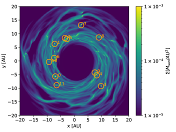
Figure 1: Surface density plot of the disk towards the end of the considered time frame ($t=156\text{yr}$). The clumps are marked in orange circles. The flocculent appearance of the disk can be seen as observed in Deng et al. (2020).

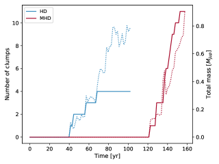
Figure 2: Evolution of the clump formation: Number of clumps (solid, left) and total mass contained in the clumps (dashed, right). Many more clumps form in the MHD case.

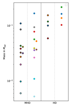
Figure 3: Masses of the resulting clumps in the MHD and the HD case. The dots with the black edge colour represent their masses at the time of fragmentation while the others show the mass averaged over the lifetime. In the MHD case, much smaller clumps can emerge, going below $10^{-2}M_{\text{jup}}$, this is already true at the time of fragmentation, when the clumps emerge.

In this section we describe the procedure to find the clumps in the snapshots, and to analyze them.

Towards the end of the simulation, at the last snapshot that we are considering, we identify clumps as follows; first, we find density peaks by selecting all particles above a certain density threshold and assign them to a cell on a grid that is superimposed on the particle distribution. The cells that contain such particles are marked as dense cells. We identify connected dense cells (clusters) on the grid and define all particles (including those below the density threshold) that lie in the corresponding cells as belonging to that cluster. Each of these clusters serves as the approximate location of a clump. For the density threshold we chose a value of $10^{-8}\text{g}/\text{cm}^{3}$ which amounts to $\approx 100$ times the average density in the simulation in the clump-forming radial extent of the disk. The exact choice of this value does not make much of a difference since the exact extension of the clumps are determined in the next step by identifying their gravitational boundedness.

In the next step, we start by determining the exact location (particle-wise) of a density peak within the cluster which we use as a guess for the corresponding clump’s centre. Around this point we introduce concentric shells (radial bins). Starting from the centre, we increase the radius by gradually determining if a certain shell is bound to the clump that is defined using all particles inside the corresponding radius of the shell. The gravitational boundedness is determined by calculating for each particle the potential energy with respect to the clump, the kinetic and the internal energy. The radius of the clump is finally defined using the inner end of the first unbound shell encountered.

Since we are interested in the clump’s evolution and their origins, we now trace them back to earlier snapshots. This is done by determining all particles that are within the clump’s radius and then identifying the same particles at earlier snapshots. Now there are two ways to proceed.

First, considering only this subset of particles, we find the position of their density maximum, i.e. where they congregate the closest. This position is then taken as the clump’s centre at the earlier snapshot. The radius of the gravitationally bound region is then determined in order to identify the clump. We measure quantities such as their mass, angular momentum and energy. The method just described, however cannot be used indefinitely backward in time since there is no well defined density maximum in the very early stage of clump formation, before a bound clump is present. It can only be extended back to the time when the clump first becomes bound (and somewhat before that). We check that our clump is still well-defined by evaluating the fraction of particles originally found in the clumps identified at a later stage but not included in the overdense region. At the time when the clump is bound, this fraction is low ($\lesssim 20\%$), meaning that there is no big change in the particle membership of the clumps after they become bound, namely their initial stage reflects the ”in-situ” flow.

Additionally, we are also interested in the regions of the disk at earlier times where the clumps will emerge in order to calculate disk properties relevant for their formation such as the Toomre or Jeans mass. For the latter we use a second method; we identify the clump-forming regions by finding the ensemble of particles that will be later incorporated in the clumps.

Fig. 1 shows a density plot of the simulation towards a time when all the clumps that become gravitationally bound have formed. The small scale structure that was observed in Deng et al. (2021) can also be recognized in this plot. The evolution of the clump population is presented in fig. 2 showing the number of clumps and their total mass over time and also comparing to the HD-case. The clumps are counted as soon as they are determined as bound using the method described above. One can see that in the HD-case, there are much fewer clumps than in the MHD-case.

In Fig. 3, the masses of the clumps are shown. They are calculated by determining the bound radius as described above and then summing up the mass of all the particles inside. The plot then shows their average mass from the time they become bound. Further, also the masses at the time when they first become bound are shown. As can be seen in the plot, in the MHD case, the clumps’ masses are generally lower and can have a much greater variation than in the HD case. Indeed, in the magnetized disks there are many low-mass clumps going below the mass of Neptune (Deng et al., 2021). We also note that the difference between the MHD and the HD case is already present at the onset of fragmentation.

In summary, the difference between the clumps in the MHD case and the HD case is two-fold; first, the clumps evolve differently when they are embedded in a magnetized disk (e.g. they have lower growth, and are protected from tidal disruption, see Deng et al. (2021)). Second, the initial fragmentation stage is different as the MHD clumps have smaller masses from the beginning and fragmentation is more plentiful.

3 Numerical Results

3.1 Predicted mass scales

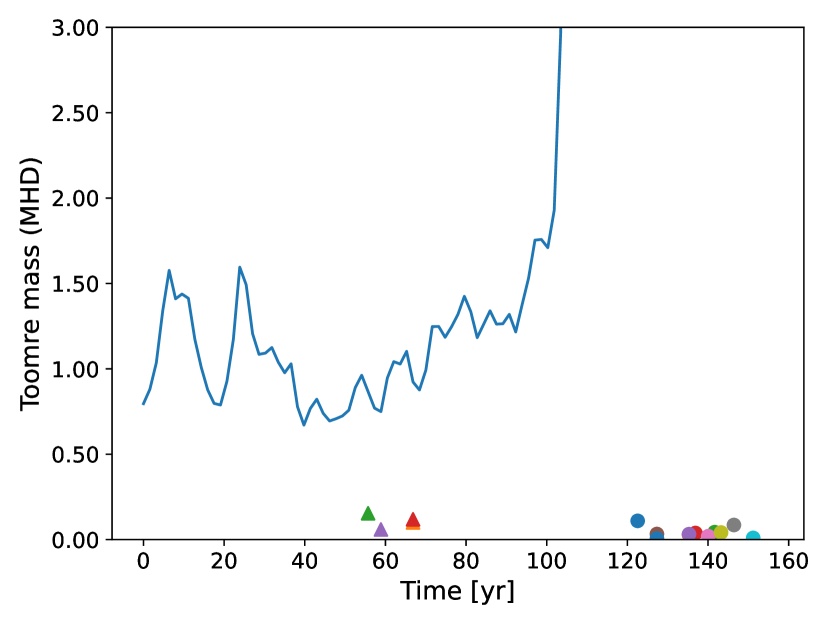
(a) Toomre mass over time. Generally, the masses of the clumps are greatly overestimated.

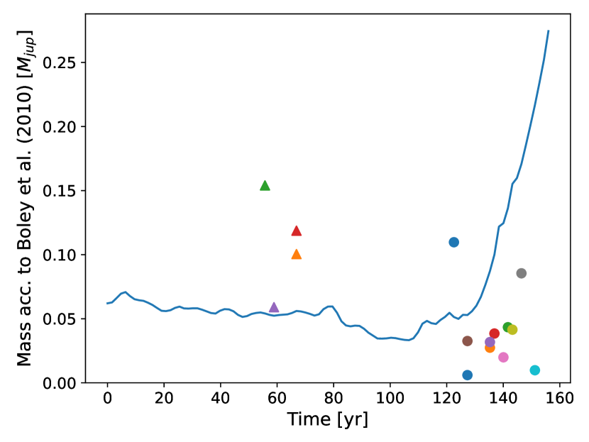
(b) Predicted mass according to Boley et al. (2010) using the same procedure. This theoretical prediction provides a better estimation than the Toomre mass (fig. 4) but does not explain the difference between the MHD and the HD case.

Figure 4: Toomre mass and mass prediction according to (Boley et al., 2010) determined using the backtraced regions of particles. At each snapshot in time, the particles that will later form the clump are identified and the quantities are measured. Then we average over the different clumps so the resulting values in the early stages are an average prediction for the clump masses (see second method described in section 2.2). At fragmentation, the Toomre mass and later also the Boley mass greatly increase since the background assumptions of the theories become invalid. Shortly later, the clumps become bound and are marked with a corresponding dot. As a comparison, the clumps arising in the HD simulation are shown with a triangle.

From Toomre’s theory of disk instability one can derive an estimate for the mass of the clumps by assuming that the collapsing region has a characteristic size of order the Toomre-most-unstable wave length $\lambda_{T}$: $M_{\text{Toomre}}=\pi\left(\frac{\lambda_{T}}{2}\right)^{2}\Sigma$. This estimate is shown in fig. 4 where we identified the fragmenting regions in the early snapshots of the MHD simulation (using the second method described in section 2.2) and determined a representative Toomre mass at any given time by averaging over the Toomre mass values obtained from the back-traced particles of the different clumps. Only the early snapshots in fig. 4 should be taken into account since the Toomre theory assumes an equilibrated disk which is better fulfilled before it fragments – when the clumps collapse the measure becomes invalid.

It can be seen that the predicted mass is around $1M_{\text{jup}}$. The masses observed in the MHD simulation reach down to $0.006M_{\text{jup}}$ – (see fig. 3) all being much lower than the prediction. Although higher, the masses of the clumps in the HD simulation are still below what would be expected from the Toomre mass. This means that additional effects have to be considered to study the nature of the collapse – both related and unrelated to the magnetic field. These effects could be the vertical extension of the disk, turbulence which could be induced or altered through the magnetic field or a direct effect of the magnetic field on fragmentation. We investigate the latter effect in section 4.

While Toomre’s theory assumes a thin background axisymmetric disk with differential rotation, the minimum collapsing mass should be comparable to the Jeans mass since that neglects rotation which affects the longer wavelength branch in Toomre instability theory. One can thus calculate the Jeans mass of the backtraced regions; also, this simplistic estimate is definitely too high for explaining the observed clumps masses.

A different model to estimate clump masses has been presented in Boley et al. (2010), which attempts to capture the actual dynamics in a non-axisymmetric disk. The model was verified against 3D radiative simulations of protoplanetary disks, and more recently was also shown to match well the results of fragmentation in high redshift galactic disks (Tamburello et al. 2015). Fragmentation, as seen from numerical simulations, does indeed occur in spiral arms rather than directly from the axisymmetric background flow (Mayer et al. 2004; Durisen et al. 2007). Instead of a homogeneous, axially symmetric background flow, the initial state is a spiral density wave identified as an overdensity whose strength is proportional to the local Mach number of the flow, which leads to velocity gradients that determine the region that can collapse. Considering also finite thickness, namely that the spiral arm has a vertical extent of order the disk scale height, they obtain the following mass estimate:

$$M_{f}=4\frac{c_{s}^{3}}{G\Omega f_{g}}$$ (7)

with $c_{s}$ the sound speed, $\Omega$ the angular frequency and $f_{g}$ a form factor to account for effects from self-gravity. (Boley et al., 2010) estimated $f_{g}\approx 1.8Q$. This is compatible with the considerations in Deng & Ogilvie (2022) where they suggested a solitary ring structure as a transitory state in which spiral density waves would emerge, and then collapse would eventually ensue in the flow entrained by them. Measuring $Q$ in our simulations by tracing back the clump’s particles in time leads to values of $Q\approx 1.15$ in the early phases of the simulation. We present the resulting estimate in fig. 4. The resulting mass lies around $0.05M_{\text{jup}}$, a bit higher at the beginning of the simulation. While this estimate lies indeed much closer to the resulting clump masses, any eventual effect of the magnetic field is not taken into account. The lower-end of the clump masses is still well below the estimated value. Also, when tracing back the particles of each clump individually and determining the estimated mass separately, namely without averaging, the mass estimates do differ significantly from the initial masses of the fragments.

3.2 Energetics of clump-forming sites before the collapse

As we seek the reason for the higher fragmentation rate and the lower mass fragments in the MHD case one should explore how the magnetic field itself can influence the fragmentation process. It could either directly change the physics during the collapse or indirectly, for example by stirring turbulence. Indeed, in their study of the mean flow properties of self-gravitating disks with and without magnetic fields, Deng et al. (2020) showed that magnetized disks are more turbulent relative to unmagnetized disks because Maxwell and gravitational stresses concur to generate a larger overall stress, resulting in enhanced angular momentum transport. In either case, the magnetic field is expected to affect the dynamics of the material because at a minimum an additional force, namely the Lorenz force, enters the equations of motion of fluid elements. Therefore it is important to know the relative contribution of the magnetic field, and of turbulence, to the energetics of those regions of the disk, along spiral arms, that will turn into clumps.

In fig. 5(a) the relation between the magnetic and the turbulent kinetic energy is shown for the individual clumps. The specific magnetic energy density is calculated via $E_{B}=\frac{B^{2}}{4\pi\rho}$ where $B$ is the magnetic field and $\rho$ the density. To quantify the turbulent kinetic energy, we first defined the velocity dispersion of a particle. We used kernel-smoothing to calculate a mean velocity around a particle $i$ using a number of neighbours of $n_{\text{smooth}}=32$, $\langle v_{i}\rangle=\sum_{j}v_{j}W\left(\frac{x_{j}-x_{i}}{h}\right)\frac{m_{j}}{\rho_{j}h^{3}}$. Here $W$ denotes the smoothing kernel for which we used the cubic spline (Monaghan, 1992), $h$ the smoothing length, $x_{i}$, $m_{i}$, $\rho_{i}$ the position, mass and density of particle $i$. To arrive at the velocity dispersion we smoothed over the square deviation of the mean velocity $\langle v_{i}\rangle$:

$$\hbox{$\sigma_{i}=\sqrt{\sum_{j}\left(v_{j}-\langle v_{i}\rangle\right)^{2}W\left(\frac{x_{j}-x_{i}}{h}\right)\frac{m_{j}}{\rho_{j}h^{3}}}$}.$$ (8)

Then we calculated the turbulent kinetic energy via $E_{\text{turb},i}=\frac{1}{2}m_{i}\sigma_{i}^{2}$.

Similarly, in fig. 5(b) the relation between the magnetic and the internal energy is shown. The specific internal energy is available directly as a result of the simulation. In both plots, we concentrate on the clumps 15 snapshots (corresponding to $\approx 24\text{yr}$) of the simulation before they become bound since we are interested in the influence of the magnetic field as a precondition of the fragmentation process. The results are then shown together with the mass of the respective clumps.

To trace the particles back in time, we used the first method described in section 2.2 namely we followed the density maxima as the centres of the distribution of particles associated to a given clump backwards in time. Despite of the clumps not yet being bound at earlier time, this method still traces the clump-forming regions until a density maximum can be defined and identified (see section 2.2).

It can be seen that the magnetic energy is larger than the turbulent kinetic energy for all the clumps. For most of them the difference is around an order of magnitude. This means that the energy stored in the magnetic field is much greater than in the turbulent motion of particles. Therefore knowing the structure of the magnetic field is important to understand the gas motion.

However, when comparing with the internal energy of the gas, the magnetic field is significantly smaller. Therefore the thermal gas pressure is still the most important of the quantities considered so far. We anticipate that, except in the inner regions of the clumps, the total kinetic energy, including the non-turbulent component of the velocity field, is the dominant contribution counteracting gravitational potential energy, because clumps are rapidly rotating. This will be studied in section 3.4. In the interior of clumps, instead, internal energy is always the main component establishing equilibrium, as it will be further assessed in section 3.4. However, from Deng et al. (2020) we know that the presence of magnetic fields change the dynamics of the flow: first, the magnetic field ignites turbulence in the disk and second, the presence of a magnetic field leads to smaller-scale structures in the disk. The question remains if the differences in fragmentation in the MHD case is a direct consequence of the presence of the magnetic field during this process or if it is a secondary effect arising from different features of the environment. The result from fig. 5(a) would be compatible with the magnetic field directly impacting fragmentation since it carries much more energy in itself than the turbulent component of the kinetic energy. In section 4 we discuss a possible path of how the magnetic field could affect fragmentation.

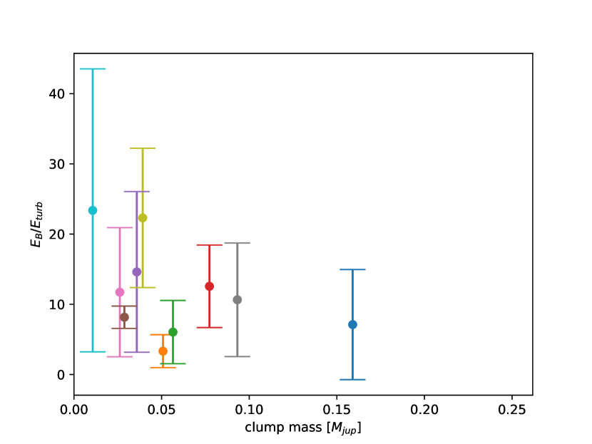
(a) Magnetic energy relative to turbulent energy

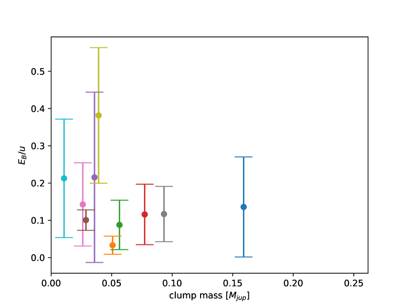
(b) Magnetic energy relative to internal energy ($\beta_{\text{plasma}}^{-1}$)

.

Figure 5: Magnetic energy relative to turbulent energy and relative to internal energy, averaged 15 snapshots (corresponding to $\approx 24\text{yr}$) before up until the existence of a bound structure. Each dot represents a clump, the bars show the standard deviation of observed values. The magnetic energy is roughly an order of magnitude greater than the turbulent kinetic energy compatible with a direct effect on fragmentation. The internal energy is larger than the magnetic energy for all clumps.

3.3 Energetics of the clumps after collapse; the role of the magnetic field

In this section we want to give an overview of the evolution of the clumps during their early stages right after they become bound and to investigate the role of the magnetic field during this time. For that, we focus on the magnetic, but also the turbulent kinetic energy and the internal energy of the gas. It was already mentioned in Deng et al. (2021) that the magnetic field is amplified in and around the clumps and may shield them from further growth but may also prevent their disruption because of its relative strength compared to the kinetic energy. We also look at this amplification effect more closely in this section.

We now follow the evolution of a typical clump in the MHD simulations. For that, we present two-dimensional cuts and radial profiles of the density, the magnetic field and the velocity field. We choose clump nr. 5 from fig. 1 as it belongs to the lower-mass end of the clumps distribution ($0.03M_{\text{jup}}$), our implicit assumption being that lower mass clumps should be most affected by the magnetic field as they are absent in the non-magnetized case (HD simulations). We start at a simulation time of 127 yr. At this time, some of the clumps are already bound while others are still forming. Clump 5 is just becoming bound. It is forming in a filament structure of increased density, along with three other clumps (0, 1 and 8). In our subsequent analysis we are interested in the configuration of the magnetic field and how it could affect the clump and its surroundings.

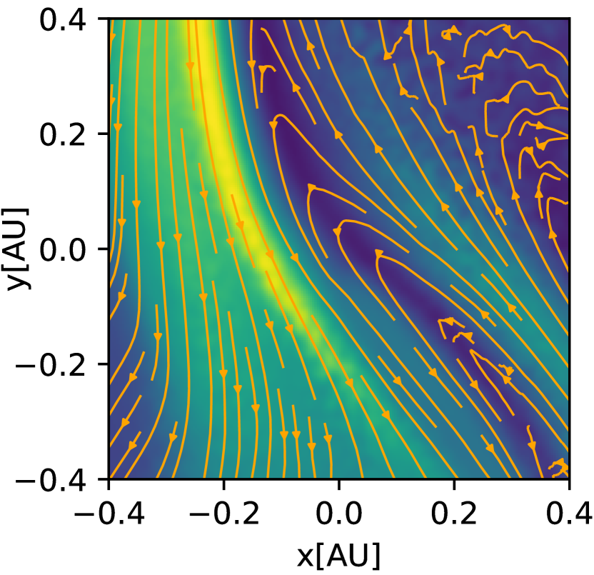
(a) horizontal cut with magnetic field lines, clump 5, 127 yr

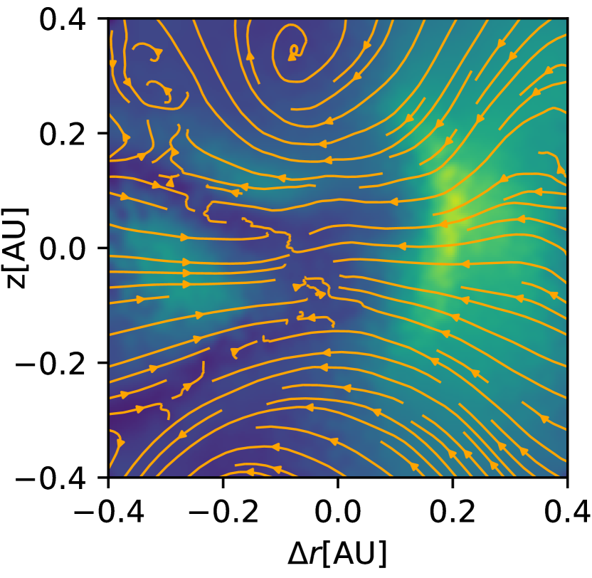
(b) vertical cut with magnetic field lines, clump 5, 127 yr

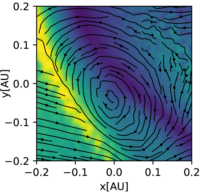
(c) horizontal cut with velocity field lines, clump 5, 127 yr

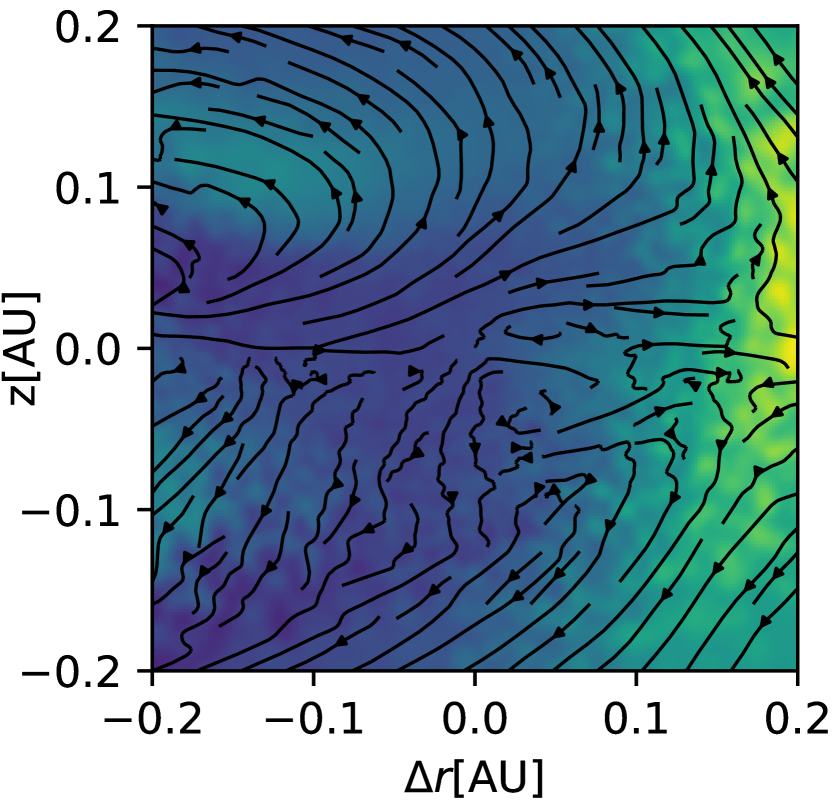
(d) vertical cut with velocity field lines, clump 5, 127 yr

Figure 6: Evolution of clump 5: First bounded stage. Top: magnetic field strength and magnetic field lines in a region of $0.4\text{AU}$ around the clump. The horizontal cut on the left is aligned with the disks plane while the vertical cut on the right shows the height $z$ over the disk’s radial coordinate $\Delta r$. Bottom: The same location but showing the velocity field lines (again magnetic field strength in the background) instead of the magnetic field lines in a region of $0.2\text{AU}$. On both sides of the high-density filament, the magnetic field is increased. When comparing the magnetic field energy to the internal energy, one arrives roughly at a value of $\beta_{\text{plasma}}^{-1}\approx 0.5$ for the outer regions in the plot.

Fig. 6 shows the configuration of clump 5 at this time. In the following two-dimensional profiles the clump is always centred using its density maximum. In the top of fig. 6 the magnetic field strength is shown around a region of $\pm 0.4\text{AU}$. The clump will have a radial extension of $\approx 0.1\text{AU}$ (see e.g. Fig. 7). The orange lines show the magnetic field lines. In the horizontal cut on the left which is made parallel to the disk, it can be seen that the centre of the clump lies in an elongated region of low magnetic field strength which is also of a higher density. To the side of this region the magnetic field increases. This effect of an increasing magnetic field along a thin elongated region of higher density can also be observed around other clumps.

Also, contrary to the other clumps, here the magnetic field reverts its direction when passing through the high-density filament. This can be explained by looking at the plots below which show a smaller extract with the same centre. Here, the velocity field (black lines) is drawn over the magnetic field strength: The flow of the collapsing region moves inwards from two opposite sides, thereby growing the high-density filament. During this process magnetized material is transported close to the filament, enriching the magnetic field there.

What magnetic field strength do we expect the filamentary structure to have? We assume that this structure emerged from a partial collapse in two directions orthogonal to the direction of the filament. Assuming also ideal MHD without resistivity, the flux through a surface defined via any particles remains constant over time. If we choose this surface to be orthogonal to the filament’s elongated direction, then the area of the surface scales as $A\propto\rho^{-1}$ over time (since we assume no collapse in the elongated direction). Since the conserved flux is defined as

$$\Phi=\int B\cdot dS$$ (9)

where the integral goes over the chosen surface, the magnetic field $B$ has to scale as $B\propto\rho$. The density at the boundary of the filament increases roughly four-fold. So the magnetic field can be expected to also be four times as strong along the filamentary structure. This is about what is observed in fig. 10, when assuming a background strength of the magnetic field of $\approx 0.8\text{Gs}$ (see also fig. 8).

While the magnetic field is increased at the boundary of the filament, the low magnetic field region in the middle probably arises because here the flow combines two regions of opposite magnetic fields directions. Further there is probably a higher gas pressure in this region because of the higher density. An effect of this can be seen at the bottom right of the figure where a vertical cut of the clump’s region is shown. In the vertical cut we show the height ($z$) and the change of the radial component $\Delta r$ measured from the central star. In this case, the prominent region of a strong magnetic field from the horizontal cut on the left is now in the right side of the figure at higher radii. It can be seen that the flow escapes from the central region of higher density ($z=0\text{AU}$) up- and downwards. In the vertical cut on the right vortices of the magnetic field can be seen above and below the clump. Such vortices are also observed around other clumps.

Already $13$ years later, the development of a magnetic shield can be observed which is shown in fig. 7. Again, horizontal cuts (left) and vertical cuts (right) are shown. The magnetic shielding effect was already discovered in Deng et al. (2021) where it was found that the clumps were surrounded by regions of high relative magnetic energy which control the flow around the clump and thus shield it from disruption but also slow its further growth. The top and bottom of fig. 7 show the situation at two consecutive snapshots, with $1.6$ years time difference in between (compared to an orbital period of $23$ years). At this stage, the clump already developed a significant rotation and is quite extended (see fig. 10 and section 3.4). The rotating flow drags the magnetic field around the clump thereby forming a shield of increased magnetic field strength. In the vertical cut on the bottom right it can also be seen that the flow coming from the left does a sharp turn upwards when entering the region of high-magnetic field strength. This could reflect a deflection from the magnetic field. In the later evolution, this magnetic field shield becomes weaker, possibly due to Ohmic dissipation. At later times it seems to regain strength.

In fig. 8 we show the magnetic field strength for the same clump as a radial profile at various times represented by the different curves. The radius $r$ measures the distance from the clump’s centre – the bound radius at each time is marked with a dot which is calculated as described in section 2.2: At a time of 131 yr, the clump is first bound. It can be seen that at a time of 143 yr, when we observed the magnetic shield, a strong increase of the magnetic field is measured. At $150$ yr, the magnetic field is again low but begins to increase at $156$ yr. Such an oscillating behaviour can also be seen for other clumps, however mostly the peak is inside the bound radius. What is the timescale for the Ohmic dissipation? Starting from eq. 5 and assuming zero velocity $v=0$, one can estimate the time scale as:

$$\frac{\Delta B}{\Delta t_{\text{diss}}}\approx\nu\frac{\Delta B}{\Delta r^{2}}\implies\Delta t_{\text{diss}}\approx\frac{\Delta r^{2}R_{m}\Omega}{c_{s}^{2}}$$ (10)

where we substituted $\eta=c_{s}H/R_{m}$ with $H$ the scale height and $c_{s}$ the sound speed and used that $H\approx c_{s}/\Omega$. $\Omega$ is the rotational frequency around the central star. In this equation we take for $\Delta r$ the radial size of the magnetic shield. When plugging in values that arise at the boundary of the filament one arrives at a dissipation time of roughly $t_{B}\approx 5yr/2\pi$ which means that changes in the magnetic field should be expected between the snapshots which are taken every $10yr/2\pi$.

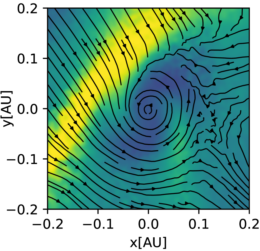
(a) horizontal cut with velocity field lines, clump 5 at 141 years

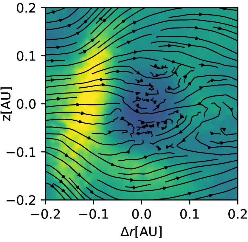
(b) vertical cut with velocity field lines, clump 5 at 141 years

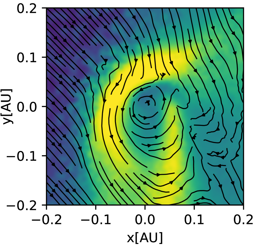
(c) horizontal cut with velocity field lines, clump 5 at 143 years

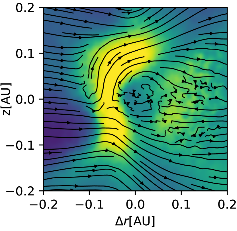
(d) vertical cut with velocity field lines, clump 5 at 143 years

Figure 7: Evolution of clump 5: Build-up of a magnetic shield. The plots on the left are horizontal cuts in the disk’s plane, the plots on the right are vertical plotting the height $z$ and and the radial coordinate w.r.t. to the central star. They show the magnetic field strength with the velocity field lines at two consecutive snapshots (top: $142$ yr, bottom: $143$ yr).

We now compare the magnetic energy to other quantities to determine its importance. First, it is compared to the turbulent kinetic energy. The turbulent kinetic energy and the magnetic energy are measured as described in section 3.2.

The middle row of fig. 9 shows radial profiles of the magnetic energy relative to the turbulent kinetic energy: Again, the different curves show the situation at different stages in the clump’s evolution. We show the profiles up to a distance of $1\text{AU}$ since we are interested in the region close but clearly outside the clump. This value corresponds to a distance a bit larger than twice as much as the maximum bound radius of a clump that we observe in the simulations.

It can be seen that generally the magnetic energy is more important than the turbulent kinetic energy since it is of a larger magnitude. This is especially true for the later stages after the clump has become bound. The great increase at $137$ yr of clump 5 is because the clump is in an environment of low density and temperature. Often an increase in the relation between the magnetic field and the turbulent kinetic energy can be observed after the clumps have become bound. For example, in the middle-right plot of fig. 9, which shows the same relation for clump 8, it is even more clear that after the clump becomes bound, the magnetic field becomes significantly more important in its surrounding.

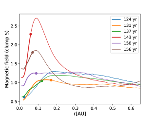
Figure 8: Radial profile of the magnetic field strength (in Gs) for clump 5 at various times. The bound radius of the clump at each time is shown with a dot. At 143 yr, shortly after the clump became bound, a peak of the magnetic field develops in the region of the bound radius. Later, the magnetic field decays but begins to increase again at 156 yr.

It is also interesting to compare the magnetic energy to the internal energy which is responsible for the gas pressure forces. This relation is shown in the top-center plot of fig. 9 for clump 5 and in the top-right plot for clump 8. Here, it is also visible that the magnetic energy is important compared to the internal energy. Again, this is more pronounced for clump 8 than for clump 5 where there is a single spike of the relation at 137 yr. The decrease in energy around $r=0.7\text{AU}$ at $156$ yr for clump 5 arises because of another clump forming nearby.

Both relations, internal energy density to magnetic energy density and turbulent kinetic energy density to magnetic energy density tend to become smaller at small radii inside the clump’s bound radius. This is because of the greatly increased density at these regions. Because of that, the same temperature yields a much higher internal energy density. Vice versa, the turbulent kinetic energy density is also increased at this region. In the next section we characterize the influence of various physical quantities on the evolution of the clump and show their relative importance at different locations in the clump.

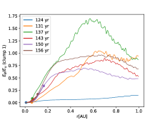
(a) $E_{B}/E_{u}$ of clump 1

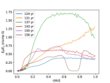
(b) $E_{B}/E_{u}$ of clump 5

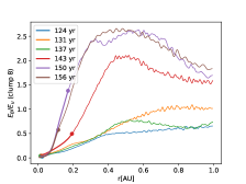
(c) $E_{B}/E_{u}$ of clump 8

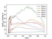
(d) $E_{B}/E_{\text{turb}}$ of clump 1

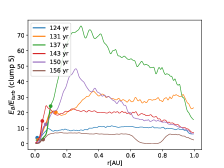
(e) $E_{B}/E_{\text{turb}}$ of clump 5

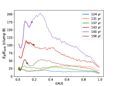
(f) $E_{B}/E_{\text{turb}}$ of clump 8

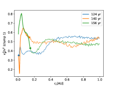
(g) $v_{\varphi}^{2}/v^{2}$ of clump 1

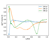
(h) $v_{\varphi}^{2}/v^{2}$ of clump 5

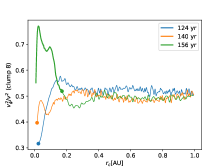
(i) $v_{\varphi}^{2}/v^{2}$ of clump 8

Figure 9: Top: Magnetic energy density relative to internal energy density ($\beta_{\text{plasma}}^{-1}$). In the vicinity of the clumps, the magnetic energy remains important when comparing to the internal energy. Middle: Magnetic energy density relative to turbulent kinetic energy density. The magnetic energy is generally of a larger magnitude than the turbulent kinetic energy, especially at the later stages of the clump’s evolution. Often, this relation increases after the clumps have become bound. Bottom: Relative rotational energy $v_{\phi}^{2}/v^{2}$. The plots show radial profiles of the mentioned quantities at different times and for three different clumps. Inside the bound radius, the motion is mostly rotation-dominated.

3.4 Rotation and clump dynamics

Until here, we focused on the properties of the flow in the very vicinity of the ensuing clumps. Their evolutionary path depends also on their internal properties which are investigated in this section.

Rotation has often been reported as dynamically important in clumps formed via disk instability (Mayer et al., 2004; Galvagni et al., 2011; Shabram et al., 2011; Helled et al., 2014) Therefore, we investigate its relevance in magnetized clumps as well. Additionally, the strength of rotation will also have implications on the rotation rate of an eventual planet resulting from further collapse. Fig. 10 shows again the configuration of clump 5 at two different times: On top at 140 yr, 8 snapshots after the clump became bound and at the bottom at 158 yr at the end of the analyzed simulations. The plots show the density with the velocity vector field for horizontal cuts aligned with the disk’s plane (left) and for vertical cuts perpendicular to the disk (right).

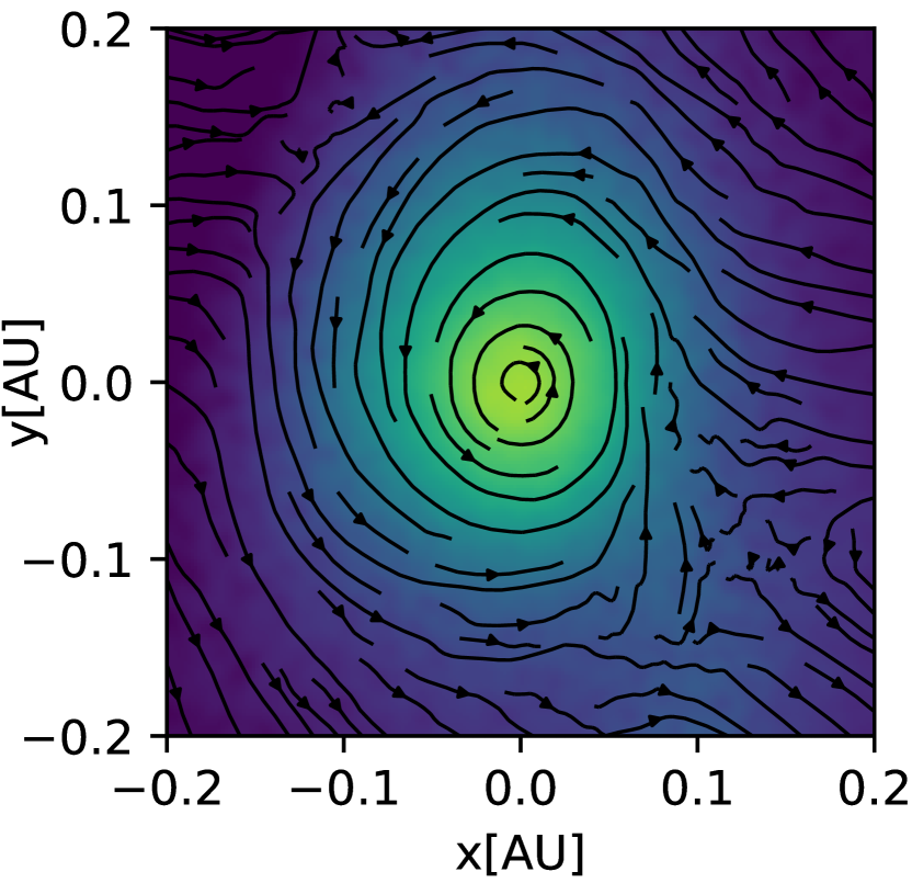
(a) horizontal cut with velocity field lines, clump 5, 141 yr

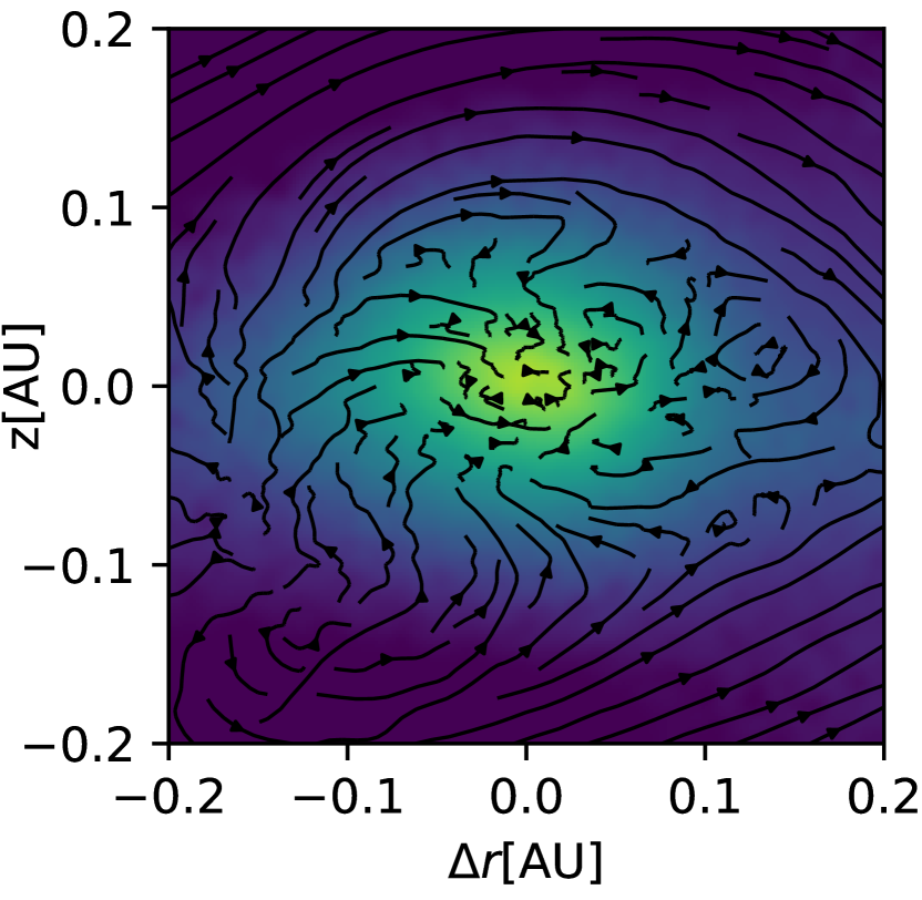
(b) vertical cut with velocity field lines, clump 5, 141 yr

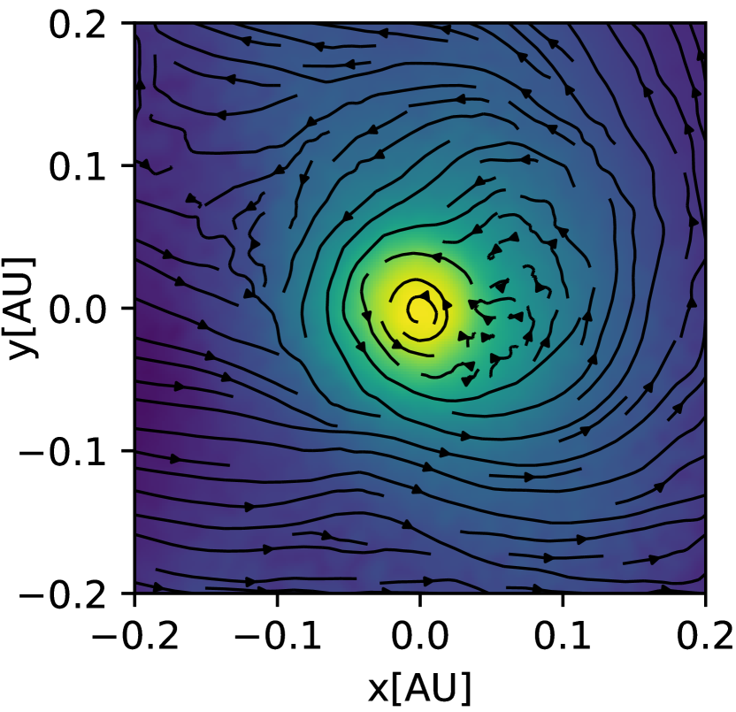
(c) horizontal cut with velocity field lines, clump 5, 158 yr

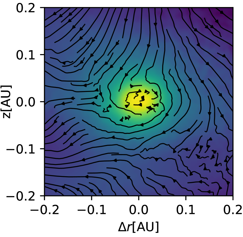
(d) vertical cut with velocity field lines, clump 5, 158 yr

Figure 10: Evolution of clump 5: Density at early (top) and later (bottom) stage (colour) and velocity field (black arrows). The horizontal cuts on the left are aligned with the disk’s plane and show a contraction of the clump over time. The vertical cuts on the right show that the clump is first elongated along the disk’s plane, whereas later it is more round.

It can be seen at the top left, that the clump at this earlier time has a wide-spread, almost elliptical region where rotation around the clump’s centre dominates the velocity field. At this stage the clump is probably sustained with rotation by the differential rotation of the surrounding gas of the disk.

In the vertical cut on the top right it can be seen that the clump at this stage has an almond-like shape that is elongated along the mid-plane. The surrounding material flows around this structure from smaller to larger disk’s radii. In the interior the flow seems to be erratic without showing a preferred pattern. The elongated shape could be a hint for the rotation to be important for stabilization at this stage since it only exerts a force in the rotating plane.

When looking at the later stages at the bottom, one sees that the shape of the clump has changed. From the horizontal cut at the bottom left it is visible that the clump has become denser than before and also seems to be concentrated in a smaller region. The velocity field only shows a clear rotating behaviour in the inner parts with radii $<0.05\text{AU}$. Further outside the velocity field still suggests some rotation although the flow seems to be in a more undetermined state.

The vertical cut at the bottom left shows that the clump has become much rounder than before and is no longer embedded in this almond-shaped high-density region. The flow at this stage mostly comes from the upper and lower end to the centre.

Now the clump’s rotation should be determined quantitatively. As in section 3.3 we show one-dimensional radial profiles of the clump. Here it seems more appropriate to use a cylindrical coordinate system since rotation is defined along an axis. We start by determining the main rotation axis of the clump. For that, we consider all particles inside the bound radius and determine their total angular momentum relative to the center of mass. The normalized angular momentum vector gives us the z-component of a cylindrical coordinate system. This vector points in the same direction as the orientation of the protoplanetary disk.

In that coordinate system we determine the azimuthal velocity $v_{\phi}$ of the particles. We then consider the squared relation to the total velocity $v_{\phi}^{2}/v^{2}$ thereby comparing the rotational to the total kinetic energy. Thus we can determine more quantitatively if the clump exhibits rotating behaviour. A radial profile of this relation is shown in the middle-bottom plot of fig. 9 for clump 5. A value of $1$ means that all kinetic energy is purely in rotation, if the energy is equipartitioned we would expect a value of $1/3$.

At the time of the blue curve, before the cuts of fig. 10 the curve is flat over a large region and sharpy decreasing in the interior. This decrease seems to come from vertical infall of material to the centre. At this stage, the clump is not yet bound.

At a later stage at $140$ yr (yellow curve) which represents the time of the top plots in fig. 10 the curve begins to increase when approaching the centre. Here, the clump is bound up until a radius of $\approx 0.15\text{AU}$. While at radii further out than $\gtrsim 0.2\text{AU}$ the curve is flat, inside it reaches values of $\approx 0.9$. Inside the bound radius, the clump exhibits strong rotation. At the even later stage at $156$ yr (green curve) which corresponds to the time of the bottom plots in fig. 10 the spike is even narrower and higher. Consistently, the bound radius is also smaller, somewhat below $0.1\text{AU}$, up to where the rotation is no longer dominating. This seems to indicate that the clump shrunk in radius during this time. This also confirms our method of measuring the bound radius as described in section 2.2. In all observed clumps we measure the behaviour of increased rotation near the centre after they are bound. Often however, the bound radius is more extended than what one would expect from simply estimating where the rotation curve becomes flat. On the other hand, if in an inner region the rotation is significantly enhanced compared to outside, the clumps seem to always be bound at least in that part.

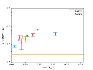
(a) MHD

(b) HD

Figure 11: Specific angular momenta of the clumps arising in the MHD and the HD simulation. They are significantly lower in the MHD case– probably because of the dissipation of the magnetic field. As such, they are closer to those of Jupiter and Saturn which are also shown for comparison.

From rotation we can also determine the total specific angular momentum $L/m$. This is plotted for each clump in fig. 11. It is calculated over the lifetime of each clump respectively where the dot indicates the mean and the bars are the standard deviation of the range of observed values. For comparison, the HD case is also plotted below. It can be seen that the specific angular momentum measured in the MHD case is significantly smaller than in the HD case. Here, it should be noted that it has already been found in Mayer et al. (2004) that the angular momentum of protoplanetary clumps observed in simulations of fragmenting disks is an order of magnitude too high when comparing with those of the gas giants in our solar system. The specific angular momenta of the gas giants (Helled et al., 2011) are also shown in the plots – the protoplanets in the MHD case are much closer to them than they are in the HD case. The reason for this difference could be the resistivity. If the magnetic fields are enhanced by the clump’s rotation the resistivity could remove the magnetic energy over time, preventing a possible saturation of the magnetic field and thereby leading to a continuous depletion of rotational energy. This would eventually bring the specific angular momentum more closely to that of Jupiter.

An important effect of rotation could be the stabilization of the clump against collapse because of the gravitational force. Another stabilizing force inside the clump is the gas pressure. Fig. 12(b) shows the evolution of 1d profiles of the specific internal energy. This quantity is directly proportional to the gas temperature and thus also determines the gas pressure. It can be seen that before the bound stage (blue curve), the internal energy profile is flat meaning that the center of the clump forming region has the same temperature as its surroundings. At $140$ yr, corresponding to the top plots in fig. 10 the internal energy is slightly enhanced in the region inside the bound radius. However this enhancement is only weak indicating the early stage in the clump’s evolution where it has not reached its final density. At this stage, the relatively cold temperature could mean that rotation is more important leading to the elongated shape of clump 5 at this time which was described before. At later times, at $156$ yr (green curve), the internal energy clearly increases in the centre indicating the evolved state of the clump.

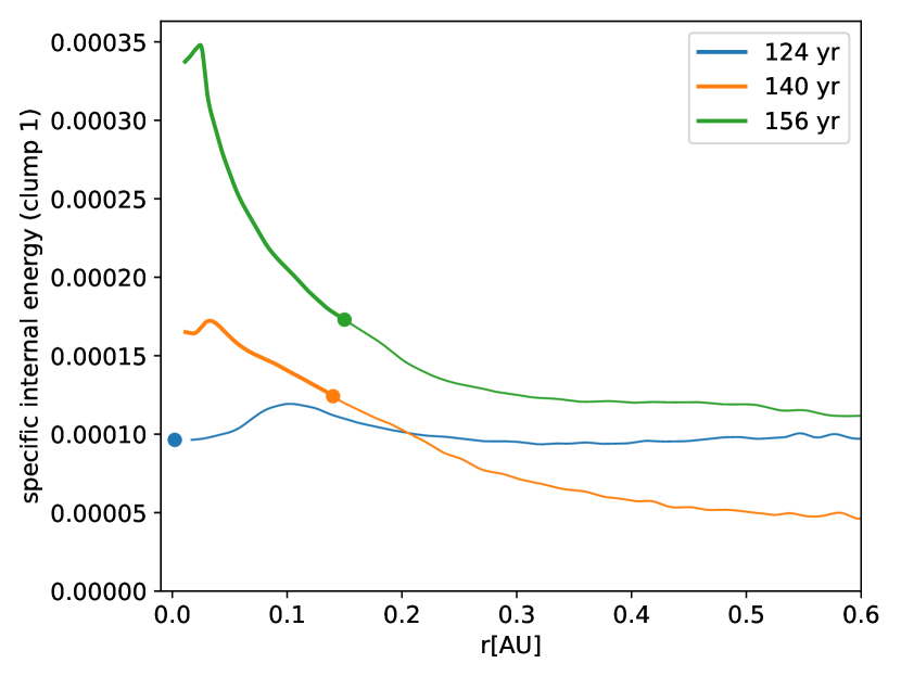
(a) clump 1

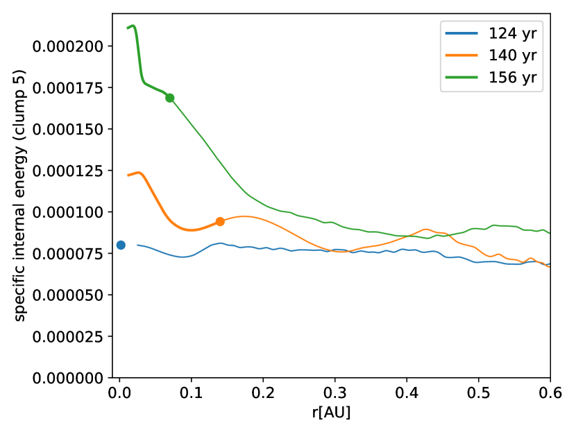
(b) clump 5

Figure 12: Radial profiles of the specific internal energy of clump 1 and 5. After the clumps are bound, they heat up in the centre. The gas pressure, which is determined through the specific internal energy, is important for stabilizing the clumps.

Since it was already shown in section 3.3 that there are significant magnetic fields present inside the clumps it remains to characterize them and discuss their effects inside the clump. The magnetic fields could act in both ways on the clump, stabilizing or compressing.

We estimate their importance relative to the other forces (gravity, gas pressure and rotation) by resorting to a one-dimensional model of the clump. For that, we calculate radial profiles of the quantities thereby ignoring angular features.

The force on a volume element $\delta A\delta x$ consists of several force terms:

$$\delta F=(g\rho\delta x+\Delta P_{g}+\Delta P_{B}+\cos(\theta)\rho \delta xv_{\varphi}^{2}/r_{c})\delta A$$ (11)

The gravitational acceleration is

$$g=G\frac{M_{\text{encl}}}{r^{2}}$$ (12)

with $M_{\text{encl}}$ the enclosed mass in a sphere of radius $r$. The pressure difference between two sides of the volume element is defined via the internal energy:

$$\Delta P_{g}=(\gamma-1)\rho\Delta u$$ (13)

The magnetic pressure term is derived from the magnetic energy density

$$\Delta P_{g}=\frac{\Delta(B^{2})}{8\pi}.$$ (14)

In equation 11 we also subtract a centrifugal force term representing the stabilizing effect of rotation. The rotation is assumed to happen around a rotation axis. We define this force in terms of the cylindrical radius $r_{c}$ (the distance to the rotation axis), the angular part of the velocity (defined in the cylindrical coordinate system) $v_{\phi}$ and the angle $\theta$ for the angle between the spherical radial direction and the cylindrical radial direction.

Fig. 13(a) shows the contribution of the various forces at $142$ yr of clump 5. It can be seen that inside the clump’s radius the dominating stabilizing force is the gas pressure, being larger than the rotational force. This is despite the clump showing significant flatness (see Fig. 10 top right). Inside this clump, the magnetic field exerts a compressing force. Somewhat outside the clump’s radius the magnetic field becomes stronger and its pressure force points outward being of a similar order as the gas pressure and the rotational force. Fig. 13(b) shows the same for clump 8 at $151$ yr. There, it can again be seen that the gas pressure dominates over the other stabilizing forces inside the clump. This is observed in all of the clumps from which we can make the conclusion that the clumps at this stage are pressure-supported instead of rotation-supported. For clump 8, it can also be seen that the magnetic field is even stronger than the other stabilizing forces in a region outside the bound radius. That the magnetic field has the highest contribution compared to the other forces around and somewhat outside the bound radius is a general feature we observe in the clumps.

The resulting radial acceleration from these force contributions shows a characteristic difference between taking the magnetic field into account and neglecting it. As expected, the magnetic field has the greatest effect around the bound radius. Somewhat outside the bound radius there is for most clumps a region where the radial acceleration is higher meaning that material is prevented from accreting on the clump. At the bound radius the situation is sometimes reversed (e.g. clump 5) and the magnetic field acts compressing. Further inside and far outside the effect is small. This behaviour can be explained by looking at fig. 8. At this time, the magnetic field has a sharp peak just outside the bound radius of the clump. Therefore the magnetic pressure force points inwards when going closer to the centre and outwards when going in the other direction. The first effect can be seen for most of the clumps: When including the magnetic field, the force balance is shifted to the outward direction outside the bound radius.

For clump 8 this effect is even more pronounced. While here, in the situation without the magnetic field, the system would be collapsing up until a radius of $\approx 0.5\text{AU}$, if the magnetic field is included, only a region of $\approx 0.3\text{AU}$ has a clear negative force. The other effect of a compressing force at the bound radius can however not be observed for the other clumps possibly because for them the magnetic field is dominated by the other forces at this radius.

This observation of an outward pointing force arising from the magnetic field is consistent with the findings in Deng et al. (2021). There the simulations were continued without the magnetic field after the clump formation and it was found that the further evolution of the clumps changed compared to simulations that continued to include the magnetic field. Namely, the clumps were disrupted if no magnetic field was present due to the missing of the shielding effect.

The analysis presented in this section was carried out at a time when the clumps have already formed and are gravitationally bound. It remains however to find reasons for the smaller initial clump mass at the very onset of fragmentation in the MHD simulations compared to the HD ones. This will be the focus of the next section.

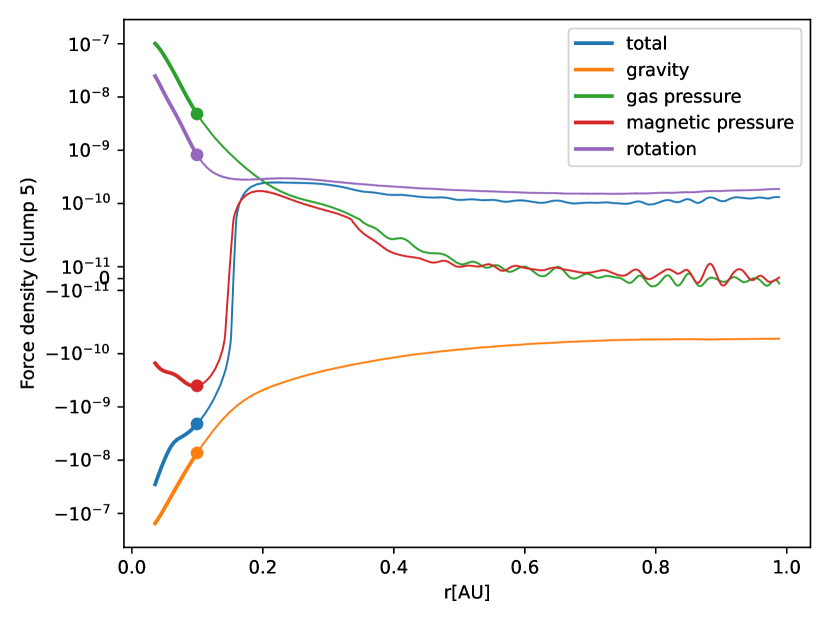
(a) Clump 5

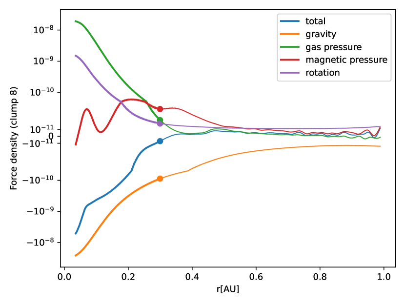
(b) Clump 8

Figure 13: Resulting force density $\delta F/\delta A\delta x$ for two different clumps. Top: Clump 5. Inside the bound radius (marked with a dot), the gas pressure is the dominating stabilizing force although rotation also plays a role which could explain the observed flatness in fig. 10. The magnetic field acts compressing up to a certain radius until it pushes matter outwards corresponding to the magnetic shield visible in fig. 7. Bottom: Clump 8. While at small radii inside the clump, gas pressure and rotation dominate over the magnetic field (possibly due to the higher density), the magnetic field becomes more important further out, around the clump’s bound radius (marked with a dot).

4 A physical description of gravitational instability in magnetized disks

4.1 A linear perturbation theory approach

Here we will try to address how different the initial development of clumps is in a magnetized flow as opposed to an unmagnetized one. This is important since, as we reported, the masses of clumps in magnetized disks are significantly lower than those in unmagnetized ones since the beginning (since they become bound), which suggests the effect of magnetic pressure in stifling gas accretion, suggested in (Deng et al., 2021), can not be the only reason behind the low masses of clumps (see fig. 3).

To this aim, we investigate how the presence of the magnetic field could change the fragmentation. Let us now turn back to Elmegreen’s analysis on fragmentation in magnetized galactic disks (Elmegreen, 1987). Starting with the magneto-hydrodynamical equations he assumed first-order perturbations. Then the equations were evolved numerically and the response of the system to a perturbation was studied. We note that the results presented in this paper include resistivity. However, similar results have been observed for ideal MHD simulations (Deng et al., 2020) where we expect even more prominent differences since the magnetic field is not restrained. For simplicity, we consider ideal MHD in this section. The ideal magneto-hydrodynamical equations describe the gas motion by considering gas pressure, self-gravity and magnetic fields:

$$\frac{\partial\rho}{\partial t}+\nabla(\rho v)=0$$ (15)

$$\frac{\partial\vec{v}}{\partial t}+\vec{v}\cdot\operatorname{grad}\vec{v}=-\frac{1}{\rho}c_{s}^{2}\operatorname{grad}\rho-\operatorname{grad}\Phi\ +\frac{1}{\mu_{0}\rho}(\vec{\nabla}\times\vec{B})\times\vec{B}$$ (16)

$$\Delta\Phi=4\pi G\rho$$ (17)

$$\frac{\partial B}{\partial t}=v\times(v\times B)$$ (18)

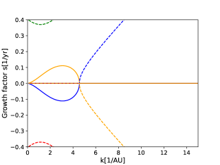
(a) Solutions of dispersion relation at t = 0

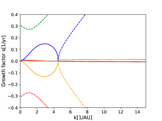
(b) Solutions of dispersion relation at t = 0.5 / $\Omega$

Figure 14: Solutions of the dispersion relation for shearing perturbations at different times (different values of $k_{x}$), plotted over the wavenumber. The imaginary parts of the solution are solid and the real parts are dashed. If there exists a solution with a non-zero imaginary part, perturbations can grow in the corresponding regime. At large wavenumbers, there exists only a real (oscillating) solution.

In a localized cartesian coordinate system in the disk where the x points in the radial and y in the transversal direction, the local background flow can be approximated as

$$\begin{pmatrix}v_{x}\\ v_{y}\end{pmatrix}\ \simeq\ \begin{pmatrix}-\Omega(r_{0})y\\ 2\mathcal{A}x+\Omega(r_{0})x\end{pmatrix}$$ (19)

with $\mathcal{A}$ being one of the Oort’s constant (Binney & Tremaine, 2008) that represents the shear arising from differential rotation. By defining a dimensionless shear-parameter $\alpha\coloneqq\mathcal{A}/\Omega$ the shear of the flow can be more conveniently quantified which makes it radius-independent if the angular velocity follows a power law in terms of the radius (e.g. in a Keplerian orbit).

Elmegreen considered linear perturbations to an equilibrium solution that are proportional to $\exp(ik_{y}(y-2\mathcal{A}xt))$ which means they start azimuthally oriented and are then sheared out over time. He then integrated the perturbative solution numerically over time for various parameters of the magnetic field and the shear rate. Elmegreen found that the effect of the magnetic field depended hugely on the value of the shear parameter. In a strong shear case which corresponds to $\alpha=-0.5$ as for a flat rotation curve of a galactic disk, the magnetic field stabilized the disk. Here, an increase in the magnetic field resulted in a stronger damping of the perturbations similar to what was found in the last section. On the other hand in a weak-shear case which corresponds to $\alpha=-0.05$ the result however was very different. Here, it was found that the magnetic field severely destabilized the disk. While the response of the system to the perturbation was stable without a magnetic field, even a small value of the magnetic field led to a huge amplification of the perturbation. The stronger the magnetic field, the more unstable the system became.

Elmegreen (1987) explained the destabilizing effect of the magnetic field intuitively by looking at the magneto-hydrodynamic equations. If a region without a magnetic field collapses, the collapse is stabilized by the Coriolis force. However, the magnetic field is assumed to be toroidal and thus introduces an asymmetry. Therefore the magnetic field dampens the radial part (the x-direction) of the perturbed velocity and no stabilizing Coriolis force can arise which gives rise to a huge growth (Elmegreen, 1987).

While these are numerical results, Gammie used an analytical approach to derive a stabilizing effect of the magnetic field for axisymmetric perturbations (Gammie, 1996). From the linearized MHD equations and after solving for one axisymmetrical mode, he derived a dispersion relation for MHD perturbations. We now want to examine if a destabilizing effect as found by Elmegreen can also be seen in Gammie’s analytical framework.

4.2 Dispersion relation

In the following paragraphs we look at this dispersion relation but for the general case without the restriction to axisymmetric perturbations. We find two effects: First, the magnetic field could destabilize the system. This can happen either in a region of weak shear meaning that the shear parameter is $\alpha\gtrsim-0.15$ whereby regions can be destabilized that are otherwise stable. Or, if the shear parameter is $\alpha\gtrsim-0.4$ the magnetic field can at least increase the growth of instabilities that would otherwise also be present. The second effect concerns the wavelength of the most unstable perturbation: Considering a situation where a magnetic field is present, in regions of weaker shear the wavelength is significantly smaller potentially leading to smaller-sized objects.

We begin by linearizing the MHD equations and solving for one mode. As in Elmegreen (1987), the perturbations are now non-axisymmetric but shearing with the flow, with wavenumber

$$\begin{pmatrix}k_{x}\\ k_{y}\end{pmatrix}=\begin{pmatrix}\tilde{k}_{x}-2\mathcal{A}xt\\ k_{y}\end{pmatrix}.$$ (20)

Then equations are solved for one angular frequency $\omega$ (so the perturbations are proportional to $e^{i\vec{k}\cdot\vec{x}}e^{i\omega t}$). Without any further simplifications this yields a dispersion relation:

$$\begin{split}&\omega^{4}+i\omega^{3}\left(4\mathcal{A}\frac{k_{y}k_{x}}{k^{2}}\right)\\ -&\omega^{2}\left(\kappa^{2}-2\pi G\Sigma\lvert k\rvert+c_{s}^{2}\vec{k}^{2}+k_{x}^{2}\vec{V}_{a}^{2}+k_{y}^{2}(\vec{V}_{a,y}^{2}-\vec{V}_{a,x}^{2})\right)\\ -&i\omega 2\mathcal{A}\left(\vec{k}^{2}V_{a,x}V_{a,y}+k_{x}k_{y}\vec{V}_{a}^{2}\right)\\ +&(k_{x}^{2}V_{a,x}^{2}+k_{y}^{2}V_{a,y}^{2})\left(-2\pi G\lvert\vec{k}\rvert\Sigma+c_{s}^{2}\vec{k}^{2}\right)=0\end{split}$$ (21)

which is a fourth-order polynomial in $\omega$.

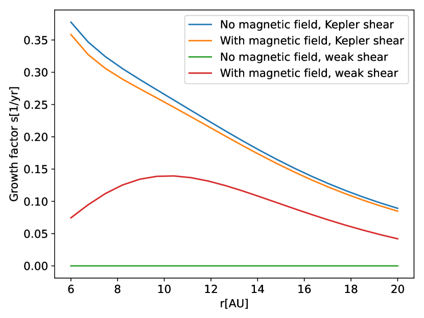
(a) Radial profile of the growth factor $s$ for shearing perturbations obtained from linear perturbation theory for different configurations. Whereas in regions with Keplerian shear, the magnetic field slightly suppresses the perturbations, in the weak-shear case, the magnetic field can destabilize perturbations that would otherwise be stable thus making otherwise stable regions unstable.

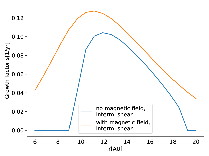
(b) Radial profile of the growth factor $s$ for shearing perturbations obtained from linear perturbation theory for an intermediate shear rate of $\alpha=-0.4$. Such regions appear more frequently in the simulation (see section 4.3). In them, the magnetic field tends to increase the growth rate.

Figure 15: Radial profiles of growth factor $s$ obtained from linear perturbation theory.

In the next step we want to examine the roots of this polynomial $\{\omega_{0}\}$ numerically. In general we expect 4 solutions to the equation. If they are all real, the solution is an oscillating wave. If one of the solutions has an imaginary part, perturbations can grow. Fig. 14(a) in the appendix presents as an example the situation for realistic values at approximately $10\text{AU}$ in a protoplanetary disk. The 4 solutions depending on the wavenumber $k_{y}$ are drawn in different colours where the imaginary part is drawn solid and the real part is dashed. In this case, in the region $k_{y}<5/\text{AU}$ there exists a solution with a non-zero imaginary part which means that perturbations can grow in this regime. At large wavenumbers there is only a real (oscillating) solution.

The next step is now to look if this formalism also shows a destabilizing effect of the magnetic field. For that, a toy model of a protoplanetary disk is introduced, using realistic values comparable to what was used to initialize the simulations from Deng et al. (2021). We now calculate a radial profile of the solution. At each radius, the solutions $\omega_{0}$ of the dispersion relation (21) are calculated for a range of wavenumbers $\vec{k}$ with $\tilde{k}_{x}=0$. At each wavenumber $k_{y}$, the one of the 4 solutions which is growing the fastest is selected. The wavenumber that leads to the largest imaginary part of $\omega$ (which grows the fastest) is then chosen. Its growth factor, defined as $s\coloneqq\mathfrak{Im}(\omega)$, is then taken as the growth factor at this radius (assuming that the fastest growing mode dominates).

Fig. 15(a) shows the growth factor $s$ for different configurations over the radius of the toy model. It shows two situations: One where the shear value is set to the Keplerian shear and another with weak shear where $\alpha=-0.1$. Both situations are shown with and without a magnetic field. In the Keplerian shear situation, the presence of the magnetic field lowers the growth factor a bit. Here, the system is unstable in both cases since the growth factor is non-zero. On the other hand, in the weak shear situation ($\alpha=-0.1$), the magnetic field seems to be required for the system to be unstable. Without the magnetic field (the green line), the growth factor is zero everywhere meaning that the system is stable. When introducing a magnetic field however, the growth-factor is non-zero and thus the system unstable. This is even true when introducing a much weaker magnetic field (10 times smaller) but then the growth factor is also a bit lower. If the magnetic field is further increased in strength, the growth factor seems to saturate. This clearly destabilizing effect seems to be present for shear rates $\alpha\gtrsim-0.15$. In an intermediate regime until ($\alpha\sim-0.4$) (see fig. 15(b)) the magnetic field increases the growth rate but does mostly not destabilize regions that would otherwise be stable.

It is now examined why the magnetic field makes such a difference in the growth factor at low shear. Starting from the dispersion relation (eq. 21) and now assuming zero-shear $\mathcal{A}=0$ one arrives at a quadratic equation in $\nu\coloneqq\omega^{2}$:

$$\begin{split}\nu^{2}\ -\nu\overbrace{\left(\kappa^{2}\ -2\pi G\Sigma\lvert k\rvert+c_{s}^{2}\vec{k}^{2}+k_{x}^{2}\vec{V}_{a}^{2}+k_{y}^{2}(\vec{V}_{a,y}^{2}-\vec{V}_{a,x}^{2})\right)}^{\eqqcolon q}\\ +\underbrace{(k_{x}^{2}V_{a,x}^{2}+k_{y}^{2}V_{a,y}^{2})\left(-2\pi G\lvert\vec{k}\rvert\Sigma+c_{s}^{2}\vec{k}^{2}\right)}_{\eqqcolon w}=0\end{split}$$ (22)

If there is no magnetic field, then $w=0$ and a negative solution in $\nu$ exists only if $q<0$ which is just Toomre’s criterion for instability. If $\nu<0$ then there is a solution with $\omega$ purely imaginary which means exponential growth of the perturbation. Note that however now there is $\kappa=2\Omega$ (since $\mathcal{A}=0$) which makes the model stable at all radii. If the model is stable then $Q>1\iff q>0$ (still without the magnetic field). Now imagine introducing even a small magnetic field. It can be seen that there exists always a $\lvert k\rvert$ such that $w<0$. But if that is the case, then the discriminant is positive $\mathcal{D}=q^{2}-4w>0$ meaning that the solutions are real in $\nu$. The solutions are $\nu=\frac{q\pm\sqrt{\mathcal{D}}}{2}$. From $w<0$ it follows that $\sqrt{\mathcal{D}}>q$. Therefore one of the solutions is negative ($\nu>0$). This again means that $\omega$ is purely imaginary and thus the system becomes unstable. In the case of strong shear, where the system is already unstable, the damping effect of the magnetic field can be attributed to the term in $q$ proportional to the Alfvén velocity which acts like a gas pressure.

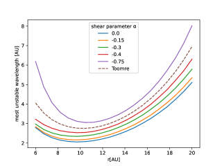
Figure 16: Radial profile of the most unstable wavelength for non-axisymmetric perturbations in a toy model disk with different values of the shear parameter $\alpha$ and including a magnetic field. The Toomre most unstable wavelength is shown as a reference. At weak shear, where the magnetic field may act destabilizing (see fig. 15(a)), the wavelength of the most unstable perturbation is smaller than Toomre’s prediction potentially contributing to the significantly lower size of fragments observed in the MHD simulations.

What are the expected scales of fragmentation? The fastest growing mode for certain values of the shear parameter is plotted in fig. 16. This includes the presence of a magnetic field. It can be seen that the scale is lower for weaker shear meaning that smaller objects may be produced. Compared to the Toomre most unstable wavelength, the scale is somewhat reduced to $2/3$ so it would lead to masses of $1/3$ the size.

When comparing the masses of the clumps in the MHD simulations to the ones from the HD simulation (see fig. 3) one can see that this could explain a large part of the difference between the two cases. Still, the predicted mass is much too large when compared to the clumps actually observed in the simulation. However, when we phenomenologically combine this magnetic destabilization effect with the predicted mass according to (Boley et al., 2010) (see fig. 4) the prediction lies actually in the range of the small clumps from the simulations.

We conclude our discussion of perturbation theory results with a few comments on the validity of the approximations made. With eq. 19 the approximation of a local coordinate system was made. This is only valid if we consider regions that are much smaller than the system’s length scale. This implies that the wavelengths of the perturbation need to be much smaller than the radial distance from the star $\lambda\ll r$. This is certainly fulfilled for the weak-shear cases (see fig. 16). For the strong-shear cases the analysis could become invalid at small radii. Further, the WKB approximation was made where the analysis concentrates on one mode and does not take into account mixing. However, since for non-axisymmetric perturbations the wavenumber $\vec{k}(t)$ is time-dependent this can only be justified as long as the change of $\vec{k}$ is small on the considered time-scale. This means that the growth factor should be large compared to Oort’s parameter, $s\gg k_{x}^{\prime}/\left|\vec{k}\right|=2\left|\mathcal{A}\right|\cdot k_{y}/\left|k\right|\lesssim 2\left|\mathcal{A}\right|$. For the weak-shear case ($\alpha\gtrsim-0.15$) this is also fulfilled over the whole region considered in fig. 15(a) since e.g. at $10\text{AU}$ the angular frequency is $\approx 2\pi/30\text{yr}$ leading to an Oort’s parameter of $\mathcal{A}\approx-0.02/\text{yr}$. However the solutions for non-axisymmetric perturbations at Keplerian shear are probably not valid since then the Oort’s shear parameter is comparable to the growth rate. But still the magnetic field could slightly enhance growth in the regime of intermediate shear $\alpha\gtrsim-0.4$.

From fig. 14(b) one can see that even if we look at the behaviour at later times (here $t=0.5/\Omega$) when the shape of the perturbations has changed (see eq. 20) the solutions to the dispersion relation don’t change much. This means that the time-evolved perturbation is still unstable and can grow further.

After these theoretical considerations it remains to check if the conditions used in this section are met in the simulations. This is done in the next section.

4.3 Preconditions

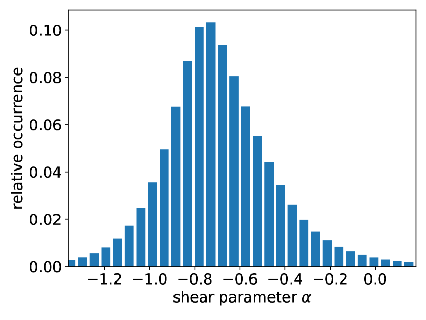
(a) Shear histogram at $t=0$

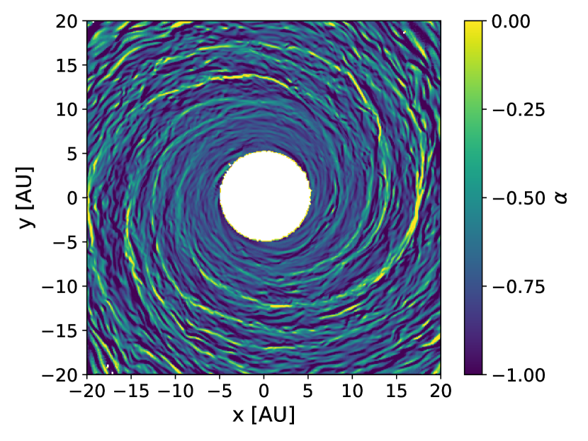
(b) Shear plot at $t=0$

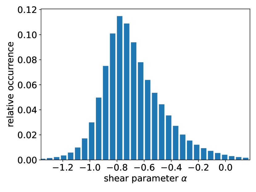
(c) Shear histogram at $t=95\text{yr}$

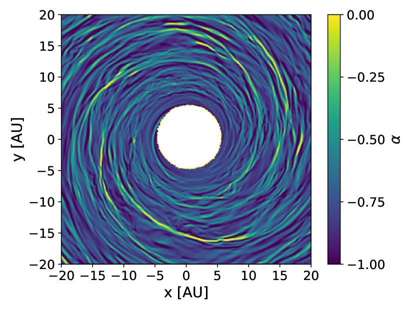
(d) Shear plot at $t=95\text{yr}$

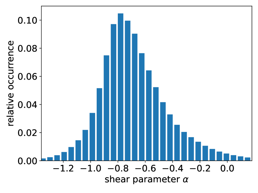
(e) Shear histogram at $t=127\text{yr}$

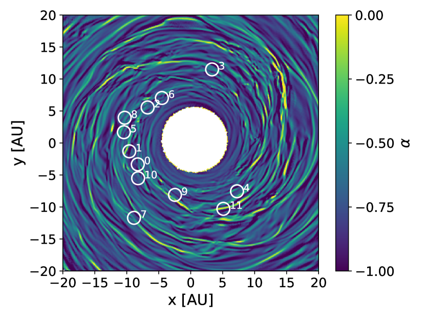
(f) Shear plot at $t=127\text{yr}$

Figure 17: Histogram of values of the shear parameter $\alpha$ at the beginning of the simulation (left column) and color-coded intensity map of the shear parameter in the disk at different times, at the beginning of the simulation (top), right before fragmentation (middle), and after fragmentation (after most clumps have formed (bottom). In the last plot, the locations of the clumps at this time are shown. It is clear that low shear values occur primarily along dense spirals, namely at the typical sites of clump formation.

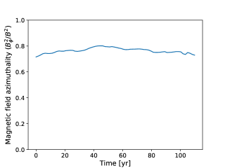
Figure 18: Azimuthality of the magnetic field over the simulation time defined as $B_{\phi}^{2}/B^{2}$ where $B_{\phi}$ is the toroidal part of the magnetic field (relative to the disk) and $B$ the total magnetic field. It is measured taking into account the particles that will later form the clumps and thus traces the collapsing regions.

In the next step we want to find out if the process described in the last section could contribute to the fragmentation results. To this end, we trace the particles of the clumps back in time to compute the physical properties of the fragmenting regions at early stages. The fragmentation process described by Elmegreen (1987) relies on two conditions: First, the magnetic field was assumed to be toroidal such that locally an asymmetry arises between the radial and the azimuthal direction. Second, the effect requires low-shear regions because only then the magnetic field amplifies perturbations and also the size of the perturbations seems to be lower.

Fig. 17 shows the measured shear parameters $\alpha$ in the simulation at various times. It can be seen that most values are around the expected Keplerian shear $\alpha=-0.75$ but there is a wide dispersion. The shear values may deviate from the Keplerian value through gas pressure, turbulence or magnetic field effects. Regions of low shear $\alpha\gtrsim-0.15$ exist, although they are not common ($2\%$). However, regions of intermediate shear $\alpha\gtrsim-0.4$ appear more frequent ($10\%$). In these regions the magnetic field enhances perturbations that would already be unstable without it. Nevertheless, perturbations in regions of these shear values could lead to smaller fragmented objects.

In fig. 18 the relation $B_{\phi}^{2}/B^{2}$ is measured, with $B_{\phi}$ being the azimuthal component of the magnetic field and $B$ the total magnetic field. The relation measures the fraction of the magnetic energy that is in the toroidal component. It is shown over a range of snapshots from the beginning of the simulations until the first fragments appear; only the regions that contain particles that will later fragment are taken into account. It can be seen that the magnetic field is predominantly toroidal but a significant fraction of the energy is also in the radial and the z-component. We assume that this is still compatible with the effect described by Elmegreen because the magnetic field would still be coupled to the contraction much more in the azimuthal direction than in the other directions and could thus still suppress the Coriolis force (see section 4.1). When querying the solutions of the dispersion relation (section 4.2) we arrive at very similar solutions if we don’t use a perfectly axisymmetric magnetic field ($B_{x}=0$).

5 Summary and concluding discussion

As in conventional disk instability, clumps in magnetized self-gravitating disks formed from fragmentation sites inside spiral structure. The flow state in such a disk has been shown to be more turbulent relative to non-magnetized disks, due to a combination of Maxwell and gravitational stresses (Deng et al., 2020), which also leads to more flocculent spiral structure. The initial properties and structure of the clumps in the fragmenting sites are thus determined by a combination of the gas flows kinematics, the magnetic field, and the thermodynamical state of the medium. We analyzed both the pre-collapse and post-collapse properties of the fluid that ends up generating the clumps, which led to numerous findings on the origin, dynamics and development of magnetized clumps:

• Clumps forming in magnetized disks have gravitationally bound masses from one to almost two orders of magnitude lower than clumps in unmagnetized disks, being typically in the range of Super-Earths and Neptune-sized bodies.

• When comparing the energy scales at the time right before the formation of the clumps it is found that the magnetic energy is smaller than the internal energy but dominates over the kinetic turbulence energy. Since the energy stored in the magnetic field is much greater than that in the turbulent motion of particles its role in determining directly the properties and dynamics of clumps is most important.

• After the collapse, the magnetic field is amplified around and inside the clumps. The peak may be just outside the bound radius in which case the magnetic field acts compressing inwards and pushes the surrounding flow outwards, or it can be at the centre of the clump in which case it could just isolate the clump from the outside. In general, we confirm that this ”magnetic shield” stifles gas accretion, suppressing further clump growth.

• While the magnetic field may have its maximum field strength inside the clump, relative to the other energy components, it is dominant only at the periphery of the clumps.

• Thermal gas pressure plays an important role in determining the clump energetics. It is higher than both rotational energy and the magnetic energy near the centre of the clumps. The importance of the magnetic field generally increases further outside, around the bound radius of the clumps.

• After clump formation, rotational energy becomes the dominant form of kinetic energy inside clumps. In their outermost regions clumps are rotationally supported in both MHD and HD simulations, but rotation is significantly higher in the HD clumps than in MHD clumps. As a result the MHD clumps have a lower specific angular momentum than the HD clumps, which brings their spin in better agreement with the spin of gas and ice giant planets in the Solar System (excessively high spins are a known problem for conventional HD fragmentation simulations (Mayer et al., 2004)).

• Beside influencing the evolution of the clumps, the magnetic field also has an influence on the fragmentation process itself being responsible for significantly smaller initial masses of the clumps. Adapting previous results of linear perturbation theory for non-axisymmetric perturbations of a magnetized rotating sheet by Elmegreen (1987) lends evidence for a destabilizing effect of the magnetic field in low-shear regions which results in a smaller characteristic scale of fragments.

We discussed the fragmentation and early evolution of intermediate-mass protoplanets in the MHD disk. It remains however, to investigate their long-term evolution to establish that such protoplanets really contribute to the observed intermediate-mass planet population. First, such protoplanets need to survive for a sufficiently long time, therefore improving the understanding of migration of such clumps will be crucial to determine their further outcome. Inward-migration may eventually lead to tidal disruption by the host star (Boley et al., 2010). To form gas planets, they have to avoid tidal disruption until they cool enough to undergo their second dynamical collapse due to the dissociation of molecular hydrogen (Helled et al., 2014). To form a solid core, it is crucial for them to accrete dust and form a core sufficiently fast. This would be crucial to explain terrestrial intermediate-mass planets. Even after such processes, the protoplanet can still fall into the star (Helled et al., 2014). Deng et al. (2021) noted that the protoplanets experience migration both in- and outward, hence they will eventually be distributed over a broad radial range. However, the disks were evolved for only $\approx 10$ orbits so the question of migration on longer time scales remains to be investigated. The significantly smaller masses of the clumps in magnetized disks are also expected to have an overall impact on the strength of migration. No runaway migration is expected in the mass range of typical clumps, in contrast with clumps in conventional disk instability simulations (Baruteau et al., 2011; Malik et al., 2015), which should significantly increase the chances of clump survival. Furthermore, the different nature of the background flow could have an impact on the nature of the migration process itself. In Nelson & Papaloizou (2004), who simulated low mass planets in MHD non-self-gravitating disks, it was found that a planet of 3 $M_{\text{earth}}$ would experience random walk migration instead of a monotonic drift because of the high turbulence in the disk. Since the disk in the simulations analysed here (Deng et al., 2021) is 10 times more massive, the same mass ratio between disk and planet would correspond to a mass of $\approx 0.05M_{\text{jup}}$, namely compatible with the typical clump mass in our simulations. Therefore, in addition to the low mass, this is another way clumps in magnetized disks would avoid fast migration and survive.

Further improvements in the understanding of the evolution of such protoplanets could be achieved by implementing additional and more accurate physics. Published hydrodynamical simulations of disk instability provide plenty of hints of what physics should be important. As an example, in Stamatellos (2015) it was found that the inclusion of radiative feedback in the simulations changed the outcome of migration for giant gas planets, namely the outward-migration was prevented and inward-migration also came to a halt because of a gap at the orbit of the planet that arose from the heating of the material that was accreted on to the planet. Likewise, Rowther & Meru (2020) showed how heating of the inner disk can stifle migration of massive clumps. Furthermore, in Nayakshin & Cha (2013) it was shown that radiative feedback may have the effect of slowing the accretion of matter on to the planet therefore reducing its growth; but again this result is for giant planets. Also, in the very few simulations that have included even simple approximations to radiative transfer, such as flux-limited diffusion, it has been shown how clump mass growth is slowed down as their thermal pressure support increases beyond what is predicted by Beta cooling or other simple cooling recipes (Szulágyi et al., 2017). This suggests that also radiative transfer, as well as radiative feedback, should be included in future MHD simulations of self-gravitating disks.

Additionally, the effect of ambipolar diffusion and the Hall effect should be studied. The non-ideal effects should be more important near the mid-plane of the disk as in the outer layers the gas is expected to be ionized by the stellar radiation (Perez-Becker & Chiang, 2011). While Ohmic dissipation, which we have included, is usually dominant in the highest density medium as that inside the clumps, ambipolar diffusion could affect magnetic field dissipation in lower density regions, such as at the periphery of the clumps. For example, it should be investigated if ambipolar diffusion should affect the ”magnetic shield” developed around MHD clumps, which, as we have seen, plays an important role in their overall mass growth, or if it could have an influence on the initial stage of fragmentation (although order of magnitude estimates by Deng et al. (2021) suggest that the dissipation rate should be too low to be dynamically relevant over the short timescales probed by our simulations). Moreover, one could use the simulations presented here as a starting point for additional high-resolution simulations of isolated clumps in order to verify their internal structure and study the collapse of MHD clumps similarly to what has been done for hydrodynamical clumps in Galvagni et al. (2012)

While the MHD simulation used $\approx 30$ million particles, the companion HD simulations that we used as a comparison used only $\approx 3$ million. New HD simulations that used $\approx 30$ million particles have also been conducted starting from the same initial conditions using the procedure described in section 2.1. A quick check revealed not much difference from the lower-resolution HD simulations used in this paper, neither in the number of resulting clumps nor in the angular momentum result (see fig. 11) but we did not analyze them any further.

For the perturbation analysis, we note that since we considered non-axisymmetric modes, their wavenumbers change over time leading to mode mixing. A more accurate treatment would have to take this effect into account as it would impact the fragmentation process. More in general, one could question the use of linear perturbation theory as done in this paper, beginning with the fact that we considered perturbations on a smooth axisymmetric background. In fact, it is well established in the literature (eg. Durisen et al. (2007)) that fragmentation occurs inside spiral arms, namely in a non-axisymmetric, already nonlinear flow. Furthermore, spiral structure typically develops after a transient stage in which ring-like global perturbations arise in the disk (eg. Deng et al. (2017)). With this in mind, Deng & Ogilvie (2022) instead of a smooth disk, considered an already nonlinear ring-like structure as the background state, described by solitary waves. Then, they studied the growth of non-axisymmetric perturbations to the solitary modes, identifying fast growth, which would result in the development of a spiral structure. Note that this is different from the conventional swing amplification mechanism, which assumes that non-axisymmetric waves are already present and can increase their amplitude exponentially when they switch from leading to trailing (Goldreich & Lynden-Bell, 1965). Fragmenting sites would thus correspond to self-gravitating patches in the growing non-axisymmetric pattern, a calculation that should be attempted in the future as it could lend a new, more realistic prediction of the fragmentation scale. Subsequently, such an approach should be extended to include the effect of the magnetic field on the mode growth.

Data Availability

The data files that support our analysis will be made available upon reasonable request.

References

- Alibert et al. (2018) Alibert Y., et al., 2018, Nature Astronomy, 2, 873
- Bae et al. (2022) Bae J., et al., 2022, The Astrophysical Journal Letters, 934, L20
- Baruteau et al. (2011) Baruteau C., Meru F., Paardekooper S. J., 2011, in Alecian G., Belkacem K., Samadi R., Valls-Gabaud D., eds, SF2A-2011: Proceedings of the Annual meeting of the French Society of Astronomy and Astrophysics. pp 459–461
- Binney & Tremaine (2008) Binney J., Tremaine S., 2008, Galactic Dynamics: Second Edition. Princeton Series in Astrophysics, Princeton University Press
- Boley et al. (2010) Boley A. C., Hayfield T., Mayer L., Durisen R. H., 2010, Icarus, 207, 509
- Boss (1997) Boss A. P., 1997, Science, 276, 1836
- Deng & Ogilvie (2022) Deng H., Ogilvie G. I., 2022, The Astrophysical Journal Letters, 934, L19
- Deng et al. (2017) Deng H., Mayer L., Meru F., 2017, The Astrophysical Journal, 847, 43
- Deng et al. (2020) Deng H., Mayer L., Latter H., 2020, The Astrophysical Journal, 891, 154
- Deng et al. (2021) Deng H., Mayer L., Helled R., 2021, Nature Astronomy, 5, 440
- Durisen et al. (2007) Durisen R. H., Boss A. P., Mayer L., Nelson A. F., Quinn T., Rice W. K. M., 2007, in Reipurth B., Jewitt D., Keil K., eds, Protostars and Planets V. p. 607 (arXiv:astro-ph/0603179), doi:10.48550/arXiv.astro-ph/0603179
- Elmegreen (1987) Elmegreen B. G., 1987, ApJ, 312, 626
- Galvagni et al. (2011) Galvagni M., Mayer L., Saha P., 2011, in AAS/Division for Extreme Solar Systems Abstracts. p. 33.06
- Galvagni et al. (2012) Galvagni M., Hayfield T., Boley A., Mayer L., Roškar R., Saha P., 2012, MNRAS, 427, 1725
- Gammie (1996) Gammie C. F., 1996, ApJ, 462, 725
- Gammie (2001) Gammie C. F., 2001, ApJ, 553, 174
- Goldreich & Lynden-Bell (1965) Goldreich P., Lynden-Bell D., 1965, MNRAS, 130, 125
- Helled et al. (2011) Helled R., Anderson J. D., Schubert G., Stevenson D. J., 2011, Icarus, 216, 440
- Helled et al. (2014) Helled R., et al., 2014, in Beuther H., Klessen R. S., Dullemond C. P., Henning T., eds, Protostars and Planets VI. p. 643 (arXiv:1311.1142), doi:10.2458/azu˙uapress˙9780816531240-ch028
- Hopkins (2015) Hopkins P. F., 2015, Monthly Notices of the Royal Astronomical Society, 450, 53
- Hopkins (2016) Hopkins P. F., 2016, MNRAS, 462, 576
- Hopkins & Raives (2016) Hopkins P. F., Raives M. J., 2016, MNRAS, 455, 51
- Kuiper (1951) Kuiper G. P., 1951, Proceedings of the National Academy of Sciences, 37, 1
- Malik et al. (2015) Malik M., Meru F., Mayer L., Meyer M., 2015, ApJ, 802, 56
- Masson et al. (2016) Masson J., Chabrier G., Hennebelle P., Vaytet N., Commerçon B., 2016, A&A, 587, A32
- Mayer et al. (2002) Mayer L., Quinn T., Wadsley J., Stadel J., 2002, Science, 298, 1756
- Mayer et al. (2004) Mayer L., Quinn T., Wadsley J., Stadel J., 2004, The Astrophysical Journal, 609, 1045
- Meru et al. (2017) Meru F., Juhász A., Ilee J. D., Clarke C. J., Rosotti G. P., Booth R. A., 2017, ApJ, 839, L24
- Monaghan (1992) Monaghan J. J., 1992, ARA&A, 30, 543
- Morales et al. (2019) Morales J., et al., 2019, Science (New York, N.Y.), 365, 1441
- Mordasini (2018) Mordasini C., 2018, Planetary Population Synthesis. Springer International Publishing, Cham, pp 2425–2474, doi:10.1007/978-3-319-55333-7˙143, https://doi.org/10.1007/978-3-319-55333-7_143
- NASA Exoplanet Science Institute (2023) NASA Exoplanet Science Institute 2023, NASA Exoplanet Archive, https://exoplanetarchive.ipac.caltech.edu/index.html
- Nayakshin & Cha (2013) Nayakshin S., Cha S.-H., 2013, MNRAS, 435, 2099
- Ndugu et al. (2019) Ndugu N., Bitsch B., Jurua E., 2019, Monthly Notices of the Royal Astronomical Society, 488, 3625
- Nelson & Papaloizou (2004) Nelson R. P., Papaloizou J. C. B., 2004, Monthly Notices of the Royal Astronomical Society, 350, 849
- Nero & Bjorkman (2009) Nero D., Bjorkman J. E., 2009, The Astrophysical Journal, 702, L163
- Ormel (2017) Ormel C. W., 2017, The Emerging Paradigm of Pebble Accretion. Springer International Publishing, Cham, pp 197–228, doi:10.1007/978-3-319-60609-5˙7, https://doi.org/10.1007/978-3-319-60609-5_7
- Perez-Becker & Chiang (2011) Perez-Becker D., Chiang E., 2011, ApJ, 735, 8
- Pérez et al. (2016) Pérez L. M., et al., 2016, Science, 353, 1519
- Podolak et al. (2011) Podolak M., Mayer L., Quinn T., 2011, ApJ, 734, 56
- Pollack et al. (1996) Pollack J. B., Hubickyj O., Bodenheimer P., Lissauer J. J., Podolak M., Greenzweig Y., 1996, Icarus, 124, 62
- Riols & Latter (2018) Riols A., Latter H., 2018, Monthly Notices of the Royal Astronomical Society, 482, 3989
- Riols & Latter (2019) Riols A., Latter H., 2019, MNRAS, 482, 3989
- Riols et al. (2021) Riols A., Xu W., Lesur G., Kunz M. W., Latter H., 2021, Monthly Notices of the Royal Astronomical Society, 506, 1407
- Rowther & Meru (2020) Rowther S., Meru F., 2020, MNRAS, 496, 1598
- Safronov (1972) Safronov V. S., 1972.
- Schlecker, M. et al. (2022) Schlecker, M. et al., 2022, A&A, 664, A180
- Schneider et al. (2011) Schneider J., Dedieu C., Le Sidaner P., Savalle R., Zolotukhin I., 2011, A&A, 532, A79
- Shabram et al. (2011) Shabram M., Boley A., Ford E., 2011, in AAS/Division for Extreme Solar Systems Abstracts. p. 38.04
- Stamatellos (2015) Stamatellos D., 2015, The Astrophysical Journal Letters, 810, L11
- Suzuki et al. (2018) Suzuki D., et al., 2018, ApJ, 869, L34
- Szulágyi et al. (2017) Szulágyi J., Mayer L., Quinn T., 2017, MNRAS, 464, 3158
- Toomre (1964) Toomre A., 1964, ApJ, pp 1217–1238
- Turner et al. (2014) Turner N. J., Fromang S., Gammie C., Klahr H., Lesur G., Wardle M., Bai X. N., 2014, in Beuther H., Klessen R. S., Dullemond C. P., Henning T., eds, Protostars and Planets VI. pp 411–432 (arXiv:1401.7306), doi:10.2458/azu˙uapress˙9780816531240-ch018
- Veronesi et al. (2021) Veronesi B., Paneque-Carreño T., Lodato G., Testi L., Pérez L. M., Bertin G., Hall C., 2021, ApJ, 914, L27
- Zhu & Dong (2021) Zhu W., Dong S., 2021, Annual Review of Astronomy and Astrophysics, 59, 291