Can We Scale Transformers to Predict Parameters of Diverse ImageNet Models?

Abstract

Pretraining a neural network on a large dataset is becoming a cornerstone in machine learning that is within the reach of only a few communities with large-resources. We aim at an ambitious goal of democratizing pretraining. Towards that goal, we train and release a single neural network that can predict high quality ImageNet parameters of other neural networks. By using predicted parameters for initialization we are able to boost training of diverse ImageNet models available in PyTorch. When transferred to other datasets, models initialized with predicted parameters also converge faster and reach competitive final performance.

https://github.com/SamsungSAILMontreal/ghn3

1 Introduction

Training a neural network $f$ initialized with parameters $\mathbf{w}$ is typically done by running a stochastic gradient descent (SGD) optimization algorithm on a dataset $\mathcal{D}$:

$${\mathbf{w}}^{*}=\text{SGD}(f,\mathbf{w},\mathcal{D}).$$ (1)

Novel neural architectures, e.g. Vision Transformer (Dosovitskiy et al., 2020), are usually first pretrained by Eq. (1) on some large $\mathcal{D}$ such as ImageNet (Russakovsky et al., 2015) or, some in-house data such as JFT-300M, and then transferred to other downstream tasks (Kornblith et al., 2019; Zhai et al., 2019; Dosovitskiy et al., 2020). With the growing size of networks $f$ and with multiple runs needed (e.g. for hyperparameter tuning), the cost of pretraining is becoming unsustainable (Strubell et al., 2019; Thompson et al., 2020; Zhai et al., 2022). Therefore, pretraining is becoming one of the key factors increasing the gap between a few privileged communities (often big industries) and many low-resource communities (often academics and small companies).

Figure 1: We introduce GHN-3 models of a significantly larger scale and larger training meta-batch size ($m$) compared to GHN-2 (Knyazev et al., 2021). Scaling up GHNs leads to consistent improvements in the quality of predicted parameters when used as initialization on ImageNet. This plot is based on the accuracies of the PyTorch-10 models in Table 2.

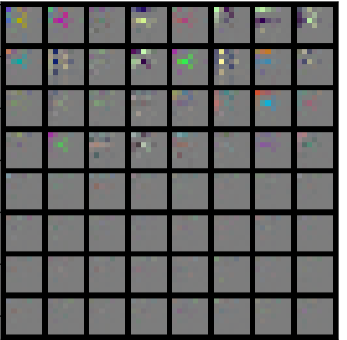
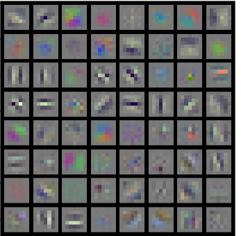
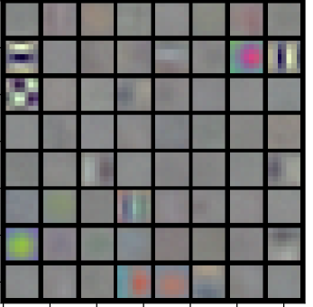
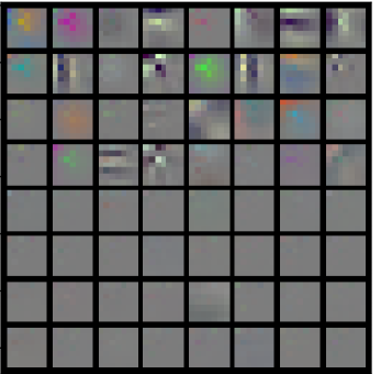
Initialization:	GHN-2	GHN-3-XL/m16 (ours)	Rand init
Parameters trained for:	no training	no training	1 epoch
Time (sec):	0.9 on CPU	1.1 on CPU	$4\times 10^{3}$ on GPU
ImageNet acc:	1.1%	20.0%	18.2%
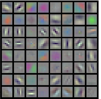
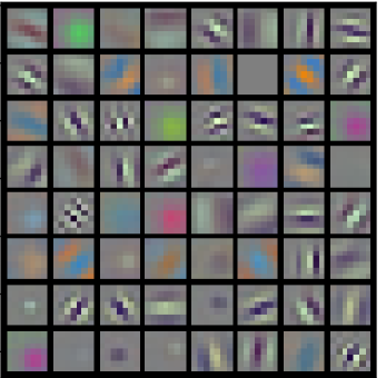
Parameters trained for:	1 epoch	1 epoch	90 epochs
Time (sec):	$4\times 10^{3}$ on GPU	$4\times 10^{3}$ on GPU	$6\times 10^{5}$ on GPU
ImageNet acc:	14.6%	43.7%	76.1%

Figure 2: ResNet-50 first layer parameters predicted with the baseline GHN-2, our GHN-3-XL/m16 and optimized with SGD on ImageNet for 1 and 90 epochs. For the GHNs, ResNet-50 is an unseen architecture, i.e. not present in the training dataset of architectures (Knyazev et al., 2021). The “Time” row shows a rough time estimation to obtain all the parameters of ResNet-50 (for SGD the time is based on Knyazev et al. (2021)). The “ImageNet acc” row shows top-1 validation accuracy on ImageNet ILSVRC-2012. Our GHN-3 predicts parameters as fast as GHN-2, but significantly improves the quality of predicted parameters making their performance higher, fine-tuning easier and visual appearance similar to those trained with SGD for 90 epochs. See Section 5 for experiment details.

We aim at an ambitious goal of democratizing the cost of pretraining. To do so, we follow recent works where one network (HyperNetwork) parameterized by $\theta$ is trained to predict good parameters $\mathbf{w}_{\text{pred}}$ for unseen network architectures $f$ (Zhang et al., 2018; Knyazev et al., 2021; Shang et al., 2022) or datasets $\mathcal{D}$ (Zhmoginov et al., 2022). We focus in this paper on generalization to new architectures $f$ in a large-scale ImageNet setting so that the HyperNetwork $H_{\mathcal{D}}$ is used as:

$$\mathbf{w}_{\text{pred}}=H_{\mathcal{D}}(f,\theta).$$ (2)

We use the parameters $\mathbf{w}_{\text{pred}}$ predicted on ImageNet ($\mathcal{D}$) as initialization, so by fine-tuning them on $\mathcal{D}$ we can reduce pretraining cost or we can transfer them to another dataset $\mathcal{D}^{\text{transfer}}$ by fine-tuning them on $\mathcal{D}^{\text{transfer}}$ with Eq. (1):

$${\mathbf{w}}^{*}=\text{SGD}(f,\mathbf{w}_{\text{pred}},\mathcal{D}\ \text{or}\ \mathcal{D}^{\text{transfer}}).$$ (3)

While training $H_{\mathcal{D}}$ is more expensive than training $f$ from scratch, we train $H_{\mathcal{D}}$ only once and publicly release it to move towards democratized pretraining. This way, new architectures (including very large ones) designed by different research communities may be boosted “for free” by initializing them with $\mathbf{w}_{\text{pred}}$ by a simple forward pass through $H_{\mathcal{D}}$. Our proposed $H_{\mathcal{D}}$ is built on Graph HyperNetworks (GHNs) (Zhang et al., 2018), in particular GHN-2  (Knyazev et al., 2021) which previously often fell short to improve over random initializations. The GHN-3 we introduce predicts parameters of a significantly better quality (Fig. 2). We make the following contributions:

1. We adopt Transformer from Ying et al. (2021) to improve the efficiency and scalability of GHNs and we modify it to better capture local and global graph structure of neural architectures (Section 4);

2. We significantly scale up our Transformer-based GHN (GHN-3) and we release our largest model achieving the best results at https://github.com/SamsungSAILMontreal/ghn3 (Fig. 1);

3. We evaluate GHNs by predicting parameters for around 1000 unseen ImageNet models, including all models available in the official PyTorch framework (Paszke et al., 2019). Despite such a challenging setting, our GHN-3 shows high quality and performance and can significantly improve training of neural networks on ImageNet and other vision tasks (Section 5).

2 Related Work

Parameter prediction. Parameter prediction or generation is often done by hypernetworks (Ha et al., 2016). Originally, hypernetworks were able to generate model parameters only for a specific architecture and dataset. Several works extended them to generalize to unseen architectures (Brock et al., 2017; Zhang et al., 2018) and datasets (Requeima et al., 2019; Zhmoginov et al., 2022). We focus on the unseen architectures regime where the most performant and flexible method so far is graph hypernetworks (GHNs) (Zhang et al., 2018). Knyazev et al. (2021) improved GHNs by introducing GHN-2 predicting parameters for unseen architectures with relatively high performance in image classification tasks. To train and evaluate GHNs, they introduced a diverse and large dataset of training and evaluation architectures – DeepNets-1M. Our proposed GHN-3 closely resembles GHN-2 and uses the same training dataset. However, GHN-3 is $>100\times$ larger, which we show is important to increase the performance on ImageNet. At the same time, GHN-3 is efficient during training (and comparable during inference, see Fig. 2) due to using transformer layers as opposed to a slow GatedGNN of GHN-2 that required sequential graph traversal (Section 3).

Generative models of neural networks. Another line of work is based on first collecting a dataset of trained networks and then learning a generative model by fitting the distribution of trained weights. Schürholt et al. (2022) train an auto-encoder with a bottleneck representation with the ability to sample new weights. Peebles et al. (2022) train a generative diffusion transformer to generate weights conditioned on random initialization for the same architecture and dataset. Ashkenazi et al. (2022) improve the quality of generated parameters by combining hypernetworks and generative models, but their model is architecture-specific and unable to generate weights for unseen architectures as GHNs.

Data-driven initialization. GHNs can be viewed as a data-driven initialization method. Predicted parameters are generally inferior than those trained with SGD for many epochs, so using the predicted ones as initialization (Eq. 2) followed by fine-tuning with SGD (Eq. 3) is a logical approach. GradInit (Zhu et al., 2021) and MetaInit (Dauphin & Schoenholz, 2019) are methods to initialize a given neural network on a given dataset by adjusting the weights to improve the gradient flow properties. Neural initialization optimization (NIO) (Yang et al., 2022) further improves on them. These methods generally outperform a standard random-based initialization (He et al., 2015) and carefully designed architecture-specific initialization rules (Zhang et al., 2019). Compared to these, in our work the initial parameters are predicted by a GHN given a computational graph of the neural network. Our approach leverages a million of training architectures making the predicted parameters better for initialization as we show. Another recent initialization method (Czyzewski et al., 2022) requires a source network and the quality of the initialization depends on how similar are the source and target networks. Their work is related to Net2Net (Chen et al., 2015) and GradMax (Evci et al., 2022) that require a smaller variant of the network or a certain growing scheduler. Our GHN-based approach is more flexible as we can initialize a larger variety of networks without the need of source networks or growing schedules. Additional related work is also discussed in Section A.4.1.

3 Background

3.1 Graph HyperNetworks

A Graph HyperNetwork (GHN) (Zhang et al., 2018; Knyazev et al., 2021) is a neural network $H_{\mathcal{D}}$ parameterized by $\theta$ and trained on a dataset $\mathcal{D}$. The input to the GHN is a computational graph $f^{G}$ of a neural network $f$; the output is its parameters $\mathbf{w}_{\text{pred}}$: $\mathbf{w}_{\text{pred}}=H_{\mathcal{D}}(f^{G};{\theta})$. In our context, $\mathcal{D}$ can be an ImageNet classification task, $f$ can be ResNet-50 while $\mathbf{w}_{\text{pred}}$ are parameters of ResNet-50’s convolutional, batch normalization and classification layers. Knyazev et al. (2021) train the GHN $H_{D}$ by running SGD on the following optimization problem over $M$ training architectures $\{f^{G}_{a}\}_{a=1}^{M}$ and $N$ training samples $\{\mathbf{x}_{j},y_{j}\}_{j=1}^{N}$:

$$\underset{\theta}{\text{arg\,min }}\frac{1}{NM}\sum_{j=1}^{N}\sum_{a=1}^{M}\mathcal{L}\Big{(}f_{a}\Big{(}\mathbf{x}_{j};H_{\mathcal{D}}(f^{G}_{a};{\theta})\Big{)},y_{j}\Big{)}.$$ (4)

During training $H_{D}$, a meta-batch of $m$ training architectures is sampled for which $H_{D}$ predicts parameters. Simultaneously, a mini-batch of $b$ training samples $\mathbf{x}$ is sampled and forward propagated through the predicted parameters for $m$ architectures to predict $m\times b$ sample labels $\hat{y}$. For classification, the cross-entropy loss $\mathcal{L}$ is computed between $\hat{y}$ and ground truth labels $y$ of $\mathbf{x}$, after which the loss is backpropagated to update the parameters $\theta$ of $H_{D}$ with gradient descent. In GHN-2 and in this work, training architectures are sampled from DeepNets-1M – a dataset of 1 million architectures (Knyazev et al., 2021). Training samples $\mathbf{x}$ represent images and $y$ are their labels.

The input computational graph $f^{G}=(V,E)$ is a directed acyclic graph (DAG), where the nodes $V$ correspond to operations (convolution, pooling, self-attention, etc.), while the edges $E$ correspond to the forward pass flow of inputs through the network $f$. GHNs take $d$-dimensional node features $\mathbf{H}^{(1)}\in\mathbb{R}^{|V|\times d}$ as input obtained using an embedding layer for each $i$-th node: $\mathbf{h}^{(1)}_{i}=\text{Embed}(\mathbf{h}^{(0)}_{i})$, where $\mathbf{h}^{(0)}_{i}$ is a one-hot vector denoting an operation (e.g. convolution). The graph $f^{G}$ is traversed in the forward and backward directions and features $\mathbf{H}^{(1)}$ are sequentially updated using a gated graph neural network (GatedGNN) (Li et al., 2015). After the GatedGNN updates node features, the decoder uses them to predict the parameter tensor of the predefined shape. In GHN-2, this shape is equal to $2d{\mkern-0.1mu\times\mkern-0.1mu}2d{\mkern-0.1mu\times\mkern-0.1mu}16{\mkern-0.1mu\times\mkern-0.1mu}16$. The final predicted parameters $\mathbf{w}_{\text{pred}}$ associated with each node are obtained by copying or slicing this tensor as necessary.

3.2 Transformers

Transformers are neural networks with a series of self-attention (SA)-based layers applied to $d$-dimensional features $\mathbf{H}\in\mathbb{R}^{n\times d}$ (Vaswani et al., 2017). In a Transformer layer, SA projects $\mathbf{H}$ using learnable parameters $\mathbf{W}_{Q},\mathbf{W}_{K},\mathbf{W}_{V}$ followed by the pairwise dot product, softmax and another dot product (for simplicity we omit the layer superscript ^(l) in our notation unless necessary):

$$Q =\mathbf{H}\mathbf{W}_{Q},K=\mathbf{H}\mathbf{W}_{K},V=\ \mathbf{H}\mathbf{W}_{V},$$ (5)

$$\mathbf{A} =\frac{\mathbf{Q}\mathbf{K}^{T}}{\sqrt{d}},\ \ \text{SA}(\mathbf{H})=\ \text{softmax}(\mathbf{A})\mathbf{V}.$$ (6)

A Transformer layer consists of multi-head SA (MSA) with $k$ heads, and a series of fully-connected and normalization layers (Vaswani et al., 2017; Dosovitskiy et al., 2020).

3.3 Transformers on Graphs

A vanilla Transformer defined above can in principle be applied to graph features $\mathbf{H}^{(1)}\in\mathbb{R}^{|V|\times d}$, but it does not have ingredients to capture the graph structure (edges). Several variants of Transformer layers on graphs have been proposed (Dwivedi & Bresson, 2020; Ying et al., 2021; Kim et al., 2022; Chen et al., 2022). We rely on Graphormers (Ying et al., 2021) due to its simplicity and strong ability to capture local and global graph structure. In Graphormers, node features are augmented with node degree (centrality) embeddings. For directed graphs, such as DAGs, these are in-degree $\mathbf{z}_{\text{deg}^{+}(i)}$ and out-degree embeddings $\mathbf{z}_{\text{deg}^{-}(i)}$, so an embedding $\mathbf{h}^{(1)}_{i}$ for the $i$-th node is defined as:

$$\mathbf{h}^{(1)}_{i}=\text{Embed}(\mathbf{h}^{(0)}_{i})+\mathbf{z}_{\text{deg}^{+}(i)}+\mathbf{z}_{\text{deg}^{-}(i)},$$ (7)

where $\text{Embed}(\mathbf{h}^{(0)}_{i})$ are some initial node embeddings, e.g. see in Section 3.1. When self-attention in Eq. (6) is applied to graphs, we can interpret $\mathbf{A}_{ij}$ as a scalar encoding the relationship between nodes $i$ and $j$. To incorporate the graph structure in Transformers, Graphormer layers add an edge embedding $\mathbf{e}(i,j)$ to $\mathbf{A}_{ij}$ in self-attention:

$$\mathbf{\tilde{A}}_{ij}=\frac{(\mathbf{h}_{i}\mathbf{W}_{Q})(\mathbf{h}_{j}\mathbf{W}_{K})^{T}}{\sqrt{d}}+\mathbf{e}(i,j),$$ (8)

where $\mathbf{\tilde{A}}$ replaces $\mathbf{A}$ in Eq. (6) without changing the other components of the Transformer layer. Graphormers model $\mathbf{e}(i,j)$ as a learnable scalar dependant on the shortest path distance between nodes $i$ and $j$, shared across all Graphormer layers. While for SA $\mathbf{e}(i,j)$ is a scalar, for MSA $\mathbf{e}(i,j)$ is a vector of length equal to the number of heads $k$. See further details in (Ying et al., 2021).

4 Scalable Graph HyperNetworks: GHN-3

Our GHN-3 model modifies GHN-2 (Knyazev et al., 2021) in three key ways: (1) replacing a GatedGNN with Graphormer-based layers; (2) improving the training loss of GHNs; (3) increasing the scale and meta-batch of GHNs.

4.1 Transformer on Computational Graphs

In GHN-3, we replace a GatedGNN with a stack of $L$ Graphormer-based layers built based on Eq. (8) and applied to $\mathbf{H}^{(1)}$ defined in Eq. (7). Since the information in computational graphs can flow in the forward ($i\rightarrow j$) and backward ($j\rightarrow i$) directions, we explicitly separate edge embeddings into two terms, so that our self-attention is based on:

$$\mathbf{\tilde{A}}_{ij}=\frac{(\mathbf{h}_{i}\mathbf{W}_{Q})(\mathbf{h}_{j}\mathbf{W}_{K})^{T}}{\sqrt{d}}+\phi([\mathbf{e}(i,j),\mathbf{e}(j,i)]).$$ (9)

where $\phi$ is a series of fully connected layers. While in principle multiple Graphormer layers (Eq. 8) could infer that the backward pass is the inverse of the forward pass, we found that explicitly separating the embeddings and adding $\phi$ facilitates learning as we confirm in Ablations (Section 5).

4.2 Predicted Parameter Regularization

Knyazev et al. (2021) showed that the parameters predicted by GHNs can lead to a higher variance of activations compared to the variances of activations for parameters optimized with SGD (see their Appendix B). Too high variances may lead to instabilities during training GHNs as well as to negative effects in applications. For example, if such predicted parameters are used for initialization, their fine-tuning can be challenging. To alleviate this issue, we add a group $\ell_{1}\!-\!\ell_{2}$ regularization (Scardapane et al., 2017) on the predicted parameters $\mathbf{w}_{\text{pred}}$ during training GHN-3, so that the total GHN-3 training loss becomes:

$$\mathcal{L}=\mathcal{L}_{CE}+\gamma\sum\nolimits_{i}||\mathbf{w}_{\text{pred},i}||_{2},$$ (10)

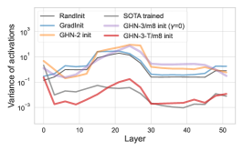
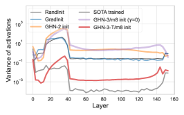
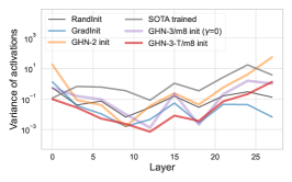
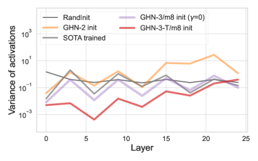
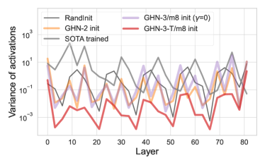
where $\mathcal{L}_{CE}$ is the cross-entropy loss (same as in the baseline GHN-2), $\gamma$ is a tunable coefficient controlling the strength of the penalty and $i$ is the layer index of the training neural network $f_{a}$ (see Eq. 4). Our regularization encourages smaller values in predicted parameters and consequently smaller variances of activations that are expected to be more aligned with the activations of models trained with SGD (see Fig. 6-bottom). Besides Eq. (10), we also experimented with other forms of regularization including $\sum\nolimits_{i}\mathbf{w}_{\text{pred},i}^{2}$, but Eq. (10) overall worked the best (see ablations in Table 5).

4.3 Increased Scale

Once we replace GatedGNN with Graphormer-based layers, scaling up GHNs becomes straightforward by increasing the number of the Graphormer-based layers $L$ and hidden size $d$. The decoder of our GHN-3 has the same architecture as in GHN-2 with the hidden size increasing proportionally to $d$ (see Appendix A.1). The decoder takes the output node features of the last Graphormer layer to predict parameters. In contrast to our approach, scaling up GHN-2 is not trivial since a single GatedGNN layer is computationally expensive as it requires sequential graph traversal, so stacking such layers is not feasible (see Section 5). Instead, Graphormer layers update all node features in parallel making our GHN-3 efficient and scalable. Increasing the meta-batch size $m$ (see Section 3.1) is also straightforward, so when training a GHN on $g$ GPU devices, each device processes $m/g$ architectures and the gradients of the GHN parameters $\theta$ are averaged on the main device (Knyazev et al., 2021).

Despite the simple modifications outlined in this Section, GHN-3 brings GHNs to a significantly better level in the quality of predicted parameters with important practical implications as we empirically show next.

5 Experiments

We evaluate if neural networks initialized with the parameters $\mathbf{w}_{\text{pred}}$ predicted by GHNs obtain high performance without any training (Eq. 2) and after fine-tuning (Eq. 3). We focus on a large-scale ImageNet setting, but also evaluate in a transfer learning setting from ImageNet to few-shot image classification and object detection tasks.

Training GHN-3. We train the GHNs on the ILSVRC-2012 ImageNet dataset (Russakovsky et al., 2015) with 1.28M training and 50K validation images of the 1k classes. All GHNs are trained for 75 epochs using AdamW (Loshchilov & Hutter, 2017), initial learning rate 4e-4 decayed using the cosine scheduling, weight decay $\lambda$=1e-2, predicted parameter regularization $\gamma$=3e-5 (Eq. 10), batch size $b$=128 and automatic mixed precision in PyTorch (Paszke et al., 2019). We train the GHNs on the same training split of 1 million architectures, DeepNets-1M, used to train GHN-2 (Knyazev et al., 2021).

GHN-3 variants. We train GHN-3 models of four scales (Table 1). We begin with a tiny scale GHN-3-T that has the same order of parameters (6.9M) as GHN-2 (2.3M). We then gradually increase the number of layers, hidden size and heads in the Graphormer-based layers following a common style in Transformers (Dosovitskiy et al., 2020; Liu et al., 2021). We train all variants with meta-batch size $m$=8 and 16 and denote the GHNs with the /m8 and /m16 suffixes.

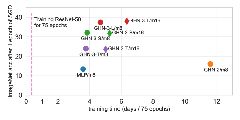
Efficient distributed implementation. We build on the open-source implementation of GHN-2 (Knyazev et al., 2021) and improve its efficiency by using a distributed training pipeline and removing redundant computations. Our implementation reduces the training time of GHNs by around 50% (see Appendix A.3). However, despite our best efforts GHN-2 still takes more than 11 days to train (Fig. 3). Larger versions of GHN-2, e.g. by stacking two GatedGNN layers, are estimated to require $>$ 20 days making it expensive to train. In contrast, our GHN-3 is significantly faster to train while achieving stronger results (Fig. 3). For example, one of our best performing models (GHN-3-L/m16) is about $2{\mkern-0.1mu\times\mkern-0.1mu}$ faster to train and is more than 2${\mkern-0.1mu\times\mkern-0.1mu}$ better in accuracy. The cost of training our GHNs is still higher than training a single network (e.g. full training of ResNet-50 takes about 0.4 days on 4xNVIDIA-A100). However, we train each GHN only once and we publicly release them, so that they can predict parameters for many diverse and large ImageNet models in $\approx 1$ second even on a CPU (Fig. 2).

Table 1: Details of GHNs. Train time is for GHNs with $m=8$ and is measured on 4xNVIDIA-A100 GPUs. ^*GHN-3-XL requires 8 GPUs, so its training time is not directly comparable. GHN-2-S is a larger version of the baseline GHN-2 that we attempted to train but were unable to complete due to poor training efficiency.

Name	Layers $L$	Hidden size $d$	Heads $k$	Params	Train time
GHN-2	1	32	$-$	2.3M	11.5 days
GHN-2-S	2	128	$-$	35.0M	20.5 days
GHN-3-T	3	64	8	6.9M	3.7 days
GHN-3-S	5	128	16	35.8M	3.8 days
GHN-3-L	12	256	16	214.7M	4.7 days
GHN-3-XL	24	384	16	654.4M	4.8* days

Figure 3: ImageNet accuracy of fine-tuning predicted parameters vs training speed of GHNs. Our GHN-3 is efficient to train and at the same time the predicted parameters achieve higher accuracy. All measurements are made on 4xNVIDIA-A100 GPUs.

Baselines. Our main baselines are GHN-2, released by Knyazev et al. (2021), random initialization (RandInit) implemented by default in PyTorch, typically based on He et al. (2015). In full training experiments, we also compare our approach to more advanced initializations, GradInit (Zhu et al., 2021) and NIO (Yang et al., 2022). For reference, we also compare to the SOTA results reported in prior literature. However, this baseline is not a fair comparison since it requires 90-600 epochs of training on ImageNet and often relies on advanced optimization algorithms, augmentations and other numerous tricks.

Evaluation architectures. For evaluation of GHNs we use two splits of neural network architectures. (1) The evaluation splits of DeepNets-1M: 900 in-distribution (Test split) and out-of-distribution (Wide, Deep, Dense and BN-Free splits) architectures (Knyazev et al., 2021). (2) PyTorch: 74 architectures for which trained ImageNet weights are available in PyTorch-v1.13 (Paszke et al., 2019). As shown by Knyazev et al. (2021), all the evaluation architectures of DeepNets-1M are different from the ones used to train GHNs. The architectures of PyTorch are even more different, diverse and on average of a significantly larger scale than the ones in DeepNets-1M (Table 3).

Table 2: ImageNet top-1 accuracy (%) after predicting parameters and fine-tuning them for 1/10 (1k SGD steps) and 1 (10k steps) epoch. Average and standard deviation of accuracies for top-10 networks in the DeepNets-1M and PyTorch splits are reported. SOTA results denote accuracies reported in the official PyTorch documentation and require 90-600 epochs, advanced optimizers and numerous tricks.

Initialization	No fine-tuning		1/10 epoch of SGD		1 epoch of SGD		SOTA
	deepnets1-1m-10	pytorch-10	deepnets1-1m-10	pytorch-10	deepnets1-1m-10	pytorch-10	pytorch-10
RandInit	0.2$\pm$0.0	0.2$\pm$0.0	5.2$\pm$0.7	1.1$\pm$0.3	34.7$\pm$1.1	25.9$\pm$1.3	84.2$\pm$0.7
GHN-2/m8	24.6$\pm$0.4	0.7$\pm$0.4	15.9$\pm$1.3	7.6$\pm$2.7	24.9$\pm$1.3	16.0$\pm$3.2	90-600 epochs
GHN-3-T/m8	31.3$\pm$0.3	3.9$\pm$3.9	31.9$\pm$1.9	15.3$\pm$3.4	33.6$\pm$1.5	23.9$\pm$1.0
GHN-3-T/m16	30.0$\pm$0.2	5.3$\pm$4.5	31.6$\pm$1.1	16.1$\pm$3.8	32.8$\pm$1.0	23.6$\pm$1.6
GHN-3-S/m8	41.1$\pm$0.7	6.0$\pm$6.3	42.1$\pm$1.8	22.5$\pm$5.0	43.4$\pm$1.5	32.1$\pm$1.4
GHN-3-S/m16	41.3$\pm$0.6	7.8$\pm$7.0	41.9$\pm$2.5	22.0$\pm$5.9	43.5$\pm$1.7	31.8$\pm$2.0
GHN-3-L/m8	43.6$\pm$1.0	10.7$\pm$9.3	44.0$\pm$2.8	26.2$\pm$5.1	46.0$\pm$2.0	37.4$\pm$1.9
GHN-3-L/m16	44.7$\pm$0.7	9.8$\pm$8.1	42.9$\pm$5.6	27.3$\pm$4.6	46.4$\pm$3.1	38.0$\pm$2.3
GHN-3-XL/m8	43.8$\pm$0.8	8.5$\pm$8.1	45.7$\pm$2.5	28.2$\pm$6.1	47.5$\pm$2.3	36.9$\pm$3.8
GHN-3-XL/m16	47.1$\pm$0.9	11.5$\pm$8.4	48.1$\pm$3.7	30.6$\pm$7.2	50.1$\pm$3.0	40.3$\pm$3.9

Figure 4: ImageNet results for all PyTorch models after 1 and 10 epochs of SGD, and after SOTA training for at least 90 epochs. The left and right figures show the models for which GHN-3-XL/m16+SGD-1ep outperforms and underperforms RandInit+SGD-1ep. See accuracies and rank correlation results in Table 20.

Table 3: The evaluation splits of neural architectures. The average, standard deviation and range of property values are shown. Graph degrees and paths are computed based on Knyazev et al. (2021).

Eval. split	nets	params (M)	Graph degree	Graph path
DeepNets-1M	900	9$\pm$16 (2.2 - 102)	2.3$\pm$0.1 (2.1 - 2.8)	15$\pm$7 (5.1 - 72)
PyTorch	74	56$\pm$64 (1.2 - 307)	2.5$\pm$1.2 (1.9 - 9.1)	16$\pm$6 (6.8 - 37)

5.1 Experiments on DeepNets-1M and PyTorch

Setup. Using trained GHNs we first predict ImageNet parameters for all 900 + 74 evaluation architectures in DeepNets-1M and PyTorch and evaluate their ImageNet classification accuracy (top-1) by propagating validation images. We then initialize the networks (1) with parameters predicted by GHNs or (2) randomly (RandInit), and fine-tune them using SGD on ImageNet to compare convergence dynamics between (1) and (2). Since fine-tuning all the 974 networks for all initialization approaches is prohibitive, we choose top-10 networks in each split, denoted as DeepNets-1M-10 and PyTorch-10 respectively. For the GHNs, the top-10 networks are chosen based on the accuracy obtained by directly evaluating (no fine-tuning) predicted parameters on ImageNet. For RandInit, the top-10 networks are chosen based on the network accuracy after 1 epoch of SGD (denoted as SGD-1ep). For DeepNets-1M, the accuracies of RandInit+SGD-1ep are taken from (Knyazev et al., 2021). For PyTorch we trained all networks for 1 epoch using SGD with a range of learning rates (0.4, 0.1, 0.04, 0.01, 0.001), momentum 0.9, weight decay 3e-5 and batch size 128. We choose the networks achieving the best validation accuracy among all the learning rates and report the average accuracy (Table 2). For the GHNs, we fine-tune top-10 networks initialized with predicted parameters using SGD for 1 epoch using the same range of hyperparameters as for training from RandInit. For our best GHN-3-XL/m16 we also fine-tune all PyTorch networks.

Table 4: Summary of the results presented in Fig. 4. “Wins” denotes a fraction of networks for which a GHN-3-based init. outperformed RandInit+SGD-1ep. “Avg gain/loss” denotes an average gain/loss versus RandInit+SGD-1ep when GHN-3 wins/loses.

Method	Wins	Avg gain	Avg loss
GHN-3-XL/m16 no fine-tune	5%	1.6%	-16.4%
GHN-3-XL/m16 + SGD-1/10ep	14%	11.0%	-12.0%
GHN-3-XL/m16 + SGD-1ep	74%	12.3%	-4.2%

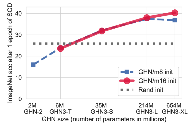
Results of fine-tuning top-10 models for 1 epoch. As reported in Table 2, our GHN-3-based initialization consistently improves ImageNet performance compared to RandInit and the GHN-2-based initialization for all training regimes and for both DeepNets-1M-10 and PyTorch-10 architecture splits. Moreover, GHN-3 results gracefully improve with the GHN scale. For larger GHN-3 models, increasing meta-batch size ($m$) is important. For example, when $m$ is increased from 8 to 16, ImageNet accuracy on PyTorch-10 after 1 epoch increases by 3.4 points for GHN-3-XL versus a -0.3 point decrease for GHN-3-T. The overall trend indicates that further increase of the GHN-3 scale and meta-batch size should yield more gains (Fig. 1). Our best model, GHN-3-XL/m16, when used as an initializer for PyTorch-10 models leads to fast convergence. For example, after fine-tuning predicted parameters for just 1/10 epoch (1k SGD steps) we achieve 30.6% while RandInit achieves only 1.1% after 1/10 epoch and 25.9% after 1 epoch. The GHN-2-based initialization is considerably worse than RandInit leading to 16.0% after 1 epoch. Thus, our GHN-3 models and in particular GHN-3-XL/m16 make a major step from GHN-2 by making GHNs useful for initialization.

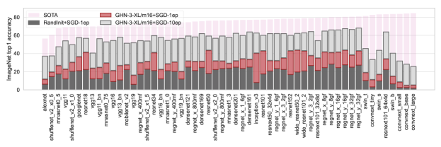
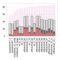
Results of fine-tuning all PyTorch models for 1-10 epochs. Using our best model, GHN-3-XL/m16, we initialized and then fine-tuned for 1 epoch all 74 PyTorch models and compared to RandInit (Fig. 4). GHN-3-XL/m16 improves RandInit in 74% (55 out of 74) cases with an average accuracy gain of 12.3% in absolute points (Table 4, Fig. 4-left). While our initialization is inferior in 26% cases, the accuracy drop is relatively small and is -4.2% on average (Table 4, Fig. 4-right). Most of the lost cases correspond to the networks with a squeeze and excitation operation (EfficientNet, MobileNet), indicating a potential problem of GHNs to predict good parameters in that case. Nevertheless, when fine-tuning for 10 epochs, all PyTorch models initialized using GHN-3-XL/m16 improve their performance fast and in some cases approach SOTA training from RandInit for $\geq$90 epochs. For example, RegNet-y-32gf achieves 68% after 10 epochs outperforming six SOTA-trained models.

Ablations. We study which components of GHN-3, besides the scale and meta-batch size, are important for the performance. To do so, we apply our previous setup from Table 2 to ablated GHN-3-T/m8 models (Table 5). First, we show that our predicted parameter regularization (Eq. 10) is important. It explicitly enforces smaller values in predicted parameters which facilitates their fine-tuning (Fig. 6). Second, adding separate edge embeddings for the backward pass of computational graphs (Eq. 9) also improves results (from 20.4% to 23.9%) with almost no increase in the GHN size. Finally, the accuracy drops the most when edge embeddings and self-attention are removed. Self-attention without edge embeddings (Eq. 6) still allows for the exchange of information between the nodes of graphs, therefore the accuracy is not as low (18.9%) as when self-attention is removed (13.4%). These last two results confirm the importance of capturing the graph structure of neural architectures and that our GHN-3 is an effective model to achieve that. Additional ablations are shown and discussed in Appendix A.2.

Table 5: Ablations. ImageNet validation accuracy after 1 training epoch for the PyTorch-10 models initialized with GHN-3-T/m8.

Model	SA	FW	BW	$\gamma$	Params	Acc
GHN-3-T/m8	✓	✓	✓	3e-5	6.91M	23.9$\pm$1.0
$\gamma\sum\nolimits_{i}\mathbf{w}_{\text{pred},i}^{2}$ reg. in Eq. (10)	✓	✓	✓	3e-5	6.91M	22.5$\pm$2.2
No pred. par. reg. in Eq. (10)	✓	✓	✓	0	6.91M	19.9$\pm$4.7
No bw embed. in Eq. (9)	✓	✓	✗	3e-5	6.90M	20.4$\pm$6.9
No egde embed., SA Eq. (6)	✓	✗	✗	3e-5	6.88M	18.9$\pm$4.1
No egde embed., MLP	✗	✗	✗	3e-5	6.74M	13.4$\pm$0.8

Figure 5: Generalization results of GHNs without fine-tuning predicted parameters on five evaluation splits of DeepNets-1M using ImageNet accuracy. The number in parentheses indicates the number of architectures in each split. See the numerical results for these and other GHNs in Table 11 in Appendix.

ResNet-50	ResNet-152	Swin Transformer (Swin-T)

Figure 6: (top) Validation accuracy curves of ResNet-50, ResNet-152 and Swin-T on ImageNet. See the training accuracy curves in Fig. 8 in Appendix. Standard learning rate schedules are used for ResNets (decay every 30 epochs) and Swin-T (cosine decay). (bottom) Variance of activations in the networks initialized with the methods we compare (see Section 5.4 for the details).

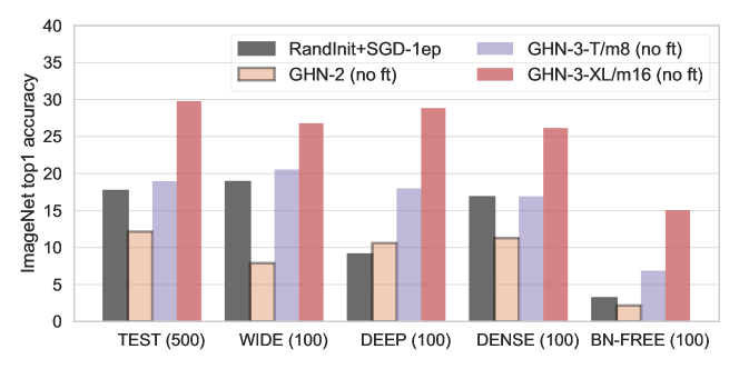
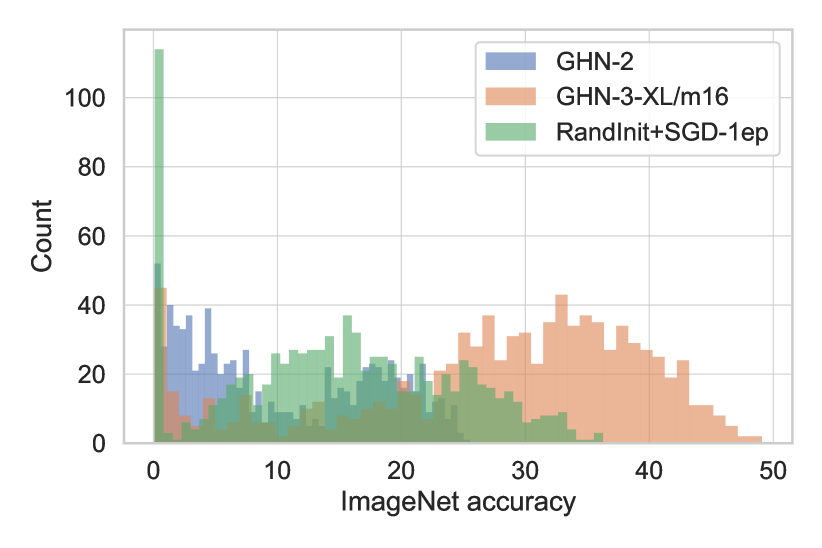
Generalization. When predicted parameters are evaluated without fine-tuning, GHN-2 showed good generalization to unseen architectures of DeepNets-1M, including the out-of-distribution splits: Wide, Deep, Dense and BN-Free (Knyazev et al., 2021). However, the performance of GHN-2 is still lower compared to RandInit+SGD-1ep (Fig. 5). Our GHN-3-XL/m16 without any fine-tuning not only matches but outperforms training with SGD for 1 epoch on all evaluations splits of DeepNets-1M by a large margin.

5.2 Full Training

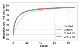
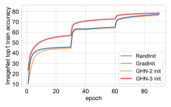
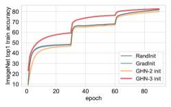
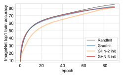
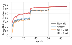
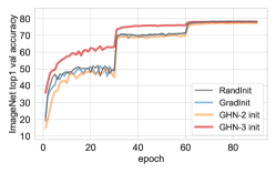
Setup. We explore if the benefits of a GHN-3-based initialization still hold when the networks are trained for many epochs as in SOTA training. We compare the GHN-3-XL/m16-based initialization to GHN-2, RandInit and stronger initialization baselines, GradInit (Zhu et al., 2021) and NIO (Yang et al., 2022). We consider three architectures, ResNet-50, ResNet-152 (He et al., 2016) and Swin Transformer (Liu et al., 2021) (its tiny variant denoted as Swin-T), achieving strong performance in vision tasks. We use standard training settings for ResNets: 90 epochs of SGD with momentum 0.9 and batch size 128. A standard (well-tuned) initial learning rate 0.1 is used for RandInit, GradInit and NIO, while for GHN-based initializations we perform light tuning of the initial learning rate among (0.1, 0.025, 0.01), since predicted parameters may need only slight fine-tuning. In all cases, the learning rate is decayed every 30 epochs. For Swin-T we follow Liu et al. (2021) and train with AdamW and the cosine learning rate scheduling, but use computationally light settings to make training feasible. In particular, we use batch size 512 and train for 90 epochs and only using standard augmentation methods as for the ResNets. For Swin-T each initialization method is tuned: initial learning rate is chosen from (1e-3, 6e-4, 3e-4) and the weight decay from (0.01, 0.05). For all the networks when using the GHN initialization, to break the symmetry of identical parameters, we add a small amount of noise with $\beta$=1e-5 to all parameters following Knyazev (2022). We repeat training runs for 3 random seeds in all cases.

Table 6: Comparison of initialization methods for ResNet-50, ResNet-152 and Swin-T on ImageNet. Average accuracies over 3 runs are reported. For all methods, a standard deviation after 1 epoch is $\leq 2$, after 45 epochs is $\leq 0.3$ and after 90 epochs is $\leq 0.1$. Initialization time is measured on 1xNVIDIA-A100 in seconds; average time over the three networks is reported. We also compare to FixUp (Zhang et al., 2019) in Table 16.

Init.	Init.	ResNet-50				ResNet-152				Swin-T
method	time	1 ep	45 ep	90 ep		1 ep	45 ep	90 ep		1 ep	45 ep	90 ep
RandInit	0.2	20.6	67.3	76.0		19.7	70.5	78.2		18.4	72.7	75.6
GradInit	1700	21.1	67.9	76.2		22.5	70.5	78.2		20.3	72.1	75.0
NIO	85	21.0	68.1	76.1		$-$	$-$	$-$		$-$	$-$	$-$
GHN-2	1.3	12.8	66.5	75.6		13.9	69.2	77.4		15.8	70.3	75.8
GHN-3	1.2	35.0	73.5	76.2		34.3	75.9	78.1		27.1	73.7	76.4

Results. As shown in Fig. 6-top and Table 6, our GHN-3-based initialization speeds up convergence for all the three networks compared to all other initialization methods, including GradInit and NIO. The gap between our GHN-3 and others is especially high during the first few epochs and particularly for ResNets. After training for longer, the gap between the methods gradually shrinks and all the initialization methods show comparable performance with two exceptions. First, on Swin-T the final accuracy of our GHN-3-based initialization is noticeably better than all other methods (76.4% vs 75.8% of the best baseline). Second, the baseline GHN-2 is generally worse than other initialization methods converging slowly and underperforming at the end. Overall, our GHN-3 brings GHNs to a significantly better level by improving convergence versus other methods in the first epochs. Advanced initialization methods, NIO and GradInit, performed similarly to each other in our ResNet-50 experiments, and we were unable to run NIO for the other networks (Table 6). Compared to NIO and GradInit, GHN-3 has an extra advantage besides converging faster in the beginning. Specifically, NIO and GradInit require propagating and computing gradients for 100-2000 mini-batches on ImageNet to initialize each network, which can be inconvenient in practice (Zhu et al., 2021; Yang et al., 2022). In contrast, our trained GHN-3 predicts ImageNet parameters for each network in $\approx$ 1 second (even on a CPU) and without accessing ImageNet.

Modern training recipes. While we used standard training recipes with 90 epochs, modern training recipes require up to 600 epochs with stronger regularizations and other tricks to reach higher accuracy at a higher computational cost (Wightman et al., 2021). However, the goal of this work is not to achieve SOTA at a high cost, but to achieve competitive performance at a low computational cost (in a few epochs) by leveraging GHN-3. As we report in Table 6, the final 90 epoch accuracies of the GHN-3-based initialization are generally similar to RandInit and we expect this trend to maintain if the modern recipes are used.

5.3 Transfer Learning

Setup. We explore if the parameters predicted by our GHNs for ImageNet can be transferred to other tasks. We consider three architectures: ResNet-50, Swin-T and the base variant of ConvNeXt (Liu et al., 2022). We compare the following initialization approaches: (1) RandInit, (2) orthogonal initialization (Saxe et al., 2013), (3) parameters predicted by GHNs, (4) RandInit or predicted parameters trained/fine-tuned on ImageNet for 1 epoch and (5) RandInit trained on ImageNet for 90-600 epochs. The latter requires significant computational resources and therefore is not considered to be a fair baseline. We fine-tune the networks initialized with one of these approaches on the few-shot variants of the CIFAR-10 and CIFAR-100 image classification tasks (Krizhevsky et al., 2009). Following (Zhai et al., 2019; Knyazev et al., 2021) we consider 1000 training samples in each task, which is well suited to study transfer learning abilities. To transfer ImageNet parameters to CIFAR-10 and CIFAR-100, we re-initialize the classification layer with RandInit with 10 and 100 outputs respectively and fine-tune the entire network. We tune hyperparameters for each method in a fair fashion following (Knyazev, 2022). We also evaluate on the Penn-Fudan object detection task (Wang et al., 2007) containing only 170 images. We closely follow the setup and hyperparameters from (Knyazev et al., 2021; PyTorchTutorial, ) and evaluate on three common backbones, ResNet-50, ResNet-101 and ResNet-152 (He et al., 2016). In all cases, we repeat experiments 3 times and report an average and standard deviation.

Table 7: Transfer learning from ImageNet to few-shot CIFAR-10 and CIFAR-100 with 1000 training labels with 3 networks: ResNet-50 (R-50), ConvNext-B (C-B) and Swin-T (S-T). Average accuracies over 3 runs are reported; std in all cases is generally $\leq$ 0.5.

Initialization	ImageNet	CIFAR-10			CIFAR-100
	pretrain	R-50	C-B	S-T	R-50	C-B	S-T
RandInit	No	61.6	48.0	46.0	14.5	11.6	12.2
Orth	No	61.1	52.4	47.8	14.8	13.6	12.5
GHN-2	No	61.8	52.3	48.2	18.3	13.7	12.7
GHN-3-XL/m16	No	72.9	55.3	51.8	27.8	13.8	11.9
RandInit	1 epoch	74.0	69.1	62.1	33.1	19.9	24.2
GHN-2	1 epoch	68.4	69.1	58.6	26.6	28.0	21.4
GHN-3-XL/m16	1 epoch	77.8	71.3	64.3	37.2	31.0	26.5
RandInit	90-600 ep	88.7	95.6	93.4	56.1	69.7	62.5

Table 8: Transfer learning results (average precision at IoU=0.50 measured in %) for the Penn-Fudan object detection dataset.

Initialization	ImNet pretr.	ResNet-50	ResNet-101	ResNet-152
RandInit	No	21.3$\pm$4.9	14.9$\pm$1.1	18.4$\pm$1.9
GHN-2	No	54.9$\pm$1.4	55.1$\pm$3.2	55.8$\pm$5.7
GHN-3-XL/m16	No	61.7$\pm$3.8	60.2$\pm$7.6	60.0$\pm$5.2
RandInit	90 epochs	87.6$\pm$1.1	88.2$\pm$4.8	89.3$\pm$5.1

Results. The parameters predicted by our GHNs show better transferability compared to GHN-2 in all but one of the transfer learning experiments (Tables 7 and 8). We also significantly improve on RandInit. By fine-tuning the predicted parameters on ImageNet for 1 epoch before transferring them to the CIFAR datasets we achieve further boosts and outperform RandInit+SGD-1ep. While the gap with full ImageNet pretraining is still noticeable (e.g. 77.8% vs 88.7% for ResNet-50 on CIFAR-10), we narrow this gap compared to GHN-2 (68.4%) and RandInit (74.0%).

5.4 Qualitative Analysis and Discussion

We analyze the diversity of predicted parameters following experiments in (Knyazev et al., 2021). We predict parameters for all PyTorch models and from them collect all the parameter tensors of one of the three frequently occurring shapes. We then compute the absolute cosine distance between all pairs of parameter tensors of the same shape and report the mean of the pairwise matrix (Table 9). In general the parameters predicted by our GHN-3 are more diverse than the ones predicted by GHN-2 even though we did not enforce the diversity during training GHN-3. One exception is parameters of the shape $64{\mkern-0.1mu\times\mkern-0.1mu}3{\mkern-0.1mu\times\mkern-0.1mu}7{\mkern-0.1mu\times\mkern-0.1mu}7$ used in the first convolutional layer of many models. However, in both GHN-2 and GHN-3 the diversity of this tensor is small, while GHN-3 improves the quality visually (Fig. 2).

We also evaluate the quality of predicted parameters by computing the variance of activations when propagating a mini-batch of images through the network. We initialize the networks with random-based methods, SOTA trained parameters or parameters predicted by GHNs and propagate the same mini-batch of images through the network to compute activations and their variances (Fig. 6-bottom). For the ResNets, the GHN-3 initialization leads to the variances well aligned with SOTA trained models. Our predicted parameter regularization (Section 4.2) is important to enable this behavior. However, our activations are not always well aligned with pretrained models as we show for ViT and EfficientNet (Fig. 9 in Appendix), which may explain a lower fine-tuning accuracy for these networks (Fig. 4-right).

Finally, GHNs can be used to efficiently estimate the performance of architectures making them a potentially useful approach for neural architecture search (NAS). However, GHNs are not explicitly trained to perform the NAS task and in our experiments underperformed compared to other NAS methods (Appendix A.4). At the same time, our GHN-3-XL/m16 outperformed GHN-2 and a smaller scale GHN-3 indicating the promise of large-scale GHNs for NAS.

We provide additional results and discussion in Appendix A.

Table 9: Diversity of the parameters predicted by GHNs vs SOTA trained by SGD from RandInit measured on the PyTorch split. ^*Since the parameters in the SOTA trained models are not ordered in a canonical way, we employ the Hungarian matching (Kuhn, 1955) before computing the distance between a pair of tensors.

Method	Parameter tensor shape
	$64{\mkern-0.1mu\times\mkern-0.1mu}3{\mkern-0.1mu\times\mkern-0.1mu}7{\mkern-0.1mu\times\mkern-0.1mu}7$	$256{\mkern-0.1mu\times\mkern-0.1mu}256{\mkern-0.1mu\times\mkern-0.1mu}3{\mkern-0.1mu\times\mkern-0.1mu}3$	$1024{\mkern-0.1mu\times\mkern-0.1mu}1024{\mkern-0.1mu\times\mkern-0.1mu}1{\mkern-0.1mu\times\mkern-0.1mu}1$
MLP	0.0	0.174	0.020
GHN-2	1e-3	0.283	0.070
GHN-3-XL/m16	2e-4	0.310	0.095
SOTA training*	0.388	0.917	0.895

6 Conclusion

We improve Graph HyperNetworks by considerably scaling them up. By evaluating on realistic and challenging ImageNet architectures, we found that scaling up gradually increases the overall performance. This is encouraging as further scaling GHNs can make them a powerful tool. Our GHN-3 improves random-based and advanced initializations in vision experiments and makes a big step in the quality of predicted parameters compared to the prior GHNs.

Appendix A APPENDIX

A.1 GHN Details

The decoder of our GHN-3 has the same architecture as in GHN-2, however when we scale GHN-3 we set the final output dimensionality of the decoder to $d{\mkern-0.1mu\times\mkern-0.1mu}d{\mkern-0.1mu\times\mkern-0.1mu}16{\mkern-0.1mu\times\mkern-0.1mu}16$ instead of $2d{\mkern-0.1mu\times\mkern-0.1mu}2d{\mkern-0.1mu\times\mkern-0.1mu}16{\mkern-0.1mu\times\mkern-0.1mu}16$. This final output dimensionality determines the maximum size of the predicted parameter tensor and larger/smaller tensors are obtained by tiling/slicing the largest one following the implementation in (Knyazev et al., 2021). See Section A.3 for an empirical analysis of this design choice.

In addition to the in-degree and out-degree (centrality) node embeddings (Eq. 7) our GHN-3 models add one extra embedding to nodes. In particular, to each node we add the embedding corresponding to the distance from the input node $i=0$. This embedding is not important for our results, and we empirically analyze the usefulness of the centrality and input distance embeddings in Section A.3.

For a few recent architectures (e.g. ConvNeXt) in the PyTorch split, some layers are not supported by GHNs (not available during training). We do not predict the parameters of those layers and use standard initialization for them.

A.2 Predicted Parameter Regularization Ablations

Alternatively to applying our predicted parameter regularization (Eq. 10), it is possible to apply a higher weight decay $\lambda$ on the GHN parameters to implicitly enforce it predict smaller values. We verified that increasing $\lambda$ by a factor of 10 only slightly improved the results of the GHN with $\gamma$=0 (from 19.9% to 21.3%, see Table 10), while further increasing $\lambda$ to 0.3 worsens results (from 19.9% to 18.9%). The results with increased $\lambda$ confirm the advantage of explicitly regularizing predicted parameters (23.9%). Tuning $\gamma$ is also important and using a larger value (1e-4 instead of 3e-5) worsens results (20.0% vs 23.9%).

Table 10: Additional ablation results following Table 5.

Model	Params	Acc
GHN-3-T/m8 ($\gamma$=3e-5, $\lambda$=0.01)	6.91M	23.9$\pm$1.0
No predicted param. reg. ($\gamma$=0) in Eq. (10)	6.91M	19.9$\pm$4.7
No predicted param. reg. ($\gamma$=0) in Eq. (10), $\lambda$=0.1	6.91M	21.3$\pm$1.9
No predicted param. reg. ($\gamma$=0) in Eq. (10), $\lambda$=0.3	6.91M	18.9$\pm$1.1
Predicted param. reg. $\gamma$=1e-4 in Eq. (10)	6.91M	20.0$\pm$3.0

A.3 Additional Results

A.3.1 Additional GHN variants

In Table 11 we report the results for more GHN variants on DeepNets-1M without fine-tuning predicted parameters.

First, we retrained GHN-2 using our implementation and hyperparameters (see iii in Table 11), including predicted parameter regularization (Eq.10). It performed slightly better than the GHN-2 released by Knyazev et al. (2021) (ii) implying that our hyperparameters (optimizer, learning rate, etc.) are preferable. At the same time, due to our implementation improvements it takes two times less time to train it. We also trained a smaller variant of our GHN-3-T (iv) with the same hidden size $d$ and same decoder output shape ($2d{\mkern-0.1mu\times\mkern-0.1mu}2d{\mkern-0.1mu\times\mkern-0.1mu}16{\mkern-0.1mu\times\mkern-0.1mu}16$) as in GHN-2, which has a comparable number of trainable parameters as the baseline GHN-2. This GHN-3 variant performs slightly better than the retrained GHN-2, but takes 3.5 times less time to train than GHN-2 (iii).

We also trained GHN-2 with a larger hidden size ($d$=128, seex in Table 11), which has about the same number of parameters as our GHN-3-S (xii). It performed worse than GHN-3-S and is about three times longer to train. Overall, GHN-3 is much faster to train than GHN-2 and is more performant due to a deep Graphormer-based architecture rather than a shallow GatedGNN-based architecture. These two factors allow us to scale up GHN-3 and obtain significant improvements. We also compared GHN-3-T with our default output dimensionality $d{\mkern-0.1mu\times\mkern-0.1mu}d{\mkern-0.1mu\times\mkern-0.1mu}16{\mkern-0.1mu\times\mkern-0.1mu}16$ (xii) to a GHN with a larger output dimensionality, $4d{\mkern-0.1mu\times\mkern-0.1mu}4d{\mkern-0.1mu\times\mkern-0.1mu}16{\mkern-0.1mu\times\mkern-0.1mu}16$ (xi). The latter performed worse compared to GHN-3-S with around the same number of parameters validating our approach to scale up GHNs.

Finally, we evaluate a GHN without centrality node embeddings introduced in Graphormers (Eq. 7) and found that its usefulness is limited (see v and vii in Table 11). Regarding the input distance embedding (Section A.1), we found it to be useful in the initial experiments. However similarly to the centrality embedding, in our final experiments it provided only marginal gains compared to the GHN-3-T without the input distance embedding (see v and vii). At the same time, these node embeddings become very useful when edge embeddings are removed (see viii and ix and vii). Apparently, these node embeddings provide some noisy information about the graph structure, but this information becomes less useful when edge embeddings are added. Since both the centrality and input distance embeddings do not introduce significantly more trainable parameters or computational demands while provide small gains in some cases, we keep them in our final GHNs.

A.3.2 Results summary

Table 12 reports the results of GHNs vs RandInit on all 900 + 74 evaluation networks without and with fine-tuning. These results summarize the histograms in Fig. 4. The distribution of accuracies on DeepNets-1M is shown in Fig. 7.

Table 11: Generalization results on the evaluation architecture splits of DeepNets-1M using ImageNet top-1 accuracy. ^*Days on 4xNVIDIA-A100 for 75 epochs. ^**Days on 8xNVIDIA-A100 for 75 epochs.

#	Method	SGD steps	Params (M)	Train time*	Test	Wide	Deep	Dense	BN-free	All
	# architectures				500	100	100	100	100	900
(i)	RandInit	10k (1ep)	$-$	$-$	17.7$\pm$7.7	18.9$\pm$9.9	9.1$\pm$7.3	16.8$\pm$7.7	3.2$\pm$5.2	15.1$\pm$9.2
(ii)	GHN-2/m8	0	2.32	21.9	12.1$\pm$7.6	7.9$\pm$7.2	10.6$\pm$7.1	11.3$\pm$6.7	2.2$\pm$1.9	10.3$\pm$7.6
(iii)	GHN-2/m8 (our implem. and hyperparams and Eq.(10))	0	2.32	11.6	14.3$\pm$6.5	15.2$\pm$6.4	12.7$\pm$6.5	12.2$\pm$6.5	2.9$\pm$3.0	12.7$\pm$7.2
(iv)	GHN-3/m8 ($d=32$, decoder output: $2d{\mkern-0.1mu\times\mkern-0.1mu}2d{\mkern-0.1mu\times\mkern-0.1mu}16{\mkern-0.1mu\times\mkern-0.1mu}16$)	0	2.37	3.2	14.3$\pm$7.4	15.5$\pm$7.3	13.0$\pm$6.8	12.8$\pm$6.7	2.1$\pm$2.4	12.8$\pm$7.9
(v)	GHN-3-T/m8-no centr. embed. (Eq. 7)	0	6.89	3.8	18.6$\pm$7.7	20.2$\pm$7.4	17.8$\pm$7.7	16.9$\pm$8.1	6.4$\pm$3.6	17.1$\pm$8.3
(vi)	GHN-3-T/m8-no input dist. embed. (Section A.1)	0	6.84	3.8	19.0$\pm$7.7	20.1$\pm$8.2	18.0$\pm$7.9	17.0$\pm$8.4	6.5$\pm$3.8	17.4$\pm$8.5
(vii)	GHN-3-T/m8	0	6.91	3.8	19.0$\pm$7.6	20.5$\pm$7.5	18.0$\pm$7.7	16.9$\pm$8.3	6.9$\pm$4.1	17.5$\pm$8.3
(viii)	GHN-3-T/m8, No fw/bw embed. in Eq. (9)	0	6.88	3.7	14.7$\pm$6.5	15.3$\pm$7.0	13.5$\pm$6.2	13.0$\pm$6.6	4.4$\pm$3.8	13.3$\pm$7.1
(ix)	GHN-3-T/m8, No fw/bw/centr/input dist. embed	0	6.80	3.7	10.2$\pm$5.5	9.5$\pm$6.0	9.5$\pm$4.8	9.3$\pm$4.8	4.0$\pm$3.0	9.3$\pm$5.5
(x)	GHN-2/m8 ($d$=128) (our implem. and hyperparams)	0	34.73	11.9	22.4$\pm$9.8	22.2$\pm$11.3	21.7$\pm$9.3	18.5$\pm$9.9	6.8$\pm$6.0	20.1$\pm$10.8
(xi)	GHN-3-T/m8 (decoder output: $4d{\mkern-0.1mu\times\mkern-0.1mu}4d{\mkern-0.1mu\times\mkern-0.1mu}16{\mkern-0.1mu\times\mkern-0.1mu}16$)	0	38.86	3.8	23.9$\pm$10.8	21.5$\pm$13.7	22.9$\pm$9.6	20.2$\pm$10.5	7.6$\pm$6.2	21.3$\pm$11.7
(xii)	GHN-3-S/m8	0	35.81	3.8	24.2$\pm$10.0	25.7$\pm$11.3	23.8$\pm$9.5	21.2$\pm$10.1	10.3$\pm$5.2	22.4$\pm$10.7
(xiii)	GHN-3-XL/m16	0	654.37	7.1**	29.8$\pm$11.2	26.8$\pm$15.6	28.8$\pm$9.5	26.2$\pm$10.9	15.1$\pm$9.7	27.3$\pm$12.3

Table 12: ImageNet top-1 accuracy for all 900 + 74 evaluations networks in DeepNets-1M and PyTorch. Average and standard deviation of accuracies for all networks in each split are reported.

	SGD steps	DeepNets-1M	PyTorch
GHN-2	0	10.3$\pm$7.6	0.2$\pm$0.3
GHN-3-XL/m16	0	27.3$\pm$12.3	1.7$\pm$5.0
RandInit	10k (1ep)	15.1$\pm$9.2	17.4$\pm$7.2
GHN-3-XL/m16	1k (1/10ep)	$-$	8.3$\pm$10.2
GHN-3-XL/m16	10k (1ep)	$-$	25.4$\pm$12.3

Figure 7: ImageNet top-1 accuracy on all the 900 architectures of DeepNets-1M for GHNs without fine-tuning vs RandInit+SGD-1ep.

A.3.3 Huge ResNet and ViT

The main value of our GHN-3 is in strong initialization for many networks that do not have ImageNet weights. For example, for all the 900 evaluation architectures in DeepNets-1M there are no pretrained ImageNet weights and our GHN-3 achieves strong results for them (see Table 12). To further support our argument, we show that we can predict good parameters for huge ResNet-1000 with $>$ 400M parameters and ViT-1.2B with $>$ 1.2 billion parameters (the ViT is based on the “no distribution shift” experiment described in Section A.3.4). No pretrained weights are available for them. We train them for 1 epoch (due to high cost) with RandInit and our GHN-3 init. using two learning rates. We found that GHN-3 can initialize well such huge networks despite being trained on much smaller ones (Table 13). On average, our GHN-3 init is better for both the 0.1 and 0.01 learning rates and both architectures, in some cases by a large margin, further confirming the strength of our GHN in such a challenging setting. Potentially, this can lead to significant cost reductions. GHN-3 also provides more stable gradient norm at initialization (very large gradient norm of RandInit for ResNet-1000 may lead to numerical overflow and training instabilities). Finally, the GHN-3-based initialization can be less sensitive to the learning rate (also see Table 18 for additional learning rate sensitivity results).

Table 13: ImageNet top-1 accuracy for huge ResNet and ViT after 1 epoch of training (averaged for 3 runs).

Model	Init.	initial grad norm	1 epoch
			lr=0.1	lr=0.01
ResNet-1000	RandInit	99121.9	21.0$\pm$1.0	15.5$\pm$0.7
	GHN-3	72.0	23.1$\pm$1.9	32.2$\pm$1.1
ViT-1.2B	RandInit	4.8	2.0$\pm$0.5	16.5$\pm$0.3
	GHN-3	6.9	11.8$\pm$0.8	17.4$\pm$0.6

A.3.4 Architecture distribution shift

For some PyTorch architectures, in particular ViT and EfficientNet, there is a certain distribution shift from the DeepNets-1M training architectures used to train GHNs and their specification in PyTorch.

We focus on ViT and EfficientNet as concrete examples:

• ViT: ViTs in PyTorch use a classification token, which is never used in the DeepNets-1M architectures. In DeepNets-1M, global average pooling (GAP) is used instead to obtain the last layer features.

• EfficientNet: EfficientNets in PyTorch have a squeeze and excitation operation with a SiLU activation, while in DeepNets-1M only ReLU is used in those layers.

These distribution shifts can be fixed by either including a PyTorch based classification token and SiLU in the DeepNets-1M training set or by slightly adjusting ViT/EfficientNet architectures in PyTorch. To support our argument, we follow the latter approach. For ViT we replace the classification token with GAP, while for EfficientNet we replace SiLU with ReLU. We report the results after 1 epoch with distr. shift (original PyTorch architectures) and no distr. shift (our adjusted architectures) in Table 14. We show that when the distribution shift is removed, the GHN-based initialization outperforms RandInit. We note that the distribution shift issue is inherent to neural network based methods and it is likely to come up with examples where a neural net fails. We did not alter the original PyTorch ViT/EfficientNet architectures in our main experiments in Table 2 to show this limitation of GHNs. But here we show that the distribution shift problem can be mitigated if needed. We believe future work can focus on designing more diverse training architectures than DeepNets-1M, so that the issue of the distribution shift is less pronounced.

Table 14: ImageNet top-1 accuracy for ViT/EfficientNet with and without the distribution shift.

Model	Init. method	With distr. shift	No distr. shift
ViT-B/16	RandInit	11.06	9.87
	GHN-3	8.49	11.47
EfficientNet-B0	RandInit	24.64	23.29
	GHN-3	22.19	32.00

A.3.5 Ensembling

We evaluated if the predicted parameters of different architectures can be ensembled to improve performance. We chose three networks for which GHN-3 predicts the parameters that achieve good accuracy without any training (Table 15). We construct an ensemble by averaging the logits from the three networks when we propagate the validation images of ImageNet. As another experiment, we also fine-tuned the three networks with SGD for 1 epoch and ensembled them to see how the results change after fine-tuning. We compare to the baseline GHN-2, MLP, GHN-3-T (our tiny GHN-3) and RandInit. We report the validation accuracy of individual networks and their ensemble (Table 15). We found that our best model (GHN-3) predicts somewhat diverse parameters as the results of the ensemble slightly improve even without any training. While the baselines (GHN-2, MLP and GHN-3-T) do no gain from ensembling, it may or may not be due to less diverse parameters. Evaluation of ensembles of predicted parameters is challenging, because some networks with predicted parameters can be of very poor quality weakening the ensemble. Therefore, we also evaluated the ensemble after fine-tuning predicted parameters which have a smaller variance of accuracy. RandInit gains the most from ensembling, perhaps because RandInit leads to more diverse parameters (see Table 9). However, GHN-3+SGD-1ep is still much stronger than RandInit+SGD-1ep in terms of final performance with 48.39 vs 27.45. We believe large ensembles of GHN-3+SGD-1ep networks is a promising avenue for future research.

Table 15: Ensembling results on ImageNet (top-1 accuracy).

Method	Resnet-50	ResNet-101	Wide-Resnet-101	Ensemble
GHN-2	1.08	1.46	0.70	1.06
MLP	2.52	1.91	2.51	2.61
GHN-3-T	10.59	5.41	6.17	8.63
GHN-3	19.92	18.86	18.60	21.07
RandInit+SGD-1ep	16.63	20.46	19.97	27.45
GHN-3+SGD-1ep	43.33	42.61	43.11	48.39

A.3.6 Comparison to FixUp

Methods such as FixUp (Zhang et al., 2019) provide better initialization than RandInit in some cases and so they are related to our work. We compare to FixUp in Table 16 using ResNet-50 without batch normalization. Our GHN-3 based initialization significantly improves convergence compared to FixUp and all the other initializations by a large margin (Table 16). In addition, our GHN-3 has a broader scope improving initialization for the networks with batch norm as well (Table 6), whereas FixUp and normalization-free networks are focused on training the networks without batch norm and do not improve results with batch norm.

Table 16: Comparison of initialization methods for ResNet-50 without batch normalization on ImageNet after 1 epoch of training.

Init. method	Init. time	1 epoch
RandInit	0.2	10.8
GradInit	1700	19.2
FixUp	0.2	18.0
GHN-2	1.3	5.9
GHN-3	1.2	31.7

A.3.7 Choice of optimizers

Depending on the optimizer, different initialization methods may be more performant. To study that, we train Swin-T with AdamW (as in Section 5.2) and SGD with momentum and compare our GHN-3-based initialization to RandInit after 1 epoch of training (Table 17). The results show better performance of our GHN-3 in all cases.

Table 17: ImageNet top-1 accuracy of Swin-T after 1 epoch for different optimizers and initializations.

Init. method	AdamW	SGD (lr=0.05)	SGD (lr=0.025)	SGD (lr=0.01)
RandInit	18.4	12.7	10.6	6.8
GHN-3	27.1	19.4	19.2	16.1

A.3.8 Learning rate sensitivity

An intriguing question to ask is: does initializing ImageNet models using GHN-3 makes them more robust to hyperparameters? To verify this, we computed the fraction of networks (%) in the PyTorch split for which the best accuracy (after 1 epoch) can be achieved using SGD with the same learning rate (Table 18). We found that with the GHN-3 initialization the same learning rate could achieve strong results more frequently than with RandInit, so our GHN-3 initialization can make hyperparameter tuning easier.

Table 18: The fraction of networks (%) in the PyTorch split for which the best accuracy (after 1 epoch) can be achieved using SGD with the same learning rate.

Init. method	best acc$\pm$0%	best acc$\pm$1%	best acc$\pm$2%
RandInit (lr=0.1 is best on average)	62.2	75.7	79.7
GHN-3 (lr=0.01 is best on average)	66.2	78.4	86.5

ResNet-50	ResNet-152	Swin-T

Figure 8: Training (top row) and validation (bottom row) accuracy curves for ResNet-50, ResNet-152 and Swin-T on ImageNet. Standard learning rate schedules are used for ResNets (He et al., 2016) (decay every 30 epochs) and Swin-T (cosine decay) (Liu et al., 2021). These plots supplement Fig. 6 in the main text.

Figure 9: Variance of activations in ViT-B/16 (top) and EfficientNet-B0 (bottom) when initialized with different methods. As in Fig. 6-bottom, we compute the variance of activations only after convolutional or linear layers. To avoid clutter, we plot the variance only for every third layer. These plots supplement the discussion in Section 5.4 of the main text and are also related to the distribution shift issue discussed in Section A.3.4.

A.4 Neural Architecture Search

A.4.1 Related Work on Meta-learning and NAS

Several works extended hypernetworks to generalize to both architectures and datasets (Lian et al., 2020; Elsken et al., 2020; Chen et al., 2020). These works are generally based on combining meta-learning, e.g. MAML (Finn et al., 2017), and differentiable NAS, e.g. DARTS (Liu et al., 2018). These works focus on NAS, i.e. finding a strong architecture on a given dataset. To achieve this goal, they significantly constrain the flexibility of architectures for which they predict parameters. While GHNs can also perform NAS by predicting parameters for candidate architectures, the capabilities of GHNs extend beyond NAS. At the same time, GHNs are not explicitly trained to perform NAS, therefore high performance of GHNs in NAS is not expected.

A.4.2 NAS results

While GHNs are not explicitly trained to rank architectures according to their performance of training with SGD, we verify if GHN-3 improves on GHN-2 and how it compares to strong NAS methods (Abdelfattah et al., 2021). We compute Kendall’s Tau rank correlation between the ImageNet accuracies obtained using predicted parameters and trained from RandInit with SGD on the DeepNets-1M and PyTorch splits. We first consider RandInit+SGD-1ep as the ground truth ranking. In that case, our GHN-3-XL/m16 provides better rank correlation than GHN-2 on both DeepNets-1M (0.24 vs 0.16) and PyTorch (0.26 vs 0.08), see Table 19. Our GHN-3 also beats all the methods from (Abdelfattah et al., 2021) for DeepNets-1M (0.24 vs 0.23), but is inferior on PyTorch (0.26 vs 0.40). However, when we consider SOTA training as the ground truth ranking, all GHNs provide no or low negative correlation. RandInit+SGD-1ep also provides only 0.07 correlation with SOTA training. In contrast, the methods from (Abdelfattah et al., 2021) perform well (best correlation is 0.34) showing that GHNs may not be the best approach for NAS. The “jacobcov” and “grasp” methods from (Abdelfattah et al., 2021) failed for many architectures due to missing gradient implementations for some layers, so their results are not reported in some cases.

Table 19: NAS results measured as Kendall’s Tau Rank Correlation between ImageNet accuracies and accuracies obtained by GHNs or metrics obtained by other methods from (Abdelfattah et al., 2021).

Method	DeepNets-1M	PyTorch
	RandInit+SGD-1ep	RandInit+SGD-1ep	SOTA
rand ranking	-0.00	0.03	0.07
GHN-2/m8	0.16	0.08	-0.08
GHN-3-T/m8	0.22	0.14	-0.05
GHN-3-XL/m16	0.24	0.26	-0.06
RandInit+SGD-1ep	1.00	1.00	0.07
Methods tuned for NAS from (Abdelfattah et al., 2021)
gradnorm	0.13	0.19	0.34
snip	0.16	0.20	0.34
fisher	0.12	0.17	0.24
jacobcov	0.23	$-$	$-$
plain	0.20	-0.23	-0.13
synflow-bn	-0.31	-0.09	-0.08
synflow	-0.02	0.42	0.24

A.5 Limitations

We highlight the following main limitations of our work. Note that these limitations are expected, since GHNs are not specifically trained to address them.

• NAS. As discussed in Section A.4, GHNs are not explicitly trained to perform the NAS task and in our experiments underperformed compared to other NAS methods. At the same time, our GHN-3-XL/m16 outperformed GHN-2 and a smaller scale GHN-3 indicating the promise of large-scale GHNs for NAS.

• Diversity of predicted parameters. Currently, GHNs are not generative, so they deterministically predict relatively similar parameters for different architectures (Section 5.4). This also explains low gains of ensembling in Table 15. Making GHNs generative is an interesting avenue for future research.

• Generalization. For some architectures with unusual connectivity and unseen layers, the GHNs might not predict useful parameters. There are several generalization axes (evaluated in detail in the GHN-2 paper by Knyazev et al. (2021)) and since GHNs are neural networks trained on a limited set of training architectures, some generalization gap is likely to be present. See Section A.3.4 for the related discussion and results.

• SOTA final performance. To achieve SOTA ImageNet results using our initialization, the GHN-3-based initialization generally requires about the same number of training epochs. However, compared to RandInit our initialization leads to faster convergence, so that the performance slightly worse than SOTA is achieved relatively fast (see Fig. 8, Table 6). Therefore, our approach may be more optimal with low computational budgets.

Table 20: ImageNet top-1 accuracy for 74 PyTorch architectures using the GHN-3-based initialization (GHN-3-XL/m16) vs RandInit. These results are also available at https://github.com/SamsungSAILMontreal/ghn3/blob/main/ghn3_results.json. Top-10 architectures in each column are bolded, top-1 is bolded and underlined. Sorted by the last column. ^*Kendall’s Tau correlation (see the last row) in each column is computed w.r.t. the accuracies in the first column. See Fig. 4 for histograms.

Architecture	GHN-3	GHN-3+SGD-1ep	GHN-3+SGD-10ep	RandInit+SGD-1ep	SOTA
alexnet	0.10	11.87	36.96	6.24	56.52
squeezenet1-0	0.11	4.06	35.12	5.04	58.09
squeezenet1-1	0.10	3.33	33.99	3.73	58.18
shufflenet-v2-x0-5	0.12	19.82	37.37	14.61	60.55
mobilenet-v3-small	0.11	15.74	40.31	17.42	67.67
mnasnet0-5	0.13	26.90	47.41	17.51	67.73
vgg11	0.12	22.91	54.03	12.15	69.02
shufflenet-v2-x1-0	0.10	30.44	49.82	20.54	69.36
resnet18	2.21	41.63	56.67	22.39	69.76
googlenet	2.12	36.64	57.41	21.07	69.78
vgg13	0.12	24.04	40.47	12.14	69.93
vgg11-bn	0.11	24.91	56.28	12.27	70.37
mnasnet0-75	0.13	29.80	52.77	18.21	71.18
vgg13-bn	0.09	26.99	57.86	10.89	71.59
vgg16	0.12	21.38	54.31	9.17	71.59
mobilenet-v2	0.12	27.87	51.37	22.32	71.88
vgg19	0.09	16.31	51.83	6.06	72.38
regnet-x-400mf	0.10	30.14	54.15	17.07	72.83
shufflenet-v2-x1-5	0.07	31.43	53.81	22.76	73.00
resnet34	1.70	41.25	59.64	21.23	73.31
vgg16-bn	0.11	22.67	57.66	12.06	73.36
mnasnet1-0	0.08	28.79	54.42	21.09	73.46
mobilenet-v3-large	0.14	18.39	43.15	23.93	74.04
regnet-y-400mf	0.12	30.88	56.04	20.30	74.05
vgg19-bn	0.11	20.42	56.64	11.96	74.22
densenet121	0.14	31.91	59.26	25.13	74.43
regnet-x-800mf	0.12	31.41	58.31	21.18	75.21
densenet169	0.15	31.53	61.92	24.56	75.60
vit-b-32	0.13	6.30	27.18	8.00	75.91
resnet50	20.00	43.69	59.23	18.19	76.13
shufflenet-v2-x2-0	0.14	32.05	56.78	22.35	76.23
regnet-y-800mf	0.09	31.91	59.23	23.45	76.42
mnasnet1-3	0.12	29.34	57.90	23.82	76.51
densenet201	0.14	32.13	62.26	25.03	76.90
vit-l-32	0.12	6.53	26.35	7.25	76.97
regnet-x-1-6gf	0.28	34.35	59.96	23.51	77.04
densenet161	0.20	33.75	63.72	25.12	77.14
inception-v3	0.37	40.61	62.57	8.11	77.29
resnet101	18.85	43.15	60.02	17.45	77.37
resnext50-32x4d	0.16	32.38	61.89	20.81	77.62
efficientnet-b0	0.12	22.83	53.84	24.64	77.69
regnet-y-1-6gf	0.17	32.35	62.01	23.36	77.95
resnet152	17.07	43.27	60.02	16.89	78.31
regnet-x-3-2gf	0.87	35.36	61.89	22.46	78.36
wide-resnet50-2	22.64	44.02	62.20	19.65	78.47
efficientnet-b1	0.08	19.79	54.82	24.00	78.64
wide-resnet101-2	18.59	43.11	62.63	20.77	78.85
regnet-y-3-2gf	0.27	38.02	64.13	26.72	78.95
resnext101-32x8d	0.16	35.27	54.15	21.35	79.31
regnet-x-8gf	0.37	42.01	64.70	24.54	79.34
vit-l-16	0.10	8.92	27.77	11.15	79.66
regnet-y-8gf	0.14	41.26	66.01	28.34	80.03
regnet-x-16gf	10.46	41.76	66.02	24.54	80.06
regnet-y-16gf	0.24	43.90	67.40	27.52	80.42
efficientnet-b2	0.09	20.06	55.34	24.36	80.61
regnet-x-32gf	0.16	38.62	66.45	24.96	80.62
regnet-y-32gf	0.12	43.19	68.05	27.27	80.88
vit-b-16	0.12	8.50	34.91	11.06	81.07
swin-t	0.10	19.20	45.49	10.25	81.47
efficientnet-b3	0.12	20.70	55.16	23.89	82.01
convnext-tiny	0.12	11.45	33.39	3.25	82.52
swin-s	0.09	17.23	43.58	9.89	83.20
resnext101-64x4d	0.10	34.29	63.71	22.36	83.25
efficientnet-b4	0.12	17.88	55.10	22.01	83.38
efficientnet-b5	0.10	10.00	46.71	18.44	83.44
swin-b	0.06	15.13	40.28	6.60	83.58
convnext-small	0.10	8.85	31.75	2.57	83.62
efficientnet-b6	0.12	6.88	43.70	16.22	84.01
convnext-base	0.12	5.08	28.20	2.67	84.06
efficientnet-b7	0.09	9.62	43.98	14.84	84.12
efficientnet-v2-s	0.10	10.58	47.23	21.14	84.23
convnext-large	0.10	5.39	25.66	2.00	84.41
efficientnet-v2-m	0.09	10.57	46.36	16.50	85.11
efficientnet-v2-l	0.09	6.43	43.68	12.60	85.81
avg	1.66$\pm$4.97	25.42$\pm$12.31	51.79$\pm$11.26	17.36$\pm$7.18	76.33$\pm$6.33
Kendall’s Tau correlation*	1.00	0.53	0.38	0.26	-0.06

References

- Abdelfattah et al. (2021) Abdelfattah, M. S., Mehrotra, A., Dudziak, Ł., and Lane, N. D. Zero-cost proxies for lightweight nas. arXiv preprint arXiv:2101.08134, 2021.
- Ashkenazi et al. (2022) Ashkenazi, M., Rimon, Z., Vainshtein, R., Levi, S., Richardson, E., Mintz, P., and Treister, E. Nern–learning neural representations for neural networks. arXiv preprint arXiv:2212.13554, 2022.
- Brock et al. (2017) Brock, A., Lim, T., Ritchie, J. M., and Weston, N. Smash: one-shot model architecture search through hypernetworks. arXiv preprint arXiv:1708.05344, 2017.
- Chen et al. (2022) Chen, D., O’Bray, L., and Borgwardt, K. Structure-aware transformer for graph representation learning. In International Conference on Machine Learning, 2022.
- Chen et al. (2015) Chen, T., Goodfellow, I., and Shlens, J. Net2net: Accelerating learning via knowledge transfer. arXiv preprint arXiv:1511.05641, 2015.
- Chen et al. (2020) Chen, X., Duan, Y., Chen, Z., Xu, H., Chen, Z., Liang, X., Zhang, T., and Li, Z. Catch: Context-based meta reinforcement learning for transferrable architecture search. In European Conference on Computer Vision, pp. 185–202. Springer, 2020.
- Czyzewski et al. (2022) Czyzewski, M. A., Nowak, D., and Piechowiak, K. Breaking the architecture barrier: A method for efficient knowledge transfer across networks. arXiv preprint arXiv:2212.13970, 2022.
- Dauphin & Schoenholz (2019) Dauphin, Y. and Schoenholz, S. S. Metainit: Initializing learning by learning to initialize. 2019.
- Dosovitskiy et al. (2020) Dosovitskiy, A., Beyer, L., Kolesnikov, A., Weissenborn, D., Zhai, X., Unterthiner, T., Dehghani, M., Minderer, M., Heigold, G., Gelly, S., et al. An image is worth 16x16 words: Transformers for image recognition at scale. arXiv preprint arXiv:2010.11929, 2020.
- Dwivedi & Bresson (2020) Dwivedi, V. P. and Bresson, X. A generalization of transformer networks to graphs. arXiv preprint arXiv:2012.09699, 2020.
- Elsken et al. (2020) Elsken, T., Staffler, B., Metzen, J. H., and Hutter, F. Meta-learning of neural architectures for few-shot learning. In Proceedings of the IEEE/CVF Conference on Computer Vision and Pattern Recognition, 2020.
- Evci et al. (2022) Evci, U., Vladymyrov, M., Unterthiner, T., van Merriënboer, B., and Pedregosa, F. Gradmax: Growing neural networks using gradient information. arXiv preprint arXiv:2201.05125, 2022.
- Finn et al. (2017) Finn, C., Abbeel, P., and Levine, S. Model-agnostic meta-learning for fast adaptation of deep networks. In Proceedings of the 34th International Conference on Machine Learning, pp. 1126–1135. JMLR. org, 2017.
- Ha et al. (2016) Ha, D., Dai, A., and Le, Q. V. Hypernetworks. arXiv preprint arXiv:1609.09106, 2016.
- He et al. (2015) He, K., Zhang, X., Ren, S., and Sun, J. Delving deep into rectifiers: Surpassing human-level performance on imagenet classification. In Proceedings of the IEEE international conference on computer vision, pp. 1026–1034, 2015.
- He et al. (2016) He, K., Zhang, X., Ren, S., and Sun, J. Deep residual learning for image recognition. In Proceedings of the IEEE conference on computer vision and pattern recognition, pp. 770–778, 2016.
- Kim et al. (2022) Kim, J., Nguyen, T. D., Min, S., Cho, S., Lee, M., Lee, H., and Hong, S. Pure transformers are powerful graph learners. arXiv preprint arXiv:2207.02505, 2022.
- Knyazev (2022) Knyazev, B. Pretraining a neural network before knowing its architecture. In First Workshop on Pre-training: Perspectives, Pitfalls, and Paths Forward at ICML, 2022.
- Knyazev et al. (2021) Knyazev, B., Drozdzal, M., Taylor, G. W., and Romero Soriano, A. Parameter prediction for unseen deep architectures. Advances in Neural Information Processing Systems, 34, 2021.
- Kornblith et al. (2019) Kornblith, S., Shlens, J., and Le, Q. V. Do better imagenet models transfer better? In Proceedings of the IEEE/CVF conference on computer vision and pattern recognition, pp. 2661–2671, 2019.
- Krizhevsky et al. (2009) Krizhevsky, A. et al. Learning multiple layers of features from tiny images. 2009.
- Kuhn (1955) Kuhn, H. W. The hungarian method for the assignment problem. Naval research logistics quarterly, 2(1-2):83–97, 1955.
- Li et al. (2015) Li, Y., Tarlow, D., Brockschmidt, M., and Zemel, R. Gated graph sequence neural networks. arXiv preprint arXiv:1511.05493, 2015.
- Lian et al. (2020) Lian, D., Zheng, Y., Xu, Y., Lu, Y., Lin, L., Zhao, P., Huang, J., and Gao, S. Towards fast adaptation of neural architectures with meta learning. In ICLR, 2020.
- Liu et al. (2018) Liu, H., Simonyan, K., and Yang, Y. Darts: Differentiable architecture search. arXiv preprint arXiv:1806.09055, 2018.
- Liu et al. (2021) Liu, Z., Lin, Y., Cao, Y., Hu, H., Wei, Y., Zhang, Z., Lin, S., and Guo, B. Swin transformer: Hierarchical vision transformer using shifted windows. In Proceedings of the IEEE/CVF International Conference on Computer Vision, pp. 10012–10022, 2021.
- Liu et al. (2022) Liu, Z., Mao, H., Wu, C.-Y., Feichtenhofer, C., Darrell, T., and Xie, S. A convnet for the 2020s. In Proceedings of the IEEE/CVF Conference on Computer Vision and Pattern Recognition, pp. 11976–11986, 2022.
- Loshchilov & Hutter (2017) Loshchilov, I. and Hutter, F. Decoupled weight decay regularization. arXiv preprint arXiv:1711.05101, 2017.
- Paszke et al. (2019) Paszke, A., Gross, S., Massa, F., Lerer, A., Bradbury, J., Chanan, G., Killeen, T., Lin, Z., Gimelshein, N., Antiga, L., et al. Pytorch: An imperative style, high-performance deep learning library. Advances in neural information processing systems, 32, 2019.
- Peebles et al. (2022) Peebles, W., Radosavovic, I., Brooks, T., Efros, A. A., and Malik, J. Learning to learn with generative models of neural network checkpoints. arXiv preprint arXiv:2209.12892, 2022.
- (31) PyTorchTutorial. Pytorch object detection finetuning tutorial. URL https://pytorch.org/tutorials/intermediate/torchvision_tutorial.html.
- Requeima et al. (2019) Requeima, J., Gordon, J., Bronskill, J., Nowozin, S., and Turner, R. E. Fast and flexible multi-task classification using conditional neural adaptive processes. Advances in Neural Information Processing Systems, 32, 2019.
- Russakovsky et al. (2015) Russakovsky, O., Deng, J., Su, H., Krause, J., Satheesh, S., Ma, S., Huang, Z., Karpathy, A., et al. Imagenet large scale visual recognition challenge. International journal of computer vision, 2015.
- Saxe et al. (2013) Saxe, A. M., McClelland, J. L., and Ganguli, S. Exact solutions to the nonlinear dynamics of learning in deep linear neural networks. arXiv preprint arXiv:1312.6120, 2013.
- Scardapane et al. (2017) Scardapane, S., Comminiello, D., Hussain, A., and Uncini, A. Group sparse regularization for deep neural networks. Neurocomputing, 241:81–89, 2017.
- Schürholt et al. (2022) Schürholt, K., Knyazev, B., Giró-i Nieto, X., and Borth, D. Hyper-representations as generative models: Sampling unseen neural network weights. In Advances in Neural Information Processing Systems, 2022.
- Shang et al. (2022) Shang, F., Yang, Y., Yang, D., Wu, J., Wang, X., and Xu, Y. One hyper-initializer for all network architectures in medical image analysis. arXiv preprint arXiv:2206.03661, 2022.
- Strubell et al. (2019) Strubell, E., Ganesh, A., and McCallum, A. Energy and policy considerations for deep learning in nlp. arXiv preprint arXiv:1906.02243, 2019.
- Thompson et al. (2020) Thompson, N. C., Greenewald, K., Lee, K., and Manso, G. F. The computational limits of deep learning. arXiv preprint arXiv:2007.05558, 2020.
- Vaswani et al. (2017) Vaswani, A., Shazeer, N., Parmar, N., Uszkoreit, J., Jones, L., Gomez, A. N., Kaiser, Ł., and Polosukhin, I. Attention is all you need. Advances in neural information processing systems, 30, 2017.
- Wang et al. (2007) Wang, L., Shi, J., Song, G., and Shen, I.-f. Object detection combining recognition and segmentation. In Computer Vision–ACCV 2007: 8th Asian Conference on Computer Vision, Tokyo, Japan, November 18-22, 2007, Proceedings, Part I 8, pp. 189–199. Springer, 2007.
- Wightman et al. (2021) Wightman, R., Touvron, H., and Jégou, H. Resnet strikes back: An improved training procedure in timm. arXiv preprint arXiv:2110.00476, 2021.
- Yang et al. (2022) Yang, Y., Wang, H., Yuan, H., and Lin, Z. Towards theoretically inspired neural initialization optimization. arXiv preprint arXiv:2210.05956, 2022.
- Ying et al. (2021) Ying, C., Cai, T., Luo, S., Zheng, S., Ke, G., He, D., Shen, Y., and Liu, T.-Y. Do transformers really perform badly for graph representation? Advances in Neural Information Processing Systems, 34:28877–28888, 2021.
- Zhai et al. (2019) Zhai, X., Puigcerver, J., Kolesnikov, A., Ruyssen, P., Riquelme, C., Lucic, M., Djolonga, J., Pinto, A. S., Neumann, M., Dosovitskiy, A., et al. A large-scale study of representation learning with the visual task adaptation benchmark. arXiv preprint arXiv:1910.04867, 2019.
- Zhai et al. (2022) Zhai, X., Kolesnikov, A., Houlsby, N., and Beyer, L. Scaling vision transformers. In Proceedings of the IEEE/CVF Conference on Computer Vision and Pattern Recognition, pp. 12104–12113, 2022.
- Zhang et al. (2018) Zhang, C., Ren, M., and Urtasun, R. Graph hypernetworks for neural architecture search. In International Conference on Learning Representations, 2018.
- Zhang et al. (2019) Zhang, H., Dauphin, Y. N., and Ma, T. Fixup initialization: Residual learning without normalization. arXiv preprint arXiv:1901.09321, 2019.
- Zhmoginov et al. (2022) Zhmoginov, A., Sandler, M., and Vladymyrov, M. Hypertransformer: Model generation for supervised and semi-supervised few-shot learning. In International Conference on Machine Learning, pp. 27075–27098. PMLR, 2022.
- Zhu et al. (2021) Zhu, C., Ni, R., Xu, Z., Kong, K., Huang, W. R., and Goldstein, T. Gradinit: Learning to initialize neural networks for stable and efficient training. arXiv preprint arXiv:2102.08098, 2021.